Current affiliation: ]Faculty of Physics, University of Vienna, Boltzmanngasse 5, A-1090 Vienna, Austria

Benchmarking maximum-likelihood state estimation
with an entangled two-cavity state

Abstract

The efficient quantum state reconstruction algorithm described in [P. Six et al., Phys. Rev. A 93, 012109 (2016)] is experimentally implemented on the non-local state of two microwave cavities entangled by a circular Rydberg atom. We use information provided by long sequences of measurements performed by resonant and dispersive probe atoms over time scales involving the system decoherence. Moreover, we benefit from the consolidation, in the same reconstruction, of different measurement protocols providing complementary information. Finally, we obtain realistic error bars for the matrix elements of the reconstructed density operator. These results demonstrate the pertinence and precision of the method, directly applicable to any complex quantum system.

Quantum state reconstruction or tomography is an essential operation in quantum science. It has a key role in parameter estimation, quantum metrology and studies of decoherence. It is instrumental for quantum process tomography, central in the benchmarking of quantum technologies. Many reconstruction methods have been proposed QSE ; IntroQSE ; Gross10 ; Kyrillidis18 ; Qi13 ; Torlai18 ; Teo11 ; Silberfarb05 and implemented Haeffner05 ; Gao10 ; Giovannini13 ; Bent15 ; Schoelkopf16 ; Riofrio17 ; Steffens17 ; Ahn19 ; Lvovsky01 ; Zambra05 .

The maximum likelihood (ML) estimation is widely used. It requires a large number of realizations of the state (density operator $\rho$). Generally, one performs a single instantaneous measurement described by a positive operator-valued measure on each of them. An iterative algorithm determines the ML estimate, $\rho_{\textrm{ML}}$, of $\rho$ maximizing the likelihood of observed experimental results Hradil97 ; QSE . In principle, more information could be obtained through a composite sequence of measurements (intertwined with system evolution and decoherence), with a possibly different set of measurements for each realization. At each step of the standard ML iteration, and for each realization one then must compute the time evolution through the measurement sequence to get the updated likelihood, making this procedure numerically heavy.

A recently proposed ML implementation method Six16 , inspired by the ‘past quantum state’ formalism Gammelmark13 , overcomes efficiently this difficulty. The complete sequence for each realization, including information on experimental imperfections, is encapsulated in an ‘effect matrix’, computed only once for all ML iterations. Moreover, a unique feature of this method is that it provides a direct estimate of the precision of the reconstructed density operator matrix elements. This result leads to a simple practical approach to the important problem of estimating the reconstruction precision Christandl12 ; Flammia12 ; Blume12 ; Faist16 .

In this Letter, we experimentally benchmark the power, pertinence and precision of this new method applied to the non-local state of two fields stored in two superconducting microwave cavities. The entangled state is prepared and probed by individual circular Rydberg atoms interacting sequentially with these two fields. We efficiently reconstruct the two-cavity state in a large Hilbert space by combining the results of different types of atom-cavity interactions, by taking into account imperfections and decoherence and by using all information from long sequences of probe atoms .

Before turning to the experiment, let us recall briefly the main results of Six16 . The probability $p_{r}(\rho)$ for observing the measurement outcomes of realization $r$ in the unknown state $\rho$ reads

$$p_{r}(\rho)=\mathrm{Tr}\Big{[}{\mathbb{K}}^{(r)}_{{N_{r}}}\circ{\mathbb{K}}^{(r)}_{{N_{r}}-1}\circ...{\mathbb{K}}^{(r)}_{2}\circ{\mathbb{K}}^{(r)}_{1}(\rho)\Big{]},$$ (1)

where $\{\mathbb{K}^{(r)}_{j}\}$ is a sequence of $N_{r}$ time-ordered quantum maps taking into account all effects in the specific measurement sequence: measurement backaction, unitary evolutions, relaxation, etc. Knowing $\rho$, the probability of all measurement records in $R$ independent realizations is the likelihood function $\mathcal{P}({\rho})=\prod^{R}_{r=1}p_{r}({\rho})$, which is maximized by $\rho_{\textrm{ML}}$.

The key ingredient in Six16 is to write $p_{r}(\rho)=c_{r}\mathrm{Tr}[\rho E^{(r)}]$, where the effect matrix $E^{(r)}$ reads

$$E^{(r)}=\tilde{\mathbb{K}}^{(r)}_{1}\circ\tilde{\mathbb{K}}^{(r)}_{2}\circ...\tilde{\mathbb{K}}^{(r)}_{{N_{r}}-1}\circ\tilde{\mathbb{K}}^{(r)}_{{N_{r}}}({{I}}/\mathcal{N}_{\textrm{H}}).$$ (2)

The constant $c_{r}$ is a function of the measurement outcomes in realization $r$. It does not depend on $\rho$ and is thus irrelevant for the ML optimization. The ‘adjoint’ maps, $\{\tilde{\mathbb{K}}^{(r)}_{j}\}$ SM , are applied in time-reversed order to a normalized identity operator ${{I}}$ ($\mathcal{N}_{\textrm{H}}$ is a Hilbert space dimension). The effect matrix is, in the past quantum state picture Gammelmark13 , the best estimate of the initial density matrix in realization $r$ Rybarczyk15 . Since the $E^{(r)}$s do not depend on $\rho$, they can be computed once before ML optimization, making the latter efficient even for complex sequences. Notably, the method can efficiently consolidate the results of different arbitrary measurement types and sequences. All measurements contribute to the reconstruction, even if they are performed only in a small number of realizations.

The method Six16 also provides the confidence interval $\sigma(\langle A\rangle)$ for any observable mean value $\langle A\rangle=\mathrm{Tr}[A\rho_{\textrm{ML}}]$ SM . With $A=(\left|p\right\rangle\!\left\langle q\right|\!+\!\left|q\right\rangle\!\left\langle p\right|)/2$ or $A=i(\left|p\right\rangle\!\left\langle q\right|\!-\!\left|q\right\rangle\!\left\langle p\right|)/2$ ($\{\left|p\right\rangle\}$ is a Hilbert space basis), we get directly the error bars of the real and imaginary parts of $(\rho_{\textrm{ML}})_{pq}$. This direct estimation of the reconstruction quality, much simpler than other proposals Christandl12 ; Flammia12 ; Blume12 ; Faist16 , makes this method particularly appealing.

The experimental set-up is depicted in Fig. 1(a). The two cavities, C₁ and C₂, have resonance frequencies $\omega_{c,1}/2\pi\approx\omega_{c,2}/2\pi\approx 51$ GHz. Their lifetimes are $T_{c,1}\!=\!10$ ms and $T_{c,2}\!=\!25$ ms at a 1.5 K temperature, with an average thermal photon number $n_{\textrm{th}}=0.25$. At 0.8 K, we have $T_{c,1}\!=\!20$ ms, $T_{c,2}\!=\!50$ ms and $n_{\textrm{th}}=0.06$. Sources S₁ and S₂ can inject coherent fields with controllable complex amplitudes in C₁ and C₂. The cavities states are manipulated by a sequence of individual circular rubidium Rydberg atoms (atomic states $\left|g\right\rangle$ and $\left|e\right\rangle$ with principal quantum numbers 50 and 51, atomic resonance frequency $\omega_{a}/2\pi=51$ GHz, atomic lifetime $T_{a}\approx 30$ ms) Gleyzes07 ; Guerlin07 . Samples with 0.1 to 0.2 atoms on the average are prepared in $\left|g\right\rangle$ in the excitation zone B out of a velocity-selected thermal atomic beam (flight time between the cavities $0.36$ ms). The common vacuum Rabi frequency measuring the atom-cavity coupling is $\Omega_{0}/2\pi=49$ kHz. Applying an electric field across the mirrors of C_i with voltages sources V_i, we can tune $\omega_{a}$ relative to $\omega_{c,i}$ through the Stark effect, quadratically shifting atomic circular levels, and thus switch between resonant ($\delta_{ac}=\omega_{a}-\omega_{c}=0$) and dispersive ($|\delta_{ac}|>\Omega_{0}$) interactions and control the atom-cavity interaction time. The Ramsey zones R₁ and R₂, fed by source S${}_{\textrm{R}}$, are used to manipulate the atomic state with classical microwave pulses resonant on the $\left|g\right\rangle\rightarrow\left|e\right\rangle$ transition. The atoms are finally measured in the detector D by state-selective field-ionisation (detection efficiency $\approx 0.5$).

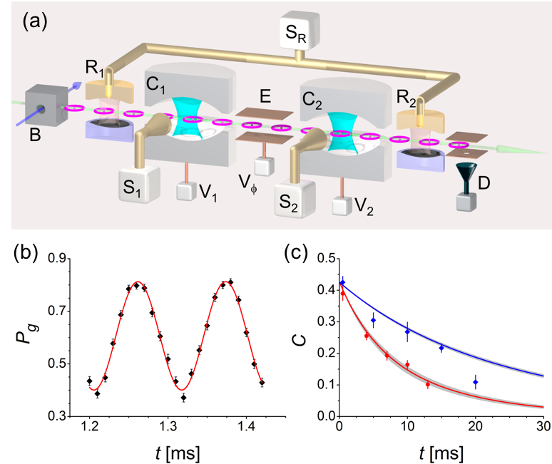
Figure 1: Preparation and detection of a two-cavity entangled state. (a) Scheme of the experimental setup with two microwave cavities (C₁, C₂) and circular Rydberg atoms, see text for details. (b) Quantum beat note between the two components of the non-local state $\left|\Psi(t)\right\rangle$ directly measured as $P_{g}(t)$. Error bars are statistical, the solid line is a fit with $f(x)=y_{0}-C/2\cos(\delta x\!+\!\varphi)$ ($0\leq C\leq 1$), leading to a $C_{0}=0.4$ contrast. (c) Time decay of $C$ revealing the decoherence of the two-cavity state. The experimental points are obtained by fitting the $P_{g}(t)$ oscillation signals around different $t$s for two cavity temperatures: 0.8 K (blue) and 1.5 K (red). The solid lines result from numerical predictions with $C_{0}$ as the only adjustable parameter. The shaded areas are numerical uncertainties resulting from the finite accuracy ($\pm 1$ ms) on the measured cavity lifetimes. The residual variance between the curves and the ensemble of points is compatible with the error bars, except for the longest time $t=20$ ms. The measured frequency drift of the two-cavity setup of several tens of Hz per hour (approximate acquisition time for the measurement with $t$ = 20 ms) results in a phase diffusion significantly reducing the oscillation contrast at this timescale.

We apply the reconstruction to the non-local entangled state $\left|\Psi\right\rangle=(\left|1,0\right\rangle+\left|0,1\right\rangle)/\sqrt{2}$, where one photon is coherently shared by C₁ and C₂. Its preparation is reminiscent of that of an entangled state of two modes of the same cavity Arno01 . An ‘entangling’ atom, A₁, is prepared in $\left|e\right\rangle$ in R₁ and tuned to resonance with the initially empty cavities. It experiences a $\pi/2$-Rabi rotation in C₁ and a state-swap with C₂ ($\pi$-Rabi rotation). Due to the $\delta=\omega_{c,2}-\omega_{c,1}=2\pi\times 8.9$ kHz detuning between C₁ and C₂, the state evolves as $\left|\Psi(t)\right\rangle=(\left|1,0\right\rangle+e^{i\delta t}\left|0,1\right\rangle)/\sqrt{2}$ within a proper phase reference and with the time origin $t=0$ set at the end of the $\pi$-Rabi pulse in C₂. Because of the probabilistic Poisson distribution of atoms in a sample and their non-ideal detection, the state $\left|\Psi\right\rangle$ is considered to be prepared if we detect only one atom in $\left|g\right\rangle$. The probability to have another non-detected atom during the entanglement preparation is about $3\%$.

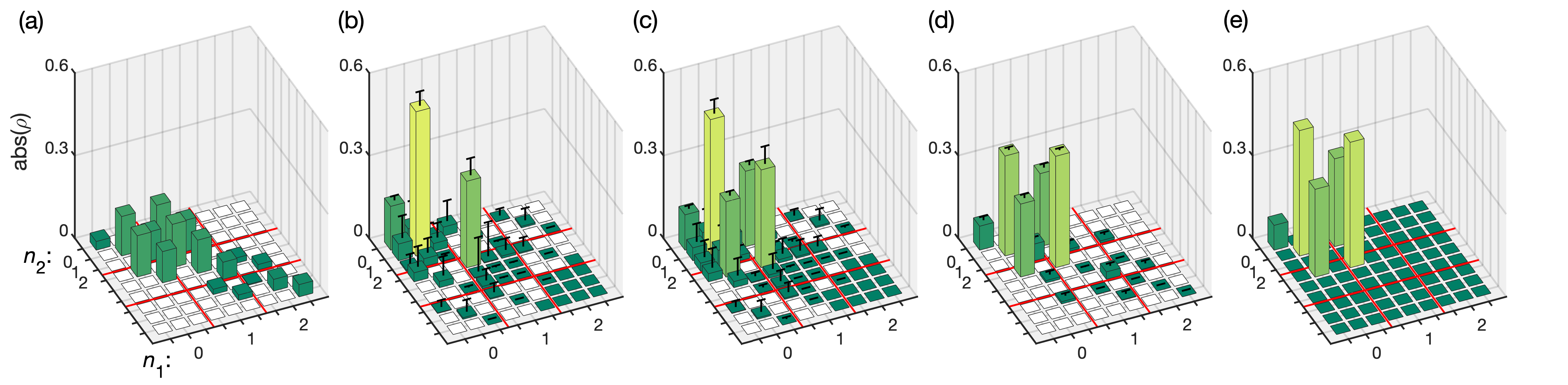
Figure 2: Absolute values of density matrix elements in a $3\!\times\!3$ two-cavity Hilbert space. Red guiding lines enclose areas with the same photon number in C₁; $n_{1}$ and $n_{2}$ are photon numbers in C₁ and C₂, respectively. (a) Reconstruction with single resonant atom measurements. (b) Reconstruction with QND parity measurement. (c) Reconstruction with both resonant and dispersive data of (a) and (b). (d) Reconstruction with sequences of several resonant measurements. Error bars $\sigma(\textrm{abs}(\rho_{\textrm{ML}}))$ in (a) are of the order of 0.5 and are not shown. Error bars smaller than $10^{-3}$ are not shown in plots (b)-(d). (e) Numerical prediction $\textrm{abs}(\rho_{\textrm{TH}})$ of the prepared state. The exact values of all reconstructed density matrices in the full $5\!\times\!5$ Hilbert space, together with their real and complex error bars, are given in SM .

For an elementary check of the state preparation, we use a probe atom, A₂, undoing the action of A₁ Arno01 . Initially in $\left|g\right\rangle$, A₂ performs a $\pi$-Rabi rotation in C₁ and a $\pi/2$-Rabi rotation in C₂. The probability $P_{g}$ for detecting A₂ in $\left|g\right\rangle$ at a delay time $t$ after A₁ is ideally $P_{g}=[1-\cos(\delta t+\varphi)]/2$ ($\varphi$ is a constant phase determined by the timing details). The oscillations of $P_{g}$ for short times $t$ around 1.3 ms are presented in Fig. 1(b). They have a finite contrast $C=C_{0}=0.4$, due to experimental imperfections. For larger times, $C$ decays with $t$, as shown in Fig. 1(c), due to photon loss at a rate depending on the cavities temperature, 1.5 K (0.8 K) for the red (blue) dots. The solid curves are numerical predictions with $C_{0}$ as the only adjustable parameter.

We now proceed to a ML reconstruction of the two-cavity state. We measure it by choosing between two types of the atom-cavity interaction: dispersive and resonant. We set resonant atoms, prepared in $\left|g\right\rangle$, to undergo the same temporal sequence as A₂. In addition to the unitary evolutions and relaxation in C₁ and C₂, the quantum map includes the detection imperfections as well as the small probability that a second, spurious atom present in the probe sample has escaped detection SM . Dispersive atoms are set to implement a quantum non-demolition (QND) measurement of the joint photon-number parity of the two cavities by setting $\delta_{ac}/2\pi\approx 60$ kHz Gleyzes07 . An atomic coherence, prepared by a $\pi/2$ pulse in R₁, is shifted by $\pi$ for each photon present in either cavity. This shift is probed by a $\pi/2$ pulse in R₂, the phase of which is set to maximize the probability for detecting the atom in $\left|g\right\rangle$ when both cavities are in the vacuum state. These dispersive probes do not change the photon numbers in C₁ and C₂. The measurements are intertwined with maps representing the free rotation of the two-cavity state at the frequency difference $\delta$ and the cavities relaxation. Optional field displacements are performed by S₁ and S₂ before the measurement. All quantum maps, including measurement imperfections, are given in SM .

We first analyse all data obtained with a single resonant probe that led to the results of Fig. 1(b) at 0.8 K. The sequence involves a free evolution and relaxation during time $t$ followed by a single resonant probe. The reconstruction is based on $3913$ realizations and performed in a tensor Hilbert space of dimension $5\!\times\!5$ (photon numbers $n$ from 0 to 4 in each cavity). The ML estimate, $\rho_{\textrm{ML}}$, is presented in Fig. 2(a). For the sake of visibility, we plot only the absolute values of the $\rho_{\textrm{ML}}$ elements for $n$ from 0 to 2 (the full $\rho_{\textrm{ML}}$ is shown in SM ).

Note that all two-cavity states of the form $\left|\Xi\right\rangle=(|n_{1},n_{2}\rangle+|n_{1}\!-\!1,n_{2}\!+\!1\rangle)/\sqrt{2}$ lead, for a resonant probe, to oscillations of $P_{g}(t)$ with the same frequency as those produced by $\left|\Psi(t)\right\rangle$, since their components also differ by only one photon and thus their energy difference is also $\hbar\delta$. The reconstructed $\rho_{\textrm{ML}}$ is thus a mixture of entangled states $\left|\Xi\right\rangle$. They appear with different weights, since the dependence of the Rabi oscillation frequency on the photon number brings ambiguous information on it. Due to this photon-number indetermination, the reconstruction error bars [not shown in Fig. 2(a)] are extremely large, of the order of 0.5 for all elements.

It is also important to note that the ML reconstruction may be blind to some elements of $\rho$. Writing $p_{r}(\rho)=\sum_{p,q}(\rho_{pq})^{*}E^{(r)}_{pq}$ in a generic basis $\{\left|p\right\rangle\}$, we see that $p_{r}(\rho)$ does not depend on $\rho_{pq}$ if $E^{(r)}_{pq}=0$ for specific $p$ and $q$ values. More generally, if no measurement contains information on $\rho_{pq}$ and thus $\sum_{r}|E^{(r)}_{pq}|=0$, the likelihood is independent of $\rho_{pq}$ and we get no more information on this specific matrix element than that provided by the positivity and unit trace of $\rho$. The blank elements in Fig. 2(a) correspond to those, on which the set of effect matrices provides no information.

An alternative measurement strategy providing better photon-number discrimination is based on QND joint parity measurements following adjustable coherent field injections (amplitudes $\alpha_{1}$ and $\alpha_{2}$) in the cavities Deleglise08 . This procedure amounts to a direct determination of the two-cavity Wigner function, $(\pi^{2}/4)W(\alpha_{1},\alpha_{2})$, at one point in the four-dimensional phase-space Schoelkopf16 . Here, for simplicity, we choose to inject in only one cavity at a time with 20 values of the injection amplitude ranging from 0 to 2.

Figure 2(b) shows the reconstructed state using 12200 realizations, each with 40 dispersive atom samples sent over a 4-ms time period. We now fully benefit from the efficiency of the method Six16 for a long sequence of successive measurements in a single realization. The reconstruction is sensitive to the photon number (diagonal elements) and to local, single-mode coherences between states $|n\rangle$ and $|n^{\prime}\rangle$ of the same cavity. Hence, the reconstructed state mainly includes $|1,0\rangle\langle 1,0|$ and $|0,1\rangle\langle 0,1|$. The significant contribution of $|0,0\rangle\langle 0,0|$ is due to atom and cavity relaxation during the state preparation. All other elements of $\rho_{\textrm{ML}}$ on which we get information are zero within their error bars. Note that this measurement does not provide any information on non-local coherences between the two cavities (blank elements in the figure).

The resonant and dispersive measurements provide complementary information on $\rho_{\textrm{ML}}$: the former is sensitive to non-local coherences, while the latter accurately reconstructs the photon-number probabilities. The reconstructed state consolidating the resonant and QND measurements data described above is shown in Fig. 2(c). Now, the dominant elements are the populations and coherences expected for $\left|\Psi\right\rangle$, showing that the data consolidation significantly improves the reconstruction.

As a reference to this reconstruction, Fig. 2(e) presents a numerical prediction, $\rho_{\textrm{TH}}$, of the prepared state. The model includes cavity and atomic relaxations, leading to the vacuum state population of 0.09. It also includes a reduction of the coherences by $30\%$ estimating the effect of stray electric fields inhomogeneity inside the atomic sample over the flight between C₁ and C₂. These stray fields perturb the phase of A₁ and, thus, the phase between the $\left|1,0\right\rangle$ and $\left|0,1\right\rangle$ components of $\rho_{\textrm{TH}}$. They contribute to the contrast reduction observed in Fig. 1(b).

The method does not require that the successive measurements commute , characteristic of the QND probes. We illustrate this unique feature by reconstructing the state with a long sequence of resonant probe samples. Each of them considerably changes the following measurement outcomes through its possible photon emission or absorption. We can nevertheless get useful information out of long sequences of non-ideally detected samples with a precise knowledge of the associated maps. The corresponding experiment involves $40$ resonant atomic samples separated by $0.2$ ms with, on average $0.15$ atoms per sample. The reconstruction result based on $18000$ realizations is presented in Fig. 2(d). The possibility of detecting more than one atom per realization indeed considerably improves the photon number determination with respect to Fig. 2(a). In addition, the long measurement duration improves the discrimination of small and large $n$’s, which have different lifetimes. Finally, using many samples significantly increases the information acquisition rate per realization.

We compute the fidelity $F(\rho,\sigma)=\left[\mathrm{Tr}\sqrt{\sqrt{\rho}\sigma\sqrt{\rho}}\right]^{2}$ between two different states $\rho$ and $\sigma$ in order to compare them. The fidelity of the reconstructed states of Fig. 2(a)-(d) with respect to the theoretical one [Fig. 2(e))] is 0.29, 0.85, 0.96 and 0.78, respectively. It is similar for the states (b) and (d), because the former is better in reproducing the expected populations in $\left|1,0\right\rangle$ and $\left|0,1\right\rangle$, while the former is better in the estimation of coherences. The large fidelity value for the state in (c) highlights the interest of consolidating many different measurements in the reconstruction, a key feature of our approach.

The method provides error bars for the density operator elements. In order to check that they faithfully describe the reconstruction precision, we apply the method to the estimation of a simple parameter and compare its predicted uncertainty to its experimental dispersion observed in many reconstructions. We have chosen to estimate the phase $\phi_{a}$ of the initial state $\left|\Psi_{\phi}\right\rangle\!=\!(\left|1,0\right\rangle+e^{i\phi_{a}}\left|0,1\right\rangle)/\sqrt{2}$, which is an essential characteristic of the prepared entangled state. This phase is tuned by applying an electric field across the electrodes E, sandwiched between C₁ and C₂ [Fig. 1(a)]. This field changes the phase of the coherence of A₁, which is finally imprinted into the phase of the two-cavity state. In the following, we prepare $\left|\Psi_{\phi}\right\rangle$ with $\phi_{a}\!=\!1.50\pm 0.03$ rad, independently calibrated with Ramsey spectroscopy.

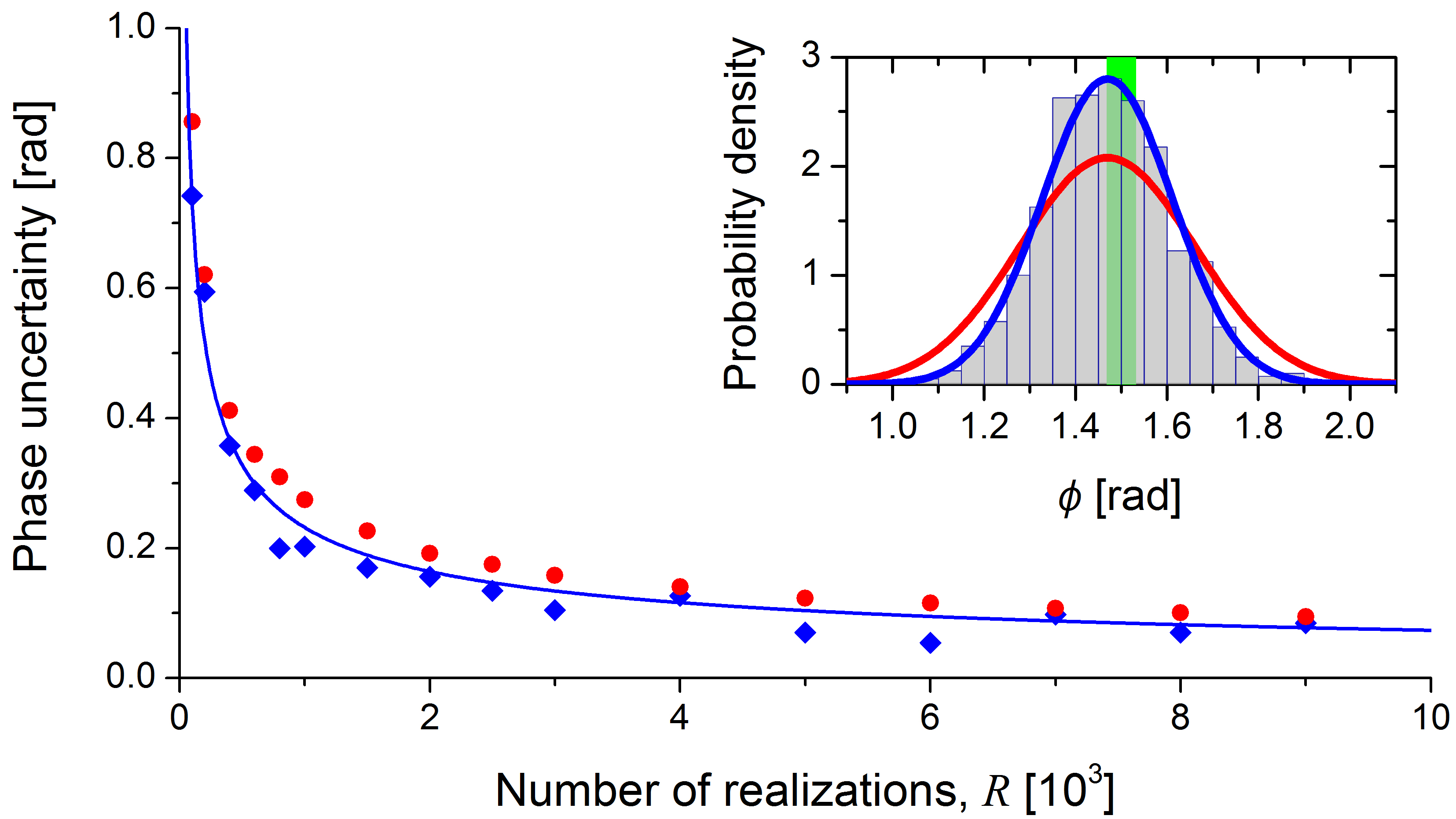
Figure 3: Statistical properties of the phase uncertainty. Blue diamonds: dispersion $\tilde{\sigma}_{\phi,R}$ of the reconstructed $\phi$ values versus the number of realizations $R$. Solid line: fit with a statistical dispersion function. Red circles: mean value of computed $\sigma(\phi)$. Note that having the limited set of all experimental realizations, we have fewer independent statistical sets of large size $R$. Therefore, there are fewer independent reconstructions and hence the larger statistical variance of reconstruction results for large $R$. Inset: distribution of $\phi$ from 800 reconstructions on samples with $R=2000$ realizations (histogram). Blue (red) line: Gaussian with width $\tilde{\sigma}_{\phi,R}$ ($\langle\sigma(\phi)\rangle_{R}$). Green band: independently measured confidence interval for $\phi_{a}$.

We implement a bootstrapping approach to estimate the reconstruction precision as a function of the sample size $R$ (number of realizations used for one reconstruction), see SM for more details. We calculate the standard deviation $\tilde{\sigma}_{\phi,R}$ of the reconstructed values of $\phi$ and the mean value $\langle\sigma(\phi)\rangle_{R}$ of the computed error bar $\sigma(\phi)$. Figure 3 shows $\tilde{\sigma}_{\phi,R}$ (blue diamonds) and $\langle\sigma(\phi)\rangle_{R}$ (red circles) versus $R$. Their values are nearly equal, exhibiting the accuracy of the error bar prediction. The solid line is a fit of $\tilde{\sigma}_{\phi,R}$ to a function $y(x)=A/\sqrt{x}$ confirming that the measured deviations have a purely statistical origin. The slight systematic excess of $\langle\sigma(\phi)\rangle_{R}$ with respect to $\tilde{\sigma}_{\phi,R}$ is potentially due to higher order correcting terms in the asymptotic expansion versus $R$ of Bayesian variances underlying $\langle\sigma(\phi)\rangle_{R}$ that corresponds only to the dominant term of order $1/\sqrt{R}$ SixPRPralyBook2017 . The inset in Fig. 3 shows the histogram of the individual $\phi$ values for $R=2000$. The green band gives the calibration of $\phi_{a}$ and its uncertainty. The blue (red) line is a Gaussian with width $\tilde{\sigma}_{\phi,R}$ ($\langle\sigma(\phi)\rangle_{R}$). These results confirm that the method provides realistic error bars on $\rho_{\textrm{ML}}$.

In summary, we have experimentally demonstrated on a two-cavity entangled state the pertinence and precision of the ML state reconstruction method proposed in Six16 . We have shown that it efficiently takes into account data provided by different measurement strategies as well as the system evolution during the measurement sequence. It integrates easily the description of measurement imperfections. We have shown that it provides realistic error bars for the reconstructed density matrix elements. The method is quite general and can be applied to nearly any quantum system and any measurement protocol, well beyond demonstrations in cavity or circuit QED Six16 . If the initial quantum state is known, the method can also be efficiently implemented for the parameter estimation Six16a . Finally, the analysis of the structure of the effect matrices provides a guide for designing adaptive reconstruction procedures Qi17 ; Pereira18 ; Struchalin18 by selecting optimal measurements.

- (1) M. Paris and J. Řeháček, Quantum State Estimation, Springer, Berlin, Heidelberg (2004)
- (2) Y. S. Teo, Introduction to Quantum-State Estimation, World Scientific, (2015)
- (3) A. Silberfarb, P. S. Jessen, and I. H. Deutsch, Quantum State Reconstruction via Continuous Measurement, Phys. Rev. Lett. 95, 030402 (2005).
- (4) D. Gross, Y. K. Liu, S. T. Flammia, S. Becker, and J. Eisert, Quantum State Tomography via Compressed Sensing, Phys. Rev. Lett. 105, 150401 (2010).
- (5) Y. S. Teo, H. Zhu, B.-G. Englert, J. Řeháček, and Z. Hradil, Quantum-State Reconstruction by Maximizing Likelihood and Entropy, Phys. Rev. Lett. 107, 020404 (2011).
- (6) B. Qi, Z. Hou, L. Li, D. Dong, G. Xiang, and G. Guo, Quantum state tomography via linear regression estimation, Sci. Rep. 3, 3496 (2013).
- (7) A. Kyrillidis, A. Kalev, D. Park, S. Bhojanapalli, C. Caramanis, and S. Sanghavi, Provable compressed sensing quantum state tomography via non-convex methods, npj Quantum Information 4, 36 (2018).
- (8) G. Torlai, G. Mazzola, J. Carrasquilla, M. Troyer, R. Melko, and G. Carleo, Neural-network quantum state tomography, Nature Physics 14, 447–450 (2018).
- (9) A. I. Lvovsky, H. Hansen, T. Aichele, O. Benson, J. Mlynek, and S. Schiller, Quantum State Reconstruction of the Single-Photon Fock State, Phys. Rev. Lett. 87, 050402 (2001).
- (10) H. Häffner, W. Hänsel, C. F. Roos, J. Benhelm, D. Chek-al-kar, M. Chwalla, T. Körber, U. D. Rapol, M. Riebe, P. O. Schmidt, C. Becher, O. Gühne, W. Dür, and R. Blatt, Scalable multiparticle entanglement of trapped ions, Nature 438, 643–646 (2005).
- (11) G. Zambra, A. Andreoni, M. Bondani, M. Gramegna, M. Genovese, G. Brida, A. Rossi, and M. G. A. Paris, Experimental Reconstruction of Photon Statistics without Photon Counting, Phys. Rev. Lett. 95, 063602 (2005).
- (12) W.-B. Gao, C.-Y. Lu, X.-C. Yao, P. Xu, O. Gühne, A. Goebel, Y.-A. Chen, C.-Z. Peng, Z.-B. Chen, and J.-W. Pan, Experimental demonstration of a hyper-entangled ten-qubit Schrödinger cat state, Nature Physics 6, 331-335 (2010).
- (13) D. Giovannini, J. Romero, J. Leach, A. Dudley, A. Forbes, and M. J. Padgett, Characterization of High-Dimensional Entangled Systems via Mutually Unbiased Measurements, Phys. Rev. Lett. 110, 143601 (2013).
- (14) N. Bent, H. Qassim, A. A. Tahir, D. Sych, G. Leuchs, L. L. Sánchez-Soto, E. Karimi, and R. W. Boyd, Experimental Realization of Quantum Tomography of Photonic Qudits via Symmetric Informationally Complete Positive Operator-Valued Measures, Phys. Rev. X 5, 041006 (2015).
- (15) C. Wang, Y. Y. Gao, P. Reinhold, R. W. Heeres, N. Ofek, K. Chou, C. Axline, M. Reagor, J. Blumoff, K. M. Sliwa, L. Frunzio, S. M. Girvin, L. Jiang, M. Mirrahimi, M. H. Devoret, and R. J. Schoelkopf, A Schrödinger cat living in two boxes, Science 352, 1087 (2016).
- (16) C. A. Riofrío, D. Gross, S. T. Flammia, T. Monz, D. Nigg, R. Blatt, J. Eisert, Experimental quantum compressed sensing for a seven-qubit system, Nature Communications 8, 15305 (2017).
- (17) A. Steffens, C. A. Riofrío, W. McCutcheon, I. Roth, B. A. Bell, A. McMillan, M. S. Tame, J. G. Rarity, and J. Eisert, Experimentally exploring compressed sensing quantum tomography, Quantum Sci. Technol. 2, 025005 (2017).
- (18) D. Ahn, Y.S. Teo, H. Jeong, F. Bouchard, F. Hufnagel, E. Karimi, D. Koutný, J. Řeháček, Z. Hradil, G. Leuchs, and L. L. Sánchez-Soto, Adaptive Compressive Tomography with No a priori Information, Phys. Rev. Lett. 122, 100404 (2019).
- (19) Z. Hradil, Quantum-state estimation, Phys. Rev. A 55, 1561 R (1997).
- (20) P. Six, Ph. Campagne-Ibarcq, I. Dotsenko, A. Sarlette, B. Huard, and P. Rouchon, Quantum state tomography with noninstantaneous measurements, imperfections, and decoherence, Phys. Rev. A 93, 012109 (2016).
- (21) S. Gammelmark, B. Julsgaard, and K. Mølmer, Past quantum states of a monitored system, Phys. Rev. Lett. 111, 160401 (2013).
- (22) M. Christandl and R. Renner, Reliable Quantum State Tomography, Phys. Rev. Lett. 109, 120403 (2012).
- (23) S. T. Flammia, D. Gross, Y. K. Liu, and J. Eisert, Quantum tomography via compressed sensing: Error bounds, sample complexity, and efficient estimators, New J. Phys. 14, 095022 (2012).
- (24) R. Blume-Kohout, Robust error bars for quantum tomography, arXiv:1202.5270.
- (25) P. Faist and R. Renner, Practical and Reliable Error Bars in Quantum Tomography, Phys. Rev. Lett. 117, 010404 (2016).
- (26) See Supplemental Material at […] for additional experimental and theoretical details, which includes Refs. HarocheBook ; Zhou12 ; SixPRPralyBook2017 .
- (27) S. Haroche and J.M. Raimond, Exploring the Quantum: atoms, cavities and photons, Oxford University Press, Oxford (2006).
- (28) Xingxing Zhou, Field locked to Fock state by quantum feedback with single photon corrections, PhD thesis, Université Pierre et Marie Curie - Paris VI (2012), https://tel.archives-ouvertes.fr/tel-00737657.
- (29) P. Six and P. Rouchon, Feedback Stabilization of Controlled Dynamical Systems, chapter Asymptotic expansions of Laplace integrals for quantum state tomography, Lecture Notes in Control and Information Sciences 473, pp. 307–327, Springer (2017).
- (30) T. Rybarczyk, B. Peaudecerf, M. Penasa, S. Gerlich, B. Julsgaard, K. Mølmer, S. Gleyzes, M. Brune, J.-M. Raimond, S. Haroche, and I. Dotsenko, Forward-backward analysis of the photon-number evolution in a cavity, Phys. Rev. A 91, 062116 (2015).
- (31) S. Gleyzes, S. Kuhr, C. Guerlin, J. Bernu, S. Deléglise, U. Busk Hoff, M. Brune, J.-M. Raimond, and S. Haroche, Quantum jumps of light recording the birth and death of a photon in a cavity, Nature (London) 446, 297 (2007).
- (32) C. Guerlin, J. Bernu, S. Deléglise, C. Sayrin, S. Gleyzes, S. Kuhr, M. Brune, J.-M. Raimond, and S. Haroche, Progressive field-state collapse and quantum non-demolition photon counting, Nature (London) 448, 889 (2007).
- (33) A. Rauschenbeutel, P. Bertet, S. Osnaghi, G. Nogues, M. Brune, J. M. Raimond, and S. Haroche, Controlled entanglement of two field modes in a cavity quantum electrodynamics experiment, Phys. Rev. A 64, 050301(R) (2001).
- (34) S. Deléglise, I. Dotsenko, C. Sayrin, J. Bernu, M. Brune, J.M. Raimond, and S. Haroche, Reconstruction of non-classical cavity field states with snapshots of their decoherence, Nature (London) 455, 510 (2008).
- (35) B. Peaudecerf, C. Sayrin, X. Zhou, T. Rybarczyk, S. Gleyzes, I. Dotsenko, J. M. Raimond, M. Brune, and S. Haroche, Quantum feedback experiments stabilizing Fock states of light in a cavity, Phys. Rev. A 87, 042320 (2013).
- (36) Pierre Six, Estimation d’état et de paramètres pour les systèmes quantiques ouverts, PhD thesis, PSL Research University (2016), https://tel.archives-ouvertes.fr/tel-01511698v1.
- (37) B. Qi, Z. Hou, Y. Wang, D. Dong, H.-S. Zhong, L. Li, G.-Y. Xiang, H. M. Wiseman, C.-F. Li, and G.-C. Guo, Adaptive quantum state tomography via linear regression estimation: Theory and two-qubit experiment, npj Quantum Information 3, 19 (2017).
- (38) L. Pereira, L. Zambrano, J. Cortés-Vega, S. Niklitschek, and A. Delgado, Adaptive quantum tomography in high dimensions, Phys. Rev. A 98, 012339 (2018).
- (39) G. I. Struchalin, E. V. Kovlakov, S. S. Straupe, and S. P. Kulik, Adaptive quantum tomography of high-dimensional bipartite systems, Phys. Rev. A 98, 032330 (2018).