Abstract

Conservation planning needs reliable information on spatial patterns of biodiversity. However, existing data sets are skewed: some habitats, taxa, and locations are under-represented. Here, we map geographic publication density at the sub-national scale of individual ’provinces’. We query the Web of Science catalogues SCI and SSCI for biodiversity-related publications including country and province names (for the period 1993-2016). We combine these data with other provincial-scale factors hypothesised to affect research (i.e. economic development, human presence, infrastructure and remoteness). We show that sites that appear to be understudied, compared with the biodiversity expected from their bioclimatic conditions, are likely to have been inaccessible to researchers for a diversity of reasons amongst which current or recent armed conflicts are notable. Finally, we create a priority list of provinces where geographic publication bias is of most concern, and discuss how our provincial-scale model can assist in adjusting for publication biases in conservation planning.

Introduction

National and international conservation policies rely on global biodiversity data sets. Repositories such as the IUCN Red List and the Global Biodiversity Information Facility (GBIF) synthesise existing data sets to support conservation planning. However, knowledge of the abundance and distribution of biodiversity remains patchy. Even the global number of species is unknown, and the spatial distribution of those species that have been described is often uncertain – knowledge deficits termed the “Linnaean” and “Wallacean” shortfalls, respectively ([Bri10]). Hence, there are continuing calls to improve biodiversity information ([JMG12]). Indeed, it would be informative to have ‘maps of ignorance’ that map and quantify present knowledge deficits ([Roc+11]). Concurrently, open access publishing policies and science communication strategies to redress the underrepresentation of less affluent regions need reform ([Wil+16]), such as better targeted research priorities.

The spatial patchiness of existing biodiversity data sets reflects historic and contemporary research efforts. Hence, these data sets incorporate biases, emphases and omissions (e.g. [Boa+10]). Research efforts have tended to focus on favoured taxa and habitats, such as vertebrates and forests ([FFL05]). Within taxonomic groups further biases exist. For example, research on felids is biased towards those with a large body size ([Bro09]) and [Bro+14] found that body size, range size and diet explain uneven patterns of research efforts across carnivores.

Uneven spatial patterns occur for a variety of reasons. Accessibility of is a strong influence on the likelihood of a location being researched. [RD03], for example, demonstrated that sampling locations of passerine birds in Sub Saharan Africa were clustered near roads, along rivers, and around urban areas. The practicalities faced by researchers striving to adapt to living and working conditions are amongst the components of accessibility. Socio-economic conditions (e.g. levels of affluence, infrastructure, language, security) privilege specific areas for research, and thus influence spatial sampling patterns ([MBE12, AS13, Mey+16]).

For example, [Fis+11] showed that research efforts on coral reefs were positively correlated with an area’s per capita gross domestic product. Research effort is also known to cluster around areas that have previously been deemed of interest. This might be considered a consequence of their already documented biodiversity and consequently known threats to the biodiversity of these areas, but may also be due to the practical and infrastructural benefits provided by biological field stations and established monitoring sites (see [Tyd+16]). Thus, [MBE12] demonstrated that protected areas are over-represented, as are sites in temperate deciduous woodlands and wealthy countries. Whatever the causes, these biases can lead to a self-reinforcing cycle whereby ‘funding begets biodiversity’ ([Ahr+11]).

The geographic sampling biases in biodiversity research have implications for macro-ecological modelling ([YMK13]), conservation prioritisation [DMN11], and governance audits like those of the Intergovernmental Science-Policy Platform on Biodiversity and Ecosystem Services (IPBES). While modellers have developed methods to correct for sampling biases in species range modelling ([Kra+13, Eng+15]) and in applying systematic conservation planning tools ([Ron+06]), such remedies cannot always address the persistent undersampling of biodiversity ([Wil+16]). For example, ([Gre+06]) demonstrated little spatial congruence between the occurrence of threatened bird and mammal species (or across these taxa) at the spatial scales relevant for conservation planning. In addition, re-directing effort from well-sampled towards under-sampled locations may improve the efficiency of conservation actions ([Ara+11]).

[SL09] demonstrated that, under some plausible assumptions, if the aim of a study is to describe the spatial distribution of species richness in a given area, then surveying under-sampled locations is more effective than surveying areas known to be of high species richness. [DMN11] used a simulation study to find out that focussing on poorly surveyed areas maximises the benefits of surveys for conservation planning.

We developed a global, provincial-scale map of biodiversity publication density to identify areas where low accessibility is associated with research deficits. We define ‘provinces’ as sub-national administrative units, as recognised in the Global Administrative Areas database ([GAD]), covering differently named areas (e.g., provinces, departments, counties) of various size. For each province, we mapped the number of biodiversity research publications by area using the Web of Science catalogues SCI and SSCI. This map can be considered a surrogate for sampling effort, as demonstrated by [Lob08]. We modelled the associations between factors affecting accessibility (i.e., remoteness, infrastructure, and development) and publication density, identifying provinces where the shortfall in publications is linked to accessibility, but where human impact on biodiversity is also very likely. We suggest that such a ‘map of ignorance’ can facilitate a prioritisation of future biodiversity research that adjusts for current bias.

Methods

For each province we queried the Web of Science (WoS) catalogues SCI and SSCI for publications labelled in the “Biodiversity & Conservation” category (covering publications appearing in any journal listed under that category; not to be confused with the journal of the same name) that included the country name (in multiple languages and writing styles) as well as the province name. We limited our search to the period 1993 to 2016 – starting with the United Nations Earth Summit conference in Rio de Janeiro, to capture a period of sustained global research in biodiversity. Many more biodiversity publications were identifiable to country level (n= 1,229,636) than to province level (n = 54,144). As some provinces had no results for the biodiversity and conservation WoS category, we inferred values for the number of publications based on the ratio of biodiversity research to overall research within a country. Assuming that this proportion was constant for a country we multiplied the province’s overall total number of publications by this proportion and adjusted the result by province area (n= 44,858 publications on province level, see Supplementary Information (SI) for details). We refer to this hereafter as ‘inferred publication density’, with publications per km² as the unit.

The queries were performed using the R-package rwos ([Bar19]) and the Web of Science Lite API ([Reu12]); country and province name were taken from the GADM data set ([GAD]) and the R-package countrycode ([Are19]) and results were filtered in the different Web of Science domains (all = no constraint, cons = biodiversity and conservation as single category). The map of inferred biodiversity publication density was produced in R-language 3.1 with the script in [Hic17a].

We hypothesised that the publication density in a province would be affected by the degree of accessibility of that province for researchers. Given that there were numerous potential drivers affecting both accessibility and biodiversity, we used an ordination technique to reduce the data to a small set of orthogonal axes summarising the input variables. We conducted a Principal Components Analysis (PCA) using the prcomp function in R. We used two proxies of ecological conditions: mean precipitation and temperature data derived from Worldclim ([FH17]); two measures of human presence: one based on the NASA night-time light data set corrected for gas flares ([NGD13]) and the other derived from weekly fire clusters of the NASA VIIRs data set ([NAS]). Within the data on fire clusters we corrected for large bushfires by spatially clustering reported fire points by week (see SI; weekly fire clusters may be a better indicator than simple fire point counts, as these remove the effects of large bush fires that can ignite naturally or result from a one-time human action). These fire indices complement those quantifying human footprint insofar as the latter fail to capture the impact of nomadic agro-pastoral communities. We also developed a remoteness index based on mean travel time to major cities, capitals, airports and seaports ([Nel08, Gir19]) and a world road area index (derived from [Ibi+16]). We used mean life expectancy at birth (from 1966 to 2016) as a measure of human development as well as an index of the relative living conditions in a province ([Gro]). We cut all geo-spatial data to the extent of the province shape, and calculated mean values (for raster data), as well as the size (in m²) and counts for all vector data sets. These data are stored on file per GADM province record (see SI 5 for further details). We had to remove 53 of 204 countries, and 184 of 3,417 provinces prior to the PCA, due to missing data. In most cases, the missing data related to life expectancy and applied to small island groups. These are often not listed separately in the relevant World Bank data sets. We log-transformed the variables with large variance and high skew (i.e., publication density, road area, fire clusters, and remoteness), and corrected for province area. We plotted location of provinces as a function of PCA 1 and PCA 2 scores using the ggfortify R-package ([THL16]).

We fitted a linear model for the subset of provinces where the number of publications was known, and used inferred publication density as the response and actual conservation publications as predictor. We also fitted a model for the same subset with the remoteness index as response, and night light intensity, road and province area measures as predictor. A third model used the fire clusters as response and the night lights and WDPA Category I and II protected areas as predictors. Finally, we ran a linear mixed effects model (LMER) with inferred publication density as the response, and the above variables as predictors, correcting for country as a random effect, and also incorporating protected areas and IUCN terrestrial mammal ranges ([IUC]) to assess which predictors best explain observed patterns in biodiversity publication density (taking into account any pattern of collinearity among them). Full details of all provinces are available online and in the Appendix (see Table 4) and online ([Hic]).

We identified priority provinces, where remoteness was most strongly linked to publication density and where climate (and latitude) indicate that biodiversity is likely to be high. We did so by summing the absolute axis scores of the synthetic component PC1, and the synthetic component PC2 for those provinces in the quadrant most characterised by remoteness and high number of fire clusters.

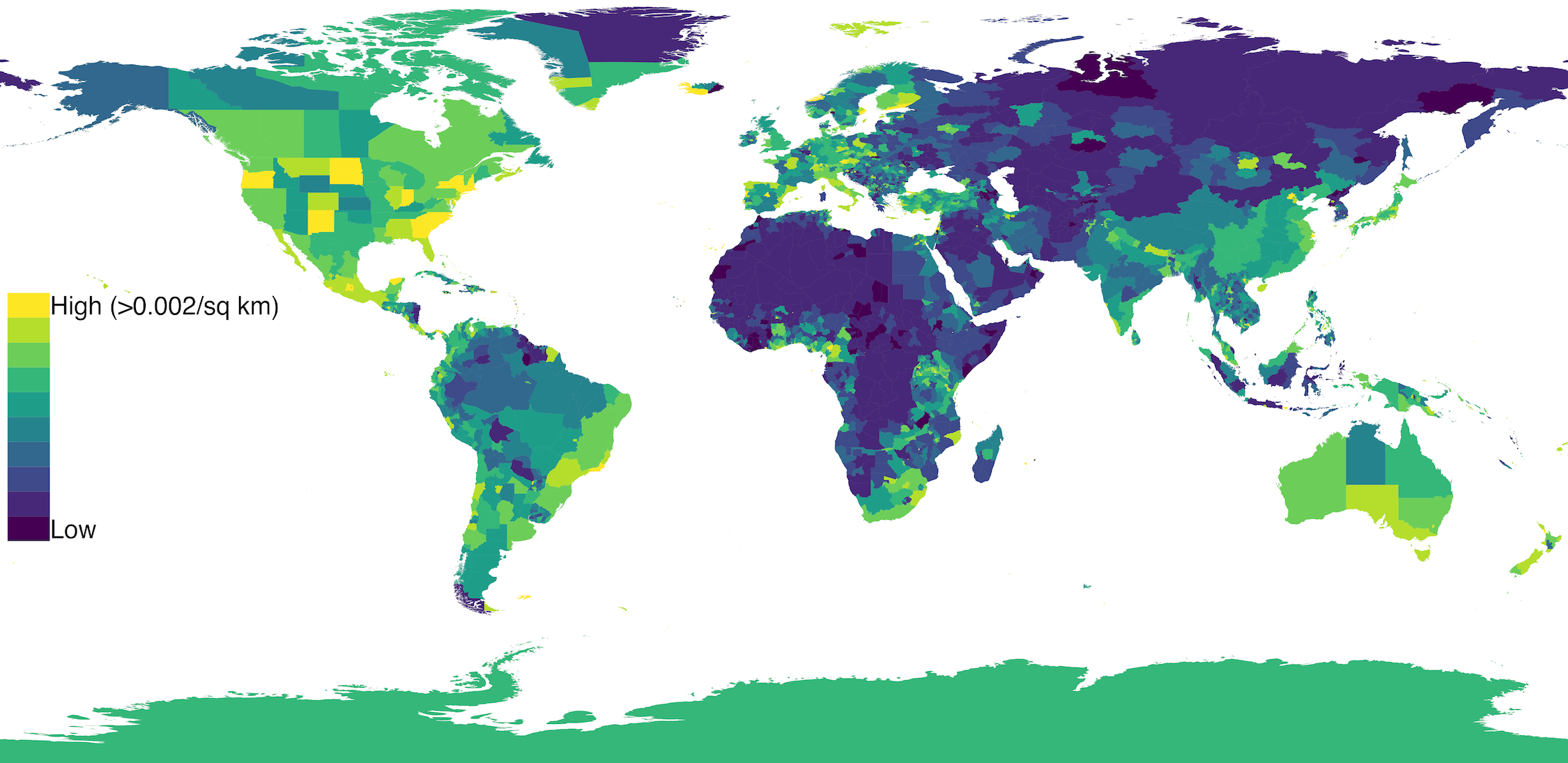
Figure 1: Map of publication density. Map of density of publications of the biodiversity and conservation category in the Web of Science SCI and SSCI catalogues that mention country and province name (recording period: 1993 to 2016), adjusted for the geographic size of the provinces (km²). The data for this map is available at [Hic17]; An interactive version of this map is available at bit.ly/publication_density_map

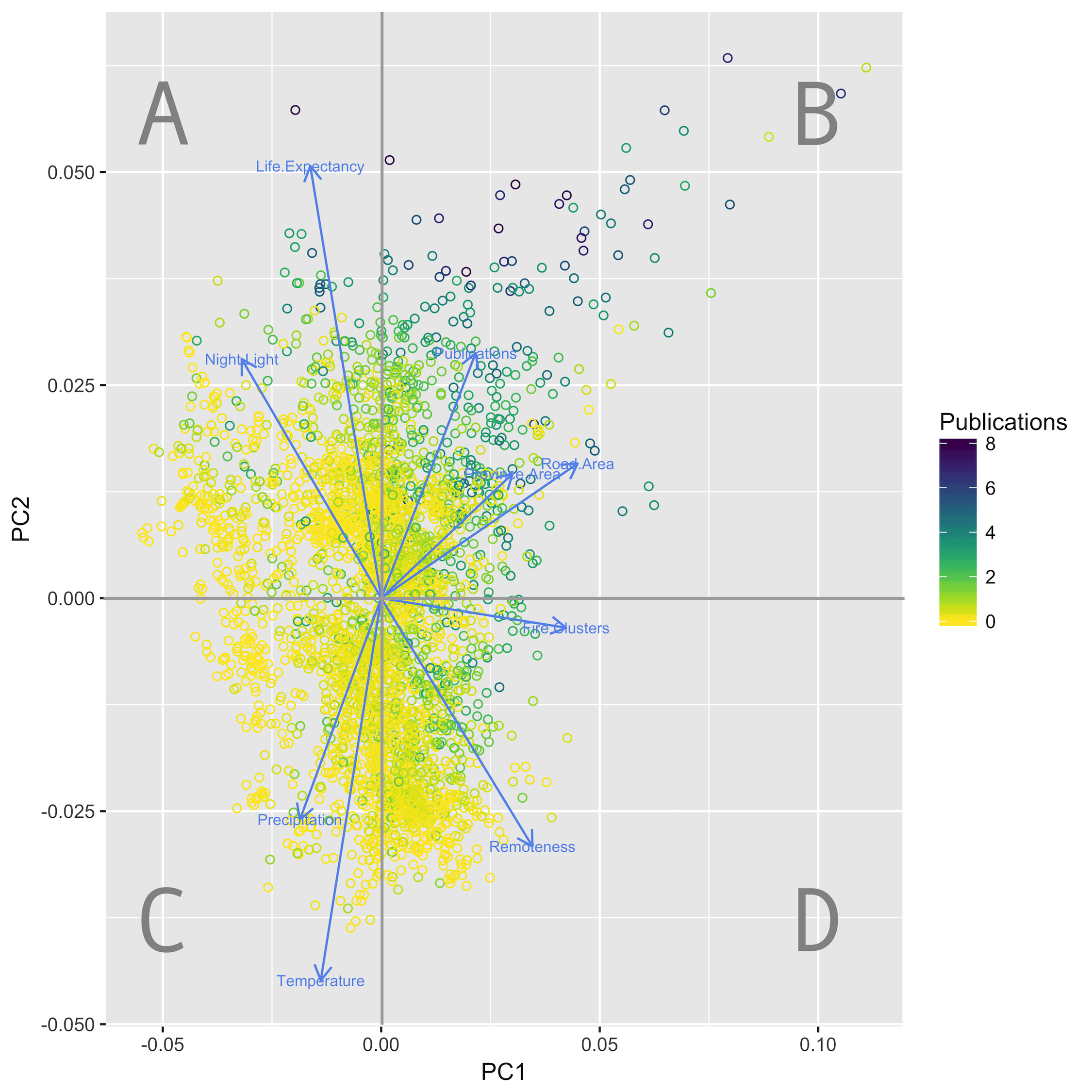
Figure 2: Principal Component Analysis plot PC1 PC2. Dots represent provinces, and color indicates log transformed biodiversity and conservation related publication density (data available at [Hic17c]). The tropical provinces (high temperature and precipitation) that are less affluent (life expectancy) show low economic activity (nightlight), are remote (remoteness), and exhibit high human presence (fire clusters). In general, these provinces appear less studied – even though they are often located adjacent to known biodiversity hotspots.

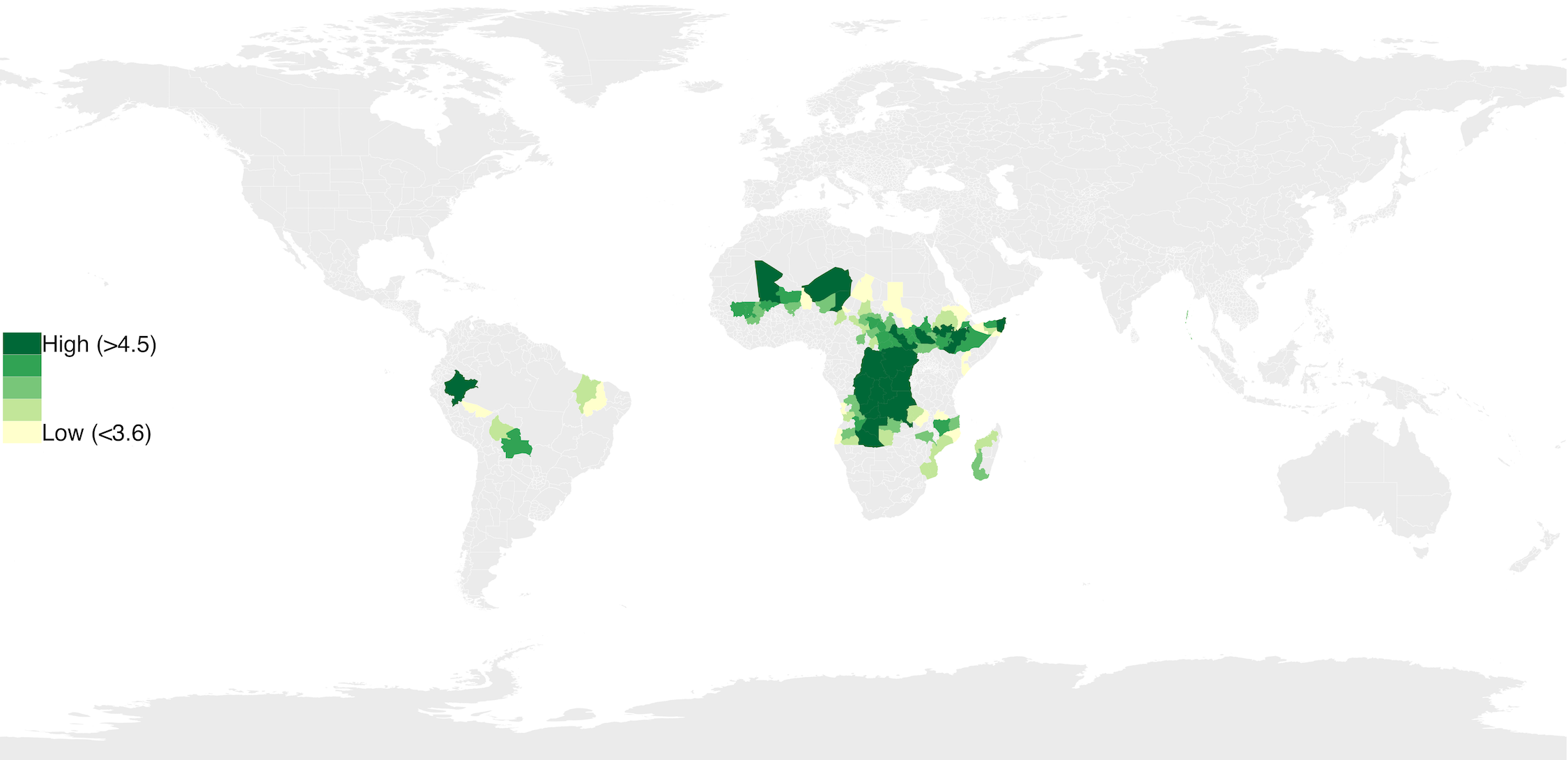
Figure 3: 100 Priority Provinces. The location of 100 priority provinces where the accessibility bias in geographic reporting bias is most apparent. Provinces of Quadrant C in the PCA (see Fig. 2) are ranked by their combined coordinate score (PC1 positively and PC2 negatively) and indicated by color (data at [Hic17c]

Table 1: Results of linear mixed model with the number of publications in the Web of Science biodiversity and conservation category as response, and predictors used in glmm model.

Response	Predictor	Level	Estimate	SE	p-value
Publications	Number.ProtectedAreas	Province	7.53E-02	1.31E-02	8.65E-09
	Number.TerrestrialMammals	Province	8.14E-02	2.21E-02	2.37E-04
	ProtectedArea.Area.Cat.IabII	Province	7.42E-02	1.16E-02	1.91E-10
	Night.Light	Province	2.10E-01	1.48E-02	2.00E-16
	Life.Expectancy	Country	1.21E-01	4.94E-02	1.53E-02
	log(Road.Area)	Province	2.79E-01	2.34E-02	2.00E-16

Results of linear mixed model with the number of publications in the Web of Science biodiversity and conservation category as response, and predictors used in glmm model, mainly derived from spatial data sets (3428 observations). Life Expectancy is available only at the country level (n=204), hence country was used as grouping variable.

Results

The highest density of publications in the biodiversity and conservation WoS category were observed in more affluent countries and those with known biodiversity hotspots (Fig. 1). As expected from the latitudinal biodiversity gradient theory, high latitude areas were associated with lower publication density. At the same time, publication density was low for some areas close to the equator, such as Central Africa, too.

There was a positive and significant correlation between the number of biodiversity and conservation publications at province level and the inferred number of publications (R² = 98.4%), based on the assumption that the number is proportional to the size of the province; the inferred number predicted almost all the variation in the real number.

The remoteness index increased with the area of a province, and decreased with night light level and road density (total R² = 45.0%, model details in SI). The fire cluster index decreased with increasing electrified areas (night light intensity) and with increasing protected areas (total R² = 61.0%).

The number of inferred publications of a province correlated most strongly with the country’s inhabitants’ life expectancy at birth, night light intensity, and log-transformed road area (see Table 1). The number of biodiversity and conservation publications associated with a province increased with the indices of human development scores and road area (see Table 1). There was also a positive correlation between publication density and the number of protected areas in the respective province (see Table 1), as well as with the number of terrestrial mammal species present in a province according to IUCN distribution range maps.

The PCA (Fig. 2) demonstrates correlations between research deficits (low numbers of publications) and accessibility (i.e. lower than mean values of life expectancy, night light, road area, and remoteness). The first two components together explained 54.1% of the variance in the input variables (see SI). Visually, four distinct groups of provinces could be defined, corresponding to the quadrants of the PCA (A – D; see Fig. 2). Quadrant A encompassed provinces characterised by high levels of human development (i.e. high life expectancy) and high economic activity (in terms of night light). In addition, these provinces exhibited a high number of biodiversity publications as well as low temperature and low rainfall, compared to provinces in Quadrants C and D. Quadrant B included provinces characterised by high number of biodiversity publications, high density of roads and large area; again with relatively low temperature compared to provinces Quadrants C and D. Quadrant C included primarily tropical provinces, characterised by high temperature and precipitation, with low number of biodiversity publications (relative to Quadrants A and B), and lower degree of remoteness than those on Quadrants B and D. Accessibility issues may be of less relative importance in provinces located in Quadrant C. Finally, Quadrant D contains provinces that exhibit a low number of biodiversity publications, but high levels of remoteness (long travel times to major cities, capitals, seaports, and airports) and distinct human presence. At the same time, these provinces are located in less affluent regions, characterised more by fire clusters rather than by road area and night light.

Fig.  3 shows the scores of the ‘top 100’ priority provinces (largely within 15 degrees latitude to the equator) for which the factors in Quadrant D (Fig. 2) where the accessibility bias in geographic biodiversity reporting is likely to be of most influential (full list of “priority provinces”: 8).

Discussion

In this paper, we identified provinces with marked differences between the actual density of publications concerning biodiversity and conservation and the expected density of publications based on bioclimatic conditions and the latitudinal diversity gradient ( [Gas00, Hil04, Man+14]). Differences between actual and expected publication density are most likely to be related to the degree of accessibility of provinces. By integrating a large array of available data sets, the methodology presented here may provide a useful tool in optimizing future biodiversity monitoring and research efforts, regionally and globally.

Here we discuss the choice of complementary geospatial indicators. Based on recent case studies from Central Africa we moreover exemplify what a blurred view on the state of biodiversity in some provinces can imply. In addition we illustrate how an improved understanding of situation in 100 priority regions can make the management of well-known biodiversity hotspots more resilient.

Conventional indicators of the human footprint, such as the occurrence of roads, villages, and an index of night light, may underestimate the actual human impact in some provinces. For example, using fire clusters as a complementary indicator will allow assessing the effects of pastoralism and land clearance for farming, which have remained invisible for long periods. This indicator reveals an additional category of under-studied provinces located in Quadrant D (Fig. 2), which are of particular concern for current and future conservation efforts. These provinces are expected to exhibit high biodiversity. However, road infrastructure is poor and security may be limited, therefore knowledge about actual biodiversity status may be limited too (see [RD03]).

Most biological field stations are located in or close to protected areas. Concurrently, many of these areas are protected due to their high biodiversity, which again creates a positive accessibility bias towards these areas ([Tyd+16]). In addition, funding opportunities are most likely higher for these areas, compared to unprotected ’biodiversity hotspots’ ([Ahr+11]). Similarly, the positive correlation between publication density and terrestrial mammals’ distribution ranges can be interpreted as reflecting appropriate targeting of the areas of most need. Furthermore, species distribution range maps are frequently the outcome of biased reporting efforts. For example, range contraction estimates of the African lion in Central Africa are based on only very recent field observations (H. Bauer, personal communication, August 30, 2017; [BCS15]).

The 100 priority provinces exhibiting distinct gaps in biodiversity-related research, primarily due to low accessibility, share common attributes (see Fig. 3). These provinces are not necessarily very rich in biodiversity; however, they are located in remote areas, exhibit low human development index scores, and contain poor infrastructure. Most priority provinces are located in Central Africa, central Western Africa, Bolivia and the Amazonian regions (Peru and lowland areas of NE Brazil), as well as in the Andaman and Nicobar islands (India; see Fig.  3).

The inclusion of fire clusters in the model reflects the intensity of human impact in those provinces where standard indicators (i.e., night light, road area) would not detect human impacts. Therefore, our list of priority provinces considers ‘potential threat’; in addition to actual research deficits. Indeed, we did not highlight provinces that have low publication density and low human presence (as measured by fire clusters) as biodiversity in these areas is presumably under a lower level of threat - although these provinces may exhibit important knowledge deficits too. Provinces with these characteristics are located in the Amazonas Region in Brazil, the Caribbean Coast of Nicaragua, Sipaliwini in Suriname, most of Gabon, and in South Kalimantan and Sumatera Selatan (Indonesia).

Our results demonstrate that the patterns of under-reporting at a provincial scale are by no means homogenous. If poorly-researched provinces were randomly distributed, then adjacent provinces could be deemed ‘representative’. However, many under-reported provinces, with accessibility issues, have faced serious geopolitical challenges in recent decades. Many of these areas have experienced violent conflicts including inter-state wars, civil wars, rebel insurgencies, piracy, drug wars, and other forms of lawlessness. Moreover, poor security impairs funding and hinders field research ([Sut+12]). For example, violent conflicts lead to the destruction of habitats, bushmeat poaching by combatants and displaced communities, poaching for the illegal wildlife trade, persistent social disruption and a lack of conservation capacity ([Gay+16, Nac+14, CGM17, DP18]). Hence, knowledge gaps further deepen threats to wildlife populations, which therefore often go unnoticed.

For example, 7 out of 17 provinces in the Central African Republic (CAR) are part of our priority list of 100 under-reported areas with accessibility issues. These include the Mbomou and Haute-Kotto provinces, where the Chinko nature reserve was established in 2013 (R. Hickisch, personal communication, January 12, 2018). This reserve covers 19,840 km² and is among the largest managed protected areas in the entire region. In this area, the accessibility challenge is considered a consequence of continuing violence and geographic remoteness, which constrains logistics and increases costs. The resource-rich provinces of CAR and adjacent countries have experienced cycles of conflict and civil war for much of the past three decades ([Col08]). Many rebel groups, including the Lord’s Resistance Army, have sought refuge in remote, ungoverned, and most likely wildlife-rich provinces ([Ond+17]). Hence, it remains a major challenge to operate any kind of business in this region, in particular conservation activities, which require large numbers of staff. In addition, universities may be reluctant to provide insurance for their staff to operate in regions for which travel warnings have been issued.

Consequently, a lack of knowledge may constrain long-lasting conservation planning. For example, the Chinko basin formerly contained an elephant population numbering thousands of individuals (Douglas-Hamilton, 1987). Subsequently the population has crashed to a few hundred, or even fewer, individuals ([HA13]), due to ivory poaching. The population decline went largely unrecorded. Since the millennium, major poaching-induced population declines have occurred in Garamba National Park in the Democratic Republic of Congo ([Can15]) and in Zakouma National Park in Chad ([Fay07]) too. Again, these declines occurred in under-reported, accessibility-challenged provinces included on our priority list. Knowledge deficits and failures to learn from under-reported events are not limited to elephant populations. The latest IUCN report on African freshwaters life ([BAD11]) records a freshwater species richness of the Chinko drainage system similar to large parts of the Sahara desert (i.e., presumably 0). Since 2014, however, the Chinko river has been known among fly-fishing enthusiast as a favoured habitat for Goliath Tiger fish (F. Botha, personal communication, Apr 10, 2014). Hydrocynus goliath is a very large predatory fish (max. length: 1.5; max. body mass: 50 kg), documented in the Congo River basin to which the Chinko river is a tributary via the Oubangui river. A similar pattern applies to the Pousargues’s mongoose Dologale dybowskii: Large parts of its known distribution range overlap with territory of the Lord Resistance Army. The description of this species is thus based only on a few recent observations and museum specimen. It has a data deficient status in the IUCN redlist ([Aeb+15]).

However, knowledge gaps are not constrained to the status and trend of single species. For example, significant changes in the practices of pastoral communities are occurring in many less accessible provinces in central Africa (The Economist, 2017, November 9); and these changes have been largely unrecognised by conservation research. Social changes, the legacy of violence, and economic factors are leading to larger domestic stock herd-sizes, and climatic factors combined with increases in vaccine availability are allowing movement of these herds into areas formerly unsuitable for grazing (e.g., tse-tse fly habitats). Changing practices of transhumance – larger herd sizes, widespread availability of automatic weapons, and highly potent poisons threaten wildlife in multiple ways: from bushmeat hunting to the eradication of top predators ([Bou+10, BCS15]). Whilst the movements of these large herds can be monitored through remote-sensing methods – for example as fire cluster data as used herein – the subsequent impacts on wildlife (especially terrestrial mammals and birds) are more difficult to assess remotely, particularly if dense vegetation appears largely intact. The lack of adequate data on the response of wildlife to these changes is important in its own right, but it also represents a missed opportunity to understand and address these issues before they spread to nearby areas – as it is occurring with respect to large-herd shifting pastoralism. Interestingly, although the priority provinces we identify largely fall outside of ‘biodiversity hotspots’, as defined by [Mye+00], they are almost all adjacent or connected to areas of high conservation concern.

Addressing the systematic under-reporting of biodiversity in less accessible provinces is by no means a simple issue. Indeed, we do not propose that scientists should ignore the risks involved in working in remote provinces – but we do highlight the consequences of their current aversion to these risks. However, we do suggest that greater attention should be afforded to the accessibility bias that we have demonstrated in existing data sets, and to develop steps to narrow these gaps. We consider our provincial-scale model a first step for action, and we have made all the data open accessible ( [Hic17a, Hic17b]) to assist in this endeavour.

Supporting Information

Data sources

The data used includes:

• The Global Administrative Areas ‘GADM’ dataset mapping global political boundaries ([GAD]);

• The NASA night-time light data ([NGD13]) as a proxy for spatial economic activity;

• The weekly fire clusters of the NASA VIIRs data set ([NAS]) as a proxy for human presence (and labelled as a ‘human presence index’)

• Mean precipitation and temperature data from Worldclim ([FH17]) fas a proxy for possible biodiversity;

• A remoteness index constructed using data on: (1) mean travel time to major cities ([Nel08]), and (2) Mapbox Directions ([Map]) travel times from polygonal centre points (centroids) to capitals ([Gir19, Rud18]), airports ([Our]), and seaports ([Age]). The remoteness index is a measure of the cost and complexity of logistics related to conservation research and action.

• A dataset on world road area ([Ibi+16]) as a proxy for permanent infrastructure.

• The mean life expectancy at birth (from 1960 to 2010) as a proxy for the level of afflluence ([Gro]).

• The conservation knowledge data set that we created from the inferred number of Web of Science publications in the Biodiversity and Conservation category of SCI and SSCI catalogues (from 1993 to 2016; [Reu12]).

• The estimated number of terrestrial mammal species present per country, as well as their range ([IUC]) and the WDPA dataset on protected areas ([WDP]) as control indicator for present biodiversity.

Data Preparation

The datasets listed above were downloaded from the Internet, and converted into Feature Collections according to the OGC GeoPackage Encoding Standard ([OGC]). Using the GDAL command line tool ogr2ogr ([Fou19]) polygonal datasets were simplified by removing extraneous bends while preserving essential shape with a threshold of 0.0002 degrees. As not all polygonal data had been available in valid form (according to the OGC standard) the st_makevalid function of the Postgis ([Str16]) library liblwgeom was used to solve geometry problems.

We initially tried the Natural Earth airport dataset ([Nat17]), however, because of this data set being very limited, we opted instead to use the filtered records for the large_airport and medium_airport records from the ourairports dataset ([Our]) instead.

The world capital city data set was derived using the hrbrmstr R Openstreet Map Overpass query library ([Rud18]) query for administrative centre using the below R code.

library(overpass)
osmcsv <- ’
relation["admin_level"="2"]["type"="boundary"]["boundary"="administrative"];
node(r:"admin_centre");
out meta;’
opq <- overpass_query(osmcsv)
head(opq)
write.csv(opq, file = "capital_cities.csv")

Data Processing

We extracted spatial data from the above mentioned sets by the level 1 administrative boundary polygons from the GADM v2.8 dataset (also referred to as ‘province’; [GAD])  and saved them to file using country ISO code and province id (all processed data is available online:  [Hic17, Hic, Hic17c]).  For countries where only level 0 data was available, we used these instead.

All spatial datasets have been aggregated by averaging (for raster data), summarising areal extent (for polygons; in sq m) and/or counting (for points and polygons) and joining non spatial data (e.g. Life expectancy) using the R script available ([Hic17b]).

The summary of all province level data, including transformed (log, division by area) are available ([Hic]); all prepared input data is available here [Hic17c]

Table 2 shows the correlation matrix of all model input variables prepared in the data processing.

Table 2: Correlation matrix of model input variables

fire_clusters	1
log_province_road_area_2	0.78**	1
province_pa_area	0.24**	0.22**	1
log_province_area_m2	0.82**	0.92**	0.27**	1
province_pa_area_Iab_II	0.19**	0.20**	0.74**	0.25**	1
province_nightlight	-0.35**	-0.38**	-0.10**	-0.51**	-0.09**	1
Publications	0.26**	0.35**	0.22**	0.28**	0.24**	0.05**	1
province_pa_area_count	0.19**	0.31**	0.16**	0.21**	0.20**	0.01	0.39**	1
province_area_species_count	0.57**	0.36**	0.23**	0.50**	0.16**	-0.31**	0.11**	-0.01	1
province_pa_area_Iab_II_count	0.13**	0.18**	0.28**	0.15**	0.57**	-0.05**	0.28**	0.32**	0.06**	1
country_SP.DYN.LE00.IN	-0.25**	-0.05**	0.00	-0.26**	0.04*	0.37**	0.18**	0.18**	-0.46**	0.12**	1
province_num_conflict	0.02	0.05**	-0.01	0.06**	-0.01	-0.04*	-0.02	-0.02	0.02	-0.01	-0.14**	1

Indicator of Road Area

Road Area is calculated by subtracting summarised roadless area (Ibisch et al. 2016) from the GADM administrative polygon (GADM.org 2017) in order to represent the known presence of infrastructure (and solve issues for Greenland and Antarctica, which have no roads).

Caveats: not all roads are documented; more roads are documented in better connected/developed areas

Indicator of Human Presence

We decided not to use the Global Human Footprint dataset as a proxy for human presence. It represents human presence as complex composite variable of data on roads, villages, cropland, and other land asset-related variables (Sanderson et al. 2002). However, global roadmaps (and road less areas, such as (Ibisch et al. 2016)), and maps of villages (Socioeconomic Data and Applications Center 2017), and even river data sets (arcgis.com 2017) are much better mapped in provinces of larger wealth (Ibisch and Selva 2017). Therefore, a particular drawback is that it largely underestimates the impact of relatively small groups of people roaming vast areas, such as transhumant herdsmen in the Sahel.

Instead, we opted to use data on fire as a measure of human presence (see Fig 4). The high resolution NASA VIIRS data set on global daily fire points is available to the public from January 2016 onwards. To correct for large bushfires, eventually resulting in many such non-independent fire points along a front, we spatially cluster these points by cutting a weekly dendrogram of geolocations of these fires at the first level (using the R functions cutree and hclust), and subsample randomly if a province has more than 20,000 fire points in a single week. The resulting count of fire clusters provides a complementary indicator of human presence. We tested how well our indices of road coverage, protected areas and night light predicted the clusters. Together, these accounted for 61% of variation among princes in the frequency of fire clusters. Below the model output.

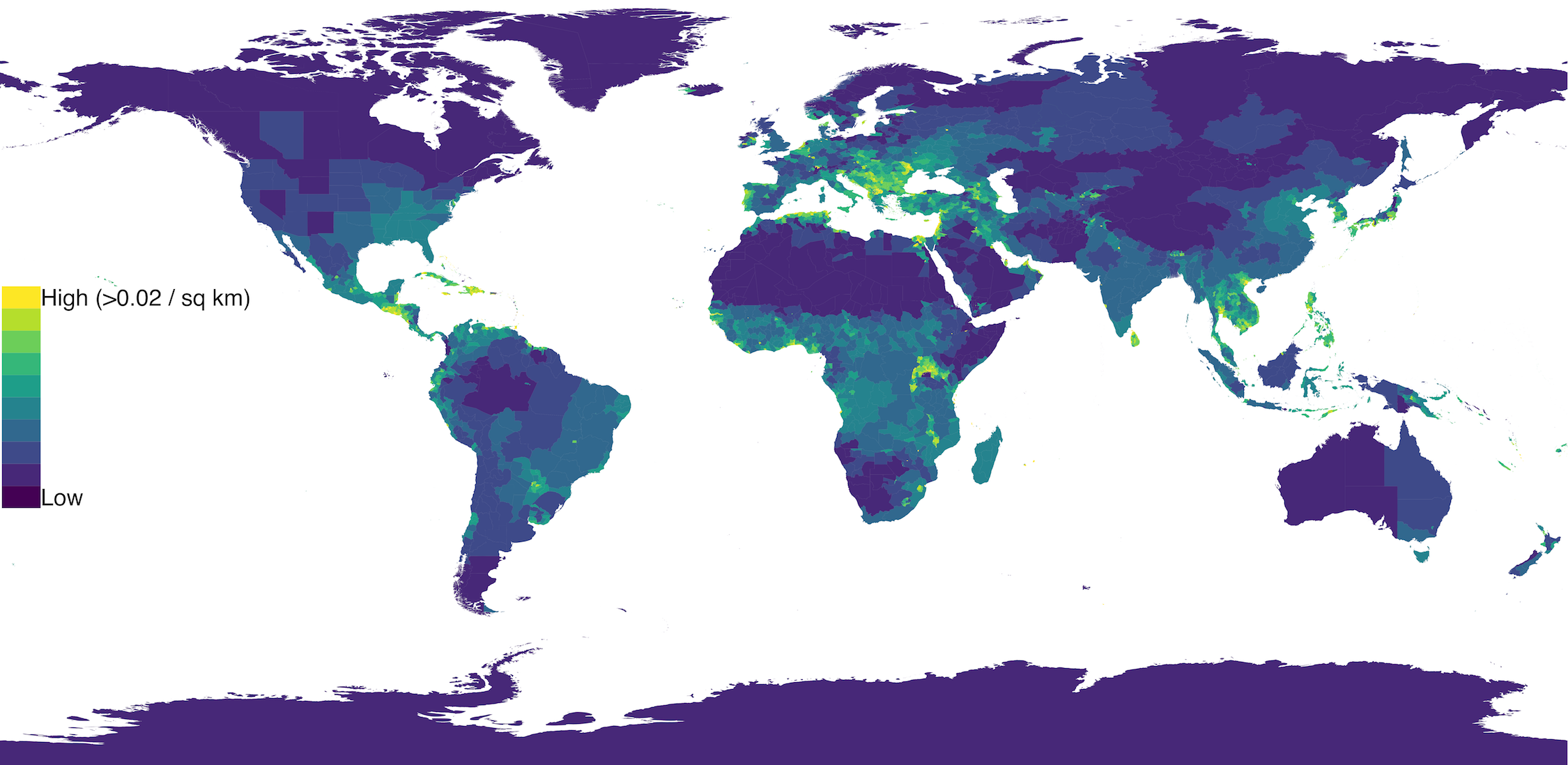
Figure 4: NASA VIIRS fire clusters. Map of log transformed frequency of NASA VIIRS fire clusters per sq km for the time period July 2016 to July 2017. The weekly clustering of fire points corrects for large wildfires that might otherwise skew this indicator of human presence. Fire clusters are more frequent in the underdeveloped regions of the tropics. No correction for gas flares, and other industrial fires, such as steel production has been made. This explains the fire cluster frequency in some of northern areas (data available at [Hic17]).

Call:
lm(formula = log(province_num_weekly_fire_clusters + 1) ~ +log_province_road_area_2 +
    province_pa_area + province_pa_area_Iab_II + province_nightlight)

Residuals:
    Min      1Q  Median      3Q     Max
-5.5262 -0.4897  0.1513  0.6531  4.6418

Coefficients:
                           Estimate Std. Error t value Pr(>|t|)
(Intercept)              -8.017e+00  1.772e-01 -45.234  < 2e-16 ***
log_province_road_area_2  5.263e-01  8.221e-03  64.014  < 2e-16 ***
province_pa_area          5.443e-12  8.216e-13   6.625 4.00e-11 ***
province_pa_area_Iab_II  -6.999e-12  2.772e-12  -2.524   0.0116 *
province_nightlight      -7.362e-03  1.281e-03  -5.745 9.93e-09 ***
---
Signif. codes:  0 *** 0.001 ** 0.01 * 0.05 . 0.1   1

Residual standard error: 0.9763 on 3595 degrees of freedom
  (1 observation deleted due to missingness)
Multiple R-squared:  0.6117,    Adjusted R-squared:  0.6113
F-statistic:  1416 on 4 and 3595 DF,  p-value: < 2.2e-16

Analysis of Variance Table

Response: log(province_num_weekly_fire_clusters + 1)
                           Df Sum Sq Mean Sq   F value    Pr(>F)
log_province_road_area_2    1 5312.3  5312.3 5573.9008 < 2.2e-16 ***
province_pa_area            1   47.9    47.9   50.2485 1.623e-12 ***
province_pa_area_Iab_II     1    5.9     5.9    6.1841   0.01294 *
province_nightlight         1   31.5    31.5   33.0094 9.934e-09 ***
Residuals                3595 3426.3     1.0
---
Signif. codes:  0 *** 0.001 ** 0.01 * 0.05 . 0.1   1

Caveats:  industrial fires are mixed in (no correction for gas flares). We presume the artisanal fires to dominate

Indicator of Remoteness

As an indicator of remoteness, we propose to extend the travel time to major cities dataset (Nelson 2008) by the Mapbox Directions (mapbox.com 2017) mean travel time from the province centre point (centroid) to capitals ([Rud18]), airports ([Nat17, Our]), and seaports ([Age]), as more remote places are likely understudied.

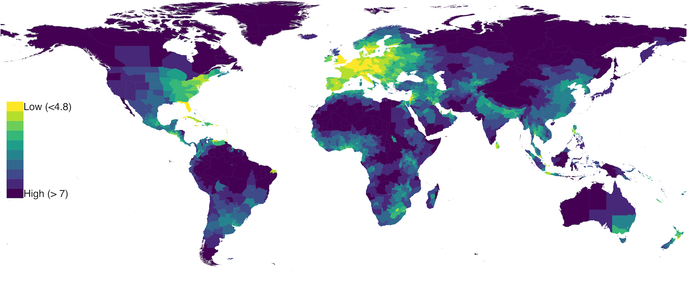
Figure 5: Log transformed average travel times. Map illustrating log transformed average travel time from the province central point to the closest settlement over 50,000 inhabitants, to the three spatially closest capital cities, ports and airports. For large neighboring states, such as Russia, China, India, Brazil, Canada, and the United States of America the distance to the capital city has a very strong impact, representing the governance aspects of remoteness (data available at [Hic17]).

The Remoteness Index is the log transformed average (omitting NAs) of the mean travel time from the province centre point (the centroid as calculated by R package sf function st_centroid) to the closest settlement over 50,000 inhabitants, and the travel times to the three spatially closest capital cities (legislative centres), airports (accessibility), and seaports (supply chain) by linking the osrm R-package ([Gir19]) to the Mapbox Distance API ([Map]). In order to validate this remoteness index, we test the hypothesis that larger areas with less nightlight, and less roads are more remote (R²= 0.45, 3595 df; see model output below; see Fig 5).

Call:
lm(formula = log(province_remoteness_min + 1) ~ +log_province_area_m2 +
    log_province_road_area_2 + province_nightlight)

Residuals:
    Min      1Q  Median      3Q     Max
-2.5618 -0.4290 -0.0708  0.3650  3.3375

Coefficients:
                           Estimate Std. Error t value Pr(>|t|)
(Intercept)               4.9857188  0.1199225   41.57   <2e-16 ***
log_province_area_m2      0.3785360  0.0118679   31.90   <2e-16 ***
log_province_road_area_2 -0.3409079  0.0135638  -25.13   <2e-16 ***
province_nightlight      -0.0184455  0.0009732  -18.95   <2e-16 ***
---
Signif. codes:  0 *** 0.001 ** 0.01 * 0.05 . 0.1   1

Residual standard error: 0.6698 on 3595 degrees of freedom
  (2 observations deleted due to missingness)
Multiple R-squared:  0.4529,    Adjusted R-squared:  0.4524
F-statistic:   992 on 3 and 3595 DF,  p-value: < 2.2e-16

Analysis of Variance Table

Response: log(province_remoteness_min + 1)
                           Df  Sum Sq Mean Sq F value    Pr(>F)
log_province_area_m2        1  746.93  746.93 1664.77 < 2.2e-16 ***
log_province_road_area_2    1  427.08  427.08  951.89 < 2.2e-16 ***
province_nightlight         1  161.18  161.18  359.25 < 2.2e-16 ***
Residuals                3595 1612.95    0.45
---
Signif. codes:  0 *** 0.001 ** 0.01 * 0.05 . 0.1   1

Caveats: the travel times for low traffic reported roads/little driven roads, (etc in Central Africa) are very optimistic (eg 14 hours instead of 40 from Chinko to Bangui) because the political condition (road blocks) are not documented.

Indicator of Scientific Knowledge/Publications

As an indicator for scientific field sampling effort, we query the Web of Science SCI and SSCI catalogues for country and province names in various languages. We used the R-package rwos ([Bar19]) to query the Web of Science Lite API ([Reu12]); country and province name were taken from the GADM v.2.8 dataset ([GAD]) and the R-package countrycode ([Are19]), and results were filtered for the Web of Science category biodiversity and conservation.

This method is not aiming to quantify the actual number of publications per province, but works as a relative index of scientific attention. The scope of these queries is 1993 to 2016 - starting with the United Nations Earth Summit conference in Rio de Janeiro.

All queries and the result total have been retrieved and stored with the help of the R script available in  [Hic17a] and allows for reproduction for any institution that holds Web of Science access.

To obtain information on those provinces, that have only very few mentions since 1993, we infer a conservation publication estimate, based on the proportion of biodiversity and conservation results to those for the country overall, and multiplied by the overall number of publications for that province. If a country has a total of N publications and C conservation publications, and x publications for a province, the inferred publication density (IPD) is calculated as IPD=(C/N)*x.

We note that countries appear to have a reputation for a certain research topic that appears to be rather stable over time (a certain inertia effect). We do use the IPD instead of simply the number of biodiversity and conservation category WoS publications by province, as we’d then have to neglect the detail within the more underrepresented provinces.

We checked the inferred result by multiplying the provincial result across all categories, which correlates strongly with the actual number of conservation related publications (R²=0.98, 3596 df; see below).

Call:
lm(formula = province_wos_cons_inferred ~ province_wos_cons)

Residuals:
    Min      1Q  Median      3Q     Max
-797.80    0.95    1.00    1.29  368.07

Coefficients:
                   Estimate Std. Error t value Pr(>|t|)
(Intercept)       -0.948379   0.352278  -2.692  0.00713 **
province_wos_cons  0.891525   0.002339 381.235  < 2e-16 ***
---
Signif. codes:  0 *** 0.001 ** 0.01 * 0.05 . 0.1   1

Residual standard error: 21.03 on 3596 degrees of freedom
  (3 observations deleted due to missingness)
Multiple R-squared:  0.9759,    Adjusted R-squared:  0.9758
F-statistic: 1.453e+05 on 1 and 3596 DF,  p-value: < 2.2e-16

Analysis of Variance Table

Response: province_wos_cons_inferred
                    Df   Sum Sq  Mean Sq F value    Pr(>F)
province_wos_cons    1 64248196 64248196  145340 < 2.2e-16 ***
Residuals         3596  1589630      442
---
Signif. codes:  0 *** 0.001 ** 0.01 * 0.05 . 0.1   1

In a linear mixed model correcting for country as random effect (see details below), this inferred conservation index is positively explained most strongly by the countries’ life expectancy at birth (estim. =1.446e-02 , p = 0.015), the nightlight index (estim. =1.699e-02 , p = 2e-16), and the logistic area of buffered roads (estim. =1.415e-01 , p = 2e-16).

Linear mixed model fit by REML t-tests use Satterthwaite approximations to
  degrees of freedom [lmerMod]
Formula: log(province_wos_cons_inferred + 1) ~ +province_pa_area_count +
    province_area_species_count + province_pa_area_Iab_II_count +
    province_nightlight + country_SP.DYN.LE00.IN + log_province_road_area_2 +
    (1 | country_iso)

REML criterion at convergence: 6932.5

Scaled residuals:
    Min      1Q  Median      3Q     Max
-5.2709 -0.4094 -0.1212  0.1968  7.4844

Random effects:
 Groups      Name        Variance Std.Dev.
 country_iso (Intercept) 0.6202   0.7875
 Residual                0.3611   0.6009
Number of obs: 3428, groups:  country_iso, 204

Fixed effects:
                                Estimate Std. Error         df t value Pr(>|t|)
(Intercept)                   -3.496e+00  4.569e-01  3.460e+02  -7.652 1.98e-13
province_pa_area_count         6.530e-04  1.132e-04  3.314e+03   5.770 8.65e-09
province_area_species_count    1.521e-03  4.132e-04  3.290e+03   3.680 0.000237
province_pa_area_Iab_II_count  3.339e-03  5.226e-04  3.333e+03   6.388 1.91e-10
province_nightlight            1.699e-02  1.195e-03  3.411e+03  14.213  < 2e-16
country_SP.DYN.LE00.IN         1.446e-02  5.912e-03  2.020e+02   2.445 0.015330
log_province_road_area_2       1.415e-01  1.188e-02  3.271e+03  11.910  < 2e-16

(Intercept)                   ***
province_pa_area_count        ***
province_area_species_count   ***
province_pa_area_Iab_II_count ***
province_nightlight           ***
country_SP.DYN.LE00.IN        *
log_province_road_area_2      ***
---
Signif. codes:  0 *** 0.001 ** 0.01 * 0.05 . 0.1   1

Correlation of Fixed Effects:
            (Intr) prvnc_p__ prvnc_r__ p___I_ prvnc_ c_SP.D
prvnc_p_r_c  0.101
prvnc_r_sp_ -0.086  0.014
prv___I_II_  0.097 -0.195    -0.118
prvnc_nghtl -0.176 -0.037     0.076    -0.036
c_SP.DYN.LE -0.831 -0.036     0.185    -0.044 -0.091
lg_prvn___2 -0.502 -0.142    -0.259    -0.097  0.406 -0.042
Analysis of Variance Table of type III  with  Satterthwaite
approximation for degrees of freedom
                              Sum Sq Mean Sq NumDF  DenDF F.value    Pr(>F)
province_pa_area_count        12.023  12.023     1 3314.3  33.294 8.651e-09 ***
province_area_species_count    4.892   4.892     1 3290.0  13.546 0.0002365 ***
province_pa_area_Iab_II_count 14.738  14.738     1 3333.1  40.811 1.909e-10 ***
province_nightlight           72.949  72.949     1 3411.4 202.004 < 2.2e-16 ***
country_SP.DYN.LE00.IN         2.159   2.159     1  202.1   5.979 0.0153298 *
log_province_road_area_2      51.229  51.229     1 3270.7 141.860 < 2.2e-16 ***
---
Signif. codes:  0 *** 0.001 ** 0.01 * 0.05 . 0.1   1

The number of protected areas in the provinces is a significant predictor of publication density. It is plausible that this is because this represents research that is done in reserves, and also covers a possible bias that more research being done in protected areas, as highlighted in (Martin, Blossey, and Ellis 2012; Meyer, Weigelt, and Kreft 2016). The fact that the number of species present according to IUCN species range maps (estim.= 8.135e-02, p = 0.0002) also explains the number of publications might, however, reflect a causal relationship in the other direction – i.e that range maps are themselves an artefact of a spatial publication frequency bias.

For model explanation, and statistical analysis, the R-packages lme4, lmerTest and vegan (Bates et al. 2015; Kuznetsova, Bruun Brockhoff, and Haubo Bojesen Christensen 2016; Oksanen et al. 2017) were used.

Caveats: SCI + SSCI is dominated by Western literatures; also we use the former country names, and the current name in seven languages (“de”,“ar”,“fr”,“en”,“es”,“ru”,“zh”), but we do not correct for changes in the province names since 1993.

Principal Component Analysis

Having this dataset (n=3638) on the province level available, we use the R built-in function prcomp to run a principal component analysis, and characterise the provinces with the variables defined earlier (see Table 3).

Table 3: Attributes used in the Principal Component Analysis

Attribute	Timespan	Aggregation Method	Reason	Sources
Province.Area	2017	Sum	To correct for polygon size	[GAD]; levels: 0, 1
Temperature	1970-2000	Mean (omitting Nas)	Possible biodiversity	[FH17]; band: 1
Precipitation	1970-2000	Mean (omitting Nas)	Possible biodiversity	[FH17]; band: 12
Publications	1993-2016	Log-transformed sum	Scientific Knowledge	[Reu12]; catalogues: SCI, SSCI
Fire.Clusters	Jul 2016-Jun 17 (1 year)	Log-transformed sum	Human Presence	[NAS]
Remoteness	2008,2017	Log-tr. mean (omit. Nas)	Logistic Cost & Complexity	[Nel08, Map]
Road.Area	2016	Log-transformed sum	Infrastructure	[GAD, Ibi+16]
Life.Expectancy	1960-2010	Mean (omitting Nas)	Development	[Gro]
Night.Light	2013	Mean (omitting Nas)	Economic Activity	[NGD13]

All records are complete on spatially derived attributes, however, the other data columns were often found to be incomplete, which resulted in  reduction of characterised provinces (see run_pca R script available at [Hic17b]; it uses the ggfortify R-package ([THL16] graph).

PCA Results

Running the PCA on the attributes illustrated below the synthetic variables PC1 and PC2 explain more than 54% of the variance (see below). All PCA output and graphics are available at [Hic17c]

Importance of components:
                          PC1    PC2    PC3    PC4     PC5     PC6     PC7
Standard deviation     1.7192 1.3840 1.0873 0.8879 0.86038 0.73650 0.60917
Proportion of Variance 0.3284 0.2128 0.1314 0.0876 0.08225 0.06027 0.04123
Cumulative Proportion  0.3284 0.5412 0.6726 0.7602 0.84242 0.90270 0.94393
                           PC8     PC9
Standard deviation     0.57678 0.41471
Proportion of Variance 0.03696 0.01911
Cumulative Proportion  0.98089 1.00000

Provinces, that had to be dropped due to incomplete information come from 53 countries (n=184; see Table 4) and were mainly incomplete for life expectancy (170 NAs), as well as temperature (27 NAs), precipitation (24 NAs), remoteness (3 NAs), and inferred publications (3 NAs). Most of these provinces are ex-colonial small islands where the World Bank datasets do not record Life Expectancy. There is also no life expectancy data for Antarctica, Western Sahara, and Kosovo.

Table 4: Provinces that were dropped before the PCA as of NA values are largely formerly colonial islands, where Life expectancy is documented together with the mainland counterpart. Table not included here due to volume; available at [Hic17c] in dropped_provinces.csv

Table 5: Scaled input to the PCA (without NAs) – first 20 rows. All 3602 records available at [Hic17c] in pca_input_scaled.csv

Area	Temp	Precip	Public.	Road	Fire	Life	Light	Remote	Name
-0.14	1.03	1.96	0.46	0.36	0.1	-0.79	-0.58	3.63	Andaman and Nicobar IND 1
0.49	1.13	-0.42	1.92	1.47	1.8	-0.79	-0.16	0.64	Andhra Pradesh IND 2
0.17	-0.44	0.8	0.77	0.7	1.12	-0.79	-0.63	1.16	Arunachal Pradesh IND 3
0.15	0.69	1.48	1.4	1.22	1.37	-0.79	-0.43	0.33	Assam IND 4
0.22	0.9	-0.08	1.21	1.42	1.21	-0.79	-0.43	0.09	Bihar IND 5
-0.17	0.72	-0.26	0.58	-1.12	-1.02	-0.79	3.85	0.42	Chandigarh IND 6
0.39	0.91	0.18	0.41	1.11	1.62	-0.79	-0.36	0.56	Chhattisgarh IND 7
-0.16	0.99	1.43	-0.62	-1.14	-0.27	-0.79	0.91	0.44	Dadra and Nagar Haveli IND 8
-0.17	1.02	0.4	-0.63	-1.27	-0.76	-0.79	2.75	1.06	Daman and Diu IND 9
-0.15	1.06	2.08	0.91	0.23	0.48	-0.79	0.32	0.4	Goa IND 10
0.59	1.05	-0.63	1.74	1.7	1.75	-0.79	-0.19	0.95	Gujarat IND 11
0.01	0.82	-0.77	0.99	1.3	1.17	-0.79	0.57	0.38	Haryana IND 12
0.06	-1.16	-0.12	1.18	0.97	0.9	-0.79	-0.44	1.07	Himachal Pradesh IND 13
0.26	-1.96	-0.92	0.49	1.11	0.81	-0.79	-0.55	1.46	Jammu and Kashmir IND 14
0.16	0.84	0.05	0.59	1.04	1.28	-0.79	-0.44	0.03	Jharkhand IND 15
0.61	0.87	-0.04	1.92	1.99	1.78	-0.79	-0.15	0.65	Karnataka IND 16
-0.01	0.94	1.98	2.03	1.24	0.92	-0.79	0.02	0.79	Kerala IND 17
-0.17	1.15	0.77	0.02	-1.67	-1.91	-0.79	-0.29	0.81	Lakshadweep IND 18
1.09	0.87	-0.18	1.16	1.63	2.08	-0.79	-0.44	0.49	Madhya Pradesh IND 19

The rotational matrix resulting from the PCA is indicated in the block below.

                             PC1         PC2         PC3         PC4
Province.Area                0.3318507  0.16119946 -0.23316526  0.60370130
Temperature                 -0.1528287 -0.49549426 -0.43369167 -0.25613610
Precipitation               -0.2054726 -0.28692870 -0.58012590  0.29654050
Publications                 0.2387599  0.31759411 -0.55359429 -0.06113565
Road.Area                    0.4963806  0.17453185 -0.04811661 -0.28960205
Fire.Clusters                0.4672544 -0.03833896 -0.20032359 -0.43068460
Life.Expectancy             -0.1792966  0.56012284 -0.11065538  0.16897863
Night.Light                 -0.3526410  0.31002747 -0.21099537 -0.18497600
log_province_remoteness_min  0.3821910 -0.32174555  0.12379177  0.38227835
                             PC5        PC6        PC7         PC8
Province.Area               -0.471584229  0.3927448 -0.2447083 -0.08491258
Temperature                 -0.269149264  0.1416724 -0.1689974  0.55908783
Precipitation                0.482472067  0.1330648  0.2387677 -0.37468527
Publications                 0.012939285 -0.6776335 -0.2358452  0.04205512
Road.Area                    0.204684559  0.1506349  0.1018911 -0.06788357
Fire.Clusters                0.003254859  0.3674552  0.2494079 -0.05224260
Life.Expectancy              0.341788717  0.2659446  0.1906336  0.62006840
Night.Light                 -0.555636938 -0.0381395  0.5729529 -0.20694841
log_province_remoteness_min -0.069007042 -0.3448068  0.6014337  0.32156342
                             PC9
Province.Area               -0.03655290
Temperature                 -0.20924377
Precipitation               -0.05555159
Publications                 0.12319613
Road.Area                   -0.74658140
Fire.Clusters                0.59549747
Life.Expectancy              0.07031861
Night.Light                 -0.13965107
log_province_remoteness_min -0.01301993

An excerpt of principal component coordinates for the lower right quadrant of the PC1 and PC2 plot, are indicated in Table 6. The score used to rank the provinces is composed of the absolute value of the PC1 plus the absolute value of PC2 coordinates.

Table 6: Principal component coordinates for the lower right quadrant of the PC1 and PC2 plot. Score is the sum of absolute PC1 plus absolute PC2 – first 20 rows. All records are available at [Hic17c] in pca_bottom_right.csv

	PC1	PC2	PC3	PC4	PC5	PC6	PC7	PC8	PC9
Andaman and Nicobar IND 1	1.35	-2.71	-1.18	1.42	0.64	-1.4	1.98	0.66	-0.5
Andhra Pradesh IND 2	2.71	-0.18	-1.8	-1.09	-0.81	-0.42	-0.22	0.34	-0.09
Arunachal Pradesh IND 3	1.83	-0.64	-0.69	0.25	0.5	-0.46	0.54	-0.64	0.3
Assam IND 4	1.69	-0.78	-2.16	-0.53	0.61	-0.19	0.1	-0.59	-0.17
Bihar IND 5	1.9	-0.36	-1.27	-1.05	-0.19	-0.14	-0.46	0.01	-0.43
Chhattisgarh IND 7	1.94	-0.86	-1.07	-0.66	-0.36	0.51	0.11	-0.0	-0.05
Gujarat IND 11	3.0	-0.17	-1.54	-0.93	-0.93	-0.35	-0.08	0.45	-0.3
Haryana IND 12	1.55	-0.05	-0.78	-1.46	-0.94	-0.41	0.25	0.15	-0.45
Jharkhand IND 15	1.51	-0.65	-0.94	-0.95	-0.15	0.24	-0.32	-0.07	-0.13
Karnataka IND 16	3.01	-0.02	-1.99	-0.92	-0.56	-0.24	-0.08	0.01	-0.5
Kerala IND 17	1.4	-0.88	-2.8	-0.37	0.66	-0.99	0.51	-0.51	-0.53
Madhya Pradesh IND 19	3.13	-0.21	-1.67	-0.44	-0.94	0.73	-0.35	-0.03	-0.1
Maharashtra IND 20	3.22	-0.09	-2.11	-0.54	-0.97	0.5	-0.21	-0.08	-0.3
Manipur IND 21	0.85	-0.91	-0.76	-0.03	0.54	-0.5	0.04	-0.41	-0.16
Meghalaya IND 22	0.44	-1.57	-2.47	0.39	1.68	-0.06	0.53	-1.33	-0.09
Mizoram IND 23	0.75	-1.45	-1.09	0.15	0.82	-0.17	0.38	-0.44	-0.33
Nagaland IND 24	0.67	-1.19	-0.45	0.17	0.53	-0.29	0.29	-0.38	-0.02
Odisha IND 26	2.19	-0.74	-1.33	-0.74	-0.3	0.55	-0.03	-0.06	-0.15
Tamil Nadu IND 31	2.81	-0.16	-1.88	-1.19	-0.75	-0.66	0.21	0.36	-0.47

The top 100 ranking provinces are aggregated by country in Table 7 and in detail listed in Table 8. We manually checked all provinces omitted from the PCA to confirm that they would not have made the priority list in terms of remoteness, area, fire and publications.

Table 7: Top 100 provinces according to PCA lower left quadrant score aggregated by country.

Country	Number of Provinces in Top 100
Angola	12
South Sudan	10
Chad	8
Ethiopia	8
Mozambique	8
Somalia	8
Central African Republic	7
Democratic Republic of the Congo	7
Mali	7
Niger	5
Zambia	5
Brazil	3
Sudan	3
Bolivia	2
Madagascar	2
Eritrea	1
India	1
Nigeria	1
Peru	1
Tanzania	1

Table 8: Top 100 provinces according to PCA lower right quadrant score - first 20 rows. All records are available at [Hic17c] in top100 detail.csv

Country	ID	Province	Area (m2)	Temp.	Precip.	Pub.	Road.Area
Tanzania	22	Ruvuma	63075882644.83	296.13	1184.87	0.45	22.81
Central African Republic	1	Bamingui-Bangoran	58468947111.12	299.4	1152.17	0	21.15
Central African Republic	4	Haut-Mbomou	56355703351.32	298.12	1435.35	0	21.1
Central African Republic	5	Haute-Kotto	86049245472.47	297.62	1316.04	0.01	21.6
Central African Republic	9	Mbomou	60150494915.11	297.75	1618.5	0.01	21.55
Madagascar	4	Mahajanga	151672635669.44	297.98	1486.65	1.75	22.87
Central African Republic	13	Ouaka	49209480500.37	297.66	1451.32	0.01	21.78
Madagascar	6	Toliary	164030931907.8	297.16	832.04	0.82	23.9
Central African Republic	15	Ouham	52964954181.79	298.75	1330.14	0.04	22.42
Sudan	8	North Darfur	317200633021.61	298.54	147.53	0.12	21.81
Central African Republic	17	Vakaga	46696061043.21	299.37	886.35	0	21.91
Chad	2	Batha	90412921603.27	302.74	290.92	0	21.56
Chad	3	Borkou	256248321053.96	299.67	30.26	0.04	21.16
Chad	4	Chari-Baguirmi	46030941104.07	301.6	690.07	0.04	21.3
Sudan	14	South Darfur	78133459700.04	299.37	651.31	0.22	21.87
Chad	7	Guéra	61038076376.23	301.65	734.91	0.05	21.96
Peru	17	Loreto	375548002886.75	299.26	2525.32	1.44	21.65
Sudan	17	West Kurdufan	112959212480.54	300.43	491.84	0.11	22.66
Chad	10	Lac	19842923740.3	300.96	262.83	0.02	22.3

References

- [Aeb+15] T. Aebischer, R. Hickisch, J. Woolgar and E. Do Linh San “Dologale dybowskii. The IUCN Red List of Threatened Species 2015: e. T41598A45205821”, 2015
- [Age] National Geospatial Intelligence Agency “World Port Index National Geospatial Intelligence Agency” URL: https://msi.nga.mil/NGAPortal/MSI.portal?_nfpb=true&_pageLabel=msi_portal_page_62&pubCode=0015
- [Ahr+11] Antje Ahrends et al. “Funding begets biodiversity: Funding begets biodiversity” In Diversity and Distributions 17.2, 2011, pp. 191–200 DOI: 10.1111/j.1472-4642.2010.00737.x
- [Ara+11] Silvia C. Aranda et al. “Designing a survey protocol to overcome the Wallacean shortfall: a working guide using bryophyte distribution data on Terceira Island (Azores)” In The Bryologist 114.3, 2011, pp. 611–624 DOI: 10.1639/0007-2745-114.3.611
- [Are19] Vincent Arel-Bundock “R package: Convert country names and country codes. Assigns region descriptors.: vincentarelbundock/countrycode” original-date: 2011-08-17T20:33:13Z, 2019 URL: https://github.com/vincentarelbundock/countrycode
- [AS13] T. Amano and W.. Sutherland “Four barriers to the global understanding of biodiversity conservation: wealth, language, geographical location and security” In Proceedings of the Royal Society B: Biological Sciences 280.1756, 2013, pp. 20122649–20122649 DOI: 10.1098/rspb.2012.2649
- [BAD11] E… Brooks, David James Allen and William RT Darwall “The status and distribution of freshwater biodiversity in central Africa” IUCN, 2011
- [Bar19] Julien Barnier “R interface to Web of Science Web Services API. Contribute to juba/rwos development by creating an account on GitHub” original-date: 2017-05-11T08:19:50Z, 2019 URL: https://github.com/juba/rwos
- [BCS15] David Brugière, Bertrand Chardonnet and Paul Scholte “Large-Scale Extinction of Large Carnivores (Lion Panthera Leo , Cheetah Acinonyx Jubatus and Wild Dog Lycaon Pictus ) in Protected Areas of West and Central Africa” In Tropical Conservation Science 8.2, 2015, pp. 513–527 DOI: 10.1177/194008291500800215
- [Boa+10] Elizabeth H. Boakes et al. “Distorted Views of Biodiversity: Spatial and Temporal Bias in Species Occurrence Data” In PLoS Biology 8.6, 2010, pp. e1000385 DOI: 10.1371/journal.pbio.1000385
- [Bou+10] Philippe Bouché et al. “Has the final countdown to wildlife extinction in Northern Central African Republic begun?: Wildlife extinction Central African Republic” In African Journal of Ecology 48.4, 2010, pp. 994–1003 DOI: 10.1111/j.1365-2028.2009.01202.x
- [Bri10] Daniel Brito “Overcoming the Linnean shortfall: Data deficiency and biological survey priorities” In Basic and Applied Ecology 11.8, 2010, pp. 709–713 DOI: 10.1016/j.baae.2010.09.007
- [Bro+14] Zoe M. Brooke, Jon Bielby, Kate Nambiar and Chris Carbone “Correlates of Research Effort in Carnivores: Body Size, Range Size and Diet Matter” In PLoS ONE 9.4, 2014, pp. e93195 DOI: 10.1371/journal.pone.0093195
- [Bro09] Jedediah F. Brodie “Is research effort allocated efficiently for conservation? Felidae as a global case study” In Biodiversity and Conservation 18.11, 2009, pp. 2927–2939 DOI: 10.1007/s10531-009-9617-3
- [Can15] Peter Canby “Elephant Watch” In The New Yorker 91, 2015, pp. 34
- [CGM17] Abu Conteh, Michael C. Gavin and Joe McCarter “Assessing the impacts of war on perceived conservation capacity and threats to biodiversity” In Biodiversity and Conservation 26.4, 2017, pp. 983–996 DOI: 10.1007/s10531-016-1283-7
- [Col08] Paul Collier “The bottom billion: Why the poorest countries are failing and what can be done about it” Oxford University Press, USA, 2008
- [DMN11] Paul De Ornellas, E.J. Milner-Gulland and Emily Nicholson “The impact of data realities on conservation planning” In Biological Conservation 144.7, 2011, pp. 1980–1988 DOI: 10.1016/j.biocon.2011.04.018
- [DP18] Joshua H. Daskin and Robert M. Pringle “Warfare and wildlife declines in Africa’s protected areas” In Nature 553.7688, 2018, pp. 328–332 DOI: 10.1038/nature25194
- [Eng+15] Kristine Engemann et al. “Limited sampling hampers “big data” estimation of species richness in a tropical biodiversity hotspot” In Ecology and Evolution 5.3, 2015, pp. 807–820 DOI: 10.1002/ece3.1405
- [Fay07] J. Fay “Ivory wars: Last stand in Zakouma” In National geographic 211.3, 2007, pp. 34–65
- [FFL05] I. Fazey, J. Fischer and D.B. Lindenmayer “What do conservation biologists publish?” In Biological Conservation 124.1, 2005, pp. 63–73 DOI: 10.1016/j.biocon.2005.01.013
- [FH17] Stephen E. Fick and Robert J. Hijmans “WorldClim 2: new 1-km spatial resolution climate surfaces for global land areas” In International Journal of Climatology 37.12, 2017, pp. 4302–4315
- [Fis+11] Rebecca Fisher et al. “Global mismatch between research effort and conservation needs of tropical coral reefs” In Conservation Letters 4.1, 2011, pp. 64–72
- [Fou19] Open Source Geospatial Foundation “GDAL is an open source X/MIT licensed translator library for raster and vector geospatial data formats.: OSGeo/gdal” original-date: 2012-10-09T21:39:58Z, 2019 URL: https://github.com/OSGeo/gdal
- [GAD] GADM “GADM database of Global Administrative Areas.” URL: https://gadm.org/
- [Gas00] Kevin J. Gaston “Global patterns in biodiversity” In Nature 405.6783, 2000, pp. 220–227 DOI: 10.1038/35012228
- [Gay+16] Kaitlyn M Gaynor et al. “War and wildlife: linking armed conflict to conservation” In Frontiers in Ecology and the Environment 14.10, 2016, pp. 533–542 DOI: 10.1002/fee.1433
- [Gir19] Timothée Giraud “Shortest Paths and Travel Time from OpenStreetMap with R: rCarto/osrm” original-date: 2015-09-11T07:39:33Z, 2019 URL: https://github.com/rCarto/osrm
- [Gre+06] Richard Grenyer et al. “Global distribution and conservation of rare and threatened vertebrates” In Nature 444.7115, 2006, pp. 93–96 DOI: 10.1038/nature05237
- [Gro] World Bank Group “Life expectancy at birth, total (years) — Data” URL: https://data.worldbank.org/indicator/SP.DYN.LE00.IN
- [HA13] Raffael Hickisch and Thierry Aebischer “An Update On African Elephant Loxodonta Africana In The Chinko/Mbari Drainage Basin, Central African Republic”, 2013 DOI: 10.5281/zenodo.997977
- [Hic] Raffael Hickisch “Data used for Web of Science World Conservation Publication Index 1993 - 2016 — Biodiversity Publication Bias Compromises Setting Conservation Priorities — Zenodo” URL: https://zenodo.org/record/893910#.XGcphspm2jk
- [Hic17] Raffael Hickisch “Aggregated Spatial Data by province GPKG Format — Biodiversity Publication Bias Compromises Setting Conservation Priorities”, 2017 DOI: 10.5281/zenodo.998818
- [Hic17a] Raffael Hickisch “R script to prepare a Web of Science based conservation index” original-date: 2017-09-17T21:31:04Z, 2017 URL: https://github.com/raffael-hickisch/rwosconsindex
- [Hic17b] Raffael Hickisch “R script to process vector data on the province level worldwide” original-date: 2017-09-28T13:57:06Z, 2017 URL: https://github.com/raffael-hickisch/provincer
- [Hic17c] Raffael Hickisch “Supplementary Material PCA — Biodiversity Publication Bias Compromises Setting Conservation Priorities”, 2017 DOI: 10.5281/zenodo.998889
- [Hil04] Helmut Hillebrand “On the Generality of the Latitudinal Diversity Gradient” In The American Naturalist 163.2, 2004, pp. 192–211 DOI: 10.1086/381004
- [Ibi+16] Pierre L. Ibisch et al. “A global map of roadless areas and their conservation status” In Science 354.6318, 2016, pp. 1423–1427 DOI: 10.1126/science.aaf7166
- [IUC] IUCN “IUCN Red List of Threatened Species Spatial Data Download” URL: https://www.iucnredlist.org/resources/spatial-data-download
- [JMG12] Walter Jetz, Jana M. McPherson and Robert P. Guralnick “Integrating biodiversity distribution knowledge: toward a global map of life” In Trends in Ecology & Evolution 27.3, 2012, pp. 151–159 DOI: 10.1016/j.tree.2011.09.007
- [Kra+13] Stephanie Kramer-Schadt et al. “The importance of correcting for sampling bias in MaxEnt species distribution models” In Diversity and Distributions 19.11, 2013, pp. 1366–1379 DOI: 10.1111/ddi.12096
- [Lob08] Jorge M. Lobo “Database records as a surrogate for sampling effort provide higher species richness estimations” In Biodiversity and Conservation 17.4, 2008, pp. 873–881 DOI: 10.1007/s10531-008-9333-4
- [Man+14] Philip D. Mannion, Paul Upchurch, Roger B.J. Benson and Anjali Goswami “The latitudinal biodiversity gradient through deep time” In Trends in Ecology & Evolution 29.1, 2014, pp. 42–50 DOI: 10.1016/j.tree.2013.09.012
- [Map] Mapbox “An introduction to the Mapbox web services APIs.” URL: https://www.mapbox.com/api/
- [MBE12] Laura J Martin, Bernd Blossey and Erle Ellis “Mapping where ecologists work: biases in the global distribution of terrestrial ecological observations” In Frontiers in Ecology and the Environment 10.4, 2012, pp. 195–201 DOI: 10.1890/110154
- [Mey+16] Carsten Meyer et al. “Range geometry and socio-economics dominate species-level biases in occurrence information: Species-level bias in occurrence records” In Global Ecology and Biogeography 25.10, 2016, pp. 1181–1193 DOI: 10.1111/geb.12483
- [Mye+00] Norman Myers et al. “Biodiversity hotspots for conservation priorities” In Nature 403.6772, 2000, pp. 853
- [Nac+14] Janet Nackoney et al. “Impacts of civil conflict on primary forest habitat in northern Democratic Republic of the Congo, 1990–2010” In Biological Conservation 170, 2014, pp. 321–328 DOI: 10.1016/j.biocon.2013.12.033
- [NAS] NASA “VIIRS I-Band 375 m Active Fire Data — Earthdata” URL: https://earthdata.nasa.gov/earth-observation-data/near-real-time/firms/viirs-i-band-active-fire-data
- [Nat17] Natural Earth “Airports v.2.0”, 2017 URL: http://www.naturalearthdata.com/downloads/10m-cultural-vectors/airports/
- [Nel08] Andrew Nelson “Travel time to major cities: A global map of Accessibility”, 2008
- [NGD13] NOAA NGDC “Version 4 DMSP-OLS nighttime lights time series” In National Oceanic and Atmospheric Administration-National Geophysical Data Center, 2013
- [OGC] OGC “OGC GeoPackage” URL: https://www.geopackage.org/
- [Ond+17] Ondoua Gervais Ondoua et al. “An Assessment of Poaching and Wildlife Trafficking in the Garamba-Bili-Chinko Transboundary Landscape”, 2017
- [Our] OurAirports “Airports by popularity @ OurAirports” URL: http://ourairports.com/airports/
- [RD03] Sushma Reddy and Liliana M. Dávalos “Geographical sampling bias and its implications for conservation priorities in Africa: Sampling bias and conservation in Africa” In Journal of Biogeography 30.11, 2003, pp. 1719–1727 DOI: 10.1046/j.1365-2699.2003.00946.x
- [Reu12] Thomson Reuters “Web of Science.”, 2012
- [Roc+11] Duccio Rocchini et al. “Accounting for uncertainty when mapping species distributions: The need for maps of ignorance” In Progress in Physical Geography: Earth and Environment 35.2, 2011, pp. 211–226 DOI: 10.1177/0309133311399491
- [Ron+06] Carlo Rondinini et al. “Tradeoffs of different types of species occurrence data for use in systematic conservation planning: Species data for conservation planning” In Ecology Letters 9.10, 2006, pp. 1136–1145 DOI: 10.1111/j.1461-0248.2006.00970.x
- [Rud18] boB Rudis “Tools to Work With the OpenStreetMap (OSM) Overpass API in R: hrbrmstr/overpass” original-date: 2015-08-10T15:21:18Z, 2018 URL: https://github.com/hrbrmstr/overpass
- [SL09] Pablo Sastre and Jorge M. Lobo “Taxonomist survey biases and the unveiling of biodiversity patterns” In Biological Conservation 142.2, 2009, pp. 462–467 DOI: 10.1016/j.biocon.2008.11.002
- [Str16] Christian Strobl “PostGIS” In Encyclopedia of GIS Cham: Springer International Publishing, 2016, pp. 1–8 DOI: 10.1007/978-3-319-23519-6˙1012-2
- [Sut+12] William J. Sutherland et al. “A horizon scanning assessment of current and potential future threats to migratory shorebirds” In Ibis 154.4, 2012, pp. 663–679
- [THL16] Yuan Tang, Masaaki Horikoshi and Wenxuan Li “ggfortify: Unified Interface to Visualize Statistical Results of Popular R Packages” In The R Journal 8.2, 2016, pp. 474 DOI: 10.32614/RJ-2016-060
- [Tyd+16] Laura Tydecks et al. “Biological Field Stations: A Global Infrastructure for Research, Education, and Public Engagement” In BioScience 66.2, 2016, pp. 164–171 DOI: 10.1093/biosci/biv174
- [WDP] WDPA “Protected Planet is the online interface for the World Database on Protected Areas (WDPA), and the most comprehensive global database on terrestrial and marine protected areas.” URL: https://www.protectedplanet.net/c/world-database-on-protected-areas
- [Wil+16] Kerrie A. Wilson et al. “Conservation Research Is Not Happening Where It Is Most Needed” In PLOS Biology 14.3, 2016, pp. e1002413 DOI: 10.1371/journal.pbio.1002413
- [YMK13] Wenjing Yang, Keping Ma and Holger Kreft “Geographical sampling bias in a large distributional database and its effects on species richness-environment models” In Journal of Biogeography 40.8, 2013, pp. 1415–1426 DOI: 10.1111/jbi.12108