Meta-analysis of Bayesian analyses

Abstract

Meta-analysis aims to combine results from multiple related statistical analyses. While the natural outcome of a Bayesian analysis is a posterior distribution, Bayesian meta-analyses traditionally combine analyses summarized as point estimates, often limiting distributional assumptions. In this paper, we develop a framework for combining posterior distributions, which builds on standard Bayesian inference, but using distributions instead of data points as observations. We show that the resulting framework preserves basic theoretical properties, such as order-invariance in successive updates and posterior concentration. In addition to providing a consensus analysis for multiple Bayesian analyses, we highlight the benefit of being able to reuse posteriors from computationally costly analyses and update them post-hoc without having to rerun the analyses themselves. The wide applicability of the framework is illustrated with examples of combining results from likelihood-free Bayesian analyses, which would be difficult to carry out using standard methodology.

1 Introduction

Meta-analysis is a term used broadly for a collection of approaches which aim to combine results from multiple related statistical analyses. In the standard formulation, these results are summary statistics computed from data, a typical example being point estimates for the effect size of some treatment. For the combination of point estimates, there exists well-established Bayesian methodology and a large body of literature (see e.g. Higgins et al., 2009, and references therein). However, while the natural outcome of a Bayesian analysis is a posterior distribution, the analogous task of combining posterior distributions has received little attention. In the frequentist paradigm, Xie et al. (2011) have previously introduced a framework for the combination of confidence distributions, a concept loosely related to Bayesian posteriors. In this paper, we develop a Bayesian framework for combining posterior distributions.

In the standard setting of Bayesian random effects meta-analysis, a summary statistic (or data set) $D_{j}$, $j=1,\ldots,J$, has been observed for each of $J$ studies. The summary statistics aim to provide information about some quantity or ‘effect’ of interest. To reflect the general idea of the studies being non-identical but related, it is common to regard them as exchangeable (Gelman et al., 2013), with the study-specific effect represented by some parameter, say $\theta_{j}$, and the overall effect by another parameter, say $\varphi$. This leads to the following hierarchical model:

$$\varphi \sim Q$$

$$\theta_{j} \sim P_{\varphi}$$

$$D_{j} \sim F_{\theta_{j}},$$

where $F_{\theta_{j}}$ is typically modeled as $D_{j}\sim\mathcal{N}(\theta_{j},\hat{\sigma}_{j}^{2}),$ with $\hat{\sigma}_{j}^{2}$ estimated from data. One of the primary goals of the above model is to estimate the overall effect $\varphi$, for which the marginal posterior density is given by

$$q(\varphi|D_{1},\ldots,D_{J})\propto\prod_{j=1}^{J}\left[\int f(D_{j}|\theta_{j})p(\theta_{j}|\varphi)d\theta_{j}\right]q(\varphi).$$ (1)

There are many compelling reasons for reporting analysis results as posterior distributions instead of data summaries, and subsequently combining them in a meta-analysis. First, a distribution describes the analyst’s uncertainty in the obtained results. Second, a posterior distribution can be directly specified on a quantity of interest, whereas a summary statistic often only provides indirect information about the quantity. Furthermore, the posterior distribution may also include prior knowledge not present in the data, but possibly obtained by expert elicitation (e.g. Albert et al., 2012). This is particularly important in problems where not enough data is available to inform a model about some of its parameters. For example, models describing complex biological phenomena may have so many parameters that they cannot be estimated without the use of informative priors (e.g. Kuikka et al., 2014). Thus, the posterior for a given quantity may be primarily informed by its prior and only indirectly by data, which could make the extraction of a meaningful summary statistic challenging. Finally, if we wish to combine the results of such studies in a meta-analysis, it is desirable to preserve the study-specific prior knowledge in the combined model. Unlike data summaries, this knowledge is naturally encapsulated in posterior distributions.

Consider now a setting, where instead of summary statistics $D_{j}$, we have posterior distributions with densities $\pi_{j}(\theta_{j})$ available from each of $J$ studies, based on which we wish to update our prior knowledge about the global effect $\varphi$, in analogy with Equation (1). We build on the interpretation that each $\pi_{j}(\theta_{j})$ is a probabilistic representation of belief (Bernardo and Smith, 1994), which reflects our uncertainty about the value of the corresponding local effect $\theta_{j}$. Updating prior knowledge (in our case regarding $\varphi$) subject to uncertain or ‘soft’ evidence, represented as probability distributions instead of observed values, has been extensively studied as a philosophical topic in both statistics and artificial intelligence. The most well-known of such update rules, Jeffrey’s rule of conditioning (Diaconis and Zabell, 1982; Jeffrey, 2004; Smets, 1993; Zhao and Osherson, 2010), computes the updated probability for an event as a weighted average of the posterior probabilities under all possible values of the evidence. Due to its construction, Jeffrey’s rule is applicable in simple discrete cases but becomes computationally infeasible for more complex models with continuous variables. Instead, we directly marginalize away the uncertainty in the observations as they appear in the likelihood, which leads us to update $q(\varphi)$ as

$$q^{*}(\varphi)\propto\prod_{j=1}^{J}\left[\int p(\theta_{j}|\varphi)\pi_{j}(\theta_{j})d\theta_{j}\right]q(\varphi).$$ (2)

In addition to achieving computational tractability, the above formulation retains some basic properties of standard Bayesian inference, such as order-invariance in successive updates (in contrast with Jeffrey’s rule) and posterior concentration as $J\rightarrow\infty$. From a practical point of view, it is interesting to note that Equations (1) and (2) differ only in the local likelihood $f(D_{j}|\theta_{j})$ being replaced with the density $\pi_{j}(\theta_{j})$. Intuitively, the former carries information provided by the data only, while the latter carries information provided by both the data and additional prior knowledge. A more subtle difference is that in Equation (2), the integration is thought of as being performed with respect to the measure defined by $\pi_{j}$.

Our formulation of the meta-analysis problem also lends itself to an intuitive interpretation as message passing in probabilistic graphical models (Jordan, 2004; Koller and Friedman, 2009). Using the language of undirected models, updating $q(\varphi)$ into $q^{*}(\varphi)$ in Equation (2) is equivalent to propagating beliefs from leaf nodes to the root node in a tree-structured graphical model, with node potentials $q(\varphi)$, $\pi_{j}(\theta_{j})$ and edge potentials $\psi_{j}(\theta_{j},\varphi):=p(\theta_{j}|\varphi)$, $j=1,\ldots,J$, see Figure 1. Further utilizing the induced graphical model structure, we may similarly update any $\pi_{j}(\theta_{j})$ into $\pi_{j}^{*}(\theta_{j})$ by propagating beliefs to the $j$th leaf node from the remaining nodes in the model. This yields a way of updating study-specific posteriors post-hoc, borrowing strength from posteriors obtained in other studies. Besides its intuitive appeal, adopting a graphical model view enables a straightforward extension of the framework to more complex model structures, and it may be utilized in devising efficient computational strategies.

Figure 1: Tree-structured graphical model with study-specific posteriors providing the initial beliefs for $\theta_{1},\ldots,\theta_{J}$.

A major advantage of our meta-analysis framework is its flexibility. In particular, the study-specific inferences resulting in $\pi_{j}(\theta_{j})$ are independent of the combination model, $q(\varphi)\prod_{j=1}^{J}p(\theta_{j}|\varphi)$, which is imposed by the meta-analyst. This means that, unlike in hierarchical models, all study-level complexities are hidden ‘under the hood’ and need not explicitly be included in the meta-analysis. For instance, in likelihood-free models (e.g. Lintusaari et al., 2017; Marin et al., 2012), the data can typically be summarized by a number of different statistics but there is no closed-form likelihood to relate these to the parameter of interest. In our framework, likelihood-free inferences can be conducted separately for each study using approximate Bayesian computation, after which the resulting posteriors are directly combined in a meta-analysis. We highlight the benefit of being able to reuse results from computationally costly analyses, such as likelihood-free inferences, and update them without having to rerun the analyses themselves. In the current paper, we propose a straightforward computational strategy for our framework, where we first impose parametric approximations on the observed posteriors. Sampling from the joint distribution of all variables can then be done using general-purpose software such as Stan (Carpenter et al., 2017). Finally, the obtained joint distribution can be refined using importance sampling, from which any desired marginals can be extracted.

The paper is structured as follows. In Section 2, we develop a framework for conducting Bayesian inference with observed beliefs, which underlies our meta-analysis approach. In Section 3, we summarize the main equations for practical use, and provide further insight into the framework by highlighting connections to message passing in probabilistic graphical models, and standard forms of Bayesian meta-analysis. Section 4 introduces a straightforward computational strategy, which can be implemented using general-purpose software. In Section 5, we illustrate our method with both synthetic and real data. The paper ends with a brief discussion of related work in Section 6 and some concluding remarks in Section 7.

2 Bayesian inference with observed beliefs

In this section, we first develop a posterior update rule given observed beliefs, which is motivated by the problem of conducting meta-analysis for a set of related posterior distributions. The notion of relatedness is here characterized as the exchangeability of the quantities targeted by the posteriors. The proposed update rule is given in Equation (5). We then show in Section 2.1 that this rule retains some basic theoretical properties of standard Bayesian inference.

Let us first assume that $\theta_{1},\ldots,\theta_{J}$ is a collection of observable and exchangeable random quantities. Following standard theory, de Finetti’s representation theorem (e.g. Schervish, 1995) states that if $\theta_{1},\theta_{2},\ldots$ is an infinitely exchangeable sequence of random quantities taking values in a Borel space $(\Theta$, $\mathcal{A})$, then there exists a probability measure $Q$ such that the joint distribution $\mathds{P}$ of the subsequence $\theta_{1},\ldots,\theta_{J}$, i.e. the predictive distribution, has the form

$$\mathds{P}(\theta_{1}\in A_{1},\ldots,\theta_{J}\in A_{J})=\int_{\Phi}\prod_{j=1}^{J}\left[\int_{A_{j}}p(\theta_{j}|\varphi)\lambda(d\theta_{j})\right]Q(d\varphi),$$ (3)

where $A_{1},\ldots,A_{J}\in\mathcal{A}$. Here, the set of probability measures on $\Theta$ is taken to be a family $\{P_{\varphi}|\varphi\in\Phi\}$, indexed by a parameter $\varphi$, such that $Q$ is a probability measure on $\Phi$. Furthermore, we define the density function $p(\cdot|\varphi):=dP_{\varphi}/d\lambda$ with respect to a reference measure $\lambda$ (Lebesgue or counting measure).

In the above standard setting, the Bayesian learning process works through updating $Q$ conditional on observed data. Following Equation (3), the posterior distribution of $\varphi$, given observed values $\theta_{1}=t_{1},\ldots,\theta_{J}=t_{J}$, has the form

$$Q(B|t_{1},\ldots,t_{J})=\frac{\int_{B}\prod_{j=1}^{J}p(t_{j}|\varphi)Q(d\varphi)}{\int_{\Phi}\prod_{j=1}^{J}p(t_{j}|\varphi)Q(d\varphi)},$$ (4)

with $B\in\mathcal{B}$, the Borel $\sigma$-algebra on $\Phi$. We will now build further on this setting, assuming that instead of directly observing the value of each $\theta_{j}$, we have a set of distributions $\Pi_{1},\ldots,\Pi_{J}$, expressing our currently available beliefs about the values of $\theta_{j}$. Note that, while in our current context, we assume that each of the beliefs is obtained as the posterior distribution from a previously conducted analysis, this assumption is not essential to our developments. Importantly, the observed distributions are assumed independent of the distribution we seek to update. In the absence of fixed likelihood contributions $p(t_{j}|\varphi)$ for each observation, we propose to compute the expected likelihood contributions $\int_{\Theta}p(\theta_{j}|\varphi)\Pi_{j}(d\theta_{j})$ with respect to the available beliefs.

The proposed modification of the likelihood now leads to an update of the form

$$Q^{*}(B|\Pi_{1},\ldots,\Pi_{J})=\frac{\int_{B}\prod_{j=1}^{J}\left[\int_{\Theta}p(\theta_{j}|\varphi)\Pi_{j}(d\theta_{j})\right]Q(d\varphi)}{\int_{\Phi}\prod_{j=1}^{J}\left[\int_{\Theta}p(\theta_{j}|\varphi)\Pi_{j}(d\theta_{j})\right]Q(d\varphi)},$$ (5)

where, with slight abuse of notation, we write $Q^{*}(\cdot|\Pi_{1},\ldots,\Pi_{J})$ to denote conditioning on beliefs in analogy with conditioning on fully observed values; we give more context for this choice of notation below in Section 2.1.2. Equation (5) further induces a joint distribution on $\Phi\times\Theta^{J}$, which can be marginalized with respect to $Q$, resulting in a predictive distribution as follows:

$$\mathds{P}^{*}(\theta_{1}\in A_{1},\ldots,\theta_{J}\in A_{J})=\frac{\int_{\Phi}\prod_{j=1}^{J}\left[\int_{A_{j}}p(\theta_{j}|\varphi)\Pi_{j}(d\theta_{j})\right]Q(d\varphi)}{\int_{\Phi}\prod_{j=1}^{J}\left[\int_{\Theta}p(\theta_{j}|\varphi)\Pi_{j}(d\theta_{j})\right]Q(d\varphi)}.$$ (6)

It easy to see that standard Bayesian inference, Equation (4), emerges as a special case of Equation (5) by setting $\Pi_{j}$ to be $\delta_{t_{j}}$, the Dirac measure centered at $t_{j}$. This yields

$$\int_{\Theta}p(\theta_{j}|\varphi)\delta_{t_{j}}(d\theta_{j})=p(t_{j}|\varphi),$$

such that $Q^{*}(\cdot|\delta_{t_{1}},\ldots,\delta_{t_{J}})=Q(\cdot|t_{1},\ldots,t_{J})$. Throughout this work, we assume that $\Pi_{j}$ is a probability measure. However, it is interesting to note that if we make an exception and allow $\Pi_{j}$ to be the Lebesgue (or counting) measure $\lambda$ for all $j$, which corresponds to having a uniformly distributed—possibly improper—belief about the value of $\theta_{j}$, then the updated measure $Q^{*}$ in Equation (5) equals the prior probability measure $Q$. Moreover, with this choice of $\Pi_{j}$, Equation (6) reduces to the standard predictive distribution in Equation (3).

Example 1.

To gain an intuitive understanding of the update rule proposed in Equation (5), we consider inference in the following simple model:

$$\varphi \sim\mathrm{Beta}(\alpha,\beta)$$

$$\theta_{j} \sim\mathrm{Bernoulli}(\varphi),\quad j=1\ldots,J.$$

In the standard case, we apply Bayes’ rule (4) to update the prior distribution $\mathrm{Beta}(\alpha,\beta)$, conditional on observed values of $\theta_{j}$, into a posterior distribution, which by conjugacy is $\mathrm{Beta}(\alpha+r,\beta+J-r)$, with $r=\sum_{j=1}^{J}\theta_{j}$. Next, let us assume that the values of $\theta_{j}$ cannot be directly observed, but instead, we are able to express beliefs about these values through binary distributions $\Pi_{j}(\theta_{j}=k)$, $k\in\{0,1\}$, $\sum_{k=0}^{1}\Pi_{j}(\theta_{j}=k)=1$. Note that these distributions are independent of the Bernoulli-distribution posited by the modeller. We now wish to update the prior $\mathrm{Beta}(\alpha,\beta)$ into a distribution $Q^{*}$ using the provided information. Following Equation (5), the standard Bernoulli likelihood $\prod_{j=1}^{J}\varphi^{\theta_{j}}(1-\varphi)^{1-\theta_{j}}$ takes a modified form

$$\prod_{j=1}^{J}\sum_{k=0}^{1}\varphi^{k}(1-\varphi)^{(1-k)}\Pi_{j}(\theta_{j}=k).$$

While the modified likelihood in general no longer permits analytical calculations through conjugacy, two analytically tractable special cases can be identified. Specifically, if $\Pi_{j}(\theta_{j}=k)=0.5$, for all $j$, then the observed distributions are uninformative about the value of $\theta_{j}$, and $Q^{*}$ coincides with the prior $\mathrm{Beta}(\alpha,\beta)$. Moreover, if $\Pi_{j}(\theta_{j}=k)=1$, for all $j$, then the $\theta_{j}$’s are in effect fully observed, and $Q^{*}$ equals the standard posterior $\mathrm{Beta}(\alpha+r,\beta+J-r)$. A numerical example is provided in Figure  2.

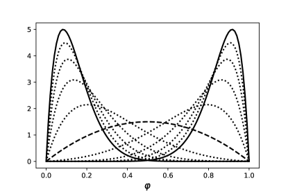
Figure 2: Updated density functions for $\varphi$, each computed under the model $\varphi\sim\mathrm{Beta}(2,2)$, $\theta_{j}\sim\mathrm{Bernoulli}(\varphi)$, $j=1,\ldots,10$, with soft observations $\Pi_{j}(\theta_{j}=k)$, $k\in\{0,1\}$, assumed to be identical for all $j$. The different densities are obtained by varying $\Pi_{j}(\theta_{j}=1)$ from 0 to 1 by increments of 0.1. The solid curves correspond to $\Pi_{j}(\theta_{j}=1)=0$ and $\Pi_{j}(\theta_{j}=1)=1$, equivalent to posteriors computed conditional on all $\theta_{j}$ fully observed with values 0 and 1, respectively. The dashed curve corresponds to $\Pi_{j}(\theta_{j}=1)=0.5$, and equals the prior $\mathrm{Beta}(2,2)$. For further details, see Example 1 .

2.1 Theoretical properties

Two well-known properties of standard Bayesian inference, which are of practical relevance in our meta-analysis setting, are (i) order-invariance in successive posterior updates of exchangeable models and (ii) posterior concentration. The former ensures that inferences conditional on exchangeable data are coherent. The latter tells us that the posterior distribution becomes increasingly informative about the quantity of interest, as we accumulate more data. We will now briefly discuss these properties in the context of the framework introduced above.

2.1.1 Order-invariance in successive posterior updates

Under the assumption of exchangeability, standard Bayesian inference can be constructed as a sequence of successive updates, invariant to the order in which the data are processed. The following proposition establishes that the update rule defined in Equation (5) retains the same property.

Proposition 2.1.

The update rule defined in Equation (5) is invariant to permutations of the indices $1,\ldots,J$.

Proof.

It suffices for us to verify the claim for $J=2$. Beginning with $J=1$, we update the probability $Q(B)$ into $Q^{*}(B|\Pi_{1})$ using Equation (5):

$$Q^{*}(B|\Pi_{1})=\frac{\int_{B}\int_{\Theta}p(\theta_{1}|\varphi)\Pi_{1}(d\theta_{1})Q(d\varphi)}{\int_{\Phi}\int_{\Theta}p(\theta_{1}|\varphi)\Pi_{1}(d\theta_{1})Q(d\varphi)}.$$

Then, we reapply Equation (5) to update $Q^{*}(B|\Pi_{1})$ into $Q^{*}(B|\Pi_{1},\Pi_{2})$:

$$Q^{*}(B|\Pi_{1},\Pi_{2}) =\frac{\int_{B}\int_{\Theta}p(\theta_{2}|\varphi)\Pi_{2}(d\theta_{2})Q^{*}(d\varphi|\Pi_{1})}{\int_{\Phi}\int_{\Theta}p(\theta_{2}|\varphi)\Pi_{2}(d\theta_{2})Q^{*}(d\varphi|\Pi_{1})}$$

$$=\frac{\int_{B}\int_{\Theta}p(\theta_{2}|\varphi)\Pi_{2}(d\theta_{2})}{\int_{\Phi}\int_{\Theta}p(\theta_{2}|\varphi)\Pi_{2}(d\theta_{2})}\frac{\frac{\int_{\Theta}p(\theta_{1}|\varphi)\Pi_{1}(d\theta_{1})Q(d\varphi)}{\cancel{\int_{\Phi}\int_{\Theta}p(\theta_{1}|\varphi)\Pi_{1}(d\theta_{1})Q(d\varphi)}}}{\frac{\int_{\Theta}p(\theta_{1}|\varphi)\Pi_{1}(d\theta_{1})Q(d\varphi)}{\cancel{\int_{\Phi}\int_{\Theta}p(\theta_{1}|\varphi)\Pi_{1}(d\theta_{1})Q(d\varphi)}}}$$

$$=\frac{\int_{B}\prod_{j=1}^{2}\left[\int_{\Theta}p(\theta_{j}|\varphi)\Pi_{j}(d\theta_{j})\right]Q(d\varphi)}{\int_{\Phi}\prod_{j=1}^{2}\left[\int_{\Theta}p(\theta_{j}|\varphi)\Pi_{j}(d\theta_{j})\right]Q(d\varphi)},$$

which is equivalent to a direct application of Equation (5) for $J=2$, and independent of the order in which $\Pi_{1}$ and $\Pi_{2}$ are processed. ∎

As an alternative strategy to Equation (5), we could first attempt to formulate a posterior distribution $Q(\cdot|\theta_{1},\ldots,\theta_{J})$ according to Equation (4) and then, as a final step, integrate out the uncertainty in the conditioning set with respect to the observed beliefs. This is in essence the strategy of Jeffrey’s rule of conditioning. It is, however, well known that Jeffrey’s update rule is in general not order-invariant (Diaconis and Zabell, 1982).

2.1.2 Posterior concentration

Asymptotic theory states that if a consistent estimator of the true value (or an optimal one in terms KL-divergence) of the parameter $\varphi$ exists, then the posterior distribution (4) concentrates in a neighborhood of this value, as $J\rightarrow\infty$ (e.g. Schervish, 1995). Here we discuss conditions under which the same property holds for the measure $Q^{*}(\cdot|\Pi_{1},\ldots,\Pi_{J})$, defined in Equation (5). Considerations of asymptotic normality will not be discussed here.

Our strategy is to first formulate a generative hierarchical model for the observed distributions $\Pi_{1},\ldots,\Pi_{J}$. Then, we show that $Q^{*}(\cdot|\Pi_{1},\ldots,\Pi_{J})$ can be expressed as the marginal posterior distribution of $\varphi$ in this model. Finally, we show that under some further technical conditions, standard asymptotic theory can be applied to this distribution. To this end, consider the following hierarchical model:

$$\varphi \sim Q$$ (7a)

$$\theta_{j} \sim P_{\varphi}$$ (7b)

$$\Pi_{j} \sim G^{(j)}_{\theta_{j}},$$ (7c)

where $\Pi_{j}$ is treated as a soft observation of the unobserved value of $\theta_{j}$, and $G^{(j)}_{\theta_{j}}$ is the inference mechanism that produces $\Pi_{j}$. Note that in the particular case of $\Pi_{j}$ being the Dirac measure, $G^{(j)}_{\theta_{j}}$ simply generates a point mass at the true value of $\theta_{j}$, such that the hierarchical model reduces to an ordinary, non-hierarchical Bayesian model. Since $\Pi_{j}$ is an inference over the values of $\theta_{j}$, produced by $G^{(j)}_{\theta_{j}}$, it is also a direct representation of the likelihood of $\theta_{j}$ under the model $G^{(j)}_{\theta_{j}}$, given the observation $\Pi_{j}$ itself. We finally note, that the generating mechanism $G^{(j)}_{\theta_{j}}$ may in general be different for each $j$, which is highlighted in the notation by the superscript.

Assume now that the Radon-Nikodym derivative $g_{j}(\cdot|\theta_{j}):=dG^{(j)}_{\theta_{j}}/d\kappa$ with respect to a dominating measure $\kappa\gg G^{(j)}_{\theta_{j}}$ can be defined for all $j$. The marginal posterior distribution of $\varphi$ is then

$$Q^{\prime}(B|\Pi_{1},\ldots,\Pi_{J})=\frac{\int_{B}\prod_{j=1}^{J}\left[\int_{\Theta}g_{j}(\Pi_{j}|\theta_{j})P_{\varphi}(d\theta_{j})\right]Q(d\varphi)}{\int_{\Phi}\prod_{j=1}^{J}\left[\int_{\Theta}g_{j}(\Pi_{j}|\theta_{j})P_{\varphi}(d\theta_{j})\right]Q(d\varphi)},$$

where $g_{j}(\Pi_{j}|\theta_{j})$, taken as a function of $\theta_{j}$, is the likelihood of $\theta_{j}$ given $\Pi_{j}$. On the other hand, according to our previous assumption, the likelihood is directly encapsulated in $\Pi_{j}$ itself. We will therefore assume, by construction, that $g_{j}(\Pi_{j}|\theta_{j})=\pi_{j}(\theta_{j})$, where $\pi_{j}:=d\Pi_{j}/d\lambda$ is the density function corresponding to $\Pi_{j}$. Using this equivalence, we state the following lemma:

Lemma 2.2.

Let $g_{j}(\Pi_{j}|\theta_{j})=\pi_{j}(\theta_{j})$. Then the measures $Q^{\prime}(\cdot|\Pi_{1},\ldots,\Pi_{J})$ and $Q^{*}(\cdot|\Pi_{1},\ldots,\Pi_{J})$ are equivalent.

Proof.

To prove the claim, we only need to verify that the integrals $\int_{\Theta}g_{j}(\Pi_{j}|\theta_{j})P_{\varphi}(d\theta_{j})$ and $\int_{\Theta}p_{j}(\theta_{j}|\varphi)\Pi_{j}(d\theta_{j})$ are equivalent. Since $\Pi_{j}$ and $P_{\varphi}$ are both probability distributions on $(\Theta,\mathcal{A})$, and their densities are defined with respect to the same reference measure $\lambda$, we may swap the roles of the integrand and the measure that we integrate against:

$$\int_{\Theta}g_{j}(\Pi_{j}|\theta_{j})P_{\varphi}(d\theta_{j}) =\int_{\Theta}\pi_{j}(\theta_{j})P_{\varphi}(d\theta_{j})$$

$$=\int_{\Theta}\frac{d}{d\lambda}\Pi_{j}(\theta_{j})P_{\varphi}(d\theta_{j})$$

$$=\int_{\Theta}\frac{d}{d\lambda}P_{\varphi}(\theta_{j})\Pi_{j}(d\theta_{j})$$

$$=\int_{\Theta}p_{j}(\theta_{j}|\varphi)\Pi_{j}(d\theta_{j}).$$

∎

Corollary 2.2.1.

In the hierarchical model (7a)–(7c), let $H^{(j)}_{\varphi}$ be the marginal conditional distribution of $\Pi_{j}$, given $\varphi$, and let $h_{j}(\Pi_{j}|\varphi):=\int_{\Theta}g_{j}(\Pi_{j}|\theta_{j})P_{\varphi}(d\theta_{j})$ be the corresponding marginal likelihood. Following Lemma 2.2, the probability $Q^{*}(B|\Pi_{1},\ldots,\Pi_{J})$ can be written as

$$Q^{*}(B|\Pi_{1},\ldots,\Pi_{J})=\frac{\int_{B}\prod_{j=1}^{J}h_{j}(\Pi_{j}|\varphi)Q(d\varphi)}{\int_{\Phi}\prod_{j=1}^{J}h_{j}(\Pi_{j}|\varphi)Q(d\varphi)}.$$

The essential difference between the standard posterior distribution defined in Equation (4) and that of Corollary 2.2.1 above, is that in the former, the observations are conditionally i.i.d., while in the latter they are conditionally independent but non-identically distributed.

Assuming that there exists, for all $j$, a unique minimizer $\varphi_{0}$ of the KL-divergence from the true distribution of $\Pi_{j}$ to the parametrized representation $H_{\varphi}^{(j)}$, a key step in proving posterior concentration is to establish a limit for the log-likelihood ratio $\sum_{j=1}^{J}\log\frac{h_{j}(\Pi_{j}|\varphi)}{h_{j}(\Pi_{j}|\varphi_{0})}$. Since the summands are now non-identically distributed, standard forms of the strong law of large numbers cannot be applied to obtain this limit. However, with further conditions imposed on the second moment of each term in the sum, an alternative form can be used, which relaxes the requirement of the terms being identically distributed (Sen and Singer, 1993, Theorem 2.3.10). The conditions are stated in the following theorem.

Theorem 2.3.

Assume that the log-likelihood ratio terms $\xi_{j}:=\log\frac{h_{j}(\Pi_{j}|\varphi)}{h_{j}(\Pi_{j}|\varphi_{0})}$ are independent, and that $\mathds{E}(\xi_{j})=\mu_{j}$ and $\mathrm{Var}(\xi_{j})=\sigma_{j}^{2}$ exist for all $j\geq 1$. Let $\overline{\mu}_{J}=J^{-1}\sum_{j=1}^{J}\mu_{j}$, for $J\geq 1$. Then

$$\sum_{j\geq 1}j^{-2}\sigma_{j}^{2}<\infty\Rightarrow J^{-1}\sum_{j=1}^{J}\xi_{j}-\overline{\mu}_{J}\xrightarrow{\text{a.s.}}0.$$

In conclusion, if the measure $Q^{*}(\cdot|\Pi_{1},\ldots,\Pi_{J})$ can be written in the form of Equation (2.2.1) and the conditions of Theorem 2.3 hold, then posterior concentration falls back to the standard case, for which elementary proofs can be found in many sources (e.g. Bernardo and Smith, 1994; Gelman et al., 2013). A rigorous treatment is given in Schervish (1995). As an example, we provide a proof of posterior concentration of $Q^{*}(\cdot|\Pi_{1},\ldots,\Pi_{J})$ for discrete parameter spaces in Appendix A.

3 Meta-analysis of Bayesian analyses

We now turn to a practical view of the framework developed in the previous section. To this end, it is convenient to work with densities instead of measures. We are motivated by the problem of conducting meta-analysis for Bayesian analyses summarized as posterior distributions, and refer to our framework as meta-analysis of Bayesian analyses (MBA). The central belief updates of the framework are given in Equations (9) and (10), which update beliefs regarding global and local effects, respectively. Figures 3(a) and 3(b) visualize the updates by interpreting them as message passing in probabilistic graphical models.

To reiterate the setting laid out in Section 1, we assume that a set of posterior density functions $\{\pi_{1},\ldots,\pi_{J}\}$ is available, each expressing a belief about the value of a corresponding quantity of interest in a set $\{\theta_{1},\ldots,\theta_{J}\}$. While the density functions can be thought of as resulting from previously conducted Bayesian analyses, it is worth pointing out that from a methodological point of view, we are agnostic to how they have been formed; instead of posteriors, some (or all) of the $\pi_{j}$’s could be purely subjective prior beliefs, or as discussed in Section 2, even directly observed values.

Judging the quantities $\theta_{j}$ to be exchangeable, the meta-analyst now formulates a model

$$\prod_{j=1}^{J}p(\theta_{j}|\varphi)q(\varphi),$$ (8)

with an appropriate prior $q$ placed on the parameter $\varphi$. Note that this model initially makes no reference to the $\pi_{j}$’s, and it is formulated as if the $\theta_{j}$’s were fully observable quantities. Then, to update $q$ based on the observed density functions, we apply Equation (5) in density form to have

$$q^{*}(\varphi)\propto\prod_{j=1}^{J}\left[\int_{\Theta}p(\theta_{j}|\varphi)\pi_{j}(\theta_{j})d\theta_{j}\right]q(\varphi),$$ (9)

where for brevity, we denote $q^{*}:=q^{*}(\cdot|\Pi_{1},\ldots,\Pi_{J})$.

In a meta-analysis context, the parameter $\varphi$ often has an interpretation as the central tendency of some shared property of $\theta_{1},\ldots,\theta_{J}$, such as the mean or the covariance (or both jointly). As such, inference on $\varphi$ is often of primary interest in providing a ‘consensus’ over a number of studies. As a secondary goal, we may also be interested in updating a (possibly weakly informative) belief about any individual quantity $\theta_{j}$, subject to the information provided by observations on the remaining quantities. To do so, we first write Equation (6) in density form:

$$p^{*}(\theta_{1},\ldots,\theta_{J})\propto\int_{\Phi}\prod_{j=1}^{J}\left[p(\theta_{j}|\varphi)\pi_{j}(\theta_{j})d\theta_{j}\right]q(\varphi)d\varphi,$$

and then marginalize over all quantities but the one to be updated. Let $\mathcal{J}:=\{1,\ldots,J\}$ be a set of indices and let $j^{\prime}\in\mathcal{J}$ be an arbitrary index in this set. The density function $\pi_{j^{\prime}}$ is then updated as follows:

$$\pi_{j^{\prime}}^{*}(\theta_{j^{\prime}})\propto\int_{\Phi}p(\theta_{j^{\prime}}|\varphi)\pi_{j^{\prime}}(\theta_{j^{\prime}})\prod_{j\in\mathcal{J}\setminus j^{\prime}}^{J}\left[\int_{\Theta}p(\theta_{j}|\varphi)\pi_{j}(\theta_{j})d\theta_{j}\right]q(\varphi)d\varphi.$$ (10)

Remark 1.

According to Section 2.1.2, the density $q^{*}(\varphi)$, defined in Equation (9), will under suitable conditions become increasingly peaked around some point $\varphi_{0}$, as $J\rightarrow\infty$. That $\pi_{j^{\prime}}^{*}(\theta_{j})$ does not behave similarly, becomes clear by the following considerations. First, we note that Equation (10) is equivalent to

$$\pi_{j^{\prime}}^{*}(\theta_{j^{\prime}})=Z_{j^{\prime}}^{-1}\pi_{j^{\prime}}(\theta_{j^{\prime}})\int_{\Phi}p(\theta_{j^{\prime}}|\varphi)q^{*}(\varphi|\Pi_{1},\ldots,\Pi_{j^{\prime}-1},\Pi_{j^{\prime}+1},\ldots,\Pi_{J})\,d\varphi,$$

where $Z_{j}$ is a normalizing constant. As $q^{*}(\varphi|\Pi_{1},\ldots,\Pi_{j^{\prime}-1},\Pi_{j^{\prime}+1},\ldots,\Pi_{J})$ becomes increasingly peaked around $\varphi_{0}$, the integral in the above equation converges to $p(\theta_{j^{\prime}}|\varphi_{0})$. Consequently,

$$\pi_{j^{\prime}}^{*}(\theta_{j^{\prime}})\rightarrow Z_{j^{\prime}}^{-1}\pi_{j^{\prime}}(\theta_{j^{\prime}})p(\theta_{j^{\prime}}|\varphi_{0}),$$

which can only be degenerate if either $\pi_{j^{\prime}}(\theta_{j^{\prime}})$ or $p(\theta_{j^{\prime}}|\varphi_{0})$ is degenerate by design. Instead of degeneracy, $\pi_{j^{\prime}}^{*}(\theta_{j^{\prime}})$ exhibits shrinkage with respect to $\varphi_{0}$.

3.1 Interpretation as message passing

The formulation of the above meta-analysis framework, constructed as an extension of standard Bayesian inference, can also be viewed within the formalism of probabilistic graphical models. This provides both an intuitive interpretation and a visualization of Equations (9) and (10), and gives a straightforward way of extending the framework to more complex model structures. To elaborate further on this, consider a tree-structured undirected graphical model with $J$ leaf nodes and a root. This is a special case of a pairwise Markov random network (Koller and Friedman, 2009), where all factors, or clique potentials, are over single variables or pairs of variables, referred to as node and edge potentials, respectively. Note that the potential functions are simply non-negative functions, which may not integrate to 1. Choosing, for $j=1,\ldots,J$, the node potentials as $\pi_{j}(\theta_{j})$ and $q(\varphi)$, and the edge potentials as $\psi_{j}(\theta_{j},\varphi):=p(\theta_{j}|\varphi)$, the model has the joint density

$$\frac{1}{Z}q(\varphi)\prod_{j=1}^{J}\psi_{j}(\theta_{j},\varphi)\pi_{j}(\theta_{j}),$$

where $Z$ is a normalizing constant. Finding the marginal density of $\varphi$ can then be interpreted as propagating beliefs from each of the leaf nodes up to the root node in the form of messages, a process known as message passing or belief propagation (e.g. Yedidia et al., 2001). To that end, we specify the following messages to be sent from the $j$th leaf node to the root:

$$m_{\theta_{j}\rightarrow\varphi}(\varphi)\propto\int\psi_{j}(\theta_{j},\varphi)\pi_{j}(\theta_{j})d\theta_{j}.$$ (11)

The initial belief $q(\varphi)$ on $\varphi$ is then updated according to

$$q^{*}(\varphi)\propto q(\varphi)\prod_{j=1}^{J}m_{\theta_{j}\rightarrow\varphi}(\varphi),$$ (12)

which is exactly equal to Equation (9), and illustrated in Figure 3(a).

In a similar way, we may pass information to any single leaf node from the remaining leaf nodes. We now specify two kinds of messages: from leaf nodes indexed by $j\in\mathcal{J}\setminus j^{\prime}$ to the root node, as given by Equation (11), and from the root node to the $j^{\prime}$th leaf node,

$$m_{\varphi\rightarrow\theta_{j^{\prime}}}(\theta_{j^{\prime}})\propto\int_{\Phi}\psi_{j^{\prime}}(\varphi,\theta_{j^{\prime}})q(\varphi)\prod_{j\in\mathcal{J}\setminus j^{\prime}}m_{\theta_{j}\rightarrow\varphi}(\varphi)\,d\varphi.$$

The updated belief over $\theta_{j^{\prime}}$ is then

$$\pi_{j^{\prime}}^{*}(\theta_{j^{\prime}})\propto\pi_{j^{\prime}}(\theta_{j^{\prime}})m_{\varphi\rightarrow\theta_{j^{\prime}}}(\theta_{j^{\prime}}),$$ (13)

which is exactly equal to Equation (10), and illustrated in Figure 3(b).

(a)  

(b)  

Figure 3: Propagating beliefs by messages-passing (a) from each of the leaf nodes to the root node and (b) from each of the nodes $\theta_{2},\ldots,\theta_{J}$ to $\varphi$, and then finally, from $\varphi$ to $\theta_{1}$. The updated beliefs over $\varphi$ and $\theta_{1}$ are $q^{*}(\varphi)\propto q(\varphi)\prod_{j=1}^{J}m_{\theta_{j}\rightarrow\varphi}(\varphi)$ and $\pi_{1}^{*}(\theta_{1})\propto\pi_{1}(\theta_{1})\,m_{\varphi\rightarrow\theta_{1}}(\theta_{1})$, respectively.

Although not directly utilized in this work, the graphical model view may also be useful in devising efficient computational strategies (see also the remarks in Section 7). Especially with more complex model structures, making use of the conditional independencies made explicit by the graphical model may bring considerable computational gains.

3.2 Bayesian meta-analysis as a special case

It is straightforward to show that Bayesian random-effects and fixed-effects meta-analyses can be recovered as special cases of the proposed framework. In its traditional formulation (e.g. Normand, 1999), random-effects meta-analysis (REMA) assumes that for each of $J$ studies, a summary statistic, $D_{j}$, $j=1,\ldots,J$, has been observed, drawn from a distribution with study-specific mean $\mathds{E}(D_{j})=\theta_{j}$ and variance $\mathrm{Var}(D_{j})=\sigma_{j}^{2}$:

$$D_{j}\sim\mathcal{N}(\theta_{j},\sigma_{j}^{2}),$$ (14)

where the approximation of the distribution of $D_{j}$ by a normal distribution is justified by the asymptotic normality of maximum likelihood estimates. The variances $\sigma_{j}^{2}$ are directly estimated from the data, while the means $\theta_{j}$, are assumed to be drawn from some common distribution, typically

$$\theta_{j}\sim\mathcal{N}(\mu,\sigma_{0}^{2}),$$

where the parameters $\mu$ and $\sigma_{0}^{2}$ represent the average treatment effect and inter-study variation, respectively. Fixed-effects meta-analysis is a special case of REMA, where $\sigma_{0}^{2}=0$, such that $\theta_{1}=\theta_{2}=\cdots=\theta_{J}$.

The posterior density for the parameters $(\mu,\sigma_{0}^{2})$ in REMA can be written as

$$q(\mu,\sigma_{0}^{2}|D_{1},\ldots,D_{J}) \propto q(\mu,\sigma_{0}^{2})\prod_{j=1}^{J}\int_{\Theta}N(D_{j}|\theta_{j},\hat{\sigma}_{j}^{2})N(\theta_{j}|\mu,\sigma_{0}^{2})d\theta_{j}$$

$$\propto q(\mu,\sigma_{0}^{2})\prod_{j=1}^{J}\int_{\Theta}l(\theta_{j};D_{j})N(\theta_{j}|\mu,\sigma_{0}^{2})d\theta_{j},$$

where $N(\cdot|\cdot,\cdot)$ denotes a Gaussian density function, $l(\theta_{j};D_{j})$ is the likelihood function of $\theta_{j}$ given $D_{j}$, and $\hat{\sigma}_{j}^{2}$ is the empirical variance of $D_{j}$. To study the connection between the above posterior density and Equation (9), assume that instead of a summary statistic $D_{j}$, each study has been summarized using a posterior distribution with density $\pi_{j}(\theta_{j})$ over its study-specific effect parameter $\theta_{j}$. If the distribution has been computed under the data model given by equation (14), and using an improper uniform prior $\nu_{j}(\theta_{j})\propto 1$, the density is

$$\pi_{j}(\theta_{j})=N(\theta_{j}|D_{j},\hat{\sigma}_{j}^{2})\propto\exp\left\{-\frac{(D_{j}-\theta_{j})^{2}}{2\hat{\sigma}_{j}^{2}}\right\}=l(\theta_{j};D_{j}),$$

resulting in the posterior density of $(\mu,\sigma_{0}^{2})$ being equivalent in both cases.

4 Computation

Here we describe a simple computational strategy, which is used in the numerical examples of Section 5 below. Some further alternatives are briefly discussed at the end of this section. Recall now that the density of the joint distribution of the parameters $\theta_{1},\ldots,\theta_{J},\varphi$ can be written as

$$\frac{1}{Z}q(\varphi)\prod_{j=1}^{J}p_{j}(\theta_{j}|\varphi)\pi_{j}(\theta_{j}).$$ (15)

Our goal is to produce joint samples from the above model, enabling any desired marginals to be extracted from them. Probabilistic programming languages (e.g. Carpenter et al., 2017; Salvatier et al., 2015; Tran et al., 2016; Wood et al., 2014) allow sampling from an arbitrary model, provided that the components of the (unnormalized) model can be specified in terms of probability distributions of some standard form. In the illustrations of this section, we use Hamiltonian Monte Carlo implemented in the Stan probabilistic programming language (Carpenter et al., 2017).

We first note that in the above joint model (15), the part specified by the meta-analyst, i.e. $q(\varphi)\prod_{j=1}^{J}p_{j}(\theta_{j}|\varphi)$, can by design be composed using standard parametric distributions. The observed part of the model $\prod_{j=1}^{J}\pi_{j}(\theta_{j})$, however, is in general analytically intractable, and instead of having direct access to posterior density functions of standard parametric form, we typically have a sets of posterior samples $\left\{\theta_{j}^{(1)},\ldots,\theta_{j}^{(L_{j})}\right\}$, with $\theta_{j}^{(l)}\sim\Pi_{j}$. Our strategy is then to first find an intermediate parametric approximation $\hat{\pi}_{j}$ for $\pi_{j}$, which enables us to sample from an approximate joint distribution. Assuming that the true densities $\pi_{j}(\theta_{j})$ can be evaluated using e.g. kernel density estimation, and that $\hat{\pi}_{j}(\theta_{j})=0\Rightarrow\pi_{j}(\theta_{j})=0$, the joint samples can be further refined using sampling/importance resampling (SIR; Smith and Gelfand, 1992). The steps of the computational scheme are summarized below:

1. For $j=1,\ldots,J$, fit a parametric density function $\hat{\pi}_{j}$ to the samples $\left\{\theta_{j}^{(1)},\ldots,\theta_{j}^{(L_{j})}\right\}$.

2. Draw $M$ samples $\mathcal{S}=\left\{\theta_{1}^{*\,(m)},\ldots,\theta_{J}^{*\,(m)},\varphi^{*\,(m)}\right\}_{m=1}^{M}$ from the approximate joint model $\frac{1}{Z^{\prime}}q(\varphi)\prod_{j=1}^{J}\psi_{j}(\theta_{j},\varphi)\hat{\pi}_{j}(\theta_{j})$.

3. Compute importance weights $w_{m}=\tilde{w}_{m}/\sum_{m=1}^{M}\tilde{w}_{m}$, where

   $$\tilde{w}_{m} =\frac{Z^{-1}\,q\left(\varphi^{*\,(m)}\right)\prod_{j=1}^{J}\psi_{j}\left(\theta_{j}^{*\,(m)},\varphi^{*\,(m)}\right)\pi_{j}\left(\theta_{j}^{*\,(m)}\right)}{(Z^{\prime})^{-1}\,q\left(\varphi^{*\,(m)}\right)\prod_{j=1}^{J}\psi_{j}\left(\theta_{j}^{*\,(m)},\varphi^{*\,(m)}\right)\hat{\pi}_{j}\left(\theta_{j}^{*\,(m)}\right)}$$

   $$=\frac{Z^{\prime}\,\prod_{j=1}^{J}\pi_{j}\left(\theta_{j}^{*\,(m)}\right)}{Z\,\prod_{j=1}^{J}\hat{\pi}_{j}\left(\theta_{j}^{*\,(m)}\right)}.$$

   Note that the constant $Z^{\prime}/Z$ cancels in the computation of the normalized weights $w_{m}$.

4. Resample $\mathcal{S}$ with weights $\{w_{1},\ldots,w_{M}\}$.

For problems with a very large number of studies or high dimensional local parameters, or if the imposed parametric densities approximate the actual posteriors poorly, the computation of importance weights may become numerically unstable. The issue could possibly be mitigated using more advanced importance sampling schemes, such as Pareto-smoothed importance sampling (Vehtari et al., 2015) or prior swap importance sampling (Neiswanger and Xing, 2017). If we are only interested in sampling from the density of the global parameter, as given by Equation (9), then an obvious alternative strategy would be to implement a Metropolis-Hastings algorithm, using the samples $\theta_{j}^{(l)}\sim\Pi_{j}$ to compute Monte Carlo estimates of the integrals $\int_{\Theta}p(\theta_{j}|\varphi)\pi_{j}(\theta_{j})d\theta_{j}$. However, this would lead to expensive MCMC updates as the integrals need to be re-estimated at every iteration of the algorithm. Finally, instead of directly sampling from the full joint distribution, we could try to utilize the induced graphical model structure (Section 3.1) to do localized inference, see also Section 7.

5 Numerical illustrations

In this section, we illustrate our meta-analysis framework, meta-analysis of Bayesian analyses (MBA), with numerical examples. In these examples, we consider the problem of combining results from analyses conducted using likelihood-free models. In such models, the data can typically be summarized by a number of different statistics but there is no closed-form likelihood to relate these to the quantity or effect of interest, which poses a challenge for traditional formulations of meta-analysis. In our framework, we directly utilize the inferred posteriors to build a joint model. In addition to modeling the shared central tendency of the inferred model parameters, we demonstrate that weakly informative or poorly identifiable posteriors for individual studies can be updated post-hoc through joint modeling. We begin with a brief review of likelihood-free inference using approximate Bayesian computation.

5.1 Likelihood-free inference using approximate Bayesian computation

Approximate Bayesian computation (ABC) is a paradigm for Bayesian inference in models, which either entirely lack an analytically tractable likelihood function, or for which it is costly to compute. The only requirement is that we are able to sample data from the model by fixing values for the parameters of interest, as is the case for simulator-based models. In the basic form of ABC, simulations are run for parameter proposals drawn from a prior distribution. The parameter proposals whose simulated data $x_{\theta}$ match the observed data $x_{0}$ are collected and constitute a sample from the posterior distribution. It can be shown that this process is equivalent to accepting parameter proposals in proportion to their likelihood value, given the observed data, as is done in traditional rejection sampling.

In practice, the simulated data virtually never exactly matches the observed data and likely no sample from the posterior distribution would be acquired. This problem can be circumvented by loosening the acceptance condition to accept samples whose simulations yield results similar enough to the observed data. For this purpose, a dissimilarity function $d$ and a scalar $\varepsilon>0$ are defined such that a parameter proposal with respective simulation result $x_{\theta}$ is accepted if $d(x_{\theta},x_{0})\leq\varepsilon$. This function is often defined in terms of summary statistics $s(x_{\theta})$ and $s(x_{0})$. For example, $d$ could be defined as the Euclidean distance between $s(x_{\theta})$ and $s(x_{0})$. The aforementioned relaxation results in samples being drawn from an approximate posterior instead of the actual posterior distribution, hence the name approximate Bayesian computation.

For a comprehensive introduction to ABC, see Marin et al. (2012). More recent developments are reviewed in Lintusaari et al. (2017). In the following numerical illustrations, posterior distributions obtained using ABC provide a starting point for meta-analysis. These likelihood-free inferences are implemented using the ELFI open-source software package (Lintusaari et al., 2018).

5.2 Example 1: MA$(q)$ process

In our first example, we use simulated data from a MA$(q)$ process of order $q=2$. The MA$(q)$ process is a standard example in the literature on likelihood-free inference due to its simple structure but fairly complex likelihood and non-trivial relationship between parameters and observed data. Assuming zero mean, the process $(y_{t})_{t\in\mathbb{N}^{+}}$ is defined as

$$y_{t}=\epsilon_{t}+\theta_{1}\epsilon_{t-1}+\theta_{2}\epsilon_{t-2},$$ (16)

where $(\theta_{1},\theta_{2})\in\mathbb{R}^{2}$ and $\epsilon_{s}\sim\mathcal{N}(0,1)$, ${s\in\mathbb{Z}}$. The quantity of interest for which we conduct inference is $\boldsymbol{\theta}=(\theta_{1},\theta_{2})$. Following Marin et al. (2012), we use as prior for $\boldsymbol{\theta}$ a uniform distribution over the set

$$\mathcal{T}\subset\mathbb{R}^{2}\triangleq\{(\theta_{1},\theta_{2})\in\mathbb{R}^{2}|-(\theta_{2}+1)<\theta_{1}<\theta_{2}+1,\;-1<\theta_{2}<1\},$$

which, by restriction of the parameter space, imposes a general identifiability condition for MA$(q)$ processes. Inference for $\boldsymbol{\theta}$ is then conducted using ABC with rejection sampling, taking as summary statistics the empirical autocovariances of lags one and two, denoted as $\hat{\gamma}_{1}$ and $\hat{\gamma}_{2}$, respectively. Furthermore, a Euclidean distance of 0.1 is used as acceptance threshold.

To illustrate our meta-analysis framework, we first sample $J=12$ realizations of $\boldsymbol{\theta}$ using the following generating process:

$$\theta_{1}\sim\mathrm{Unif}(0.4,0.8),\quad\theta_{2}\sim\mathcal{N}(-0.4+\theta_{1j},0.04^{2}).$$ (17)

Given each realization $\boldsymbol{\theta}_{j}=(\theta_{1j},\theta_{2j})$, $j=1,\ldots,J$, we then generate a series of $10$ data points, $(y_{j1},\ldots,y_{j10})$, according to Equation (16). For each time-series, we independently conduct likelihood-free inference as described above, generating $1000$ samples from the posterior. The computed posterior distributions along with their corresponding true parameter values are shown in Figure 4. It can be seen that the very limited information given by the data in each of the analyses leaves the posteriors with a considerable amount of uncertainty.

For meta-analysis, we first specify a model for the study-specific effects $\boldsymbol{\theta}_{1},\ldots,\boldsymbol{\theta}_{J}$ as if they were observed quantities from an exchangeable sequence; see Equation (8). As the true generating mechanism of the effects is typically unknown, the model must be specified according to the analyst’s judgment. To reflect this, we will here model the generating process as a Gaussian distribution with parameters $\varphi=(\boldsymbol{\mu},\Sigma_{0})$,

$$\boldsymbol{\theta}_{j}\sim\mathcal{N}_{2}(\boldsymbol{\mu},\Sigma_{0}).$$ (18)

For $\boldsymbol{\mu}$ and the covariance matrix $\Sigma_{0}$, we use Gaussian and inverse Wishart priors, respectively,

$$\centering\boldsymbol{\mu}\sim\mathcal{N}_{2}(\boldsymbol{m},V)\quad\text{ and }\quad\Sigma_{0}\sim\mathcal{W}^{-1}(\nu,\Psi)\,,\@add@centering$$ (19)

with

$$\centering\boldsymbol{m}=\begin{bmatrix}1/2\\ 0\end{bmatrix},\quad V=\begin{bmatrix}0.4&0.05\\ 0.05&0.1\end{bmatrix},\quad\text{ and }\quad\nu=4,\quad\Psi=\begin{bmatrix}0.4&0.1\\ 0.1&0.2\end{bmatrix}.\@add@centering$$

The above values were chosen to provide reasonable coverage of $\mathcal{T}$, the constrained support of $\boldsymbol{\theta}$. Furthermore, $\nu$ was chosen as $\mathrm{dim}(\boldsymbol{\theta})+2$ to directly yield $\Psi$ as the mean of the inverse Wishart prior on $\Sigma_{0}$.

After specifying the assumed generative model for $\boldsymbol{\theta}_{1},\ldots,\boldsymbol{\theta}_{J}$ according to Equations (18)–(19), the following step is to incorporate the observed beliefs for each $\boldsymbol{\theta}_{j}$ into the inference. For computational convenience, we initially approximate the study-specific posteriors using a suitable parametric family. In our current example, we fit a bivariate normal distribution to each of the $J=12$ posteriors. Following the computational scheme presented in Section 4, inference for the joint model was carried out using Hamiltonian Monte Carlo implemented in the Stan software (Carpenter et al., 2017), and finally, the results were refined using SIR.

We compare MBA against results obtained using traditional random-effects meta-analysis (REMA), as specified in Section 3.2. The likelihood of REMA is given by the model

$$\hat{\!\boldsymbol{\theta}}_{j}\sim\mathcal{N}_{2}(\boldsymbol{\theta}_{j},\hat{\Sigma}_{j}),$$ (20)

wwhere the effect estimates $\,\hat{\!\boldsymbol{\theta}}_{j}=(\hat{\theta}_{1j},\hat{\theta}_{2j})$ are computed numerically using conditional sum of squares and the study-specific covariance matrices $\hat{\Sigma}_{j}$ are estimated using bootstrap. The hierarchical distribution on $\boldsymbol{\theta}_{j}$ follows Equations (18) and (19) above. Therefore, the essential difference between REMA and MBA is whether we combine this distribution with a likelihood function based on Equation (20) or with the observed posterior on $\boldsymbol{\theta}_{j}$. The results of the comparison are presented in Figures 5–7.

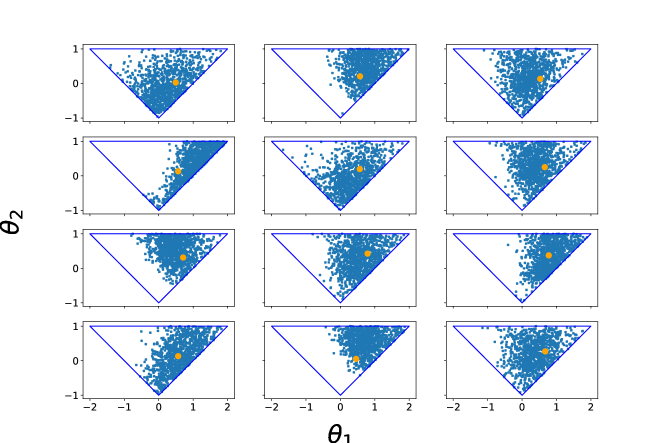
Figure 4: Posterior samples for the parameters $(\theta_{1j},\theta_{2j})$ of $J=12$ MA$(2)$ processes, obtained using rejection-sampling ABC. The yellow dots denote the true generating parameter values.

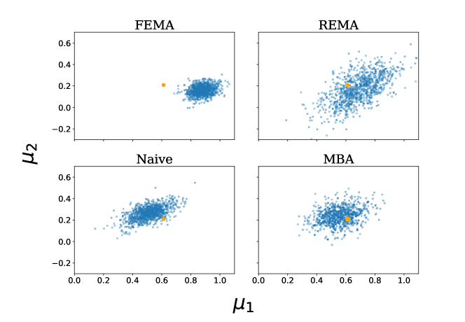
Figure 5: Posterior for the global mean effect $\boldsymbol{\mu}$ using FEMA, REMA, a ‘naive’ model, and MBA. The yellow dot denotes the actual mean of the distribution used to generate the $\boldsymbol{\theta}_{j}$ values for the MA(2) series.

Figure 6: Updated posteriors for the the study-specific effects obtained using MBA (red) on top of the ones originally obtained using independent ABC’s (blue). The yellow dots denote the true generating parameter values.

Figure 7: Posterior marginals for the study-specific effects obtained using REMA (red) on top of the posteriors originally obtained using independent ABC’s (blue). The yellow dots denote the true generating parameter values.

Figure 5 shows the posterior distribution for the global mean effect $\boldsymbol{\mu}$, obtained using four different models: in addition to MBA and REMA, we used fixed-effects meta-analysis (FEMA, which is a special case of REMA, see Section 3.2), and a ’naive’ model corresponding to ordinary Bayesian inference using the means of the observed posteriors on $\boldsymbol{\theta}_{j}$ as observed data. As expected, FEMA is clearly inappropriate in this situation, and results in a heavily biased and overly confident posterior. The naive model is less biased than FEMA as it makes use of information contained in the observed posteriors, but compared to MBA, it does not properly account for the uncertainty contained in them. Both REMA and MBA result in posteriors with more spread, still assigning reasonably high probability mass to the neighbourhood around the true parameter value. Figure 6 shows updated beliefs for the local effects, obtained using the update rule of Equation (10) in Section 3, also schematically depicted in Figure 3(b). The updated beliefs exhibit shrinkage towards the global mean effect and, in this case, concentrate more accurately around the actual local effect values. On the other hand, many of the REMA posteriors for the local effects, shown in Figure 7, are biased and concentrate in regions away from true values.

5.3 Example 2: Tuberculosis outbreak dynamics

We now apply MBA to conduct meta-analysis of parameters regulating a stochastic birth-death (SBD) model proposed by Lintusaari et al. (2019), who used their model in a single-study setting to analyze tuberculosis outbreak data from the San Francisco Bay area, initially reported by Small et al. (1994). The goal of the analysis was to estimate disease transmission parameters from genotype data which, in contrast to outbreak models relying on count data,renders the likelihood-function intractable and necessitates the use of likelihood-free inference (Tanaka et al., 2006). Furthermore, such models are often complex in relation to the available data, which may result in poor identifiability, as discussed by Lintusaari et al. (2016). To alleviate the problem, they formulated their model as a mixture of stochastic processes, taking into account the individual transmission dynamics of different subpopulations. In our analyses, we focus on two key parameters of the model, $R_{1}$ and $R_{2}$, which are the reproductive numbers for two subpopulations: those that are compliant and non-compliant to treatment, respectively.

For our current experiment, we analyzed three additional data sets using the model of Lintusaari et al. (2019). These data sets reported tuberculosis outbreaks in Estonia (Krüüner et al., 2001), London (Maguire et al., 2002) and the Netherlands (van Soolingen et al., 1999). For each data set, we independently conducted likelihood-free inference, generating $1000$ samples from the posteriors. Following Lintusaari et al. (2019), we used the following six summary statistics for the ABC simulations: the number of observations, the total number of genotype clusters, the size of the largest cluster, the proportion of clusters of size two, the proportion of singleton clusters, and finally, the average successive difference in size among the four largest clusters. The original publication additionally used two summary statistics on the observation times of the largest cluster. While these were found to improve model identifiability, such information was not available for the additional data sets analyzed in our current experiment. We used a weighted Euclidean distance as dissimilarity function, with the same weights as in Lintusaari et al. (2019).

Figure 8 shows the joint posterior distributions for the parameters $R_{1}$ and $R_{2}$, obtained individually for all four geographical locations using ABC. Compared to the San Francisco data, the posteriors computed on the remaining data sets, in particular London and the Netherlands, show severe problems with identifiability. This can at least partly be attributed to these data sets being less informative than the San Francisco data set. A key question for our experiment then is whether we could borrow strength across the studies to improve the identifiability of the models computed on the remaining data sets. Additionally, it will be of interest to obtain an overall analysis of the central tendency of the reproductive numbers.

As in the previous experiment of Section 5.2, we first define a model for the local effects $\boldsymbol{\theta}_{j}=(R_{1j},R_{2j})$, and assign priors for the global mean effect $\boldsymbol{\mu}=(\mu_{1},\mu_{2})$ and the covariance matrix $\Sigma_{0}$, resulting in the model:

$$\boldsymbol{\theta}_{j}\sim\mathcal{N}_{2}(\boldsymbol{\mu},\Sigma_{0}),$$

$$\mu_{1}\sim\mathrm{Gamma}(a_{1},b_{1}),$$

$$\mu_{2}\sim\mathrm{Gamma}(a_{2},b_{2}),$$

$$\Sigma_{0}\sim\mathcal{W}^{-1}(\nu,\Psi).$$

The hyper-parameters were set as follows:

$$a_{1}=0.12,\,b_{1}=0.36\quad a_{2}=.030,\,b_{2}=0.05,\quad\text{ and }\quad\nu=4,\quad\Psi=\begin{bmatrix}4&-0.1\\ -0.1&0.01\end{bmatrix}.$$

We then incorporate the observed beliefs by fitting a bivariate Gaussian distribution to each of the $J=4$ study-specific ABC posteriors. Inference is performed using Stan and the obtained posterior is improved using SIR. Note that due to the indirect nature in the relationship between the infection data and the parameters of interest, using the data to directly construct an estimator for the parameters of interest would be difficult. While this does not pose a challenge in our framework, it renders the application of traditional meta-analysis approaches infeasible.

Figure 9 shows the updated beliefs for the local effects $\boldsymbol{\theta}_{1},\ldots,\boldsymbol{\theta}_{J}$, after borrowing strength across the individual studies. While the updated beliefs clearly retain some of the individual characteristics of their original counterparts (e.g. a similar covariance structure), they exhibit a much more identifiable behavior. The posterior of the overall mean of the reproductive numbers is shown in Figure 10.

Figure 8: Posteriors for the reproductive numbers $(R_{1},R_{2})$, individually obtained using ABC in four different studies on tuberculosis outbreak dynamics.

Figure 9: Posteriors for the reproductive numbers $(R_{1},R_{2})$ updated using MBA (red), plotted on top of the original, individually obtained posteriors (blue).

Figure 10: MBA joint posterior for the overall mean effect $\boldsymbol{\mu}=(\mu_{1},\mu_{2})$.

6 Related work

To the best of our knowledge, meta-analysis frameworks for combining posterior distributions have not been presented before. Nonetheless, similar elements can be found in a number of previous works. Xie et al. (2011) proposed to do meta-analysis by combining confidence distributions which, despite their analogy with Bayesian posterior marginals, is a concept deeply rooted in the frequentist paradigm, see Schweder and Hjort (2002). In the context of Bayesian meta-analysis, Lunn et al. (2013) introduced a two-stage computational approach for fitting hierarchical models to individual-level data. In the first stage, posterior samples for local parameters are generated independently for each study, enabling study-specific complexities to be dealt with separately. In a second stage, the samples are used as proposals in Metropolis-Hastings updates within a Gibbs algorithm to fit the full hierarchical model. While the paper focuses on a specific computational approach for hierarchical models, involving no propagation of local prior knowledge into the joint model, the idea of utilizing independently computed posterior samples to fit a joint model is common to our framework.

In recent work, Rodrigues et al. (2016) developed a hierarchical Gaussian process prior to model a set of related density functions, where grouped data in the form of samples assumed to be drawn under each density function are available. Despite a superficial similarity between their work and ours, the inferential goals in these works are very different. Specifically, the former is concerned with nonparametric estimation of group-specific densities, which is shown to be useful when the sample sizes in some or all of the groups are small. Thus, in cases where the number of posterior samples per study is limited (e.g. due to computational reasons), the method of Rodrigues et al. (2016) could be used within our framework to provide density estimates for the initial beliefs.

7 Conclusion

The natural outcome of a Bayesian analysis is a posterior distribution over quantities of interest. In this paper, we have developed a framework which, instead of study-specific data summaries or individual-level data, uses estimated posterior distributions to conduct meta-analysis. The framework builds on standard Bayesian inference over exchangeable observations, by treating each observed posterior as data observed with uncertainty.

In Section 3.1, we showed that the proposed framework can be interpreted as message passing in probabilistic graphical models. Utilizing this interpretation, a graphical illustration of the main update formulas, Equations (9) and (10), is given in Figure 3(a) and 3(b), respectively. In future work, we plan to further investigate computational strategies which make use of this interpretation. Unlike our current strategy, which infers all parameters of the joint model simultaneously, utilization of localized inference would enable us to devise more efficient and flexible computational schemes. In particular, recent developments in nonparametric and particle-based belief propagation (Ihler and McAllester, 2009; Lienart et al., 2015; Pacheco et al., 2014; Sudderth et al., 2010) represent a promising direction in this line of work.

In many fields, it has become common practice to store data sets in dedicated repositories to be reused for the benefit of the entire research community. Given the view taken in this work, that posterior distributions can be seen as a special kind of observational data, we believe that in many cases it would be equally beneficial to make full posterior distributions available for reuse. This would enable posteriors from potentially time-consuming and costly Bayesian analyses to be used as a basis for new studies. Indeed, even if the original data, the model and the code implementing it were available, reproducing posterior distributions could require a substantial computational effort. In addition to making posteriors publicly available, more research is needed on developing methods to make appropriate use of the information they provide. The current work is a first step in this direction and our hope is that it will inspire other researchers to make further advances to this end.

Appendix A Posterior concentration for discrete parameters

Here, we give an elementary proof of posterior concentration of $Q(\cdot|\Pi_{1},\ldots,\Pi_{J})$ for discrete parameter spaces. The proof follows the basic structure found in many sources (e.g. Bernardo and Smith, 1994; Gelman et al., 2013), with the essential difference that the observations are independent but non-identically distributed.

Theorem A.1.

Let $\{\Pi_{1},\ldots,\Pi_{J}\}$ be a set of observations from a corresponding set of distributions $\{R_{1},\ldots,R_{J}\}$. Furthermore, let $\left\{\{H^{(j)}_{\varphi}|\varphi\in\Phi\}\right\}_{j=1}^{J}$ be a set of families, such that

• $\Phi$ consists of (at most) a countable set of values,

• $\varphi_{0}=\operatorname*{arg\,min}_{\varphi\in\Phi}\mathrm{KL}\left(R_{j}||H^{(j)}_{\varphi}\right)$, for all $j$.

If the conditions of Theorem 2.3 hold, and furthermore if $\sum_{\varphi\in\Phi}Q(\varphi)=1$ and $Q(\varphi_{0})>0$, then $Q^{*}(\varphi_{0}|\Pi_{1}\ldots,\Pi_{J})\rightarrow 1$, as $J\rightarrow\infty$.

Proof.

For any $\varphi\neq\varphi_{0}$, the log posterior odds can written as

$$\log\frac{Q\left(\varphi|\Pi_{1},\ldots,\Pi_{J}\right)}{Q\left(\varphi_{0}|\Pi_{1},\ldots,\Pi_{J}\right)}=\log\frac{Q(\varphi)}{Q(\varphi_{0})}+\sum_{j=1}^{J}\log\frac{h_{j}(\Pi_{j}|\varphi)}{h_{j}(\Pi_{j}|\varphi_{0})},$$ (21)

where the second term is a sum of $J$ independent but non-identically distributed random variables. By Theorem 2.3, we have that

$$\frac{1}{J}\sum_{j=1}^{J}\log\frac{h_{j}(\Pi_{j}|\varphi)}{h_{j}(\Pi_{j}|\varphi_{0})}\rightarrow\mathds{E}\left(\log\frac{h_{j}(\Pi_{j}|\varphi)}{h_{j}(\Pi_{j}|\varphi_{0})}\right),$$

with probability 1, as $J\rightarrow\infty$. Since $\varphi_{0}$ is the unique minimizer of the KL-divergence $\mathrm{KL}\left(R_{j}||H^{(j)}_{\varphi}\right)$, by definition

$$\mathds{E}\left(\log\frac{h_{j}(\Pi_{j}|\varphi)}{h_{j}(\Pi_{j}|\varphi_{0})}\right)=\mathrm{KL}\left(R^{j}||H^{j}_{\varphi_{0}}\right)-\mathrm{KL}\left(R^{j}||H^{j}_{\varphi}\right)<0,$$

and consequently,

$$\sum_{j=1}^{J}\log\frac{h_{j}(\Pi_{j}|\varphi)}{h_{j}(\Pi_{j}|\varphi_{0})}\rightarrow-\infty.$$

Since $Q(\varphi_{0})>0$, the entire expression (21) approaches $-\infty$ as $J\rightarrow\infty$, which implies that $Q(\varphi|\Pi_{1},\ldots,\Pi_{J})\rightarrow 0$ and $Q(\varphi_{0}|\Pi_{1},\ldots,\Pi_{J})\rightarrow 1$. ∎

References

- Albert et al. (2012) Albert, I., S. Donnet, C. Guihenneuc-Jouyaux, S. Low-Choy, K. Mengersen, and J. Rousseau (2012). Combining expert opinions in prior elicitation. Bayesian Anal. 7(3), 503–532.
- Bernardo and Smith (1994) Bernardo, J. M. and A. F. M. Smith (1994). Bayesian Theory. Chichester: John Wiley & Sons, Inc.
- Carpenter et al. (2017) Carpenter, B., A. Gelman, M. Hoffman, D. Lee, B. Goodrich, M. Betancourt, M. Brubaker, J. Guo, P. Li, and A. Riddell (2017). Stan: A probabilistic programming language. J. Statist. Soft. 76(1).
- Diaconis and Zabell (1982) Diaconis, P. and S. L. Zabell (1982). Updating subjective probability. J. Am. Statist. Ass. 77(380), 822–830.
- Gelman et al. (2013) Gelman, A., J. Carlin, H. Stern, D. Dunson, A. Vehtari, and D. Rubin (2013). Bayesian Data Analysis, Third Edition (Chapman & Hall/CRC Texts in Statistical Science) (Third ed.). London: Chapman and Hall/CRC.
- Higgins et al. (2009) Higgins, P. T., S. G. Thompson, and D. J. Spiegelhalter (2009). A re-evaluation of random-effects meta-analysis. J. R. Statist. Soc. A 172(1), 137–159.
- Ihler and McAllester (2009) Ihler, A. and D. McAllester (2009). Particle belief propagation. In Proc. 12nd Int. Conf. Artificial Intelligence and Statistics., Volume 5, pp. 256–263.
- Jeffrey (2004) Jeffrey, R. (2004). Subjective Probability: The Real Thing. New York: Cambridge University Press.
- Jordan (2004) Jordan, M. I. (2004, 02). Graphical models. Statist. Sci. 19(1), 140–155.
- Koller and Friedman (2009) Koller, D. and N. Friedman (2009). Probabilistic Graphical Models: Principles and Techniques. The MIT Press.
- Krüüner et al. (2001) Krüüner, A., S. E. Hoffner, H. Sillastu, M. Danilovits, K. Levina, S. B. Svenson, S. Ghebremichael, T. Koivula, and G. Källenius (2001). Spread of drug-resistant pulmonary tuberculosis in estonia. J. of Clincl Microb. 39(9), 3339–3345.
- Kuikka et al. (2014) Kuikka, S., J. Vanhatalo, H. Pulkkinen, S. Mäntyniemi, and J. Corander (2014). Experiences in Bayesian inference in Baltic salmon management. Statist. Sci. 29(1), 42–49.
- Lienart et al. (2015) Lienart, T., Y. W. Teh, and A. Doucet (2015). Expectation particle belief propagation. In Advances in Neural Information Processing Systems 28, pp. 3609–3617. Curran Associates, Inc.
- Lintusaari et al. (2019) Lintusaari, J., P. Blomstedt, T. Sivula, M. Gutmann, S. Kaski, and J. Corander (2019). Resolving outbreak dynamics using approximate Bayesian computation for stochastic birth-death models [version 1; referees: awaiting peer review]. Wellcome Open Research 4(14).
- Lintusaari et al. (2017) Lintusaari, J., M. U. Gutmann, R. Dutta, S. Kaski, and J. Corander (2017). Fundamentals and recent developments in approximate Bayesian computation. System. Biol. 66(1), e66–e82.
- Lintusaari et al. (2016) Lintusaari, J., M. U. Gutmann, S. Kaski, and J. Corander (2016). On the identifiability of transmission dynamic models for infectious diseases. Genetics 202(3), 911–918.
- Lintusaari et al. (2018) Lintusaari, J., H. Vuollekoski, A. Kangasrääsiö, K. Skytén, M. Järvenpää, P. Marttinen, M. U. Gutmann, A. Vehtari, J. Corander, and S. Kaski (2018). ELFI: Engine for likelihood-free inference. J. Mach. Learn. Res. 19(16), 1–7.
- Lunn et al. (2013) Lunn, D., J. Barrett, M. Sweeting, and S. Thompson (2013). Fully Bayesian hierarchical modelling in two stages, with application to meta-analysis. J. R. Statist. Soc. C 62(4), 551–572.
- Maguire et al. (2002) Maguire, H., J. W. Dale, T. D. McHugh, P. D. Butcher, S. H. Gillespie, A. Costetsos, H. Al-Ghusein, R. Holland, A. Dickens, L. Marston, P. Wilson, R. Pitman, D. Strachan, F. A. Drobniewski, and D. K. Banerjee (2002). Molecular epidemiology of tuberculosis in london 1995–7 showing low rate of active transmission. Thorax 57(7), 617–622.
- Marin et al. (2012) Marin, J.-M., P. Pudlo, C. P. Robert, and R. J. Ryder (2012). Approximate Bayesian computational methods. Statist. Comp. 22(6), 1167–1180.
- Neiswanger and Xing (2017) Neiswanger, W. and E. Xing (2017). Post-inference prior swapping. In Proc. 34th Int. Conf. Machine Learning, Volume 70, pp. 2594–2602.
- Normand (1999) Normand, S.-L. T. (1999). Meta-analysis: formulating, evaluating, combining, and reporting. Statist. Medcn 18, 321–359.
- Pacheco et al. (2014) Pacheco, J., S. Zuffi, M. Black, and E. Sudderth (2014, 22–24 Jun). Preserving modes and messages via diverse particle selection. In Proc. 31st Int. Conf. Machine Learning, Volume 32, pp. 1152–1160.
- Rodrigues et al. (2016) Rodrigues, G., D. J. Nott, and S. Sisson (2016). Functional regression approximate Bayesian computation for Gaussian process density estimation. Computnl Statist. Data Anal. 103, 229–241.
- Salvatier et al. (2015) Salvatier, J., T. Wiecki, and C. Fonnesbeck (2015). Probabilistic programming in python using PyMC. Preprint arXiv:1507.08050.
- Schervish (1995) Schervish, M. J. (1995). Theory of statistics. New York: Springer.
- Schweder and Hjort (2002) Schweder, T. and N. L. Hjort (2002). Confidence and likelihood. Scand. J. Statist. 29(2), 309–332.
- Sen and Singer (1993) Sen, P. K. and J. M. Singer (1993). Large Sample Methods in Statistics: An Introduction with Applications. Boca Raton: Chapman & Hall/CRC.
- Small et al. (1994) Small, P. M., P. C. Hopewell, S. P. Singh, A. Paz, J. Parsonnet, D. C. Ruston, G. F. Schecter, C. L. Daley, and G. K. Schoolnik (1994). The epidemiology of tuberculosis in San Francisco – a population-based study using conventional and molecular methods. New Eng. J. Med. 330(24), 1703–1709.
- Smets (1993) Smets, P. (1993). Jeffrey’s rule of conditioning generalized to belief functions. In Proc. 9th Conf. Uncertainty in Artificial Intelligence (UAI-93), pp. 500–505.
- Smith and Gelfand (1992) Smith, A. F. M. and A. E. Gelfand (1992). Bayesian statistics without tears: A sampling–resampling perspective. The American Statistician 46(2), 84–88.
- Sudderth et al. (2010) Sudderth, E. B., A. T. Ihler, M. Isard, W. T. Freeman, and A. S. Willsky (2010, October). Nonparametric belief propagation. Commun. ACM 53(10), 95–103.
- Tanaka et al. (2006) Tanaka, M. M., A. R. Francis, F. Luciani, and S. A. Sisson (2006). Using approximate Bayesian computation to estimate tuberculosis transmission parameters from genotype data. Genetics 173(3), 1511–1520.
- Tran et al. (2016) Tran, D., A. Kucukelbir, A. B. Dieng, M. Rudolph, D. Liang, and D. M. Blei (2016). Edward: A library for probabilistic modeling, inference, and criticism. Preprint arXiv:1610.09787.
- van Soolingen et al. (1999) van Soolingen, D., M. W. Borgdorff, P. E. W. de Haas, M. M. G. G. Sebek, J. Veen, M. Dessens, K. Kremer, and J. D. A. van Embden (1999). Molecular epidemiology of tuberculosis in the netherlands: A nationwide study from 1993 through 1997. J Infect. Dis. 180(3), 726–736.
- Vehtari et al. (2015) Vehtari, A., A. Gelman, and J. Gabry (2015). Pareto smoothed importance sampling. Preprint arXiv:1507.02646.
- Wood et al. (2014) Wood, F., J. W. Meent, and V. Mansinghka (2014). A New Approach to Probabilistic Programming Inference. In Proc. 17th Int. Conf. Artificial Intelligence and Statistics, Volume 33, pp. 1024–1032.
- Xie et al. (2011) Xie, M., K. Singh, and W. E. Strawderman (2011). Confidence distributions and a unifying framework for meta-analysis. J. Am. Statist. Ass. 106(493), 320–333.
- Yedidia et al. (2001) Yedidia, J. S., W. T. Freeman, and Y. Weiss (2001). Generalized belief propagation. In Advances in Neural Information Processing Systems 13, pp. 689–695. MIT Press.
- Zhao and Osherson (2010) Zhao, J. and D. Osherson (2010). Updating beliefs in light of uncertain evidence: Descriptive assessment of Jeffrey’s rule. Thinking & Reasoning 16(4), 288–307.