Kernelized Complete Conditional Stein Discrepancies

Abstract

Much of machine learning relies on comparing distributions with discrepancy measures. Stein’s method creates discrepancy measures between two distributions that require only the unnormalized density of one and samples from the other. Stein discrepancies can be combined with kernels to define kernelized Stein discrepancies (ksds). While kernels make Stein discrepancies tractable, they pose several challenges in high dimensions. We introduce kernelized complete conditional Stein discrepancies (kcc-sds). Complete conditionals turn a multivariate distribution into multiple univariate distributions. We show that kcc-sds distinguish distributions. To show the efficacy of kcc-sds in distinguishing distributions, we introduce a goodness-of-fit test using kcc-sds. We empirically show that kcc-sds have higher power over baselines and use kcc-sds to assess sample quality in Markov chain Monte Carlo.

1 Introduction

Discrepancy measures that compare a distribution $p$, known up to normalization, with a distribution $q$, known via samples from it, can be used for finding good variational approximations (Ranganath et al., 2016; Liu and Wang, 2016), checking the quality of mcmc samplers (Gorham and Mackey, 2015, 2017), goodness-of-fit testing (Liu et al., 2016), parameter estimation (Barp et al., 2019) and multiple model comparison (Lim et al., 2019). There are several difficulties with using traditional discrepancies like Wasserstein metrics or total variation distance for these tasks. Mainly, $p$ can be hard to sample so expectations under $p$ cannot be computed. These challenges lead to the following desiderata for a discrepancy $D$ (Gorham and Mackey, 2015).

1. Tractable $D$ uses samples from $q$, and evaluations of (unnormalized) $p$.

2. Distinguishing Distributions $D(p,q)=0$ if and only if $p$ is equal in distribution to $q$.

These desiderata ensure that the discrepancy is non zero when $p$ does not equal $q$ and that it can be easily computed. To meet these desiderata, Chwialkowski et al. (2016); Oates et al. (2017); Gorham and Mackey (2017); Liu et al. (2016) developed kernelized Stein discrepancies (ksds). ksds measure the expectation of functions under $q$ that have expectation zero under $p$. These functions are constructed by applying Stein’s operator to a reproducing kernel Hilbert space (rkhs).

In high dimensions, many popular kernels evaluated on a pair of points are near zero. Thus, ksds in high dimensions can be near zero, making detecting differences between high dimensional distributions difficult. The median heuristic can be used to address this to some extent, but ksds with the median heuristic can still have low power in moderately high dimensions (see Figure 1, Jitkrittum et al. (2017)). We develop kernelized complete conditional Stein discrepancies (kcc-sds). These discrepancies use complete conditionals: the distribution of one variable given the rest. Complete conditionals are univariate distributions. Rather than using multivariate kernels, kcc-sds use univariate kernels to ensure the complete conditionals match, making it easier to compare distributions in high dimensions.

A given Stein discrepancy relies on a supremum over a class of test functions called the Stein set. kcc-sds differ from ksds in that kcc-sds compute a separate supremum for each complete conditional. An immediate question is whether there is a computable closed form and whether the discrepancy can be used to distinguish distributions. We show that kcc-sds have a closed form and distinguish between distributions. Computing kcc-sd requires sampling from a complete conditional of $q$, which can be infeasible in some instances. To address this, we introduce approximate kcc-sd that uses a learned sampler for the complete conditional.

To show the efficacy of kcc-sd and approximate kcc-sd in distinguishing distributions we introduce a goodness-of-fit test (Chwialkowski et al., 2016). We show that kcc-sd and approximate kcc-sd have higher power than ksd and other baselines. We empirically show that approximate kcc-sd does not suffer from a loss in power due to an increase in dimension. We also demonstrate that kcc-sd and approximate kcc-sd can be used to select sampler hyperparameters and can be used to assess sample quality in a Gibbs sampler.

Related Work.

There have been several lines of work which use factorizations of the distribution $p$ to address the curse of dimensionality. Wang et al. (2017); Zhuo et al. (2017) use the Markov blanket of each node to define a graphical version of ksd to alleviate the curse of dimensionality. Our approach does not presume a graphical structure of $p$ or $q$. Wang et al. (2017) shows that unless the graphical structure for $p,q_{n}$ match, the graph based ksd converging to zero does not imply that $q_{n}$ converges in distribution to $p$.

Gong et al. (2020) introduce the maximum sliced kernelized Stein discrepancy (MAXsksd), which also uses low-dimensional kernels by projecting into a $1$-dimensional space. Computing MAXsksd requires optimizing a projection direction that is specific to both sampling distribution $q$ and the unnormalized distribution $p$. This can be expensive when testing multiple distributions or when changing the parameters of an unnormalized model to fit a collection of samples. Approximate kcc-sd requires learning conditional distributions specific only to the sampling distribution $q$. Similar to approximate kcc-sd with parametric conditional estimates, the closed form for MAXsksd depends on the optimal direction, therefore the power of their method depends on the quality of the optimization, which can be difficult to guarantee for arbitrary log probabilities.

ksds suffer from a computational cost that is quadratic in the number of samples. Huggins and Mackey (2018) develop random feature Stein discrepancies r$\Phi$sd, which run in linear time and perform as well as or better than quadratic-time ksds; these ideas can be applied to kcc-sds. Chen et al. (2018) introduces the Stein points method which introduces a method to select points to minimize the Stein discrepancy between the empirical distribution supported at the selected points and the posterior.

Chwialkowski et al. (2016) introduced ksd as a test statistic for a goodness-of-fit test, which also suffers from the curse of dimensionality due to the use of kernels in high dimensions, along with a computational cost quadratic in the number of samples. Jitkrittum et al. (2017) introduce a linear-time discrepancy, finite-set Stein discrepancy (fssd). The authors introduce an optimized version of fssd which allows one to find features that best indicate the differences between the samples and the target density. fssd while having a computational cost linear in sample size, also leads to a test with lower power in high dimensions.

2 Kernelized Stein Discrepancies

Stein’s method provides recipes for constructing expectation zero test functions of distributions known up to a normalization constant. For a distribution $p$ with a integrable score function, $\nabla_{\bm{x}}\log p(\bm{x})$, we can create a Stein operator, $\mathcal{A}_{p}$, that acts on test functions $f:\mathbb{R}^{d}\rightarrow\mathbb{R}^{d}$ satisfying regularity and boundary conditions (Proposition 1, (Gorham and Mackey, 2015)), such that

$$\mathbb{E}_{p(\bm{x})}\left[\mathcal{A}_{p(\bm{x})}f(\bm{x})\right]=0.$$

This relation called Stein’s identity is used to create Stein discrepancies $\mathcal{S}(q,\mathcal{A}_{p},\mathcal{H})$, defined as

$$\mathcal{S}(q,\mathcal{A}_{p},\mathcal{H}) =\sup_{f\in\mathcal{H}}\left|\mathbb{E}_{q(\bm{x})}[\mathcal{A}_{p(\bm{x})}f(\bm{x})]-\mathbb{E}_{p(\bm{x})}[\mathcal{A}_{p(\bm{x})}f(\bm{x})]\right|$$

$$=\sup_{f\in\mathcal{H}}\left|\mathbb{E}_{q(\bm{x})}\left[\mathcal{A}_{p(\bm{x})}f(\bm{x})\right]\right|\ ,$$

where $\mathcal{H}$ is a function space known as the Stein set, with its functions satisfying some boundary and regularity conditions. To make the Stein discrepancy simpler to compute, Chwialkowski et al. (2016); Oates et al. (2017); Gorham and Mackey (2017); Liu et al. (2016) used reproducing kernel Hilbert spaces (rkhs) as the Stein set to introduce kernelized Stein discrepancies (ksd). Let $k:\mathbb{R}^{d}\times\mathbb{R}^{d}\rightarrow\mathbb{R}$ be the kernel of an rkhs $\mathcal{K}_{k}$, the rkhs consists of functions, $g:\mathbb{R}^{d}\rightarrow\mathbb{R}$, satisfying the reproducing property $g(\bm{x})={\langle{g,k(\bm{x},\cdot)}\rangle}_{\mathcal{K}_{k}}$. ksds are defined by the Stein set

$$\mathcal{G}_{k}=\left\{g=(g_{1},\dots,g_{d}):g_{i}\in\mathcal{K}_{k},\sum_{i=1}^{d}\left\lVert g_{i}\right\rVert_{\mathcal{K}_{k}}\leq 1\right\}\ .$$

This construction of the Stein set using an rkhs ensures that the Stein discrepancy has a closed form.

Proposition 1 (Gorham and Mackey, 2017).

Suppose $k\in C^{(1,1)}$ and for each $j\in\{1,\dots,d\}$, define the Stein kernel as follows:

$$k_{0}^{j}(\bm{x},\bm{y}) =b_{j}(\bm{x})b_{j}(\bm{y})k(\bm{x},\bm{y})+\nabla_{x_{j}}\nabla_{y_{j}}k(\bm{x},\bm{y})$$ (1)

$$\quad+b_{j}(\bm{x})\nabla_{y_{j}}k(\bm{x},\bm{y})+b_{j}(\bm{y})\nabla_{x_{j}}k(\bm{x},\bm{y})\ ,$$

where $b_{j}(\bm{x})=\nabla_{x_{j}}\log p(\bm{x})$. If $\sum_{j=1}^{d}\mathbb{E}_{q}[{k_{0}^{j}(\bm{x},\bm{x})}^{1/2}]<\infty$, then ksd has a closed form. Given by $\mathcal{S}(q,\mathcal{A}_{p},\mathcal{G}_{k})=\left\lVert\bm{w}\right\rVert_{2}$, where $w_{j}^{2}\equiv\mathbb{E}_{q(\bm{x})\times q(\bm{y})}\left[k_{0}^{j}(\bm{x},\bm{y})\right]$ with $\bm{x},\bm{y}\overset{i.i.d}{\sim}q$.

When the distribution $p$ lies in the class of distantly dissipative distributions (Eberle, 2016), ksds provably detect convergence and non-convergence for $d=1$. That is $\mathcal{S}(q_{n},\mathcal{A}_{p},\mathcal{G}_{k})\rightarrow 0$ if and only if $q_{n}\Rightarrow p$ for sequences $\{q_{n}\}$, using kernels like the radial basis function or the inverse multi-quadratic (imq), (Gorham and Mackey, 2017). In $d>2$, the ksd with thin tailed kernels like the rbf does not detect non-convergence. But the ksd with the imq kernel with $\beta\in(0,1)$ does detect non-convergence. However, all of these kernels shrink as the $\left\lVert\cdot\right\rVert_{2}$ grows, which means their associated ksds become less sensitive in higher dimensions.

Suppose $\bm{x},\bm{y}\sim N(\bm{0},I_{d})$ then $\mathbb{E}[\left\lVert\bm{x}-\bm{y}\right\rVert^{2}]=2d$, so $k(\bm{x},\bm{y})=\exp(-\left\lVert\bm{x}-\bm{y}\right\rVert^{2}/2\sigma^{2})$ concentrates around $\exp(-d/\sigma^{2})$. The median heuristic, $\sigma=\text{median}({\left\lVert\bm{x}_{i}-\bm{x}_{j}\right\rVert;i<j})$, can be used to deal with this shrinkage. However, (Ramdas et al., 2015) show that even with the median heuristic, kernel based discrepancies can converge to zero as the dimension increases even when the distributions are different.

3 Kernelized Complete Conditional Stein Discrepancies.

Complete conditionals are univariate conditional distributions, $p(x_{j}|\bm{x}_{-j})$, where $\bm{x}_{-j}=\{x_{1},\dots x_{j-1},x_{j+1},\dots x_{d}\}$. Complete conditional distributions are the basis for many inference procedures including the Gibbs sampler (Geman and Geman, 1984), and coordinate ascent variational inference (Ghahramani and Beal, 2001).

Using complete conditionals we construct complete conditional Stein discrepancies (cc-sds) and their kernelized versions (kcc-sds). In this work we focus on the Langevin-Stein operator (Barbour, 1990; Gorham and Mackey, 2015), defined for differentiable functions $f:\mathbb{R}^{d}\rightarrow\mathbb{R}^{d}$ as follows:

$$(\mathcal{A}_{p(\bm{x})}f)(\bm{x})={f(\bm{x})}^{T}\nabla_{\bm{x}}\log p(\bm{x})+\nabla_{\bm{x}}\cdot f(\bm{x})=\sum_{j=1}^{d}\mathcal{A}^{j}_{p(\bm{x})}f_{j}(\bm{x})\ .$$

Definition.

The score function of the complete conditional, $\nabla_{x_{j}}\log p(x_{j}\mid\bm{x}_{-j})$, is the score function of the joint, $\nabla_{x_{j}}\log p(\bm{x})$. So for $f_{j}:\mathbb{R}^{d}\rightarrow\mathbb{R}$,

$$\mathcal{A}^{j}_{p(x_{j}\mid\bm{x}_{-j})}f_{j}(\bm{x}) =f_{j}(\bm{x})\nabla_{x_{j}}\log p(x_{j}\mid\bm{x}_{-j})+\nabla_{x_{j}}f_{j}(\bm{x})=f_{j}(\bm{x})\nabla_{x_{j}}\log p(\bm{x})+\nabla_{x_{j}}f_{j}(\bm{x})$$

$$=\mathcal{A}_{p(\bm{x})}^{j}f_{j}(\bm{x})$$

Using this observation, and the fact that the complete conditionals of two distributions $p,q$ match when the distributions match, we define the complete conditional Stein discrepancy (cc-sd), $\mathcal{S}(q,\mathcal{A}_{p},\mathcal{C})$ as

$$\sum_{j=1}^{d}\mathbb{E}_{q(\bm{x}_{-j})}\left[\sup_{f_{j}\in\mathcal{C}^{j}}\mathbb{E}_{q(x_{j}\mid\bm{x}_{-j})}[\mathcal{A}^{j}_{p(x_{j}\mid\bm{x}_{-j})}f_{j}(\bm{x})]\right]\ .$$ (2)

The Stein set $\mathcal{C}$ is defined as the set of functions, $f:\mathbb{R}^{d}\rightarrow\mathbb{R}^{d}$, with each component $f_{j}(\bm{x})$ satisfying $\max\left(\left\lVert f_{j}\right\rVert_{\infty},\left\lVert\nabla f_{j}\right\rVert_{\infty},Lip(f_{j})\right)\leq 1$, where $Lip(f)$ is the Lipschitz constant of $f$. Here, the supremum is taken inside the expectation, so we have to solve optimization problems for each dimension and each conditional. Similar to Stein discrepancies, cc-sds can be hard to compute. In the next section, we introduce the kernelized version which has a closed form.

3.1 Kernelized Complete Conditional Stein Discrepancies.

We now define the Stein set, $\mathcal{C}_{k}$, for the kernelized version of cc-sd, such that we get a closed form discrepancy.

We use univariate integrally symmetric positive definite (ispd) kernels, $k:\mathbb{R}\times\mathbb{R}\rightarrow\mathbb{R}$, that satisfy the following, for $g:\mathbb{R}\rightarrow\mathbb{R}$:

$$\int_{u\in\mathbb{R}}\int_{v\in\mathbb{R}}g(u)k(u,v)g(v)dudv>0\ ,$$ (3)

with $\left\lVert g\right\rVert_{2}>0$. Let $\mathcal{K}_{k}$ denote the reproducing kernel Hilbert space (rkhs) with kernel $k$. Functions $h\in\mathcal{K}_{k}$ satisfy the reproducing property, $h(x_{j})=\langle{h,k(x_{j},\cdot)}\rangle_{\mathcal{K}_{k}}$ for $x_{j}\in\mathbb{R}$. The rkhs also satisfies $\Phi_{x_{j}}(\cdot)=k(x_{j},\cdot)\in\mathcal{K}_{k}$.

We define $\mathcal{C}_{k}$ with a univariate kernel $k$, as consisting of functions, $f:\mathbb{R}^{d}\rightarrow\mathbb{R}^{d}$, whose component functions $f_{j}:\mathbb{R}^{d}\rightarrow\mathbb{R}$ satisfy $f_{j,\bm{x}_{-j}}\equiv f_{j}(\cdot,\bm{x}_{-j})\in\mathcal{K}_{k}$ for each $\bm{x}_{-j}$. So $f_{j}$ with a fixed $\bm{x}_{-j}$ is in the rkhs defined by $k$. This means

$$f_{j,\bm{x}_{-j}}(x_{j})=\langle{f_{j,\bm{x}_{-j}},k(x_{j},\cdot)}\rangle_{\mathcal{K}_{k}}\ .$$ (4)

Let $\mathcal{C}_{k}^{j}$ denote the set of functions satisfying Equation 4 with norm bounded by

$$\left\lVert f_{j,\bm{x}_{-j}}\right\rVert_{\mathcal{K}_{k}}\leq\left\lVert\mathbb{E}_{q(x_{j}\mid\bm{x}_{-j})}\left[\mathcal{A}^{j}_{p(x_{j}\mid\bm{x}_{-j})}\Phi_{x_{j}}\right]\right\rVert_{\mathcal{K}_{k}}\ ,$$ (5)

for all $\bm{x}_{-j}\in\mathbb{R}^{d-1}$.

We define the kernelized complete conditional Stein discrepancy (kcc-sd) $\mathcal{S}(q,\mathcal{A}_{p},\mathcal{C}_{k})$ as follows,

$$\sum_{j=1}^{d}\mathbb{E}_{q(\bm{x}_{-j})}\left[\left|\sup_{f_{j}\in\mathcal{C}_{k}^{j}}\mathbb{E}_{q(x_{j}\mid\bm{x}_{-j})}\left[\mathcal{A}^{j}_{p(x_{j}\mid\bm{x}_{-j})}f_{j}(\bm{x})\right]\right|\right]$$ (6)

KCC-SDs admit a closed form.

In our definition of the Stein set, we can change the kernel or the kernel parameters in each dimension, however for clarity we do not focus on that here. Note that the Stein set depends on both distributions $p$ and $q$. We show that the kcc-sd defined in Eq. 6 has a closed form.

Theorem 1 (Closed form).

For a kernel $k$ which is differentiable in both arguments, we define the Stein kernel for each $j\in\{1,\dots,d\}$ as follows:

$$k^{j}_{cc}(x_{j},y_{j};\bm{x}_{-j}) =\mathcal{A}^{j}_{p(x_{j}\mid\bm{x}_{-j})}\mathcal{A}^{j}_{p(y_{j}\mid\bm{x}_{-j})}k(x_{j},y_{j})$$ (7)

$$=b_{j}(x_{j},\bm{x}_{-j})b_{j}(y_{j},\bm{x}_{-j})k(x_{j},y_{j})+b_{j}(x_{j},\bm{x}_{-j})\nabla_{y_{j}}k(x_{j},y_{j})$$

$$\qquad+b_{j}(y_{j},\bm{x}_{-j})\nabla_{x_{j}}k(x_{j},y_{j})+\nabla_{x_{j}}\nabla_{y_{j}}k(x_{j},y_{j})\ ,$$

where $b_{j}(\bm{x})$ is equal to $\nabla_{x_{j}}\log p(\bm{x})$ and if $\mathbb{E}_{q(\bm{x}_{-j})}\mathbb{E}_{q(x_{j}\mid\bm{x}_{-j})}\mathbb{E}_{q(y_{j}\mid\bm{x}_{-j})}\left[{k_{cc}^{j}(x_{j},y_{j};\bm{x}_{-j})}^{1/2}\right]<\infty$, then the kcc-sd can be computed in closed form as $\mathcal{S}(q,\mathcal{A}_{p},\mathcal{C}_{k})=\left\lVert\bm{w}\right\rVert_{2}^{2}$, where the weights, $w_{j}$ are defined as $w_{j}^{2}=\mathbb{E}_{q(\bm{x}_{-j})}\mathbb{E}_{q(x_{j}\mid\bm{x}_{-j})}\mathbb{E}_{q(y_{j}\mid\bm{x}_{-j})}{k_{cc}^{j}(x_{j},y_{j};\bm{x}_{-j})}$.

The proof is in Appendix A. Theorem 1 implies that the functions, $f^{*}_{j}(x_{j};\bm{x}_{-j})$, which achieve the supremum in Equation 6 are

$$f^{*}_{j}(x_{j};\bm{x}_{-j}) =\mathbb{E}_{q(y_{j}\mid\bm{x}_{-j})}\left[\mathcal{A}^{j}_{p(y_{j}\mid\bm{x}_{-j})}\Phi_{x_{j}}\right]$$ (8)

$$=\mathbb{E}_{q(y_{j}\mid\bm{x}_{-j})}[k(x_{j},y_{j})\nabla_{y_{j}}\log p(y_{j}\mid\bm{x}_{-j})+\nabla_{y_{j}}k(x_{j},y_{j})]\ ,$$

where $\nabla_{y_{j}}\log p(y_{j}\mid\bm{x}_{-j})=\nabla_{y_{j}}\log p(y_{j},\bm{x}_{-j})$ and $\Phi_{x_{j}}(\cdot)=k(x_{j},\cdot)$ is the feature map.

We can also restrict to functions to the unit ball, $\left\lVert f_{j,\bm{x}_{-j}}\right\rVert_{\mathcal{K}_{k}}\leq 1$, and still get a closed form for the kcc-sd:

$$\sum_{j}\mathbb{E}_{q(\bm{x}_{-j})}\sqrt{\mathbb{E}_{x_{j},y_{j}\sim q(\cdot\mid\bm{x}_{-j})}{k_{cc}^{j}(x_{j},y_{j};\bm{x}_{-j})}}\ .$$ (9)

However, the closed form cannot be easily manipulated.

KCC-SDs can distinguish two distributions.

We show that $\mathcal{S}(q,\mathcal{A}_{p},\mathcal{C}_{k})=0$ if and only if $p=q$. This proof relies on the ispd property of the kernel and an equivalent form of the Stein operator when the score function of $q$ exists. For $f:\mathbb{R}^{d}\rightarrow\mathbb{R}^{d}$, note that as $\mathbb{E}_{q(\bm{x})}\left[\mathcal{A}_{q(\bm{x})}f(\bm{x})\right]=0$,

$$\mathbb{E}_{q(\bm{x})} \left[\mathcal{A}_{p(\bm{x})}f(\bm{x})\right]=\mathbb{E}_{q(\bm{x})}\left[\mathcal{A}_{p(\bm{x})}f(\bm{x})-\mathcal{A}_{q(\bm{x})}f(\bm{x})\right]=\mathbb{E}_{q(\bm{x})}\left[{f(\bm{x})}^{T}\nabla_{\bm{x}}\left(\log p(\bm{x})-\log q(\bm{x})\right)\right]\ .$$

Using this representation, we prove that if $p$ is equal to $q$ in distribution, then kcc-sd is zero.

Theorem 2.

Suppose $k$ is an ispd kernel and twice differentiable in both arguments, and $\mathbb{E}_{q(\bm{x})}[\left\|\nabla_{\bm{x}}\log p(\bm{x})\right\|^{2}],\mathbb{E}_{q(\bm{x})}[\left\|\nabla_{\bm{x}}\log q(\bm{x})\right\|^{2}]<\infty$ where $p(\bm{x}),q(\bm{x})>0$ for all $\bm{x}\in\mathbb{R}^{d}$. If $p\overset{d}{=}q$, then $\mathcal{S}(q,\mathcal{A}_{p},\mathcal{C}_{k})=0$.

This property can be see by noting that when both $p$ and $q$ have score functions, their difference will be zero inside the operator. The proof is available in Appendix C. Similarly if $p$ is not equal to $q$ in distribution, kcc-sd will be able to detect that.

Theorem 3.

Let $k$ be integrally strictly positive definite. Suppose if $\mathcal{S}(q,\mathcal{A}_{p},\mathcal{C}_{k})<\infty$, and $\mathbb{E}_{q(\bm{x})}[\left\|\nabla_{\bm{x}}\log p(\bm{x})\right\|^{2}],\mathbb{E}_{q(\bm{x})}[\left\|\nabla_{\bm{x}}\log q(\bm{x})\right\|^{2}]<\infty$ with $p(\bm{x}),q(\bm{x})>0$, then if $p$ is not equal to $q$ in distribution, then $\mathcal{S}(q,\mathcal{A}_{p},\mathcal{C}_{k})>0$.

The proof is in Appendix C. Combined with the previous result, this shows that kcc-sds are non-negative and zero only when the two distributions are equal.

4 kcc-sd in practice

Computing the optimal test function in kcc-sds, $f^{*}_{j}(x_{j};\bm{x}_{-j})$, requires sampling from the complete conditionals, $y_{j}\sim q(\cdot\mid\bm{x}_{-j})$. In this section, we detail how to compute kcc-sd when the complete conditionals can be sampled. We also present a sampling procedure which can be used to compute a lower bound of kcc-sd when the complete conditionals cannot be exactly sampled.

Exact kcc-sd.

In Algorithm 1 in Appendix A we describe how to compute kcc-sds, given a dataset $\{\bm{x}^{i}\}$ and complete conditionals $q(\cdot\mid\bm{x}_{-j})$ which can be sampled. For instance, kcc-sds can be used to assess the sample quality of samples from a Gibbs sampler. Here the Gibbs sampler can be used to generate multiple auxiliary coordinates $y^{(i,k)}_{j}\sim p(\cdot\mid\bm{x}^{(i)}_{-j})$ using the sampling procedure for the complete conditional used in the Gibbs sampler. The auxiliary coordinate variables can be used to compute kcc-sd and can be used to assess the quality of the empirical distribution $q_{n}$ defined by the samples ${\{\bm{x}^{(i)}\}}_{i=1}^{n}$.

Approximate kcc-sd.

Sampling from the complete conditional can be infeasible in several scenarios. To resolve this, we introduce approximate kcc-sds, $\mathcal{S}_{\lambda}(q,\mathcal{A}_{p},\mathcal{C}_{k})$. Suppose $g_{j}(\bm{x})=\mathbb{E}_{r_{\lambda_{j}}(y_{j}\mid\bm{x}_{-j})}[\mathcal{A}^{j}_{p(y_{j}\mid\bm{x}_{-j})}\Phi_{x_{j}}]$, where $r_{\lambda_{j}}$ is a conditional distribution, then we define approximate kcc-sd as

$$\mathcal{S}_{\lambda}(q,\mathcal{A}_{p},\mathcal{C}_{k})=\sum_{j=1}^{d}\mathbb{E}_{q(\bm{x}_{-j})}\mathbb{E}_{q(x_{j}\mid\bm{x}_{-j})}\mathcal{A}^{j}_{p(x_{j}\mid\bm{x}_{-j})}g_{j}(\bm{x}).$$

Algorithm 2 in Appendix B summarizes how to compute approximate kcc-sd. We split the dataset ${\{\bm{x}\}}_{i=1}^{n}$ into a training, validation and test set. We train a sampler on the training set and select the model based on the lowest loss on the validation set, and then generate samples $y_{j}$ from that model. kcc-sd is then computed on the test set.

The reduction to probabilistic regression can make use of powerful models, such as conditional kernel density estimation (Hansen, 2004) or neural network based models. The quality of approximate kcc-sd depends on the performance of the learned sampler on held-out data; this performance can be checked on a validation set. Formally, if the distributions ${\{r_{\lambda_{j}}\}}_{j=1}^{d}$ satisfy a $\rho$-transport inequality (Definition 3.58, (Wainwright, 2019)) and satisfy $\sup_{\bm{x}_{-j}}\textsc{kl}(q(\cdot|\bm{x}_{-j})\mid\mid r_{\lambda_{j}})<\epsilon_{j}$, then we can bound the difference between approximate kcc-sd and kcc-sd.

Lemma 1.

Suppose the model class $r_{\lambda_{j}}$ satisfies a $\rho$-transport inequality and $\nabla_{\bm{x}}\log p(\bm{x})$ is Lipschitz and $\mathbb{E}_{q}[\left\lVert\nabla_{\bm{x}}\log p(\bm{x})\right\rVert],\mathbb{E}_{r_{\lambda_{j}}}[\left\lVert\nabla_{x_{j}}\log p(x_{j}\mid\bm{x}_{-j})\right\rVert]<\infty$, and the kernel $k$ is bounded with $\nabla_{x_{j}}k(x_{j},y_{j})$ Lipschitz, then

$$\left|\mathcal{S}(q,\mathcal{A}_{p},\mathcal{C}_{k})-\mathcal{S}_{\lambda}(q,\mathcal{A}_{p},C_{k})\right|\leq\sum_{j=1}^{d}K_{1,j}\sqrt{2\rho^{2}\epsilon_{j}}+\sqrt{K_{2,j}\sqrt{2\rho^{2}\epsilon_{j}}}$$

where $\sup_{\bm{x}_{-j}}\textsc{kl}(q(\cdot|\bm{x}_{-j})\mid\mid r_{\lambda_{j}})<\epsilon_{j}$ and $K_{1,j},K_{2,j}$ are positive constants.

The proof is in Appendix D. This gives us a selection criterion for selecting models, models with a lower validation loss have approximate kcc-sd values closer to kcc-sd.

Goodness of Fit testing.

To show the efficacy of kcc-sd and approximate kcc-sd in distinguishing distributions, we introduce a goodness-of-fit test to test whether a given set of samples come from a target distribution. Let the null be $H_{0}:p=q$, and the alternate be $H_{1}:p\neq q$. We do not compute the asymptotic null distribution of the normalized test statistic, instead we use the wild-bootstrap technique (Shao, 2010; Fromont et al., 2012; Chwialkowski et al., 2014; Chwialkowski et al., 2016). Define the function $h$ as

$$h(\bm{x}^{(i)})=\sum_{j=1}^{d}\frac{1}{m}\sum_{k=1}^{m}k_{cc}(x_{j}^{(i)},y^{(i,k)}_{j};\bm{x}^{(i)}_{-j}),$$

where $y^{(i,k)}_{j}\sim q(\cdot\mid\bm{x}^{(i)}_{-j})$. The test statistic $T_{n}$ and the bootstrapped statistic $R_{n}$ are defined as

$$T_{n} =\frac{1}{n}\sum_{i=1}^{n}h(\bm{x}^{(i)})\text{ and }R_{n}=\frac{1}{n}\sum_{i=1}^{n}\epsilon_{i}h(\bm{x}^{(i)}),$$

where $\epsilon_{i}$ are independent Rademacher random variables and $\bm{x}^{(i)}$ are independently and identically distributed from $q$. Sampling from the complete conditional is not always computationally feasible, therefore we propose another test with approximate kcc-sd as the test statistic, which samples $y^{(i,k)}_{j}$ from the model $r_{\lambda_{j}}$.

When the null hypothesis is true, the test statistic $T_{n}$ converges to zero (see Theorem 2 for kcc-sd and Lemma 5 in Appendix E for approximate kcc-sd), while $R_{n}$ converges to zero under both hypotheses. In Appendix E, we show that $\sqrt{n}R_{n}$ is a good approximation of $\sqrt{n}T_{n}$, so we can sample $R_{n}$ and approximate the quantiles of the null distribution.

When using kcc-sd, under the alternate hypothesis, $T_{n}$ converges to a positive constant (see Theorem 3) while $R_{n}$ converges to $0$. Therefore, we reject the null hypothesis almost surely. The test can be formulated as

1. Compute the test statistic $T_{n}$.

2. Compute the estimates ${\{R_{n,l}\}}_{l=1}^{L}$.

3. Estimate the $1-\alpha$ empirical quantile of the samples.

4. Reject the null if $T_{n}$ exceeds the quantile.

When using approximate kcc-sd, under the null $T_{n}\rightarrow 0$ due to Stein’s identity (see Lemma 5 in Appendix E) and the $p$-values are uniform. However, under the alternate the asymptotic behavior of approximate kcc-sd depends on the model class $r_{\lambda_{j}}$. We show in the experiments that approximate kcc-sd has power $1$ in comparison to baselines such as ksd, r$\Phi$sd and fssd-opt.

5 Experiments

We study kcc-sd and approximate kcc-sd on comparing distributions, selecting parameters in samplers for Bayesian neural networks, and assessing the quality of Gibbs samplers for probabilistic matrix factorization on movie ratings.

For computing r$\Phi$sd, we use the hyperbolic secant kernel with the median heuristic (Huggins and Mackey, 2018). For the rest, we use the rbf kernel, $k(\bm{x},\bm{y})=\exp(-\left\lVert\bm{x}-\bm{y}\right\rVert^{2}/2\sigma^{2})$. kcc-sd uses $\sigma=1$, ksd uses the median heuristic, and fssd-opt learns the optimal $\sigma$ parameter. For fssd-opt we use the code and settings used by the authors in Jitkrittum et al. (2017).

To compute approximate kcc-sd we use a model for $r_{\lambda_{j}}$ based on histograms. Suppose the samples $x_{j}$ are in an interval $I$. Divide the interval $I$ into $m$ bins with width $\frac{1}{m}$ and learn a neural network $f_{\theta_{j}}(\bm{x}_{-j})$ which predicts the bin of $x_{j}$ from $\bm{x}_{-j}$. Sampling proceeds by sampling from the categorical distribution $b_{k}\sim Cat(f_{\theta_{j}}(\bm{x}_{-j}))$, and returning the average of the bin corresponding to $b_{k}$, the sample from the categorical distribution. See Appendix F for details.

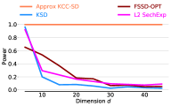
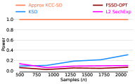
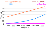
Figure 1: kcc-sd has more power in high dimensions. Left: Gaussian vs Laplace, with $n=1000$ and increasing dimension. Approximate kcc-sd has no loss in power compared to baseline methods. Middle and Right: Gaussian vs Laplace, with $d=30$ and increasing sample size. For all sample sizes studied, approximate kcc-sd has much higher power than the baseline methods, without requiring significantly more compute time.

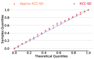
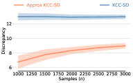
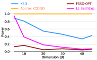
Figure 2: Left: Quantile-Quantile plot showing that kcc-sd and approximate kcc-sd have uniform $p$-values under the null, this was computed with $d=30$ and $n=3000$. Middle: Here we plot the value of kcc-sd and approximate kcc-sd with $p=N(0,I_{d})$ and $q=N(0,\Sigma)$. Here the marginals match but $p\neq q$. As the number of samples increase, both discrepancies stay bounded away from zero. Right: Correlated Gaussian vs Correlated Gaussian with Laplace noise. As the dimension increases kcc-sd does not see a decrease in performance unlike the baseline methods.

Goodness-of-fit Tests.

In the left panel of Figure 1 we compare samples from $q=\prod_{i=1}^{d}\text{Laplace}(0,1/\sqrt{2})$ and target density $p=N(\bm{0},I_{d})$ with increasing dimension. We generate $n=1000$ samples to compute the test statistics, and compute the power of the test over $300$ repetitions with a significance level $\alpha=0.05$. We then observe that as the dimension increases, approximate kcc-sd has power $1$ while other methods see a substantial decrease in power as dimension increases. We show in Appendix F that similar results hold for the imq kernel.

In the middle panel of Figure 1 we plot the power of the test with $q=\prod_{i=1}^{d}\text{Laplace}(0,1/\sqrt{2})$ and $p=N(\bm{0},I_{d})$ with $d=30$. We then increase the number of samples used to compute the test statistics. And in the right panel of Figure 1 we show the time used to compute approximate kcc-sd, ksd, r$\Phi$sd and fssd-opt, the time for approximate kcc-sd also includes the training time for the models. We observe that although approximate kcc-sd requires more time to compute, it has more power than the baselines.

In the left panel of Figure 2 we compare $p=q=N(\bm{0},\Sigma)$ in $d=30$, with $\Sigma_{i,j}=0.5$ for all $i\neq j$ otherwise $\Sigma_{i,i}=1.0$. We show that for $n=3000$ the distribution of the $p$-values is uniform.

In the middle panel of Figure 2, we have $p=N(\bm{0},I_{d})$ and $q=N(\bm{0},\Sigma)$ where $\Sigma_{i,j}=0.5$ for $i\neq j$ and $\Sigma_{i,i}=1$. The figure shows that both kcc-sd and approximate kcc-sd detect the differences between these distributions.

In the right panel of Figure 2, we have $p=N(\bm{0},\Sigma)$ with $\Sigma_{i,j}=0.5$ and $\Sigma_{i,i}=2$ and samples $\bm{x}_{i}=\bm{z}_{i}+\bm{\epsilon}_{i}$, where $\bm{\epsilon}_{i}\sim\prod_{j=1}^{d}\text{Laplace}(0,1/\sqrt{2})$ and $\bm{z}_{i}\sim N(\bm{0},\Sigma_{1})$ with ${(\Sigma_{1})}_{i,j}=0.5$ and ${(\Sigma_{1})}_{i,i}=1$, and $\bm{z}_{i}$ and $\bm{\epsilon}_{i}$ are independent. The samples from $q$ have the same mean and variance as $p$. We compute $n=500$ samples and increase the dimension. As the dimension increases, the power of the test with approximate kcc-sd remains $1$, while the baseline methods see a decline in power.

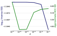
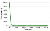
Figure 3: Left: Here, we plot the $\log$ inverse ess for comparison to approximate kcc-sd in assessing quality of samples from sgld. As we can see the inverse ess is minimized at $10^{-3}$, and kcc-sd is minimized at $10^{-5}$. Right: The value of block kcc-sd decreases when the number of iterations goes up in the Gibbs sampler used for Bayesian Probabilistic Matrix Factorization.

Selecting Biased Samplers.

In this experiment we do posterior inference for a three-layer neural network, with a sigmoid activation function, for a regression task. The hidden dimensions are $40$ and $10$. We make use of stochastic gradient Langevin dynamics (sgld), a biased mcmc sampler (Welling and Teh, 2011). We used the yacht hydrodynamics dataset (Gerritsma et al., 1981) from the uci dataset repository. Since biased methods trade sampling efficiency for asymptotic exactness, standard mcmc diagnostics like effective sample size are not applicable as they do not account for asymptotic bias. Selecting the stepsize $\bm{\epsilon}$ is an important task to ensure the samples are approximately from the posterior (Welling and Teh, 2011). For $\bm{\epsilon}\in[10^{-8},10^{-3}]$ we run a chain generating 10,000 samples with a burnin phase of 50,000 samples, with minibatch 256. We compare approximate kcc-sd to effective sample size. The left panel in Figure 3 compares these two metrics. While $\bm{\epsilon}=10^{-6}$ has the lowest kcc-sd value, the inverse effective sample size measure is minimized by the value $\bm{\epsilon}=10^{-2}$.

Detecting Convergence of a Gibbs Sampler for Matrix Factorization.

We assess the convergence of a Gibbs sampler for Bayesian probabilistic matrix factorization (Salakhutdinov and Mnih, 2008). We focus on a variant with two mean parameters $\mu_{V}$ and $\mu_{U}$ for user and movie feature vectors $U_{i}\in\mathbb{R}^{10},V_{j}\in\mathbb{R}^{10}$ and fixed the covariance matrix to the identity (see Appendix F for details).

In this experiment, we chose a subset of the Netflix Prize dataset, with $943$ users and $1682$ movies. We sampled the posterior $p(\bm{\mu}_{U},\bm{\mu}_{V},\bm{U},\bm{V}\mid\bm{R})$ in blocks $\{\mu_{U},\mu_{V},U_{1},\dots,U_{N},V_{1},\dots,V_{M}\}$ by a Gibbs sampler. We ran the sampler for $26$K iterations with no burnin. Since the Gibbs sampler samples blocks of variables together, using these blocks of coordinates to compute kcc-sd is more efficient. In Appendix B we describe block kcc-sd. We compute block kcc-sd by taking every $5^{th}$ sample and show the results in the right panel of Figure 3. As the number of samples increases, block kcc-sd goes down. The sample quality of the Gibbs sample increases with the number of iterations.

6 Discussion

We developed kernelized complete conditional Stein discrepancies and approximate kcc-sd and corresponding goodness-of-fit tests. We show that these discrepancies can distinguish distributions which have smooth and integrable score functions. We also showed empirically that approximate kcc-sd provides a higher power test than those based on ksd. An interesting avenue of research would be relaxing the score function requirement for $q$ and to compare the relative efficiency of the test based on kcc-sd and approximate kcc-sd with baseline methods.

Broader Impact

Our work focuses on comparing distributions where one is known in functional form up to a constant. The primary application of this method lies in probabilistic inference. Improvement in inference could help in building models in domains like healthcare and neuroscience especially to propagate uncertainty about the measurements. However, better inference could also mean better predictive models which can have downsides like in surveillance.

Appendix A Closed Form

Proof.

Define the Stein operator $\mathcal{A}_{p(\bm{x})}$ as follows,

$$(\mathcal{A}_{p(\bm{x})}f)(\bm{x}) =\sum_{j=1}^{d}(\mathcal{A}^{j}_{p(x_{j}\mid\bm{x}_{-j})}f_{j})(\bm{x})=\sum_{j=1}^{d}f_{j}(\bm{x})\nabla_{x_{j}}\log p(\bm{x})+\nabla_{x_{j}}f_{j}(\bm{x})$$

then if for all $j$, $f_{j,\bm{x}_{-j}}$ is in the rkhs of a univariate kernel, $k$, we can use the reproducing property, $f_{j,\bm{x}_{-j}}(x_{j})={\langle{f_{j,\bm{x}_{-j}},k(x_{j},\cdot)}\rangle}_{\mathcal{K}_{k}}$ (Steinwart and Christmann (2008)). Now, define the feature map for each kernel $k_{j}$, $\Phi_{x_{j}}(\cdot)=k(x_{j},\cdot)$, then as

$$\partial_{x_{j}}f_{j,\bm{x}_{-j}}(x_{j}) =\partial_{x_{j}}\langle{f_{j,\bm{x}_{-j}},k(x_{j},\cdot)}\rangle_{\mathcal{K}_{k}}$$

$$=\langle{f_{j,\bm{x}_{-j}},\partial_{x_{j}}k(x_{j},\cdot)}\rangle_{\mathcal{K}_{k}}$$

$$=\langle{f_{j,\bm{x}_{-j}},\partial_{x_{j}}\Phi_{x_{j}}}\rangle_{\mathcal{K}_{k}}$$

then note that we can use the reproducing property for general differential operators, $\mathcal{A}_{p(\bm{x})}^{j}$, to get

$$(\mathcal{A}_{p(x_{j}\mid\bm{x}_{-j})}f_{j})(\bm{x}) =\mathcal{A}_{p(x_{j}\mid\bm{x}_{-j})}\langle{f_{j,\bm{x}_{-j}},k(x_{j},\cdot)}\rangle_{\mathcal{K}_{k}}$$

$$=\langle{f_{j,\bm{x}_{-j}},\mathcal{A}^{j}_{p(x_{j}\mid\bm{x}_{-j})}\Phi_{x_{j}}}\rangle_{\mathcal{K}_{k}}$$

Then we can define the norm of $\mathcal{A}_{p(x_{j}\mid\bm{x}_{-j})}\Phi_{x_{j}}$, as follows:

$$\langle{\mathcal{A}_{p(x_{j}\mid\bm{x}_{-j})}\Phi_{x_{j}},\mathcal{A}_{p(y_{j}\mid\bm{x}_{-j})}\Phi_{y_{j}}}\rangle_{\mathcal{K}_{k}} =b_{j}(x_{j},\bm{x}_{-j})b_{j}(y_{j},\bm{x}_{-j})k(x_{j},y_{j})+\nabla_{x_{j}}\nabla_{y_{j}}k(x_{j},y_{j})$$

$$\qquad+b_{j}(x_{j},\bm{x}_{-j})\nabla_{y_{j}}k(x_{j},y_{j})+b_{j}(y_{j},\bm{x}_{-j})\nabla k(x_{j},y_{j})$$

$$=k^{j}_{cc}(x_{j},y_{j};\bm{x}_{-j})$$ (10)

where $b_{j}(u,\bm{x}_{-j})=\nabla_{u}\log p(u|\bm{x}_{-j})$. Then we define the following

$$w^{2}_{j} =\mathbb{E}_{q(x_{j}\mid\bm{x}_{-j})}\mathbb{E}_{q(y_{j}\mid\bm{x}_{-j})}\left[k_{j}^{cc}(x_{j},y_{j};\bm{x}_{-j})\right]$$

$$=\mathbb{E}_{q(x_{j}\mid\bm{x}_{-j})}\mathbb{E}_{q(y_{j}\mid\bm{x}_{-j})}\left[\langle{\mathcal{A}_{p(x_{j}\mid\bm{x}_{-j})}\Phi_{x_{j}},\mathcal{A}_{p(y_{j}\mid\bm{x}_{-j})}\Phi_{y_{j}}}\rangle_{\mathcal{K}_{k}}\right]$$

$$=\langle{\mathbb{E}_{q(x_{j}\mid\bm{x}_{-j})}\mathcal{A}_{p(x_{j}\mid\bm{x}_{-j})}\Phi_{x_{j}},\mathbb{E}_{q(y_{j}\mid\bm{x}_{-j})}\mathcal{A}_{p(y_{j}\mid\bm{x}_{-j})}\Phi_{y_{j}}}\rangle_{\mathcal{K}_{k}}$$ (11)

$$=\left\lVert\mathbb{E}_{q(x_{j}\mid\bm{x}_{-j})}\mathcal{A}_{p(x_{j}\mid\bm{x}_{-j})}\Phi_{x_{j}}\right\rVert^{2}_{\mathcal{K}_{k}}$$ (12)

where $x_{j},y_{j}\overset{i.i.d}{\sim}q(\cdot\mid\bm{x}_{-j})$ and where we can interchange the inner product and expectation since $\mathcal{A}_{p(x_{j}\mid\bm{x}_{-j})}\Phi_{x_{j}}$ is $q$-Bochner integrable, (Steinwart and Christmann (2008), Definition A.5.20).

We can find the closed form for kcc-sd, where kcc-sd is defined as follows:

$$\mathcal{S}(q,\mathcal{A}_{p},\mathcal{C}_{k}) =\sum_{j=1}^{d}\mathbb{E}_{q(\bm{x}_{-j})}\left[\sup_{f_{j}\in\mathcal{C}_{k}}\left|\mathbb{E}_{q(x_{j}\mid\bm{x}_{-j})}\left[\mathcal{A}_{p(x_{j}\mid\bm{x}_{-j})}^{j}f_{j}(\bm{x})\right]\right|\right]$$

For each $j\in\{1,\dots,d\}$, and $\bm{x}_{-j}$

$$\sup_{f_{j}\in\mathcal{C}_{k}}\mathbb{E}_{q(x_{j}\mid\bm{x}_{-j})}\left[\mathcal{A}_{p(x_{j}\mid\bm{x}_{-j})}^{j}f_{j}(x)\right] =\sup_{f_{j}:\left\lVert f_{j}\right\rVert\leq w_{j}^{2}}\langle{f_{j},\mathbb{E}_{q(x_{j}\mid\bm{x}_{-j})}}\left[\mathcal{A}_{p(x_{j}\mid\bm{x}_{-j})}\Phi_{x_{j}}\right]\rangle_{\mathcal{K}_{k}}$$

$$=\left\lVert\mathbb{E}_{q(x_{j}\mid\bm{x}_{-j})}\mathcal{A}_{p(x_{j}\mid\bm{x}_{-j})}\Phi_{x_{j}}\right\rVert^{2}_{\mathcal{K}_{k}}$$

$$=\mathbb{E}_{q(x_{j}\mid\bm{x}_{-j})}\mathbb{E}_{q(y_{j}\mid\bm{x}_{-j})}\left[k^{j}_{cc}(x_{j},y_{j};\bm{x}_{-j})\right]$$

hence, kcc-sd can be written in closed form as

$$\mathcal{S}(q,\mathcal{A}_{p},\mathcal{C}_{k})=\sum_{j=1}^{d}\mathbb{E}_{q(\bm{x}_{-j})}\mathbb{E}_{q(x_{j}\mid\bm{x}_{-j})}\mathbb{E}_{q(y_{j}\mid\bm{x}_{-j})}\left[k^{j}_{cc}(x_{j},y_{j};\bm{x}_{-j})\right]$$

∎

Here, we show that kcc-sds can be expressed as an average of univariate ksds. We can compute the Stein kernel for kcc-sd as

$$k_{cc}^{j}(x_{j},y_{j};\bm{x}_{-j}) =k(x_{j},y_{j})b_{j}(x_{j},\bm{x}_{-j})b_{j}(y_{j},\bm{x}_{-j})+\nabla_{x_{j}}k(x_{j},y_{j})b_{j}(y_{j},\bm{x}_{-j})$$

$$\qquad+\nabla_{y_{j}}k(x_{j},y_{j})b_{j}(x_{j},\bm{x}_{-j})+\nabla_{x_{j}}\nabla_{y_{j}}k(x_{j},y_{j}),$$

$$=\left(\mathcal{A}_{p(x_{j}\mid\bm{x}_{-j})}\mathcal{A}_{p(y_{j}\mid\bm{x}_{-j})}k\right)(x_{j},y_{j})$$

where $\bm{x}_{-j}\in\mathbb{R}^{d-1}$ is fixed, $k:\mathbb{R}\times\mathbb{R}\rightarrow\mathbb{R}$, and $b_{j}(x_{j},\bm{x}_{-j})=\nabla_{x_{j}}\log p(x_{j}\mid\bm{x}_{-j})$. Using the Stein kernel defined above we can compute ksd between $p(\cdot\mid\bm{x}_{-j})$ and $q(\cdot\mid\bm{x}_{-j})$ as follows

$$\mathcal{S}{\left(q(\cdot\mid\bm{x}_{-j}),\mathcal{A}_{p(\cdot\mid\bm{x}_{-j})},\mathcal{G}_{k}\right)}^{2} =\mathbb{E}_{q(x_{j}\mid\bm{x}_{-j})}\mathbb{E}_{q(y_{j}\mid\bm{x}_{-j})}\left[\left(\mathcal{A}_{p(x_{j}\mid\bm{x}_{-j})}\mathcal{A}_{p(y_{j}\mid\bm{x}_{-j})}k\right)(x_{j},y_{j})\right]$$

$$=\mathbb{E}_{q(x_{j}\mid\bm{x}_{-j})}\mathbb{E}_{q(y_{j}\mid\bm{x}_{-j})}\left[k_{cc}^{j}(x_{j},y_{j};\bm{x}_{-j})\right].$$

Therefore, kcc-sd can also be computed as

$$\mathcal{S}(q,\mathcal{A}_{p},\mathcal{C}_{k}) =\sum_{j=1}^{d}\mathbb{E}_{q(\bm{x}_{-j})}\mathbb{E}_{q(x_{j}\mid\bm{x}_{-j})}\mathbb{E}_{q(y_{j}\mid\bm{x}_{-j})}\left[k^{j}_{cc}(x_{j},y_{j};\bm{x}_{-j})\right]$$

$$=\sum_{j=1}^{d}\mathbb{E}_{q(\bm{x}_{-j})}\left[\mathcal{S}{\left(q(\cdot\mid\bm{x}_{-j}),\mathcal{A}_{p(\cdot\mid\bm{x}_{-j})},\mathcal{G}_{k}\right)}^{2}\right].$$

In Algorithm 1 we show how to compute kcc-sd exactly when we have samples from the complete conditionals.

Input: Dataset ${\{\bm{x}^{(i)}\}}_{i=1}^{n}$, $d$: dimension of $\bm{x}$, $n_{y}$: number of $y_{j}$ samples and complete conditionals $q(\cdot\mid\bm{x}_{-j})$

Output: Estimated kcc-sd $\hat{S}_{n}(q,\mathcal{A}_{p},\mathcal{C}_{k})$

for $j\in[d]$ do

       for $i\in[n]$ do

             Sample $y^{(i,k)}_{j}\sim q(\cdot\mid\bm{x}^{(i)}_{-j})$ for $k\in[n_{y}]$

            

       end for

      Let $\hat{w}^{2}_{j}=\frac{1}{nn_{y}}\sum_{i=1}^{n}\sum_{k=1}^{n_{y}}k_{cc}^{j}(x_{j}^{(i)},y_{j}^{(i,k)};\bm{x}^{(i)}_{-j})$

      

end for

Let $\hat{S}_{n}(q,\mathcal{A}_{p},\mathcal{C}_{k})=\sum_{j=1}^{d}\hat{w}^{2}_{j}$

Algorithm 1 Computing KCC-SDs with complete conditionals

Appendix B kcc-sd in practice

Input: Dataset $\mathcal{D}={\{\bm{x}^{(i)}\}}_{i=1}^{n}$, $d$: dimension of $\bm{x}$, $n_{y}$: number of $y_{j}$ samples, and a model class $r_{\lambda_{j}}(\cdot\mid\bm{x}_{-j})$ for each complete conditional.

Output: Approximate kcc-sd

Split the dataset into training, validation and test sets.

for $j\in[d]$ do

        Train the sampler $r_{\lambda_{j}}$ on training set.

        Select the model $r_{\lambda_{j}}$ with lowest validation loss.

       for $i\in[n]$ do

             Sample $y^{(i,l)}_{j}\sim r_{\lambda_{j}}(\cdot\mid\bm{x}^{(i)}_{-j})$ for $l\in[n_{y}]$

            

       end for

       Let $\hat{w}^{2}_{j}=\frac{1}{n}\sum_{i=1}^{n}\frac{1}{n_{y}}\sum_{l=1}^{n_{y}}k_{cc}(x_{j}^{(i)},y_{j}^{(i,l)};\bm{x}^{(i)}_{-j})$.

end for

Let $\hat{S}_{\lambda}(q,\mathcal{A}_{p},\mathcal{C}_{k})=\sum_{j=1}^{d}\hat{w}^{2}_{j}$

Algorithm 2 Computing approximate KCC-SDs. Given model class $r_{\lambda_{j}}$, compute approximate kcc-sd.

Block kcc-sd.

In Gibbs sampling, when variables are sampled together, using blocks of coordinates to compute kcc-sd will be computationally more efficient than using single coordinates. The complete conditional approach still ensures that block kcc-sd distinguishes the distributions $p$ and $q$. For instance, if $\bm{x}\in\mathbb{R}^{d}$, then let $I_{1},\dots,I_{m}$ be disjoint partitions of indices $\{1,\dots,d\}$ such that $\cup_{j=1}^{m}I_{j}=\{1,\dots,d\}$, then we can define block kcc-sd as

$$\sum_{j=1}^{m}\mathbb{E}_{q(\bm{x}_{-I_{j}})}\sup_{f_{I_{j}}}\mathbb{E}_{q(\bm{x}_{I_{j}}\mid\bm{x}_{-I_{j}})}[\mathcal{A}^{j}_{p(\bm{x}_{I_{j}}\mid\bm{x}_{-I_{j}})}f_{I_{j}}(\bm{x})]\ ,$$

here the the dimension of the kernel would depend on the block size, so $k_{j}:\mathbb{R}^{I_{j}}\times\mathbb{R}^{I_{j}}\rightarrow\mathbb{R}$. The supremum of the block kcc-sd is

$$\sum_{j=1}^{m}\mathbb{E}_{q(\bm{x}_{-I_{j}})}\mathbb{E}_{\bm{x}_{I_{j}},\bm{y}_{I_{j}}\sim q(\cdot\mid\bm{x}_{-I_{j}})}\left[k_{cc}^{j}(\bm{x}_{I_{j}},\bm{y}_{I_{j}};\bm{x}_{-I_{j}})\right]\ .$$

Note that if we take all the coordinates as one block, block kcc-sd is equivalent to ksd.

Appendix C Distinguishing Distributions

Here, we rely on the ispd property of the kernel $k(x_{j},y_{j})$ so that for any function $f:\mathbb{R}\rightarrow\mathbb{R}$, we obtain

$$\int_{u\in\mathbb{R}}\int_{v\in\mathbb{R}}f(u)k(u,v)f(v)dudv>0$$

for $\left\lVert f\right\rVert>0$.

Note that we can write the Stein discrepancy as,

$$\mathbb{E}_{q(\bm{x})}\left[\mathcal{A}_{p(\bm{x})}f(\bm{x})\right] =\mathbb{E}_{q(\bm{x})}\left[\mathcal{A}_{p(\bm{x})}f(y)-\mathcal{A}_{q(\bm{x})}f(\bm{x})\right]$$

$$=\mathbb{E}_{q(\bm{x})}\left[{f(\bm{x})}^{T}\nabla_{\bm{x}}\log p(\bm{x})+\nabla_{\bm{x}}\cdot f(\bm{x})\right]-\mathbb{E}_{q(\bm{x})}\left[{f(\bm{x})}^{T}\nabla_{\bm{x}}\log q(\bm{x})+\nabla_{\bm{x}}\cdot f(\bm{x})\right]$$

$$=\mathbb{E}_{q(\bm{x})}\left[{f(\bm{x})}^{T}\left(\nabla_{\bm{x}}\log p(\bm{x})-\log q(\bm{x})\right)\right]$$

$$=\mathbb{E}_{q(\bm{x})}\left[{f(\bm{x})}^{T}\nabla_{\bm{x}}\log\frac{p(\bm{x})}{q(\bm{x})}\right]\ ,$$ (13)

using $\mathbb{E}_{q(\bm{x})}\left[\mathcal{A}_{q(\bm{x})}f(\bm{x})\right]=0$.

Using this representation for our test function, $f^{*}_{j}(\bm{x})=\mathbb{E}_{q(y_{j}\mid\bm{x}_{-j})}[\mathcal{A}_{p(y_{j}|\bm{x}_{-j})}^{j}k(x_{j},y_{j})]$, where $y_{j}\sim q(\cdot\mid\bm{x}_{-j})$, we see that

$$f^{*}_{j}(\bm{x}) =\mathbb{E}_{q(y_{j}\mid\bm{x}_{-j})}[\mathcal{A}_{p(y_{j}|\bm{x}_{-j})}^{j}k(x_{j},y_{j})]-\mathbb{E}_{q(y_{j}\mid\bm{x}_{-j})}[\mathcal{A}_{q(y_{j}|\bm{x}_{-j})}^{j}k(x_{j},y_{j})]$$

$$=\mathbb{E}_{q(y_{j}\mid\bm{x}_{-j})}\left[k(x_{j},y_{j})\nabla_{y_{j}}\log\frac{p(y_{j}\mid\bm{x}_{-j})}{q(y_{j}\mid\bm{x}_{-j})}\right]$$

$$=\mathbb{E}_{q(y_{j}\mid\bm{x}_{-j})}\left[k(x_{j},y_{j})\nabla_{y_{j}}\log\frac{p(y_{j},\bm{x}_{-j})}{q(y_{j},\bm{x}_{-j})}\right]\ ,$$ (14)

then using the fact that $\mathcal{S}(q,\mathcal{A}_{p},\mathcal{C}_{k})=\sum_{j=1}^{d}\mathbb{E}_{q(\bm{x})}[\mathcal{A}_{p(\bm{x})}^{j}f_{j}^{*}(\bm{x})]$, we obtain using Eq. 13 and Eq. 14

$$\mathcal{S}(q,\mathcal{A}_{p},\mathcal{C}_{k}) =\mathbb{E}_{q(\bm{x})}\left[{f^{*}(\bm{x})}^{T}\nabla_{\bm{x}}\log\frac{p(\bm{x})}{q(\bm{x})}\right]$$

$$=\sum_{j=1}^{d}\mathbb{E}_{q(\bm{x}_{-j})}\left[\mathbb{E}_{q(x_{j}\mid\bm{x}_{-j})}\left[f^{*}_{j}(\bm{x})\nabla_{x_{j}}\log\frac{p(\bm{x})}{q(\bm{x})}\right]\right]$$

$$=\sum_{j=1}^{d}\mathbb{E}_{q(\bm{x}_{-j})}\left[\mathbb{E}_{q(x_{j}\mid\bm{x}_{-j})}\mathbb{E}_{q(y_{j}\mid\bm{x}_{-j})}\left[\nabla_{y_{j}}\log\frac{p(y_{j},\bm{x}_{-j})}{q(y_{j},\bm{x}_{-j})}k(x_{j},y_{j})\nabla_{x_{j}}\log\frac{p(\bm{x})}{q(\bm{x})}\right]\right]\ .$$

Now, observe that for each $j\in\{1,\dots,d\}$, with $r(u,\bm{x}_{-j})=\nabla_{u}\log\frac{p(u,\bm{x}_{-j})}{q(u,\bm{x}_{-j})}$, we define a function $h$ over $\bm{x}_{-j}$

$$h(\bm{x}_{-j}) =\mathbb{E}_{q(x_{j}\mid\bm{x}_{-j})}\mathbb{E}_{q(y_{j}\mid\bm{x}_{-j})}\left[\nabla_{y_{j}}\log\frac{p(y_{j},\bm{x}_{-j})}{q(y_{j},\bm{x}_{-j})}k(x_{j},y_{j})\nabla_{x_{j}}\log\frac{p(\bm{x})}{q(\bm{x})}\right]$$

$$=\mathbb{E}_{q(x_{j}\mid\bm{x}_{-j})}\mathbb{E}_{q(y_{j}\mid\bm{x}_{-j})}\left[r(y_{j},\bm{x}_{-j})k(x_{j},y_{j})r(x_{j},\bm{x}_{-j})\right]$$

$$=\int_{x_{j}}\int_{y_{j}}q(x_{j}\mid\bm{x}_{-j})r(x_{j},\bm{x}_{-j})k(x_{j},y_{j})q(y_{j}\mid\bm{x}_{-j})r(y_{j},\bm{x}_{-j})dx_{j}dy_{j}$$

$$=\int_{x_{j}}\int_{y_{j}}g_{\bm{x}_{-j}}(x_{j})k(x_{j},y_{j})g_{\bm{x}_{-j}}(y_{j})dx_{j}dy_{j}$$ (15)

where $g_{\bm{x}_{-j}}(u)=q(u\mid\bm{x}_{-j})r(u,\bm{x}_{-j})=q(u\mid\bm{x}_{-j})\nabla_{u}\log\frac{p(u,\bm{x}_{-j})}{q(u,\bm{x}_{-j})}$.

The proofs in this section rely on the next lemma, which states that if the complete conditionals match, then the distributions also match.

Lemma 2.

If $p(\bm{x})$, $q(\bm{x})>0$ for all $\bm{x}\in\mathbb{R}^{d}$ and $p(x_{j}|\bm{x}_{-j})=q(x_{j}|\bm{x}_{-j})$ for all $\bm{x}_{-j}$ and $j$, then $p(\bm{x})=q(\bm{x})$.

Proof (Lemma 2).

We prove by induction. If dimension of $x$ is 2, then $p(x_{1}|x_{2})=q(x_{1}|x_{2})$ and $p(x_{2}|x_{1})=q(x_{2}|x_{1})$. Then we have

$$\int\frac{p(x_{1}|x_{2})}{p(x_{2}|x_{1})}dx_{1}=\int\frac{p(x_{1})}{p(x_{2})}dx_{1}=\frac{1}{p(x_{2})},$$

and

$$\int\frac{q(x_{1}|x_{2})}{q(x_{2}|x_{1})}dx_{1}=\int\frac{q(x_{1})}{q(x_{2})}dx_{1}=\frac{1}{q(x_{2})},$$

which implies

$$\frac{1}{p(x_{2})}=\int\frac{p(x_{1}|x_{2})}{p(x_{2}|x_{1})}dx_{1}=\int\frac{q(x_{1}|x_{2})}{q(x_{2}|x_{1})}dx_{1}=\frac{1}{q(x_{2})}.$$

Therefore, $p(x_{2})=q(x_{2})$ for all $x_{2}$.$p(x_{1},x_{2})=p(x_{1}|x_{2})p(x_{2})=q(x_{1}|x_{2})q(x_{2})=q(x_{1},x_{2})$.

Assume the dimension of $\bm{x}$ is $d$. Then we have

$$\frac{p(\bm{x}_{-\{i,j\}})}{p(\bm{x}_{-i})}=\int\frac{p(\bm{x}_{-j})}{p(\bm{x}_{-i})}dx_{i}=\int\frac{p(x_{i}|\bm{x}_{-i})}{p(x_{j}|\bm{x}_{-j})}dx_{i}=\int\frac{q(x_{i}|\bm{x}_{-i})}{q(x_{j}|\bm{x}_{-j})}dx_{i}=\int\frac{q(\bm{x}_{-j})}{q(\bm{x}_{-i})}dx_{i}=\frac{q(\bm{x}_{-\{i,j\}})}{q(\bm{x}_{-i})}$$

for all $j$. Then $p(\bm{x}_{j}|\bm{x}_{-\{i,j\}})=q(\bm{x}_{j}|\bm{x}_{-\{i,j\}})$ for all $j$. Since $\bm{x}_{-i}$ is a $(d-1)$ dimensional distribution, we can use the induction. Since $p(\bm{x}_{j}|\bm{x}_{-\{i,j\}})=q(\bm{x}_{j}|\bm{x}_{-\{i,j\}})$ for all $j$, by induction, we have $p(\bm{x}_{-i})=q(\bm{x}_{-i})$. Therefore,

$$p(\bm{x})=p(x_{i}|\bm{x}_{-i})p(\bm{x}_{-i})=q(x_{i}|\bm{x}_{-i})q(\bm{x}_{-i})=q(\bm{x}).$$

∎

Using Equation 13 we can see that if $p\overset{d}{=}q$, then $\mathbb{E}_{q}[\mathcal{A}_{p}f(\bm{x})]=0$ for $f$ integrable and smooth. The Stein set for kcc-sd, $\mathcal{C}_{k}$, consists of such functions. We restate Theorem 2 for clarity.

Theorem.

Suppose $k\in C^{2,2}(\mathbb{R},\mathbb{R})$ is an ispd kernel and $\mathbb{E}_{q(\bm{x})}[\left\|\nabla_{\bm{x}}\log p(\bm{x})\right\|^{2}],\mathbb{E}_{q(\bm{x})}[\left\|\nabla_{\bm{x}}\log q(\bm{x})\right\|^{2}]<\infty$ where $p(\bm{x}),q(\bm{x})>0$ for all $\bm{x}\in\mathbb{R}^{d}$. If $p\overset{d}{=}q$, then $\mathcal{S}(q,\mathcal{A}_{p},\mathcal{C}_{k})=0$.

Proof (Theorem 2).

If $p\overset{d}{=}q$, then the score functions match and using Equation 13, for all $f$ such that $\mathbb{E}_{q(\bm{x})}\|f(\bm{x})\|_{2}<\infty$, then

$$\mathbb{E}_{q(\bm{x})}\left[\mathcal{A}_{p(\bm{x})}f(\bm{x})\right] =\mathbb{E}_{q(\bm{x})}\left[{f(\bm{x})}^{T}\nabla_{\bm{x}}\log\frac{p(\bm{x})}{q(\bm{x})}\right]$$

$$=0$$

Since all $f\in\mathcal{C}_{k}$ satisfy $\mathbb{E}_{q(\bm{x})}\|f(\bm{x})\|_{2}<\infty$, $\mathcal{S}(q,\mathcal{A}_{p},\mathcal{C}_{k})=0$.

∎

Similarly, using Equation 13 we can show that when $p\neq q$, then kcc-sd will be strictly greater than zero. This relies on the fact that if two measures are not equal, then on the set where they are not equal, the complete conditionals will not match. We can exploit this property to show that kcc-sd will not be zero for such distributions. We restate Theorem 3 for clarity.

Theorem 4.

Let $k$ be integrally strictly positive definite. Suppose if $\mathcal{S}(q,\mathcal{A}_{p},\mathcal{C}_{k})<\infty$, and $\mathbb{E}_{q(\bm{x})}[\left\|\nabla_{\bm{x}}\log p(\bm{x})\right\|^{2}],\mathbb{E}_{q(\bm{x})}[\left\|\nabla_{\bm{x}}\log q(\bm{x})\right\|^{2}]<\infty$ with $p(\bm{x}),q(\bm{x})>0$, then if $p$ is not equal to $q$ in distribution, then $\mathcal{S}(q,\mathcal{A}_{p},\mathcal{C}_{k})>0$.

Proof (Theorem 3).

Suppose $p\neq q$ in distribution, then by Lemma 2 there exists a $j\in\{1,\dots,d\}$ and a set $B_{-j}\subset\mathbb{R}^{d-1}$, with $m_{d-1}(B_{-j})>0$ where $m_{d-1}$ is Lebesgue measure, such that for each $\bm{x}_{-j}\in B_{-j}$ there exists a set $A_{j,\bm{x}_{-j}}\subset\mathbb{R}$ with $m_{1}(A_{j,\bm{x}_{-j}})>0$, where the complete conditional do not match. Then as the complete conditionals, $p(x_{j}\mid\bm{x}_{-j}),q(x_{j}\mid\bm{x}_{-j})$, do not match on $A_{j,\bm{x}_{-j}}$, the ratio of the score functions do not match, so for $\bm{x}_{-j}\in B_{-j}$ and $u\in A_{j,\bm{x}_{-j}}$,

$$g_{\bm{x}_{-j}}(u)=q(u\mid\bm{x}_{-j})\nabla_{x_{j}}\log\frac{p(u,\bm{x}_{-j})}{q(u,\bm{x}_{-j})}\neq 0\ .$$

As $q$ has full support, for all $\bm{x}_{-j}\in B_{-j}$ we have $g_{\bm{x}_{-j}}(u)\neq 0$ on $A_{j,\bm{x}_{-j}}$, this implies that the $L_{2}$ norm of this function is not zero, $\left\lVert g_{\bm{x}_{-j}}\right\rVert_{2}\neq 0$. Thus, for $\bm{x}_{-j}\in B_{-j}$, by the ispd property of the kernel,

$$h(\bm{x}_{-j})=\int_{x_{j}}\int_{y_{j}}g_{\bm{x}_{-j}}(x_{j})k(x_{j},y_{j})g_{\bm{x}_{-j}}(y_{j})dx_{j}dy_{j}>0$$

and since $m_{d-1}(B_{-j})$, $\mathbb{E}_{q(\bm{x}_{-j})}[h(\bm{x}_{-j})]>0$. Thus, $\mathcal{S}(q,\mathcal{A}_{p},\mathcal{C}_{k})>0$. ∎

Appendix D Proof of Lemma 4: Bounding the gap in approximate kcc-sd

To prove Lemma 4 we make use of the following lemma (Gorham and Mackey, 2017) to bound the difference between the expectation of the Stein operator on different distributions.

Lemma 3.

Suppose $\nabla_{\bm{x}}\log p(\bm{x})$ is Lipschitz and $L_{2}(q)\cap L_{2}(r)$, and $f$ and $\nabla_{\bm{x}}f$ are uniformly bounded and Lipschitz, then we can show that

$$\left|\mathbb{E}_{q(\bm{x})}[\mathcal{A}_{p(\bm{x})}f(\bm{x})]-\mathbb{E}_{r(\bm{y})}[\mathcal{A}_{p(\bm{y})}f(\bm{y})]\right|\leq K_{1}W_{2}(q,r)+\sqrt{K_{2}W_{2}(q,r)},$$

where $K_{1},K_{2}$ are positive constants.

Proof.

Suppose the score function, $s_{p}(\bm{x})=\nabla_{\bm{x}}\log p(\bm{x})$, is Lipschitz and the function $f$ is bounded with a Lipschitz derivative then we can bound the approximation error as follows

$$\left|\mathbb{E}_{q(\bm{x})}\left[\mathcal{A}_{p(\bm{x})}f(\bm{x})\right]-\mathbb{E}_{r(\bm{y})}\left[\mathcal{A}_{p(\bm{y})}f(\bm{y})\right]\right|\leq \left|\mathbb{E}_{q(\bm{x})}\left[f(\bm{x})^{T}s_{p}(\bm{x})\right]-\mathbb{E}_{r(\bm{y})}\left[f(\bm{y})^{T}s_{p}(\bm{y})\right]\right|$$

$$\qquad\qquad+\left|\mathbb{E}_{q(\bm{x})}\nabla_{\bm{x}}\cdot f(\bm{x})-\mathbb{E}_{r(\bm{y})}\nabla_{\bm{y}}\cdot f(\bm{y})\right|$$

Now, assume that $f$ is bounded and $\nabla\log p$ is Lipschitz and so is $\nabla_{\bm{x}}f$. Then, we can bound the second term above as follows

$$\left|\mathbb{E}_{q(\bm{x})}\nabla_{\bm{x}}\cdot f(\bm{x})-\mathbb{E}_{r(\bm{y})}\nabla_{\bm{y}}\cdot f(\bm{y})\right|\leq L(\nabla f)\mathbb{E}[{\left\lVert\bm{x}-\bm{y}\right\rVert_{2}}],$$

where $L(h)$ is the Lipschitz constant of the function $h$ and $B(h)=\sup_{\bm{x}}\left\lVert h(\bm{x})\right\rVert_{2}$.

Similarly, we split the first term as follows

$$\left|\mathbb{E}_{q(\bm{x})}\left[f(\bm{x})^{T}s_{p}(\bm{x})\right]-\mathbb{E}_{r(\bm{y})}\left[f(\bm{y})^{T}s_{p}(\bm{y})\right]\right| \leq\left|\mathbb{E}\left[f(\bm{x})^{T}\left(s_{p}(\bm{x})-s_{p}(\bm{y})\right)\right]\right|$$

$$\quad\quad+\left|\mathbb{E}[s_{p}(\bm{y})^{T}(f(\bm{y})-f(\bm{x}))]\right|.$$

We can then bound the first term above using the fact that the function $f$ is bounded and the score function is Lipschitz.

$$\left|\mathbb{E}\left[f(\bm{x})^{T}\left(s_{p}(\bm{x})-s_{p}(\bm{y})\right)\right]\right|\leq B(f)L(\nabla\log p)\mathbb{E}[\left\lVert\bm{x}-\bm{y}\right\rVert_{2}]$$

and similarly we can bound the second term by using the fact that the function $f$ is bounded and Lipschitz and the the score function is square integrable,

$$\left|\mathbb{E}[s_{p}(\bm{y})^{T}(f(\bm{y})-f(\bm{x}))]\right| \leq\mathbb{E}[\left\lVert f(\bm{y})-f(\bm{x})\right\rVert_{2}\left\lVert s_{p}(\bm{y})\right\rVert_{2}]$$

$$\leq\mathbb{E}\left[\min\left(2B(f),L(f)\left\lVert\bm{x}-\bm{y}\right\rVert_{2}\right)\left\lVert s_{p}(\bm{y})\right\rVert\right]$$

and then using the fact that $\min(a,b)\leq\sqrt{ab}$ for $a,b\geq 0$, and applying Cauchy-Schwarz again we obtain

$$\left|\mathbb{E}[s_{p}(\bm{y})^{T}(f(\bm{y})-f(\bm{x}))]\right| \leq\sqrt{2B(f)L(f)}\mathbb{E}\left[\left\lVert\bm{x}-\bm{y}\right\rVert_{2}^{\frac{1}{2}}\left\lVert s_{p}(\bm{y})\right\rVert_{2}\right]$$

$$\leq\sqrt{2B(f)L(f)}\sqrt{\mathbb{E}\left[\left\lVert\bm{x}-\bm{y}\right\rVert_{2}\right]\mathbb{E}\left[\left\lVert s_{p}(\bm{y})\right\rVert_{2}^{2}\right]}.$$

We can then bound the all the terms by

$$\left|\mathbb{E}_{q(\bm{x})}[\mathcal{A}_{p(\bm{x})}f(\bm{x})]-\mathbb{E}_{r(\bm{y})}[\mathcal{A}_{p(\bm{y})}f(\bm{y})]\right|\leq K_{1}\mathbb{E}\left[\left\lVert\bm{x}-\bm{y}\right\rVert_{2}\right]+\sqrt{K_{2}\mathbb{E}[\left\lVert\bm{x}-\bm{y}\right\rVert_{2}]},$$

where $K_{1}=L(\nabla f)+B(f)L(\nabla\log p)$ and $K_{2}=2B(f)L(f)\mathbb{E}_{r}[\left\lVert s_{p}(\bm{y})\right\rVert_{2}]$ are constants. Now, by taking the infimum over all joint distributions $P$ on $\bm{x}$ and $\bm{y}$, where the marginals match with $q$ and $r$, we obtain

$$\left|\mathbb{E}_{q(\bm{x})}[\mathcal{A}_{p(\bm{x})}f(\bm{x})]-\mathbb{E}_{r(\bm{y})}[\mathcal{A}_{p(\bm{y})}f(\bm{y})]\right|\leq K_{1}W_{2}(q,r)+\sqrt{K_{2}W_{2}(q,r)},$$

where the Wasserstein distance is defined as $W_{2}(p,q)=\inf_{P,\bm{x}\sim p,\bm{y}\sim q}\mathbb{E}_{P}\left[\left\lVert\bm{x}-\bm{y}\right\rVert_{2}\right]$.

∎

Suppose a distribution $q$ satisfies a $\rho$-transport inequality (Definition 3.58, (Wainwright, 2019)), then for any distribution $p$ we have the following inequality

$$W_{2}(q,p)\leq\sqrt{2\rho^{2}D(p,q)},$$ (16)

where $D$ is the kl divergence. We make use of the $\rho$-transport inequality to bound the Wasserstein-$2$ in the bound proved in Lemma 3.

For brevity we refer to the complete conditional $q(x_{j}\mid\bm{x}_{-j})$ as $q_{\mid\bm{x}_{-j}}(x_{j})$. And we restate Lemma 4 below for reference.

Lemma 4.

Suppose the model class $r_{\lambda_{j}}$ satisfies a $\rho$-transport inequality and $\nabla_{\bm{x}}\log p(\bm{x})$ is Lipschitz and $\mathbb{E}_{q}[\left\lVert\nabla_{\bm{x}}\log p(\bm{x})\right\rVert],\mathbb{E}_{r_{\lambda_{j}}}[\left\lVert\nabla_{x_{j}}\log p(\bm{x}\mid\bm{x}_{-j})\right\rVert]<\infty$, and the kernel $k$ is bounded with $\nabla_{x_{j}}k(x_{j},y_{j})$ Lipschitz, then

$$\left|\mathcal{S}(q,\mathcal{A}_{p},\mathcal{C}_{k})-\mathcal{S}_{\lambda}(q,\mathcal{A}_{p},C_{k})\right|\leq\sum_{j=1}^{d}K_{1,j}\sqrt{2\rho^{2}\epsilon_{j}}+\sqrt{K_{2,j}\sqrt{2\rho^{2}\epsilon_{j}}}$$

where $\sup_{\bm{x}_{-j}}\textsc{kl}(q(\cdot|\bm{x}_{-j})\mid\mid r_{\lambda_{j}})<\epsilon_{j}$ and $K_{1,j},K_{2,j}$ are positive constants.

Proof of Lemma 4.

Suppose the complete conditionals $r_{\lambda_{j}}$ satisfy a $\rho$-transport inequality Equation 16. Then suppose $f$ is bounded and has a Lipschitz derivative then using Lemma 3 we get the following bound for each $j$,

$$\left|\mathbb{E}_{q(x_{j}\mid\bm{x}_{-j})}[\mathcal{A}_{p(x_{j}\mid\bm{x}_{-j})}f(x_{j})]-\mathbb{E}_{r_{\lambda_{j}}(y_{j}\mid\bm{x}_{-j})}[\mathcal{A}_{p(y_{j}\mid\bm{x}_{-j})}f(y_{j})]\right| \leq K_{1,j}W_{2}(r_{\lambda_{j}},q)+\sqrt{K_{2,j}W_{2}(r_{\lambda_{j}},q)}$$

$$\leq K_{1,j}\sqrt{2\rho^{2}D(q_{\mid\bm{x}_{-j}},r_{\lambda_{j}})}$$

$$\quad\quad+\sqrt{K_{2,j}\sqrt{2\rho^{2}D(q_{\mid\bm{x}_{-j}},r_{\lambda_{j}})}}.$$

Note Lemma 4 follows from Lemma 3 as the function $h(y_{j})=\mathbb{E}_{q(x_{j}\mid\bm{x}_{-j})}[\mathcal{A}_{p(x_{j}\mid\bm{x}_{-j})}k(x_{j},y_{j})]$ satisfies the boundedness and Lipschitz assumption for Lemma 3. Therefore, we can show that if $\epsilon_{j}=\sup_{\bm{x}_{-j}}\textsc{kl}(q_{\mid\bm{x}_{-j}},r_{\lambda_{j}})$ then

$$\left|\mathcal{S}(q,\mathcal{A}_{p},\mathcal{C}_{k})-\mathcal{S}_{\lambda}(q,\mathcal{A}_{p},C_{k})\right| \leq\sum_{j=1}^{d}\mathbb{E}_{q(\bm{x}_{-j})}\left|\mathbb{E}_{r_{\lambda_{j}}(z_{j}\mid\bm{x}_{-j})}\mathcal{A}_{p}h(z_{j})-\mathbb{E}_{q(y_{j}\mid\bm{x}_{-j})}\mathcal{A}_{p}h(y_{j})\right|$$

$$\leq\sum_{j=1}^{d}K_{1,j}\sqrt{\epsilon_{j}}+\sqrt{K_{2,j}\sqrt{2\rho^{2}\epsilon_{j}}}.$$

∎

Appendix E Goodness of fit Testing

In this section we show that

1. When the null hypothesis is true, the bootstrapped statistics can be used to approximate quantile of the null distribution, so

   $$\sup_{\beta}\left|\mathbb{P}\left[\sqrt{n}T_{n}>\beta\right]-\mathbb{P}\left[\sqrt{n}R_{n}>\beta\mid{\{\bm{x}^{(i)}\}}_{i\leq n}\right]\right|\rightarrow 0$$

   as $n\rightarrow\infty$. This holds when the test statistic is computed using either kcc-sd or approximate kcc-sd.

2. When the alternate hypothesis is true, the test statistic computed using kcc-sd converges to a positive constant almost surely (Theorem 3), that is $\mathbb{P}[T_{n}>0]\rightarrow 1$. And this leads to an almost sure rejection of the null asymptotically.

3. When the alternate hypothesis holds, the asymptotic behaviour of the test with approximate kcc-sd depends on the model $r_{\lambda_{j}}$.

The goodness-of-fit test using approximate kcc-sd makes use of the fact that approximate kcc-sd converges to zero as the number of samples increases, this can be seen immediately using Stein’s identity. Stein’s identity states that for bounded functions $f$ with a bounded derivative (Proposition 1, Gorham and Mackey (2015)), which vanish at infinity,

$$\mathbb{E}_{p(\bm{x})}\left[\mathcal{A}_{p(\bm{x})}f(\bm{x})\right]=0.$$

Using Stein’s identity we show that when $p=q$, approximate kcc-sd, $S_{\lambda}(q,\mathcal{A}_{p},\mathcal{C}_{k})$, is zero.

Lemma 5.

Suppose $k$ is bounded and twice differentiable in both arguments with bounded derivatives and both $k(x_{j},y_{j})$ and $\nabla_{x_{j}}k(x_{j},y_{j}),\nabla_{y_{j}}k(x_{j},y_{j})$ vanish at infinity, and the score function $\nabla_{y_{j}}\log p(y_{j}\mid\bm{x}_{-j})\in L_{2}(r_{\lambda_{j}})$ for $q(\bm{x}_{-j})$ almost surely and $r_{\lambda_{j}}$ is a density and $\mathbb{E}_{q(\bm{x})}[\left\lVert\nabla_{\bm{x}}\log p(\bm{x})\right\rVert^{2}_{2}],\mathbb{E}_{q(\bm{x})}[\left\lVert\nabla_{\bm{x}}\log q(\bm{x})\right\rVert^{2}_{2}]<\infty$. Then if $p=q$, we have the following

$$\mathcal{S}_{\lambda}(q,\mathcal{A}_{p},\mathcal{C}_{k})=\sum_{j=1}^{d}\mathbb{E}_{q(\bm{x}_{-j})}\mathbb{E}_{q(x_{j}\mid\bm{x}_{-j})}\mathcal{A}^{j}_{p(x_{j}\mid\bm{x}_{-j})}g_{j}(\bm{x})=0,$$

where $g_{j}(\bm{x})=\mathbb{E}_{r_{\lambda_{j}}(y_{j}\mid\bm{x}_{-j})}[\mathcal{A}^{j}_{p(y_{j}\mid\bm{x}_{-j})}k(x_{j},y_{j})]$.

Proof of Lemma 5.

We show that approximate kcc-sd is zero when $p=q$ by using Stein’s identity, which states that for bounded functions $f$ with a bounded derivative and which vanish at infinity, we have the following

$$\mathbb{E}_{p(\bm{x})}\left[\mathcal{A}_{p(\bm{x})}f(\bm{x})\right]=0$$

We show that the function $g_{j}(x_{j};\bm{x}_{-j})=\mathbb{E}_{r_{\lambda_{j}}(y_{j}\mid\bm{x}_{-j})}[\mathcal{A}^{j}_{p(y_{j}\mid\bm{x}_{-j})}k(x_{j},y_{j})]$ is bounded, with a bounded derivative and vanishes at infinity in $x_{j}$ with a fixed $\bm{x}_{-j}$. Now, using Cauchy-Schwarz we have

$$\left|g_{j}(x_{j};\bm{x}_{-j})\right|\leq \left|\mathbb{E}_{r_{\lambda_{j}}(y_{j}\mid\bm{x}_{-j})}k(x_{j},y_{j})\nabla_{y_{j}}\log p(y_{j},\bm{x}_{-j})\right|+\mathbb{E}_{r_{\lambda_{j}}(y_{j}\mid\bm{x}_{-j})}\left|\nabla_{y_{j}}k(x_{j},y_{j})\right|$$ (17)

$$\leq\sqrt{\mathbb{E}_{r_{\lambda_{j}}(y_{j}\mid\bm{x}_{-j})}[k(x_{j},y_{j})^{2}]\mathbb{E}_{r_{\lambda_{j}}(y_{j}\mid\bm{x}_{-j})}[\nabla_{y_{j}}\log p(y_{j},\bm{x}_{-j})^{2}]}$$

$$\quad\quad+\mathbb{E}_{r_{\lambda_{j}}(y_{j}\mid\bm{x}_{-j})}\left|\nabla_{y_{j}}k(x_{j},y_{j})\right|.$$

As the kernel $k$ and its derivative are bounded and both vanish at infinity and $\nabla_{y_{j}}\log p(y_{j}\mid\bm{x}_{-j})\in L_{2}(r_{\lambda_{j}})$ for $q(\bm{x}_{-j})$ almost surely, we have that the function $g_{j}$ is bounded and as $x_{j}\rightarrow\infty$ the function $g_{j}$ converges to zero.

We also show that the function $g_{j}$ has a bounded derivative with respect to $x_{j}$. Using the inequality from Equation 17 we obtain

$$\left|\nabla_{x_{j}}g_{j}(x_{j};\bm{x}_{-j})\right| \leq\left|\mathbb{E}_{r_{\lambda_{j}}(y_{j}\mid\bm{x}_{-j})}\nabla_{x_{j}}k(x_{j},y_{j})\nabla_{y_{j}}\log p(y_{j},\bm{x}_{-j})\right|+\mathbb{E}_{r_{\lambda_{j}}(y_{j}\mid\bm{x}_{-j})}\left|\nabla_{y_{j}}\nabla_{x_{j}}k(x_{j},y_{j})\right|$$

$$\leq\sqrt{\mathbb{E}_{r_{\lambda_{j}}(y_{j}\mid\bm{x}_{-j})}[\nabla_{x_{j}}k(x_{j},y_{j})^{2}]\mathbb{E}_{r_{\lambda_{j}}(y_{j}\mid\bm{x}_{-j})}[\nabla_{y_{j}}\log p(y_{j},\bm{x}_{-j})^{2}]}$$

$$\quad\quad+\mathbb{E}_{r_{\lambda_{j}}(y_{j}\mid\bm{x}_{-j})}\left|\nabla_{x_{j}}\nabla_{y_{j}}k(x_{j},y_{j})\right|.$$

Therefore, as the function is bounded and vanishes at infinity with a bounded derivative, using Stein’s identity (Proposition 1, Gorham and Mackey (2015)) for the univariate complete conditionals, we can show that for $q(\bm{x}_{-j})$ almost surely the following holds

$$\mathbb{E}_{q(x_{j}\mid\bm{x}_{-j})}\mathcal{A}^{j}_{p(x_{j}\mid\bm{x}_{-j})}g_{j}(x_{j};\bm{x}_{-j})=0.$$

as $p=q$.

This implies that $\mathcal{S}_{\lambda}(q,\mathcal{A}_{p},\mathcal{C}_{k})=\sum_{j=1}^{d}\mathbb{E}_{q(\bm{x}_{-j})}\mathbb{E}_{q(x_{j}\mid\bm{x}_{-j})}\mathcal{A}^{j}_{p(x_{j}\mid\bm{x}_{-j})}g_{j}(x_{j};\bm{x}_{-j})=0$.

∎

Now, we show that under the null, the bootstrapped statistics $\sqrt{n}R_{n}$ can be used to estimate the quantiles of the null distribution. Define the test statistic $T_{n}$ as follows

$$T_{n} =\frac{1}{n}\sum_{i=1}^{n}h(\bm{x}^{(i)})$$

$$h(\bm{x}^{(i)}) =\sum_{j=1}^{d}\frac{1}{m}\sum_{k=1}^{m}k_{cc}(x_{j}^{(i)},y^{(i,k)}_{j};\bm{x}_{-j}^{(i)}),$$

where $y^{(i,k)}_{j}\sim q(\cdot\mid\bm{x}_{-j}^{(i)})$ for kcc-sd and $y^{(i,k)}_{j}\sim r_{\lambda_{j}}(\cdot\mid\bm{x}_{-j}^{(i)})$ for approximate kcc-sd. Under the null we have that $T_{n}\rightarrow 0$ (Theorem 2 for kcc-sd and Lemma 5 for approximate kcc-sd) almost surely. Then assuming that $\bm{x}^{(i)}\overset{i.i.d}{\sim}q$ we have

$$\sqrt{n}T_{n}=\frac{1}{\sqrt{n}}\sum_{i=1}^{n}h(\bm{x}^{(i)})\Rightarrow N(0,\sigma^{2}_{H_{0}}).$$

as $\mathbb{E}[h(\bm{x}^{(i)})]=0$ and $\mathbb{E}\left[h{(\bm{x}^{(i)})}^{2}\right]<\infty$.

In this work, we do not compute the variance and therefore we use the wild bootstrap procedure (Shao, 2010; Fromont et al., 2012; Chwialkowski et al., 2014; Chwialkowski et al., 2016). We then define the bootstrapped statistic $R_{n}$ as

$$R_{n} =\frac{1}{n}\sum_{i=1}^{n}\epsilon^{i}h(\bm{x}^{(i)}),$$

where $\epsilon_{i}$ are independent Rademacher random variables. Then note that under the null and under the alternate $R_{n}\rightarrow 0$ almost surely. We also observe that under the null

$$\sqrt{n}R_{n}=\frac{1}{\sqrt{n}}\sum_{i=1}^{n}\epsilon^{i}h(\bm{x}^{(i)})\Rightarrow N(0,\sigma^{2}_{H_{0}}).$$

Note, the mean and variance of the normalized bootstrapped statistics match that of the normalized test statistic $\sqrt{n}T_{n}$,

$$\mathbb{E}[\epsilon_{i}h(\bm{x})]=0,\text{and }\mathbb{E}[\epsilon_{i}h{(\bm{x})}^{2}]=\mathbb{E}[h{(\bm{x}^{(i)})}^{2}].$$

Therefore, under the null we have $\sup_{\beta}\left|\mathbb{P}\left[\sqrt{n}T_{n}>\beta\right]-\mathbb{P}\left[\sqrt{n}R_{n}>\beta\mid{\{\bm{x}^{(i)}\}}_{i=1}^{n}\right]\right|\rightarrow 0$.

Under the alternative hypothesis, we note that by Theorem 3, $T_{n}\rightarrow C>0$, when using kcc-sd. While, $R_{n}\rightarrow 0$ almost surely, therefore as $\mathbb{P}[T_{n}>0]\rightarrow 1$ we reject the null almost surely.

When using approximate kcc-sd as a test statistic, the probability of rejection asymptotically is controlled by the quality of the model $r_{\lambda_{j}}$ as can be seen using Lemma 4,

$$\left|\mathcal{S}_{\lambda}(q,\mathcal{A}_{p},\mathcal{C}_{k})-\mathcal{S}(q,\mathcal{A}_{p},\mathcal{C}_{k})\right|\leq\sum_{j=1}^{d}K_{1,j}\sqrt{\epsilon_{j}}+\sqrt{K_{2,j}\sqrt{2\rho^{2}\epsilon_{j}}}.$$

where $\epsilon_{j}=\sup_{\bm{x}_{-j}}\textsc{kl}(q_{\mid\bm{x}_{-j}},r_{\lambda_{j}})$.

Appendix F Experiments

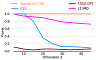
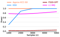
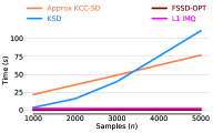
Figure 4: kcc-sd has more power than baseline methods with the imq kernel. Left: We compute $n=1000$ samples from $q=\prod_{i=1}^{d}\text{Laplace}(0,1/\sqrt{2})$ with target density $p=N(0,I_{d})$, and plot the power with increasing dimension. Middle and Right: Here we have samples from the same $p$ and $q$ distributions as before, but for fixed $d=30$ we increase the number of samples $n$ to show the number of samples required and computation time for baseline methods to achieve similar power as kcc-sd.

For the histogram-based sampler we use in our experiments, we use a two-layer neural network with $15$-dimensional hidden-layer with a sigmoid activation function. We train the model with gradient descent for $500$ epochs. We select the model with the lowest validation loss.

For fssd-opt we use $20\%$ of the samples for training and in approximate kcc-sd we use $20\%$ for training and $10\%$ for validation.

The $p$-value is computed as the proportion of the bootstrapped statistics, $R_{n}$, greater than the test statistic, $T_{n}$. And the power is computed as the proportion of $p$-values less than the significance level, in other words the power is the rejection rate of the null when the alternate hypothesis is true.

Choice of Kernel and Goodness-of-Fit tests.

All the experiments done with approximate kcc-sd, ksd and fssd-opt were done using the rbf kernel. The rbf kernel, a $C_{0}$ kernel (Definition 4.1, Carmeli et al. (2010)), suffices in defining consistent goodness-of-fit tests when comparing independent samples from a distribution $q$ (Theorem 2.2, Chwialkowski et al. (2016)).

Gorham and Mackey (2017) construct a sequence of empirical distributions, $q_{n}$, which does not converge to any distribution, a non-tight sequence. However, they prove that when comparing sequences $q_{n}$ with $p=N(\bm{0},I_{d})$ ksd with the rbf kernel still converges to zero. For this purpose they show that if ksd is computed with the imq kernel then ksd can enforce uniform tightness (Theorem 6, Gorham and Mackey (2017)).

However, as we have independent samples from a distribution $q$, this situation does not arise and we can use the rbf kernel. In Figure 4 we repeat the experiments from Figure 1 with imq kernel. In the left panel, we compare the power of the test using kcc-sd, r$\Phi$sd, ksd and fssd-opt with $q=\prod_{i=1}^{n}\text{Laplace}(0,1/\sqrt{2})$ and $p=N(\bm{0},I_{d})$. We compute $n=1000$ samples and then increase the dimension.

In the center and right panel of Figure 4, we compare the same distribution as above in $d=30$ with an increasing number of samples. We observe that kcc-sd requires less samples than the baseline methods to have power $1$, and for the baseline methods to have the same amount of power requires a similar amount of computation.

In the left panel of Figure 5, we have $p=N(\bm{0},\Sigma)$ with $\Sigma_{i,j}=0.5$ and $\Sigma_{i,i}=2$ and samples $\bm{x}_{i}=\bm{z}_{i}+\bm{\epsilon}_{i}$, where $\bm{\epsilon}_{i}\sim\prod_{j=1}^{d}\text{Laplace}(0,1/\sqrt{2})$ and $\bm{z}_{i}\sim N(\bm{0},\Sigma_{1})$ with ${(\Sigma_{1})}_{i,j}=0.5$ and ${(\Sigma_{1})}_{i,i}=1$, and $\bm{z}_{i}$ and $\bm{\epsilon}_{i}$ are independent. The samples from $q$ have the same mean and variance as $p$. We compute $n=500$ samples and increase the dimension. As the dimension increases, the power of the kcc-sd test with the imq kernels remains $1$, while the baseline methods with the imq kernels see a decline in power.

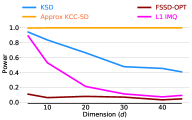
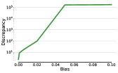
Figure 5: Left: Correlated Gaussian vs Correlated Gaussian with Laplace noise. As the dimension increases kcc-sd does not see a decrease in performance unlike the baseline methods. We use the imq kernel here. Right: As we add larger bias terms to the acceptance probability in the inner Metropolis sampler, samples from Metropolis-within-Gibbs sampler give larger kcc-sd.

Detecting Convergence of a Gibbs Sampler for Matrix Factorization.

Here we provide details of the probabilistic model considered in the experiments section for assessing the convergence of a Gibbs sampler for Bayesian probabilistic matrix factorization (Salakhutdinov and Mnih, 2008). We focus on a variant with two mean parameters $\mu_{V}$ and $\mu_{U}$ for user and movie feature vectors $U_{i}\in\mathbb{R}^{10},V_{j}\in\mathbb{R}^{10}$ and fixed the covariance matrix to the identity.

$$p(\bm{U}|\bm{\mu}_{U}) =\prod_{i=1}^{N}N(U_{i}|\bm{\mu}_{U},I),\quad p(\bm{\mu}_{U})=N(0,I)$$

$$p(\bm{V}|\bm{\mu}_{V}) =\prod_{j=1}^{M}N(V_{j}|\bm{\mu}_{V},I),\quad p(\bm{\mu}_{V})=N(0,I)$$

$$p(\bm{R}\mid\bm{U},\bm{V}) =\prod_{i=1}^{N}\prod_{j=1}^{M}{\left[N(R_{ij}\mid U_{i}^{T}V_{j},I)\right]}^{I_{ij}}$$

where $U_{i},V_{j}$ have normal priors and $I_{ij}$ is the indicator variable that is one if user $i$ rated movie $j$ and $0$ otherwise (see Appendix F).

Selecting Biased Samplers.

We use a simple bimodal Gaussian mixture model to demonstrate the power of kcc-sd in distinguishing biased samplers,

$$x_{i}\sim\frac{1}{2}N(\theta_{1},2)+\frac{1}{2}(\theta_{2},2)\ ,$$

where $\theta_{1},\theta_{2}$ have standard normal priors. We draw 100 samples of $x_{i}$ from the model with $(\theta_{1},\theta_{2})=(1,-1)$. We choose Metropolis-within-Gibbs to sample from the posterior over $\bm{\theta}$. This sampler uses a Metropolis sampler to sample each complete conditional inside the Gibbs sampler. We also use the Metropolis step to generate auxiliary variables used to calculate kcc-sd. Denote $q(\bm{\theta})$ to be the target distribution. The inner Metropolis step accepts the candidate $\bm{\theta}_{new}$ with probability $\min\left(1,q(\bm{\theta}_{new})/q(\bm{\theta}_{old})\right)$. Then we add a bias term to the acceptance probability, $\min\left(1,q(\bm{\theta}_{new})/q(\bm{\theta}_{old})+bias\right)$, thus the sampler is not unbiased anymore. We run for 60,000 iterations in total and drop the first 50,000 for burn-in. We show kcc-sds versus size of the bias terms in the right panel of Figure 5. kcc-sd increases with the size of the bias.

References

- Barbour (1990) Barbour, A. D. (1990). Stein’s method for diffusion approximations. Probability theory and related fields, 84(3):297–322.
- Barp et al. (2019) Barp, A., Briol, F.-X., Duncan, A., Girolami, M., and Mackey, L. (2019). Minimum stein discrepancy estimators. In Advances in Neural Information Processing Systems, pages 12964–12976.
- Carmeli et al. (2010) Carmeli, C., De Vito, E., Toigo, A., and Umanitá, V. (2010). Vector valued reproducing kernel hilbert spaces and universality. Analysis and Applications, 8(01):19–61.
- Chen et al. (2018) Chen, W. Y., Mackey, L., Gorham, J., Briol, F.-X., and Oates, C. J. (2018). Stein points. arXiv preprint arXiv:1803.10161.