Private Hierarchical Clustering and Efficient Approximation

Abstract.

In collaborative learning, multiple parties contribute their datasets to jointly deduce global machine learning models for numerous predictive tasks. Despite its efficacy, this learning paradigm fails to encompass critical application domains that involve highly sensitive data, such as healthcare and security analytics, where privacy risks limit entities to individually train models using only their own datasets. In this work, we target privacy-preserving collaborative hierarchical clustering. We introduce a formal security definition that aims to achieve balance between utility and privacy and present a two-party protocol that provably satisfies it. We then extend our protocol with: (i) an optimized version for single-linkage clustering, and (ii) scalable approximation variants. We implement all our schemes and experimentally evaluate their performance and accuracy on synthetic and real datasets, obtaining very encouraging results. For example, end-to-end execution of our secure approximate protocol for over $1$M $10$-dimensional data samples requires $35$sec of computation and achieves $97.09\%$ accuracy.

1. Introduction

Big-data analytics is an ubiquitous practice with a noticeable impact on our lives. Our digital interactions produce massive amounts of data that are analyzed in order to discover unknown patterns or correlations, which help us draw safer conclusions or make informed decisions. At the core of this lies Machine Learning (ML) for devising complex data models and predictive algorithms that provide hidden insights or automated actions, while optimizing certain objectives. Example applications that successfully employ ML are market forecast, service personalization, speech/face recognition, autonomous driving, health diagnostics and security analytics.

Of course, data analysis is only as good as the analyzed data, but this goes beyond the need to properly inspect, cleanse or transform high-fidelity data prior to its modeling: In most learning domains, analyzing “big data” is of twofold semantics: volume and variety.

First, the larger the dataset available to an ML algorithm, the better its learning accuracy, as irregularities due to outliers fade away faster. Indeed, scalability to large dataset sizes is very important, especially so in unsupervised learning, where model inference uses unlabelled observations (evading points of saturation, encountered in supervised learning, where new training sets improve accuracy only marginally). Also, the more varied the collected data, the more elaborate its analysis, as degradation due to noise reduces and domain coverage increases. Indeed, for a given learning objective, say classification or anomaly detection, combining more datasets of similar type but different origin enables discovery of more complex, interesting, hidden structures and of richer association rules (correlation or causality) among attributes. So, ML models improve their predictive power when they are built over multiple datasets owned and contributed by different entities, in what is termed collaborative learning—and widely considered as the golden standard (Stoica et al., 2017).

Privacy-preserving hierarchical clustering. Several learning tasks of interest, across a variety of application domains, such as healthcare or security analytics, demand deriving accurate ML models over highly sensitive data—e.g., personal, proprietary, customer, or other types of data that induce liability risks. By default, since collaborative learning inherently implies some form of data sharing, entities in possession of such confidential datasets are left with no other option than simply running their own local models, severely impacting the efficacy of the learning task at hand. Thus, privacy risks are the main impediment to collaboratively learning richer models over large volumes of varied, individually contributed, data.

The security and ML community has embraced the concept of Privacy-preserving Collaborative Learning (PCL), the premise being that effective analytics over sensitive data is feasible by building global models in ways that protect privacy. This is closely related to (privacy-preserving) ML-as-a-Service (Hesamifard et al., 2018; Gilad-Bachrach et al., 2016; Tanuwidjaja et al., 2020; Hesamifard et al., 2017) that utilizes cloud providers for ML tasks, without parties revealing their sensitive raw data (e.g., using encrypted or sanitized data. Existing work on PCL mostly focuses on supervised rather than unsupervised learning tasks (with a few exceptions such as $k$-means clustering). As unsupervised learning is a prevalent paradigm, the design of ML protocols that promote collaboration and privacy is vital.

In this paper, we study the problem of privacy-preserving hierarchical clustering. This unsupervised learning method groups data points into similarity clusters, using some well-defined distance metric. The “hierarchic” part is because each data point starts as a separate “singleton” cluster and clusters are iteratively merged building increasingly larger clusters. This process forms a natural hierarchy of clusters that is part of the output, showing how the final clustering was produced. We present scalable cryptographic protocols that allow two parties to privately learn a model for the joint clusters of their combined datasets. Importantly, we propose a formal security definition for this task in the MPC framework and prove our protocols satisfy it. In contrast, prior works for privacy-preserving hierarchical clustering have proposed crypto-assisted protocols but without offering rigorous security definitions or analysis (e.g., (Inan et al., 2007; De and Tripathy, 2014; Jagannathan et al., 2010); see detailed discussion in Section 8).

Motivating applications. Hierarchical clustering is a class of unsupervised learning methods that build a hierarchy of clusters over an input dataset, typically in bottom-up fashion. Clusters are initialized to each contain a single input point and are iteratively merged in pairs, according to a linkage metric that measures clusters’ closeness based on their contained points. Here, unlike other clustering methods ($k$-means or spectral clustering), different distance metrics can define cluster linkage (e.g., nearest neighbor and diameter for single and complete linkage, respectively) and flexible conditions on these metrics can determine when merging ends. The final output is a dendrogram with all formed clusters and their merging history. This richer clustering type is widely used in practice, often in areas where the need for scalable PCL solutions is profound.

In healthcare, for instance, hierarchical clustering allows researchers, clinicians and policy makers to process medical data and discover useful correlations to improve health practices—e.g., discover similar genes types (Eisen et al., 1998), patient profiles most in need of targeted intervention (Weir et al., 2000; Newcomer et al., 2011) or changes in healthcare costs for specific treatments (Liao et al., 2016). To be of any predictive value, such data contains sensitive information (e.g., patient records, gene information, or PII) that must be protected, also due to legislations such as HIPPA in US or GDPR in EU. Also, in security analytics, hierarchical clustering allows enterprise security personnel to process log data on network/users activity to discover suspicious or malicious events—e.g., detect botnets (Gu et al., 2008), malicious traffic (Nelms et al., 2013), compromised accounts (Cao et al., 2014), or malware (Bayer et al., 2009). Again, such data contains sensitive information (e.g., employee/customer data, enterprise security posture, defense practices, etc.) that must be protected, also due to industrial regulations or for reduced liability. As such, without privacy provisions for joint cluster analysis, entities are restricted to learn only local clusters, thus confined in accuracy and effectiveness. E.g., a clinical-trial analysis over patients of one hospital may introduce bias on geographic population, or network inspection of one enterprise may miss crucial insight from attacks against others.

In contrast, our treatment of clustering as a PCL instance is a solid step towards richer classification. Our protocols for private hierarchical clustering incentivize entities to contribute their private datasets for joint cluster analysis over larger and more varied data collections, to get in return more refined results. For instance, hospitals can jointly cluster medical data extracted from their combined patient records, to provide better treatment, and enterprises can jointly cluster threat indicators collected from their combined SIEM tools, to present timely and stronger defenses against attacks. At all times, data owners protect the confidentiality of their private data and remain compliant with current regulations.

Challenges and insights. A first challenge we faced is how to rigorously specify the secure functionality that such protocols must achieve. A secure protocol guarantees that no party learns anything about the input of the other party, except what can be inferred after parties learn the output. But since the output dendrogram of hierarchical clustering already includes the (now partitioned) input, this problem cannot directly benefit from MPC. This issue is partially the reason why previous approaches for hierarchical clustering (see discussion in Section 8 and an excellent survey of related work by Hegde et al. (Hegde et al., 2021)) lack formal security analysis or have significant information leakage. To overcome this, our approach is to modify and refine what private hierarchical clustering should produce, redacting the joint output—sufficiently enough, to allow the needed input privacy protection, but minimally so, to preserve the learning utility. We introduce a security notion that is based on point-agnostic dendrograms, which explicitly capture only the merging history of formed joint clusters and useful statistics thereof, to balance the intended accuracy against the achieved privacy. To the best of our knowledge, our formal security definition (Section 3) is the first such attempt for the case of hierarchical clustering.

The next challenge is to securely realize this functionality efficiently. Standard tools for secure two-party computation, e.g., garbled circuits (Yao, 1982, 1986), result in large communication, while fully homomorphic encryption (Gentry, 2009) is still rather impractical, so designing scalable hierarchical clustering PCL protocols is challenging. Moreover, hierarchical clustering of $n$ points is already computation-heavy—of $\mathcal{O}(n^{3})$ cost. As such, approximation algorithms, e.g., CURE (Guha et al., 2001), are the de facto means to scale to massive datasets, but incorporating approximation to private computation is not trivial—as complications often arise in defining security (Feigenbaum et al., 2006).

In Section 4, we follow a modular design approach and use cryptography judiciously by devising our main construction as a mixed protocol (e.g., (Henecka et al., 1999; Demmler et al., 2015; Kerschbaum et al., 2014)). We decompose our refined hierarchical clustering into building blocks and then we select a combination of tools that achieves fast computation and low bandwidth usage. In particular, we conveniently use garbled circuits for cluster merging, but additive homomorphic encryption (Paillier, 1999) for cluster encoding, while securely “connecting” the two steps’ outputs.

In Section 5, we evaluate the performance and security of our main protocol and present an optimized variant of $O(n^{2})$ cost for single linkage. In Section 6, we integrate the CURE method (Guha et al., 2001) for approximate clustering into our design, to get the best-of-two-worlds quality of high scalability and privacy. We study different secure approximate variants that exhibit trade-offs between efficiency and accuracy without extra leakage due to approximation. In Section 7, we report results from the experimental evaluation of our protocols on synthetic and real data that confirm their practicality. For example, end-to-end execution of our private approximate single-linkage protocol for $1$M $10-d$ records, achieves $97.09\%$ accuracy at very with only $35$sec of computation time.

Summary of contributions. Overall, in this work our results can be summarized as follows:

• We provide a formal definition and secure two-party protocols for private hierarchical clustering for single or complete linkage.

• We present an optimized protocol for single linkage that significantly improves the computational and communication costs.

• We combine approximate clustering methods with our protocols to get variants that achieve both scalability and strong privacy.

• We experimentally evaluate the performance of our protocols via a prototype implementation over synthetic and real datasets.

2. Preliminaries

Hierarchical clustering (HC). For fixed positive integers $d,l$, let $\mathcal{D}=\{v_{i}|v_{i}\in\mathbb{Z}_{2^{l}}^{d}\}_{i=1}^{n}$ be an unlabeled indexed dataset of $n$ $d$-dimensional points, where w.l.o.g, we set the domain to $\{0,\ldots,2^{l}-1\}$. Over pairs $x,y\in\mathcal{D}$ of points, point distance is measured using the standard square Euclidean distance metric ${\mathsf{dist}}(x,y)=\sum_{j=1}^{d}(x_{j}-y_{j})^{2}$. Over pairs $X,Y\subseteq\mathcal{D}$ of sets of points, set closeness is measured using a linkage distance metric $\delta(X,Y)$, as a function of the cross-set distances of points contained in $X$, $Y$. The most commonly used linkage distances are the single linkage (or nearest neighbor) defined as $\delta(X,Y)={\mathsf{min}}_{x\in X,y\in Y}{\mathsf{dist}}(x,y)$, and the complete linkage (or diameter) defined as $\delta(X,Y)={\mathsf{max}}_{x\in X,y\in Y}{\mathsf{dist}}(x,y)$.

Standard agglomerative HC methods use set closeness to form clusters in a bottom-up fashion, as described in algorithm $\mathsf{HCAlg}$ (Figure 1). It receives an $n$-point dataset $\mathcal{D}$ and groups its points into a total of $\ell_{t}\leq n$ target clusters, by iteratively merging pairs of closest clusters into their union. The merging history is stored (redundantly) in a dendrogram $T$, that is, a forest of clusters of $n-\ell_{t}+1$ levels, where siblings correspond to merged clusters and levels to dataset partitions, build level-by-level as follows:

• Initially, each input point $v_{i}\in\mathcal{D}$ forms a singleton cluster $\{v_{i}\}$ as a leaf in $T$ (at its lowest level $n$).

• Iteratively, in $n-\ell_{t}$ clustering rounds, the $i$ root clusters (at top level $i$) form $i-1$ new root clusters in $T$ (at higher level $i-1$), with the closest two merged into a union cluster as their parent, and each other cluster copied to level $i-1$ as its parent.

When a new level of $\ell_{t}$ target clusters is reached, $\mathsf{HCAlg}$ halts and outputs $T$. The exact value of $\ell_{t}\in[1:n]$ is determined during execution via a predefined condition $\mathsf{End}$ checked over the current state $T$ and a termination parameter $t$ provided as additional input. This allows for flexible termination conditions—e.g., stopping when inter-cluster distance drops below an threshold specified by $t$, or simply when exactly $\ell_{t}=t$ target clusters are formed.

Typically, the dendrogram $T$ is augmented to store some associated cluster metadata, by keeping, after any union/copy cluster is formed, some useful statistics over its contained points. Common such statistics for cluster $C$ is its size $size(C)=|C|$ and representative value $rep(C)$, usually defined as its centroid (i.e., a certain type of average) point. Overall, for a set $M$ of cluster statistics of interest and specified linkage distance and termination condition, $\mathsf{HCAlg}$ is viewed to operate on indexed dataset $\mathcal{D}=\{v_{i}\}_{i=1}^{n}$ and return an $M$-augmented dendrogram $T$, comprised of: (1) the forest structure of dendrogram $T$, specifying the full merging history of input points into formed clusters (from $n$ singletons to $\ell_{t}$ target ones); (2) the cluster set $C(T)$; and (3) the metadata set $M(T)$ associated with (clusters in) $T$. Assuming that $\mathsf{HCAlg}$ employs a fixed tie-breaking method in merging clusters, its execution is deterministic.

Hierarchical Clustering Algorithm $\mathsf{HCAlg}$ Input: Indexed set $\mathcal{D}=\{{\bf v}_{i}\}_{i=1}^{n}$, termination parameter $t$ Output: Dendrogram $T$, clusters $C(T)$, metadata $M(T)$ Parameters: Linkage distance $\delta(\cdot,\cdot)$, termination condition $\mathsf{End}(\cdot,\cdot)$, cluster statistics set $M\supseteq\{rep(\cdot),size(\cdot)\}$ [Initially, at level $n$] 1. Initialize dendrogram $T$: For each $i=1,\ldots,n$: – Create node $u_{i}$ as the $i$th left-most leaf in $T$. – Set $C(u_{i})=\{{\bf v}_{i}\}$ as the singleton cluster of $u_{i}$. – Compute $M(u_{i})=\{m({\bf v}_{i})|m\in M\}$ as statistics of $u_{i}$. 2. Set up linkages: Compute linkages of all pairs of singleton clusters as a dictionary $D$, where $\{C(u_{i}),C(u_{j})\}$ is keyed under $\delta(C(u_{i}),C(u_{j}))$, $1\leq i<j\leq n$. [Iteratively, at level $i=n,\ldots,\ell_{t}+1$] 1. Update $T$: If $N_{i}$ is the set of nodes in $T$ at level $i$: – Find in $D$ the min-linkage pair $(u,u^{\prime})$ of nodes in $N_{i}$, breaking ties using a fixed rule over leaf-node indices. – Create node $w\in N_{i-1}$ as parent of $u$ and $u^{\prime}$; set $C(w)=C(u)\cup C(u^{\prime})$; for each node $\bar{u}\in N_{i}-\{u,u^{\prime}\}$, create node $\bar{w}\in N_{i-1}$ as parent of $\bar{u}$; set $C(\bar{w})=C(\bar{u})$. – For each node $\hat{w}\in N_{i-1}$, compute $M(\hat{w})$. 2. Check termination: If $\mathsf{End}(T,t)==1$, terminate. 3. Update linkages: Compute linkage $\delta(C(w),C(\bar{w}))$, for all $\bar{w}\in N_{i-1}-\{w\}$, and consistently update dictionary $D$.

Figure 1. Agglomerative hierarchical clustering.

Secure computation and threat model. We consider the standard setting for private two-party computation, where two parties wishing to evaluate function $f(\cdot,\cdot)$ on their individual, private inputs $x_{1}$, $x_{2}$, engage in an interactive cryptographic protocol that upon termination returns to them the common output $y=f(x_{1},x_{2})$. Protocol security has this semantics: Subject to certain computational assumptions and misbehavior types during protocol execution, no party learns anything about the input of the other party, other than what can be inferred by its own input $x_{i}$ and the learned result $y$. In this context, we study privacy-preserving hierarchical clustering in the semi-honest adversarial model which assumes that parties are honest, but curious: They will follow the prescribed protocol but also seek to infer information about the input of the other party, by examining the transcript of exchanged messages—the latter, assumed to be transferred over a reliable channel.

Although, in practice, parties may choose to be malicious, deviating from the prescribed protocol if they can benefit from this and can avoid detection, the semi-honest adversarial model still has its merits, especially in the studied PCL setting. Namely, it provides essential privacy protection for any privacy-aware party to enter the joint computation to benefit from collaborative learning. We note that, by trading off efficiency, security can be hardened via known generic techniques for compiling protocols secure in this model into counterparts secure against malicious parties.

Garbled circuits. One of the most widely used tools for two-party secure computation, Garbled Circuits (GC) (Yao, 1982, 1986) allow two parties to evaluate a boolean circuit on their joint data without revealing their respective inputs. This is done by generating an encrypted truth table for each gate while evaluating the circuit by decrypting these tables in a way that preserves input privacy. In Appendix A, we provide more details about the GC framework.

Homomorphic encryption. This technique allows carrying out operations over encrypted data. Fully Homomorphic Encryption (FHE) (Gentry, 2009) can evaluate arbitrary functions over ciphertexts, but remains rather impractical. Partially homomorphic encryption supports only specific arithmetic operations over ciphertexts, but allows for very efficient implementations (Rivest et al., 1978; Paillier, 1999). We use Paillier’s scheme for Additively Homomorphic Encryption (AHE) (Paillier, 1999), summarized as follows. For security parameter $\lambda$, keys generated by running $({\sf pk},{\sf sk})\leftarrow{\mathsf{Gen}}(1^{\lambda})$ and a public RSA modulus $N$, the scheme encrypts (with public key ${\sf pk}$) any message $m$ in the plaintext space $\mathbb{Z}_{N}$ into a ciphertext $[m]$, ensuring that decryption (with secret key $sk$) of any ciphertext product $[m]\cdot[m^{\prime}]\mod N^{2}$ (computable without ${\sf sk}$) results in the plaintext sum $m+m^{\prime}\mod N$. Thus, decrypting $[m]^{k}\mod N^{2}$ results in $km\mod N$, and the ciphertext product $[m]\cdot[0]$ results in a fresh encryption of $m$.

3. Formal Problem Specification

We introduce a model for studying private hierarchical clustering, the first to provide formal specifications for secure two-party protocols for this central PCL problem. Importantly, we define security for a refined learning task that achieves a meaningful balance between the intended accuracy and privacy—a necessary compromise for the problem at hand to even be defined as a PCL instance!

We first formulate two-party privacy-preserving hierarchical clustering as a secure computation. Parties ${\mathsf{P_{1}}}$, ${\mathsf{P_{2}}}$ hold independently owned datasets $P$, $Q$ of points in $\mathbb{Z}_{2^{l}}^{d}$, and wish to perform a collaborative hierarchical clustering over the combined set $\mathcal{D}=P\cup Q$. They agree on the exact specification $f_{HC}$ of this learning task, as a function of their individually contributed datasets that encompasses all other parameters (e.g., for termination).

Let $\Pi$ be a two-party protocol that correctly realizes $f_{HC}(\cdot,\cdot)$: Run jointly on inputs $x_{1}$, $x_{2}$, $\Pi$ returns the common output $f_{HC}(x_{1},x_{2})$. Thus, parties ${\mathsf{P_{1}}}$, ${\mathsf{P_{2}}}$ can learn cluster model $f_{HC}(P,Q)$ by running protocol $\Pi$ on their inputs $P$, $Q$. As discussed, $\Pi$ is considered to be secure if its execution prevents an honest-but-curious party from learning anything about the other party’s input that is not implied by the learned output. We formalize this intuitive privacy requirement via the standard two-party ideal/real world paradigm (Goldreich et al., 1987).

Ideal functionality. First, we define what one can best hope for. Cluster analysis with perfect privacy is trivial in an ideal world, where ${\mathsf{P_{1}}}$, ${\mathsf{P_{2}}}$ instantly hand-in their inputs $x_{1}$, $x_{2}$ to a trusted third party, called the ideal functionality $f_{HC}$, that computes and announces $f_{HC}(x_{1},x_{2})$ (and explodes). Here, the use of terms “perfect” and “ideal” is fully justified for no information about any private input is leaked during the computation. Some information about $x_{1}$ or $x_{2}$ may be inferred after the output is announced, by combining the known $x_{2}$ or $x_{1}$ with the learned $f_{HC}(x_{1},x_{2})$: It is the inherent price for collaboratively learning a non-trivial function.

In the real world, ${\mathsf{P_{1}}}$, ${\mathsf{P_{2}}}$ learn $f_{HC}(x_{1},x_{2})$ by interacting in the joint execution of a protocol $\Pi$. We measure the privacy quality of $\Pi$ against the ideal-world perfect privacy, dictating that running $\Pi$ is effectively equivalent to calling the ideal functionality $f_{HC}$. Informally, $\Pi$ securely realizes $f_{HC}$, if anything computable by an efficient semi-honest party ${\mathsf{P_{i}}}$ in the real world, can be simulated by an efficient algorithm (called the simulator $\mathsf{Sim}$), acting as ${\mathsf{P_{i}}}$ in the ideal world; i.e., $\Pi$ leaks no information about a private input during execution, subject to the price for learning $f_{HC}(x_{1},x_{2})$.

Next comes the question of which ideal functionality $f_{HC}$ should $\Pi$ securely realize for private joint hierarchical clustering? Though tempting, equating $f_{HC}$ with the legacy algorithm $\mathsf{HCAlg}$ (Figure 1), thus learning a full-form augmented dendrogram, slides us into a degeneracy. Assume $f_{HC}$ merely runs $\mathsf{HCAlg}$ on the combined indexed set $\mathcal{D}=P\cup Q=\{d_{k}\}_{k=1}^{n}$, $n=|P|+|Q|$. The learned model is the dendrogram $T$ along with its associated clusters $C(T)$ and metadata $M(T)$. But set $C(T)$ itself reveals the input $\mathcal{D}$; in this case, the price for collaborative learning is full disclosure of sensitive data and nothing is to be protected! This raises the question of limiting exactly what information about $P,Q$ should be revealed by $f_{HC}$ which is the focus of the remainder of this section.

Ideal Functionality $f_{HC}^{*}(\cdot,\cdot)$ Input: Sets $P=\{p_{i}\}_{1}^{n_{1}}$, $Q=\{q_{j}\}_{1}^{n_{2}}$ Output: Dendrogram $T^{*}$, metadata $M^{*}\supseteq\{rep(\cdot),size(\cdot)\}$ Parameters: Linkage distance $\delta(\cdot,\cdot)$, termination condition $\mathsf{End}(\cdot,t)$, cluster statistics set $M$, selection function $\mathsf{S(\cdot)}$ [Pre-process] Form input of size $n=n_{1}+n_{2}$ for $\mathsf{HCAlg}$: 1. Set $\mathcal{D}=\{d_{k}\}_{1}^{n}$ s.t. $d_{k}=p_{k}$, if $k\leq n_{1}$, or else $d_{k}=q_{k-n_{1}}$. 2. Pick random permutation $\pi:[n]\rightarrow[n]$; set $\mathcal{D}^{*}=\pi(\mathcal{D})$. [HC-process] Run $\mathsf{HCAlg}(\mathcal{D}^{*},t)$ w/ parameters $\delta$, $M$, $\mathsf{End}$. [Post-process] Redact output $T^{*}$, $C(T^{*})$, $M(T^{*})$ of $\mathsf{HCAlg}$: 1. Set $M^{*}=\emptyset$; $\forall v\in T^{*}$: if $\mathsf{S}(v)==1$, $M^{*}\leftarrow M^{*}\cup\{M(v)\}$. 2. Return $T^{*}$, $M^{*}$.

Figure 2. Ideal functionality $f_{HC}^{*}$ for hierarchical clustering.

Refined cluster analysis. In the PCL setting, we need a new definition of hierarchical clustering that distills the full augmented dendrogram $\{T,C(T),M(T)\}$ into a redacted, but still useful, learned model, balancing between accuracy (to benefit from clustering) and privacy (to allow collaboration). If allowing the ideal functionality $f_{HC}$ to return $C(T)$ is one extreme that diminishes privacy, removing the dendrogram $T$ from the output—to learn only about its associated information $C(T)$, $M(T)$—is another that diminishes accuracy. Indeed, if $T$, which captures the full merging history in its structure, is excluded from the output of $f_{HC}$, a core feature in HC is lost: the ability to gain insights on how target clusters were formed, under what hierarchies and in which order. This renders the HC analysis only as good as much simpler techniques (e.g., $k$-means) that merely discover pure similarity statistics of target clusters. As the motivation for studying collaborative HC as a prominent and widely used unsupervised learning task, in the first place, lies exactly on its ability to discover such rich inter-cluster relations, we must keep the forest structure of $T$ in $f_{HC}$’s output.

Avoiding the above two degenerate extremes suggests that the learned model $f_{HC}(P,Q)$ should necessarily include the cluster hierarchy $T$ but not the clusters $C(T)$ themselves. Yet, the obvious middle-point approach of learning model $f^{m}_{HC}(P,Q)=\{T,M(T)\}$ remains suboptimal in terms of privacy protections, as the learned output can still be strongly correlated to exact input points. Indeed, given $T$ and a party’s own input, inferring points of the other party’s input simply amounts to identifying singleton clusters, which is generally possible by inspecting and correlating the (hard-coded in $\mathsf{HCAlg}$) indices in $\mathcal{D}$ with the metadata associated to singletons (or their close neighbors). For instance, if $w$ is the parent of singleton $u$ and cluster $u^{\prime}$ in $T$, then ${\mathsf{P_{1}}}$ can infer input point $C(u)$ of ${\mathsf{P_{2}}}$, either directly from output $M(u)$, if $u$ is known to store none of its input points, or indirectly from $M(u^{\prime})$, $M(w)$, if these output values imply a value of $M(u)$ that is consistent with none of its own inputs.

Also, even without singleton clusters in the output, there is still leakage from the positioning of the points at the leaf level of $T$. E.g., assuming $P,Q$ are ordered from left to right, a merging of two points at the right half of the tree during the first merge reveals to ${\mathsf{P_{1}}}$ that ${\mathsf{P_{2}}}$ has a pair of points with smaller distance than the minimum distance observed among points in $P$. Hence, it is crucial to eliminate information about the positioning of clusters in $T$.

Point-agnostic dendrogram. Such considerations naturally lead to a new goal: We seek to refine further, but minimally so, the middle-point model $f^{m}_{HC}(P,Q)=\{T,M(T)\}$ into an optimized model $f^{*}_{HC}(P,Q)=\{T^{*},M^{*}(T)\}$, whereby no private input points directly leak to any of the parties, after the output is announced. This quality is well-defined, intuitive and useful: Unless the intended joint hierarchical clustering explicitly copies some of input points to the output, the learned model $f^{*}_{HC}(P,Q)$ should allow no party to explicitly learn, that is, to deterministically deduce with certainty, any of the unknown input points of the other party.

We accordingly set our ideal functionality $f^{*}_{HC}$ for hierarchical clustering to outputs a point-agnostic augmented dendrogram, defined by merely running algorithm $\mathsf{HCAlg}$, subject to a twofold correction of its input $P$, $Q$ and returned dendrogram (Figure 2):

• Pre-process input: Run $\mathsf{HCAlg}$ on indexed set $\mathcal{D}^{*}$ that is a random permutation over the combined set $\mathcal{D}=P\cup Q=\{d_{k}\}_{k=1}^{n}$.

• Post-process output: Return the output $T^{*}$, $C(T^{*})$, $M(T^{*})$ of $\mathsf{HCAlg}$ redacted as $T^{*},M^{*}(T^{*})\subset M(T^{*})$, including metadata of only a few safe clusters in $T^{*}$.

Our ideal functionality $f^{*}_{HC}$ refines the ordinary dendrogram $T$, $C(T)$, $M(T)$: Running $\mathsf{HCAlg}$ on the randomly permuted input $\mathcal{D}^{*}$ (instead of $\mathcal{D}$) results in a new randomized forest structure $T^{*}$ (instead of $T$) and, although its associated sets of formed clusters $C(T^{*})$ and metadata $M(T^{*})$ remain the same, the learned model includes no elements from $C(T^{*})$, but only specific elements from $M(T^{*})$, determined by a selection function $\mathsf{S}(\cdot)$ (as a parameter agreed upon among the parties and hard-coded in $f^{*}_{HC}$). Such metadata is safe to learn, in the sense that it does not directly leak any input points.

We propose the following two orthogonal strategies for safe metadata selection for point-agnostic dendrograms:

• $s$-Merging selection: $M(w)\in M(T^{*})$ if $w$ is the parent of $u$, $u^{\prime}$ in $T^{*}$ and $|C(u)|,|C(u^{\prime})|>s$: any non-singleton cluster formed by merging two clusters of size above threshold $s>0$, is safe;

• Target selection: $M(w)\in M(T^{*})$ if $w$ is root in $T^{*}$: any target cluster at level $\ell_{t}$ in $T^{*}$ is safe.

Above, the first strategy ensures that no direct leakage of private input points occurs by correlating statistics of thin neighboring clusters; in particular, no cluster statistics are learned for singletons or their parents ($s=1$), thus eliminating the type of leakage allowed by model $f^{m}_{HC}(P,Q)$. The second strategy ensures that only statistics of target clusters are learned, that is, input points may be directly learned only explicitly as part of the intended cluster analysis.

Overall, the resulting dendrogram is point-agnostic in the sense that neither the forest structure of $T^{*}$ nor the metadata $M(T^{*})$ reveal which singletons a party’s points are mapped to. As points are randomly mapped to singletons, ties in cluster merging are randomly broken, and no statistics are learned for singleton (or thin) clusters, no party can deduce with certainty any of the other party’s input points. For instance, the applied permutation eliminates leakage from the positioning of the singleton cluster at the leaves that, in our previous example, allowed one to infer whether the other party owned points with smaller distance than its own pairs, from the first-round clustering result. More generally, anything inferable about a party’s private input relates to a meta-analysis that must necessarily encompass the (unknown) input distribution and the random permutation used by $f^{*}_{HC}$. This can be viewed as an inherent price of collaborative hierarchical clustering. The following defines the security of privacy-preserving hierarchical clustering.

Definition 3.1.

A two-party protocol $\Pi$, jointly run by ${\mathsf{P_{1}}}$, ${\mathsf{P_{2}}}$ on respective inputs $x_{1}$, $x_{2}$ using individual random tapes $r_{1}$, $r_{2}$ that result in incoming-message transcripts $t_{1}$, $t_{2}$, is said to be secure for collaborative privacy-preserving hierarchical clustering in the presence of static, semi-honest adversaries, if it securely realizes the ideal functionality $f^{*}_{HC}$ defined in Figure 2, by satisfying the following: For $i=1,2$ and for any security parameter $\lambda$, there exists a non-uniform probabilistic polynomial-time simulator $\mathsf{Sim}_{{\mathsf{P_{i}}}}$ so that $\mathsf{Sim}_{{\mathsf{P_{i}}}}(1^{\lambda},x_{i},f^{*}_{HC}(x_{1},x_{2}))\cong\mathsf{view}_{\mathcal{A}^{\Pi}_{{\mathsf{P_{i}}}}}\triangleq\{r_{i},t_{i}\}$.

4. Main Construction

We now present our main construction, protocol ${\mathsf{PHC}}$ for Private Hieararchical Clustering that securely realizes the ideal functionality $f^{*}_{HC}$ (of Figure 2) when jointly run by parties ${\mathsf{P_{1}}},{\mathsf{P_{2}}}$.

General approach. As discussed earlier, for efficiency reasons, we seek to avoid carrying out hierarchical clustering—a complex and inherently iterative process of cubic costs—in its entirety by computing over ciphertext (e.g., via GC or FHE). Instead, we adopt a mixed-protocols design, decomposing hierarchical clustering into more elementary tasks. We then use tailored secure and efficient protocols for each task, and combine these components into a final protocol, in ways that minimize the cost in converting data encoding between individual sub-protocols. Hence, our solution is a secure mixed-protocol specifically tailored for hierarchical clustering.

It is worth noting that generic solutions from 2-party computation (2PC) (e.g., (Demmler et al., 2015)), would solve the problem but would not easily scale to large datasets. During hierarchical clustering, we need to maintain a distance matrix between two parties with space complexity $O(n^{2})$. If one relies solely on a single generic approach such as GC or secret sharing, the communication bandwidth would become the bottleneck. Hence, using additively homomorphic encryption during our protocol’s setup phase in order to produce a “shared permuted” distance matrix allows us not only to hide the correspondence between euclidean distances and original points, but also to be more communication efficient eventually. Another advantage compared to other 2PC techniques is that our approach can achieve better precision as we explain in more detail in Section 7.

Our protocol securely implements $f^{*}_{HC}$ for the configuration that the parties specify: linkage $\delta(\cdot,\cdot)$, termination condition $\mathsf{End}(\cdot,t)$, cluster statistics set $M$, selection function $\mathsf{S(\cdot)}$. Yet for simplicity, hereby, we use the following default configurations, where:

1. complete linkage over one-dimensional data is used;

2. the termination condition results in $t$ target nodes;

3. target selection is used for safe metadata selection; and

4. only representative values and size statistics are learned.

That is, by (2) - (4) in what follows (and in our experiments in Section 7), the set of redacted statistics $M^{*}$ consists of the representatives $rep_{1},\ldots,rep_{\ell_{t}}$ and sizes $size_{1},\ldots,size_{\ell_{t}}$ of $\ell_{t}=t$ target clusters (recall that representatives are a predefined type of centroid of the cluster, e.g., average or median), where $t$ is fixed in advance. Configuration 1) is used only for clarity; we discuss optimizations for single linkage and extensions to higher dimensions in Section 5 (and we report on the evaluation of such extensions in Section 7).

${\mathsf{P_{1}}}$’s Input: $P=\{p_{1},\dots,p_{n_{1}}\}$, security parameter $\lambda$

${\mathsf{P_{2}}}$’s Input: $Q=\{q_{1},\dots,q_{n_{2}}\}$, security parameter $\lambda$

Output: Merging history, $\{rep(\cdot)$, $size(\cdot)\}$ of $t$ target nodes

Parameters: Default configurations

1 ${\mathsf{P_{1}}}$: Generate $({\sf pk},{\sf sk})\leftarrow{\mathsf{Gen}}(1^{\lambda})$; send ${\sf pk}$ to ${\mathsf{P_{2}}}$

2${\mathsf{P_{2}}}$: Generate $({\sf pk}^{\prime},{\sf sk}^{\prime})\leftarrow{\mathsf{Gen}}(1^{\lambda})$; send ${\sf pk}^{\prime}$ to ${\mathsf{P_{1}}}$

3${\mathsf{P_{1}}},{\mathsf{P_{2}}}$: Jointly run ${\mathsf{PHC}}.{\mathsf{Setup}}$, ${\mathsf{PHC}}.{\mathsf{Cluster}}$, ${\mathsf{PHC}}.{\mathsf{Output}}$

Algorithm 1 ${\mathsf{PHC}}$: Private Cluster Analysis

Protocol overview. After choosing configurations, ${\mathsf{P_{1}}},{\mathsf{P_{2}}}$ run protocol ${\mathsf{PHC}}$ (Algorithm 1), with inputs their datasets $P,Q$ of $n_{1},n_{2}$ points, $n=n_{1}+n_{2}$, security parameter $\lambda$, and statistical parameter $\kappa$. Each party establishes its individual Paillier key-pair, and then parties exchange their corresponding public keys.

Then, parties run sub-protocols ${\mathsf{PHC}}.{\mathsf{Setup}}$, ${\mathsf{PHC}}.{\mathsf{Cluster}}$ and ${\mathsf{PHC}}.{\mathsf{Output}}$, which comprise the three main phases in our protocol, in direct analogy to the three components of $f^{*}_{HC}$. The general flow of our protocol is described below, in reference to also Figure 3.

In a setup phase, sub-protocol ${\mathsf{PHC}}.{\mathsf{Setup}}$ processes the $n$ input points, viewed as an input array $I$, and all pairwise distances among these points, viewed as a $n\times n$ cluster distance matrix $\Delta$. Here, $I,\Delta$ are only virtual, corresponding to an early joint state of ${\mathsf{P_{1}}},{\mathsf{P_{2}}}$ that is actually secret-shared between them. Specifically, ${\mathsf{P_{1}}}$ holds an array $L$ with exactly $I$’s elements but each AHE-encrypted under ${\mathsf{P_{2}}}$’s secret key, and a $n\times n$ matrix $R$ with random blinding terms, whereas ${\mathsf{P_{2}}}$ holds the matrix $B=\Delta+R$ with blinded pairwise cluster distances. Importantly, as $f^{*}_{HC}$ specifies, the joint state $\{I,\Delta\}$ is split only after $I$’s elements and $\Delta$’s rows and columns are randomly shuffled, with ${\mathsf{P_{1}}},{\mathsf{P_{2}}}$ not knowing the exact shuffling used.

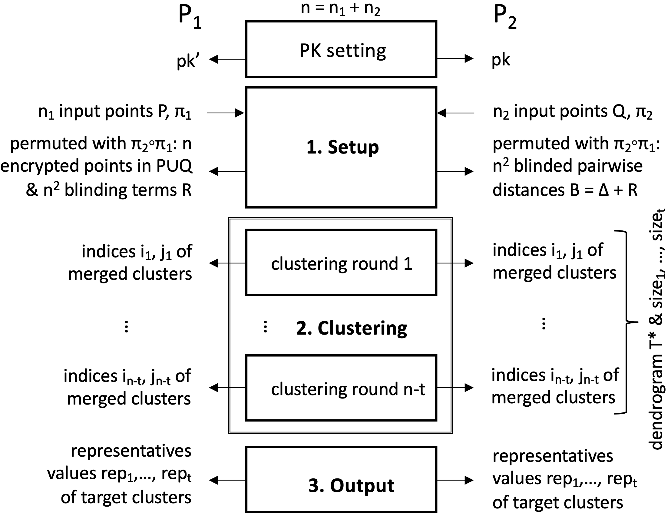
Figure 3. Overall workflow of our protocol ${\mathsf{PHC}}$.

In a clustering phase, sub-protocol ${\mathsf{PHC}}.{\mathsf{Cluster}}$ virtually runs the ordinary hierarchical clustering algorithm $\mathsf{HCAlg}$ on matrix $\Delta$: ${\mathsf{P_{1}}},{\mathsf{P_{2}}}$ process their individual states $R,B$ to iteratively merge singletons into target clusters, based on inter-cluster distances in $\Delta$. Each iteration merges two clusters into a new one via three tasks:

• Find pair: First, ${\mathsf{P_{1}}},{\mathsf{P_{2}}}$ find the closest-cluster pair $(i,j)=\mathsf{argMin}(\Delta)$, $i<j$, to merge, i.e., the indices in $\Delta$ of the minimum inter-cluster distance $D_{ij}$.

• Update linkages: Then, ${\mathsf{P_{1}}},{\mathsf{P_{2}}}$ update $\Delta$ to $\Delta^{\prime}=B^{\prime}-R^{\prime}$ with the new cluster distances after pair $(i,j)$ is merged into cluster $C=C_{i}\cup C_{j}$. This entails computing (and splitting via a fresh blinding term) distance $\delta(C,C^{\prime})$ between $C$ and each not-merged cluster $C^{\prime}$, which equals to the largest.smallest) of $\delta(C_{i},C^{\prime})$ and $\delta(C_{j},C^{\prime})$ (by associativity of the $\mathsf{max}$/$\mathsf{min}$ operator).

• Record merging: Finally, ${\mathsf{P_{1}}},{\mathsf{P_{2}}}$ record in $\Delta^{\prime}$ that the new cluster $C$ is formed by merging $C_{i}$ and $C_{j}$.

In an output phase, sub-protocol ${\mathsf{PHC}}.{\mathsf{Output}}$ processes the final state $\{I,\Delta\}$ to compute the merging history and metadata for all safe (target) clusters. As Figure 3 indicates, conceptually the output can be considered to be computed in two phases: During clustering, the indices of merged clusters learned after each clustering round collectively encode information about the dendrogram $T^{*}$ and the sizes of the $t$ target clusters. The output phase solely computes the representative values of these clusters. This view is accurate enough to ease presentation but, as we discuss later, the exact details involve processing of carefully recorded data, after each one of the $n-t$ cluster-merging rounds executed during the clustering phase.

A main consideration when devising our protocol was to improve efficiency via a modular design, where separate parts can be securely achieved via different techniques. By securely splitting the joint state $\{I,\Delta\}$ into $\{L,R\}$, $B$, we can implement all protocol components that involve (distance or metadata) computations over points using Paillier-based AHE, except when computing $\mathsf{max}$ (or $\mathsf{min}$), for which we rely on GC. Conveniently, all protocol components required by the setup phase to form the joint state $\{I,\Delta\}$, namely to construct, shuffle and split $\{I,\Delta\}$ into $\{L,R\}$, $B$, can be securely implemented by relying on homomorphic encryption.

We next provide more details on how each component is implemented. We assume points are unambiguously mapped into integers in $\mathbb{Z}_{N}$ and all homomorphic (resp. plaintext) operations are reduced modulo $N^{2}$ (resp. $N$). We consistently denote the AHE-encrypted, under ${\sf pk}$ (resp. ${\sf pk}^{\prime}$), plaintext $d$ by $[d]$ (resp. $\llbracket d\rrbracket$) and the AHE-decrypted, under any key, ciphertext $c$ by $\langle c\rangle$. Whenever the context is clear, we denote each of the two $n\times n$ matrices $R$, $B$ (maintained by ${\mathsf{P_{1}}},{\mathsf{P_{2}}}$) by $\Sigma$. Finally, we denote the joint execution by ${\mathsf{P_{1}}},{\mathsf{P_{2}}}$ of a GC-based protocol $\mathsf{GC}$, on private inputs $I_{1},I_{2}$ to get private outputs $O_{1},O_{2}$, by $(O_{1};O_{2})\leftarrow\mathsf{GC}(I_{1};I_{2})$. Figure 4 summarizes the used notation by our detailed protocol descriptions.

$\lambda,\kappa$	security and statistical parameters
$t,\ell_{t}$	termination parameter, # of target clusters
$({\sf pk},{\sf sk}),({\sf pk}^{\prime},{\sf sk}^{\prime})$	public and secret keys of parties ${\mathsf{P_{1}}},{\mathsf{P_{2}}}$
$[d],\llbracket d\rrbracket$	AHE-encrypted plaintext $d$ under ${\sf pk},{\sf pk}^{\prime}$
$\langle c\rangle$	AHE-decrypted ciphertext $c$
$\Sigma$	$n\times n$ matrices $R$, $B$ stored by ${\mathsf{P_{1}}},{\mathsf{P_{2}}}$
$(O_{1};O_{2})\leftarrow\mathsf{GC}(I_{1};I_{2})$	${\mathsf{P_{1}}},{\mathsf{P_{2}}}$ run $\mathsf{GC}$ on $I_{1},I_{2}$ to get $O_{1},O_{2}$
$\pi_{1},\pi_{2}$	permutations contributed by ${\mathsf{P_{1}}},{\mathsf{P_{2}}}$
${\mathsf{dist}}(p,q)$	square Euclidean distance of $p,q$
$rep(\cdot),size(\cdot)$	representatives and sizes of clusters

Figure 4. Basic notation used in our protocol ${\mathsf{PHC}}$.

Setup phase. ${\mathsf{P_{1}}},{\mathsf{P_{2}}}$ set up their states in three rounds of interactions, as shown in Algorithm 2, using only homomorphic operations over AHE-encrypted data and contributing equally to the randomized state permutation and splitting. Initially, ${\mathsf{P_{2}}}$ prepares, encrypts under its own key and sends to ${\mathsf{P_{1}}}$, information related to its input set $Q$, which includes its encrypted points among other helper information $H$, and their encrypted pairwise distances $D$ (lines 1-4).

Then, ${\mathsf{P_{1}}}$ is tasked to initialize the states $L$, $R$ and $B$. First, the list $L$ of all encrypted (under ${\sf pk}^{\prime}$) points in $P\cup Q$ is created (by arranging the sets in some fixed ordering and then concatenating $Q$ after $P$), and all points are further blinded by random additive terms in $S$ (lines 5-9). Similarly, the matrix $B$ of encrypted (also under ${\sf pk}^{\prime}$) pairwise distances is computed (using the ordering induced by $L$ to arrange the points), and all distances are blinded by random additive terms in $S$ (lines 10-14). The computation of square Euclidean distances across sets $P,Q$ (line 12, using also elements in $H$) and the blinding of $L$ and $B$ (lines 8, 13) are all performed in the ciphertext domain via the homomorphic property of AHE encryption. All blinding terms in $S$ and $R$ are then encrypted (each under $pk$, lines 9, 14) and $S$, $L$, $R$ and $B$ are sent to ${\mathsf{P_{2}}}$, after their elements are shuffled using a random permutation $\pi_{1}$ (line 15).

Finally, ${\mathsf{P_{2}}}$ roughly mirrors this by further blinding the encrypted points in $L$ and ${\mathsf{P_{1}}}$’s encrypted terms in $S$ by random additive terms in $S^{\prime}$ (both in the ciphertext domain, lines 16-19) and also blinding the encrypted distances in $B$ and ${\mathsf{P_{1}}}$’s encrypted terms in $R$ by random additive terms in $R^{\prime}$ (the former in the plaintext domain and the latter in the ciphertext domain, lines 20-22). The freshly blinded $S$, $L$, $R$ are sent to ${\mathsf{P_{1}}}$, after their elements are shuffled using a random permutation $\pi_{2}$ (line 23). Finally, ${\mathsf{P_{1}}}$ decrypts the mutually-contributed blinding terms in $S$ and $R$, and uses the recovered values in $S$ to completely remove the terms from $L$ (in the ciphertext domain, by the properties of AHE encryption, lines 24-27). Due to this, permutation $\pi_{2}\circ\pi_{1}$ looks completely random to both parties, while they have securely split joint state $\{I,\Delta\}$ into $\{L,R\}$, $B$.

1

2${\mathsf{P_{2}}}$: %Create & send helper info

3 Compute matrix H: $H_{1,i}=\llbracket q_{i}\rrbracket$, $H_{2,i}=\llbracket-2q_{i}\rrbracket$, $H_{3,i}=\llbracket q_{i}^{2}\rrbracket$ $i\in[1:n_{2}]$

4 Compute matrix D: $D_{i,j}=\llbracket{\mathsf{dist}}(q_{i},q_{j})\rrbracket$ $i,j\in[1:n_{2}]$

5Send $\{{\textsc{\bf H}},\textsc{\bf D}\}$ to ${\mathsf{P_{1}}}$

6${\mathsf{P_{1}}}$: %Blind points, linkages

7Compute array S: $S_{i}=s_{i}$, $s_{i}\xleftarrow{\$}\{0,1\}^{\kappa}$ $i\in[1:n]$

8Compute array L: $L_{i}=\llbracket p_{i}\rrbracket$, if $i\leq n_{1}$; else $L_{i}=H_{1,i-{n_{1}}}$

9Blind L as: $L_{i}:=L_{i}\cdot\llbracket S_{i}\rrbracket$

10Encrypt S as: $S_{i}:=[S_{i}]$

11Compute matrix R: $R_{i,j}=r_{i,j}$, $r_{i,j}\xleftarrow{\$}\{0,1\}^{\kappa}$ $i,j\in[1:n]$

12Compute matrix B: $B_{i,j}=\llbracket{\mathsf{dist}}(p_{i},p_{j})\rrbracket$, if $i,j\leq n_{1}$;

13 $B_{i,j}=D_{i-n_{1},j-n_{1}}$, if $n_{1}<i,j$; else for $i<j$, $B_{i,j}=\llbracket p^{2}_{i}\rrbracket\cdot H_{2,j}^{p_{i}}\cdot H_{3,j}$

14Blind B as: $B_{ij}:=B_{ij}\cdot\llbracket R_{i,j}\rrbracket$

15Encrypt R as: $R_{i,j}:=[R_{i,j}]$

16Permute S, L, R and B via a random permutation $\pi_{1}(n)$

17Send $\{\textsc{\bf S},\textsc{\bf L},\textsc{\bf R},\textsc{\bf B}\}$ to ${\mathsf{P_{2}}}$ %Send permuted blinded data

18${\mathsf{P_{2}}}$: %Blind received data

19Compute array $\textsc{\bf S}^{\prime}$: $S^{\prime}_{i}=s^{\prime}_{i}$, $s^{\prime}_{i}\xleftarrow{\$}\{0,1\}^{\kappa}$ $i\in[1:n]$

20Blind L as: $L_{i}:=L_{i}\cdot\llbracket S^{\prime}_{i}\rrbracket$

21Blind S as: $S_{i}:=S_{i}\cdot[S^{\prime}_{i}]$

22Compute matrix $\textsc{\bf R}^{\prime}$: $R^{\prime}_{i,j}=r^{\prime}_{i,j}$, $r^{\prime}_{i,j}\xleftarrow{\$}\{0,1\}^{\kappa}$ $i,j\in[1:n]$

23Decrypt and re-blind matrix B: $B_{i,j}=\langle B_{i,j}\rangle+R^{\prime}_{i,j}$

24Blind R as: $R_{i,j}:=R_{i,j}\cdot[R^{\prime}_{i,j}]$

25Permute S, L and R via a random permutation $\pi_{2}(n)$

26Send $\{\textsc{\bf S},\textsc{\bf L},\textsc{\bf R}\}$ to ${\mathsf{P_{1}}}$ %Send permuted points and blinding terms

27${\mathsf{P_{1}}}$: %Store permuted points & linkages’ blinding terms

28Decrypt S as: $S_{i}:=\langle S_{i}\rangle$ $i\in[1:n]$

29Unblind L as: $L_{i}:=L_{i}\cdot\llbracket S_{i}\rrbracket^{-1}$

30Decrypt R as: $R_{i,j}:=\langle R_{i,j}\rangle$ $i,j\in[1:n]$

Algorithm 2 ${\mathsf{PHC}}.{\mathsf{Setup}}$: Setup Phase

1

2

3${\mathsf{P_{1}}}$, ${\mathsf{P_{2}}}$:

4Initialize merging history: $\Sigma_{i,i}=(i,\perp)$$i\in[1:n]$

5Initialize: $\ell=1$, $\ell_{t}=t$

6repeat

7       Jointly run $(i,j;i,j)\leftarrow{\mathsf{ArgMin}}(\textsc{\bf R};\textsc{\bf B})$, $i<j$%Find pair

8      foreach $k=1,\dots,n$, $k\neq i,j$ do

9             if  $\Sigma_{i,k}\neq\perp$ and $\Sigma_{j,k}\neq\perp$  then

10                  

11                  ${\mathsf{P_{1}}}$: $X\xleftarrow{\$}\{0,1\}^{\kappa}$ %Pick new blinding term

12                  ${\mathsf{P_{1}}}$, ${\mathsf{P_{2}}}$: Jointly run %Find re-blinded max linkage $(\perp;Y)\leftarrow{\mathsf{MaxDist}}(R_{i,k},R_{j,k},X;B_{i,k},B_{j,k})$

13                  ${\mathsf{P_{1}}}$: Set: $R_{ik}=X$, $R_{ki}=X$ %Update linkages

14                  ${\mathsf{P_{2}}}$: Set: $B_{ik}=Y$, $B_{ki}=Y$

15      Set: $\Sigma_{j,j}:=((\Sigma_{j,j},\ell),i)$, $\Sigma_{i,i}:=((\Sigma_{i,i},\Sigma_{j,j},\ell),\perp)$

16      Set: $\Sigma_{k,j}=\perp$, $\Sigma_{j,k}=\perp$ $k\in[1:n]\setminus\{j\}$

17      Set: $\ell:=\ell+1$ %Record merging

18until $\ell>n-\ell_{t}$;

19

Algorithm 3 ${\mathsf{PHC}}.{\mathsf{Cluster}}$: Clustering Phase

Clustering phase. Once ${\mathsf{P_{1}}},{\mathsf{P_{2}}}$ have set up their states, they run the hierarchical clustering iterative process ( Algorithm 3) operating solely on their individual matrices $R$, $B$ via two special-purpose GC-based protocols for secure comparison. Importantly, each party encodes cluster information in the diagonal of its matrix state $\Sigma$; initially, the $i$-th entry stores $(i,\perp)$, denoting the (never-merged but already permuted) singleton of rank $i$. Hierarchical clustering runs in exactly $n-\ell_{t}=n-t$ iterations, or clustering rounds.

First, at the start of each iteration, ${\mathsf{P_{1}}},{\mathsf{P_{2}}}$ find which pair of clusters must be merged by jointly running the GC-protocol $(i,j;i,j)\leftarrow{\mathsf{ArgMin}}(R;B)$ (line 5): The parties contribute their individual matrices $R,B$ of blinding terms and blinded linkages, to learn the indices $(i,j)$ of the minimum value $B_{i,j}-R_{i,j}$, with $i<j$ by convention (since $R,B$ are symmetric matrices). The garbled circuit for ${\mathsf{ArgMin}}$ first removes the blinding terms by computing $D=B-R$, compares all values in $D$ to find the minimum element $D_{i,j}={\mathsf{min}}_{x,y}B_{x,y}$, and returns to both parties the indices $i,j$. Next, once pair $(i,j)$ is known to ${\mathsf{P_{1}}},{\mathsf{P_{2}}}$, they proceed to jointly update the linkages (lines 7-12). For each cluster $k$ in $\Sigma$, they change its linkage to the newly merged cluster as the maximum between its linkages to clusters $i$, $j$, by jointly running the GC-protocol $(\perp;Y)\leftarrow{\mathsf{MaxDist}}(R_{i,k},R_{j,k},X;B_{i,k},B_{j,k})$ (line 10): The parties contribute the two entries from their individual matrices $R,B$ that are needed for comparing the linkages $B_{i,k}-R_{i,k}$, $B_{j,k}-R_{j,k}$ between cluster $k$ and clusters $i$, $j$, and ${\mathsf{P_{2}}}$ learns the maximum value of the two but blinded by the random blinding term $X$ inputted by ${\mathsf{P_{1}}}$. The garbled circuit for ${\mathsf{MaxDist}}$ simply returns to (only) ${\mathsf{P_{2}}}$ the value ${\mathsf{max}}\{B_{i,k}-R_{i,k},B_{j,k}-R_{j,k}\}+X$. Finally, at the end of iteration $\ell$, ${\mathsf{P_{1}}},{\mathsf{P_{2}}}$ record information about the merging of clusters $i$, $j$, $i<j$ (lines 14-15): By convention, the new cluster is stored at location $i$, by adding the rank $\ell$ and the information stored at location $j$ (updated with a pointer to $i$), and by deleting all distances related to cluster $j$. Overall, the full merging history is recorded.

In Appendix B, we provide details on our implementation of GC-protocols ${\mathsf{ArgMin}}$, ${\mathsf{MaxDist}}$, also used in (Kolesnikov et al., 2009; Ziegeldorf et al., [n.d.]; Bost et al., 2015; Baldimtsi et al., 2017).

Output phase. Once clustering is over, ${\mathsf{P_{1}}}$, ${\mathsf{P_{2}}}$ compute in two rounds of interaction (Algorithm 4) the common output, consisting of the merging history and the representatives and sizes of the target clusters using homomorphic operations over encrypted data.

1

2${\mathsf{P_{1}}}$: %Compute encrypted point averages

3Initialize arrays E, J: $E_{i}=J_{i}=\perp$ $i\in[1:n]$

4foreach $i=1,\dots,n$ do

5       if $R_{i,i}$ encodes a target cluster $C_{i}$ then

6             Find the index set $I_{i}$ of points in cluster $C_{i}$

7            Set $E_{i}=\prod_{j\in I_{i}}L_{j}$, $J_{i}=|I_{i}|$

8Send $\{\textsc{\bf E},\textsc{\bf J}\}$ to ${\mathsf{P_{2}}}$

9${\mathsf{P_{2}}}$: %Compute point averages

10Decrypt E as: $E_{i}:=\langle E_{i}\rangle$ $i\in[1:n]$

11Send E to ${\mathsf{P_{1}}}$

12${\mathsf{P_{1}}}$, ${\mathsf{P_{2}}}$: %Return output

13Output $\{\Sigma_{i,i},E_{i}/|J_{i}|,|J_{i}|\}$ $i\in[1:n]$

Algorithm 4 ${\mathsf{PHC}}.{\mathsf{Output}}$: Output Phase

First, ${\mathsf{P_{1}}}$ computes encrypted point averages in all target clusters, by exploiting the homomorphic properties of AHE (lines 1-7): Using the diagonal in matrix $R$, ${\mathsf{P_{1}}}$ first identifies each (of $t$ total) target cluster $C_{i}$ and then finds the index set $I_{i}$ (over permuted input points $\pi_{2}\circ\pi_{1}(P\cup Q)$) of the points contained in $C_{i}$, to finally compute $\prod_{j\in I_{i}}L_{j}=\prod_{j\in I_{i}}\llbracket p_{j}\rrbracket$. The resulted $t$ encrypted point averages and cluster sizes are sent to ${\mathsf{P_{2}}}$, who returns to ${\mathsf{P_{1}}}$ the $t$ plaintext point averages, i.e., $\sum_{j\in I_{i}}p_{j}=\sum_{p_{j}\in C_{i}}p_{j}$ for each $C_{i}$ (lines 8-10). At this point, both parties can form the common output (line 12).

5. Protocol Analysis

Efficiency. Asymptotically, our protocol achieves optimal performance, as it incurs no extra overheads to the performance costs associated with running HC (ignoring the dependency on the security parameter $\lambda$). The asymptotic overheads incurred on ${\mathsf{P_{1}}},{\mathsf{P_{2}}}$, during execution of each phase of ${\mathsf{PHC}}$, are as follows: In setup phase, the cost overhead for each party is $O(n^{2})$, primarily related to the cryptographic operations needed to populate its individual state $\Sigma$. In clustering phase, each of the $n-\ell_{t}=O(n)$ total iterations incurs costs proportional the complexity of running GC-based protocols ${\mathsf{ArgMin}}$, ${\mathsf{MaxDist}}$, where the cost of garbling and evaluating a circuit $C$, with a total number of wires $|C|$, is $O(|C|)$. Thus, during the $\ell$-th iteration: Evaluating circuit ${\mathsf{ArgMin}}$ entails $n^{2}-2\ell$ comparisons of $l^{2}$-bit values (of cluster distances) and subtractions of $\kappa$-bit values (of blinding terms), for a total size of $O(\kappa(n^{2}-\ell))$; likewise, evaluating circuit ${\mathsf{MaxDist}}$ entails a constant number of comparisons of $\kappa$-bit values and $O(n)$ such circuits are evaluated at iteration $\ell$; thus, the total cost during this phase is $O(\kappa n^{3})$ for each party. In output phase, the cost is $O(\ell_{t})=O(n)$ for each party. Thus, the total running time for both parties is $O(\kappa n^{3})$. Communication consists of $O(n^{2})$ ciphertexts during setup (encrypted distances), $O(\kappa n^{2})$ during each clustering round (for the garbled circuits’ truth tables) and $O(n^{2})$ ciphertexts during the output phase.

Optimized single-linkage protocol ${\mathsf{OPT}}$. As described, our protocol exploits the associativity of operator $\mathsf{max}$ to update the complete linkage between newly formed clusters $C$ and other clusters $C^{\prime}$, as the $\mathsf{max}$ of the linkages between $C$’s constituent clusters and $C^{\prime}$, securely realized via GC-protocol $(\cdot;\cdot)\leftarrow{\mathsf{MaxDist}}(\cdot;\cdot)$. Single linkages can be supported readily by updating inter-cluster distances between $C$ and $C^{\prime}$ as the $\mathsf{min}$ of the distances between $C$’s constituent clusters and $C^{\prime}$: Line 10 in Algorithm 3 now has ${\mathsf{P_{1}}},{\mathsf{P_{2}}}$ jointly run GC-protocol $(\perp;Y)\leftarrow{\mathsf{MinDist}}(R_{i,k},R_{j,k},X;B_{i,k},B_{j,k})$ (see Appendix B) to split the new distance $\Delta_{i,k}={\mathsf{min}}\{B_{i,k}-R_{i,k},B_{j,k}-R_{j,k}\}$ into $X$, $Y=\Delta_{i,k}+X$, without asymptotic efficiency changes.

More generally, the skeleton of protocol ${\mathsf{PHC}}$ allows for extensions that support a wider class of linkage functions, such as average or centroid linkage, by appropriately refining GC-protocols ${\mathsf{ArgMin}}$, ${\mathsf{MinDist}}$—but still, at quadratic cost per merged cluster and cubic total cost. Yet, our single-linkage protocol can be optimized to process each new cluster in only $O(\kappa n)$ time, for a reduced $O(\kappa n^{2})$ total running time, with GC-protocol $(j;j)\leftarrow{\mathsf{ArgMin}}(X;Y)$ now refined, on input arrays $X,Y$, to return as common output the minimum-value index $j$ of $Y-X$, excluding any non-linkage values.

The main idea is to exploit the associativity of operator $\mathsf{min}$ and that single-linkage clustering only relates to minimum inter-cluster distances, to find the closest pair $(i,j)$ in linear time, by looking up an array $\bar{\Delta}=\bar{B}-\bar{R}$ storing the minimum row-wise distances in $\Delta=B-R$ (a known technique in information retrieval (Manning et al., 2008, Section 17.2.1)). Our modified protocol takes only $O(\kappa n)$ comparisons per clustering, as opposed to $O(\kappa n^{2})$ of our main protocol. As shown in Section 7, this results in significant performance improvement.

Specifically, at the end of the setup phase, ${\mathsf{P_{1}}}$, ${\mathsf{P_{2}}}$ now also jointly run $(j_{i};j_{i})\leftarrow{\mathsf{ArgMin}}(R_{i};B_{i})$, $i\in[1:n]$, to learn the minimum-linkage index $j_{i}$ of the $i$th row $B_{i}-R_{i}$ of $\Delta$ (excluding its $i$th location, as $B_{i,i}$, $R_{i,i}$ store cluster $i$), and they both initialize array $\bar{J}$ as $\bar{J}_{i}=j_{i}$, whereas ${\mathsf{P_{1}}}$ initializes array $\bar{R}$ as $\bar{R}_{i}=R_{i,j_{i}}$ and ${\mathsf{P_{2}}}$ array $\bar{B}$ as $\bar{B}_{i}=B_{i,j_{i}}$. Then, at the start of each iteration in the clustering phase (line 5 in Algorithm 3) and assuming that $\bot=+\infty$, ${\mathsf{P_{1}}}$, ${\mathsf{P_{2}}}$ now jointly run $(i;i)\leftarrow{\mathsf{ArgMin}}(\bar{R};\bar{B})$ to find the closest-cluster pair $(i,j)$, $j=\bar{J}_{i}$, in only $O(\kappa n)$ time. Conveniently, as soon as they update linkages $\Delta_{i,k}=\Delta_{k,i}$, for some $k\neq i,j$ (lines 9-12, as $Y-X$ with $(\perp;Y)\leftarrow{\mathsf{MinDist}}(R_{i,k},R_{j,k},X;B_{i,k},B_{j,k})$), ${\mathsf{P_{1}}}$, ${\mathsf{P_{2}}}$ also update the joint state $\{\bar{B}-\bar{R},\bar{J}\}$ for updated row $m\in\{i,k\}$: First, by jointly running $(z;z)\leftarrow{\mathsf{ArgMin}}(\hat{R};\hat{B})$ for arrays $\hat{R}=[X,\bar{R}_{m}]$, $\hat{B}=[Y,\bar{B}_{m}]$ of size 2, and then, if $z=1$, by setting $\bar{R}_{m}=\hat{R}_{z}$, $\bar{B}_{m}=\hat{B}_{z}$ and $\bar{J}_{m}=\{i,k\}\setminus m$. At the end of each iteration (lines 14-16), they also set $\bar{R}_{j}=\bar{B}_{j}=\bar{J}_{j}=\bot$, as needed for consistency.

Protocol extensions. Our protocol can be easily adapted to handle higher dimensions ($d>1$). Its sub-protocol (${\mathsf{PHC}}.{\mathsf{Cluster}}$) compares squared Euclidean distances thus it is almost unaffected by the number of dimensions; only the setup and output phases need to be modified, as follows. ${\mathsf{P_{2}}}$ computes helper information $H$, representing each point not by 3 but by $3d$ encryptions (i.e., line 4 of Algorithm 2 runs independently for each dimension). Analogously, ${\mathsf{P_{1}}}$, ${\mathsf{P_{2}}}$ compute square Euclidean distances (lines 3 and 11-12) as the sum of squared per-dimension differences across all dimensions (over AHE). Shuffling remains largely unaffected, besides lists $L,S,S^{\prime}$ consisting of $dn$ encryptions each. Finally, representatives (line 6 in Algorithm 4) are now computed over vectors of $d$ values. Our protocol can also extended to other distance metrics, e.g., $L_{1}$, $L_{2}$ or Euclidean, and any $L_{p}$ distance for $p\geq 1$, with modifications for computing the distance matrix during setup. With squared Euclidean the distances are securely computed with AHE; for other metrics, more elaborate sub-protocol may be required.

Security. In Appendix C, we prove the following result:

Theorem 5.1.

Assuming Paillier’s encryption scheme is semantically secure and that ${\mathsf{ArgMin}}$ and ${\mathsf{MaxDist}}$ are securely realized by GC-based protocols, protocol ${\mathsf{PHC}}$ securely realizes functionality $f^{*}_{HC}$.

6. Scalability via approximation

The cryptographic machinery of our protocol imposes a noticeable overhead in practice. Although it is asymptotically similar to plaintext HC, standard operations are now replaced by cryptographic ones—no matter how well-optimized the code, such crypto-hardened operations will ultimately be slower. Hence, to scale to larger datasets, we seek to exploit approximate schemes for hierarchical clustering. In our case, approximation refers to performing clustering over a high-volume dataset by applying the $\mathsf{HCAlg}$ algorithm only on a small subset of the dataset. The effect of this is twofold: Cluster analysis is much faster but using fewer points lowers accuracy and increases sensitivity to outliers.

In what follows, we adapt the $\mathsf{CURE}$ approximate clustering algorithm (Guha et al., 2001) and seamlessly integrate it to our main protocol ${\mathsf{PHC}}$, within a flexible design framework that offers a variety of configurations for balancing tradeoffs between performance and accuracy, to overall get the first variants of $\mathsf{CURE}$ for private collaborative hierarchical clustering. Although, in principle, our framework can be applied to any approximate clustering scheme (e.g., BIRCH (Zhang et al., 1996)), we choose $\mathsf{CURE}$ for its strong resilience to outliers and high accuracy (even on samples less than 1% of original data)—features that place it among the best options for scalable hierarchical clustering.

The $\mathsf{CURE}$ approximate clustering algorithm Input: $\mathcal{D},n,s,p,q,t_{1},t_{2},R$ Output: Clusters $\mathcal{C}$ over $\mathcal{D}$ [Sampling] Randomly pick $s$ points in $\mathcal{D}$ to form sample $\mathcal{S}$. [Clustering A] 1. Partition $\mathcal{S}$ into $p$ partitions $\mathcal{P}_{i}$s, each of size $s/p$. 2. Run $\mathsf{HCAlg}$ to cluster each $\mathcal{P}_{i}$ into $s/(pq)$ target clusters. 3. Eliminate within each $\mathcal{P}_{i}$ clusters of size less than $t_{1}$. [Clustering B] 1. Run $\mathsf{HCAlg}$ to cluster all remaining A-clusters $\mathcal{C}_{A}$ in $\mathcal{S}$. 2. Eliminate clusters of size less than $t_{2}$ to get B-clusters $\mathcal{C}_{B}$. 3. Set $R$ random points in each B-cluster as its representatives. [Classification] 1. Assign singletons in $\mathcal{D}$ to B-cluster of closest representative.

Figure 5. The $\mathsf{CURE}$ approximate clustering algorithm.

Described in Figure 5, on input the original dataset $\mathcal{D}$ of size $n$ and a number of approximation parameters, $\mathsf{CURE}$ first randomly samples $s$ data points from $\mathcal{D}$ to form sample set $\mathcal{S}$. During A-clustering, $\mathcal{S}$ is partitioned into $p$ equally-sized parts $\mathcal{P}_{1},\mathcal{P}_{2},\ldots\mathcal{P}_{p},$ and the ordinary algorithm $\mathsf{HCAlg}$ runs $p$ times to form a set $\mathcal{C}_{A}$ of A-clusters: Its $i$th execution is on input $\mathcal{P}_{i}$, $i\in[1,p]$, until exactly $s/(pq)$ clusters are formed, of which only those of size at least $t_{1}$ are included in $\mathcal{C}_{A}$ and the rest are eliminated as outliers. During B-clustering, $\mathsf{HCAlg}$ runs once again, this time over set $\mathcal{C}_{A}$, to form a set $\mathcal{C}_{B}$ of B-clusters, from which clusters of size less than $t_{2}>t_{1}$ are eventually eliminated as outliers. Finally, for each B-cluster in $\mathcal{C}_{B}$ a number of $R$ random representatives are selected, and each singleton point in $\mathcal{D}$ is included to the B-cluster containing its closest representative. Table 1 summarizes suggested values for each parameter as per $\mathsf{CURE}$’s original description (Guha et al., 2001).

Private $\mathsf{CURE}$-approximate clustering. We adapt the $\mathsf{CURE}$ algorithm to design private protocols for approximate clustering in our model for two-party joint hierarchical clustering. In applying our security formulation (Section 3) and our private protocols (Sections 4,  5) to this problem instance, the following facts are vital:

• $\mathsf{CURE}$ involves three main tasks: input sampling, clustering of sample, and unlabeled-points classification.

• Clustering involves $p+1$ invocations of $\mathsf{HCAlg^{\prime}}$, which extends ordinary algorithm $\mathsf{HCAlg}$ to receive clusters as input and compute its output over an input subset.

• If $p=1$ and $\mathcal{O}_{A}$, $\mathcal{O}_{B}$ are the A- and B-outliers, then:

  i. $\mathsf{HCAlg^{\prime}}$ first runs on $\mathcal{S}$ to form $\mathcal{C}_{A}$ over $\mathcal{S}_{A}\triangleq\mathcal{S}\setminus\mathcal{O}_{A}$; $\mathcal{C}_{A}$ is exactly the output of $\mathsf{HCAlg}$ run on $\mathcal{S}_{A}$; and next

  ii. $\mathsf{HCAlg^{\prime}}$ runs on $\mathcal{C}_{A}$ to form $\mathcal{C}_{B}$ over $\mathcal{S}_{B}\triangleq\mathcal{S}\setminus\{\mathcal{O}_{A}\cup\mathcal{O}_{B}\}$; $\mathcal{C}_{B}$ is exactly the output of $\mathsf{HCAlg}$ run on $\mathcal{S}_{B}$.

Fact 1 refines our protocol-design space to only securely realizing the clustering task, where sampling and classification are viewed as input pre-processing and output post-processing of clustering. Specifically, ${\mathsf{P_{1}}}$, ${\mathsf{P_{2}}}$: (1) individually form random input samples $\mathcal{S}_{P}$, $\mathcal{S}_{Q}$ of their own datasets $P,Q$; (2) compute B-clusters and their representatives (as specified by $\mathsf{CURE}$); and (3) use these B-cluster representatives to individually classify their own unlabeled points.

As such, the default private realization of $\mathsf{CURE}$ would entail having the parties perform clustering A and B jointly. Yet, since our design space is already restricted to provide approximate solutions, we also consider two protocol variants, where parties trade even more accuracy for efficiency, by performing: (1) clustering A locally and only B jointly; and, in the extreme case (2) clustering A and B locally. We denote these protocols by $\mathsf{PCure2}$, $\mathsf{PCure1}$ and $\mathsf{PCure0}$.

In $\mathsf{PCure0}$, ${\mathsf{P_{1}}}$, ${\mathsf{P_{2}}}$ non-collaboratively compute B-clusters of their samples and announce the representatives selected. Though a degenerate solution, as it involves no interaction, this consideration is still useful: First, to serve as a baseline for evaluating the other variants, but mostly to further refine our design space. $\mathsf{PCure0}$ (trivially) preserves privacy during B-cluster computation, but violates the privacy guarantees offered by our point-agnostic dendrograms, by revealing a subset of a party’s input points to the other party. To rectify this, present also in $\mathsf{PCure2}$ and $\mathsf{PCure1}$, we fix $R=1$ and have each B-cluster be represented by its centroid. Using average values is expected to have no impact on accuracy, at least for spherical clusters (in (Guha et al., 2001), $R>1$ is only used to improve accuracy of non-spherical clusters). Fact 2 then ensures that B-clusters (and their centroids) can be computed by essentially running algorithm $\mathsf{HCAlg}$, possibly with slight modifications (discussed below).

Parameters	Description	Value
$n$, $s$	Sizes of dataset and its sample	$\leq 1$M, $[10^{2}:10^{3}]$
$p$, $q$	# parts, cluster/part control	$p=1,3,5$, $q=3$
$t_{1}$, $t_{2}$	A-, B-cluster outlier thresholds	$3=t_{1}<t_{2}=5$
$R$	Representatives per B-cluster	$R=1,3,5,7,10$

Table 1. $\mathsf{CURE}$ clustering parameters and values.

In $\mathsf{PCure1}$, ${\mathsf{P_{1}}}$, ${\mathsf{P_{2}}}$ non-collaboratively compute A-clusters of their samples and then jointly merge them to B-clusters. Semantically, they run $\mathsf{HCAlg}$, not starting at level $n$ (singletons) but at an intermediate level $i$, where each input A-cluster contains at least $t_{1}$ points. Our ${\mathsf{PHC}}$ can be employed, with one modification: At setup, the parties’ joint state encodes their individual A-clusters and their pairwise linkages. Accordingly, sub-protocol ${\mathsf{PHC}}.{\mathsf{Setup}}$ is modified: (1) Lines 3 and 11 now compute inter-cluster distances (of same-party pairs), and (2) lines 2 and 12 are used as a subroutine to compute all point distances across a given A-cluster pair, over which inter-cluster linkages (of cross-party pairs) are evaluated with ${\mathsf{ArgMin}}$. The running time of modified ${\mathsf{PHC}}.{\mathsf{Setup}}$ is $O(\lambda s^{2})$, as $O(s^{2})$ distances are computed across $O(s)$ A-cluster points.

In $\mathsf{PCure2}$, ${\mathsf{P_{1}}}$, ${\mathsf{P_{2}}}$ jointly compute A- and B-clusters. This introduces the challenge of how to transition from A to B. Simply running $p$ copies of $\mathsf{HCAlg}$ in parallel for A-clusters does not provide the cluster linkages that are necessary for $\mathsf{HCAlg}$ to compute B-clusters. Possible solutions are either to treat A-clusters as singletons, which can drastically impair accuracy, or running an intermediate MPC protocol to bootstrap $\mathsf{HCAlg}$ with cluster linkages, which can impair performance. Instead, we simply fix $p=1$, seamlessly using the final joint state of clustering A as initial state for clustering B. Missing speedups by parallelism is compensated by avoiding a costly bootstrap-protocol, at no accuracy loss, as our experiments confirm ($p>1$, is only suggested for parallelism in (Guha et al., 2001)).

Finally, the security of protocols $\mathsf{PCure1}$ and $\mathsf{PCure2}$ can be reduced to that of ${\mathsf{PHC}}$. Our modular design and facts 2 and 3, ensure that security in our private $\mathsf{CURE}$-approximate clustering is captured by our ideal functionality $f^{*}_{HC}$ of Section 3: The intended two-party computation merely involves computing B-cluster representatives, which $f^{*}_{HC}$ provides, and any input/output modification in $\mathsf{HCAlg}$ causes a trivial change to the pre-/post-processing component of $f^{*}_{HC}$, consistent to our point-agnostic dendrograms.

7. Experimental evaluation

Our main goal is to evaluate the computational cost of our protocols and to determine the improvement of the optimized and approximate variants. We use four datasets from the UCI ML Repository (UCI, 2019), restricted to numeric attributes: (1) Iris for iris plants classification (150 records, 4 attributes); (2) Wine for chemical analysis of wines (178 records, 13 attributes); (3) Heart for heart disease diagnosis ($303$ records, $20$ attributes); and (4) Cancer for breast cancer diagnostics ($569$ records, $30$ attributes). As these are relatively small, we also generate our own synthetic datasets, scaling the size to millions of samples. Note that our protocol’s performance depends mainly on the dataset size, is invariant to actual data values, and varies very little with data dimensionality, as our experiments confirm.

We introduced several variants of approximate clustering based on $\mathsf{CURE}$  and want to evaluate their accuracy and determine possible between performance-accuracy tradeoffs. Traditionally, hierarchical clustering is an unsupervised learning task, for which accuracy metrics are not well defined. However, it is common to evaluate the accuracy of clustering via ground truth datasets including class labels on samples. A good clustering algorithm will generate “pure clusters” and separate data according to the ground truth. Each cluster will be labeled with the majority class of its samples, and the accuracy of the protocol is defined as the fraction of input points that are clustered into their correct class relative to the ground truth. We employ this measure of accuracy to evaluate approximate clustering variants ($\mathsf{PCure0}$, $\mathsf{PCure1}$, and $\mathsf{PCure2}$). Our standard privacy-preserving clustering protocol ${\mathsf{PHC}}$ and the optimized version ${\mathsf{OPT}}$ maintain the same accuracy as the original non-private protocol, hence we do not report accuracy for them.

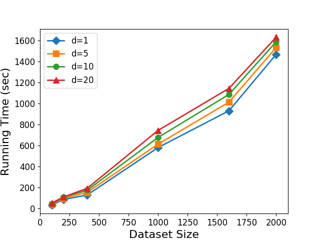
(a) Computation cost of ${\mathsf{PHC}}$.

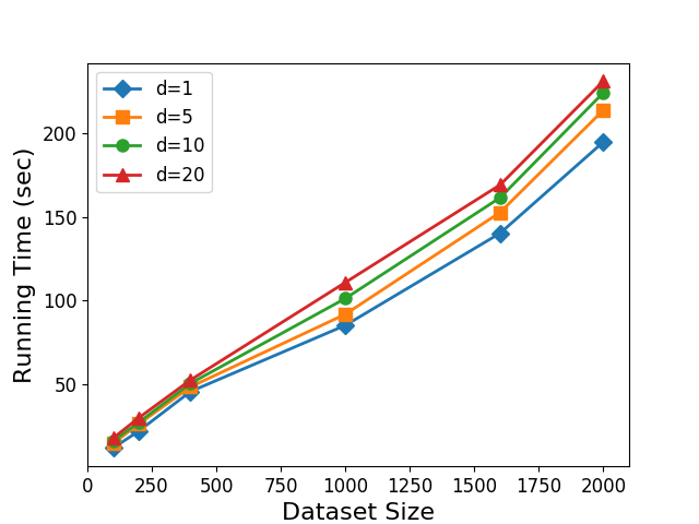
(b) Computation cost of ${\mathsf{OPT}}$.

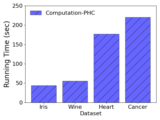
(c) Real-data performance of ${\mathsf{PHC}}$.

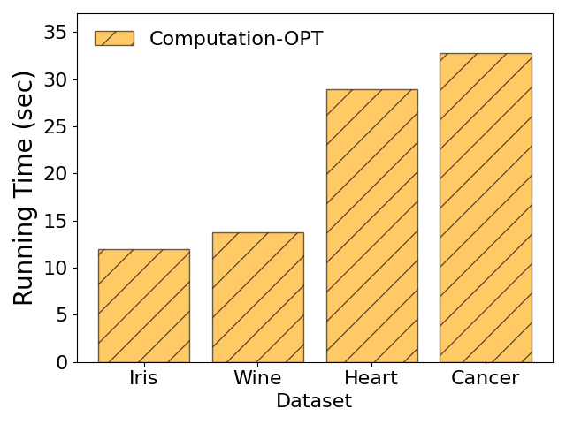
(d) Real-data performance of ${\mathsf{OPT}}$.

Figure 6. Performance of ${\mathsf{PHC}}$ (left) Vs. ${\mathsf{OPT}}$ (right).

We generate synthetic $d$-dimensional datasets of sizes up to 1M records and $d\in[1,20]$, using a Gaussian mixture distribution, as follows: (1) The number of clusters is randomly chosen in $[8:15]$; (2) Each cluster center is randomly chosen in $[-50,50]^{d}$ (performance is dominated by $\kappa$ but not exact data values), subject to a minimum-separation distance between pairs; (3) Cluster standard deviation is randomly chosen in $[0.5,4$]; and (4) Outliers are selected uniformly at random in the same interval and assigned randomly to clusters to emulate 3 noise percentage scenarios: low $0.1\%$, medium $1\%$, and high $5\%$. We randomly split each dataset into two halves which form the private inputs of the parties. We set the number of target clusters to $\ell_{t}=5$; as our protocol incurs costs linear in the number of iterations ($n-\ell_{t}$), this choice comprises a worst-case setting, as in practice more than 5 target clusters are desired.

We adapted our protocols to support floating point numbers. Here, due to the simplicity of the involved operations, we can rely on fixed-precision floating point numbers and it suffices to multiply floating point values by a constant $K$ (e.g. $K=2^{20}$ for IEEE 754 doubles). During ${\mathsf{PHC}}.{\mathsf{Setup}}$, we can achieve higher precision. After each party decrypts the blinded values (line 2 and line 2), they can re-scale by dividing the constant $K$ without affecting precision. During ${\mathsf{Cluster}}$, as we only merge the points based on the comparisons between the distances, multiplying by a constant does not affect the results.

Finally, we use the ABY C++ framework (Demmler et al., 2015), $128$-bit AES for GC, $1024$-bits Pailler, and set $\kappa=40$. We use libpaillier (lib, 2019) for Paillier encryption. We run our experiments on a 24-core machine, running Scientific Linux with 128GB memory on 2.9GHz Intel Xeon.

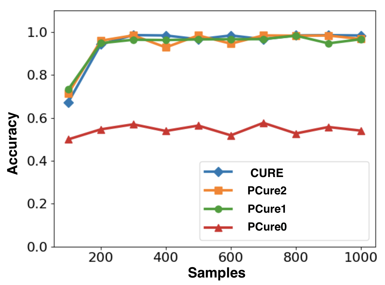
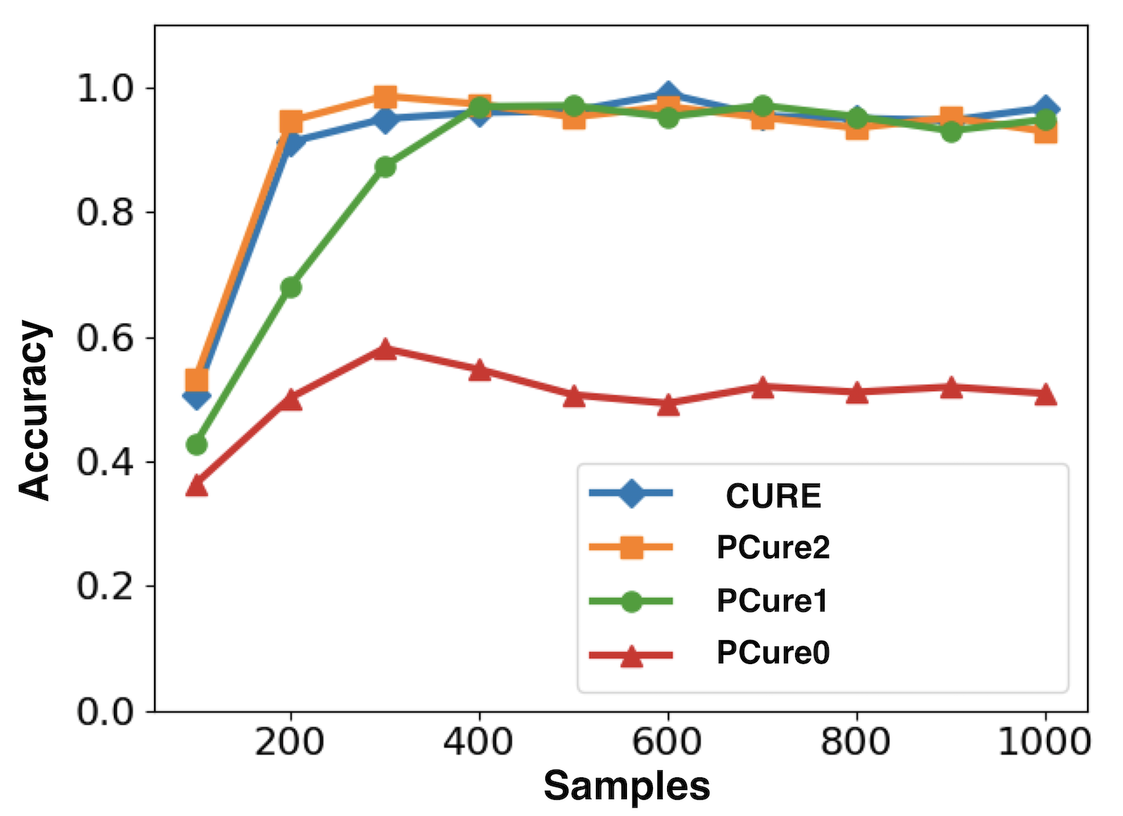
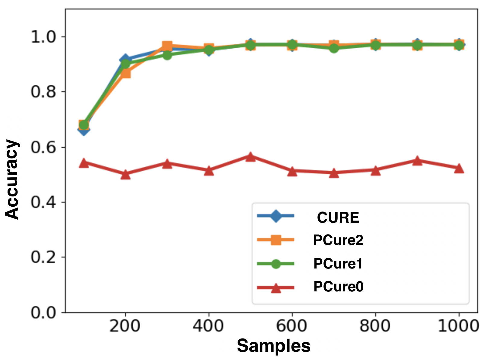
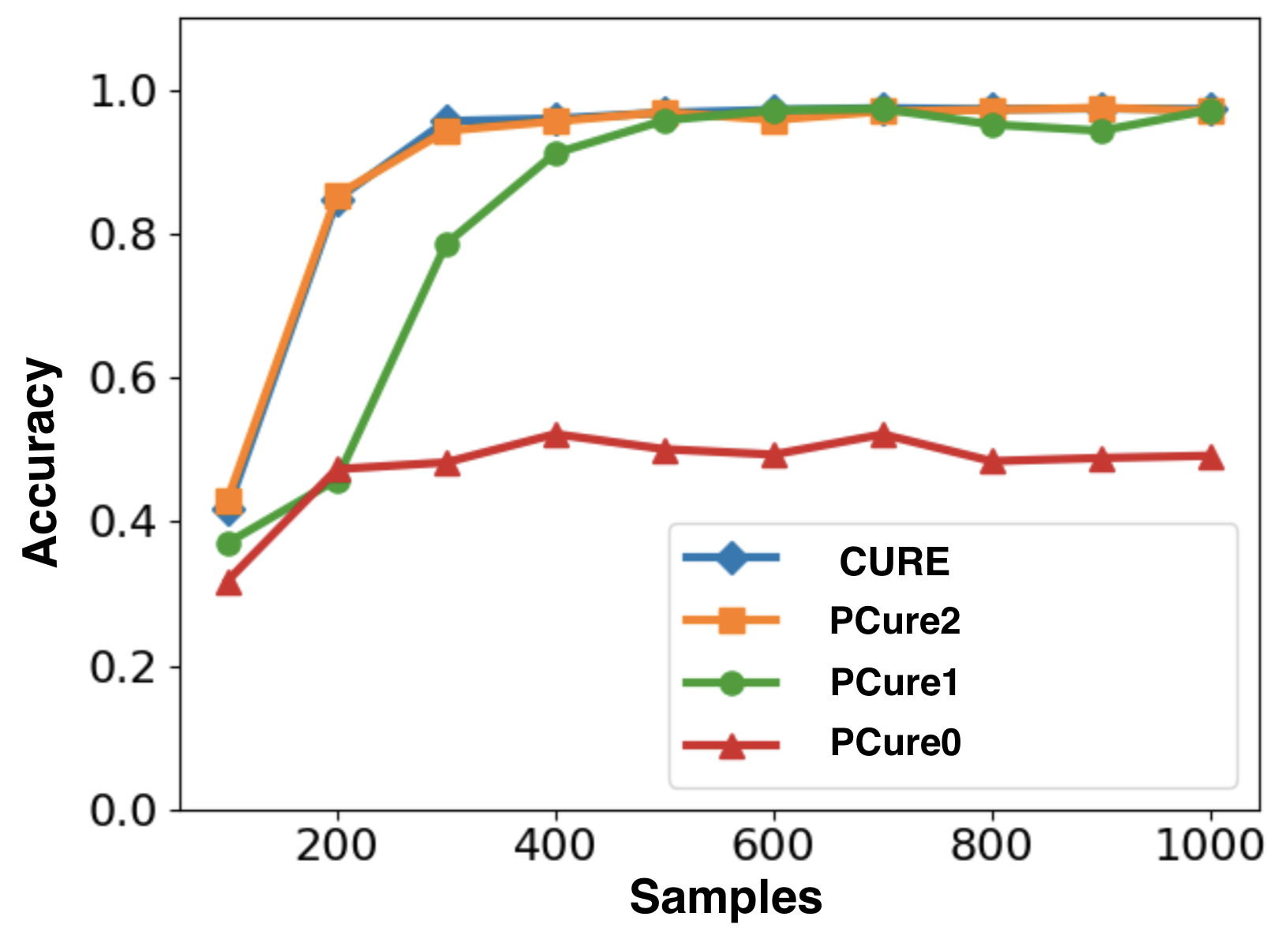
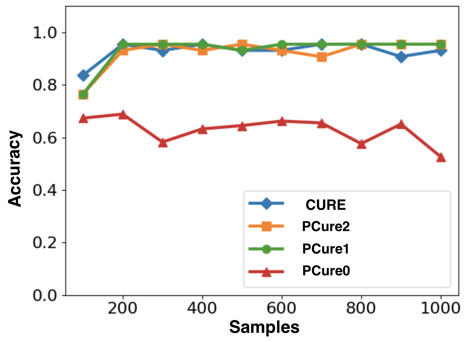
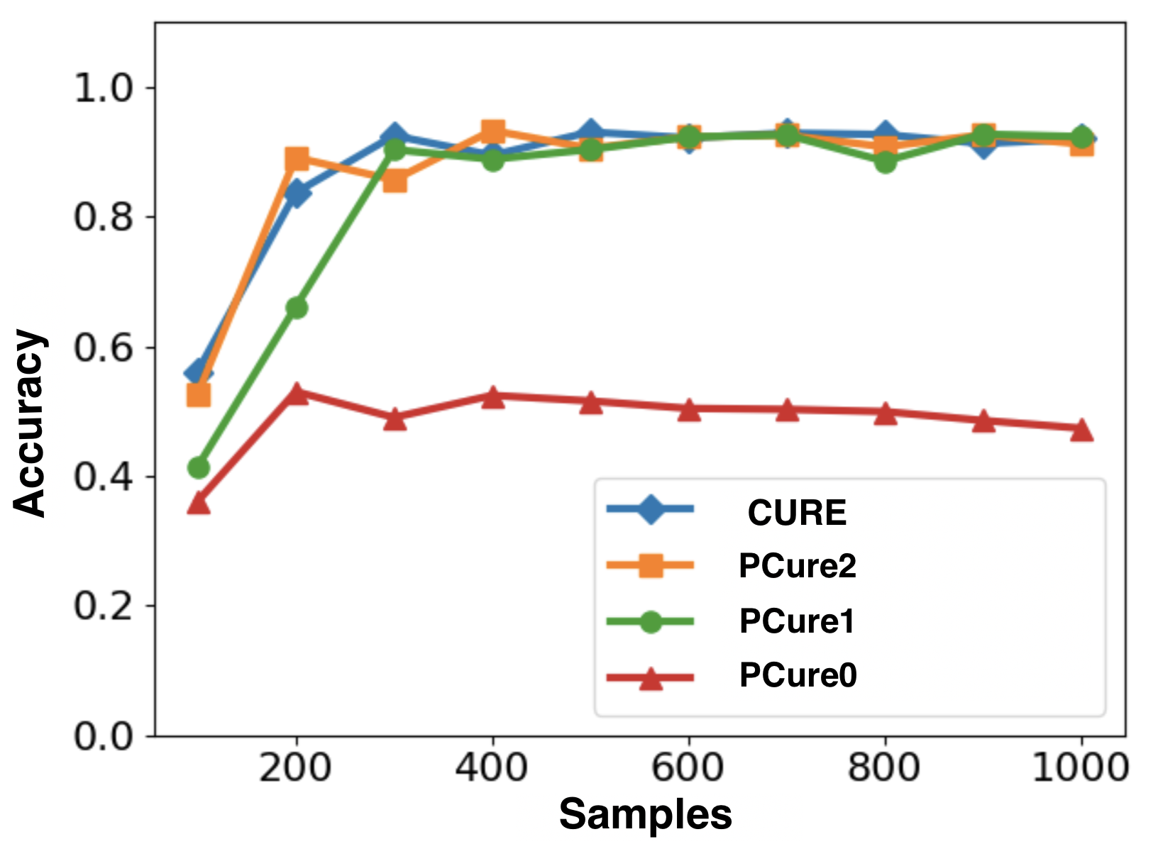
Figure 7. Accuracy of $\mathsf{CURE}$, $\mathsf{PCure*}$: $p=1$ (left), $p=5$ (right), #outliers = $0.1\%$ (top), $1\%$ (middle), $5\%$ (bottom).

Protocol ${\mathsf{PHC}}$. We first report results on the performance of our ${\mathsf{PHC}}$ protocol from Section 4. Figure 6(a) shows the computational cost for synthetic datasets of various sizes and dimensions, averaged over single and complete linkages. First, consistently with our analysis in Section 5, dimensions have minimal impact, since ${\mathsf{PHC}}$’s performance relates primarily to computing inter-cluster distances that is minimally affected by $d$. As expected its cubic asymptotic complexity, the overhead increases steeply with dataset size $n$.

Protocol ${\mathsf{OPT}}$. Figure 6(b) shows the computational costs on synthetic datasets for our optimized single-linkage variant ${\mathsf{OPT}}$ (with configurations identical to those for ${\mathsf{PHC}}$). In line with our analysis in Section 5, ${\mathsf{OPT}}$ significantly improves performance, reducing running time by an order of magnitude. E.g., for datasets of $2000$ $20$-dimensional points, the running time is approximately $230$ secs, an $8\times$ speedup compared to ${\mathsf{PHC}}$. The difference in our above example,is explained by the following observations: (1) although ${\mathsf{OPT}}$ improves performance during clustering by a linear factor, it adds costs during setup; and (2) the involved constants of the quadratic costs are higher for running time in setup phase, and vice versa in clustering phase. As shown in Figure 6(d), ${\mathsf{OPT}}$ significantly improves performance over ${\mathsf{PHC}}$, also when tested over our real datasets.

Protocols $\mathsf{PCure*}$. Figure 7 shows the accuracy of our $\mathsf{CURE}$-variant protocols $\mathsf{PCure0}$, $\mathsf{PCure1}$, $\mathsf{PCure2}$ from Section 6, and the non-private $\mathsf{CURE}$ algorithm on synthetic datasets of 1M records for $10^{2}$–$10^{3}$ samples, partition parameters $p=1$ and $p=5$, and for low (0.1%), medium (1%), and high (5%) outliers-to-data percentages. Clearly, $\mathsf{PCure0}$, where parties run $\mathsf{CURE}$ on their own samples, without any interaction besides announcing representatives for individually computed clusters, exhibits very poor accuracy. e.g., $44.4$% loss for 1M records. For $p=1$, $\mathsf{PCure1}$ and $\mathsf{PCure2}$ achieve similar accuracy, which approaches that of $\mathsf{CURE}$ for large enough samples: At 300 samples or higher, the gap is within 3%. For higher values of $p$, e.g., $p=5$, $\mathsf{PCure1}$ and $\mathsf{PCure2}$ exhibit a difference in accuracy: E.g., at 200 samples the accuracy for $\mathsf{PCure1}$ is lower by 39.54% than $\mathsf{PCure2}$; but at 500 samples or more, they are within 3.18%.

Moreover, experimenting with all combinations of $p=1,3,5$ partitions and $R=1,3,5,7,10$ representatives shows that the accuracies of $\mathsf{PCure2}$ and $\mathsf{PCure1}$ are very close to $\mathsf{CURE}$ at $s=1000$ samples (or more). The largest observed difference between $\mathsf{PCure1}$ and $\mathsf{CURE}$ is 3.57%, and between $\mathsf{PCure2}$ and $\mathsf{CURE}$ is 2.7%. For $p=1$ and $R=1$ either difference is less than 1% at 1000 samples (or more). Thus, our choice of $p=1$ and $R=1$ to protect data privacy, as argued in Section 6, does not impact the protocol’s accuracy.

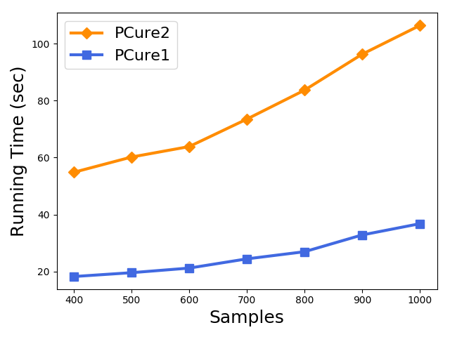
Figure 8. End-to-end computation of $\mathsf{PCure1}$, $\mathsf{PCure2}$.

We also compare end-to-end computation for $\mathsf{PCure1}$ and $\mathsf{PCure2}$ (with ${\mathsf{OPT}}$), $n=10^{6}$, $d=10$, $1\%$ outliers, no sample partitioning ($p=1$), $\ell_{t}=5$ target clusters, and $q=3$ for A-Clustering. Figure 8 shows their good performance for sample sizes $s\in[400:1000]$. For $10^{3}$ samples, $\mathsf{PCure2}$ runs in $104$sec, while $\mathsf{PCure1}$ runs in $35$sec – $3\times$ faster, but with similar accuracy 97.09%.

Network Latency Impact. Although our experiments show the efficiency of our schemes, if executed over WAN this would be affected by network latency and data transmission. To estimate this impact, we considered two AWS machines in us-east and us-west and measured their latency to $50-60$ms. Taking $\mathsf{PCure2}$ with $400$ samples and $\ell_{t}=5$ as our use case, a single clustering round with four roundtrips (assuming distance update is done with a single garbled circuit) would take approximately $200$-$240$ms. Regarding data transmission of the two garbled circuits for finding the minimum distance and updating the cluster distances, using the circuits for addition/subtraction, comparison, and min-index-selection from (Kolesnikov et al., 2009) for $100$, $64$-bit values, we estimate their size as roughly $10$MB (not including the OT data which is dominated by the circuits). Under the mild assumption of a $100$Mbps connection, transmission would take ${\sim}800$ms for a total of ${\sim}1$sec. In subsequent rounds, the circuits become progressively smaller but the number of roundtrips remains the same; even conservatively multiplying by $395$ rounds, we have approximately $400$sec of total communication time. For comparison, in Figure 8, for the same setting computation takes ${\sim}55$sec.

Hence, communication indeed becomes a bottleneck for our schemes when run over WAN, but not to the point where they are entirely impractical. Furthermore, our goal when implementing our schemes was not to minimize end-to-end latency but computation, so there is plenty of room for optimizations. E.g., our protocols can be run in “round batches” merging $k$ clusters with one interaction (by larger circuits) which would decrease RTTs by a factor of $k$. Finally, dedicated cloud technologies, such as AWS VPC (vpc, 2021), can offer private connections drastically reducing communication time.

8. Related Work

Secure machine learning. There exists a rapidly growing line of works that propose secure protocols for a variety of ML tasks. This includes constructions for private classification models in the supervised learning setting (such as decision trees (Lindhell and Pinkas, 2000), SVM classification (Vaidya et al., 2008), linear regression (Du and Atallah, 2001; Du et al., 2004; Sanil et al., 2004), logistic regression (Fienberg et al., 2006) and neural networks (Orlandi et al., 2007; Barni et al., 2011; Sadeghi and Schneider, 2008)), as well as federated learning tasks (Bonawitz et al., 2017). Another focus has been on proposing MPC-based protocols that are provably secure under a well-defined real/ideal definition, similar to ours (e.g., (Bost et al., 2015; Nikolaenko et al., 2013; Gascón et al., 2017; Gilad-Bachrach et al., [n.d.]; Aono et al., 2016; Chabanne et al., 2017; Riazi et al., [n.d.]; Rouhani et al., 2018; Liu et al., 2017; Chandran et al., [n.d.]; Hesamifard et al., [n.d.]; Gilad-Bachrach et al., 2016; Mohassel and Zhang, 2017; Li et al., 2018; Juvekar et al., [n.d.])), for numerous tasks with a focus on neural networks and deep learning.

The above works can be split into two categories: those that focus on private model training and those that focus on private inference/classification. In our unsupervised setting, our protocol protects the privacy of the parties’ data during the clustering phase.

Deployed techniques. In terms of techniques, most works use (some variant of) homomorphic encryption (e.g., (Paillier, 1999; Gentry, 2009)). More advanced ML tasks often require hybrid techniques, e.g., combining the above with garbled circuits (e.g., (Rouhani et al., 2018)) or other MPC techniques (Riazi et al., [n.d.]; Mishra et al., [n.d.]). Our construction adopts such “mixed” techniques for the problem of hierarchical clustering. More recently, solutions have been proposed based on trusted hardware (such as Intel SGX), e.g., (Ohrimenko et al., [n.d.]; Tramèr and Boneh, [n.d.]; Chamani and Papadopoulos, 2020). This avoids the need for “heavy” cryptography, however, it weakens the threat model as it requires trusting the hardware vendor. Finally, a different approach seeks privacy via data perturbation (Abadi et al., 2016; Chaudhuri and Monteleoni, 2008; Song et al., 2013; Chase et al., 2017; Oliveira and Zaïane, 2003; Shokri and Shmatikov, 2015), by adding statistical noise to hide data values, e.g., differential privacy (Dwork et al., 2006). Such techniques are orthogonal to the cryptographic methods that we apply here but they can potentially be combined (e.g., as in (Pettai and Laud, 2015)). Using noise to hide whether a specific point has been included in a given cluster would be complement very nicely our cluster-information-reduction approach, potentially leading to more robust security treatment.

Privacy-preserving clustering. Many previous works proposed private solutions for different clustering tasks with the majority focusing on the popular, but conceptually simpler, $k$-means problem (e.g., (Vaidya and Clifton, 2003; Jagannathan and Wright, 2005; Jha et al., 2005; Bunn and Ostrovsky, 2007; Doganay et al., 2008; Erkin et al., 2013; Mohassel et al., 2020; Rao et al., 2015; Jäschke and Armknecht, 2018; Kim and Chang, 2018)) and other partitioning-based clustering methods (e.g., (Keller et al., 2021; Zhang et al., 2017)). Fewer other works consider private density-based (Cheon et al., 2019; Zahur and Evans, 2013; Bozdemir et al., 2021) or distribution-based (Hamidi et al., 2018) clustering. An in-depth literature survey and comparative analysis of private clustering schemes can be found in the recent work of (Hegde et al., 2021).

Focusing on private hierarchical clustering, no previous work offers a formal security definition, relying instead on ad-hoc analysis (Inan et al., 2007; Jagannathan et al., 2010; Sheikhalishahi and Martinelli, 2017; De and Tripathy, 2014; Jagannathan et al., 2006). Moreover some schemes leak information to the participants that can clearly be harfmul—and is much more than what our protocol reveals—e.g., (Sheikhalishahi et al., [n.d.]; Tripathy and De, 2013) reveal all distances across parties’ records. One notable exception is the scheme of Su et al. (Su et al., 2014) which, however, is designed specifically for the case of document clustering. Here, we proposed a security formulation within the widely studied read/ideal paradigm of MPC that characterizes precisely what information is revealed to the collaborating parties. Besides making it easier to compare our solution with potential future ones that follow our formulation, this is, to the best of our knowledge the only private hierarchical clustering scheme with formal proofs of security. Finally, it is an interesting problem to combine optimizations for “plaintext” clustering (e.g.,(Murtagh and Contreras, 2017; Olson, 1995; Cohen-Addad et al., [n.d.])) with privacy-preserving techniques to improve efficiency.

Secure approximate computation. The interplay between cryptography and efficient approximation (Feigenbaum et al., 2006) has already been studied for pattern matching in genomic data (Wang et al., 2015; Asharov et al., 2018), $k$-means (Su et al., 2007), and logistic regression (Xie et al., 2016; Takada et al., 2016). To the best of our knowledge, ours is the first work to compose secure cryptographic protocols with efficient approximation algorithms for hierarchical clustering.

Leakage in machine learning. The significant impact of information leakage in collaborative, distributed, or federated learning has been the topic of a long line of research (e.g., see (Shokri and Shmatikov, 2015; Liu et al., 2021; Li et al., 2020; Al-Rubaie and Chang, 2019)). Various practical attacks have been demonstrated that infer information about the training data or the ML model and its hyper-parameters, (e.g., (Fredrikson et al., 2015; Hitaj et al., 2017; Shokri et al., 2017)). This is even more important in collaborative learning where parties could otherwise benefit from sharing data but such leakage may stop them (e.g., (Melis et al., [n.d.]; Zhao et al., 2020a, b; Yan et al., 2021)). Hence, it is crucial for our protocol to formally characterize what is the shared information for the two parties.

9. Conclusion

We propose the first formal security definition for private hierarchical clustering and design a protocol for single and complete linkage, as well as an optimized version. We also combine this with approximate clustering to increase scalability. We hope this work motivates further research in privacy-preserving unsupervised learning, including secure protocols for other linkage types (e.g., Ward), alternative approximation frameworks (e.g., BIRCH (Zhang et al., 1996)), different tasks (e.g., mixture models, association rules or graph learning), or schemes for more than two parties to benefit from larger-scale collaborations. Specific to our definition of privacy, we believe it would be helpful to experimentally and empirically evaluate the impact (even our significantly redacted) dendrogram leakage can have, e.g., by demonstrating possible leakage-abuse attacks.

Appendix A Garbled circuits

Garbled circuits (GC) (Yao, 1982, 1986) provide a general framework for securely realizing two-party computation of any functionality. The framework has been thoroughly studied in the literature (e.g., see formal treatments of the topic (Lindell and Pinkas, 2009; Bellare et al., 2012)) and we here overview the specific procedures involved in it.

In our running example, parties ${\mathsf{P_{1}}}$ and ${\mathsf{P_{2}}}$ wish to evaluate a specific function $f$ over their respective inputs $x_{1},x_{2}$ and engage in an interactive 2-phase protocol, where one party plays the role of the garbler and the other the role of the evaluator. Without loss of generality, ${\mathsf{P_{1}}}$ is the garbler and ${\mathsf{P_{2}}}$ is the evaluator, and their interaction proceeds as follows.

In phase I, ${\mathsf{P_{1}}}$ expresses $f$ as a Boolean circuit $\mathcal{C}_{f}$, i.e., as a directed acyclic graph of Boolean AND and OR gates, and then sends a “garbled,” i.e., encrypted, version of $\mathcal{C}_{f}$ to ${\mathsf{P_{2}}}$.

In our example, $\mathcal{C}_{f}$ corresponds to a circuit of two AND gates $A,B$ and an OR gate $C$, shown in Figure 9: Inputs $x_{1}$, $x_{2}$ are $11$ and $01$, and output $f(x_{1},x_{2})$ is 1, computed by feeding to the OR gate the two bitwise ANDs of the inputs.

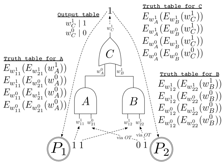
Figure 9. Garbled circuit $\mathcal{C}_{f}$ of a specific function $f$ that computes the OR over the pairwise ANDs of the 2-bit inputs.

To garble $\mathcal{C}_{f}$, ${\mathsf{P_{1}}}$ first maps (the two possible bits 0, 1 of) each wire $X$ in $\mathcal{C}_{f}$ to two random values $w^{0}_{X},w^{1}_{X}$ (from a large domain, e.g., $\{0,1\}^{128}$), called the garbled values of $X$.

Specifically, ${\mathsf{P_{1}}}$ maps the output wires of gates $A$, $B$, and $C$ to random garbled values $\{w_{A}^{0},w_{A}^{1}\},\{w_{B}^{0},w_{B}^{1}\}$ and respectively $\{w_{C}^{0},w_{C}^{1}\}$, and also maps the two input wires of gate $A$ (respectively, gate $B$) to random garbled values $\{w_{11}^{0},w_{11}^{1}\},\{w_{21}^{0},w_{21}^{1}\}$ (respectively, $\{w_{12}^{0},w_{12}^{1}\},\{w_{22}^{0},w_{22}^{1}\}$), where mnemonically the $i$-th input bit of party $\mathsf{P}_{j}$ corresponds to the $ij$-wire, $i,j\in\{1,2\}$.

Next, ${\mathsf{P_{1}}}$ sends to ${\mathsf{P_{2}}}$ the garbled truth table of every Boolean gate in $\mathcal{C}_{f}$, which is the permuted encrypted truth table of the gate, where row in the truth table is appropriately encrypted using the garbled values of its three associated wires. We only specify the garbled truth table of the AND gate $A$, as other gates can be handled similarly. The row $(1,1)\rightarrow 1$ in the truth table of $A$ dictates that the output is $1$ when input is $1,1$ or, using garbled values, that the output is $w_{A}^{1}$ when input is $w_{11}^{1},w_{21}^{1}$. Accordingly, using a semantically-secure symmetric encryption scheme $E_{k}(\cdot)$ (e.g., 128-bit AES), ${\mathsf{P_{1}}}$ can express this condition as ciphertext $E_{w_{11}^{1}}(E_{w_{21}^{1}}(w_{A}^{1}))$, where the output $w_{A}^{1}$ is successively encrypted using the inputs $w_{11}^{1},w_{21}^{1}$ as encryption keys. ${\mathsf{P_{1}}}$ produces a similar ciphetext for each other row in the truth table of $A$ and sends them to ${\mathsf{P_{2}}}$, permuted to hide the order of the rows. Observe that one can retrieve $w_{A}^{1}$ if and only if they possess both $w_{11}^{1},w_{21}^{1}$, and that if one possesses only $w_{11}^{1},w_{21}^{1}$, all other entries of the garbled truth table of $A$ (besides $w_{A}^{1}$) are indistinguishable from random, due to the semantic security of the encryption scheme $E_{k}(\cdot)$.

Finally, to allow ${\mathsf{P_{2}}}$ to retrieve the final output $f(x_{1},x_{2})$, ${\mathsf{P_{1}}}$ also sends the garbled values $w_{C}^{0},w_{C}^{1}$ of the output wire together with their corresponding mapping to 0 and 1. Note that ${\mathsf{P_{2}}}$ is no privy to any other mappings between wires’ garbled values and their possible bit values.

In phase II, ${\mathsf{P_{2}}}$ evaluates the entire circuit $\mathcal{C}_{f}$ over the received garbled truth tables of the gates in it, by evaluating gates one by one in the ordering hierarchy induced by (the DAG structure of) $\mathcal{C}_{f}$. Indeed, if ${\mathsf{P_{2}}}$ knows the $w$ value of each input wire of a gate and its garbled truth table, ${\mathsf{P_{2}}}$ can easily discover its output value, by attempting to decrypt all rows in the table and accepting only the one that returns a correct output value. For example, if ${\mathsf{P_{2}}}$ has $w_{11}^{1},w_{21}^{0}$, ${\mathsf{P_{2}}}$ can try to decrypt every value in the garbled truth table of $A$, until ${\mathsf{P_{2}}}$ finds the correct value $w_{A}^{1}$.

To initiate this circuit-evaluation process, ${\mathsf{P_{2}}}$ needs to learn the garbled values of each of the input wires in $\mathcal{C}_{f}$, which is achieved as follows: (1) ${\mathsf{P_{1}}}$ sends to ${\mathsf{P_{2}}}$ the $w$ values $w_{11}^{1},w_{12}^{1}$ corresponding to the input wires of ${\mathsf{P_{1}}}$ in the clear (note that since these are random values, ${\mathsf{P_{2}}}$ cannot map them to 0 or 1, thus ${\mathsf{P_{1}}}$’s input is protected); (2) ${\mathsf{P_{2}}}$ privately query from ${\mathsf{P_{1}}}$ the $w$ values $w_{21}^{0},w_{22}^{1}$ corresponding to the input wires of ${\mathsf{P_{2}}}$, that is, without ${\mathsf{P_{1}}}$ learning which garbled values were queried, via a two-party secure computation protocol called 1-out-of-2 oblivious transfer (OT) (Rabin, 1981). At a very high level, and focusing on a single input bit, OT allows ${\mathsf{P_{2}}}$ to retrieve from ${\mathsf{P_{1}}}$ exactly one value in pair ($w_{21}^{0}$, $w_{21}^{1}$) without ${\mathsf{P_{1}}}$ learning which value was retrieved. After running the OT protocol for every input bit, ${\mathsf{P_{2}}}$ can evaluate $\mathcal{C}_{f}$, as above, to finally compute and send back to ${\mathsf{P_{1}}}$ the correct output $f(x_{1},x_{2})=1$, deduced by the final garbled value $w_{C}^{1}$ of the output wire.

Appendix B Secure ${\mathsf{min}}$-selection protocols

Here, we overview the design of GC-based protocols ${\mathsf{ArgMin}}$ and ${\mathsf{MaxDist}}$/${\mathsf{MinDist}}$ for secure selection of min/max values, or their index/location, over secret-shared data. These protocols have been defined in Sections 4 and 5 and comprise integral components of our solutions. We provide the exact two circuits over which we can directly apply the garbled-circuits framework (see Appendix A) to get GC-protocols ${\mathsf{ArgMin}}$ and ${\mathsf{MinDist}}$, noting that the circuit in support of ${\mathsf{MaxDist}}$ is similar to the case of ${\mathsf{MinDist}}$.

Recall that data consists of $\lambda$-bit values and is secret shared among the two parties as $\kappa$-bit random blinding terms, $\kappa>\lambda$, and $\kappa+1$-bit blinded values, each resulted by adding a random blinding term to an ordinary data value.

Our circuits use as building blocks the following gates, efficient implementations of which are well studied (Kolesnikov et al., 2009):

• ADD/SUB that adds/subtracts $\kappa+1$-bit integers;

• MIN/MAX that selects the ${\mathsf{min}}/{\mathsf{max}}$ of two $\lambda$-bit integers, using a one-bit output to encode which input value is the ${\mathsf{min}}/{\mathsf{max}}$ value (e.g., on input $3,5$ MIN outputs 0 to indicate the first value is smaller);

• a multiplexer gate MUX_i that on input two $i$-bit inputs and a selector bit $s$, outputs the first or the second one, depending on the value of $s$; and finally

• hard-coded in the circuit constant gates CON_i, $1\leq i\leq n$, that always output the $(\log n)$-bit fixed value $i$ (e.g., CON₃ outputs the binary representation of $3$).

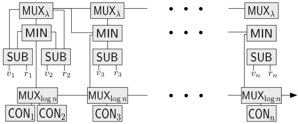
Figure 10. The circuit for protocol $\mathsf{{\mathsf{ArgMin}}}$.

Figure 10 shows the circuit of protocol $\mathsf{{\mathsf{ArgMin}}}$ for selecting the index of the minimum value in an array of $n$ different values. On input $n$ $\kappa+1$-bit values $v_{1},\dots,v_{n}$ and $n$ $\kappa$-bit blinding terms $r_{1},\dots,r_{n}$, the circuit first uses $n$ SUB gates to compute (the secret) values $v_{i}-r_{i}$, $i=1,\dots,n$, and then selects the index of the minimum such value in $n-1$ successive comparisons as follows. In the $i$th comparison, a MIN gate compares the currently minimum value $m_{i}$ of index $loc_{i}$ (initially, $m_{1}=v_{1}-r_{1}$, $loc_{1}=1$) to value $v_{i+1}-r_{i+1}$ of index $i+1$, and its output bit is fed, as the selector bit, to two multiplexer gates MUX_μ:

• $\mu=\log n$: once for selecting among two $(\log n)$-bit indices $loc_{i}$ and $i+1$, the latter conveniently encoded as the output of constant gate CON_i+1 (such hard-coded indices significantly facilitate their propagation in the circuit, compared to the alternative of handling indexes as input and carrying them over throughout the circuit); and

• $\mu=\lambda$: once for selecting among two $\lambda$-bit values $m_{i}$ and $v_{i+1}-r_{i+1}$,

overall propagating the updated minimum value $m_{i+1}={\mathsf{min}}\{a,b\}$ and its index $loc_{i+1}$ to the next $(i+1)$th comparison. The final output (see arrow wire) corresponds to the output of the $(n-1)$th index-selection multiplexer gate.

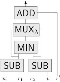
Figure 11. The circuit for protocol ${\mathsf{MinDist}}$.

Figure 11 shows the circuit for protocol ${\mathsf{MinDist}}$ for selecting and re-blinding the minimum value among two secret-shared values. On input two $\kappa+1$-bit blinded values $u,v$ and three $\kappa$-bit blinding terms $r_{1},r_{2},r^{\prime}$, the circuit first computes $u-r_{1}$, $v-r_{2}$ using two SUB gates, then computes the minimum of these two values using a MIN gate, and its output bit is fed, as the selector bit, to a multiplexer gate MUX_λ for selecting the minimum among two $\lambda$-bit values $u-r_{1}$ and $v-r_{2}$, which is becomes the final output (see arrow wire) after it is blinded by adding the input blinding term $r^{\prime}$ through a ADD gate. (The circuit for protocol ${\mathsf{MaxDist}}$ is the same with a MAX gate replacing the MIN gate.)

Appendix C Proof of Theorem 5.1

We begin by recalling that, under the assumption that the oblivious transfer protocol used is secure, there exists simulator $\mathsf{Sim}_{OT}$ that can simulate the views of each of the parties ${\mathsf{P_{1}}},{\mathsf{P_{2}}}$ during a single oblivious transfer execution when given as input the corresponding party’s input (and output, in case it is non-empty) and randomness.

The core idea behind our proof is that, since all values seen by the two parties during the protocol execution (apart from the indexes of the merged clusters at each clustering round) are “blinded” by large random factors, these values can be perfectly simulated, as needed in our proof, by randomly selected values. For example, assuming all values $p_{i},q_{i}$ are 32-bits and the chosen random values are 100-bits, it follows that the sum of the two is statistically indistinguishable from a 100-bit value chosen uniformly at random. In particular, this allows the simulator to effectively run the protocol with the adversary by simply choosing simulated values for the other party which he chooses himsellf at random (in the above example these would be random 32-bit values).

We handle the two cases of party corruption separately.

Corruption of ${\mathsf{P_{2}}}$. The view of ${\mathsf{P_{2}}}$ during the protocol execution consists of:

1. Encrypted matrices $B,R$ and encrypted arrays $L,S$.

2. For each clustering round $\ell$, messages received during the oblivious transfer execution for $\mathsf{ArgMin}$, denoted by $OT_{\ell}$ and the min/max index $\alpha_{\ell}$.

3. During each clustering round $\ell$, for each execution of ${\mathsf{MinDist}}$/${\mathsf{MaxDist}}$ for index $k$, messages received during the corresponding oblivious transfer execution, denoted by $OT_{\ell,k}$, corresponding garbled circuit $GC_{\ell,k}$, and output value $v_{\ell,k}$.

4. Encrypted cluster representative values $E_{1},\dots,E_{\ell_{t}}$.

The simulator $\mathsf{Sim}_{P_{2}}$, on input the random tape $R_{2}$, points $q_{1},\dots,q_{n_{2}}$, outputs $(rep_{1}/|J_{1}|,|J_{1}|,\dots,rep_{\ell_{t}}/|J_{\ell_{t}}|,|J_{\ell_{t}}|)$, $\alpha_{1},\dots,\alpha_{\ell_{t}}$, computes the view of ${\mathsf{P_{2}}}$ as follows.

• (Ciphertext computation) Using random tape $R_{2}$, the simulator runs the key generation algorithm for ${\mathsf{P_{2}}}$ to receive $sk^{\prime},pk^{\prime}$. He then chooses values $p^{\prime}_{1},\dots,p^{\prime}_{n_{1}}$ uniformly at random from $\{0,1\}^{d}$. These will act as the “simulated” values for player ${\mathsf{P_{1}}}$. He then runs protocol ${\mathsf{PHC}}$ honestly using the values $p^{\prime}_{i}$ as input for ${\mathsf{P_{1}}}$ (and the actual values $q_{i}$ of ${\mathsf{P_{2}}}$), with the following modifications.

• (Oblivious transfer simulation for $OT_{\ell}$) For $\ell=1,\dots,\ell_{t}$ let $W_{\ell}$ be the set of garbled input values computed by ${\mathsf{P_{2}}}$ for the garbled circuit that evaluates ${\mathsf{MinDist}}$/${\mathsf{MaxDist}}$ at clustering round $\ell$. Since we are in the semi-honest setting, the corrupted ${\mathsf{P_{2}}}$ computes these values uniformly at random. Therefore, the simulator can also compute them using $R_{2}$. Then, for $i=1,\dots,\ell,$ the simulator includes in the view (instead of $OT_{\ell}$) the output $OT^{\prime}_{\ell}$ produced by simulator $\mathsf{Sim}_{OT}^{(2)}$ on input $W_{\ell}$. Note that ${\mathsf{P_{2}}}$ does not receive any output from this oblivious transfer execution, thus $\mathsf{Sim}_{OT}^{(2)}$ only works given the input.

• (Oblivious transfer simulation for $\mathsf{Argmin}$) For each clustering round $\ell$, the simulator includes in the view, the index $\alpha_{\ell}$.

• (Garbled circuit simulation for $GC_{\ell,k}$) Next, the simulator needs to compute the garbled circuits $GC_{\ell,k}$. The simulator uses the corresponding values from $\mathcal{R}$ (as computed so far) and a “new” blinding factor $\rho_{\ell,k}$ for ${\mathsf{P_{1}}}$’ inputs and computes a garbled circuit for evaluating $\mathsf{ArgMin}$ honestly. The simulator also includes in the view of ${\mathsf{P_{2}}}$ the garbled inputs for the corresponding elements from $\mathcal{R}$.

• (Oblivious transfer simulation for $OT_{\ell,k}$) Let $y_{\ell,k}$ be the input of ${\mathsf{P_{2}}}$ for the circuit $GC_{\ell,k}$ (i.e., the execution of ${\mathsf{ArgMin}}$ for index $k$ during clustering round $\ell$). Since we are in the semi-honest case, the corrupted ${\mathsf{P_{2}}}$ will provide as input the values that have been established from the interaction with ${\mathsf{P_{1}}}$ (using the points $p^{\prime}_{i}$) up to that point, therefore $y_{\ell,k}$ can be computed by the simulator. In order to compute the parts of the view that correspond to each of $OT_{\ell,k}$ the simulator includes in the view the output of $\mathsf{Sim}_{OT}$ on input $y_{\ell,k}$ and the corresponding choice from each pair of garbled inputs he chose in the previous step (as dictated by the bit representation of $y_{\ell,k}$), which we denote as $OT^{\prime}_{\ell,k}$.

• (Encrypted representatives computation) For $\ell=1,\dots,\ell_{t}$, the simulator computes $rep_{\ell}=\lceil rep_{\ell}/|J_{\ell}|\cdot|J_{i}|\rceil$ and $E_{\ell}=[rep_{\ell}]$, where encryption is under (the previously computed) $pk$.

We now argue that the view produced by our simulator is indistinguishable from the view of ${\mathsf{P_{2}}}$ when interacting with ${\mathsf{P_{1}}}$ running ${\mathsf{PHC}}$. This is done via the following sequence of hybrids.

Hybrid 0. This is the view $\mathsf{view}_{\mathcal{A}^{{\mathsf{PHC}}}_{P_{2}}}$, i.e., the view of ${\mathsf{P_{2}}}$ when interacting with ${\mathsf{P_{1}}}$ running ${\mathsf{PHC}}$ for points $p_{i}$.

Hybrid 1. This is the same as Hybrid 0, but the output of $GC_{\ell}$ in $\mathsf{view}_{\mathcal{A}^{{\mathsf{PHC}}}_{P_{2}}}$ is replaced by $\alpha_{\ell}$. This is indistinguishable from Hybrid 0 due to the correctness of the garbling scheme. Since we are in the semi-honest setting, both parties follow the protocol, therefore the outputs they evaluate are always $\alpha_{\ell}$.

Hybrid 2. This is the same as Hybrid 1, but values in $B,L$ are computed using values $p^{\prime}_{i}$. This is statistically indistinguishable from Hybrid 1 (i.e., even unbounded algorithms can only distinguish between the two with probability $O(2^{\kappa}$) since in $\mathsf{view}_{\mathcal{A}^{{\mathsf{PHC}}}_{P_{2}}}$, each of the values in $B,L$ are computed as the sum of a random value from $\{0,1\}^{\kappa}$ and a distance between two clusters.

Hybrid 3. This is the same as Hybrid 2, but all values in $R,S$ are replaced with encryptions of zero’s. This is indistinguishable from Hybrid 2 due to the semantic security of Paillier’s encryption scheme.

Hybrid 4. This is the same as Hybrid 3, but each of $OT_{\ell}$ is replaced by $OT^{\prime}_{\ell}$, computed as described above. This is indistinguishable from Hybrid 3 due to the security of the oblivious transfer protocol.

Hybrid 5. This is the same as Hybrid 4, but the garbled inputs given to ${\mathsf{P_{2}}}$ for $GC_{\ell,k}$ are chosen based on the values that have been computed using values $p^{\prime}_{i}$. Since garbled inputs are chosen uniformly at random (irrespectively of the actual input values), this follows the same distribution as Hybrid 3.

Hybrid 6. This is the same as Hybrid 5, but each of $OT_{\ell,k}$ is replaced by output of $OT_{\ell,k}$ computed as described above. This is indistinguishable from Hybrid 5 due to the security of the oblivious transfer protocol.

Hybrid 7. This is the same as Hybrid 6, but each value $E_{i}$ sens to ${\mathsf{P_{2}}}$ is computed as $[\lceil rep_{i}/|J_{i}|\cdot|J_{i}|\rceil]$ using public key $pk^{\prime}$. This is indistinguishable from Hybrid 6 since we are in the semi-honest setting and both parties follow the protocol therefore the outputs they evaluate are always $rep_{i}/|J_{i}|$.

Note that Hybrid 7 corresponds to the view produced by our simulator and Hybrid 0 to the view that ${\mathsf{P_{2}}}$ receives while interacting with ${\mathsf{P_{1}}}$ during $\pi_{HC}$ which concludes this part of the proof.

Corruption of ${\mathsf{P_{1}}}$. The case where ${\mathsf{P_{1}}}$ is corrupted is somewhat simpler as he does not receive any outputs from the circuits $GC_{\ell,k}$. The view of ${\mathsf{P_{1}}}$ during the protocol execution consists of:

1. Encrypted tables $D,R$ and encrypted arrays $H,L,S$.

2. For each clustering round $\ell$, a garbled circuit $GC_{\ell}$ for evaluating $\mathsf{ArgMin}$, messages received during the corresponding oblivious transfer execution denoted by $OT_{\ell}$.

3. During each clustering round $\ell$, for each execution of ${\mathsf{MinDist}}$/${\mathsf{MaxDist}}$ for index $k$, messages received during the corresponding oblivious transfer execution denoted by $OT_{\ell,k}$.

The simulator $\mathsf{Sim}_{P_{1}}$, on input the random tape $R_{1}$, points $p_{1},\dots,p_{n_{1}}$, outputs $(rep_{1}/|J_{1}|,|J_{1}|,\dots,rep_{\ell_{t}}/|J_{\ell_{t}}|,|J_{\ell_{t}}|)$, $\alpha_{1},\dots,\alpha_{\ell_{t}}$, computes the view of ${\mathsf{P_{1}}}$ as follows.

• (Ciphertext computation) Using random tape $R_{1}$, the simulator runs the key generation algorithm for ${\mathsf{P_{1}}}$ to receive $sk,pk$ and computes a pair $sk^{\prime},pk^{\prime}$ for himself. He computes $D,H,L$ consisting of encryptions of zeros under $pk^{\prime}$. Moreover, he computes $R$,$S$ consisting of encryption of values chosen uniformly at random from $\{0,1\}^{\kappa}$ and encrypted under $pk$.

• (Garbled circuit simulation for $GC_{\ell}$) Next the simulator needs to provide garbled circuits for the evaluation of $\mathsf{ArgMin}$ for each clustering round $\ell$. For this, the simulator creates a “rigged” garbled circuit $GC^{\prime}_{\ell}$ that always outputs $\alpha_{\ell}$, irrespectively of the inputs. This is achieved by forcing all intermediate gates to always return the same garbled output and by setting the output translation temple to always to decode to the bit-representation of $\alpha_{\ell}$ (this process is explained formally in (Lindell and Pinkas, 2009)).

• (Oblivious transfer simulation for $\mathsf{ArgMin}$) Let $W^{(1)}_{\ell}$, $W^{(2)}_{\ell}$ be the sets of pairs of input garbled values that the simulator choses while creating $GC^{\prime}_{\ell}$ as described above (where the former corresponds to the input of ${\mathsf{P_{1}}}$ and the latter to the input of ${\mathsf{P_{2}}}$). The simulator includes in the view a random choice from each pair in $W^{(2)}$. Moreover, he replaces the messages in the view that correspond to the execution of $OT_{\ell,k}$, by the output of $\mathsf{Sim}_{OT}^{(1)}$ on input $(y_{\ell},W^{(1)}_{\ell})$, where $y_{\ell}$ is the bit description of the input of ${\mathsf{P_{1}}}$ for $GC_{\ell}$ (which can be computed with the simulator since he has access to $p_{i}$, $R_{1}$).

• (Oblivious transfer simulation for ${\mathsf{MinDist}}$/${\mathsf{MaxDist}}$) For each $GC_{\ell,k}$ let $W_{\ell,k}$ be the set of garbled input values computed by ${\mathsf{P_{1}}}$ for the garbled circuit that evaluates ${\mathsf{MinDist}}$/${\mathsf{MaxDist}}$ at clustering round $\ell$ and cluster $k$. Since we are in the semi-honest setting, the corrupted ${\mathsf{P_{1}}}$ computes these values uniformly at random. Therefore, the simulator can also compute them using random tape $R_{1}$. Then, for each $\ell,k$ the simulator includes in the view (instead of $OT_{\ell,k}$) the output $OT^{\prime}_{\ell,k}$ produced by simulator $\mathsf{Sim}_{OT}^{(1)}$ on input $W_{\ell,k}$ (and corresponding randomness derived from $R_{1}$). Note that ${\mathsf{P_{1}}}$ does not receive any output from this oblivious transfer execution, thus $\mathsf{Sim}_{OT}^{(1)}$ only works given the input.

We now argue that the view produced by our simulator is indistinguishable from the view of ${\mathsf{P_{1}}}$ when interacting with ${\mathsf{P_{2}}}$ running ${\mathsf{PHC}}$. This is done via the following sequence of hybrids.

Hybrid 0. This is the view $\mathsf{view}_{\mathcal{A}^{{\mathsf{PHC}}}_{P_{1}}}$, i.e., the view of ${\mathsf{P_{1}}}$ when interacting with ${\mathsf{P_{2}}}$ running $\pi_{HC}$ for points $q_{i}$.

Hybrid 1. This is the same as Hybrid 0, but all values in $D,H^{\prime},L$ are replaced with encryptions of zero’s. This is indistinguishable from Hybrid 1 due to the semantic security of Paillier’s encryption scheme.

Hybrid 2. This is the same as Hybrid 1, but values in $R,S$ are computed as encryptions of values chosen uniformly at random from $\{0,1\}^{\kappa}$ under key $pk$. This is statistically indistinguishable from Hybrid 1 for the same reasons as for the case of ${\mathsf{P_{2}}}$ above.

Hybrid 3. This is the same as Hybrid 2, but each of $GC_{\ell}$ is replaced by $GC^{\prime}_{\ell}$, computed as described above (including the values from $W_{(2)})$ This is indistinguishable from Hybrid 2 due to the security of encryption scheme used for the garbling scheme (this is formally described in (Lindell and Pinkas, 2009)).

Hybrid 4. This is the same as Hybrid 3, but each of $OT_{\ell}$ is replaced by $OT^{\prime}_{\ell}$, computed as described above. This is indistinguishable from Hybrid 3 due to the security of the oblivious transfer protocol.

Hybrid 5. This is the same as Hybrid 4, but each of $OT_{\ell,k}$ is replaced by $OT^{\prime}_{\ell,k}$ computed as described above. This is again indistinguishable from Hybrid 5 due to the security of the oblivious transfer protocol.

Note that Hybrid 5 corresponds to the view produced by our simulator and Hybrid 0 to the view that ${\mathsf{P_{2}}}$ receives while interacting with ${\mathsf{P_{1}}}$ during ${\mathsf{PHC}}$ which concludes this part of the proof.