Explaining Wrong Queries Using Small Examples

Abstract.

For testing the correctness of SQL queries, e.g., evaluating student submissions in a database course, a standard practice is to execute the query in question on some test database instance and compare its result with that of the correct query. Given two queries $Q_{1}$ and $Q_{2}$, we say that a database instance $D$ is a counterexample (for $Q_{1}$ and $Q_{2}$) if $Q_{1}(D)$ differs from $Q_{2}(D)$; such a counterexample can serve as an explanation of why $Q_{1}$ and $Q_{2}$ are not equivalent. While the test database instance may serve as a counterexample, it may be too large or complex to read and understand where the inequivalence comes from. Therefore, in this paper, given a known counterexample $D$ for $Q_{1}$ and $Q_{2}$, we aim to find the smallest counterexample $D^{\prime}\subseteq D$ where $Q_{1}(D^{\prime})\neq Q_{2}(D^{\prime})$. The problem in general is NP-hard. We give a suite of algorithms for finding the smallest counterexample for different classes of queries, some more tractable than others. We also present an efficient provenance-based algorithm for SPJUD queries that uses a constraint solver, and extend it to more complex queries with aggregation, group-by, and nested queries. We perform extensive experiments indicating the effectiveness and scalability of our solution on student queries from an undergraduate database course and on queries from the TPC-H benchmark. We also report a user study from the course where we deployed our tool to help students with an assignment on relational algebra.

1. Introduction

Correctness of database queries is often validated by evaluating the queries with respect to a reference query and a reference database instance for testing. A primary application is in teaching students how to write SQL queries in database courses in academic institutions and evaluating their solutions. Typically, there is a test database instance $D$, and a correct query $Q_{1}$. The correctness of the query $Q_{2}$ submitted by a student is validated by checking whether $Q_{1}(D)=Q_{2}(D)$. Assuming that $Q_{2}$ is at least syntactically correct and its output schema is compatible with that of $Q_{2}$ (which can be easily verified), if $Q_{2}$ does not solve the intended problem, then there will be at least one tuple in $Q_{1}(D)$ and not in $Q_{2}(D)$, or in $Q_{2}(D)$ but not in $Q_{1}(D)$. Another application scenario is when people rewrite complex SQL queries to obtain better performance. One approach for checking the correctness of complex rewritten queries is regression testing: execute the rewritten query $Q_{2}$ on test instances $D$ to make sure that $Q_{2}$ returns the same results as the original query $Q_{1}$. Finding an answer tuple differentiating two queries and providing an explanation for its existence helps students or developers understand the error and fix their queries.

In both applications above, if the test database $D$ is large—either because it is a large real data set or it is synthesized to be large enough to test scalability or ensure coverage of numerous corner cases—it would take much effort to understand where the inequivalence of two queries came from. Suppose a database course in a university uses the DBLP database (Ley and Dagstuhl, 2018) in an assignment on SQL or relational algebra (RA). The DBLP database has more than 5 million entries, and giving this entire database (or the outputs) to students as a counterexample to their query is not much effective. In practice, the mistakes in most of the queries can be explained with only a small number of tuples, which is much more useful as a counterexample for debugging.

Of course, one could generate a completely different counterexample $D^{\prime}$ altogether, but using the test database instance $D$ to help generate a counterexample has some distinct advantages. First, it helps to preserve the same context for users by using the same data values and relationships. Second, knowing that the original instance $D$ is already a counterexample can help create the counterexample $D^{\prime}$ more efficiently. This motivates the problem we study in this paper: given a reference database $D$, a reference query $Q_{1}$, and a test query $Q_{2}$ such that $Q_{1}(D)\neq Q_{2}(D)$, find a counterexample as a subinstance $D^{\prime}\subseteq D$ such that $Q_{1}(D^{\prime})\neq Q_{2}(D^{\prime})$ and the size of $D^{\prime}$ is minimized. We illustrate the setting with an example.

Example 1.

Consider the following two relation schema storing information about students and course registrations in a university: ${\tt Registration(name,course,dept,grade)}$ and ${\tt Student(name,major)}$. In a database course, suppose the instructor asked the students to write a SQL query to find students who registered for exactly one Computer Science (CS) course. The test instances $S,R$ of these two tables are given in Figure 1. The following query $Q_{1}$ solves this problem correctly:

name	major
Mary	CS	$t_{1}$
John	ECON	$t_{2}$
Jesse	CS	$t_{3}$

(a) Table Student $S$

name	course	dept	grade
Mary	216	CS	100	$t_{4}$
Mary	230	CS	75	$t_{5}$
Mary	208D	ECON	95	$t_{6}$
John	316	CS	90	$t_{7}$
John	208D	ECON	88	$t_{8}$
Jesse	216	CS	95	$t_{9}$
Jesse	316	CS	90	$t_{10}$
Jesse	330	CS	85	$t_{11}$

(b) Table Registration $R$

Figure 1. Toy instances of tables in Example 1. Identifiers are shown for all tuples.

⬇

$Q_1:$ SELECT s.name,s.major

FROM Student s, Registration r

WHERE s.name = r.name AND r.dept = ’CS’

EXCEPT

SELECT s.name,s.major

FROM Student s, Registration r1,

Registration r2

WHERE s.name = r1.name AND s.name =

r2.name AND r1.course <> r2.course AND

r1.dept = ’CS’ AND r2.dept = ’CS’

However, one student wrote $Q_{2}$, which actually finds students who registered for one or more CS courses.

⬇

$Q_2:$ SELECT s.name,s.major

FROM Student s, Registration r

WHERE s.name = r.name AND r.dept = ’CS’

name	major
John	ECON	$r_{1}$

(a) Result of $Q_{1}$

name	major
Mary	CS	$r_{2}$
John	ECON	$r_{3}$
Jesse	CS	$r_{4}$

(b) Result of $Q_{2}$

Figure 2. Results of $Q_{1},Q_{2}$ in Example 1

The results of queries $Q_{1}$ and $Q_{2}$ are given in Figure 2. The tuples $r_{2}$ = (Mary, CS) and $r_{3}$ = (Jesse, CS) are in the output of $Q_{2}$ but not in the output of $Q_{1}$. To convince the student that his query is wrong, the instructor can provide the instances $S,R$ as a counter example comprising 11 tuples. However, a smaller and better counterexample can simply contain three tuples (e.g., $t_{1},t_{4},t_{5}$) to illustrate the inequivalence of $Q_{1},Q_{2}$. The benefit will be much larger if we consider a real enrollment database from a university, whereas the size of the counterexample would remain the same.

Prior work in the database community mainly focused on the theoretical study of decidability (Nutt et al., 1998; Cohen et al., 2005) or generating a comprehensive set of test databases to “kill” as many erroneous queries as possible (Chandra et al., 2015), but does not pay much attention to explaining why two queries are inequivalent. There are recent systems that aim to generate counterexamples for SQL queries. Cosette developed by Chu et al.(Chu et al., 2017) used formal methods that encodes SQL queries into logic formulas to generate a counterexample that proves two SQL queries are inequivalent. It generates counterexamples iteratively, so it must return the smallest one. XData by Chandra et al.(Chandra et al., 2015) generates test data using mutation techniques. However, counterexamples generated by such systems can lead to arbitrary values, which may not be meaningful to the user. Our approach instead ensures that the user sees familiar values and relationships already present in the test database instances.

Our contributions.  We make the following contributions in this paper.

• We formally define the smallest counterexample problem, and connect it to data provenance with the definition of the smallest witness problem (Section 2).

• We give complexity results (NP-hardness proofs and poly-time algorithms) in terms of both data and combined complexity for different subclasses of SPJUDA queries (Section 3).

• We give practical algorithms for SPJUD queries using SAT and SMT solvers, and discuss a suite of optimizations to improve the efficiency (Section 4).

• For aggregate queries, we illustrate the new challenges, and propose new approaches to address these challenges, which includes applying provenance for aggregate queries (Amsterdamer et al., 2011b), adapting the problem definition by parameterizing the queries, and rewriting the aggregate queries to reduce the number of tuples involved in the constraints to the SMT solver (Section 5).

• We describe our implementation of the end-to-end RATest system, which has been deployed in an undergraduate course (Section 6).

• We give extensive experimental results in Section 7 to show how our approach can scale to large datasets (100K tuples for queries from the course and scale-1 for TPC-H queries). Also, we demonstrate that our optimizations reduce the size of the counterexample.

• We provide a large, thorough user study from the undergraduate database course, where we let students use RATest to debug their RA queries in a homework. Quantitative analysis of usage statistics and homework scores shows that use of RATest improved student performance; anonymous survey of the students also indicates that they found RATest helpful to their learning (Section 8).

2. Preliminaries

We consider the class of Select (S)-Project (P)-Join (J)-Union(U)-Difference(D)-Aggregate(A) queries expressed as relational algebra (RA) expressions extended with aggregates. However, we will use RA form and SQL form of queries interchangeably. A subset of these operators using abbreviations will denote the corresponding subclass of such queries; e.g., PJ queries will denote queries involving only projection and join operations.

For a database instance $D$ (involving one or more relational tables) and a query $Q$, $Q(D)$ will denote the output of $Q$ on $D$. Let ${\Gamma}$ denote a set of integrity constraints on the schema of the database instance $D$. We consider the following standard integrity constraints: keys, foreign keys, not null, and functional dependencies. If $D$ satisfies ${\Gamma}$, we write $D\models{\Gamma}$. We use $|D|$ to denote the total number of tuples in $D$.

We will use unique identifiers to refer to the tuples in the database and query answers. In our example tables, they are written in the right-most column (see Figures 1 and 2), e.g., in Figure 1, $t_{1}$ refers to the tuple ${\tt Student}(Mary,CS)$.

2.1. Smallest Counterexample Problem

Consider two queries $Q_{1}$ and $Q_{2}$ such that $Q_{1}(D)\neq Q_{2}(D)$ on a database instance $D$ such that $D\models{\Gamma}$ for a given set of integrity constraints ${\Gamma}$. In other words, $D$ explains why $Q_{1}$ and $Q_{2}$ are inequivalent. Based on $D$, we want to find a small counterexample $D^{\prime}\subseteq D$ that also explains the inequivalence of $Q_{1}$ and $Q_{2}$.

Definition 1 (Counterexample and The Smallest Counterexample Problem).

Given a database instance $D$, a set of integrity constraints ${\Gamma}$ s.t. $D\models{\Gamma}$, two queries $Q_{1}$, $Q_{2}$ where $Q_{1}(D)\neq Q_{2}(D)$, a counterexample is a subinstance $D^{\prime}\subseteq D$ s.t. $D^{\prime}\models{\Gamma}$ and $Q_{1}(D^{\prime})\neq Q_{2}(D^{\prime})$. In particular, $D$ is a trivial counterexample.

The goal of the smallest counterexample problem
(${\tt SCP}(D,Q_{1},Q_{2})$) is to find a counterexample $D^{\prime}\subseteq D$ such that the total number of tuples in $D^{\prime}$ is minimized (i.e., for all counterexamples $D^{\prime\prime}\subseteq D$, $|D^{\prime\prime}|\geq|D^{\prime}|$).

In the above definition, we assume that the results of the two queries are union-compatible (i.e., $Q_{1}(D),Q_{2}(D)$ have the same schema), which is easy to check syntactically (otherwise the difference in their schema serves as the reason of their inequivalence).

Note that keys, functional dependencies, and not null constraints are closed under subinstances, i.e., for such constraints ${\Gamma}$, if $D\models{\Gamma}$, then $\forall D^{\prime}\subseteq D$, $D^{\prime}\models{\Gamma}$. Therefore, for such constraints, no additional consideration is needed. This is not true for referential constraints or foreign keys, which we explicitly consider in our algorithms. From now on, where it is clear from the context, we will implicitly assume that the $D^{\prime}\subseteq D$ discussed as counterexamples satisfy the given constraints ${\Gamma}$.

Example 2.

In Example 1 and Figure 1, the given test instances $S$ and $R$ of input relations Student and Registration already form a counterexample for $Q_{1}$ and $Q_{2}$. However, some subinstances of $S,R$ are also counterexamples. Among these subinstances, $S^{\prime}$ $=\{t_{1}\}$, $R^{\prime}$ $=\{t_{4},t_{5}\}$; or $S^{\prime\prime}$ $=\{t_{3}\}$, $R^{\prime\prime}$ $=\{t_{9},t_{10}\}$ are two smallest counterexamples (there are two other smallest counter examples varying the two courses of Jesse), i.e. there are no counterexamples with less than 3 tuples.

Our goal is to explain the query inequivalence to users by showing the smallest counterexample over which the two queries return different results. Even in our running example with a toy database instance, this reduced the number of tuples from 11 to only 3, whereas the benefit is likely to be much more for test database instances in practice as observed in our experiments. The brute-force method to find the smallest counterexample is to enumerate all subinstances of $D$, and search for the smallest subinstance $D^{\prime}$ where $Q_{1}(D^{\prime})$ and $Q_{2}(D^{\prime})$ are different. However, enumerating all possible subinstances is inefficient and it does not utilize the information that $D$ is already a counterexample. Therefore, to solve this problem more efficiently, we relate this problem to the concepts of witnesses and data provenance as discussed in the next two subsections.

2.2. Smallest Witness Problem

Buneman et al. (Buneman et al., 2001) proposed the concept of witnesses to capture why-provenance of a query answer. Intuitively, a witness is a collection of input tuples that provides a proof for a given output tuple. Formally, given a database instance $D$, a query $Q$, and a tuple $t$ $\in Q(D)$, a witness for $t$ w.r.t. $Q$ and $D$ is a subinstance $D^{\prime}\subset D$ where $t\in Q(D^{\prime})$. For instance, in Example 1, $\{t_{1},t_{4}\}$, $\{t_{1},t_{5}\}$, and $\{t_{1},t_{4},t_{5}\}$ are three witnesses of the output tuple $r_{2}$ w.r.t. $Q_{2}$ and $D$. We use ${\mathcal{W}}(Q,D,t)$ to denote the set of all witnesses for $t\in Q(D)$ w.r.t. $Q$ and $D$.

In the smallest counterexample problem ${\tt SCP}(D,Q_{1},Q_{2})$, since $Q_{1}(D)\neq Q_{2}(D)$, there must exist a tuple $t$ such that $t\in Q_{1}(D)\setminus Q_{2}(D)$, or, $t\in Q_{2}(D)\setminus Q_{1}(D)$. Since $Q_{1},Q_{2}$ are assumed to be union-compatible, we can construct two queries $Q^{{}^{\prime}}_{1}=Q_{1}-Q_{2}$ and $Q^{{}^{\prime}}_{2}=Q_{2}-Q_{1}$. Therefore, for any counterexample $D^{\prime}\subseteq D$ for $Q_{1}$ and $Q_{2}$, $\exists t$ such that $t\in Q^{{}^{\prime}}_{1}(D^{\prime})$, or, $t\in Q^{{}^{\prime}}_{2}(D^{\prime})$. Given such an answer tuple $t$ differentiating $Q_{1},Q_{2}$, we say that $D^{\prime}$ witnesses the tuple $t$ in the result of $Q^{{}^{\prime}}_{1}$ or $Q^{{}^{\prime}}_{2}$.

A witness may contain many tuples and is sensitive to the query structure. Buneman et al. (Buneman et al., 2001) defined minimal witness as a minimal element of ${\mathcal{W}}(Q,D,t)$, i.e., for a minimal witness $w\in{\mathcal{W}}(Q,D,t)$, there exist no other witnesses $w^{\prime}\in{\mathcal{W}}(Q,D,t)$ such that $w^{\prime}\subset w$. In Example 1, $\{t_{1},t_{4}\}$ and $\{t_{1},t_{5}\}$ are minimal witnesses of the output tuple $r_{2}$ w.r.t $Q_{2}$ and $D$, but $\{t_{1},t_{4},t_{5}\}$ is not. In particular, a witness with the smallest cardinality must be a minimal witness.

Definition 2 (Smallest Witness Problem).

Given a database instance D, two union-compatible queries $Q_{1}$ and $Q_{2}$ s.t. $Q_{1}(D)\neq Q_{2}(D)$, and a tuple $t$ s.t. $t\in Q_{1}(D)\setminus Q_{2}(D)$ or $t\in Q_{2}(D)\setminus Q_{1}(D)$, the goal of the smallest witness problem (${\tt SWP}(D,Q_{1},Q_{2},t)$) is to find a witness $w\in{\mathcal{W}}(Q_{1}-Q_{2},D,t)\cup{\mathcal{W}}(Q_{2}-Q_{1},D,t)$ such that the total number of tuples in $w$ is minimized.

We can reduce the smallest counterexample problem
${\tt SCP}(D,Q_{1},Q_{2})$ into the smallest witness problem ${\tt SWP}(D,Q_{1},$
$Q_{2},t)$ by enumerating all possible output tuples in the difference of $Q_{1}(D)$ and $Q_{2}(D)$, solving ${\tt SWP}(D,Q_{1},Q_{2},t)$, and finding the globally minimum witness across all such $t$-s.

$${\tt SCP}(D,Q_{1},Q_{2})=\min_{t\in(Q_{1}(D)\setminus Q_{2}(D))\cup(Q_{2}(D)\setminus Q_{1}(D))}{\tt SWP}(D,Q_{1},Q_{2},t)\\$$

From now on, without loss of generality, we will assume that in the smallest counterexample problem ${\tt SCP}(D,Q_{1},Q_{2})$, there exists a tuple $t\in Q_{1}(D)$ but $t\notin Q_{2}(D)$. In the rest of the paper, we will mainly focus on the smallest witness problem ${\tt SWP}(D,Q_{1},Q_{2},t)$ for such a tuple, primarily due to the fact that it provides more efficient solutions and allows optimizations compared to SCP. We further discuss the connection between SCP and SWP in Section 4 and in Section  7.

2.3. Boolean How-Provenance

Buneman et al.(Buneman et al., 2001) formally introduced the why-provenance model that captures witnesses for a tuple $t$ in the result of a query $Q$ on a database instance $D$. However, it lacks an efficient method to compute the smallest witness from why-provenance. In order to compute the smallest witness efficiently for general SPJUD queries, we use the concept of how-provenance or lineage (Green et al., 2007a; Amsterdamer et al., 2011a). How-provenance encodes how a given output tuple is derived from the given input tuples using a Boolean expression, and its first use can be traced back to Imilienski and Lipski (Imieliński and Lipski, [n. d.]) who used it to describe incomplete databases or c-tables. The computation of how-provenance of an output tuple $t\in Q(D)$, denoted by ${\tt Prv}_{Q(D)}(t)$ or ${\tt Prv}(t)$ when clear from the context, is well known and intuitive: tuples in the given input relations are annotated with unique identifiers (as shown in the right-most columns in Figure 1). As the query $Q$ executes, for joint usages of sub-expressions (joins), their annotations are combined with conjunction ($\wedge$ or $\cdot$), and for alternative usages of sub-expressions (projections or unions), the annotations are combined with disjunction ($\vee$ or $+$). For simplicity, we use $+$ for disjunction, and omit symbols for conjunction. For instance, in Example 1, in $Q_{2}(D)$,

(1) $${\tt Prv}_{Q_{2}(D)}(r_{2})=t_{1}t_{4}+t_{1}t_{5}=t_{1}(t_{4}+t_{5})=\phi_{1}{\rm(say)}$$

For set difference operation, consider $R=R_{1}-R_{2}$, where all tuples in $R_{1},R_{2}$ are annotated with how-provenance. If a tuple $t$ appears in $R$, it must appear in $R_{1}$. Suppose ${\tt Prv}_{R_{1}}(t)=\phi$. If $t$ does not appear in $R_{2}$, ${\tt Prv}_{R}(t)=\phi$. If $t$ does appear in $R_{2}$ with ${\tt Prv}_{R_{2}}(t)=\psi$, then ${\tt Prv}_{R}(t)=\phi\cdot\overline{\psi}$, where $\overline{\psi}=\neg\psi$ denotes the negation of the Boolean expression $\psi$. This implies $t$ appears in the final results of $R$ if $t$ appears in $R_{1}$ but not in $R_{2}$.

Example 2.1.

In Example 1, consider the following RA expressions for $Q_{2}$ and $Q_{1}$, using abbreviations ${\tt S}$ and ${\tt R}$ for ${\tt Students}$ and ${\tt Registration}$, where $\Join$ denotes natural join (abusing the form of RA for simplicity).

(2) $$Q_{2}={\tt\pi_{name,major}\sigma_{dept=^{\prime}CS^{\prime}}(S\Join R)}$$

Suppose $Q_{3}={\tt\pi_{name,major}\sigma_{\eta}(S\Join R~{}r1\Join R~{}r2)}$, where $\eta$ denotes the selection condition: $r1.dept=^{\prime}CS^{\prime}\wedge r2.dept=^{\prime}CS^{\prime}\wedge r1.course!=r2.course$. Then $Q_{1}=Q_{2}-Q_{3}$. Consider the result tuple $r_{2}=(Mary,CS)$, which is in $(Q_{2}-Q_{1})(D)$ (Figure 2). The provenance of $r_{2}=(Mary,CS)$ in $Q_{2}(D)$ is given in Equation (1). It does not appear in $Q_{1}(D)$ since it appears in both $Q_{2},Q_{3}$ in (2). For $Q_{3}$, ${\tt Prv}_{Q_{3}(D)}(r_{2})=t_{1}t_{4}t_{5}=\phi_{2}{\rm(say)}$. Hence, ${\tt Prv}_{Q_{1}(D)}(r_{2})$ $=\phi_{1}\cdot\overline{\phi_{2}}$, and ${\tt Prv}_{(Q_{2}-Q_{1})(D)}(r_{2})$ $=\phi_{1}\cdot\overline{[\phi_{1}\cdot\overline{\phi_{2}}]}$ $=\phi_{1}\cdot[\overline{\phi_{1}}+\phi_{2}]$ $=\phi_{1}\cdot\phi_{2}$ $=(t_{1}(t_{4}+t_{5}))\cdot(t_{1}t_{4}t_{5})$ $=t_{1}t_{4}t_{5}$. In other words, the tuple $(Mary,CS)$ can distinguish the queries $Q_{1},Q_{2}$ in a small witness $S^{\prime}=\{t_{1}\},R^{\prime}=\{t_{4},t_{5}\}$, which solves both ${\tt SWP}$ and ${\tt SCP}$ problems.

For the above example, the smallest witness or the smallest counterexample could be found by inspection, since $Q_{1},Q_{2}$ are similar. For arbitrary and more complex queries, how-provenance gives a systematic approach to find a small witness as we will discuss in the following two sections.

Aggregates.  In the next two sections, we discuss algorithms and complexity results for SPJUD queries. As we discuss in Section 5, aggregate queries entail new challenges, where we adapt the definitions of optimization problems accordingly and discuss solutions.

3. Complexity for SPJUD Queries

Table 1 summarizes the complexity of the smallest witness problem (SWP) for any subclass of SPJUD queries. In terms of complexity, we consider data complexity (fixed query size), query complexity (fixed data size), and combined complexity (in terms of both data and query size) (Vardi, 1982). Thus polynomial combined complexity indicates polynomial data complexity.

Query Class of $Q_{1},Q_{2}$	Data Complexity	Combined Complexity
SJ	P (Thm. 1)	P (Thm. 1)
SPU	P (Thm. 2)	P (Thm. 2)
PJ	P (Thm. 6)	NP-hard (Thm. 3)
JU	P (Thm. 6)	NP-hard (Thm. 4)
JU∗	P (Thm. 5)	P (Thm. 5)
SPJUD∗	P (Thm. 7)	NP-hard if falls into class PJ or JU
PJD	NP-hard (Thm. 8)	NP-hard (Thm. 8)

Table 1. Complexity dichotomy of finding smallest witness for a result tuple w.r.t. the difference of two queries $Q_{1}-Q_{2}$. The class JU^∗ has the restriction that all unions appear after all joins. The class SPJUD^∗ is defined as: $Q\rightarrow q^{+}|Q-Q$, where $q^{+}$ is a terminal that represents SPJU queries. Proofs are given in Appendix A.

For queries involving PJ, in general even the query evaluation problem is NP-hard in query complexity. However, we construct acyclic queries that can be evaluated in poly-time in combined complexity. It’s the same for queries involving JU, however, the problem is in poly-time for the subclass JU^∗, because we can directly look into the join-only parts of a JU^∗ query. For general SPJU queries, the problem has poly-time data complexity, and thus we can provide a poly-time algorithm for SPJUD^∗ queries in data complexity.

What is noteworthy is that for the class of queries involving projection, join, and difference, it is already NP-hard in data complexity to find the smallest witness for a result tuple; and the result holds even when the queries are of bounded sizes and the database instance only contains two relations.

While in the complexity results, we assume both $Q_{1},Q_{2}$ belong to the same query class, if $t\in Q_{1}(D)\setminus Q_{2}(D)$, for all monotone cases the exact class of $Q_{2}$ does not matter as long as it is monotone.

4. A Constraint-based General Solution for SPJUD Queries

In the previous section, we showed that for a number of query classes, the smallest witness problem is poly-time solvable in data complexity. However, the problem is still NP-hard in general, even when the queries are of bounded size; further, the poly-time algorithms we discussed are not efficient for practical purposes. To address these challenges, we introduce a constraint-based approach to the smallest witness problem. We map the problem into the min-ones satisfiability problem (Kratsch et al., 2010) by tracking the Boolean provenance of output tuples. The min-ones satisfiability problem is an extension of the classic Satisfiability (SAT) problem: given a Boolean formula $\phi$, it checks whether $\phi$ is satisfiable with at most $k$ variables set to true. This problem can be solved by either using a SAT solver (e.g., MiniSAT(Sörensson and Eén, 2009), and CaDiCaL(Biere, [n. d.])), or an SMT Solver (e.g., CVC4(Barrett et al., 2011)and Z3(De Moura and Bjørner, 2008)). Satisfiability Modulo Theories (SMT) is a form of constraint satisfaction problem. It refers to the problem of determining whether a first-order formula is satisfiable w.r.t. other background first-order formulas, and is a generalization of the SAT problem(Barrett and Tinelli, 2018)). SAT and SMT problems are known to be NP-hard with respect to the number of clauses, constraints, and undetermined variables. However, there is a variety of solvers that work very well in practice for different real world applications, and with these solvers we can find a small solution to a SWP instance. The rest of this section will describe how to encode the how-provenance of an output tuple, and then use a state-of-the-art solver to find the smallest witness for the output tuple. The implementation details will be discussed in Section 6.

4.1. Passing How-Provenance to a Solver

As discussed in Section 2.3, the how-provenance $Prv(t)$ is true $\Leftrightarrow$ tuple $t$ is in the query result. Since $Prv(t)$ is composed of a combination of Boolean variables annotating tuples in the input relations, a Boolean variable is true $\Leftrightarrow$ the corresponding tuple is present in the input relation in the witness. Then an instance of the smallest witness problem is mapped to an instance of the min-ones satisfiability problem: find a satisfying model to $Prv(t)$ with least number of variables set to true, and the variables set to true in the satisfying model indicate tuples in the smallest witness. The pseudocode of the algorithm to solve SCP and SWP is given in Algorithm 1.

Example 3 illustrates how we can get the smallest witness using a SAT solver. Since the solver will return an arbitrary satisfying model, to get the minimum model we need to ask the solver to return a different model every time we rerun it (line 6). We set a maximum number of runs to limit the running time, and the algorithm stops when there is no more satisfying models or it has reached the maximum number of runs. It may not find the minimum model when it stops, but it is likely to find one that is small if given enough time.

Example 3 (How-provenance and SAT Solver).

Consider Example 1.

(Mary, CS) and (Jesse, CS) is in the result of $Q_{2}$ but not in the result of $Q_{1}$, and the how-provenance for them w.r.t. $Q_{2}-Q_{1}$ and $D$ can be computed based on these results. E.g., ${\tt Prv}_{(Q_{2}-Q_{1})(D)}(Jesse,CS)$ = ${\tt Prv}_{Q_{2}(D)}(Jesse,CS)\land$
$\neg{\tt Prv}_{Q_{1}(D)}(Jesse,CS)$ = $(t_{3}(t_{9}+t_{10}+t_{11}))$ $\overline{(t_{3}t_{9}+t_{3}t_{10}+t_{3}t_{11})}$
$\overline{\overline{t_{3}t_{9}t_{10}+t_{3}t_{9}t_{11}+t_{3}t_{10}t_{11}}}$ $=t_{3}t_{9}t_{10}+t_{3}t_{9}t_{11}+t_{3}t_{10}t_{11}$. Then we can get a model $\{t_{3}:True,t_{9}:True,t_{10}:True,t_{11}:True\}$ to ${\tt Prv}_{(Q_{2}-Q_{1}(D)}(Jesse,CS)$ by passing it to a SAT solver. We will get any of $\{t_{3},t_{9},t_{10}\}$, $\{t_{3},t_{9},t_{11}\}$, and $\{t_{3},t_{10},t_{11}\}$ as the smallest witness after running the solver for multiple times (in the first run, it may return a bigger solution like $\{t_{3},t_{9},t_{10},t_{11}\}$).

Algorithm 1 Basic: The SAT-solver-based approach

$\proc{Smallest-Witness-Basic}(Prv(t),\Delta)$ $\phi\leftarrow Prv(t)$ $\eta^{*}\leftarrow$ null $\delta\leftarrow 0$ $\phi$ is satisfiable and $\delta<\Delta$ Use a SAT solver to find a model $\eta$ for $\phi$ $\phi\leftarrow\phi\land\neg\eta$ $\eta^{*}$ is null or # true variables in $\eta$ is less than $\eta^{*}$ $\eta^{*}\leftarrow\eta$ $\delta\leftarrow\delta+1$ Return a set of tuples $D_{\eta^{*}}\leftarrow\{t^{\prime}\mid\eta^{*}(t^{\prime})\ is\ true\}$ $\proc{Smallest-Counterexample-Basic}(Q_{1},Q_{2},D,\Delta)$ $D^{*}\leftarrow D$ $\Delta$ is the maximum number of trials. $t\in(Q_{1}-Q_{2})(D)$ $Prv(t)\leftarrow$ the how-provenance of tuple $t$ w.r.t.
$(Q_{1}-Q_{2})(D)$. $D^{\prime}\leftarrow$ Smallest-Witness-Basic$(Prv(t),\Delta)$ $|D^{\prime}|<|D^{*}|$ $D^{*}\leftarrow D^{\prime}$ Return $D^{*}$

4.2. Optimizing the Basic Approach

The basic algorithm given in Algorithm 1 has two limitations: (a) it cannot find the smallest witness until it searches all possible models that satisfy $Prv(t)$; (b) In order to solve SCP, it iterates over all tuples in $Q_{1}(D)\setminus Q_{2}(D)$ and calculates the provenance for each tuple, which leads to large overheads. Therefore, we propose two optimizations. The first one is to pick only one tuple $t$ from the query results of $Q_{1}(D)\setminus Q_{2}(D)$ (i.e., we only solve SWP), and only compute the provenance of $t$ by adding an additional selection operator to select tuples equal to $t$ on top of the query tree of $Q_{1}-Q_{2}$. The other optimization is to treat this problem as an optimization problem instead of finding different models with a SAT or SMT solver. However, integer linear programming solvers can not be applied because transforming how-provenance into linear constraints can be exponential. To solve this problem, we use optimizing SMT solvers that are now available with recent advances in the programming languages and verification research community (Bjørner et al., 2015; Li et al., 2014). Given a formula $\phi$ and an objective function $\mathcal{F}$, an optimizing SMT Solver finds a satisfying assignment of $\phi$ that maximizes or minimizes the value of $\mathcal{F}$.

Algorithm 2 describes the solution with these two optimizations. A selection operator on the value of $t$ is added to $Q_{1}-Q_{2}$ (line 2-3). Again, we add $Prv(t)$ as the constraint of the optimizing SMT solver, set the number of true variables as the objective function, and get the optimal model (line 4-6). Our SMT formulation includes only Boolean variables, so we encode the number of true variables by first converting the variables into 0 or 1 and then summing them up.

The SQL query optimizer is likely to push down the additional selection operator to accelerate the computation of how-provenance. Moreover, since a how-provenance may involve many tuples, solving it with an optimizer will reduce the solving time significantly, since the optimizer will return an answer as soon as it finds a solution, but the naive algorithm requires enumerating all possible models to obtain the model with least number of variables set to true.

Algorithm 2 $Opt_{\sigma}$: The optimized algorithm with selection pushdown

$\proc{Smallest-Counterexample-Optimized}(Q_{1},Q_{2},D)$ Pick one tuple $t$ in the result of $Q_{1}(D)\setminus Q_{2}(D)$, $A_{1}...A_{k}\leftarrow$ the attributes of $t$. $Q^{\prime}\leftarrow\sigma_{A_{1}=t.A_{1},A_{2}=t.A_{2},...,A_{k}=t.A_{k}}(Q_{1}-Q_{2})$ $\phi\leftarrow$ the how-provenance of tuple $t$ w.r.t. $Q^{\prime}(D)$. $obj\leftarrow$ the number of true values in $\phi$ $\eta\leftarrow$ OptSMT_Solver($\phi$, $obj$) Return a set of tuples $D_{\eta}\leftarrow\{t^{\prime}\mid\eta(t^{\prime})\ is\ true\}$

⬇

(declare-const t1 Bool)

…

(declare-const t11 Bool)

(define-fun b2i ((x Bool)) Int (ite x 1 0))

(assert (and (or t4 t5) (not (and (or (and t1 t4) (and t1 t5)) (not (and t1 (and t4 t5)))))))

(minimize (+ (b2i t1) (b2i t2) … (b2i t11)))

Listing 1: SMT-LIB Input for Example 3

The above listing illustrates how we encode the provenance and constraints into the SMT-LIB standard format (Barrett et al., 2010) as the input to a SMT solver to find the satisfying model for Example 3. In the sample SMT-LIB format input above, first we defined Boolean variables for each tuple from line 1 to line 4, then at line 4 we defined function b2i to convert Boolean variables for each tuple into 0 and 1. At line 5 we added the how-provenance as a constraint. Then with function b2i we take the sum of 0-1 variables to get the number of true variables in the model, and set the sum as the objective function (line 6).

4.3. Handling Database Constraints

Since we output a subinstance of the input database instance as the witness, database constraints like keys, not null, and functional dependencies are trivially satisfied if the input instance is valid. On the other hand, foreign key constraints can be naturally represented as Boolean formulas like provenance expressions. For instance, in our running example in Figure 1, the name column in the Registration table may refer to the name column in the Student table. So, if we want to keep any tuple in the Registration table, we must also keep the tuple with the same name value in the Student table. This constraint can be expressed in the $a\Rightarrow b$ form, e.g., $t_{1}+\overline{t_{4}}$, $t_{2}+\overline{t_{7}}$, .., etc., corresponding to the constraint that the tuples in the Registration table cannot exist unless the tuple it refers to exists in the Student table). Then, for each tuple that appears in the provenance expression added to the SAT or SMT solver, we add its foreign key constraint expression to the solver as a constraint.

5. Aggregate Queries

So far, we have focused on SPJUD queries. In this section we extend our discussion to aggregate queries. First we will demonstrate the challenges that arise for aggregate queries, and then propose our solutions to overcome them. We make some assumptions on the form of aggregate queries: (1) no aggregate values or NULL values are allowed in the group by attributes; (2) selection predicates involving aggregate values (HAVING) are in the simple form $expr\ relop\ expr$; (3) there is no difference operation above an aggregate operator.

5.1. Challenges with Aggregate Queries

Witness is too strict. Remember that for SPJUD queries, we find the smallest counterexample by first picking an output tuple in $(Q_{1}-Q_{2})(D)$ and then finding the smallest witness for this tuple w.r.t. $Q_{1}-Q_{2}$ and $D$. However, for aggregate queries, if we still look for witnesses for output tuples, it is likely that we are unable to find any witnesses smaller than the input database instance — the aggregate value may change if any tuple is removed from the input. Following Example 4 illustrates this issue.

Example 4 (Challenge with Witness for Aggregate Values).

Suppose we have two aggregate queries $Q_{1}$ and $Q_{2}$ aimed at computing the average grade of students in CS courses, using the two tables in Figure 1.

⬇

$Q_1:$SELECT s.name, avg(r.grade) as avg_grade

FROM Student s, Registration r

WHERE s.name=r.name AND r.dept=’CS’

GROUP BY s.name

⬇

$Q_2:$SELECT s.name, avg(r.grade) as avg_grade

FROM Student s, Registration r

WHERE s.name=r.name

GROUP BY s.name

Result of $Q_{1}(D)$:

name	avg_grade
Mary	87.5
John	90
Jesse	92.5

Result of $Q_{2}(D)$:

name	avg_grade
Mary	90
John	89
Jesse	92.5

In this example, $Q_{2}$ forgets to select on departments. To find a counterexample through finding a witness, we have to keep all records of the student as the witness. E.g., we can only return all Mary’s registration records as the witness $W$ to keep (Mary, 90) in $Q_{2}(W)$ but not in $Q_{1}(W)$. However, to show that $Q_{1}$ will return a different result from $Q_{2}$ over some counterexample $C$, $C$ can contain only one tuple $(Mary,208D,ECON,88)$, and $Q_{1}(C)$ is empty while $Q_{2}(C)$ returns $(Mary,88)$.

Computation overhead by how-provenance. We cannot directly apply Basic or $Opt_{\sigma}$ (Section 4) for aggregate queries because: (i) the why-provenance model does not consider aggregate queries; (ii) while how-provenance can be extended to support aggregate queries by storing all possible combinations of grouping tuples (Sarma et al., 2008), it leads to exponential overhead and thus is impractical if there exist large groups.

Selection predicates with aggregate values. When the queries contain selection predicates with aggregate functions COUNT or SUM, it is possible that we have to keep all tuples in one group to make the result tuple satisfy the selection predicates. See Example 5.

Example 5 (Challenge with Selection on Aggregate Values).

Continued with Example 4, but both queries are extended to find the average grade of CS courses of students who registered at least 3 CS courses.

⬇

$Q_1:$SELECT s.name, AVG(r.grade) as avg_grade

FROM Student s, Registration r

WHERE s.name=r.name AND r.dept=’CS’

GROUP BY s.name

HAVING COUNT(r.course)>=3

⬇

$Q_2:$SELECT s.name, AVG(r.grade) as avg_grade

FROM Student s, Registration r

WHERE s.name=r.name

GROUP BY s.name

HAVING COUNT(r.course)>=3

Result of $Q_{1}(D)$:

name	avg_grade
Jesse	90

Result of $Q_{2}(D)$:

name	avg_grade
Mary	90
Jesse	90

Again, $Q_{2}$ returns $(Mary,90)$ that should not be in the correct result, because it does not select on departments. And we have to return all three courses Mary registered to make $(Mary,90)$ still in the result of $Q_{2}$ but not in the result of $Q_{1}$. Therefore, when the selection predicate involves the comparison between count or sum with a large constant number, we have to return a large fraction of tuples in the test database instance in order to make the output tuple satisfy the selection predicate.

5.2. Applying Provenance for Aggregates

To address the first two challenge in Section 5.1 (the third challenge is discussed in Section 5.3), we consider applying provenance for aggregated queries by Amsterdamer et al.(Amsterdamer et al., 2011b). Their approach annotates the provenance information with the individual values within tuple using commutative monoid (for aggregate) and commutative semirings (for annotation). The tuples in the input relations are regarded as symbolic variables and thus the aggregate values can be encoded as symbolic expressions. The selection predicates that involve aggregate values can be encoded as symbolic logical expressions. Then we can express $Q_{1}(D^{\prime})\neq Q_{2}(D^{\prime})$ using symbolic inequality expressions: assert that a group only exists in one of the query results, or the group exists in both query results but the aggregate values are different. Table 2 shows the provenance of aggregate queries for Example 5. For instance, $t_{4}\otimes 100+_{AVG}t_{5}\otimes 75$ represents the AVG value of a group containing two tuples $t_{4}$ and $t_{5}$ in the original query result, and the value of the attribute in the AVG function of tuple $t_{4}$ if 100, and the value is 75 for $t_{5}$. If $t_{4}$ is removed from the input relations, then $t_{4}\otimes 100$ will not contribute to the AVG value. Like the how-provenance, $(t_{1}(t_{4}+t_{5}))\ (t_{4}\otimes 1+_{SUM}t_{5}\otimes 1\geq 3)$ indicates how the result tuple is derived from the input or intermediate tuples: $t_{1}(t_{4}+t_{5})$ means that the group exists iff $t_{1}$ exists and one of $t_{4}$ and $t_{5}$ exists; $t_{4}\otimes 1+_{SUM}t_{5}\otimes 1\geq 3$ represents the selection criterion: the COUNT (a special case of SUM) value should be greater or equal to 3. Based on these provenance expressions, a counterexample for $Q_{1}$ and $Q_{2}$ w.r.t. tuple $(Mary,90)$ can be given by solving the constraint $(prv_{4}\oplus prv_{1})\lor(val_{4}\neq val_{1})$, and we can iterate over all output tuples to find the smallest counterexample, instead of finding a global smallest witness of tuples in $Q_{1}(D)\setminus Q_{2}(D)$.

$Q_{1}$
name	avg_grade		provenance
Mary	$t_{4}\otimes 100+_{AVG}t_{5}\otimes 75$	$val_{1}$	$(t_{1}(t_{4}+t_{5}))\ (t_{4}\otimes 1+_{SUM}t_{5}\otimes 1\geq 3)$	$prv_{1}$
John	$t_{7}\otimes 90$	$val_{2}$	$(t_{2}t_{7})\ (t_{7}\otimes 1\geq 3)$	$prv_{2}$
Jesse	$t_{9}\otimes 95+_{AVG}t_{10}\otimes 90$	$val_{3}$	$((t_{3}\ (t_{9}+t_{10}))\ (t_{9}\otimes 1+_{SUM}t_{10}\otimes 1+_{SUM}t_{11}\otimes 1\geq 3)$	$prv_{3}$
$Q_{2}$
name	avg_grade		provenance
Mary	$t_{4}\otimes 100+_{AVG}t_{5}\otimes 75+_{AVG}t_{6}\otimes 95$	$val_{4}$	$(t_{1}(t_{4}+t_{5}+t_{6}))\ (t_{4}\otimes 1+_{SUM}t_{5}\otimes 1+_{SUM}t_{6}\otimes 1\geq 3)$	$prv_{4}$
John	$t_{7}\otimes 90+_{AVG}t_{8}\otimes 88$	$val_{5}$	$(t_{2}(t_{7}+t_{8}))\ (t_{7}\otimes 1+_{SUM}t_{8}\otimes 1\geq 3)$	$prv_{5}$
Jesse	$t_{9}\otimes 95+_{AVG}t_{10}\otimes 90$	$val_{6}$	$(t_{3}(t_{9}+t_{10}+t_{11}))\ (t_{9}\otimes 1+_{SUM}t_{10}\otimes 1+_{SUM}t_{11}\otimes 1\geq 3)$	$prv_{6}$

Table 2. Provenance for Aggregate Queries in Example 5

5.3. Optimizations

The provenance-based approach can be optimized further.

5.3.1. Parameterizing the Queries

To address the third challenge, when the queries involve comparisons on aggregate values with constant numbers, we modify the definition of our problem by parameterizing the queries. We replace the constants in selection predicates with symbolic variables when passing the provenance expressions to the solver. Then we are expected to get a smaller counterexample with different constant values in the selection predicates, compared to the one under the original parameter settings.

Definition 3 (Smallest Parameterized Counterexample Problem).

Given two parameterized queries $Q_{1}$ and $Q_{2}$, and a parameter setting $\lambda$ and a database instance $D$, where $Q_{1}(\lambda,D)\neq Q_{2}(\lambda,D)$, the smallest parameterized counterexample problem (SPCP) is to find a parameter setting $\lambda^{\prime}$ and a subinstance $D^{\prime}$ of $D$, such that $Q_{1}(\lambda^{\prime},D^{\prime})\neq Q_{2}(\lambda^{\prime},D^{\prime})$, and the total number of tuples in $D^{\prime}$ is minimized.

Example 6 (Smallest Parameterized Counterexample).

Here we show an example of parameterized queries based on Example 5 by making the number of CS courses in the queries a parameter.

⬇

$Q_1:$ SELECT s.name, AVG(r.grade) as avg_grade

FROM Student s, Registration r

WHERE s.name=r.name AND r.dept=’CS’

GROUP BY s.name

HAVING COUNT(r.course)>= $@num_{CS}$

⬇

$Q_2:$ SELECT s.name, AVG(r.grade) as avg_grade

FROM Student s, Registration r

WHERE s.name=r.name

GROUP BY s.name

HAVING COUNT(r.course)>=$@num_{CS}$

These two queries return:

$Q_{1}(num_{CS}=3,D)$:

name	avg_grade
Jesse	90

$Q_{2}(num_{CS}=3,D)$:

name	avg_grade
Mary	90
Jesse	90

By using a different parameter setting, the size of counterexample can be reduced. When $@num_{CS}=3$, the smallest counterexample $C$ is $t_{1},t_{4},t_{5},t_{6}$. But if $@num_{CS}=1$, we only need to return $t_{1},t_{6}$.

Below is an example illustrating how to encode the provenance for aggregate queries to SMT formulas.

⬇

(declare-const t1 Bool)

…

(declare-const t11 Bool)

(declare-const num_CS Int)

(define-fun b2i ((x Bool)) Int (ite x 1 0))

(assert

(or

(distinct

(and

(and t1 (or t4 t5))

(>= (+ (b2i t4) (b2i t5)) num_CS))

(and

(and t1 (or t4 t5 t6))

(>= (+ (b2i t4) (b2i t5) (b2i t6)) num_CS)))

(not

(=

(\ (+ (* (b2i t4) 100) (* (b2i t5) 75)) (+ (b2i t4) (b2i t5)))

(\ (+ (* (b2i t4) 100) (* (b2i t5) 75) (* (b2i t6) 95)) (+ (b2i t4) (b2i t5) (b2i t6)))

))))

(minimize (+ (b2i t1) (b2i t2) … (b2i t11)))

Listing 2: SMT-LIB Input for Example 6

5.3.2. A Heuristic Approach

The provenance-based solution may not scale very well when a group contains too many tuples and thus the SMT formulas involve too many variables, even if we choose the group with the least number of tuples. Assume that the aggregate functions and attributes are the same in two queries, to reduce the number of variables in SMT formulas, we decide to look into the different tuples between two groups. E.g., for simplicity, assume that both $Q_{1}$ and $Q_{2}$ are in the form of $\gamma_{{\tt G_{1},agg_{1}(A_{1}),agg_{2}(A_{2}),...,agg_{k}(A_{k})}}(Q^{\prime}_{1}(D))$ and $\gamma_{{\tt G_{2},agg_{1}(A_{1}),agg_{2}(A_{2}),...,agg_{k}(A_{k})}}(Q^{\prime}_{2}(D))$ (the aggregations are done at last), one of the following two cases must be true: (i) the group in $Q_{1}(D)$ that generates $t$ does not exist in $Q_{2}(D)$ (grouping attributes $G_{1}$ may or may not be equal to $G_{2}$); (ii) the group in $Q_{1}$ that generates $t$ also exists in $Q_{2}$, but one of the aggregate values are different. In either case, we can directly compare the result of $Q^{\prime}_{1}(D)$ and $Q^{\prime}_{2}(D)$ and find at least one tuple that exists in only one of them. The following example illustrates how this method works. Note that $Q^{\prime}_{1}$ and $Q^{\prime}_{2}$ can include nested aggregate queries, as long as there are no aggregate values in their schema — aggregate values can be involved in selections or joins.

Example 7 (Heuristic Approach on Example 4).

⬇

$Q_1’:$

SELECT s.name, r.grade

FROM Student s, Registration r

WHERE s.name=r.name AND r.dept=’CS’

⬇

$Q_2’:$SELECT s.name, r.grade

FROM Student s, Registration r

WHERE s.name=r.name

$Q^{\prime}_{1}(D)$:

name	grade	name	grade
Mary	100	Jesse	95
Mary	75	Jesse	90
John	90	Jesse	85

$Q^{\prime}_{2}(D)$:

name	grade	name	grade
Mary	100	John	88
Mary	95	Jesse	95
Mary	75	Jesse	90
John	90	Jesse	85

$Q_{2}^{\prime}$ does not select on departments so it returns some additional tuples comparing to $Q_{1}^{\prime}$: $(Mary,95)$ and $(John,88)$. And now we can apply the method for SPJUD queries in the previous section and then return either $\{t_{1},t_{6}\}$ or $\{t_{2},t_{8}\}$ as the counterexample — they can explain why the aggregate value on Mary or John are different in $Q_{1}$ and $Q_{2}$.

Algorithm 3 $Agg_{opt}$: The heuristic algorithm for aggregate queries

$\proc{Smallest-Counterexample-Aggregate-Heu}(Q_{1},Q_{2},D,\Lambda)$ $\Lambda=\{\lambda_{1},...\}$ is the original parameter setting $Q_{1}=\sigma_{agg_{1}(A_{1})\ op\ \lambda_{1}}\gamma_{{\tt G_{1},agg_{1}(A_{1}),agg_{2}(A_{2}),...,agg_{k}(A_{k})}}(Q^{\prime}_{1}(D))$, $Q_{2}=\sigma_{agg_{1}(A_{1})\ op\ \lambda_{1}}\gamma_{{\tt G_{2},agg_{1}(A_{1}),agg_{2}(A_{2}),...,agg_{k}(A_{k})}}(Q^{\prime}_{2}(D))$ Pick one tuple $t$ in the result of $Q^{\prime}_{1}(D)\setminus Q^{\prime}_{2}(D)$, $A^{\prime}_{1}...A^{\prime}_{k}\leftarrow$ the attributes of $t$ $Q^{\prime}\leftarrow\sigma_{A^{\prime}_{1}=t.A^{\prime}_{1},A^{\prime}_{2}=t.A^{\prime}_{2},...,A^{\prime}_{k}=t.A^{\prime}_{k}}(Q^{\prime}_{1}-Q^{\prime}_{2})$ $\phi\leftarrow$ the prv. for agg. queries of tuple $t$ w.r.t. $Q^{\prime}(D)$ $obj\leftarrow$ #true_values in $\phi$ $\eta\leftarrow$ OptSMT_Solver($\phi$, $obj$) $D_{\eta}\leftarrow\{t^{\prime}\mid\eta(t^{\prime})\ is\ true\}$ Set $\Lambda^{\prime}$ according to values in $D_{\eta}$ $Q_{1}(D_{\eta},\Lambda^{\prime})\neq Q_{2}(D_{\eta},\Lambda^{\prime})$ Return $D_{\eta}$

When the queries involve comparisons on aggregate values at the top of the query tree, e.g., $\sigma_{agg_{1}(A_{1})\ op\ const}$
$\gamma_{{\tt G^{1},agg_{1}(A_{1}),agg_{2}(A_{2}),...,agg_{k}(A_{k})}}(Q^{\prime}_{1}(D))$, we can also apply the heuristic approach by parameterizing the queries and directly looking into $Q^{\prime}_{1}$ and $Q^{\prime}_{2}$ . After finding the smallest counterexample $C$ for $Q^{\prime}_{1}$ and $Q^{\prime}_{2}$, the next step is to make sure $Q_{1}(C)\neq Q_{2}(C)$ otherwise it fails to distinguish the original queries. On one hand, if aggregate values are involved in the selection predicate at the top of the query tree, we parameterize the original queries and set a reasonable number such that the results of at least one of $Q^{\prime}_{1}(C)$ and $Q^{\prime}_{2}(C)$ will pass the selection. For COUNT we set the parameter in the predicate to be 1 or 0 if the operator is ‘=’ or ‘¿’, while for SUM we set the parameter to be the maximum value or the minimum value of the attribute in the aggregate function. And it is similar for MAX, MIN, and AVG. On the other hand, if both $Q_{1}(C)$ and $Q_{2}(C)$ are not empty, their results may happen to be the same since we do not add any constraints on the aggregate values — the only guarantee is $Q^{\prime}_{1}(C)\neq Q^{\prime}_{2}(C)$. Therefore we have to evaluate the queries on the counterexample we find, and if $Q_{1}(C)=Q_{2}(C)$, we re-run the SMT Solver on the same formulas but asking the solver to return a different model until we get a satisfying counterexample.

6. Implementation

Provenance has been extensively studied in the database community, not only theoretically (Green et al., 2007a; Amsterdamer et al., 2011b; Buneman et al., 2001), but also there are systems that can capture different forms of provenance (Karvounarakis et al., 2010; Glavic and Alonso, 2009; Arab et al., 2014; Green et al., 2007b; Psallidas and Wu, 2018; Senellart et al., 2018). However, to the best of our knowledge, there are no systems available that support how-provenance for general SPJUD and aggregate queries. Since building a comprehensive system to efficiently capture provenance is not the goal of this paper, for simplicity, we implemented our system, called RATest, in Python 3.6 with a relational algebra interpreter (Anonymous, 2017). This interpreter translates relational algebra queries into SQL common table expression (CTE) queries, and each relational algebra operator is translated into a SQL subquery. RATest has a web UI built using HTML, CSS, and JavaScript. It runs on Ubuntu 16.04 and uses Microsoft SQLServer 2017 as the underlying DBMS.

First, RATest takes two queries in Relational Algebra as input. Then the relational algebra interpreter interprets them and generates two SQL queries consisting of multiple subqueries. Next, it rewrites each subquery by adding one additional column of provenance expression. For aggregate queries, all columns of aggregate values are also rewritten to symbolic expressions. These expressions are stored as strings in the SMT-LIB format. For each input relation, we added one additional ‘prv’ column of tuple identifiers. The rewriting rules are listed below by the relational algebra operator:

Select, Project, Union. For selection/projection/union, we directly select the prv column from the input relation. If the selection predicate involves aggregate values (i.e., HAVING), we construct a symbolic logical expression with the operands, and take the conjunction of the prv column and the symbolic logical expression. Duplicates from projection/union will be considered in de-duplicate discussed below.

Join. We take the AND ($\wedge$) of the prv column of the two joining tuples.

Difference. Remember that for difference operator, there are two cases while evaluating $R-S$: (1) $t\in R,t\in S$. (2) $t\in R,t\notin S$. In the first case, the query is transformed into a join query where the join predicate is that the tuple in $R$ should equal to the tuple in $S$ (excluding the prv column); In the second case, we add a ‘NOT EXISTS’ subquery to find those tuples in $R$ but not in $S$, and the prv column is the same as those in $R$; then we take a union of these two cases.

⬇

SELECT R.A, R.B FROM R EXCEPT SELECT S.A, S.B FROM S

is rewritten to:

⬇

(SELECT R.A, R.B,

’(and ’ || R.prv || ’ (not ’ || S.prv || ’))’

FROM R, S WHERE R.A = S.A AND R.B = S.B) UNION

(SELECT R.A, R.B, R.prv

FROM R WHERE NOT EXISTS(

SELECT S.A, S.B

FROM S

WHERE S.A = R.A AND S.B = R.B))

De-duplicate. Duplicate tuples may arise from projection or union. We add a group by clause that contains all columns in the select clause except the prv column. The prv column is computed using ‘string_agg’ function:

⬇

’(or ’ || string_agg(R.prv, ’ ’) || ’)’

Once the queries are rewritten, RATest applies the algorithms in Section 4 and Section 5 according to their query classes, to generate SMT constraints. Then, RATest passes the constraints to the Z3 SMT Solver (an efficient optimizing SMT Solver by Microsoft Research)(De Moura and Bjørner, 2008; Bjørner et al., 2015) 4.7.1, and sets “minimizing the number of variables set to true” as the objective function. Finally, the satisfying model returned by the Solver represents the counterexample, and the counterexample is shown on the web UI with the query results of two input queries over this counterexample.

7. Experiments

We present experiments to evaluate our algorithms in this section. The input queries used in our initial experiment for SPJUD queries were collected from student submissions to a relational algebra assignment in an undergraduate database course in a US university in Fall 2017; therefore, the wrong queries were “real,” although test database instances are synthetic. In the experiment for aggregate queries, we use the TPC-H benchmark(Council, 2008). We generate tables at scale 1, and manually translated several TPC-H queries into Relational Algebra and created some wrong queries ourselves. The system runs locally on a 64-bit Ubuntu 16.04 LTS with 3.60 GHz Intel Core i7-4790 CPU and 16 GB 1600 MHz DDR3 RAM.

7.1. Real World SPJUD Queries

In this subsection we evaluate the efficacy of our algorithms in Section 4 for SPJUD queries on the course dataset. The dataset comes from one relational algebra assignment in Fall 2017, which asked students to write SPJUD queries using the relational algebra interpreter. It includes 8 questions and 141 students in total, and the queries are evaluated over the test instances we generated. The test instance may not be able to differentiate all incorrect queries, although there are more incorrect queries discovered when the test instance gets larger (see Table 3). Some questions involve very complex queries to find tuples satisfying conditions with universal quantification or uniqueness quantification requiring multiple uses of difference (see Section 8 for concrete examples), and solicited some extremely complex student solutions with scores of operators; we are not aware of any directly related work that is able to handle this level of query complexity. We had to drop two overly complicated student queries that involved massive cross products.

# of Tuples in DB	# of incorrect queries	# of students with incorrect queries
1,000	111	76
4,000	167	87
10,000	168	88
40,000	169	88
100,000	170	88

Table 3. $|D|$ vs. # of wrong queries discovered

SCP vs. SWP. As discussed in Section 2, a poly-time solution for SWP also gives a poly-time solution for SCP if we consider data complexity, since we can iterate over all tuples $t$ in $Q_{1}(D)\setminus Q_{2}(D)$ to find the global optimal solution. The number of output tuples is polynomial in $|D|$, but can be exponential in query size (e.g., when we join $k$ tables that form a cross product), and therefore it does not necessarily give a poly-time solution in terms of combined complexity. However, the standard practice is to consider data complexity, since the size of the query is expected to be a small constant. For practical purposes, even polynomial combined complexity may not give interactive performance. Here we experimented on the algorithms for SPJUD queries in Section 4 to compare SCP and SWP in practice: The Basic algorithm using Z3 SMT optimizer instead of a SAT solver and the $Opt_{\sigma}$ algorithm. See Table 4. Surprisingly, all smallest witnesses returned by $Opt_{\sigma}$ are of the same size as the smallest counterexamples returned by Basic, i.e., Basic reaches the global optimum on the first output tuple. This may be a coincidence, but for 168 of 170 wrong queries we discovered, the size of the smallest witnesses of all output tuples are the same. The result indicates that in most cases, we can use $Opt_{\sigma}$ for better performance (6.9x faster) with only a small probability of not reaching the global minimum. Given this result, in the rest of this section, we will only experiment on SWP.

	Mean Runtime (sec.)	Mean Size of Counterexample
SCP— Basic	26.29	3.52
SWP— $Opt_{\sigma}$	3.80	3.52

Table 4. SCP vs. SWP, # tuples = 100k

Size of the data vs. time. We vary the number of tuples in the input relations of 1,000: 4,000: 10,000: 40,000: 100,000. See figure 5: raw is for evaluating queries $Q_{1}-Q_{2}$, the difference of students’ query and the standard query; prov-all is for evaluating rewritten queries $Q_{1}-Q_{2}$ that also store provenance; prov-sp is for provenance queries with selection on one tuple; solver-naive-128 is for finding the smallest witness with an SAT solver that tries at most 128 different models; solver-opt is for finding the smallest witness of the first result tuple with Z3 SMT optimizer; solver-opt-all is for finding the smallest witness of all result tuples with Z3 SMT optimizer. The running time of rewritten provenance queries with selection pushdown is much faster than the raw queries (29x when $|D|=100K$) and the provenance query without selection on tuples (42x when $|D|=100K$). This is what we expect: computing provenance expression will cause huge overheads, but only for one single tuple is definitely affordable.

Query complexity vs. time. Figure 5 shows the running time of each component of $Opt_{\sigma}$ vs. different metrics of the query complexity (number of operators, number of differences, and height of the query tree). The running time increases roughly as the complexity of queries increases. Note that when height of the query or the number of operators in the query reaches the maximum, the provenance query dominates the running time, however, in most cases, evaluating the raw CTE SQL query is the slowest part.

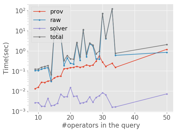
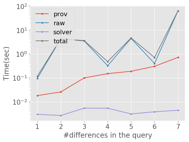
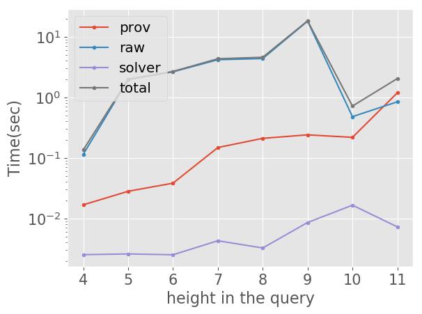
Figure 3. Query complexity vs. time, algorithm=$Opt_{\sigma}$, #tuples=100k; raw is for evaluating queries $Q_{1}-Q_{2}$; prov-sp is for provenance queries with selection on one tuple; solver-opt is for finding the smallest witness with Z3 SMT optimizer; total is the total running time of $Opt_{\sigma}$.

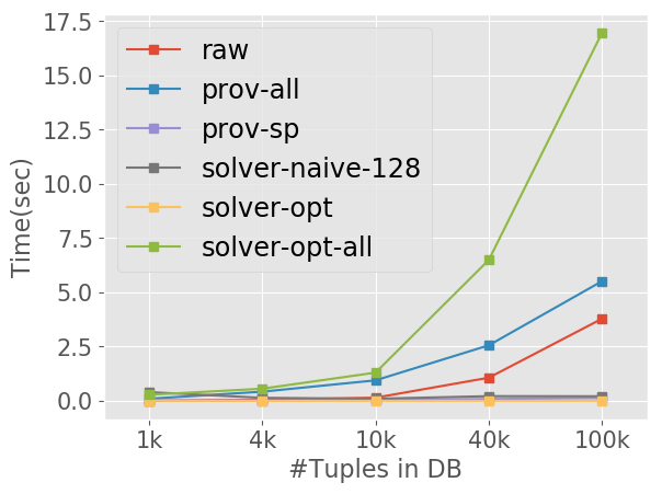
Figure 4. Average Running Time of Each Component.

Figure 5. (a) Witness size vs. solver strategies and Queries, #tuples=100K; (b) Witness size vs. solver strategies and runtime, #tuples = 100K

Solver strategy vs. witness size. Since our goal is to find the smallest witness, the metric for evaluating the quality of the witnesses as explanations is the size. We experiment different constraint-solving strategies: Naive-* is to use the Z3 SMT solver to get satisfying models to the Boolean formula of how-provenance, until there are no more satisfying models or it finishes enumerating M different models (we chose M=128); Opt is to use Z3 SMT optimizer to directly find the model with least number of variables set to true. Naive-* is not satisfying because there is no guarantee on the model size it finds. Figure 5 summarizes the results. Since the SAT solver used by Naive-* can return an arbitrary model every time, we repeat each experiment with Naive-* 10 times and report the average minimum witness size found among the 10 repetitions. Opt always return a smaller witness compared to Naive-*, while the runtime overhead compared to even Naive-1 is negligible. Of course, performance of these approaches heavily depends on the solver implementation; a comprehensive evaluation would be beyond the scope of this paper. Here, we simply observe that our implementation of Opt provides good performance and solution quality in practice, as it cannot be easily beaten by simply enumerating a number of models.

7.2. Synthetic Aggregate Queries

We experimented on the TPC-H benchmark database generated at scale 1 on queries Q4, Q16, Q18, Q21, and a modified Q21-S with an additional selection on aggregate value at the top of the query tree. We choose these queries because they do not involve arithmetic operations on aggregate functions. First we dropped the ORDER BY operator and rewrote these queries using the relational algebra interpreter, then we experimented both the provenance for aggregate queries approach (Agg-Basic) and the heuristic approach (Agg-Opt) discussed in Section 5. We also experimented provenance for aggregate queries approach with parameterization (Agg-Param) on Q18 (it has a selection predicate with aggregate value). We intentionally made two wrong queries for each query, of which the errors include different selection conditions, incorrect use of difference, and incorrect position of projection. These are common errors in the students queries from the previous experiment.

Query	Agg-Basic			Agg-Opt
	Raw Query Eval. Time	Prov. Query Eval. Time	Solver Runtime	Raw Query Eval. Time	Prov. Query Eval. Time	Solver Runtime
Q4	3.6036	4.0403	timeout	2.1382	0.0029	0.0151
Q16	0.8676	0.1349	0.2471	0.7618	0.1084	0.0022
Q18	6.8751	0.0086	0.0134	14.2513	0.0130	0.0039
Q21	21.5184	2.6205	31.1106	21.8072	0.0577	0.0066
Q21-S	21.5408	2.8034	155.6828	22.1634	0.0524	0.0061

Figure 6. Computation time (sec.), for the TPC-H benchmark, scale=1, timeout = not finishing after 2 hours

	Solver Runtime (sec.)	Size of Counterexample
Agg-Basic	0.0134	25.3
Agg-Param	0.0210	7.5

Figure 7. Effectiveness of algorithm with parameterization, on TPC-H Q18, scale-factor = 1

Figure 7 includes the runtime of our algorithms to find the smallest counterexample for each TPC-H query we experiment. We present a breakdown of the execution time of our solutions: raw query evaluation time, provenance query evaluation time, SMT-solver running time. We find that the heuristic algorithm performs well for queries where the aggregation operators are at the top of the query tree. While the performance of the provenance for aggregate query algorithm decreases as the database size increases, and is significantly affected by the number of tuples in the group (The SMT solver does not scale well).

For Q18, since it involves an aggregate predicate, we experiment the effectiveness of the algorithm with parameterization. Figure 7 shows the solver runtime and the size of the counterexample of the provenance for aggregate query algorithm with/without parameterization. The size of the counterexample is reduced by 70% while the runtime only increases from 0.0134 seconds to 0.0210 seconds.

8. User Study

Since one motivation of our work is to provide small examples as explanations of why queries are incorrect, we built our RATest as a web-based teaching tool and deployed in an undergraduate database class in a US university in Fall 2018 with about 170 students. For one homework assignment, students needed to write relational algebra queries to answer 10 questions against a database of six tables about bars, beers, drinkers, and their relationships. The difficulties of these 10 problems range from simple to very difficult. The students had a small sample database instance to try their queries on. Their submissions were tested by an auto-grader against a large, hidden database instance designed to exercise more corner cases and catch more errors; if these answers differed from those returned by the correct queries (also hidden), the students would see the failed tests with some addition information about the error (but not the hidden database instance or the correct queries). The final submissions were then graded manually informed by the auto-grader results; partial credits were given. For the purpose of this user study, we normalize the student score for each question to $[0,100]$.

We did not wish to create unfair advantages for or undue burdens on students with our user study. This consideration constrained our user study design. For example, we ruled out the option of dividing students into groups where only some of them benefit from RATest; we also ruled out creating additional homework problems without counting them towards the course grades. Therefore, we made the use of RATest completely optional (and with no extra incentives other than the help RATest offers itself). RATest was given the correct queries and the same database instance used by the auto-grader for testing. If a student query returned an incorrect result, RATest would show a small database instance (a subset of the hidden one), together with the results of the incorrect query and the hidden correct query on this small instance. We made RATest available for only 5 out of the 10 problems. Leaving some problems out allowed us to study the same student’s performance on different problems might be influence by the use of RATest. The 5 problems were chosen to cover the entire range of difficulties:

• Find drinkers who frequent any bar serving Corona.

• Find drinkers who frequent both JJ Pub and Satisfaction.

• Find bars frequented by either Ben or Dan, but not both.

• For each bar, find the drinker who frequents it the greatest number of times.

• Find all drinkers who frequent only those bars that serve some beers they like.

Students must use basic relational algebra; in particular, they were not allowed to use aggregation. Problems (g) and (i) are more challenging than others: (g) involves non-trivial uses of self-join and difference; (i) involves two uses of difference.

We released RATest a week in advance of the homework due date. We collected usage patterns on RATest, as well as how students eventually scored on the homework problems. Ideally, we wanted to answer the following questions: i) Did students who used RATest do better than those who didn’t? ii) For students who used RATest, how did they do on problems with and without RATest’s help? We should note upfront that we expected no simple answers to these questions, as scores could be impacted by a variety of factors, including the inherent difficulty of a question itself, individual students’ abilities and motivation, as well as the learning effect (where one gets better at writing queries in general after more exercises). Therefore, to supplement quantitative analysis of usage patterns and scores, we also gave an optional, anonymous questionnaire to all students after the homework due date.

Problem	# of users		average # of attempts
	total	who got a correct answer eventually	over all users	before a correct answer
(b)	102	93	4.08	1.79
(d)	93	93	3.12	1.57
(e)	100	95	5.24	3.45
(g)	99	91	5.90	3.76
(i)	120	94	11.10	7.46

Figure 8. Statistics on RATest usage.

Did the student use	No	Yes	Time of the first use (before due date)
RATest for (i)?			5-7 days	3-4 days	2 days	1 day
# of students	49	120	45	30	16	29
Mean score on (i)	89.80	94.40	97.14	99.05	91.96	86.70
Std. dev.	30.58	19.00	15.41	5.22	25.54	26.16
Mean score on (h)	88.34	93.57	96.83	95.24	95.54	85.71
Std. dev.	31.77	20.86	14.89	18.12	17.86	30.06
Mean score on (j)	85.46	85.42	96.67	90.00	82.81	64.66
Std. dev.	34.17	34.39	16.51	30.51	37.33	47.02

Figure 9. Comparison of performance on (h) and (j) between students whether they used RATest for (i) or not.

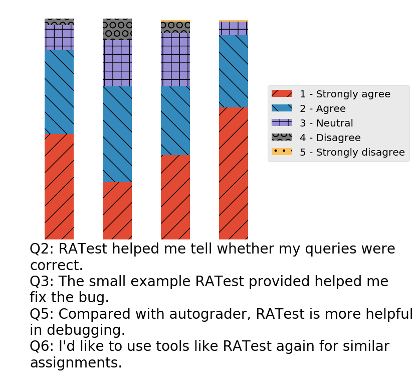
Figure 10. Results of student feedback.

Did the student use RATest?		No	Yes
Problem (b)	# of students	67	102
	Mean score	100.00	100.00
	Std. dev.	0.00	0.00
Problem (d)	# of students	76	93
	Mean score	100.00	100.00
	Std. dev.	0.00	0.00
Problem (e)	# of students	69	100
	Mean score	99.03	99.67
	Std. dev.	5.63	3.33
Problem (g)	# of students	70	99
	Mean score	92.38	97.98
	Std. dev.	26.11	14.14
Problem (i)	# of students	49	120
	Mean score	89.80	94.40
	Std. dev.	30.58	19.00

Table 5. Comparison of performance between students who did not use RATest and those who did, on problems for which RATest was available.

Quantitative Analysis of Usage Patterns and Scores.  Before exploring the impact of RATest on student scores, let us examine some basic usage statistics, summarized in Figure 10. Overall, $137$ students (more than $80\%$ of the class) attempted a total of $3{,}146$ submissions to RATest. The sheer volume of the usage speaks to the demand for tools like RATest, and the sustained usage (across problems) suggests that the students found RATest useful. It is also worth noting that number of attempts reflects problem difficulty; for example, (i), the most difficult problem, took far more attempts than other problems. We also note that while RATest helped the vast of majority of its users get the correct queries in the end; some users never did. We observed in the usage log some unintended uses of RATest: e.g., one student made more than a hundred incorrect attempts on a problem, most of which contained basic errors (such as syntax); apparently, RATest was used to just try queries out as opposed to debugging queries after they failed the auto-grader. Such outliers explain the phenomenon shown in Figure 10 where the overall average # of attempts were much higher than the average # before a correct attempt.

Next, we examine how the use of RATest helps improve student scores. Table 5 compares the scores achieved by students who did not use RATest versus those who did, on problem for which we made RATest available. For simple problems such as (b), (d), and (e), there is no little or no difference at all, because nearly everybody got perfect scores with or without help from RATest. However, for more difficult problems, (g) and (i), students who used RATest had a clear advantage, with average scores improved from 92.38 to 97.98 and from 89.80 to 94.40, respectively. Of course, within the constraints of our user study, it is still difficult to conclude how much of this improvement comes from RATest itself; it is conceivable that students who opted to use RATest were simply more diligent and therefore would generally perform better than others. While we cannot definitively attribute all improvement in student performance to RATest, we next provide some evidence that it did help in a significant way.

Here, we zoom in on the three most difficult problems, (h), (i), and (j); RATest was only made available for (i). Problem (h) (find all drinkers who frequent only those bars that serve some beers they like) is quite similar to (i) (the difference being “some beers” vs. “only beers”). Problem (j) (find all (bar1, bar2) pairs where the set of beer served at bar1 is a proper subset of those served at bar2) on other hand requires very different solution strategy. Between those who did not use RATest for (i) and those who did, Figure 10 (focus on the first three columns and ignore the rest for now) compares their scores on (h) and (j). We see that for the similar problem (h), those who used RATest on (i) significantly improved their scores on (h), with a degree comparable to the improvement on (i). For the dissimilar problem (j), those who used RATest no (i) showed no improvement in their scores on (j)—the two score distributions are practically the same. We make two observations here. First, it is clear that not all improvement in student performance can be explained by student “diligence” alone; otherwise we would have seen higher performance on (j) for students who used RATest on (i). Second, there is clearly a learning effect: using RATest for one problem can help with a similar problem: (i) helps (h).

Figure 10, in its last four columns, also breaks down the statistics by when a student started to work on Problem (i). Not surprisingly, we see that “procrastinators” (those who started very close to the due date) performed clearly worse than others. If somebody started to work on (i) using RATest only the day before the homework was due, this individual would be expected to perform even worse than an “average” student who opted not to use RATest at all, especially for the last problem. It would have been nice if we can similarly break down the statistics for students who opted not to use RATest at all, but it was not possible in that case to know when they started to work on the problems. We could only conjecture that a similar trend might exist for procrastinators, so using RATest did not hurt any individual’s performance.

Results of Anonymous Questionnaire.  We collected 134 valid responses to our anonymous questionnaire; Figure 10 summarizes these responses. The feedback was largely positive. For instance, 69.4% of the respondents agree or strongly agree that the explanation by counterexamples helped them understand or fix the bug in their queries, and 93.2% would like to use similar tools in the future for assignments on querying databases. We also asked students which problems they found RATest to be most helpful (multiple choices were allowed): 58% voted for (g) and 94% voted for (i), which were indeed the most challenging ones. We also solicited open-ended comments on RATest. These comments were overwhelming positive and reinforces our conclusions from the quantitative analysis, e.g.:

• “It was incredibly useful debugging edge cases in the larger dataset not provided in our sample dataset with behavior not explicitly described in the problem set.”

• “Overall, very helpful and would like to see similar testers for future assignments.”

• “I liked how it gave us a concise example showing what we did wrong.”

Summary.  Overall, the conclusion of our user study is positive. Students who used RATest did better, and their improvement cannot be attributed all to merely the fact that they opted to use an additional tool—RATest did add real value. Also, using RATest on one problem could also help with another problem, provided that the problems are similar. Finally, most students found RATest very useful and would like to use similar systems in the future.

9. Related Work

Test data generation.  Cosette(Chu et al., 2017), which targets at deciding SQL equivalence without any test instances, encodes SQL queries to constraints using symbolic execution, and uses a constraint solver to find counterexamples over which the two queries return different results. Cosette uses incremental solving to dynamically increase the size of each symbolic relation, thus it will return counterexamples with least number of distinct tuples, but the total number of tuples is not minimized. ALso, it deals with only integer domain and returns counterexamples of arbitary values, which may be hard for people to read. XData(Chandra et al., 2015) generates test data by covering different types of query mutants of the standard query, without looking into wrong queries. Qex(Veanes et al., 2010) is a tool for generating input relations and parameter values for a parameterized SQL query that also uses the SMT solver Z3, which aims at unit testing of SQL queries. It does not support nested queries and set operations and hence it cannot work for our problem because of our use of difference.

Provenance and witness.  Data provenance has primarily been studied for non-aggregate queries: Buneman et al.(Buneman et al., 2001) defined why-provenance of an output tuple in the result set, which they call the witness basis. Green et al.(Green et al., 2007a) introduced how-provenance with the general framework of provenance semiring. Sarma et al.(Sarma et al., 2008) gave algorithms for computing how-provenance over various RA operators in the Trio system. Amsterdamer et al. (Amsterdamer et al., 2011b) extended the provenance semiring framework(Green et al., 2007a) to support aggregate queries. Besides these theoretical works, there are systems that capture different forms of provenance (Karvounarakis et al., 2010; Glavic and Alonso, 2009; Arab et al., 2014; Green et al., 2007b; Psallidas and Wu, 2018; Senellart et al., 2018). However, to the best of our knowledge, no prior work considered SWP/SCP, and there are no systems available that support provenance for general SPJUD and aggregate queries.

Teaching or grading tool for programming.  Due to popularity of students taking programming-related courses, teaching and grading tools for programming assignments that automatically generate feedback for submissions are receiving a lot of attention(Parihar et al., 2017; Kaleeswaran et al., 2016; Gupta et al., 2017). In the database community, Chandra et al. built XData(Chandra et al., 2015) that can be used for grading by generating multiple test cases for different query mutants, as well as giving immediate feedback to student. The latter is similar to our RATest tool. Jiang and Nandi(Jiang and Nandi, 2015; Nandi, 2015) designed and prototyped interactive electronic textbook to help students get rapid feedbacks from querying the database with novel interaction techniques.

Explanations for query answers.  Explanations based on tuples in the provenance has been recently studied by Wu-Madden (Wu and Madden, 2013) and Roy-Suciu (Roy and Suciu, 2014). These works take an aggregate query and a user question as input, find tuples whose removal will change the answer in the opposite direction, and returns a compact summary as explanations.

Appendix A Proofs of Theorems in Section 3

We will give the proofs of theorems in Table 1 in this section.

A.1. SJ and SPU Queries

Given $t\in Q_{1}(D)\setminus Q_{2}(D)$, the poly-time algorithm for SJ and SPU queries involve finding a smallest witness of $t$ in $D$ for $Q_{1}$, and using the fact that $Q_{2}$ is monotone and $t\notin Q_{2}(D)$, $\forall D^{\prime}\subseteq D$, $t\notin Q_{2}(D^{\prime})$.

Theorem 1.

The SWP for two SJ queries is poly-time solvable in combined complexity.

Proof.

Let $R_{1},...,R_{k}$ be all the relations that participate in the SJ query $Q_{1}$. For each relation $R_{i}$, $i\in[1,k]$, there must exist exactly one tuple $t_{i}=t.R_{i}$ (the $R_{i}$ component of $t$), which is part of the witness of $t$ (under set semantic). Since each $t_{i}$ must satisfy all selection conditions for $t$ to appear in $Q_{1}(D)$, the set $D_{t}=\{t_{i}|i\in[1,k]\}$ ensures that $t\in Q_{1}(D_{t})$, and must be minimal. Since $Q_{2}$ is monotone and $t\notin Q_{2}(D)$, we have $t\notin Q_{2}(D_{t})$; hence $t\in(Q_{2}-Q_{1})(D_{t})$. The running time to find $D_{t}$ is polynomial in $k$, giving polynomial combined complexity. ∎

When projection is allowed, an output tuple may have multiple minimal witnesses, and we pick any one of them.

Theorem 2.

The SWP for two SPU queries is polynomial-time solvable in combined complexity.

Proof.

We first consider SP queries. Given an output tuple $t$ in $Q_{1}(D)$, we scan the input relation to find a tuple $t^{\prime}$ that satisfies the selection condition and whose projected attributes equal to $t$. The smallest witness $D_{t}$ only consists of only $t^{\prime}$. For SPU queries, we do the same procedure as SP queries. At least one relation will return $t^{\prime}$. Since $Q_{2}$ is monotone and $t\notin Q_{2}(D)$, we have $t\notin Q_{2}(D_{t})$. The running time to find $D_{t}=\{t^{\prime}\}$ is polynomial in $k$. ∎

A.2. PJ Queries

For queries involving both projection and join, we show that it is NP-hard in query complexity to find the smallest witness, even when the query can be evaluated in poly-time.

Theorem 3.

The SWP for two PJ queries is NP-hard in query complexity.

Proof.

We prove the theorem by a reduction from the vertex cover problem with vertex degree at most 3, which is known to be NP-complete (Garey et al., 1976) and is defined as follows: Given an undirected graph $G(V,E)$ with vertex set $V$ and edge set $E$, where the degree of every vertex is at most 3, decide whether there exists a vertex cover $C$ of at most $p$ vertices such that each edge in $E$ is adjacent to at least one vertex in the set.

Construction.  Given $G(V,E)$, suppose $V=\{v_{1},...,v_{n}\}$, and $E=\{e_{1},\cdots,e_{m}\}$. We encode each vertex as a tuple in the relation $R(A,Z,E_{1},E_{2},E_{3})$. For each vertex $v_{i}\in V$, $R$ contains a tuple $t_{i}=(v_{i},z,e_{i1},e_{i2},e_{i3})$, where $e_{i_{1}},e_{i_{2}},e_{i_{3}}$ are identifiers of edges adjacent to $v_{i}$, $i_{1}<i_{2}<i_{3}$. If the degree of $v_{i}$ is less than 3, the identifiers are replaced by a null symbol “$*$”. The attribute $Z=z$ is a constant for all tuples. In addition to $R$, we have $m$ relations $S_{1},...,S_{m}$. Each $S_{i}$, $i\in[1,m]$, has schema $S_{i}(E,Z)$. For the edge $e_{i}\in E$, $S_{i}$ contains a single tuple $(e_{i},z)$. Let $D=(R,S_{1},...,S_{m})$ be the database instance.

Next, we construct $Q_{1}$ involving $PJ$ that consist of $m$ subqueries as follows: For all $i\in[1,m]$, let $q_{i}=$
$\pi_{Z}(R$ $\Join_{R.E_{1}=S_{i}.E\lor R.E_{2}=S_{i}.E\lor R.E_{3}=S_{i}.E}S_{i})$, which operates on $S_{i}$ and $R$, checks for match of $R.E_{1},R.E_{2}$, or $R.E_{3}$ with $S_{i}.E$, and then projects on to $Z$. Then we construct $Q_{1}$ = $q_{1}\Join q_{2}\Join...\Join q_{m}]$ using natural join on $Z$. All queries $q_{i}$ and $Q_{1}$ have a single attribute $Z$. Note that, initially, $q_{i}(D)=\{(z)\}$ for all $i\in[1,m]$, and therefore $Q_{1}(D)=\{(z)\}$ as well. The query $Q_{2}$ also outputs the attribute $Z$, but not the tuple $\{(z)\}$. We set $Q_{2}=\pi_{Z}(R\Join_{R.Z\neq S_{1}.Z}S_{1})$ (the choice of $S_{1}$ is arbitrary), and therefore $Q_{2}(D)=\{\}$ is empty. The tuple $t$ for which we want to find the smallest witness in $(Q_{1}-Q_{2})(D)$ is $(z)$. In other words, the goal is to find a subinstance $D^{\prime}=(R^{\prime},S^{\prime}_{1},...,S^{\prime}_{m}),$ $R^{\prime}\subseteq R,S^{\prime}_{1}\subseteq S_{1},...,S^{\prime}_{m}\subseteq S_{m}$, such that $(z)\in Q_{1}(D)\setminus Q_{2}(D)$.

Below we argue that $G$ has a vertex cover of size $\leq p$, if and only if the SWP instance above has a witness $D^{\prime}$ of size $\leq p+m$ where $m$ is the number of edges in $G$.

The “Only If” direction.  Suppose we are given a vertex cover $C$ with at most $p$ vertices in $G$. We construct $R_{i}^{\prime}=\{t_{j}~{}|~{}v_{j}\in C\}$, and $S_{i}^{\prime}=S_{i}$ for all $i\in[1,m]$. Since $|C|\leq p$, $|D^{\prime}|\leq p+m$ since each $S_{i}$ contains a single tuple. Since $C$ is a vertex cover, for all edge $e_{i}=(v_{j},v_{\ell})\in E$, either $v_{j}\in C$ or $v_{\ell}\in C$. Suppose without loss of generality $v_{j}\in C$. Then (wlog.) assume $t_{j}=(v_{j},z,e_{i},e^{\prime},e^{\prime\prime})$ where $e^{\prime},e^{\prime\prime}$ are other two adjacent edges on $v_{j}$ (they could be $*$ as well if the degree of $v_{j}$ is $<3$). The tuple $t_{j}$ and the tuple $S_{i}(e_{i},z)$ will satisfy the join condition of $q_{i}$ (irrespective of the position of $e_{i}$ in $t_{i}$), and the projection will output $(z)$. Since $C$ is a vertex cover, for all $i\in[1,m]$, $q_{i}(D^{\prime})=\{(z)\}$. Therefore, $Q_{1}(D^{\prime})=\{(z)\}$. $Q_{2}(D^{\prime})$ remains empty. Hence $(z)\in Q_{1}(D^{\prime})\setminus Q_{2}(D^{\prime})$ Therefore, $D^{\prime}$ is a witness of $(z)$ of size at most $p+m$.

The “If” direction.  For the opposite direction, consider a witness $D^{\prime}=(R^{\prime},S^{\prime}_{1},...,S^{\prime}_{m})$ where $R^{\prime}\subseteq R,S^{\prime}_{1}\subseteq S_{1},...,S^{\prime}_{m}\subseteq S_{m},|R^{\prime}|+|S^{\prime}_{1}|+...+|S^{\prime}_{m}|\leq p+m$, such that $(z)\in Q_{1}(D^{\prime})\setminus Q_{2}(D^{\prime})$, i.e., $(z)\in Q_{1}(D^{\prime})$. We construct $C=\{v_{i}~{}|~{}t_{i}\in R^{\prime}\}$. Note that if $(z)\in Q_{1}(D^{\prime})$, $(z)$ must be in the result of all subqueries $q_{i}(D^{\prime})$, $i\in[1,m]$. And $q_{i}(D^{\prime})$ returns $(z)$ if and only if (a) $S^{\prime}_{i}$ is not empty (i.e., $S_{i}^{\prime}=S_{i}$ since $S_{i}$ had only one tuple), and (b) if $e_{i}=(v_{j},v_{\ell})$, at least one of $t_{j}$ or $t_{\ell}$ must appear in $R^{\prime}$ to satisfy the join condition in $q_{i}$; otherwise $q_{i}$ returns an empty result and thus $Q_{1}$ returns an empty result. Therefore, all $S^{\prime}_{i}$ must be equal to $S_{i}$, $|S^{\prime}_{i}|=1$. Then we have $|S^{\prime}_{1}|+...+|S^{\prime}_{m}|=m$. Since $|D^{\prime}|\leq p+m$, $|R^{\prime}|\leq p$, and thus we get a vertex cover $C$ of size at most $p$.

An example reduction is shown in Figure 11. ∎

(a) $G(V,E)$

$E$	$Z$
$e_{1}$	$z$

… $E$ $Z$ $e_{7}$ $z$

(b) $S_{1},\cdots,S_{7}$

$A$	$Z$	$E_{1}$	$E_{2}$	$E_{3}$
$v_{1}$	$z$	$e_{1}$	$e_{6}$	$*$
$v_{2}$	$z$	$e_{1}$	$e_{2}$	$e_{7}$
$v_{3}$	$z$	$e_{2}$	$e_{3}$	$*$
$v_{4}$	$z$	$e_{4}$	$e_{6}$	$e_{7}$
$v_{5}$	$z$	$e_{3}$	$e_{4}$	$e_{5}$
$v_{6}$	$z$	$e_{5}$	$*$	$*$

(c) R

Figure 11. Example reduction in Theorem 3

A.3. JU Queries

Theorem 4.

The SWP for two JU queries is NP-hard in query complexity.

Proof.

We reduce from the vertex cover problem.

Construction.  Suppose $V=\{v_{1},...,v_{n}\}$ and $E=\{e_{1},\cdots,$
$e_{m}\}$. For each vertex $v_{i}$ in $G$, there is a relation $R_{i}(Z)$ which consists of a single tuple $(z)$. For each edge $e_{i}=(v_{j},v_{\ell})\in E$, we construct a query $q_{i}=R_{j}\cup R_{\ell}$. Then we construct a query $Q_{1}=q_{1}\Join\cdots\Join q_{m}$, where the join is a natural join on $Z$. We construct $Q_{2}=R_{1}\Join_{R_{1}.Z\neq R_{2}.Z}R_{2}$ (the choice of $R_{1},R_{2}$ is arbitrary). Hence $D=(R_{1},\cdots,R_{n})$, $Q_{1}(D)=\{(z)\}$, and $Q_{2}(D)=\{\}$. The output tuple $(z)\in Q_{1}(D)\setminus Q_{2}(D)$, and the goal is to find a witness $D^{\prime}=$ $(R_{1}^{\prime},\cdots,$
$R_{n}^{\prime})$ for $(z)$ where $R_{i}^{\prime}\subseteq R_{i}$ for all $i\in[1,n]$.

We show that there exists a vertex cover $C$ in $G$ of size $\leq p$ if and only if there is a witness $D^{\prime}$ for $(z)$ of size $\leq p$.

The “Only If” direction.  Consider a vertex cover $C$ of $G$ such that $|C|\leq p$. If $v_{i}\in C$, then $R_{i}^{\prime}=\{(z)\}$, otherwise $R^{\prime}_{i}=\{\}$. Since $C$ is a vertex cover, all edges must be covered. For an edge $e_{i}=(v_{j},v_{\ell})$, suppose wlog. $v_{j}\in C$. Hence the subquery $q_{i}=R_{j}\cup R_{\ell}$ returns $(z)$ on $D^{\prime}$. Therefore, $Q_{1}(D^{\prime})=(z),Q_{2}(D^{\prime})=\{\}$, $(z)\in Q_{1}(D^{\prime})\setminus Q_{2}(D^{\prime})$, i.e., $D^{\prime}$ is a witness for $(z)$, and $|D^{\prime}|=|C|\leq p$.

The “If” direction.  Consider any witness $D^{\prime}=(R^{\prime}_{1},...,R^{\prime}_{n})$ where $R^{\prime}_{1}\subseteq R_{1},...,R^{\prime}_{n}\subseteq R_{n}$ and $|R^{\prime}_{1}|+...+|R^{\prime}_{n}|\leq p$, such that $(z)\in Q_{1}(D^{\prime})\setminus Q_{2}(D^{\prime})$, i.e., $(z)\in Q_{1}(D^{\prime})$. Since $R_{i}$ had only one tuple $(z)$, either $R^{\prime}_{i}$ has $(z)$ or it is empty. If tuple $(z)\in R^{\prime}_{i}$, then we add vertex $v_{i}$ to a set $C$. If $(z)$ is in the result of $Q_{1}(D^{\prime})$, $(z)$ must be in the result of all subqueries $q_{i}(D^{\prime})$ for all $i\in[1,m]$. For $e_{i}=(v_{j},v_{\ell})$, $q_{i}(D^{\prime})$ returns $(z)$ if and only if at least one of $R^{\prime}_{j}$ and $R^{\prime}_{\ell}$ is not empty; otherwise $q_{i}$ returns an empty result and thus $Q_{1}$ returns an empty result. Therefore, for each edge $e_{i}\in E$, at least one of its adjacent vertices $v_{j}$ or $v_{\ell}$ must exist in $C$. Hence $C$ is a vertex cover, and $|C|=|D^{\prime}|\leq p$. ∎

On the other hand, the following theorem shows that if all unions appear after all joins (which we call JU^∗ queries), then the SWP can be solved in poly-time in combined complexity.

Theorem 5.

The SWP for two JU^∗ queries is polynomial time solvable in combined complexity.

Proof.

Let $t\in Q_{1}(D)\setminus Q_{2}(D)$. According to Theorem 1, the SWP for SJ queries is polynomial time solvable in combined complexity. Hence, we look for the smallest witness of $t$ in join-only part of $Q_{1}$, and choose the one with smallest number of tuples. The running time is polynomial in both $n=|D|$ and $k$. ∎

A.4. Size-Bounded SPJU Queries

Theorem 6 shows that if the SPJU queries are of bounded size (i.e. considering more standard data complexity), there is a polynomial time algorithm for SWP. We prove this theorem using Proposition A.1, which is intuitive and known (e.g., (Roy et al., 2011)). We use $m$-DNF to refer to a DNF where each minterm has at most $m$ literals.

Proposition A.1.

Given an SPJU query $Q$, a database instance $D$, and an output tuple $t\in Q(D)$, the how-provenance of $t$ in $Q(D)$ can be transformed into a $k+1$-DNF in polynomial time when $Q$ is of bounded size, where $k$ is the number of join operations in $Q$.

Theorem 6.

The SWP for two SPJU queries is polynomial-time solvable in data complexity.

Proof.

Let $t$ be an output tuple in $Q_{1}(D)\setminus Q_{2}(D)$. Since $Q_{2}$ is monotone, $t\notin Q_{2}(D^{\prime})$ for any $D^{\prime}\subseteq D$. According to Proposition A.1, we can compute the how-provenance ${\tt Prv}_{(Q_{1}-Q_{2})(D)}(t)$ in DNF in poly-time in data complexity. Then we scan the DNF to find the minterm with least number of literals, and this minterm represents the smallest witness for $t$ in $Q_{1}(D)-Q_{2}(D)$. The literals in this clause are the identifiers of tuples in the smallest witness. ∎

For instance, if ${\tt Prv}(t)=a+bc$, then $a$ forms the smallest witness.

A.5. Queries Involving Difference

Before discussing general SPJUD queries, let’s focus on one special class of SPJUD queries where all differences appear after all SPJU operators (which we call SPJUD^∗ queries). More formally, we define this class using formal grammar: $Q\rightarrow q^{+}|Q-Q$, where $q^{+}$ is a terminal that represents SPJU queries. For instance, queries $Q_{1}$ and $Q_{2}$ in Example 1 are SPJUD^∗ queries. The following theorem shows that the SWP can be solved in poly-time for SPJUD^∗ queries.

Theorem 7.

The SWP for two SPJUD^∗ queries is polynomial-time solvable in data complexity.

Proof.

Let $t$ be an output tuple in $Q_{1}(D)\setminus Q_{2}(D)$. Since $Q_{1}$ and $Q_{2}$ are SPJUD^∗ queries that can be written as nested differences of queries like $q_{1}-q_{2}-(q_{3}-(q_{4}-q_{5}))-...$, where all $q_{i}$-s are SPJU queries, $Q_{1}-Q_{2}$ is also an SPJUD^∗ query. The output tuple $t$ must be either in or not in the result of each $q_{i}$. We find the smallest witness by enumerating the minimal witnesses of $t$ w.r.t. every $q_{i}$ and $D$. If $t$ is in the result of $q_{i}(D)$, let $w_{i}$ be the set of minimal witnesses of $t$ w.r.t. $q_{i}$ and $D$. Then we pick one element from every $w_{i}\cup\{\emptyset\}$, and construct $w$ as the union of all witnesses or the empty set we picked. We evaluate $Q_{1}$ and $Q_{2}$ on $w$ to see whether it is a witness for $t$, and record the $w$ of the smallest size. We finish this procedure until we enumerate all combinations.

This procedure will return the smallest witness because: (i) if $t\notin q_{i}(D)$, $t$ will also not be in $q_{i}(w)$ for any $w\subseteq D$ due to monotonicity, so we don’t need to consider such $q_{i}$-s; (ii) Assume that $w^{\prime}$ is a smallest witness of $t$ w.r.t. $Q_{1}-Q_{2}$ and $D$, for all $q_{i}$ where $t\in q_{i}(w^{\prime})$, $w^{\prime}$ must be a superset of a minimal witness of $t$ w.r.t. $q_{i}$ and $D$. Hence $w^{\prime}$ must be the union of minimal witnesses of $t$ w.r.t. these $q_{i}$-s and $D$; otherwise, if $w^{\prime}$ is a strict superset of the union of minimal witnesses of $t$, we can always remove tuples not belong to any minimal witness of $t$ w.r.t. $q_{i}$-s and $D$ from $w^{\prime}$, without affecting $t$ to be in or not in any $q_{i}$, which contradicts the assumption that $w^{\prime}$ is a smallest witness. Therefore a smallest witness of $t$ w.r.t. $Q_{1}-Q_{2}$ and $D$ must be union of minimal witness of $t$ w.r.t. $q_{i}$ and $D$, and thus it must be enumerated during the enumeration procedure.

The time complexity of entire enumeration process is $O(\Pi_{i}m^{k_{i}})=O(m^{kd})$, where d is the number of difference operators, m is the max size of relations, k is the max complexity of each SPJU query $q_{i}$. When queries are of bounded sizes, i.e., fix d and k, the SWP for two SPJUD queries that can be written as nested differences of SPJU queries is polynomial-time solvable. ∎

SWP is NP-hard in general even for bounded-size queries.

Theorem 8.

The SWP for two SPJUD queries $Q_{1}$ and $Q_{2}$ is NP-hard in data complexity.

Proof.

We again give a reduction from the vertex cover problem with vertex degree at most 3 (see Theorem 3).

Construction.  Suppose in $G=(V,E)$, $V=\{v_{1},...,v_{n}\}$, $E=\{e_{1},\cdots,e_{m}\}$. We construct two relations $R(A,Z,E_{1},E_{2},E_{3})$ and $S(B,C,Z)$. For each vertex $v_{i}\in V$, $R$ contains a tuple $t_{i}=(v_{i},e_{i1},e_{i2},e_{i3},z)$, where $e_{i_{1}},e_{i_{2}},e_{i_{3}}$ are the identifiers of edges adjacent to $v_{i}$, $i_{1}<i_{2}<i_{3}$. If the degree of $v_{i}$ is less than 3, the identifiers are replaced by a null symbol “$*$”. Here $z$ is a constant. For each edge $e_{i}\in E$, $S$ contains a tuple $(e_{i},e_{(i\%m)+1},z,z)$, where $e_{(i\%m)+1}$ is the identifier of the next edge in the edge list (the next edge of $e_{m}$ is $e_{1}$). Let $D=(R,S)$ be the database instance.

Next, we construct an SPJUD query that consists of several subqueries as follows: Let $q_{1}$ (on $S$) = $\pi_{Z}(S)$; $q_{2}$ (on $S$) $=\pi_{B,Z}(S)$; $q_{3}$ (on $R,S$)=$\pi_{S.C,S.Z}(S\Join_{S.C=E_{1}\lor S.C=E_{2}\lor S.C=E_{3}}R)$. Then we construct $Q_{1}=q_{1}$, hence $Q_{1}(D)=\{(z)\}$. We also construct $Q_{2}=\pi_{Z}(q_{2}\setminus q_{3})$ (assume $C$ in $q_{3}$ is renamed to $B$). For edge $e_{i}=(v_{j},v_{\ell})$, the edge $e_{i}$ appears for both tuples $t_{j},t_{\ell}$ (in one of $E_{1},E_{2},E_{3}$ attributes), and therefore, $(e_{i},z)$ appears in the result of $q_{3}(D)$ for every $i\in[1,m]$. Hence $q_{3}(D)=\pi_{B,Z}(S)$. So $q_{2}(D)\setminus q_{3}(D)=\emptyset$. Then $(Q_{1}-Q_{2})(D)=\{(z)\}$, and the goal is to find the smallest witness for $(z)$. For the vertex cover instance in Figure 11(a), $R$ will be as given in Figures 11(c), and $S$ will contain tuples $\{(e_{1},e_{2},z),(e_{2},e_{3},z),\cdots(e_{7},e_{1},z)\}$.

We now show that there exists a vertex cover $C$ of size at most $p$ in the graph $G$ if and only if there is a witness $D^{\prime}=(R^{\prime},S^{\prime})$ where $|R^{\prime}|+|S^{\prime}|\leq p+m$.

The “Only If” direction.  Suppose we are given a vertex cover $C$ of $G$ with at most $k$ vertices. Construct $R^{\prime}\{t_{i}~{}|~{}v_{i}\in C\}$, and $S^{\prime}=S$. $Q_{1}(D)=Q_{1}(D^{\prime})=\{(z)\}$ since $S$ is unchanged. Similarly, $q_{2}(D^{\prime})=\pi_{B,Z}(S))$ is unchanged. Since $C$ is a vertex cover, for every edge $e_{i}=(v_{j},v_{\ell})$ either $t_{i}$ or $t_{\ell}$ is in $R^{\prime}$, and hence $q_{3}(D^{\prime})=q_{3}(D)$, i.e., each $(e_{i},z)$, $i\in[1,m]$ appears in $q_{3}(D^{\prime})$. Hence $Q_{1}-Q_{2}$ will output tuple $(z)$ on $D^{\prime}$, $|R^{\prime}|=|C|\leq p,|S^{\prime}|=|S|=m$, and we get a witness of at most $p+m$ tuples.

The “If” direction.  Consider any witness $D^{\prime}=(R^{\prime},S^{\prime})$ where $R^{\prime}\subseteq R,S^{\prime}\subseteq S,|R^{\prime}|+|S^{\prime}|\leq p+m$, such that $(z)\in Q_{1}(D^{\prime})\setminus Q_{2}(D^{\prime})$. We construct $C=\{v_{i}~{}|~{}t_{i}\in R^{\prime}\}$. Since $(z)$ is in $Q_{1}(D^{\prime})\setminus Q_{2}(D^{\prime})$, $(z)$ must be in the result of $q_{1}(S^{\prime})$, and not in the result of $q_{2}(S^{\prime})-q_{3}(R^{\prime},S^{\prime})$, hence $S^{\prime}$ must contain at least one tuple. Therefore, $q_{2}(S^{\prime})$ outputs at least one tuple $(e_{i},z)$ since $S^{\prime}$ is not empty. In turn, $q_{3}(R^{\prime},S^{\prime})$ must output all tuples in $q_{2}(S^{\prime})$ to make $q_{2}(S^{\prime})-q_{3}(R^{\prime},S^{\prime})$ empty. (a) We argue that $S^{\prime}=S$. Suppose $S^{\prime}$ contains at least one tuple, say wlog, $(e_{1},e_{2},z)$. Then to remove $(e_{1},z)$ from $q_{2}(S^{\prime})\setminus q_{3}(R^{\prime},S^{\prime})$, $q_{3}(R^{\prime},S^{\prime})$ must contain $(e_{1},z)$, which can generate only from $S(e_{m},e_{1},z)$. Hence $(e_{m},e_{1},z)\in S^{\prime}$. In turn, $(e_{m},z)\in q_{2}(S^{\prime})$. To remove it, we need $S(e_{m-1},e_{m},z)$ in $S^{\prime}$. Continuing this argument (by induction), we get $S=S^{\prime}$. (b) Consider any tuple, say wlog., $(e_{1},e_{2},z)$ in $S^{\prime}$. Then to remove $(e_{1},z)$ from $q_{2}(S^{\prime})\setminus q_{3}(R^{\prime},S^{\prime})$, not only the tuple $(e_{m},e_{1},z)\in S^{\prime}$, it also has to satisfy the join condition with $R$. This will hold only if for one of the end points $v_{j},v_{\ell}$ of $e_{1}=(v_{j},v_{\ell})$, $t_{j}\in R^{\prime}$ or $t_{\ell}\in R^{\prime}$. This should hold for all edges, and therefore the set $C$ we constructed is a vertex cover. Since $|S^{\prime}|=|S|=m$, $|R^{\prime}|=|C|\leq p$, therefore, we get a vertex cover in $G$ of size at most $p$.

The queries we constructed during the reduction are all of bounded size, therefore the SWP for two SPJUD queries is NP-hard in data complexity even for queries of bounded size. ∎

References

- (1)
- Amsterdamer et al. (2011a) Yael Amsterdamer, Daniel Deutch, and Val Tannen. 2011a. On the Limitations of Provenance for Queries with Difference. In TaPP.
- Amsterdamer et al. (2011b) Yael Amsterdamer, Daniel Deutch, and Val Tannen. 2011b. Provenance for aggregate queries. In PODS. 153–164.
- Anonymous (2017) Anonymous. 2017. A Relational Algebra Interpreter. (2017).
- Arab et al. (2014) Bahareh Arab, Dieter Gawlick, Venkatesh Radhakrishnan, Hao Guo, and Boris Glavic. 2014. A generic provenance middleware for database queries, updates, and transactions. In TaPP.
- Barrett et al. (2011) Clark Barrett, Christopher L. Conway, Morgan Deters, et al. 2011. CVC4. In CAV ’11, Vol. 6806. Springer, 171–177.
- Barrett et al. (2010) Clark Barrett, Aaron Stump, Cesare Tinelli, et al. 2010. The smt-lib standard: Version 2.0. In Proceedings of the 8th International Workshop on Satisfiability Modulo Theories, Vol. 13. 14.
- Barrett and Tinelli (2018) Clark Barrett and Cesare Tinelli. 2018. Satisfiability modulo theories. In Handbook of Model Checking. Springer, 305–343.
- Biere ([n. d.]) Armin Biere. [n. d.]. CaDiCaL: Simplified Satisfiability Solver. https://github.com/arminbiere/cadical. ([n. d.]). [Online; accessed 24-Oct-2018].
- Bjørner et al. (2015) Nikolaj Bjørner, Anh-Dung Phan, and Lars Fleckenstein. 2015. Z-an optimizing SMT solver. In International Conference on Tools and Algorithms for the Construction and Analysis of Systems. Springer, 194–199.
- Buneman et al. (2001) Peter Buneman, Sanjeev Khanna, and Tan Wang-Chiew. 2001. Why and where: A characterization of data provenance. In International conference on database theory. Springer, 316–330.
- Chandra et al. (2015) Bikash Chandra, Bhupesh Chawda, Biplab Kar, KV Maheshwara Reddy, Shetal Shah, and S Sudarshan. 2015. Data generation for testing and grading SQL queries. The VLDB Journal 24, 6 (2015), 731–755.
- Chu et al. (2017) Shumo Chu, Chenglong Wang, Konstantin Weitz, and Alvin Cheung. 2017. Cosette: An Automated Prover for SQL.. In CIDR.
- Cohen et al. (2005) Sara Cohen, Yehoshua Sagiv, and Werner Nutt. 2005. Equivalences among aggregate queries with negation. ACM Transactions on Computational Logic (TOCL) 6, 2 (2005), 328–360.
- Council (2008) Transaction Processing Performance Council. 2008. TPC-H benchmark specification. Published at http://www.tcp.org/hspec.html 21 (2008), 592–603.
- De Moura and Bjørner (2008) Leonardo De Moura and Nikolaj Bjørner. 2008. Z3: An efficient SMT solver. In International conference on Tools and Algorithms for the Construction and Analysis of Systems. 337–340.
- Garey et al. (1976) Michael R Garey, David S. Johnson, and Larry Stockmeyer. 1976. Some simplified NP-complete graph problems. Theoretical computer science 1, 3 (1976), 237–267.
- Glavic and Alonso (2009) Boris Glavic and Gustavo Alonso. 2009. Perm: Processing provenance and data on the same data model through query rewriting. In ICDE. 174–185.
- Green et al. (2007b) Todd J Green, Grigoris Karvounarakis, Zachary G Ives, and Val Tannen. 2007b. Update exchange with mappings and provenance. In PVLDB. 675–686.
- Green et al. (2007a) Todd J Green, Grigoris Karvounarakis, and Val Tannen. 2007a. Provenance semirings. In PODS. 31–40.
- Gupta et al. (2017) Rahul Gupta, Soham Pal, Aditya Kanade, and Shirish Shevade. 2017. DeepFix: Fixing Common C Language Errors by Deep Learning.. In AAAI. 1345–1351.
- Imieliński and Lipski ([n. d.]) Tomasz Imieliński and Witold Lipski, Jr. [n. d.]. Incomplete Information in Relational Databases. J. ACM 31, 4 ([n. d.]), 761–791.
- Jiang and Nandi (2015) Lilong Jiang and Arnab Nandi. 2015. Designing interactive query interfaces to teach database systems in the classroom. In Proceedings of the 33rd Annual ACM Conference Extended Abstracts on Human Factors in Computing Systems. 1479–1482.
- Kaleeswaran et al. (2016) Shalini Kaleeswaran, Anirudh Santhiar, Aditya Kanade, and Sumit Gulwani. 2016. Semi-supervised verified feedback generation. In SIGSOFT. 739–750.
- Karvounarakis et al. (2010) Grigoris Karvounarakis, Zachary G Ives, and Val Tannen. 2010. Querying data provenance. In SIGMOD. 951–962.
- Kratsch et al. (2010) Stefan Kratsch, Dániel Marx, and Magnus Wahlström. 2010. Parameterized complexity and kernelizability of max ones and exact ones problems. In MFCS. 489–500.
- Ley and Dagstuhl (2018) Michael Ley and Schloss Dagstuhl. 2018. DBLP database. https://dblp.uni-trier.de/xml/. (2018).
- Li et al. (2014) Yi Li, Aws Albarghouthi, Zachary Kincaid, Arie Gurfinkel, and Marsha Chechik. 2014. Symbolic optimization with SMT solvers. In ACM SIGPLAN Notices, Vol. 49. ACM, 607–618.
- Nandi (2015) Arnab Nandi. 2015. Breathing Life into Database Textbooks.. In CIDR.
- Nutt et al. (1998) Werner Nutt, Yehoshus Sagiv, and Sara Shurin. 1998. Deciding equivalences among aggregate queries. In PODS. 214–223.
- Parihar et al. (2017) Sagar Parihar, Ziyaan Dadachanji, Praveen Kumar Singh, Rajdeep Das, Amey Karkare, and Arnab Bhattacharya. 2017. Automatic grading and feedback using program repair for introductory programming courses. In Proceedings of the 2017 ACM Conference on Innovation and Technology in Computer Science Education. ACM, 92–97.
- Psallidas and Wu (2018) Fotis Psallidas and Eugene Wu. 2018. Smoke: Fine-grained lineage at interactive speed. PVLDB 11, 6 (2018), 719–732.
- Roy et al. (2011) Sudeepa Roy, Vittorio Perduca, and Val Tannen. 2011. Faster query answering in probabilistic databases using read-once functions. In ICDT. 232–243.
- Roy and Suciu (2014) Sudeepa Roy and Dan Suciu. 2014. A formal approach to finding explanations for database queries. In SIGMOD. 1579–1590.
- Sarma et al. (2008) Anish Das Sarma, Martin Theobald, and Jennifer Widom. 2008. Exploiting lineage for confidence computation in uncertain and probabilistic databases. In ICDE. IEEE, 1023–1032.
- Senellart et al. (2018) Pierre Senellart, Louis Jachiet, Silviu Maniu, and Yann Ramusat. 2018. ProvSQL: provenance and probability management in postgreSQL. PVLDB 11, 12 (2018), 2034–2037.
- Sörensson and Eén (2009) Niklas Sörensson and Niklas Eén. 2009. Minisat 2.1 and minisat++ 1.0-sat race 2008 editions. SAT (2009), 31.
- Vardi (1982) Moshe Y Vardi. 1982. The complexity of relational query languages. In STOC. 137–146.
- Veanes et al. (2010) Margus Veanes, Nikolai Tillmann, and Jonathan De Halleux. 2010. Qex: Symbolic SQL query explorer. In International Conference on Logic for Programming Artificial Intelligence and Reasoning. Springer, 425–446.
- Wu and Madden (2013) Eugene Wu and Samuel Madden. 2013. Scorpion: Explaining Away Outliers in Aggregate Queries. PVLDB 6, 8 (2013), 553–564.