Ultrafast Video Attention Prediction with Coupled Knowledge Distillation

Abstract

Large convolutional neural network models have recently demonstrated impressive performance on video attention prediction. Conventionally, these models are with intensive computation and large memory. To address these issues, we design an extremely light-weight network with ultrafast speed, named UVA-Net. The network is constructed based on depth-wise convolutions and takes low-resolution images as input. However, this straight-forward acceleration method will decrease performance dramatically. To this end, we propose a coupled knowledge distillation strategy to augment and train the network effectively. With this strategy, the model can further automatically discover and emphasize implicit useful cues contained in the data. Both spatial and temporal knowledge learned by the high-resolution complex teacher networks also can be distilled and transferred into the proposed low-resolution light-weight spatiotemporal network. Experimental results show that the performance of our model is comparable to 11 state-of-the-art models in video attention prediction, while it costs only 0.68 MB memory footprint, runs about 10,106 FPS on GPU and 404 FPS on CPU, which is 206 times faster than previous models.

Introduction

Recent developments of portable/wearable devices have heightened the need for video attention prediction. Benefiting from comprehensive rules (?), large-scale training datasets (?) and deep learning algorithms (?), it becomes feasible to construct more and more complex models to improve the performance steadily in recent years. It is generally expected that such models could be used to facilitate subsequent tasks such as event understanding (?) and drone navigation (?).

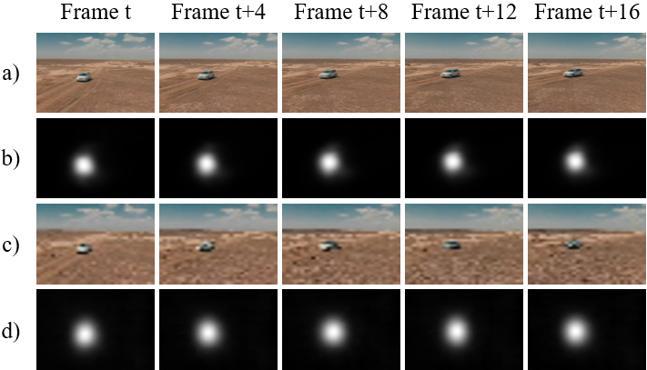
Figure 1: Comparison between the high-resolution and low-resolution videos. a) and b) are videos and their attention maps with high-resolution, while c) and d) are with low-resolution. Salient objects in low-resolution videos are missing much spatial information but still localizable.

However, due to the limited computational ability and memory space of such portable/wearable devices, there are two main issues in video attention prediction: 1) How to reduce the computational cost and memory space to enable the real-time applications on such devices? 2) How to extract powerful spatiotemporal features from videos to avoid remarkable loss of attention prediction accuracy? To address these two issues, it is necessary to explore a feasible solution that converts existing complex and sparse spatial and temporal attention models into a simple and compact spatiotemporal network.

Over the past years, deep learning has become the dominant approach in attention prediction due to its impressive capability of handling large-scale learning problems (?). Researchers tend to design more complex networks and collect more data for better performance. However, it has been proved that most of the complex networks are sparse and have a lot of redundancies. This fact facilitates the study of network compression, which aims to decrease computational and memory space cost. The video attention prediction can be greatly accelerated, but often at the expense of existing a prediction accuracy attenuation.

With the analyses in mind, we first reduce the resolution of the input image to $64\times 64$ which decreases the computational and memory space cost by about one order of magnitude. As demonstrated in Fig. 1, we observe that the salient objects in low-resolution videos are missing much spatial information but still localizable, which implies that it is still capable to recover the missing details. We then construct the network based on the depth-wise convolutions, which can further decrease the computational cost by about one order of magnitude and leads to an Ultrafast Video Attention Prediction Network (UVA-Net). However, UVA-Net will suffer from a dramatic performance decrease with a straight-forward training strategy. To this end, we propose a coupled knowledge distillation strategy, which can augment the model to discover and emphasize useful cues from the data and extract spatiotemporal features simultaneously.

The contributions of this work are summarized as follows: 1) We design an extremely lightweight spatiotemporal network with an ultrafast speed, which is 206 times faster than previous methods. 2) We propose a coupled knowledge distillation strategy to enable the network to effectively fuse the spatial and temporal features simultaneously and avoid remarkable loss of attention prediction accuracy. 3) Comprehensive experiments are conducted and illustrate that our model can achieve an ultrafast speed with a comparable attention prediction accuracy to the state-of-the-art models.

Related Work

In this section, we give a brief review of recent works from two perspectives: visual attention models as well as knowledge distillation and transfer.

Visual Attention Models

The heuristic models (?) can be roughly categorized into bottom-up approaches and top-down approaches. General models in the former category are stimulus-driven and compete to pop out visual signals. For example, Fang et al. (?) proposed a video attention model with a fusion strategy that according to the compactness and the temporal motion contrast. Later, Fang et al. (?) proposed another model that based on the uncertainty weighting. The models in the latter category are task-driven and usually integrating high-level factors.

In order to overcome the deficiency of the heuristic model fusion strategy, researchers have proposed plenty of non-deep learning models (?). Vig et al. (?) proposed a simple bottom-up attention model with supervised learning techniques fine-tune the free parameters for dynamic scenarios. Fang et al. (?) proposed an optimization framework with pairwise binary terms to pop out salient targets and suppressing distractors.

For further performance improvements, some deep learning models are proposed, which are emphasizing the importance of automatic hierarchical feature extraction and end-to-end learning (?). For example, Kümmerer et al. (?) directly used the features from VGG-19 network (?) for attention inference without additional fine-tuning. Pan et al. (?) proposed two networks for fixation prediction, with deep and shallow structures, respectively.

These modes can achieve impressive performance but usually have a high computational cost. How to obtain a speed-accuracy trade-off in attention prediction is still a key issue for scientific researchers.

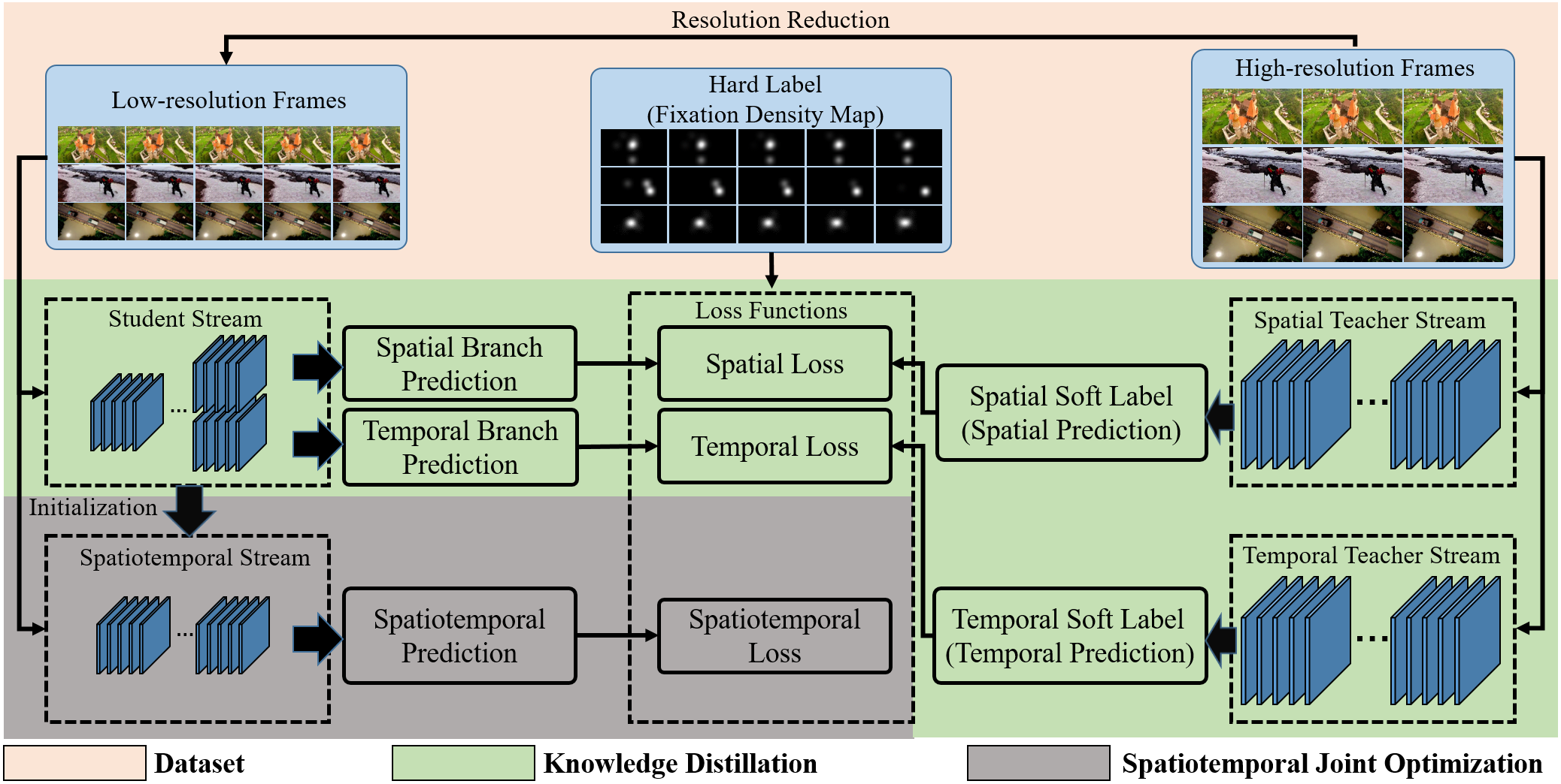
Figure 2: Overview. Our coupled knowledge distillation approach consists of four streams: a spatial teacher stream, a temporal teacher stream, a student stream and a spatiotemporal stream. It is trained in two steps: knowledge distillation and spatiotemporal joint optimization.

Knowledge Distillation and Transfer

Knowledge distillation is a class of techniques originally proposed by Hinton et al. (?), which aims at transferring knowledge in complex teacher model to simple student model and improving the performance of student model at test time. In (?), Hinton et al. adopt the soft labels generated by teacher model as the supervision signal in addition to the regular labeled training data during the training phase. Studies have shown that such extra supervision signal can be in various reasonable forms, such as classification probabilities (?), feature representation (?), or inter-layer flow (the inner product of feature maps) (?). It has observed a new wave of development exploiting knowledge transfer technologies to distill the knowledge in easy-to-train complex models into hard-to-train simple models.

There is no doubt that these knowledge distillation approaches are successful in high-resolution scenarios, but their effectiveness in low-resolution dynamic scenarios is questionable since they face the dual challenges of the limited network capacity and the loss of stimulus signal. With such questions, this paper demonstrates an ultrafast attention prediction network for videos.

Coupled Knowledge Distillation

In this section, we present a coupled knowledge distillation approach for video attention prediction.

Overview

We start with an overview of our coupled knowledge distillation approach before going into details below. We learn a strong yet efficient attention predictor by transferring the knowledge of a spatial teacher network and a temporal teacher network to a simple and compact one. The overview is as shown in Fig. 2.

The overall training process consists of two steps: 1) Knowledge distillation. Distilling the spatial and temporal knowledge inherited in the spatial teacher network and the temporal teacher network to a student network. 2) Spatiotemporal joint optimization. Transferring the knowledge learned by the student network to a spatiotemporal network and then fine-tune it.

Residual Block with Channel-wise Attention

Inspired by MobileNetV2 (?), we construct our networks with depth-wise convolutions with inverted residual structure. The basic convolutional blocks of MobileNet V2 are illustrated in Fig. 3 (a). Such blocks can greatly improve the compactness of the networks but hard to maintain the same accuracy. Aiming to meet the requirements of practical applications on resource-limited devices, we introduce channel-wise attention mechanism in MobileNet V2 blocks and propose a novel light-weight block, named as CA-Res block. Detailed architecture of CA-Res blocks are as shown in Fig. 3 (b).

Let $\textbf{R}_{in}$ and $\textbf{R}_{out}$ be the input and output intermediate representation, respectively. The $\textbf{R}_{out}$ can be formulated as

$$\textbf{R}_{out}=\textbf{R}_{in}+f^{inv}(\textbf{R}_{in})\odot f^{ca}(f^{inv}(\textbf{R}_{in})),$$ (1)

where $f^{inv}$ denotes the inverted residual structure of MobileNet V2 block, $f^{ca}$ refers to a channel-wise attention function, $\odot$ is element-wise multiplication. We denote global average pooling and global max pooling as $P^{avg}$ and $P^{max}$, respectively. In general, $P^{avg}$ performs well in preserving global characteristics, while $P^{max}$ has the potential to remain the texture features (?). It has been proved that exploiting both of them can greatly improve the representation power of networks than using each independently. Given an intermediate feature map F, we can model $f^{ca}$ via

$$f^{ca}(\textbf{F})=\sigma(f^{MLP}(P^{avg}(\textbf{F}))+f^{MLP}(P^{max}(\textbf{F}))),$$ (2)

where $f^{MLP}$ refers to a multi-layer perceptron (MLP) which functioned as a generator of attention vectors, and $\sigma$ is sigmoid function. Both of $P^{avg}$ and $P^{max}$ are used to squeeze the spatial dimension of F.

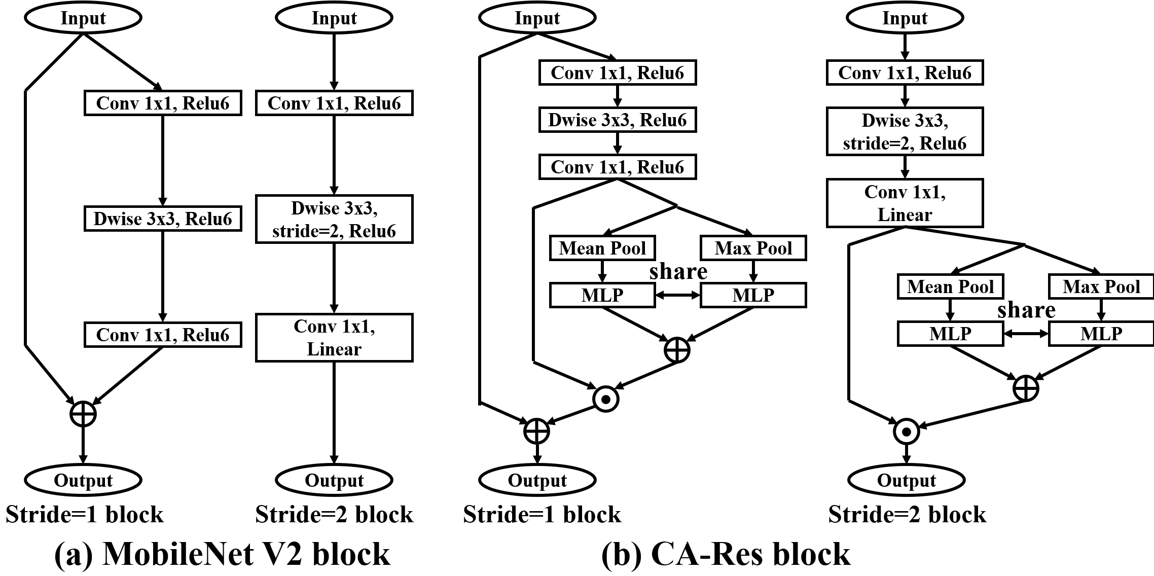
Figure 3: Detailed convolutional blocks. (a) MobileNet V2 block. (b) CA-Res block.

Knowledge Distillation

Given the CA-Res block, we now describe the details to construct our knowledge distillation network. Suppose that the dataset is given as $\mathcal{D}=\{I_{t},Y_{t}\}$, $t=1,2,3,\ldots,n$, where $I_{t}$ is an input image and $Y_{t}$ is a ground-truth map corresponding to $I_{t}$. Since this work aims to learn a spatiotemporal student model, the student architecture should be able to simulate the spatial/temporal features extracted by the teachers. Thus, our student network is a two-branch network that takes low-resolution successive frame pair $(I_{t},I_{t+1})$ as input, and outputs both spatially and temporally predicted attentions. Note that in teacher networks, the temporal information is often extracted with the assistance of optical flows, as it provides effective ways to smoothly accumulate features along time. However, optical flows are expensive to compute, and hard to be applied in a lightweight model.

To effectively mimic temporal features with low cost, we propose to adopt simple operations on immediate features, which have more representation power, to mimic the temporal dynamics. Specifically, given the frame pair $(I_{t},I_{t+1})$, the network first processes them through a low-level module $f^{s}$, which contains one stand convolutional layer and three CA-Res blocks in each branch, and shares the weights in the two paths. In this manner, the spatial intermediate representation $\mathcal{F}_{t}^{spa}$ and temporal intermediate representation $\mathcal{F}_{t}^{tem}$ can be computed via

$$\mathcal{F}_{t}^{spa} = f^{s}(I_{t}),$$ (3)

$$\mathcal{F}_{t}^{tem} = \mathrm{cat}\left(f^{s}(I_{t}),f^{s}(I_{t})-f^{s}(I_{t+1})\right),$$ (4)

where $\mathrm{cat}(\cdot)$ refers to a concatenating operation. We feed the $\mathcal{F}_{t}^{spa}$ into a spatial path, which consists of five blocks, to further extract high-level spatial intermediate representation $\mathcal{F}_{t}^{spa^{\prime}}$. Similarly, the $\mathcal{F}_{t}^{tem}$ is fed into a temporal path to extract high-level temporal intermediate representation $\mathcal{F}_{t}^{tem^{\prime}}$. Note that the spatial path and the temporal path share the same topology structure. Each path is followed with two deconvolutional layers to restore the $\mathcal{F}_{t}^{spa^{\prime}}$ and $\mathcal{F}_{t}^{tem^{\prime}}$ to fine feature map with the original resolution of input frames. The overall architecture of the student network is as shown in Fig. 4 (a).

We denote the spatial teacher, temporal teacher and student networks as $\mathbb{T}_{spa}$, $\mathbb{T}_{tem}$ and $\mathbb{S}$, respectively. Then, the $\mathbb{S}$ can be trained by optimizing spatial loss $\mathcal{L}_{spa}$ and temporal loss $\mathcal{L}_{tem}$

$$\begin{split}\mathcal{L}_{spa}=&(1-\mu)\cdot\mathcal{L}_{hard}(\mathbb{S}_{spa}(I_{t},I_{t+1}),Y_{t})\\ &+\mu\cdot\mathcal{L}_{soft}(\mathbb{S}_{spa}(I_{t},I_{t+1}),\mathbb{T}_{spa}(I_{t})),\end{split}$$ (5)

$$\begin{split}\mathcal{L}_{tem}=&(1-\mu)\cdot\mathcal{L}_{hard}(\mathbb{S}_{tem}(I_{t},I_{t+1}),Y_{t})\\ &+\mu\cdot\mathcal{L}_{soft}(\mathbb{S}_{tem}(I_{t},I_{t+1}),\mathbb{T}_{tem}(I_{t},I_{t+1})),\end{split}$$ (6)

where $\mathcal{L}_{hard}$ and $\mathcal{L}_{soft}$ denote the hard loss and soft loss, respectively. The hard loss is a $\ell_{2}$ loss associated with the predicted density map and the ground truth density map, while the soft loss is a $\ell_{2}$ loss associated with the predicted density map and the teacher prediction following the practice in knowledge distillation (?). The parameter $\mu$ balances $\mathcal{L}_{hard}$ and $\mathcal{L}_{soft}$ which we empirically set to $0.5$. $\mathbb{S}_{spa}$ and $\mathbb{S}_{tem}$ refer to the spatial and temporal branch of $\mathbb{S}$, respectively.

Spatiotemporal Joint Optimization

Although the student model $\mathbb{S}$ can distill spatial and temporal knowledge inherited in teacher networks to itself separately, it is still challenging to fuse the spatial and temporal features together to provide more powerful representations. To address this issue, we construct a spatiotemporal network, which is denoted as $\mathbb{S}_{sp}$. The first six blocks of $\mathbb{S}_{sp}$ share the same structure as with those of $\mathbb{S}$ to transferring the knowledge from the $\mathbb{S}$. In this manner, $\mathbb{S}_{sp}$ can generate both spatial intermediate representation $\mathcal{F}_{t}^{spa^{\prime\prime}}$ and temporal intermediate representation $\mathcal{F}_{t}^{tem^{\prime\prime}}$ like $\mathbb{S}$. Following the shared part, a fusion sub-net takes the concatenation of $\mathcal{F}_{t}^{spa^{\prime\prime}}$ and $\mathcal{F}_{t}^{tem^{\prime\prime}}$ as input, fuse them together, and infer the final spatiotemporal attention map $\mathcal{S}^{t}$

$$\mathcal{S}_{t}=f^{fuse}(\mathrm{cat}(\mathcal{F}_{t}^{spa^{\prime\prime}},\mathcal{F}_{t}^{tem^{\prime\prime}})),$$ (7)

where $f^{fuse}$ refers to the fusion sub-net. Note that the fusion sub-net has the same structure as the last five blocks except for its first block, which has doubled channels. The detail of $\mathbb{S}_{sp}$ is illustrated in Fig. 4 (b).

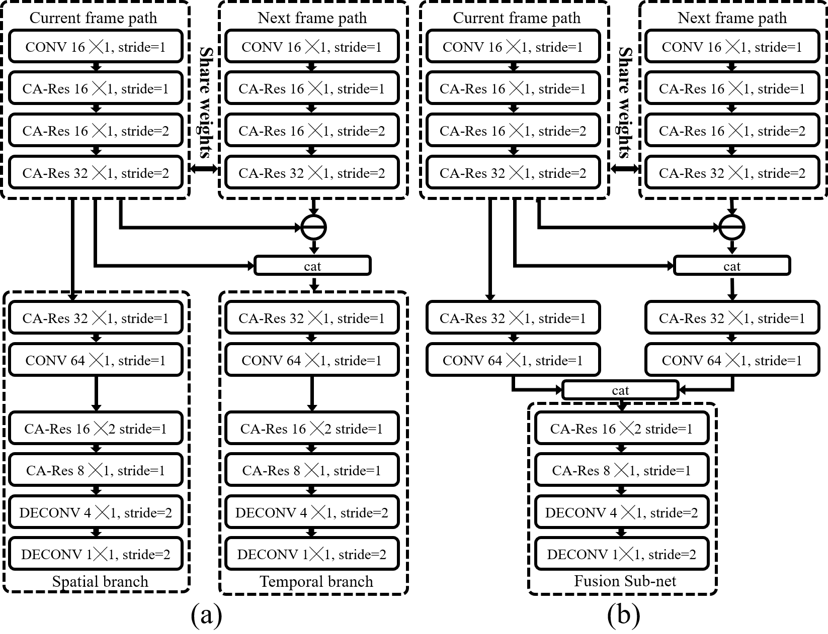
Figure 4: Network architecture. (a) Student network $\mathbb{S}$. (b) Spatiotemporal network $\mathbb{S}_{sp}$.

Different from $\mathbb{S}$, $\mathbb{S}_{sp}$ is trained by optimizing the spatiotemporal loss $\mathcal{L}_{sp}$, which is only related to the hard loss $\mathcal{L}_{hard}$

$$\mathcal{L}_{sp}=\mathcal{L}_{hard}(\mathbb{S}_{sp}(I_{t},I_{t+1}),Y_{t}).$$ (8)

Training Details

All networks proposed in this paper are implemented with Tensorflow (?) on an NVIDIA GPU 1080Ti and a six-core CPU Intel 3.4GHz. In the knowledge distillation step, $\mathbb{S}$ is trained from scratch with a learning rate of $5\times 10^{-4}$ and a batch size of 96. Adam (?) is employed to minimize the spatial loss $\mathcal{L}_{spa}$ and temporal loss $\mathcal{L}_{tmp}$. After training, the $\mathbb{S}$ performs well in extracting both spatial and temporal features from successive frame pair $(I_{t},I_{t+1})$. In the spatiotemporal joint optimization step, the knowledge inherited from $\mathbb{S}$ is transferred into $\mathbb{S}_{sp}$, by optimizing the $\mathcal{L}_{sp}$, $\mathbb{S}_{sp}$ can perform well in extracting the spatiotemporal features.

Experiments

We evaluate the proposed UVA-Net on a public dataset AVS1K (?), which is an aerial video dataset for attention prediction.

Table 1: Performance comparisons of 13 state-of-the-art models on AVS1K. The best and runner-up models of each column are marked with bold and underline, respectively. Except our model, the other deep models fine-tuned on AVS1K are marked with *.

Models		AUC	sAUC	NSS	SIM	CC	Input Resolution	Parameters (M)	Memory Footprint (MB)	Speed (fps)
										GPU (NVIDIA 1080Ti)	CPU (Intel 3.4GHz)
H	HFT	0.789	0.715	1.671	0.408	0.539	$128\times 128$	—	—	—	7.6
	SP	0.781	0.706	1.602	0.422	0.520	$\max\{h,w\}=320$	—	—	—	3.6
	PNSP	0.787	0.634	1.140	0.321	0.370	$400\times 400$	—	—	—	—
NL	SSD	0.737	0.692	1.564	0.404	0.503	$256\times 256$	—	—	—	2.9
	LDS	0.808	0.720	1.743	0.452	0.565	Original Size	—	—	—	4.6
DL	eDN	0.855	0.732	1.262	0.289	0.417	—	—	—	—	0.2
	iSEEL	0.801	0.767	1.974	0.458	0.636	$224\times 224$	—	—	—	—
	DVA∗	0.864	0.761	2.044	0.544	0.658	$224\times 224$	25.07	59.01	49	2.5
	SalNet∗	0.797	0.769	1.835	0.410	0.593	$224\times 224$	25.81	43.22	28	1.5
	TSNet∗	0.843	0.719	1.754	0.479	0.561	$224\times 224$	25.81	43.22	—	—
	STS∗	0.804	0.732	1.821	0.472	0.578	$320\times 320$	41.25	86.94	17	0.9
	UVA-DVA-32	0.850	0.740	1.905	0.522	0.615	$32\times 32$	0.16	0.68	10,106	404.3
	UVA-DVA-64	0.856	0.748	1.981	0.540	0.635	$64\times 64$	0.16	2.73	2,588	101.7

On the AVS1K, the UVA-Net is compared with 11 state-of-the-art models for video attention prediction, including:

1) Three heuristic models (group denoted as [H]): HFT (?), SP (?) and PNSP (?).

2) Two non-deep learning models (group denoted as [NL]): SSD (?) and LDS (?).

3) Six deep learning models (group denoted as [DL]): eDN (?), iSEEL (?), DVA (?), SalNet (?), TSNet (?) and STS (?).

With respect to the prior investigation of (?), we adopt five evaluation metrics in the comparisons, including the traditional Area Under the ROC Curve (AUC), the shuffled AUC (sAUC), the Normalized Scanpath Saliency (NSS), the Similarity Metric (SIM) (?), and the Correlation Coefficient (CC) (?).

Comparison with the State-of-the-art Models

The performance of 13 state-of-the-art models on AVS1K is presented in Tab. 1. For sake of simplicity, we take UVA-Net in the resolution of $32\times 32$ and $64\times 64$, fix the spatial and temporal teacher models as DVA and TSNet (?), respectively. Some representative results of those models are illustrated in Fig. 5.

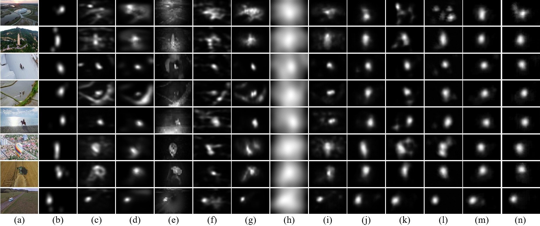
Figure 5: Representative frames of state-of-the-art models on AVS1K. (a) Video frame, (b) Ground truth, (c) HFT, (d) SP, (e) PNSP, (f) SSD, (g) LDS, (h) eDN, (i) iSEEL, (j) DVA, (k) SalNet, (l) STS, (m) UVA-DVA-32, (n) UVA-DVA-64.

From Tab. 1, we observe that both the UVA-DVA-32 and UVA-DVA-64 are comparable to the 11 state-of-the-art models. In terms of AUC, NSS, and SIM, the UVA-DVA-64 ranks the second place and its CC ranks the third place while its sAUC ranks the fourth place. Such impressive performance can be attributed to the coupled knowledge distillation approach, which distills the spatial and temporal knowledge from well-trained complex teacher networks to a simple and compact student network, and finally transfers it into a spatiotemporal network. The knowledge distillation step makes it capable for the spatiotemporal network to separately extracting spatial and temporal cues from successive frame pair, while the spatiotemporal joint optimization step gives the spatiotemporal network the ability to fuse such spatial and temporal cues together to provide more powerful representations. Specially, we find that the UVA-DVA-64 is superior to traditional single branch networks (such as SalNet, with a $8.0\%$ performance gain), two-branch networks for video (such as STS, with a $8.8\%$ performance gain), but slightly inferior to multi-branch structure networks (such as DVA, with a $3.1\%$ performance drop). In addition, our UVA-Net has extremely low parameters (only $0.16$ M) and low memory footprint (UVA-DVA-32 takes $0.68$ MB and UVA-DVA-64 takes $2.73$ MB), resulting in high computational efficiency. In summary, the UVA-DVA-64 achieves very fast speed ($404.3$ FPS) and comparable performance to the state-of-the-art models. The UVA-DVA-32 achieves ultrafast speed ($10,106$ FPS) but with slight performance degradation.

We conduct a scalability experiment on DHF1K and present its performance in Tab. 2 to verify the proposed model’s scalability to a ground-level dataset with normal viewpoints and target scales. Note that the DHF1K is the current largest ground-level video visual attention dataset and has made a significant leap in terms of scalability, diversity, and difficulty when compared with conventional ground-level datasets. On DHF1K, our model is compared with ten state-of-the-art models, including: PQFT (?), Seo et al. (?), Rudoy et al. (?), Hou et al. (?), Fang et al. (?), OBDL (?), AWS-D (?), OM-CNN (?), Two-stream (?). From this table, we find that our model is comparable with leading approaches, but runs two orders of magnitude faster.

Model	AUC	sAUC	NSS	SIM	CC	Speed (FPS)
PQFT	0.699	0.562	0.749	0.139	0.137	–
Seo et al.	0.635	0.499	0.334	0.142	0.070	–
Rudoy et al.	0.769	0.501	1.498	0.214	0.285	–
Hou et al.	0.726	0.545	0.847	0.167	0.150	–
Fang et al.	0.819	0.537	1.539	0.198	0.273	–
OBDL	0.638	0.500	0.495	0.171	0.117	–
AWS-D	0.703	0.513	0.940	0.157	0.174	–
OM-CNN	0.856	0.583	1.911	0.256	0.344	30
Two-stream	0.834	0.581	1.632	0.197	0.325	17
ACL	0.890	0.601	2.354	0.315	0.434	40
OUR*	0.833	0.582	1.536	0.241	0.307	2,588

• Models test on the validation set of DHF1K.

Table 2: Performance comparison of 11 state-of-the-art dynamic models on DHF1K. The best and runner-up of each column are marked with bold and underline, respectively.

Detailed Performance Analysis

Beyond performance comparisons, we also conduct several experiments on AVS1K to verify the effectiveness of the proposed UVA-Net.

Resolution reduction and supervision signal. We conduct an experiment to assess the resolution reduction and supervision signal. Without loss of generality, we fix the temporal teacher signal as TSNet, and provide three candidate spatial teacher signals, DVA, SalNet and SSNet (?) in resolution $256\times 256$, $128\times 128$, $96\times 96$, $64\times 64$ and $32\times 32$. The performance of UVA-Net with different settings are presented in Tab. 3.

Table 3: The performance comparisons of the UVA-Net with different settings on AVS1K dataset. T-S: spatial teacher model, Res: input resolution. The best model of each column in each spatial teacher signal are marked with bold.

T-S	Res	AUC	sAUC	NSS	SIM	CC
UVA-DVA	256	0.786	0.680	1.447	0.397	0.454
	128	0.810	0.698	1.566	0.438	0.498
	96	0.827	0.726	1.765	0.483	0.560
	64	0.856	0.748	1.981	0.540	0.635
	32	0.850	0.740	1.905	0.522	0.615
UVA-SalNet	256	0.775	0.676	1.423	0.394	0.451
	128	0.807	0.698	1.623	0.451	0.511
	96	0.843	0.717	1.746	0.484	0.551
	64	0.859	0.751	1.955	0.529	0.626
	32	0.852	0.739	1.892	0.519	0.611
UVA-SSNet	256	0.786	0.687	1.485	0.404	0.467
	128	0.807	0.703	1.641	0.455	0.517
	96	0.834	0.721	1.788	0.493	0.564
	64	0.852	0.744	1.971	0.535	0.627
	32	0.845	0.736	1.894	0.522	0.610

From this table, we find that models in low-resolution trends to have better performance. For example, with spatial supervision signal as DVA, the performance of UVA-Net in terms of all metrics in resolution $64\times 64$ ranks the first place. However, further resolution reduction will result in non-negligible performance degradation. We can infer that our UVA-Net can extract powerful spatiotemporal features from proper low-resolution videos, and it is still challenging for the UVA-Net in dealing with the details in high-resolution videos. In practical, compared with UVA-Net in $64\times 64$, the one with $256\times 256$ suffers from a $27.0\%$ performance drop.

Overall, the UVA-Net with DVA as teacher signal achieves the best performance, while SSNet and SalNet rank in the second and third places, respectively. For example, with resolution $64\times 64$, the UVA-Net supervised with DVA achieves NSS=$1.981$, while the SalNet and SSNet have only $1.955$ and $1.971$, respectively. This is consistent with the performance of teacher models in Tab. 1, which indicates the proposed approach can effectively transfer the knowledge inherited in teacher models.

Ablation study. We use the AVS1K dataset and adopt the UVA-Net with MobileNet V2 blocks trained from scratch as the baseline, denoted as MB+scratch. We empirically show the effectiveness of our design choice via six experiments. 1) MB+dis. The UVA-Net with MobileNet V2 blocks with coupled knowledge distillation. 2) MB+SE+dis. The UVA-Net with MobileNet V2 blocks and SE block with coupled knowledge distillation. 3) CA-Res+scratch. The UVA-Net with CA-Res blocks trained from scratch. 4) CA-Res+spa+scratch. The student network spatial branch with CA-Res blocks trained from scratch. 5) CA-Res+tmp+scratch. The student network temporal branch with CA-Res blocks trained from scratch. 6) CA-Res+dis. The UVA-Net with CA-Res blocks with coupled knowledge distillation. The performances of all these ablation models are described in Fig. 6.

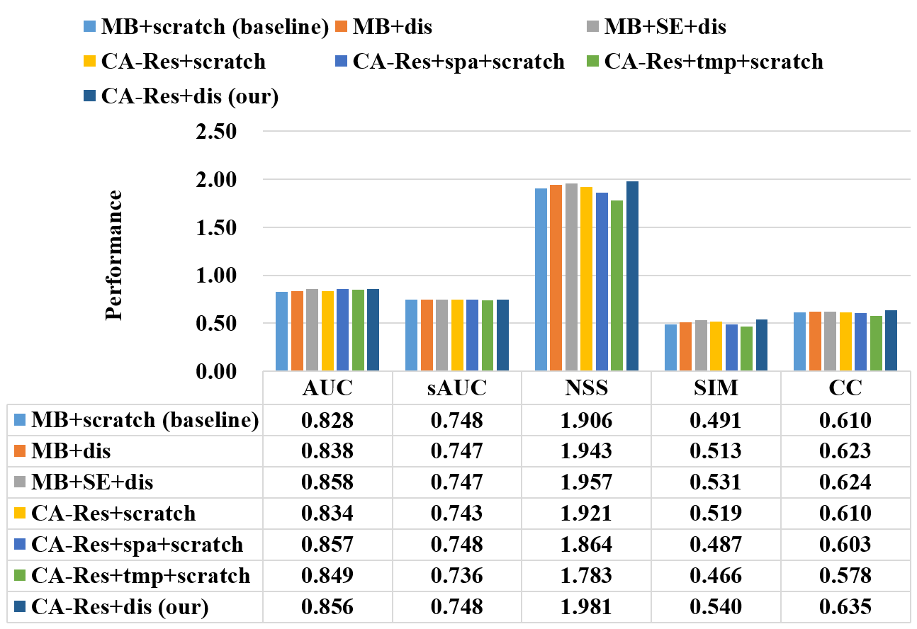
Figure 6: The performance comparisons of seven ablation models on AVS1K dataset.

From this figure, we find that CA-res+scratch achieves a performance gain to MB+scratch, i.e. NSS: $1.921\rightarrow 1.906$, and CA-res+dis is superior to MB+dis, i.e. NSS: $1.981\rightarrow 1.943$, which verify the effectiveness of the proposed channel-wise attention mechanism. Similarly, the effectiveness of our coupled knowledge distillation can be proved by the fact that MB+dis and CA-Res+dis are superior to MB+scratch and CA-Res+scratch, respectively. CA-Res+dis has a $2.0\%$ performance gain to MB+SE+dis, i.e. NSS: $1.981\rightarrow 1.943$, which infers the superior of our channel-wise attention mechanism to traditional SE block. The reason behind this may be that the SE block adopts global average pooling and ignore global max pooling, making it challenging in maintaining the texture characteristic of feature maps. Additionally, without spatiotemporal joint optimization, CA-Res+spa+dis and CA-Res+tem+dis have a non-negligible performance degradation to CA-Res+dis, i.e. NSS: $1.864\rightarrow 1.981$ and $1.783\rightarrow 1.981$, respectively. This verifies that exploiting both spatial and temporal cues can greatly improve the representation power of networks than using each independently.

Speed analysis. Our approach can greatly reduce the computational cost and memory space without remarkable loss of prediction accuracy. In particular, the DVA, SalNet, and STS contain $25.07$, $25.81$ and $41.25$ million parameters, while the proposed UVA-Net contains only $0.16$ million parameters. Namely, the UAV-Net achieves a substantial attenuation in the parameter amount. In addition, the memory footprints of UVA-Net in the different resolution are illustrated in Fig. 7.

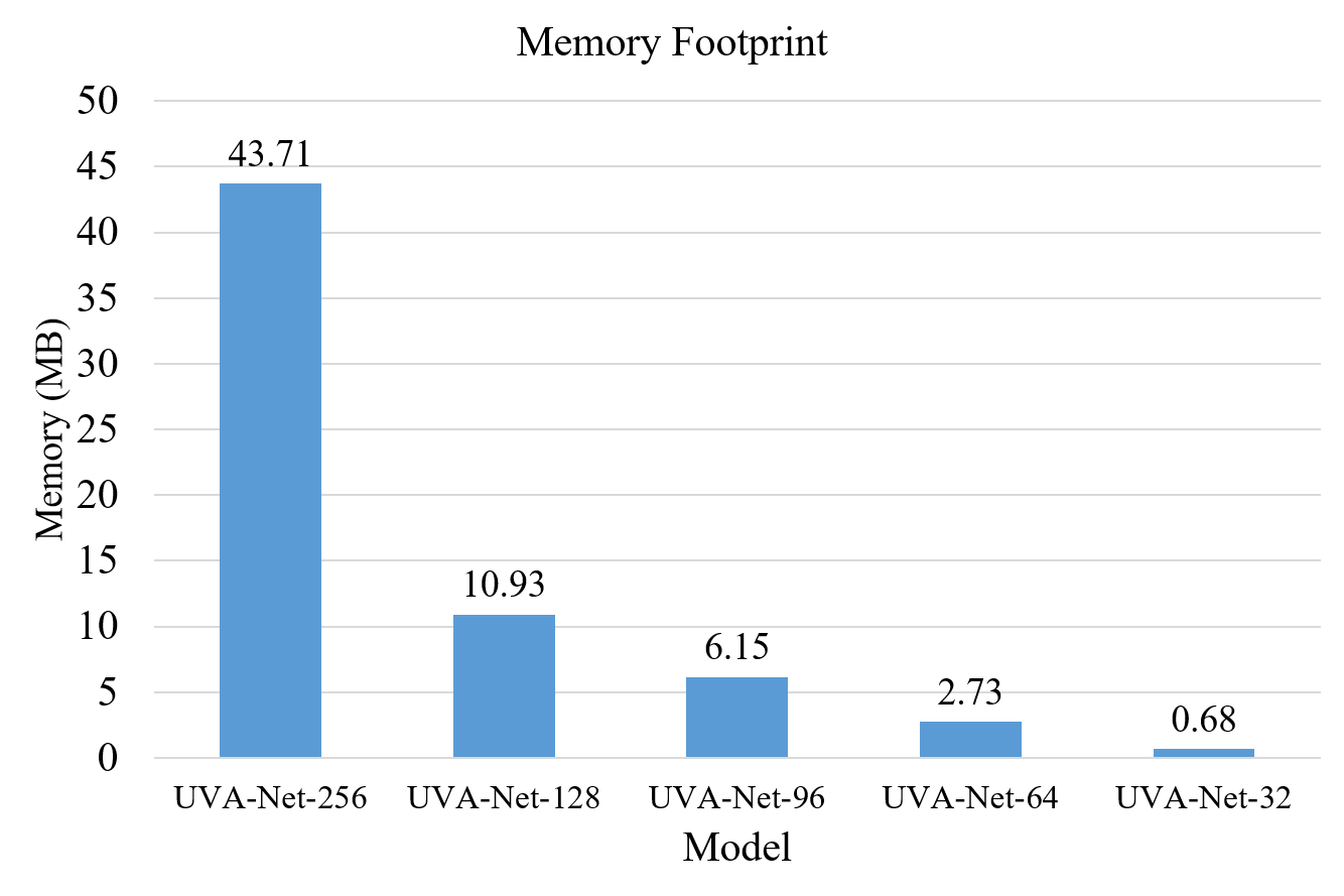
Figure 7: The inference memory footprint for various models. the memory footprint is proportional to the resolution of input.

We find that the memory footprint is proportional to the input resolution. For example, with a low resolution, such as $32\times 32$, the memory footprint of UVA-Net can be reduced to an extremely low value, $0.68$ MB. With such few parameters and low memory footprint, the process of attention inference can be greatly accelerated.

For comparison, we demonstrate the inference runtime of UVA-Net with different resolution on both high-end GPU (NVIDIA 1080Ti) and low-end CPU (Intel 3.4GHz) in Tab. 4.

Table 4: Inference time and speed on GPU and CPU.

Model	GPU (NVIDIA 1080Ti)	CPU (Intel 3.4GHz)
	time/#FPS	time/#FPS
UVA-Net-256	6.602 ms / 151	134.230 ms / 7.4
UVA-Net-128	1.586 ms / 631	40.928 ms / 24.4
UVA-Net-96	0.897 ms / 1,115	22.495 ms / 44.5
UVA-Net-64	0.386 ms / 2,588	9.830 ms / 101.7
UVA-Net-32	0.099 ms / 10,106	2.474 ms / 404.3

We observe that the inference runtime (with a NVIDIA 1080Ti) for attention prediction can be reduced to $6.602$ ms, $1.586$ ms, $0.897$ ms, $0.386$ ms and $0.099$ ms in resolution $256\times 256$, $128\times 128$, $96\times 96$, $64\times 64$ and $32\times 32$, respectively. Our model is a remarkable trade-off, which achieves ultrafast speed and impressive accuracy even with a CPU.

Conclusion

In this paper, we propose a simple yet powerful approach via coupled knowledge distillation for video attention prediction. In the knowledge distillation step, we distill the spatial and temporal knowledge inherited in the teacher networks to a student network. In the spatiotemporal joint optimization step, we transfer the knowledge learned by the student network to a spatiotemporal network and then fine-tune it. The proposed approach can greatly reduce the computational cost and memory space without remarkable loss of accuracy. The experimental results on a video dataset have validated the effectiveness of the proposed approach.

References

- [Abadi et al. 2016] Abadi, M.; Barham, P.; Chen, J.; Chen, Z.; Davis, A.; Dean, J.; Devin, M.; Ghemawat, S.; Irving, G.; Isard, M.; et al. 2016. Tensorflow: a system for large-scale machine learning. In OSDI, volume 16, 265–283.
- [Bak et al. 2017] Bak, C.; Kocak, A.; Erdem, E.; and Erdem, A. 2017. Spatio-temporal saliency networks for dynamic saliency prediction. IEEE TMM.
- [Borji 2012] Borji, A. 2012. Boosting bottom-up and top-down visual features for saliency estimation. In CVPR.
- [Bylinskii et al. 2018] Bylinskii, Z.; Judd, T.; Oliva, A.; Torralba, A.; and Durand, F. 2018. What do different evaluation metrics tell us about saliency models? IEEE TPAMI 41(3):740–757.
- [Deng et al. 2009] Deng, J.; Dong, W.; Socher, R.; Li, L.-J.; Li, K.; and Fei-Fei, L. 2009. Imagenet: A large-scale hierarchical image database. In CVPR.
- [Fang et al. 2014] Fang, Y.; Lin, W.; Chen, Z.; Tsai, C.-M.; and Lin, C.-W. 2014. A video saliency detection model in compressed domain. IEEE TCSVT 24(1):27–38.
- [Fang et al. 2017a] Fang, S.; Li, J.; Tian, Y.; Huang, T.; and Chen, X. 2017a. Learning discriminative subspaces on random contrasts for image saliency analysis. IEEE TNNLS 28(5):1095–1108.
- [Fang et al. 2017b] Fang, Y.; Zhang, C.; Li, J.; Lei, J.; Da Silva, M. P.; and Le Callet, P. 2017b. Visual attention modeling for stereoscopic video: a benchmark and computational model. IEEE TIP 26(10):4684–4696.
- [Fu et al. 2018] Fu, K.; Jia, L.; Hongze, S.; and Tian, Y. 2018. How drones look: Crowdsourced knowledge transfer for aerial video saliency prediction. arXiv preprint arXiv:1811.05625.
- [Guo and Zhang 2010] Guo, C., and Zhang, L. 2010. A novel multiresolution spatiotemporal saliency detection model and its applications in image and video compression. IEEE TIP 19(1):185–198.
- [Hinton, Vinyals, and Dean 2015] Hinton, G.; Vinyals, O.; and Dean, J. 2015. Distilling the knowledge in a neural network. stat 1050:9.
- [Hossein Khatoonabadi et al. 2015] Hossein Khatoonabadi, S.; Vasconcelos, N.; Bajic, I. V.; and Shan, Y. 2015. How many bits does it take for a stimulus to be salient? In CVPR, 5501–5510.
- [Hou and Zhang 2009] Hou, X., and Zhang, L. 2009. Dynamic visual attention: Searching for coding length increments. In NIPS.
- [Hou et al. 2013] Hou, W.; Gao, X.; Tao, D.; and Li, X. 2013. Visual saliency detection using information divergence. PR 46(10):2658–2669.
- [Jiang et al. 2018] Jiang, L.; Xu, M.; Liu, T.; Qiao, M.; and Wang, Z. 2018. Deepvs: A deep learning based video saliency prediction approach. In The European Conference on Computer Vision (ECCV).
- [Kingma and Ba 2014] Kingma, D., and Ba, J. 2014. Adam: A method for stochastic optimization. arXiv preprint arXiv:1412.6980.
- [Kümmerer, Wallis, and Bethge 2016] Kümmerer, M.; Wallis, T. S.; and Bethge, M. 2016. Deepgaze ii: Reading fixations from deep features trained on object recognition. arXiv preprint arXiv:1610.01563.
- [Leboran et al. 2016] Leboran, V.; Garcia-Diaz, A.; Fdez-Vidal, X. R.; and Pardo, X. M. 2016. Dynamic whitening saliency. IEEE TPAMI 39(5):893–907.
- [Li et al. 2010] Li, J.; Tian, Y.; Huang, T.; and Gao, W. 2010. Probabilistic multi-task learning for visual saliency estimation in video. IJCV 90(2):150–165.
- [Li et al. 2013] Li, J.; Levine, M. D.; An, X.; Xu, X.; and He, H. 2013. Visual saliency based on scale-space analysis in the frequency domain. IEEE TPAMI 35(4):996–1010.
- [Li et al. 2014] Li, N.; Ye, J.; Ji, Y.; Ling, H.; and Yu, J. 2014. Saliency detection on light field. In CVPR.
- [Li et al. 2015] Li, J.; Duan, L. Y.; Chen, X.; Huang, T.; and Tian, Y. 2015. Finding the secret of image saliency in the frequency domain. IEEE TPAMI 37(12):2428.
- [Li et al. 2016] Li, X.; Zhao, L.; Wei, L.; Yang, M.-H.; Wu, F.; Zhuang, Y.; Ling, H.; and Wang, J. 2016. Deepsaliency: Multi-task deep neural network model for salient object detection. IEEE TIP 25(8):3919–3930.
- [Li, Tian, and Huang 2014] Li, J.; Tian, Y.; and Huang, T. 2014. Visual saliency with statistical priors. IJCV 107(3):239–253.
- [Pan et al. 2016] Pan, J.; Sayrol, E.; Giroinieto, X.; Mcguinness, K.; and Oconnor, N. E. 2016. Shallow and deep convolutional networks for saliency prediction. In CVPR.
- [Romero et al. 2014] Romero, A.; Ballas, N.; Kahou, S. E.; Chassang, A.; Gatta, C.; and Bengio, Y. 2014. Fitnets: Hints for thin deep nets. arXiv preprint arXiv:1412.6550.
- [Rudoy et al. 2013] Rudoy, D.; Goldman, D. B.; Shechtman, E.; and Zelnik-Manor, L. 2013. Learning video saliency from human gaze using candidate selection. In CVPR, 1147–1154.
- [Sandler et al. 2018] Sandler, M.; Howard, A.; Zhu, M.; Zhmoginov, A.; and Chen, L.-C. 2018. Mobilenetv2: Inverted residuals and linear bottlenecks. In CVPR, 4510–4520.
- [Seo and Milanfar 2009] Seo, H. J., and Milanfar, P. 2009. Static and space-time visual saliency detection by self-resemblance. JOV 9(12):15–15.
- [Shu et al. 2015] Shu, T.; Xie, D.; Rothrock, B.; Todorovic, S.; and Chun Zhu, S. 2015. Joint inference of groups, events and human roles in aerial videos. In CVPR, 4576–4584.
- [Simonyan and Zisserman 2014] Simonyan, K., and Zisserman, A. 2014. Very deep convolutional networks for large-scale image recognition. arXiv preprint arXiv:1409.1556.
- [Tavakoli et al. 2017] Tavakoli, H. R.; Borji, A.; Laaksonen, J.; and Rahtu, E. 2017. Exploiting inter-image similarity and ensemble of extreme learners for fixation prediction using deep features. Neurocomputing 244:10–18.
- [Vig et al. 2012] Vig, E.; Dorr, M.; Martinetz, T.; and Barth, E. 2012. Intrinsic dimensionality predicts the saliency of natural dynamic scenes. IEEE TPAMI 34(6):1080–1091.
- [Vig, Dorr, and Cox 2014] Vig, E.; Dorr, M.; and Cox, D. 2014. Large-scale optimization of hierarchical features for saliency prediction in natural images. In CVPR.
- [Wang and Shen 2018] Wang, W., and Shen, J. 2018. Deep visual attention prediction. IEEE TIP 27(5):2368–2378.
- [Woo et al. 2018] Woo, S.; Park, J.; Lee, J.-Y.; and So Kweon, I. 2018. Cbam: Convolutional block attention module. In ECCV, 3–19.
- [Yim et al. 2017] Yim, J.; Joo, D.; Bae, J.; and Kim, J. 2017. A gift from knowledge distillation: Fast optimization, network minimization and transfer learning. In CVPR, volume 2.
- [Zhang et al. 2010] Zhang, J.; Wu, Y.; Liu, W.; and Chen, X. 2010. Novel approach to position and orientation estimation in vision-based uav navigation. IEEE TAES 46(2):687–700.