An Systematic Analysis of Stellar Population in the Host Galaxies of SDSS Type I QSOs

Abstract

We investigate the relationship between host galaxies’ stellar content and active galactic nuclei (AGN) for optically selected QSOs with z$<$0.5. There are total 82 QSOs we select from Sloan Digital Sky Survey (SDSS) . These 82 QSOs both have Wide-field Infrared Survey Explorer (WISE) data and measurable stellar content. With the help of the stellar population synthesis code STARLIGHT, we determine the luminosity fraction of AGN ,stellar population ages and star-formation history (SFH) of host galaxies. We find out there is a correlation between the star formation history and AGN property which suggests a possible delay from star formation to AGN. This probably indicates that the AGN activity correlate with the star formation activity which consistent with a co-evolution scheme for black hole and host galaxies.

1 Introduction

The connection between active galactic nuclei (AGN) and starburst (SB) activity in galaxies have been proposed for a long time, going back to the first discovery of Ultraluminous Infrared Galaxies (ULIRGs) . Many effort has been made to drive out what is the dominant energy output mechanism (Rieke & Low, 1972; Rieke & Lebofsky, 1979; Sanders et al., 1988; Zou et al., 1991). More and more works have provided evidence that ULIRGs are powerd by a mixture of SB and AGN (Toomre & Toomre, 1972; Toomre, 1977; Sanders et al., 1988; Barnes & Hernquist, 1991, 1992, 1996; Zou et al., 1991; Wu et al., 1998a, b; Zheng et al., 1999; Cui et al., 2001; Xia et al., 2002; Springel et al., 2005; Cao et al., 2006). Sanders et al. (1988) has proposed a evolution scenario where two gas-rich spirals merge first and then drive gas into the merger center, triggering nuclear SB before the ignition of a dust-enshrouded AGN. When the dust has been consumed or swept away by the strong outflow from AGN and supernovae, an optical quasar would appear. Meanwhile these strong outflow also quench the star formation and the growth of black hole. Eventually, this evolution path provides a plausible explanation for the tight correlation between black hole mass and bugle of their host galaxies (Magorrian et al., 1998; Gebhardt et al., 2000; Ferrarese & Merritt, 2000; Tremaine et al., 2002; Kormendy & Gebhardt, 2001; Merritt & Ferrarese, 2001). Many studies also show that the black hole (BH) growth and star formation history has similar evolution (Hopkins, 2004; Silverman et al., 2008; Aird et al., 2010). By the way, the works of Taniguchi (1999) and Barth et al. (2008) shows that minor merges are also able to trigger the nuclear activity. Recent studies (Davies et al., 2007; Hopkins, 2012; Canalizo & Stockton, 2013; Zhang-hu & Qiu-sheng, 2016; Blank & Duschl, 2016) also suggested that AGN and SB activity may not contemporaneous and there is a time gap between AGN activity and star burst, but it is still a controversial argument (Magorrian et al., 1998; Gebhardt et al., 2000; Di Matteo et al., 2005).

In a word, at least one of the consequence of major-merger evolutionary scenarios is the existence of object which have a phase with both luminous quasar activity and post-starburst (or on-going star formation) signatures. So it is important to investigate the stellar population in QSOs host galaxies. In the work of McLure et al. (1999), they presented the HST imaging study and found that the R-K colors of host galaxies is consistent with mature stellar population. Nolan et al. (2001) fitted deep off-nuclear optical spectra of QSOs and found that the host galaxies are dominated by old stars. On the other hand, the close relationship between gas-rich mergers and nuclear activity was supported by several studies, which show a existence of recent star bursts in the host galaxies of QSOs. Kauffmann et al. (2003) examined the properties of the host galaxies of narrow-line AGN and found that the host of high-luminosity AGN has much younger mean stellar age.

Rembold et al. (2017) presented the characterization of the first 62 MaNGA (Mapping Nearby Galaxies at the Apache Point Observatory) AGN hosts and found that for more luminous AGNs the contribution of younger stellar populations to the optical emission is larger than for low-luminosity ones. Sánchez et al. (2018) presented the properties of a sample of 98 AGN host galaxies (both type-II and type-I) and found that AGN hosts are in the transition stage between star-forming and non-star-forming galaxies. There are also many other works that found similar results (Canalizo & Stockton, 2001; Sánchez et al., 2004; Letawe et al., 2007; Jahnke et al., 2007; Wold et al., 2010).

However, the overwhelming luminosity of QSOs compared with the host galaxies is a difficult challenge because both the AGN’s continuum and broad line will serious weaken the stellar features. Many remarkable works have been made over the past few years (as mentioned above) for their own motivations. For example, many works limited their sample to obscured AGNs whose centers are obscured by large amounts of dust so that their host galaxies can be studied (Davies et al., 2007; Kauffmann et al., 2003; Tadhunter et al., 2005; York et al., 2000; Heckman et al., 2004). Some works present an off-axis observation to avoid QSOs contamination (Nolan et al., 2001; Canalizo & Stockton, 2013), but this method may miss the young stellar population that may be present in the center of the galaxies. By performing the deconvolution method on 2-D spectra (Magain et al., 1998), Letawe et al. (2007) separated the individual spectra of QSOs and their host galaxies. There are also many works about post star-burst QSOs (PSQs) (Canalizo et al., 2000; Cales et al., 2013; Wei et al., 2013), which have prominent Balmer absorptions from A-type stars, but one must note that because of the definition, these objects were selected to have moderate-age stellar population by design.

Because the relationship between QSOs and their host galaxies has an important consequences in our understanding of galaxies evolution, it is necessary to investigate the QSOs’ host stellar population. In this paper we perform an extensive and statistical analyses for source selected from Sloan Digital Sky Survey (SDSS) (York et al., 2000; Stoughton et al., 2002). We effectively select the objects with distinct stellar feature for the first time and study their stellar population, mid-IR color as well as AGN properties. We describe the sample selection and data reductions in Section 2. The method for decomposing AGNs and stellar population along with star formation history (SFH) in Section 3. The outputted results and the properties of these QSOs as well as stellar population of host galaxies are given in Section 4. A discussion in Section 5 and the summary of our result is given in Section 6. We adopt the cosmology $H_{0}=70kms^{-1}Mpc^{-1}$ and a flat universe where $\Omega_{M}=0.3$ and $\Omega_{\Lambda}=0.7$.

2 Sample Selection

The data we use are selected from the quasar catalog (Schneider et al., 2010) of Sloan Digital Sky Survey data release 7 (SDSS DR7). The SDSS used a dedicated 2.5m wild-field telescope (Gunn et al., 2006) to image the sky in five broad bands ($u,g,r,i,z$). The QSOs candidates were selected based on their colors (Richards et al., 2002) and then observed with fiber-fed double spectrographs with 3^′′ diameter fiber which result in getting more emission from host galaxies. . SDSS DR7 quasars catalog contains 105,785 QSOs. In this study, we used the reduced one-dimensional spectral data derived from SDSS DR12 pipeline-processed. The spectra have a wavelength coverage of 3800-9200$\AA$ at a spectral resolution R $\sim$ 1500-2500.

In order to have a better understanding on the infrared properties of our sources, we built a parent sample by matching SDSS objects with the Wide-field Infrared Survey Explorer (WISE) in 3^′′ radius. The survey of WISE covers $95\%$ of sky at 3.4 (W1), 4.6 (W2), 12 (W3), 22 (W4) $\mu m$ with an angular resolution of 6.1^′′, 6.4^′′, 6.5^′′ and 12.0^′′ in four bands, achieving, $5\sigma$ point source sensitivities better than 0.08, 0.11, 1, and 6 $mJy$, respectively. We also set the upper limit of the redshift range to $z<0.5$ for two reason: 1) to reject the higher redshift QSOs because they have more luminous AGN which will dilutes the stellar feature; 2) this redshift range allows the spectral to covering the absorption line needed for $STARLIGHT$ analysis. In summary, the parent sample was built as follows:

1. $z<0.5$,

2. $(S/N)_{WISE}$ of W1, W2, W3 and W4 $>3$,

3. $(S/N)_{SDSS}\geq 15$,

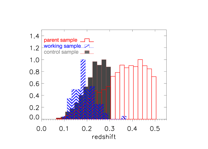
Figure 1: Redshift distribution for source in the parent sample (red blank), the working sample (blue diagonal) and the control sample (gray filled). The peaks are normalized to one.

where the $(S/N)_{WISE}$ represents the signal-to-noise ratio of photometry in WISE bands and the $(S/N)_{SDSS}$ is the signal-to-noise ratio of the SDSS spectra. There are total 8490 objects in our parent sample and Figure 1 shows the redshift distribution (red solid line).

Then, we selected the working sample from the parent sample by adding this criterion:

$(S/N)_{stellar}\geq 15$,

where the $(S/N)_{stellar}$ is the S/N of stellar composition which were calculated by using synthesis code $STARLIGHT$ and the detail of it will be given in $section3.1.1$.

Since the type I QSOs provide great observational challenge owing to their overwhelming brightness of the AGN with respect to the host galaxy, we use above criterion to ensure that all object in the sample have obvious stellar content. At last, there are total 82 objects in the working sample. Table LABEL:table:observation shows some observational properties of the sources in the working sample. Figure 1 shows the redshift distribution of these source (blue diagonal). The decrease of number of the sources in the working sample in high redshift (only one higher than 0.3) may result from the selection effect that brighter AGNs are more easy to be observed in high redshift and the host galaxy is overwhelmed by these brighter AGN.

We also extracted from the parent sample a control sample of QSOs which don’t have obvious stellar content. The control sample meeting this criteria:

$(S/N)_{stellar}<15$.

We also limit the redshift of our control sample to $z<0.3$. The final control sample is composed of 2183 objects. Figure 1 shows the redshift distribution of the parent sample (red solid line), the working sample (blued diagonal) and the control smaple (gray filled), respectively. We normalize them to 1.0 as peak of each.

We have to emphasize that the selection method used in this work is different from those preceding ones: 1) This work focuses on the stellar content of type I QSOs which are brighter than $M_{i}=-22\ mag$. In contrast, many works foucused on low-luminosity type II AGNs (Kauffmann et al., 2003; Yesuf et al., 2014; Davies et al., 2007; Kauffmann et al., 2003; Tadhunter et al., 2005; York et al., 2000; Heckman et al., 2004). 2) We attempt to study the stellar population of QSOs host which contain the central region of galaxies while some other’s work avoid QSOs contamination by off-axis observation (the spectra are obtained with the slit of the spectrograph located a few arcseconds away from the quasar) (Nolan et al., 2001; Canalizo & Stockton, 2013). 3) We don’t limit our working sample exclusive to QSOs host with moderate-age stellar population (PSQs), as done by some authors (Canalizo et al., 2000; Cales et al., 2013; Wei et al., 2013).

3 Spectral analysis

3.1 Spetral Synthesis with Starlight

We used the spectral analysis code $STARLIGHT$ (Cid Fernandes et al., 2005) to study the stellar population of host galaxies in our working sample. This code searches for the linear combination of $N_{*}$ Simple Stellar Populations (SSP) from evolutionary synthesis models for a best matches of observed spectrum $O_{\lambda}$. The models $M_{\lambda}$ is given by:

$M_{\lambda}=M_{\lambda_{0}}(\sum_{j=1}^{N_{*}}x_{j}b_{j,\lambda}r_{\lambda})\otimes G(v_{\star},\sigma_{\star})$,

where $b_{j,\lambda}$ is the normalized flux of the $j$th SSP at $\lambda_{0}$, $r_{\lambda}\equiv 10^{-0.4(A_{\lambda}-A_{\lambda_{0}})}$ is the reddening term, $M_{\lambda_{0}}$ is the synthetic flux at the normalization wavelength, $x_{j}$ is the population vector and $\otimes$ denotes the convolution operator and G is a Gaussian filter centered at velocity $v_{\star}$ and with dispersion $\sigma_{\star}$. This method carries out the fitting with a mixture of simulated annealing plus Metropolis scheme and Markov Chain Monte Carlo techniques to yield the minimum $\chi^{2}$ value ($\chi^{2}=\sum_{\lambda}[(O_{\lambda}-M_{\lambda})\omega_{\lambda}]$, where $M_{\lambda}$ is the model spectrum and ${\omega_{\lambda}}^{-1}$ is the error in $O_{\lambda}$ at each wavelength bin). The $\chi^{2}/N_{\lambda}$ which we used in $Section3.1.2.$ is the fit $\chi^{2}$ divided by the number of $\lambda$’s used in the fit.

3.1.1 Preliminary Fitting

Firstly, we used $STARLIGHT$ to fit the integrated spectra for all sources in the parent sample to get the luminosity ratio between the stellar population and AGN. The $STARLIGHT$ is a smarter and fast way of fitting a spectrum and it allows us to contain a power-law. We use SSPs models from Bruzual & Charlot (2003, BC03) (with $N_{\star}=150$ spectra of 6 metallicaties range from 0.0001 to 0.05 and 25 different ages range from 1Myr to 18Gyr). The reason why we chose BC03 is that it has a wide range of metallicities and it is also widely used in the literature which allowed us to have a comparison between our result and previous works. What’s more, the BC03 is the base model for $STARLIGHT$, so it is convenient to use them together. Though the BC03 has a new version (CB07, Charlot & Bruzual (2007)) which includes the new stellar evolution prescription for the TP-AGB evolution., the work (Zibetti et al., 2013) shown that the BC03 model is still the most successful in reproducing the stellar population of host galaxies. We also add a power-law spectrum $F_{\lambda}\propto\lambda^{\alpha_{\lambda}}$ which represent the contribution of AGN featureless continuum for preliminary fitting. The power-law spectra index $\alpha$ is -2 which is a traditional value of type 1 QSOs (Letawe et al., 2007; Vanden Berk et al., 2001; Shen et al., 2011). The Calzetti law (Calzetti et al., 2000) were used for the reddening during the fitting. We corrected for Galactic extinction using the Schlegel et al. (1998) maps and extinction curves from Fitzpatrick (1999). The input spectra to $STARLIGHT$ contain 4 columns: the wavelength ($\lambda$), the flux ($O_{\lambda}$), the error of flux ($e_{\lambda}$) and the $flag_{\lambda}$ which signals if that pixcel is good or bad. All these message of input spectrum are get from SDSS data release 12.

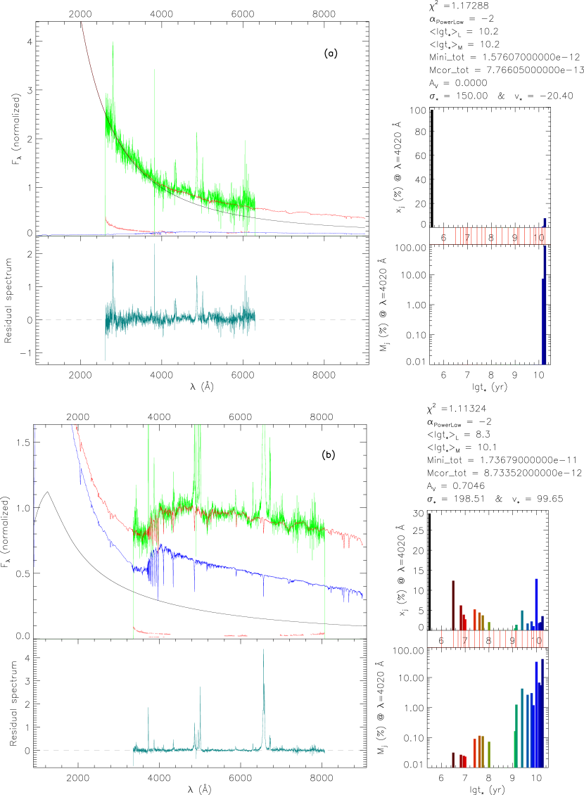
Figure 2: Spectral synthesis of SDSS DR7 QSOs. Panel (a) illustrated QSOs dominated by AGN (SDSS J000011.41+145545.6)—Top left : the observed spectrum $O_{\lambda}$(green), the model spectrum $N_{\lambda}$(red), the host galaxy starlight (blue) ,the power-law (black) and the error spectrum (pink) with the gaps meaning the masked regions and the five times weighted absorption lines. Bottom left: the residual spectrum (dark green). Right: light (top) and mass (bottom) weighted stellar population fraction $x_{j}$ and $\mu_{j}$,respectively. The inserted panel on the right marks the ages of the stellar population templates; Panel (b) illustrated QSOs dominated by stellar population (SDSS J131750.32+601040.8) which has obvious stellar feature such as strong Balmer absorption lines. The meaning of symbols are same as those Figure (a).

Figure 2 shows the result of $STARLIGHT$ fitting: the panel (a) is about a normal QSOs from control sample compared with panel (b) representing the objects of the working sample. Figure 2 (a) shows that most QSOs are dominated by AGN (the luminosity fraction of AGN is almost $100\%$) which can described by a power-law and shows little stellar feature in its spectrum.

In order to gain a sample of QSOs with significant stellar component, we calculate the S/N of host galaxy by

${(S/N)}_{stellar}={(S/N)}_{SDSS}\cdot\sqrt{1-\eta}$,

where $\eta$ is the luminosity ratio between the AGN and (AGN+host) getting from $STARLIGHT$ fitting; The ${(S/N)}_{stellar}$ is the signal-to-noise ratio of host galaxy. We require the ${(S/N)}_{stellar}$ greater than 15 and the subsample of our sources is total 82 objects. Figure 2 (b) show an example in the working sample which are dominated by stellar population with significant stellar feature in its spectrum such as $Ca_{II}$K $\lambda$3933, $Ca_{II}$H $\lambda$3968 and Balmer absorption lines.

3.1.2 Formal Fitting and Stellar Populations

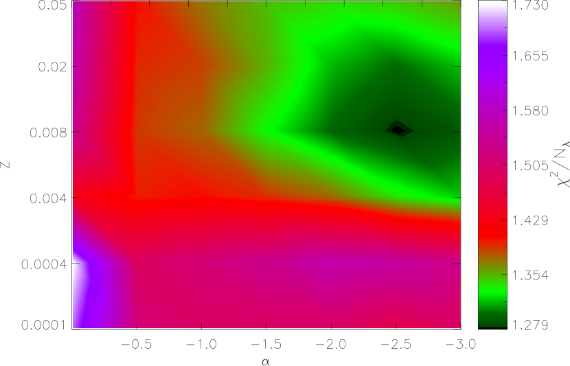
Figure 3: The test fitting of power-law index and metallicity. This figure shows the averaged $\chi^{2}/N_{\lambda}$ changed with metallicities (Z) and power-law indices ($\alpha$). The color bar is $\chi^{2}/N_{\lambda}$.

To make the result more reliable, we get the best-fit metallicity and power-law index by using method proposed by Meng et al. (2010). We adopted a wide range of AGN power-law slop $\alpha_{\lambda}$ over the optical and UV range from -3.0 to 0 (no power-law fitting with $\alpha_{\lambda}$=0) at intervals of 0.5 to search for the best power-law index. To search for the best-fit metallicity, we carry out a metallicity test with six metallicities ($Z=0.0001,0.0004,0.004,0.008,0.02,0.05$) of the BC03 model for each power-law index. Figure 3 shows the test fitting results for one example object with different power-law index $\alpha_{\lambda}$ and six metallicities. We evaluate the fitting quality by the minimum $\chi^{2}/N_{\lambda}$which is suggested by Cid Fernandes et al. (2005). We averaged it over 100 times fitting with different seed (the random number that need to be appointed during the $STARLIGHT$ fitting).

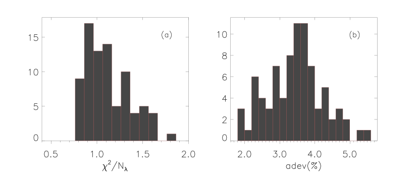
Figure 5: The distribution of $\chi^{2}/N_{\lambda}$ (panel a) and $adev$ (panel b) , the percentage mean $|O_{\lambda}-M_{\lambda}|/O_{\lambda}$ deviation over all fitted pixels, for 82 sources of the working sample.

As for the given metallicity and power law index, there are total 100 fitting results. Though difference result from random seeds will not change the overall population distribution, a $\sim 10\%$ variation may added to the individual component $x_{j}$ (Meng et al., 2010). In order to get a statistically reliable result, we selected the fitting result of minimal $\chi^{2}/N_{\lambda}$ value (if we have) or mean value over 100 fitting as the best fitting. Figure 4 shows the distribution of luminosity fraction of AGN ($frac_{AGN}$) and $\chi^{2}/N_{\lambda}$ for two objects in our working sample: we adopt the minimal and mean value in left and right panel, respectively. Besides the $\chi^{2}/N_{\lambda}$ value, we also use the adev vale as an indicator of the quality of fit. The adev gives the percentage mean $|O_{\lambda}-M_{\lambda}|/O_{\lambda}$ deviation over all fitted pixels. The Figure 5 shows the distribution of $\chi^{2}/N_{\lambda}$ value (Panel.a) and adev (Panel.b). Most of sources has a reliable fitting result with $\chi^{2}/N_{\lambda}$ $\sim$ 1. There are  22% (18/82) sources have $\chi^{2}/N_{\lambda}\geq 1.3$ . We find that the main reason accounting for this high $\chi^{2}/N_{\lambda}$ value is related to the fact that some high $frac_{AGN}$ objects are more difficult to fit because of lower stellar content. We have compare the main result getting from the data that contained these 18 objects and the data that do not contain these objects and found that there is no bias between them. So we keep these 18 objects in our work. The adev valus distribution is shown in Figure 5 (b) and presents values adev $\lesssim 6$ per cent for all objects, indicating that the model reproduces very well the observed underlying spectra.

3.2 Classification with SFH

We calculate the luminosity of the stellar component from UV to optical during the past $\sim$ 1Gyr by reconstructing the UV-to-Optical spectrum. The detailed descriptions of calculation can be found in Meng et al. (2010) and we briefly described the method here.

Because the 3^′′ diameter fiber does not cover the whole galaxy, a aperture corrections (Meng et al., 2010) are necessary. It is known that the luminosity of the galaxy is dominated by young stellar populations and the AGN, which can both be better traced by the u band, so we adopt the aperture correction for stellar component at the $u$ band derived from

$A=\frac{L_{\star Petro}}{L\star fiber}=\frac{10^{-0.4(m_{petro}-m_{AGN})-1}}{10^{-0.4(m_{fiber}-m_{AGN})-1}}$.

We rebuild the rest-frame model spectrum $F_{i}(\lambda,t)$ of stellar with whole UV-to-Optical wavelengths coverage ($912\sim 9000\AA$) corrected for extinction by

$F_{i}(\lambda,t)=Mcor\_tot\sum_{j=1}^{N}\frac{\mu_{j}}{f_{\star,j,t_{0}}}f_{\star,j,t}B_{\lambda,j,t}$,

where $F_{i}(\lambda,t)$ is the stellar spectrum (corrected for extinction) at a given time $t$. $t$ can be the time in the past or at the present (equal $t_{0}$). $Mcor\_tot$ is present stellar mass obtained from the spectral synthesis after aperture correction, $\mu_{j}$ is mass-weighted fraction, $B_{\lambda,j,t}$ are BC03 SSP templates without normalization, $f_{\star,j,t_{0}}$ is the present ($t_{0}$) fraction of remaining stellar mass to the initial mass of population $j$, $f_{\star,j,t}$ is such fraction at a given time $t$. We estimate the UV-to-Optical luminosity of the past 25, 100, 290, 500 and 900 Myr separately.

we calculate the UV-to-Optical luminosity history of the host galaxies by

$L_{UV\_Optical,t}=\int_{912}^{9000}[F_{i}(\lambda,t)]d\lambda$ .

To test the feasibility of our method, we also reconstructed the spectrum in present time ($t_{0}$) by adding the dust extinction and double-index power. The formula is

$F_{0}(\lambda,t_{0})=[L_{UV\_Optical,0}+F_{p}(\lambda)]\times 10^{-0.4(A_{\lambda}-A_{V})}$,

where $F_{p}(\lambda)$ is a double power-law spectrum of AGN. The spectral indexes we used here are given by $\alpha=-1$ for $\lambda<1250\AA$ (Hatziminaoglou et al., 2008) and $\alpha$ given by starlight for $\lambda>1250\AA$. The $A_{V}$ is obtained from the spectral synthesis. Figure LABEL:fig:history shows the reconstructed model spectrum (red solid line) superimposed by the observed one (green solid line). This model spectrum is used as $F_{0}(\lambda,t_{0})$.

At last, we give a simple classification of our working sample based on the SFH ($L_{UV\_Optical,t}$) of the host galaxy. In summary, there are two main features of these SFH: one is a dramatically enhanced star formation about 900 Myr ago, and moderate one recently (with in 500 Myr). Since their prototypes are unknown, we focus on these two features and attempt to classify our source according to their SFH in our work. At last, we classify our working sample into 4 types:

(1)$typeO$ : Don’t have obvious star formation activity in the past 900 Myr. The star formation activity in this objects could took place 1 Gyr ago. There are total 16 sources in this type.

(2)$typeA$ : Only have moderate star formation activity within 500Myr. There are total 20 sources in this type;

(3)$typeB$ : Only have dramatically enhanced star formation activity about 900 Myr ago. There are total 11 sources in this type;

(4)$typeAB$ : Have both two main feature of SFH ( dramatically enhanced one and moderate one). There are total 35 sources in this type.

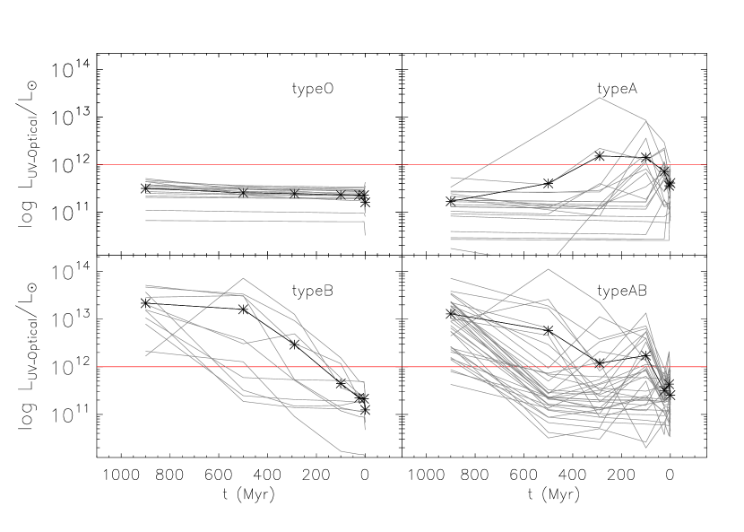
Figure 7: The four panels display the averaged $L_{UV\_Optical}$ (912-9000 $\AA$) of source of the working sample of four different types: $typeO$, $typeA$, $typeB$ and $typeAB$. The gray lines represent the individual objects for corresponding classes.

Figure 7 shows the mean star formation histories of these four different type (dark line) which is added with individual objects ( gray lines ) for corresponding classes.

4 Result & Analysis

4.1 Composite Spectra

In order to characterize the spectrum-to-spectrum difference for these four SFH types, we make a combination for each type by normalizing each individual spectrum at 5100$\AA$ and then computing the average value of $F_{\lambda}$ in bins of $\lambda$.

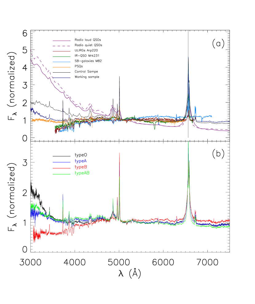
Figure 8: The panel (a) shows the composite spectra of the radio loud QSOs (solid purple line), radio quiet QSOs (dash purple line), PSQs (orange line), IR QSOs (dark green line), ULIRGs (dark red line), starburst galaxy (cyan blue line) and the control sample (black line); The panel (b) shows the composite spectra of: $typeO$ (black), $typeA$ (blue), $typeB$ (red) and $typeAB$ (green).

Figure 8 shows the composites spectral of sources sample in the working . For more explicit, we divide the spectrum into two panels. In the panel (a), we compare composite spectrum of the souses in the working sample (blue solid line) with those of others. For example, we plot the QSOs spectra from Shang et al. (2011), which presented the SEDs of 85 optically bright, non-blazar QSOs (27 radio-quiet and 58 radio-loud) over the wavelength from radio to X-ray. The purple solid line represents the radio-loud QSOs and the purple dashed line represents the radio-quiet QSOs. Additionally, we also show the spectra of others in Figure 8: the black solid line represents the control sample, the orange solid line represents the PSQ from Cales et al. (2011), the dark green solid line represents the Mrk 231 (IR-QSOs, Moustakas & Kennicutt 2006), the dark red solid line represents the Arp 220 (ULIRGs, Moustakas & Kennicutt 2006) and the cyan blue solid line represents the M82 (SB galaxiy, Kennicutt 1992). When compared to control sample, the working sample are more luminous in the red (wavelength longer than 5100$\AA$) and closed to PSQs which indicating that the sources in the working sample have significant contribution from stellar content and this conclusion is consistent with the result of Cales & Brotherton (2015) that PSQs are overall red compared to typical QSOs’ color with a significant contribution from a post-starburst stellar population. It is clear from the panel (a) in Figure 8 that the slope of spectra of the sources in the working sample is intermediate between those of IR-QSOs and QSOs, which imply a possibility that our objects could be in the evolutionary stage from IR-QSOs to typical optical QSOs.

Panel (b) of Figure 8 gives a comparison for our four types. The black, blue, red, and green spectral represents the $typeO$, $typeA$, $typeB$ and $typeAB$, respectively. The $typeA$ and $typeAB$ have significant Balmer absorption lines such as $H\delta$ along with steeper continuum in the blue, which may be attributed to young stellar population or AGN activity. If considering there is no significant high AGN fraction (see later in $Section\ 4.2$ ) in $typeA$ and $typeAB$, we suggest that the steeper continuum in the blue is result from young stellar population. The $typeO$ has even steeper continuum in the blue. it has invisible Balmer absorption lines and significant high AGN fraction, which means that the AGN emission is the major contribution in this type. The continuum of $typeB$ are much flatter and the $Ca_{II}$K $\lambda$3933, $Ca_{II}$H $\lambda$3968 absorption lines are also obvious, which suggest this types are hosted in galaxies with significant contribution from older stellar content and not dominated by AGN.

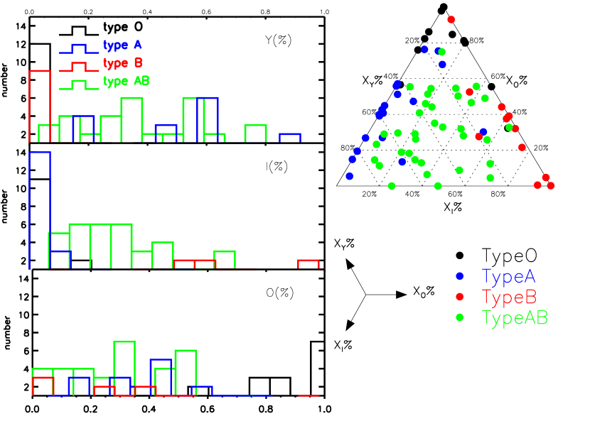
Figure 9: The age bin description was plotted in a trigonometric coordinate panel (right panel). black filled circles denote $typeO$, blue filled circles denote the $typeA$, red filled circles denote the $typeB$ and green filled circles denote the $typeAB$. The arrows in picture illustrate the direction to readout the $X_{Y}\%$, $X_{I}\%$, $X_{O}\%$, respectively. The same result are also depicted in the form of histograms (left panel). The black, blue, red and green histograms in each figure represent the $typeO$, $typeA$, $typeB$ and $typeAB$, respectively.

As discussed in Cid Fernandes et al. (2004), individual stellar population components are very uncertain because the existence of multiple solutions in stellar population and the further binning of the age will give a coarse but more robust description of the star formation history (SFH). We separate the stellar population into three components as suggested by Cid Fernandes et al. (2004): “young” ($X_{Y}$,$t\leq 1.0\times 10^{8}yr$), “intermediate” ($X_{I}$,$1.6\times 1.0^{8}yr\leq t\leq 1.27\times 10^{9}yr$) and “old” ($X_{O}$,$t\geq 1.43\times 10^{9}yr$). The diversity among four types objects is show in Figure 9, where we present a trigonometric coordinate of $X_{Y}+X_{I}+X_{O}=1$ panel. It is clear that the $typeO$ (black dot) is dominated by old age stellar population while the $typeA$ (blue dot) is dominated by young stars. $typrB$ (red dot) have a major contribution from intermediate population and the $typeAB$ (green dot) have mixed contribution from both young-aged and intermediate-aged stellar population, which is consistent with the result of composite spectra. To be more clearly, we depict the same result in the form of histograms (for each stellar population). The black, blue, red and green histograms in each figure represent the $typeO$, $typeA$, $typeB$ and $typeAB$, respectively.

4.2 AGN Luminosity Fraction and WISE Color

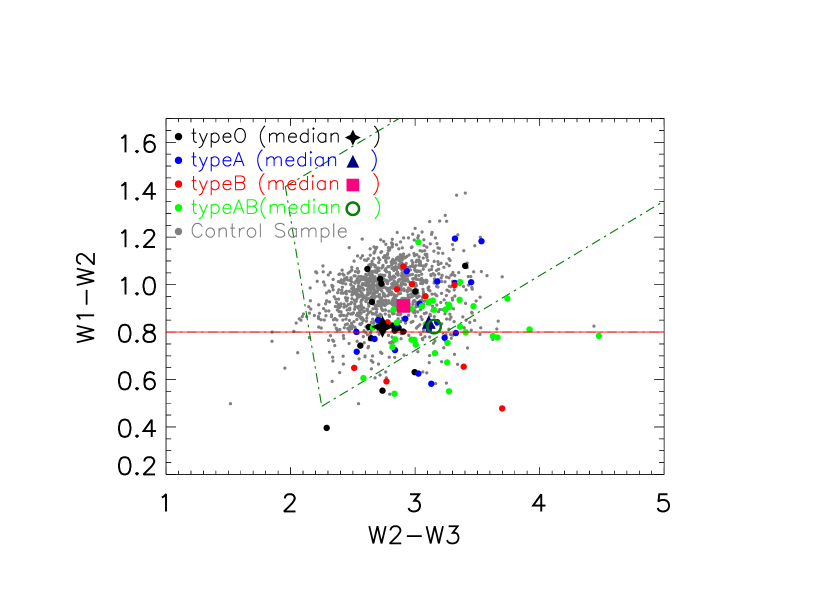
Figure 10: WISE colors of our working sample, which shows the $W1-W2\ vs\ W2-W3$: the meaning of the symbols are same as those in Figure 9 and the median value of each type are represented by different symbols (typeO: black star, typeA: blue taiangle, typeB: red square, typeAB: green open circle). There are different characteristic region used to select AGN. AGN wedge (dark green dot-dashed line) was defined by Mateos et al. (2012) and the mid-IR criteria (dark red dot-dashed line) was proposed by Stern et al. (2012).

The WISE has provided the data in the near- and mid-infrared. Stern et al. (2012) presented a simple mid-IR color criterion (W1-W2 $\geq$ 0.8) to identify AGN. Figure 10 shows the distribution of $W1-W2\ vs\ W2-W3$ for our 82 objects and the control sample. The median value of each type are also represented by different symbols (typeO: black star, typeA: blue taiangle, typeB: red square, typeAB: green open circle). As expected, most control sample have W1-W2 $\geq$ 0.8 (dark red solid line) while some objects of our working sample have W1-W2 bluer than 0.8. Stern et al. (2012) showed that a bluer W1-W2 is caused by host galaxy contamination in $z<2$. Additionally, the dark green dot-dashed line illustrates the selection of AGN using W1, W2 and W3 (Mateos et al., 2012). Not surprisingly, the sources in our working sample lie around AGN boundary with redder W2-W3 and bluer W1-W2. We give a Kolmogorov-Smirnov (KS) test between the working sample and control sample (Table 2). The result shows that the probabilities that the working sample and the control sample are drawn from the same distribution are $P_{KS}\ll 0.001$. The composite AGN/galaxy SED provided by Mateos et al. (2012) also suggested that the blend with host galaxy will lead the objects lie out the AGN wedge. Moreover, their work also show that the galaxy with old stellar content has W2-W3 color bluer than that of star-formation, which is consistent with our result: the W2-W3 color of $typeO$ and $typeB$ tend to be bluer than $typeA$ and $typeAB$ in color-color diagram. So we give a KS-test between $typeO+typeB$ and $typeA+typeAB$ in W23 and the resulting probability, $P_{KS}\ll 0.001$, suggests that they are come from different distribution.

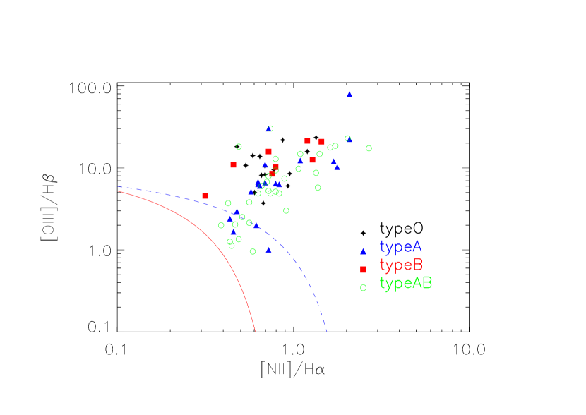
Figure 11: $[NII]/H{\alpha}$ versus $[OIII]/H{\beta}$ diagnostic diagram with line ratios and samples classified according to the combined classification scheme of Kewley et al. (2001) (blue dashed line) and Kauffmann et al. (2003) (red solid line). Each type are represented by different symbols (typeO: black star, typeA: blue triangle, typeB: red square, typeAB: green open circle).

The $[NII]/H\alpha$ versus $[OIII]/H\beta$ diagnostic diagram (BPT diagram) is commonly used to separate star formation from AGN activity (Baldwin et al., 1981; Veilleux & Osterbrock, 1987). The AGN sequence branches from the enriched end of the star-forming sequence and moves towards larger $[N_{II}]/H_{\alpha}$ and $[O_{III}]/H_{\beta}$ ratios as the AGN fraction increases. Wu et al. (2007) defined a quantity $d_{AGN}$ which measures the distance of galaxies from Kewley et al. (2001) theoretical upper bound of pure star formation, along lines parallel to the AGN sequence. Davies et al. (2014) also calculated relative AGN fractions by populating the composite region of BPT diagram with starburst-AGN mixing model. With the help of EW of narrow emission line from Shen et al. (2011), we plot our working sample in the BPT diagram (Figure 11). We observe a starburst-AGN mixing sequence of the working sample except $typeO$ exclusively occupy the region with high $frac_{AGN}$.

4.3 Correlation with AGN Properties

The tight correlation between the black hole and the bulge within which it resides ($M_{BH}\ vs\ M_{bulge}$, $L_{BH}\ vs\ L_{bulge}$, $M_{BH}\ vs\ \sigma_{bulge}$) reveals a close connection between black holes and their host galaxies. Heckman et al. (2004) found that in the most present-day accretion occurs onto black hole with masses less than $10^{8}M_{\odot}$ and young stellar population. In the study of (sub)mm-loud QSOs, Hao et al. (2008) found a trend that the star formation rate increases with the accretion rate. They also found the star formation rate decrease with the central black hole mass and suggested that the higher Eddington ratios of IR-QSOs imply that they are in the evolution stage toward QSOs. Heckman et al. (2004) found the similar result, at low redshift more massive galaxies tend to have older stellar population.

Shen et al. (2011) presented a compilation of properties of SDSS DR7 quasar catalog. In this product, they compiled continuum and emission measurements, as well as other quantities such as virial black hole mass and Eddington ratio estimates. With the help of these quasar properties, the expected correlations between AGN properties and stellar population are indeed found.

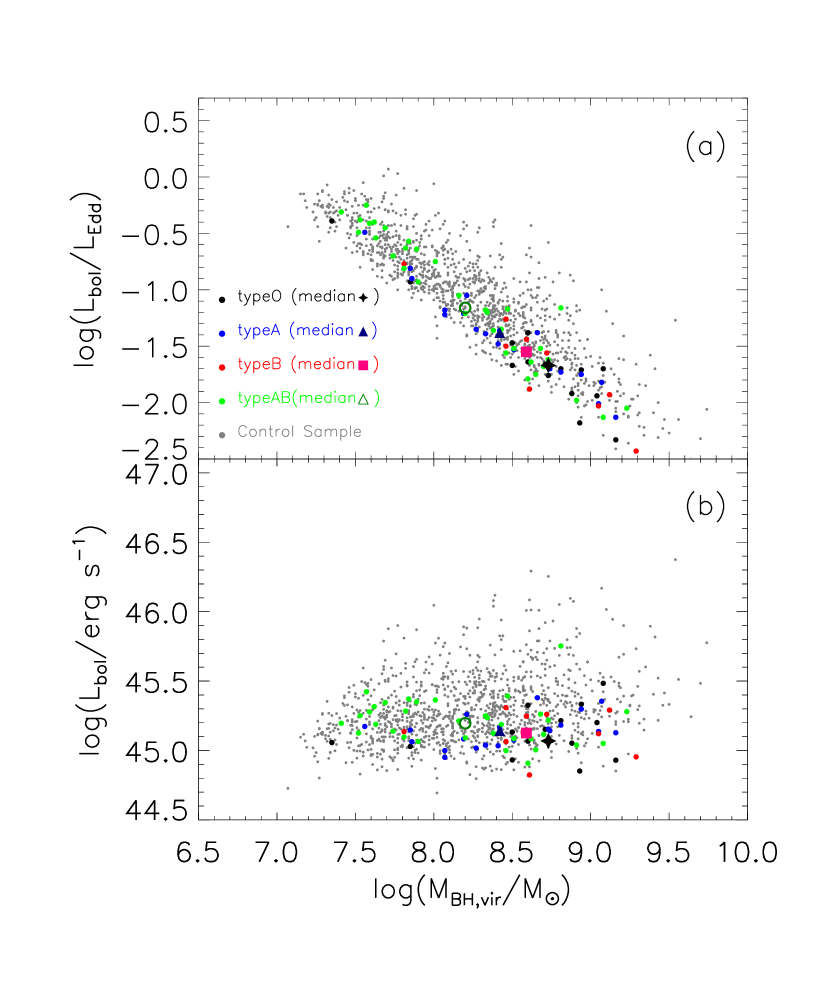
Figure 12: Panel (a) in Figure 12 shows the relation between $M_{BH,vir}$ and $L_{bol}/L_{Edd}$. The meaning of symbols are same as those in Figure 10. The panel (b) shows the relation between $M_{BH,vir}$ and $L_{bol}$.

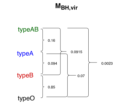
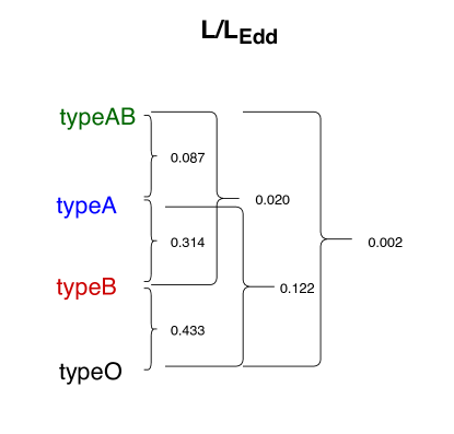
Figure 13: The result of KS-test for $M_{BH}$ and $L/L_{Edd}$: the probability of p value between any two types.

Panel (a) of Figure 12 shows a strong correlation between black hole mass and Eddington ratio ($M_{BH}$ increases as $L/L_{Edd}$ decreases) for the sources the working sample and control sample (gray dot). By applying the Pearson test, the statistical significance of this two variables is 0.001 and the correlation coefficient is 0.998, which means this two variables are related. Our result indicate that the low-mass black holes are more active than massive ones. In contrast, the more massive black holes are currently experiencing less additional accretion. The blue triangle, red square, green open circle and black star in Figure 12 denote the median value of $typeA$, $typeB$, $typeAB$ and $typeO$, respectively. By comparing these median value, we find that the QSOs with previous star formation activity ($typeA$, $typeB$ and $typeAB$) tend to have high Eddington ratio (stronger black hole active), statistically. Alternatively, the QSOs which have both former and recent star formation ($typeAB$) tend to have stronger AGN activity, while the $typeO$ which have no obvious star formation activity in the past are the inactive ones. Generally speaking, there may be correlation between the star formation and black hole activity, which may imply a co-evolution between SFH of host galaxies and AGN activity. The KS-test of both $M_{BH}$ and $L/L_{Edd}$ show that the working sample and the control sample are draw from the different distribution with $P_{KS}$ $\ll 0.001$. We also use the KS-test to test the significant difference of $M_{BH}$ and $L/L_{Edd}$ among these four types and the result are shown in Figure 13 (a) and (b), respectively. The number next to the braces gives the $P_{KS}$ of this two types. Combining with Figure 12, we can see that if the different between the median value of two types is greater, then the difference significance between these two type will also be greater (with small $P_{KS}$). The $P_{KS}$ between $typeAB$ (most active among four type) and $typeO$ (most inactive among four type) show that this two type are draw from the different distribution both in $M_{BH}$ and $L/L_{Edd}$.

Panel (b) of Figure 12 shows a relationship between black holes mass and luminosity of the working sample. We quantify the Eddington and BH masses by calculating their mean values and standard errors (SE) for all four types and the control sample (Table 3). Compared with control QSOs, our working sample seems have lower Eddington ratio as well as lower luminosity which may be result from the selection effect (the high luminosity QSOs tend to have a more powerful AGN and may overwhelm the light of host galaxies). The KS-test of luminosity show that the working sample and the control sample are draw from the different distribution with $P_{KS}$ $\ll 0.001$.

4.4 Interaction of host galaxies

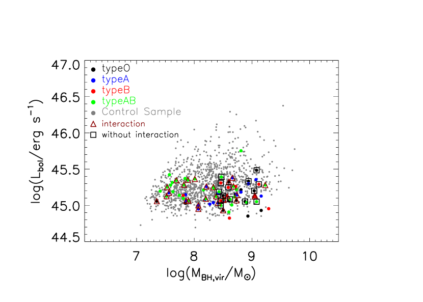
Figure 14: The interaction condition of host galaxies were ploted on the program of $M_{BH}\ vs\ L_{bol}$. The black squares represent the host galaxies without interaction while the red triangles represent the host galaxies with obvious tidal feature. The meaning of other symbols are same as those in previous figure.

A long term discussion concerning the properties of the galaxies hosting QSOs is its morphology. To study the host galaxy morphology properties and their interaction, we use images from the SDSS. The main challenge in understanding the host galaxy is the poor spatial resolution of the ground-based observations and combined with the bright nuclei hindered the nature of the QSOs host. We just classify our sources into tow types: Y(30) with obvious interactivity, which was represented with red triangle in Figure 14 and N (14) which don’t shows any tidal feature and no companion (black squares). The rest 38 source is hard to be classified by SDSS image. It is interesting that the host galaxies without interaction are exclusive locate in high black hole mass and alliance with $typeO$ and $typeB$ (9/14). This result may indicate that objects without recent star formation and high black hole mass may already relax from the interactivation and evolve to the quiescent ellipse galaxies.

5 Discussion

By studying the stellar population of host galaxies in type I QSOs among different SFH types, we find that the stellar population is associated with the AGN physical properties. These result is consistent with the finding of Sanders et al. (1988) and Gebhardt et al. (2000) , at least some QSOs are in the advanced merge stage.

5.1 Spectral comparison between our working sample and others

Sanders et al. (1988) suggested a evolutionary sequence from ULIRGs to QSOs. Hao et al. (2005) and Cao et al. (2008) also proposed that at last some IR-QSOs are at a transitional stage from ULIRGs to classical QSOs. The work of Treister et al. (2012) showed that most luminous AGN (QSOs, $M_{R}\leq-22$) seem to be triggered by major mergers. If so, the composite spectra of the working sample will be consistent with the idea that they are hybrids of AGN and starbursts (or post-starbust ). We compare different kind of spectra in Figure 8. As we can see in panel (a), the spectra of QSOs from Shang et al. (2011) (both radio quiet and radio loud) are brighter in the wavelength shorter than 5100$\AA$ and even much brighter than control sample. It may because most objects selected from Shang et al. (2011) are UV-bright-AGN. The ULIRGs have roughly similar SED to the starburst galaxies while IR-QSOs is more bright in the shorter wavelength, which are consistent with the evolutionary mentioned before. Additionally, the spectra of our working sample is closed to PSQs from Cales et al. (2011), which means they have similar $frac_{AGN}$ or even in the similar evolution stage. The study of Cales et al. (2011) shows that the PSQs have a starburst within  100 Myr which is smaller than our age range. Combined with the analysis in $Section\ 4.1$, our objects may in the evolutionary stage from IR-QSOs to typical optical QSOs.

5.2 The AGN properties in the evolution

In former analysis, we find a compelling correlation between the star-busts (both former dramatically enhanced and recent moderate star formation) and AGN properties. Considering the typical QSOs’ lifetime are expected to be $\sim 10^{8}$ yr, the dramatically enhanced star formation can’t have been triggered at the same time as they occurred few hundred Myr ago. However, there are some theories can explain the correlation between black hole activity and former star formation (Canalizo & Stockton, 2000; Walter et al., 2002; Hutchings et al., 2003; Granato et al., 2004; Hopkins et al., 2006; Letawe et al., 2007; Cox et al., 2008; Hopkins, 2012).

The previous work suggested that star-burst may occur at the early stage of merger or interaction, when the AGN has not been triggered yet and then followed by decrease in accretion of AGN with the aging of stellar content (Canalizo & Stockton, 2000; Granato et al., 2004; Hopkins et al., 2006). Hopkins (2012) showed that such a time delay can occur for purely dynamical reasons. His simulations showed firstly the gas move toward center and gives rise to the star formation. Then, the gas flowing further inwards by losing angular momentum and produces a time delay between star formation and AGN activity. What’s more, many numerical simulations show that the star formation as well as AGN activity is episodic (Hopkins et al., 2008; Van Wassenhove et al., 2012; Torrey et al., 2012), which depend on the detail of the merge (orbits, morphological type of progenitors). In this picture, the former dramatically enhanced star formation of QSO hosts in the working sample are induced in the early stages of galaxies merger. As the galaxies continue to merge for next few hundred Myr, the gas flowing further inwards central regions, followed by the AGN activity. The recent moderate star formation in our working sample may be triggered by a minor merge due the accretion of a satellite (Cox et al., 2008). Many works (Walter et al., 2002; Hutchings et al., 2003; Letawe et al., 2007) suggest that minor merger that do not produce dramatically enhanced star formation, while still fuelling the AGN. Our result is consistent with that of the former work. Davies et al. (2007) analyzed the star formation in the nuclei of nine Seyfert galaxies, which also show a possible starbursts in the last 10-300 Myr. In the work of Schawinski et al. (2009), the AGN (obscured and unobscured) appear to be prevalent in the ”green valley” on the color-magnitude diagram. They suggested that there is a  100Myr time delay between the shutdown of star formation and detectable AGN. The research of Heckman et al. (2004) also used type 2 AGNs to investigate the accretion-driven growth of super-massive black holes and found that bulge formation and black hole formation are tightly coupled in present-day. The study of Santini et al. (2012); Floyd et al. (2013) shows a higher SFRs of AGN host galaxies than that of inactive galaxies with the same stellar mass and redshift.

6 Summary

We have studies the stellar population of 82 host galaxies of type I QSOs selected from the cross-matched SDSS DR7 QSOs and WISE catalog with the S/N of stellar content great than 15. Our method is a powerful technique for selecting the type I QSOs with obvious host component and investigating the properties of their host galaxies. Compared with WISE color and BPT diagram, we have shown that this technique can efficiently separate the spectroscopic components and give a reliably stellar content and $frac_{AGN}$. Furthermore, we can also classify our working sample into four type by SFH ($typeO$, $typeA$, $typeB$ and $typeAB$) of host with this method.

The composite spectra, age distribution and WISE color-color diagram show that:(1) the stellar population have a significant contribution to the observed emission in our sources; (2) The $typeO$ are dominated by older stellar content; $typeA$ are dominated by young stellar content; the $typeB$ are dominated by intermediate stellar content; $typeAB$ have a mixed component of young and intermediate stellar content.

Considering the AGN properties such as black hole mass and Eddington ratio, we suggest that there is a co-evolution between AGN and host galaxies. Our result also shows there is a time delay between the peak of star formation and black hole accretion and then both of them decrease slowly. In addition, the host galaxies that do not show sign of interactive ( no tidal feature and companion galaxies ) are exclusive reside in the object with big black hole mass and relative old stellar population and imply they are the object relaxed form interactive. Most of our sources may be in the transition phase from IR-QSOs to classical optical QSOs.

Figure 4: $\chi^{2}/N_{\lambda}$vs $frac_{AGN}$. The left panel is the example for adopting minimal $\chi^{2}/N_{\lambda}$ as best fitting value; The right panel is the example for adopting averaged $\chi^{2}/N_{\lambda}$ as best fitting value.

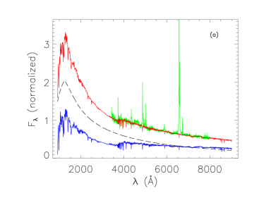
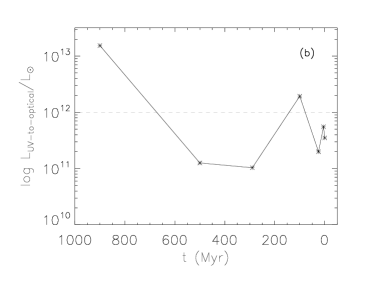
Figure 6: Panel (a) shows the rebuilt model spectrum (red solid line) of SDSS J153705.95+005522.8, which is superimposed by the observed one (green solid), the host galaxy spectrum (blue solid line) as well as the power-law spectrum (black dashed line). Panel (b) shows the SFH of the same host galaxy.

Table 1: The main parameter of of our source. (1) SDSS ID; (2-3) coordinates (4) redshift (5) WISE magnitude (6) Interaction

SDSS_name	ra	dec	z	W1	W2	W3	W4	Interaction
101405.89+000620.3	10:14:06	+00:06:22	0.140	11.639	10.573	7.956	5.899
111807.47+002734.9	11:18:07	+00:27:36	0.168	13.623	13.227	10.930	7.876
113021.41+005823.0	11:30:21	+00:58:23	0.132	12.514	11.696	8.829	6.232
112852.59-032130.5	11:28:53	-03:21:29	0.197	13.516	12.705	8.786	6.661
125933.48-012833.3	12:59:34	-01:28:34	0.266	13.154	12.260	9.108	6.595	Y
171411.63+575833.9	17:14:12	+57:58:34	0.092	11.439	10.544	7.717	5.248
025938.15+004216.3	02:59:38	+00:42:18	0.195	13.678	13.128	9.856	7.348
080037.62+461257.9	08:00:38	+46:12:58	0.238	13.309	12.403	9.127	6.478	Y
090906.40+535040.4	09:09:06	+53:50:42	0.273	13.826	13.115	9.956	7.826
034831.88-071145.9	03:48:32	-07:11:46	0.183	12.591	11.640	8.557	6.055	N
090158.88+002313.8	09:01:59	+00:23:13	0.196	12.818	11.885	8.743	6.213	Y
111713.91+674122.7	11:17:14	+67:41:24	0.247	12.697	11.695	8.721	6.323	N
131953.15+033335.9	13:19:53	+03:33:36	0.208	13.577	12.995	9.865	7.857
133715.92+030936.5	13:37:16	+03:09:36	0.192	13.328	12.574	9.314	7.085
150420.90+015159.3	15:04:21	+01:51:58	0.182	12.958	11.960	8.644	6.068
075057.26+353037.6	07:50:57	+35:30:36	0.175	13.355	12.172	8.639	6.327
082405.19+445246.0	08:24:05	+44:52:44	0.219	13.397	12.456	8.715	6.604
104451.87+035251.9	10:44:52	+03:52:52	0.206	13.291	12.482	9.372	7.209
151600.39+572415.7	15:16:00	+57:24:14	0.204	12.948	12.108	9.255	6.878
162633.92+480230.1	16:26:34	+48:02:31	0.242	12.904	11.977	8.869	6.666	N
003657.17-100810.6	00:36:57	-10:08:10	0.187	13.208	12.554	9.164	6.627	N
033156.88+002605.2	03:31:57	+00:26:06	0.236	13.602	12.761	9.982	7.696
113630.11+621902.4	11:36:30	+62:19:01	0.211	13.511	12.715	9.388	6.832	Y
083453.39+384708.5	08:34:53	+38:47:10	0.184	13.445	12.611	9.759	7.746
083917.34+392817.9	08:39:17	+39:28:19	0.186	13.182	12.376	9.540	7.285
133706.93+051803.3	13:37:07	+05:18:04	0.163	13.820	13.342	9.643	6.762	Y
081116.70+320935.3	08:11:17	+32:09:36	0.153	12.544	11.743	9.215	6.648	Y
110051.02+513502.1	11:00:51	+51:35:02	0.213	13.254	12.452	9.547	7.350	N
123915.40+531414.6	12:39:15	+53:14:13	0.201	12.999	12.407	9.637	7.070	Y
081835.59+390911.1	08:18:36	+39:09:11	0.186	13.623	12.804	10.140	7.488	N
132832.58-023321.4	13:28:33	-02:33:22	0.183	12.955	12.349	9.764	7.200	N
134452.60-011452.2	13:44:53	-01:14:53	0.177	13.210	12.443	9.449	6.786
081438.27+290619.9	08:14:38	+29:06:22	0.225	13.565	12.646	9.609	7.017
105705.40+580437.4	10:57:06	+58:04:37	0.140	12.514	11.889	8.863	6.736	Y
131750.32+601040.8	13:17:50	+60:10:41	0.136	12.180	11.324	8.403	5.799	Y
133237.93+593053.6	13:32:38	+59:30:54	0.171	12.234	11.466	8.495	5.927	Y
133435.38+575015.6	13:34:35	+57:50:17	0.123	12.309	11.411	8.442	6.038
171756.03+261148.6	17:17:56	+26:11:49	0.145	13.791	13.022	10.180	7.919	N
152008.23+461615.3	15:20:08	+46:16:16	0.176	13.491	12.748	10.180	8.176	Y
134615.88+580008.1	13:46:16	+58:00:07	0.162	12.936	12.199	9.381	6.576
151907.33+520605.9	15:19:07	+52:06:07	0.137	11.042	9.848	6.528	3.947	Y
154518.05+463837.9	15:45:18	+46:38:38	0.228	11.385	10.328	7.395	4.752	Y
093302.68+385228.0	09:33:03	+38:52:26	0.177	12.450	11.618	8.532	6.363	Y
100302.15+095832.8	10:03:02	+09:58:34	0.253	13.420	12.416	9.687	7.535	N
125908.35+561530.7	12:59:08	+56:15:32	0.160	12.371	11.444	8.791	6.214
143123.52+392501.4	14:31:24	+39:25:01	0.161	13.349	12.718	9.722	7.479
113651.66+445016.4	11:36:52	+44:50:17	0.115	12.302	11.630	8.373	6.254
135719.47+394045.3	13:57:19	+39:40:44	0.265	13.566	12.767	9.361	7.381
140007.29+405357.6	14:00:07	+40:53:56	0.167	12.891	12.117	9.471	6.807	Y
105409.18+412827.6	10:54:09	+41:28:26	0.230	14.781	14.057	11.210	8.469
112930.76+431017.3	11:29:31	+43:10:16	0.186	13.282	12.729	9.991	7.636	N
091020.11+312417.8	09:10:20	+31:24:18	0.265	13.666	12.751	9.480	7.043	Y
114926.47+112629.0	11:49:26	+11:26:28	0.177	12.941	12.119	9.490	7.690	N
121945.03+082117.9	12:19:45	+08:21:18	0.228	13.144	12.133	8.772	6.095	Y
155654.47+253233.6	15:56:54	+25:32:35	0.164	13.253	12.604	10.090	7.629	Y
155958.01+261102.7	15:59:58	+26:11:02	0.228	13.374	12.465	9.411	6.869	Y
160700.93+245056.6	16:07:01	+24:50:56	0.183	12.720	11.707	8.529	5.977	Y
132105.98+504634.4	13:21:06	+50:46:34	0.233	12.881	11.945	8.588	6.320
141557.25+495334.5	14:15:57	+49:53:35	0.185	13.558	12.781	9.119	6.612	Y
134704.91+144137.6	13:47:05	+14:41:38	0.134	12.509	11.614	8.370	5.828
151453.27+053636.8	15:14:53	+05:36:36	0.173	12.844	11.934	9.030	6.464
080652.11+564412.7	08:06:52	+56:44:13	0.180	12.027	10.848	7.822	5.476	Y
100208.14+345353.7	10:02:08	+34:53:53	0.205	12.718	11.642	8.736	6.284	N
122028.07+405035.0	12:20:28	+40:50:35	0.221	12.955	12.129	9.306	7.021	Y
130712.33+340622.5	13:07:12	+34:06:22	0.147	12.686	11.607	8.205	5.422
115515.86+380234.9	11:55:16	+38:02:35	0.143	12.825	11.983	8.806	6.404	Y
115828.53+373450.1	11:58:29	+37:34:52	0.186	13.824	13.041	9.416	7.038	Y
121006.01+333602.9	12:10:06	+33:36:04	0.225	13.364	12.513	9.810	7.512
135852.46+295413.1	13:58:53	+29:54:14	0.113	11.426	10.446	7.591	5.128
142230.34+295224.2	14:22:30	+29:52:23	0.113	12.789	12.005	7.529	4.402	Y
151337.07+201133.6	15:13:37	+20:11:35	0.270	12.932	11.961	8.959	6.438	N
161002.70+202108.5	16:10:03	+20:21:07	0.217	13.166	12.419	9.414	7.149	N
110805.03+271313.9	11:08:05	+27:13:16	0.358	13.148	12.221	9.325	7.133
091848.61+211717.0	09:18:49	+21:17:17	0.149	11.063	10.039	7.320	4.824	Y
102955.58+244523.2	10:29:56	+24:45:22	0.220	13.789	13.018	10.340	7.848	Y
115248.18+212255.5	11:52:48	+21:22:55	0.171	13.108	12.568	9.734	7.408	Y
154526.04+141159.3	15:45:26	+14:12:00	0.284	13.552	12.545	9.226	6.692
132954.86+182041.7	13:29:55	+18:20:42	0.188	13.266	12.490	9.253	6.827
150408.46+143123.3	15:04:08	+14:31:23	0.118	11.667	10.657	7.207	4.914	Y
153031.25+120734.0	15:30:31	+12:07:34	0.197	13.517	12.800	10.260	8.115
152205.06+012626.6	15:22:05	+01:26:28	0.113	11.871	10.962	7.493	5.045
153705.95+005522.8	15:37:06	+00:55:23	0.136	12.497	11.674	8.314	6.232

Table 2: The KS-test of WISE color.

type	W12	W23
Working sample vs Control	$\ll 0.001$	$\ll 0.001$
typeO+typeB vs typeA+typeAB		$\ll 0.001$

Table 3: The mean values with standard errors of BH mass and Eddington ratio for four types and control sample.

		logBH		logEdd
type	mean	standard errors	mean	standard errors
typeO	8.65	0.12	-1.63	0.12
typeA	8.45	0.10	-1.41	0.09
typeB	8.67	0.13	-1.60	0.15
typeAB	8.20	0.09	-1.09	0.10
control sample	8.23	0.02	-0.56	0.02

References

- Aird et al. (2010) Aird, J., Nandra, K., Laird, E. S., et al. 2010, MNRAS, 401, 2531
- Assef et al. (2013) Assef, R. J., Stern, D., Kochanek, C. S., et al. 2013, ApJ, 772, 26
- Baldwin et al. (1981) Baldwin, J. A., Phillips, M. M., & Terlevich, R. 1981, PASP, 93, 5
- Barnes & Hernquist (1991) Barnes, J. E., & Hernquist, L. E. 1991, ApJ, 370, L65
- Barnes & Hernquist (1992) Barnes, J. E., & Hernquist, L. 1992, ARA&A, 30, 705
- Barnes & Hernquist (1996) Barnes, J. E., & Hernquist, L. 1996, ApJ, 471, 115
- Barth et al. (2008) Barth, A. J., Bentz, M. C., Greene, J. E., & Ho, L. C. 2008, ApJ, 683, L119
- Blank & Duschl (2016) Blank, M., & Duschl, W. J. 2016, MNRAS, 462, 2246
- Bruzual & Charlot (2003) Bruzual, G., & Charlot, S. 2003, MNRAS, 344, 1000
- Caccianiga et al. (2015) Caccianiga, A., Antón, S., Ballo, L., et al. 2015, MNRAS, 451, 1795
- Cales et al. (2011) Cales, S. L., Brotherton, M. S., Shang, Z., et al. 2011, ApJ, 741, 106
- Cales et al. (2013) Cales, S. L., Brotherton, M. S., Shang, Z., et al. 2013, ApJ, 762, 90
- Cales & Brotherton (2015) Cales, S. L., & Brotherton, M. S. 2015, MNRAS, 449, 2374
- Calzetti et al. (2000) Calzetti, D., Armus, L., Bohlin, R. C., et al. 2000, ApJ, 533, 682
- Canalizo et al. (2000) Canalizo, G., Stockton, A., Brotherton, M. S., & van Breugel, W. 2000, AJ, 119, 59
- Canalizo & Stockton (2000) Canalizo, G., & Stockton, A. 2000, AJ, 120, 1750
- Canalizo & Stockton (2013) Canalizo, G., & Stockton, A. 2013, ApJ, 772, 132
- Canalizo & Stockton (2001) Canalizo, G., & Stockton, A. 2001, ApJ, 555, 719
- Cao et al. (2006) Cao, C., Wu, H., Wang, J.-L., et al. 2006, Chinese J. Astron. Astrophys., 6, 197
- Cao et al. (2008) Cao, C., Xia, X. Y., Wu, H., et al. 2008, MNRAS, 390, 336
- Charlot & Bruzual (2007) Charlot, S. & Bruzual, G. 2007,models distributed on demand (CB07)
- Cid Fernandes et al. (2004) Cid Fernandes, R., Gu, Q., Melnick, J., et al. 2004, MNRAS, 355, 273
- Cid Fernandes et al. (2005) Cid Fernandes, R., Mateus, A., Sodré, L., Stasińska, G., & Gomes, J. M. 2005, MNRAS, 358, 363
- Clements et al. (1996) Clements, D. L., Sutherland, W. J., McMahon, R. G., & Saunders, W. 1996, MNRAS, 279, 477
- Cox et al. (2008) Cox, T. J., Jonsson, P., Somerville, R. S., Primack, J. R., & Dekel, A. 2008, MNRAS, 384, 386
- Cui et al. (2001) Cui, J., Xia, X.-Y., Deng, Z.-G., Mao, S., & Zou, Z.-L. 2001, AJ, 122, 63
- Davies et al. (2007) Davies, R. I., Müller Sánchez, F., Genzel, R., et al. 2007, ApJ, 671, 1388
- Davies et al. (2014) Davies, R. L., Kewley, L. J., Ho, I.-T., & Dopita, M. A. 2014, MNRAS, 444, 3961
- Di Matteo et al. (2005) Di Matteo, T., Springel, V., & Hernquist, L. 2005, Nature, 433, 604
- Ferrarese & Merritt (2000) Ferrarese, L., & Merritt, D. 2000, ApJ, 539, L9
- Jahnke et al. (2007) Jahnke, K., Wisotzki, L., Courbin, F., & Letawe, G. 2007, MNRAS, 378, 23
- Kauffmann et al. (2003) Kauffmann, G., Heckman, T. M., Tremonti, C., et al. 2003, MNRAS, 346, 1055
- Kewley et al. (2001) Kewley, L. J., Dopita, M. A., Sutherland, R. S., Heisler, C. A., & Trevena, J. 2001, ApJ, 556, 121
- Kennicutt (1992) Kennicutt, R. C., Jr. 1992, ApJS, 79, 255
- Kim et al. (2002) Kim, D.-C., Veilleux, S., & Sanders, D. B. 2002, ApJS, 143, 277
- Kormendy & Richstone (1995) Kormendy, J., & Richstone, D. 1995, ARA&A, 33, 581
- Kormendy & Gebhardt (2001) Kormendy, J., & Gebhardt, K. 2001, 20th Texas Symposium on relativistic astrophysics, 586, 363
- Kormendy & Sanders (1992) Kormendy, J., & Sanders, D. B. 1992, ApJ, 390, L53
- Dunlop et al. (2003) Dunlop, J. S., McLure, R. J., Kukula, M. J., et al. 2003, MNRAS, 340, 1095
- Engel et al. (2010) Engel, H., Davies, R. I., Genzel, R., et al. 2010, A&A, 524, A56
- Farrah et al. (2001) Farrah, D., Rowan-Robinson, M., Oliver, S., et al. 2001, MNRAS, 326, 1333
- Fitzpatrick (1999) Fitzpatrick, E. L. 1999, PASP, 111, 63
- Ferrarese & Merritt (2000) Ferrarese, L., & Merritt, D. 2000, ApJ, 539, L9
- Floyd et al. (2013) Floyd, D. J. E., Dunlop, J. S., Kukula, M. J., et al. 2013, MNRAS, 429, 2
- Gebhardt et al. (2000) Gebhardt, K., Bender, R., Bower, G., et al. 2000, ApJ, 539, L13
- Gebhardt et al. (2000) Gebhardt, K., Kormendy, J., Ho, L. C., et al. 2000, ApJ, 543, L5
- Granato et al. (2004) Granato, G. L., De Zotti, G., Silva, L., Bressan, A., & Danese, L. 2004, ApJ, 600, 580
- Gunn et al. (2006) Gunn, J. E., Siegmund, W. A., Mannery, E. J., et al. 2006, AJ, 131, 2332
- Hao et al. (2005) Hao, C. N., Xia, X. Y., Mao, S., Wu, H., & Deng, Z. G. 2005, ApJ, 625, 78
- Hao et al. (2008) Hao, C.-N., Xia, X.-Y., Shu-DeMao, Deng, Z.-G., & Wu, H. 2008, Chinese J. Astron. Astrophys., 8, 12
- Hatziminaoglou et al. (2008) Hatziminaoglou, E., Fritz, J., Franceschini, A., et al. 2008, MNRAS, 386, 1252
- Heckman et al. (2004) Heckman, T. M., Kauffmann, G., Brinchmann, J., et al. 2004, ApJ, 613, 109
- Hopkins (2004) Hopkins, A. M. 2004, ApJ, 615, 209
- Hopkins et al. (2006) Hopkins, P. F., Hernquist, L., Cox, T. J., Robertson, B., & Springel, V. 2006, ApJS, 163, 50
- Hopkins et al. (2008) Hopkins, P. F., Hernquist, L., Cox, T. J., & Kereš, D. 2008, ApJS, 175, 356-389
- Hopkins (2012) Hopkins, P. F. 2012, MNRAS, 420, L8
- Hutchings et al. (2003) Hutchings, J. B., Maddox, N., Cutri, R. M., & Nelson, B. O. 2003, AJ, 126, 63
- Larson & Tinsley (1978) Larson, R. B., & Tinsley, B. M. 1978, ApJ, 219, 46
- Letawe et al. (2007) Letawe, G., Magain, P., Courbin, F., et al. 2007, MNRAS, 378, 82
- Maraston (2005) Maraston, C. 2005, MNRAS, 362, 799
- Mateos et al. (2012) Mateos, S., Alonso-Herrero, A., Carrera, F. J., et al. 2012, MNRAS, 426, 3271
- Magain et al. (1998) Magain, P., Courbin, F., & Sohy, S. 1998, ApJ, 494, 472
- Magorrian et al. (1998) Magorrian, J., Tremaine, S., Richstone, D., et al. 1998, AJ, 115, 2285
- McLure et al. (1999) McLure, R. J., Kukula, M. J., Dunlop, J. S., et al. 1999, MNRAS, 308, 377
- Meng et al. (2010) Meng, X.-M., Wu, H., Gu, Q.-S., Wang, J., & Cao, C. 2010, ApJ, 718, 928
- Meng et al. (2011) Meng, X.-M., Wu, H., & Cao, C. 2011, Research in Astronomy and Astrophysics, 11, 419
- Merritt & Ferrarese (2001) Merritt, D., & Ferrarese, L. 2001, MNRAS, 320, L30
- Moustakas & Kennicutt (2006) Moustakas, J., & Kennicutt, R. C., Jr. 2006, ApJS, 164, 81
- Murphy et al. (1996) Murphy, T. W., Jr., Armus, L., Matthews, K., et al. 1996, AJ, 111, 1025
- Nolan et al. (2001) Nolan, L. A., Dunlop, J. S., Kukula, M. J., et al. 2001, MNRAS, 323, 308
- Rembold et al. (2017) Rembold, S. B., Shimoia, J. S., Storchi-Bergmann, T., et al. 2017, MNRAS, 472, 4382
- Richards et al. (2002) Richards, G. T., Fan, X., Newberg, H. J., et al. 2002, AJ, 123, 2945
- Rieke & Low (1972) Rieke, G. H., & Low, F. J. 1972, ApJ, 176, L95
- Rieke & Lebofsky (1979) Rieke, G. H., & Lebofsky, M. J. 1979, ARA&A, 17, 477
- Sánchez et al. (2004) Sánchez, S. F., Jahnke, K., Wisotzki, L., et al. 2004, ApJ, 614, 586
- Sánchez et al. (2018) Sánchez, S. F., Avila-Reese, V., Hernandez-Toledo, H., et al. 2018, Rev. Mexicana Astron. Astrofis., 54, 217
- Sanders & Mirabel (1996) Sanders, D. B., & Mirabel, I. F. 1996, ARA&A, 34, 749
- Sanders et al. (1988) Sanders, D. B., Soifer, B. T., Elias, J. H., et al. 1988, ApJ, 325, 74
- Sanders et al. (1988) Sanders, D. B., Soifer, B. T., Elias, J. H., Neugebauer, G., & Matthews, K. 1988, ApJ, 328, L35
- Shang et al. (2011) Shang, Z., Brotherton, M. S., Wills, B. J., et al. 2011, ApJS, 196, 2
- Santini et al. (2012) Santini, P., Rosario, D. J., Shao, L., et al. 2012, A&A, 540, A109
- Schawinski et al. (2009) Schawinski, K., Virani, S., Simmons, B., et al. 2009, ApJ, 692, L19
- Schlegel et al. (1998) Schlegel, D. J., Finkbeiner, D. P., & Davis, M. 1998, ApJ, 500, 525
- Schneider et al. (2010) Schneider, D. P., Richards, G. T., Hall, P. B., et al. 2010, AJ, 139, 2360
- Shen et al. (2011) Shen, Y., Richards, G. T., Strauss, M. A., et al. 2011, ApJS, 194, 45
- Silverman et al. (2008) Silverman, J. D., Green, P. J., Barkhouse, W. A., et al. 2008, ApJ, 679, 118-139
- Springel et al. (2005) Springel, V., Di Matteo, T., & Hernquist, L. 2005, MNRAS, 361, 776
- Stern et al. (2012) Stern, D., Assef, R. J., Benford, D. J., et al. 2012, ApJ, 753, 30
- Stoughton et al. (2002) Stoughton, C., Lupton, R. H., Bernardi, M., et al. 2002, AJ, 123, 485
- Tadhunter et al. (2005) Tadhunter, C., Robinson, T. G., González Delgado, R. M., Wills, K., & Morganti, R. 2005, MNRAS, 356, 480
- Taniguchi (1999) Taniguchi, Y. 1999, ApJ, 524, 65
- Toomre & Toomre (1972) Toomre, A., & Toomre, J. 1972, ApJ, 178, 623
- Toomre (1977) Toomre, A. 1977, ARA&A, 15, 437
- Tremaine et al. (2002) Tremaine, S., Gebhardt, K., Bender, R., et al. 2002, ApJ, 574, 740
- Treister et al. (2012) Treister, E., Schawinski, K., Urry, C. M., & Simmons, B. D. 2012, ApJ, 758, L39
- Torrey et al. (2012) Torrey, P., Cox, T. J., Kewley, L., & Hernquist, L. 2012, ApJ, 746, 108
- Vanden Berk et al. (2001) Vanden Berk, D. E., Richards, G. T., Bauer, A., et al. 2001, AJ, 122, 549
- Vanden Berk et al. (2006) Vanden Berk, D. E., Shen, J., Yip, C.-W., et al. 2006, AJ, 131, 84
- Van Wassenhove et al. (2012) Van Wassenhove, S., Volonteri, M., Mayer, L., et al. 2012, ApJ, 748, L7
- Veilleux & Osterbrock (1987) Veilleux, S., & Osterbrock, D. E. 1987, ApJS, 63, 295
- Veilleux et al. (2002) Veilleux, S., Kim, D.-C., & Sanders, D. B. 2002, ApJS, 143, 315
- Voit (1992) Voit, G. M. 1992, MNRAS, 258, 841
- Walter et al. (2002) Walter, F., Weiss, A., Martin, C., & Scoville, N. 2002, AJ, 123, 225
- Wild et al. (2010) Wild, V., Heckman, T., & Charlot, S. 2010, MNRAS, 405, 933
- Wei et al. (2013) Wei, P., Shang, Z., Brotherton, M. S., et al. 2013, ApJ, 772, 28
- Wold et al. (2010) Wold, I., Sheinis, A. I., Wolf, M. J., & Hooper, E. J. 2010, MNRAS, 408, 713
- Wright et al. (2010) Wright, E. L., Eisenhardt, P. R. M., Mainzer, A. K., et al. 2010, AJ, 140, 1868-1881
- Wu et al. (1998a) Wu, H., Zou, Z. L., Xia, X. Y., & Deng, Z. G. 1998, A&AS, 127, 521
- Wu et al. (1998b) Wu, H., Zou, Z. L., Xia, X. Y., & Deng, Z. G. 1998, A&AS, 132, 181
- Wu et al. (2007) Wu, H., Zhu, Y.-N., Cao, C., & Qin, B. 2007, ApJ, 668, 87
- Xia et al. (2002) Xia, X. Y., Xue, S. J., Mao, S., et al. 2002, ApJ, 564, 196
- Yesuf et al. (2014) Yesuf, H. M., Faber, S. M., Trump, J. R., et al. 2014, ApJ, 792, 84
- York et al. (2000) York, D. G., Adelman, J., Anderson, J. E., Jr., et al. 2000, AJ, 120, 1579
- Zibetti et al. (2013) Zibetti, S., Gallazzi, A., Charlot, S., Pierini, D., & Pasquali, A. 2013, MNRAS, 428, 1479
- Zhang-hu & Qiu-sheng (2016) Zhang-hu, C., & Qiu-sheng, G. 2016, Chinese Astron. Astrophys., 40, 291
- Zheng et al. (1999) Zheng, Z., Wu, H., Mao, S., et al. 1999, A&A, 349, 735
- Zou et al. (1991) Zou, Z., Xia, X., Deng, Z., & Su, H. 1991, MNRAS, 252, 593