A long-term alternative formula for a stochastic stock price model

Abstract

This study presents a long-term alternative formula for stock price variation described by a geometric Brownian motion on the basis of median instead of mean or expected values. The proposed method is motivated by the observation made in remote fields, where optimality of bet-hedging or diversification strategies is explained based on a measure different from expected value, like geometric mean. When the probability distribution of possible outcomes is significantly skewed, it is generally known that expected value leads to an erroneous picture owing to its sensitivity to outliers, extreme values of rare occurrence. Since geometric mean, or its counterpart median for the log-normal distribution, does not suffer from this drawback, it provides us with a more appropriate measure especially for evaluating long-term outcomes dominated by outliers. Thus, the present formula makes a more realistic prediction for long-term outcomes of a large volatility, for which the probability distribution becomes conspicuously heavy-tailed.

MSC Classification] 91Bxx,91B06,91B62,62P05,62P20

Article Highlights

• We call into question the validity of expected value concept applied to heavy-tailed distributions of stock prices

• We propose an alternative formula for evaluating future prices based on median

• The proposed idea is in line with biological bet-hedging and the Kelly criterion in optimal betting

1 Introduction

The Black-Scholes-Merton (BSM) theory has been considered the standard model of prices in financial markets black73 ; merton73 . The Black-Scholes (BS) formula gives the price of a European call option, i.e., the right to buy a stock on a future day. This formula is derived under the assumptions of the BSM theory, i.e, a constant riskless rate, a geometric Brownian motion with constant drift and volatility, no dividends, no arbitrage opportunity, no commissions and transactions costs, and a frictionless market hull18 . Although the BSM theory has been generally successful and widely accepted, some shortcomings of the BS formula, including the long-term prediction, have become clear over the past decades. Many models have been introduced to overcome the shortcomings originating from the assumptions of the BSM theory hull18 . Among others, a local volatility model dupire94 and stochastic volatility models heston93 ; gatheral06 are important generalizations to relax the assumption of constant volatility. While these specific points should be addressed on their merits, the purpose of the present study is to approach from a more general perspective to this matter. We cast doubt on a methodological presupposition in deriving the stock price formula, that is, the practicality of the fundamental concept in probability theory, the expected value. In short, we question if the expected value is really expected. In various fields facing similar issues, it is generally acknowledged that the expected value of random variables can happen to deviate significantly from a middle of the distribution owing to its strong dependence on outliers, i.e., extremely large values that occur with extremely small probabilities. This strong dependence may cause a serious bias toward the overestimation of what is actually expected. In particular, expected value should deviate appreciably from the expectation of market participants, because the future value of stock prices is almost certainly plagued with outliers. Nonetheless, expected value is undoubtedly a key concept in economics and finance. Thus, we find it worthwhile to seek knowledge from remote fields where this problematic situation has been coped with.

In social and behavioural sciences, it is well known that there are cases in which expected value leads to an erroneous result. For instance, a centuries-old thought experiment of the St. Petersburg paradox should be mentioned bernoulli38 . While the expected value of payoffs is infinite, rational people will not pay more than a few times as large as the smallest payoff martin17 . The point here is just as mentioned above, i.e., the expected value has a drawback of overestimating the extreme events of rare occurrence. More specifically, there are abundant examples on this matter in the field of ecological biology. The number of a population under stochastic environments varies in a similar fashion as stock prices. It is widely acknowledged that the geometric mean of growth rates (geometric mean fitness) lewontin69 provides a more satisfactory picture of population growth yoshimura91 ; clark00 , than the arithmetic mean, i.e., the expected value. Risk-spreading or bet-hedging strategies of animals are a concrete example that is understood by means of geometric mean fitness yasui18 , but not with expected value. The geometric mean concept is intimately related to the median of growth rates, as exemplified for the St. Petersburg Paradox okabe19 . The present work is motivated from this observation made in these fields remote from finance.

The structure of the remainder of this paper is as follows. In Section 2, we highlight the motivational background by means of a multiplicative growth model. This is instructive in two respects. Firstly, temporal variation of stock prices is described by a similar model. Secondly, this model has already been widely used in ecology of the population growth under uncertain environments lewontin69 , as well as in mathematics of optimal strategy in repeated gambles thorp . The basic idea behind the prior studies is to use the geometric mean of randomly varying quantities as a proper measure. In Section 3, we discuss the stock price model of a geometric Brownian motion to derive the geometric-mean counterpart, i.e., median, of the stock price formula. The main result is given in Eq. (2). Section 4 provides the numerical results obtained by computer simulation as a concrete example to support the main point of using median in place of expected value. Section 5 gives discussions. Section 6 gives conclusions and future research.

2 Background

The stochastic behavior of stock price is mathematically modelled as a geometric Brownian motion (GBM) bachelier00 and it has since long been utilized for a wide application kanagawa05 . Most notably, the BSM theory has been considered the standard model of prices in financial markets black73 ; merton73 . Before discussing the GBM model, we explain the basic idea of the present study based on a simpler model.

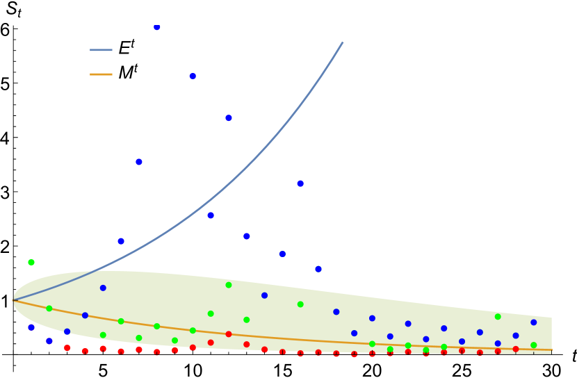
Figure 1: Temporal variation of size $S_{t}$ in a stochastic multiplicative growth model. The exponential growths by the mean $E$ and the median $M$ are contrasted. Dots indicate three realizations of the stochastic process. The values within the shaded area account for 68% of the data set (either of the two growth rates $l_{1}=0.5$ and $l_{2}=1.7$ occurs with a 50% probability).

In the multiplicative growth model, we suppose that population size $S_{t}$ at time $t$ grows geometrically, i.e., it varies in the multiplicative manner $S_{t+1}=l_{t}S_{t}$. The growth rates $l_{t}$ at discrete times $t=0,1,2,\cdots$ form a sequence of independent, identically distributed random variables, i.e., each obeys the same probability distribution. In population ecology, Lewontin and Cohen used this model to discuss population growth under randomly varying environments lewontin69 . Around the same time, essentially the same argument was made in a different context of repeated bets (gambles), i.e., in what is called today the Kelly criterion thorp . If the rates at different times are independent of each other, the expected value of $S_{t}$ is given by $E[S_{t}]=(\mu_{l})^{t}S_{0}$, where $\mu_{l}=E[l_{t}]$ is the mean (expected value) of $l_{t}$. If the mean is greater than unity ($\mu_{l}>1$), one would expect that the size $S_{t}$ blows up as $t$ grows. However, this expectation may be subverted almost certainly. For example, when $l_{t}$ comprises two possibilities $l=0.5$ and $l=1.7$ occurring with equal probability, we have $\mu_{l}=1.1$ so that the expected size grows as $E[S_{100}]=1.1^{100}S_{0}=13781S_{0}$. Nevertheless, as a matter of fact, the probability that the final size $S_{100}$ surpasses the original value $S_{0}$ is very small (Prob$[S_{100}>S_{0}]=0.092$) (Fig. 1). Therefore, contrary to the expectation, population size is almost certain to vanish ($S_{100}\simeq 0$). This paradox is caused by skewness, or asymmetry, of the probability distribution above and below the mean (the expected value). In fact, the cumulative probability above the mean is significantly smaller than that below (Prob$[S_{t}>E[S]]=0.022$ and Prob$[S_{t}<E[S]]=0.978$). In this problem, a more satisfactory solution is provided by the geometric mean $G=e^{\mu_{\log l}}$ ($S_{t}\simeq G^{t}S_{0}$), rather than by the expected value $\mu_{l}=E[S_{t}]$ ($S_{t}\simeq\mu_{l}^{t}S_{0}$). Note that the geometric mean $\sqrt[n]{l_{1}l_{2}\cdots l_{n}}$ of $l_{1},l_{2},\cdots,l_{n}$ is the arithmetic mean in logscale, i.e., $e^{\frac{1}{n}\sum_{i}\log l_{i}}$. Hence, $G=e^{\mu_{\log l}}$ is the geometric mean. Since $\mu_{\log l}=-0.08126<0$, we obtain $G\simeq 0.92$, and the most typical behavior is the exponential decay $S_{100}\simeq 0.92^{100}S_{0}$, instead of the exponential blow-up $1.1^{100}S_{0}$ expected from the expected value. In fact, it is straightforward to see that $M=G^{t}S_{0}$ is the median of $S_{t}$ (see Appendix A). We present this example to underscore the antinomy that the epected value $E[S_{t}]=\mu_{l}^{t}S_{0}$ inflates while the median $M=G^{t}S_{0}$ deflates (Fig. 1). In this antinomy, the latter provides us with a typical behavior of our expectation in the sense that the latter (median) is almost certain to occur while the former (expected value) is little expected (with a 2.2% probability).

3 Model and Results

In the multiplicative model, the geometric mean of randomly varying growth rates corresponds to the median of their probability distribution. This is generally true for the random variable obeying the lognormal distribution. Thus, we can make a parallel argument for stock prices because they follow the same distribution, the lognormal distribution.

In the BSM model, the market consists of a risky asset (stock $S$) and a riskless asset (bond $B$). The former obeys the stochastic differential equation $dS_{t}=\mu S_{t}dt+\sigma S_{t}dW_{t}$, where $dW_{t}$ is a stochastic variable hobson04 . The latter varies as $B_{t}=B_{0}e^{rt}$ with $B_{0}=1$. Since the logarithm of the stock price $S_{t}$ discounted by $B_{t}$ follows a normal distribution, the terminal stock price $S_{T}$ follows the log-normal distribution $f_{S_{T}}(x)$, i.e., $\log S_{T}$ obeys the normal distribution with mean $\log S_{0}+(r-\sigma^{2}/2)T$ and variance $\sigma^{2}T$, where $T$ is the time to maturity. For the strike price $K$, the BS formula for the price of a European call option is given by

$$C_{BS}(S_{0},K,T) = {e^{-rT}}{\rm max}(E[S_{T}]-K,0)$$ (1)

$$= e^{-rT}\int_{K}^{\infty}(S_{T}-K)f_{S_{T}}(x)dx$$

$$= S_{0}\Phi(d_{1})-e^{-rT}K\Phi(d_{2}),$$

where $d_{1}=(\log(S_{0}/K)+(r+\sigma^{2}/2)T)/(\sigma\sqrt{T})$ and $d_{2}=d_{1}-\sigma\sqrt{T}$ hull18 . In a similar manner, it is straightforward to obtain the median counterpart. Noting that the median of the log-normal distribution $f_{S_{T}}(x)$ is given by the exponentiated mean, $S_{0}\exp(rT-\sigma^{2}T/2)$, we obtain

$$C={\rm max}\left(S_{0}\exp(-\sigma^{2}T/2)-e^{-rT}K,0\right),$$ (2)

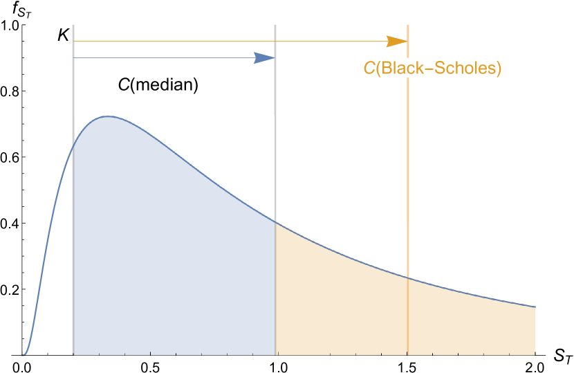
Figure 2: The median $C$ and the mean $C_{BS}$ (Black-Scholes). The probability distribution of price $S_{T}$ ($S_{0}=1.5,\sigma=1,T=1,r=0$ and $K=0.2$).

i.e., $C=0$ for $K>S_{0}\exp((r-\sigma^{2}/2)T)$ and $C=S_{0}\exp(-\sigma^{2}T/2)-e^{-rT}K$ otherwise (Fig.2). This is the main result of the present study. It should be remarked that analytical results are available for the expected value as well as the median because the model leads to the log-normal distribution. This is not necessarily the case for sophisticated models to take into account practical factors.

In the above, we presented a standard method of deriving the BS formula in which the behavior of stock prices is modelled with the stochastic differential equation of a geometric Brownian motion. Another original method is based on solving a diffusion partial differential equation, the Black-Scholes equation hull18 . The latter method does not serve the present purpose, not only because it does not deal with individual processes but the use of expected value is implicitly taken for granted while referring to a mathematical result on the diffusion equation.

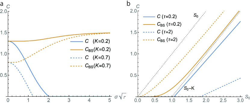
Figure 3: The median $C$ and the mean $C_{BS}$ (Black-Scholes). a, $C$ and $C_{BS}$ for $K=0.2$ and 0.7 are plotted against $\sigma\sqrt{T}$ ($S_{0}=1.5$ and $r=0$). b, $C$ and $C_{BS}$ for $T=0.2$ and $T=2$ are plotted against $S_{0}$ ($r=0.2$, $K=1$ and $\sigma=1$). The BS formula $C_{BS}$ gives concave curves between $S_{0}$ and $S_{0}-K$.

Generally speaking, the alternative formula $C$ falls below $C_{BS}$, occasionally significantly, owing to the insensitivity to the extreme events of rare occurrence that affect the latter. The two formulae $C_{BS}$ and $C$ give the same result in the shortest term, i.e., $C_{BS}=C$ at $T=0$. However, they make strikingly different long-term predictions (Fig. 3a). As the time $T$ increases, $C_{BS}$ increases continuously to the stock price $S_{0}$, independently of $K$ black73 ; merton73 . This is not the case for $C$. Accordingly, the $S_{0}$-dependence of $C$ is modified drastically (Fig.3b). The difference is because the probability above the mean of the log-normal distribution drops exponentially as $\Phi(-\sigma\sqrt{T}/2)$ while the median of the log-normal distribution is independent of $T$. Thus, the present formula resolves the discrepancy between expected value and typical value that becomes appreciable in the long-time behaviour, while it coincides with the original result in case where their difference does not stand out.

4 Simulated data

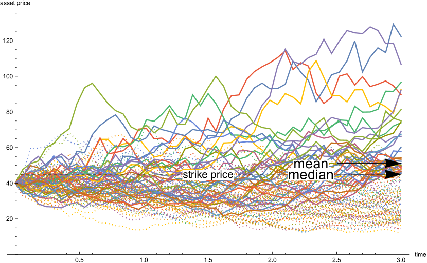
Figure 4: Temporal variation of stock price $S_{t}$ as simulated by geometric Brownian motion (GBM) paths (starting price $S_{0}=40$, strike price $K=45$, maturity time $T=3$, stock price volatility $\sigma=0.3$, risk-free interest rate $r=0.07$, stock dividend yield $\delta=0$, and the number of time steps is 50). Among the total of 100 simulated paths, 67 paths end up with $S_{T}<K$, which are displayed with dotted lines. An arrow with "mean" signifies the discounted mean of the option’s payoffs at expiry. An arrow with "median" is the median counterpart.

To support the present method, we show numerical results simulated based on geometric Brownian motion (GBM) paths (Fig. 4). If we denote as $S_{j,t}$ the stock price at the $t$-th time grid of the $j$-th path, the BS result is given by the mean of the option value at maturity, $e^{-rT}{\rm max}({E}[S_{j,n}]-K,0)$, where ${E}[S_{j,n}]=\frac{1}{m}\sum_{j=1}^{m}S_{j,n}$. Note that $m$ and $n$ are the number of GBM paths and that of time steps, respectively ($S_{j,1}=S_{0}$ and $S_{j,n}=S_{T}$ for the $j$-th path). In Fig. 4, this result is indicated with an arrow labeled with mean. For comparison, the result by the proposed method, the median of the option value at maturity, is indicated with an arrow labeled with median.

For the sake of illustration, we present $m=100$ paths of price variation in Fig. 4. As shown with dotted lines, more than two thirds (67 out of 100) end up with no value ($S_{j,n}<K$). Thus, the median (no value) is more than twice as likely to result than any positive value. It is important to remark that about half of the mean value $C_{BS}=6.2$ (i.e., 2.9) comes just from the 5 largest outcomes with $S_{T}>80$ (standing out in Fig.4). We emphasize that these results are typically expected unless volatility $\sigma$ is assumed negligibly small and the time $n$ to the maturity is too short. The more we increase the path number $m$, the more conspicuously the probability to end up with no value increases. Accordingly, the probability to obtain ‘lucky’ results to make a major contribution to the expected value, becomes negligibly small. Under these circumstances, the median formula is more appropriate and realistic than with the expected value approach.

5 Discussions

The BS formula is most often used to calculate the market implied volatility, which is a forward-looking measure that captures the market’s view of the likelihood of changes in an option price. Most of the assumptions in its evaluation are embedded in the option pricing model, while others like the target of the present study originate from methodological presumptions. The present study is aimed at shedding light on the assumption of the latter kind. The expected value concept does not properly take account of the likelihood aspect of unevenly distributed outcomes. The main purpose of this study is to underline the importance of this aspect, a deep-rooted problem unquestioned so far, by way of presenting the new formula. In this sense, the present interest is more of a scientific nature than a practical one. We aimed at confronting the inadequacy of the expected value $E(S_{t})$ when there is an exponential discrepancy in the ratio of probabilities above and below it, namely Prob[$S_{t}>E(S_{t})$] and Prob[$S_{t}<E(S_{t})$]. In practice, notable differences between theoretical and real values are empirically corrected by introducing ad-hoc parameters as called ’implied volatility’ and previous studies have obtained satisfactory results with generalized models while based on the expected value concept hull18 .

In probability theory, the expected value (mean, average) is known to be away from most typical outcomes when the probability distribution has a large skew or includes a few extreme outliers. Here the median is much closer to these typical outcomes than the mean. Thus, the alternative median formula gives a better estimate for the call options when there are outliers or large skews, e.g., the subprime mortgage crisis in 2007-2008 hull18 . Recently, the log-normal distribution used for stock prices is questioned and the probability distribution of stock prices have been estimated from the past records using, for example, the boot-strap model instead hull18 . We should note that the assumption of the lognormal distribution can be replaced to such a practical distribution to gain the better results to avoid the problem of the abovementioned statistical outliers. In practice, extreme events of a heavy-tailed distribution may have substantial impacts in many stochastic dynamical systems, including economical buldyrev11 , and other social ones newman . While it is often hardly possible to quantify them with mathematical rigor, it is still very important to have a practical scheme as proposed presently that takes account of the possible effect of extreme events.

6 Conclusion

Motivated by bet-hedging strategies in evolutionary ecology and optimal betting by means of the Kelly criterion, the present study proposes a new conservative long-term formula for the stochastic model of stock prices, which is based on the median of the log-normal distribution of future stock prices. The presented formula has an advantage over the conventional one in that it is insensitive to extremely large values that can be theoretically possible but practically almost impossible. We focused on a European call option to underline the practical feasibility of the proposed approach. Future research directions include a put option, American options, and the delta of an option hull18 , which are immediate, and also other fields to deal with exponential stochastic processes, where a long-term measure is required for sustainable development.

Appendix A Median of the log-normal distribution

We consider $\log S_{t}=\log S_{0}+\sum_{t=0}^{t-1}\log l_{t}$, where $l_{t}$ at $t=0,1,2,\cdots$ form a sequence of independent, identically distributed random variables. If we denote mean and variance of $\log l_{t}$ as $\mu_{\log l}$ and $\sigma_{\log l}^{2}$, respectively, the central limit theorem states that the mean $\frac{1}{t}\sum_{t=0}^{t-1}\log l_{t}$ for a large $t$ follows the normal distribution with mean $\mu_{\log l}$ and variance $\sigma_{\log l}^{2}/t$. In orther words, $S_{t}$ is distributed according to a log-normal distribution. Accordingly, the probability of $S_{t}$ being less than $K$ is given in terms of the cumulative distribution function of the standard normal distribution (with mean 0 and standard deviation 1), $\Phi(y)=\frac{1}{\sqrt{2\pi}}\int_{-\infty}^{y}e^{-t^{2}/2}dt$, i.e.,

$${\rm Prob}[S_{t}<K]={\rm Prob}\left[\frac{1}{t}\sum_{t=0}^{t-1}\log l_{t}<\frac{1}{t}\log\frac{K}{S_{0}}\right]=\Phi\left(\frac{\frac{1}{t}\log\frac{K}{S_{0}}-\mu_{\log l}}{\sigma_{\log l}/\sqrt{t}}\right).$$

The median $M$ is given by the value of $K$ to make this probability equal to 1/2, that is, $M=S_{0}(e^{\mu_{\log l}})^{t}$. The quantity in the parentheses ($G=e^{\mu_{\log l}}$) is the geometrical mean of $l$. It should be mentioned that not only the median but other quartiles may serve the present purpose. In order to meet the expectation of market participants, the representative measure should always keep a moderate value to the probability of getting $K$ or more, ${\rm Prob}[S_{t}>K]=1-{\rm Prob}[S_{t}<K]$. The expected value $K=E$ is defective in that it makes this probability depend on $t$ and vanish exponentially as $t$ increases. A rational person would find little value in anything with an exponentially small probability.

Compliance with Ethical Standards

This work was partly supported by grants-in-aid from the Japan Society for Promotion of Science (no. 21K12047 to TO). The authors have no relevant financial or non-financial interests to disclose. This article does not contain any studies with human participants or animals performed by any of the authors.

The authors have no conflict of interest to disclose. No datasets were analysed during the current study.

References

- (1) Black F, Scholes M (1973) The Pricing of Options and Corporate Liabilities. Journal of Political Economy 81: 637-654. https://doi.org/10.1086/260062
- (2) Merton RC (1973) Theory of Rational Option Pricing. The Bell Journal of Economics and Management Science 4: 141-183. https://doi.org/10.2307/3003143
- (3) Hull JC (2022) Options, Futures, and Other Derivatives, 11th Edition, Pearson.
- (4) Dupire B (1994) Pricing with a smile. Risk 7: 18-20.
- (5) Heston SL (1993) A Closed-Form Solution for Options with Stochastic Volatility with Applications to Bond and Currency Options. The Review of Financial Studies 6: 327-343. http://dx.doi.org/10.1093/rfs/6.2.327
- (6) Gatheral J (2006) The Volatility Surface - A Practitioner’s Guide, Wiley.
- (7) Bernoulli D (1954) Specimen theoriae novae de mensura sortis (Exposition of a new theory on the measurement of risk), Transl. by Sommer, L. Econometrica 22: 23-36. https://doi.org/10.2307/1909829
- (8) Martin R (2017) The St. Petersburg paradox, in Edward N.Zalta (Ed.), The Stanford Encyclopedia of Philosophy, Winter, https://plato.stanford.edu /archives /win2017/entries/paradox-stpetersburg/
- (9) Lewontin RC, Cohen D (1969) On Population Growth In A Randomly Varying Environment, Proceedings of the National Academy of Sciences 62: 1056-1060. https://doi.org/10.1073/pnas.62.4.1056
- (10) Yoshimura J, Clark CW (1991) Individual adaptations in stochastic environments. Evolutionary Ecology 5: 173-192. https://doi.org/10.1007/BF02270833
- (11) Clark CW, Mangel M (2000) Dynamic State Variable Models in Ecology: Methods and Applications, Oxford University Press
- (12) Yasui Y (2022) Evolutionary bet-hedging reconsidered: What is the mean-variance trade-off of fitness? Ecological Research 37: 406-420. https://doi.org/10.1111/1440-1703.12303
- (13) Okabe T, Nii M, Yoshimura J (2019) The median-based resolution of the St. Petersburg paradox. Physics Letters A 383: 125838 https://doi.org/10.1016/j.physleta.2019.125838
- (14) Bachelier L (1900) Théorie de la spéculation, Annales Scientifiques de l’École Normale Supérieure 3: 21-86. https://doi.org/10.24033/asens.476
- (15) Kanagawa S, Arimoto A, Saisho Y (2005) Numerical simulation of multi dimensional reflecting geometrical Brownian motion and its application to mathematical finance, Nonlinear Analysis: Theory, Methods & Applications 63: e2209-e2222. https://doi.org/10.1016/j.na.2005.02.076
- (16) Thorp, E.O. (1969) Optimal Gambling Systems for Favorable Games, Review of the International Statistical Institute, 37: 273-293. https://doi.org/10.2307/1402118
- (17) Hobson D (2004) A survey of mathematical finance. Proceedings of the Royal Society A 460: 3369-3401. https://doi.org/10.1098/rspa.2004.1386
- (18) Buldyrev SV, Flori A, Pammolli F (2011) Market instability and the size-variance relationship. Scientific Reports 11: 5737. https://doi.org/10.1038/s41598-021-84680-1
- (19) Newman MEJ (2005) Power laws, Pareto distributions and Zipfs law. Contemporary Physics 46: 323-351. https://doi.org/10.1080/00107510500052444