QCD evolution based evidence for the onset of gluon saturation in exclusive photo-production of vector mesons

Abstract

We investigate photo-production of vector mesons $J/\Psi$ and $\Upsilon$ measured both at HERA and LHC, using 2 particular fits of inclusive unintegrated gluon distributions, based on non-linear Balitsky-Kovchegov evolution (Kutak-Sapeta gluon; KS) and next-to-leading order Balitsky-Fadin-Kuraev-Lipatov evolution (Hentschinski-Sabio Vera-Salas gluon; HSS). We find that linear next-to-leading order evolution can only describe production at highest energies, if perturbative corrections are increased to unnaturally large values; rendering this corrections to a perturbative size, the growth with energy is too strong and the description fails. At the same time, the KS gluon, which we explore both with and without non-linear corrections, requires the latter to achieve an accurate description of the energy dependence of data. We interpret this observation as a clear signal for the presence of high gluon densities in the proton, characteristic for the onset of gluon saturation.

1 Introduction

Energies available at the LHC allow for a detailed study of dynamical effects of Quantum Chromodynamics (QCD). A prominent example is the Heavy Ion program which focuses on the study of the Quark Gluon Plasma (QGP). While many of the QGP properties are understood, the initial state leading to its formation poses still open questions [1, 2]. A closely related question is the formation of an over occupied system of gluons, which eventually leads to saturation of gluon densities [3]; finding convincing phenomenological evidence for gluon saturation is still one of the open problems of QCD. On microscopic level, gluon saturation is expected to arise as a consequence of recombination of so-called wee gluons. The net effect of such recombination is to slow down the growth of gluon number density with energy, commonly referred to as gluon saturation. The evolution from the low to large gluon densities is described by a set of nonlinear evolution equations, known as Balitsky-Jalilian-Marian-Iancu-McLerran-Weigert-Leonidov-Kovner evolution [4, 5, 6]; its frequent used mean field version is given by the Balitsky Kovchegov (BK) [4, 7] evolution equation. First hints for gluon saturation could be already found in data collected from HERA experiments [8], (for a review see: [9] and references therein). More recent studies focus on resolving hadronic final states at RHIC and LHC to explore the transverse momentum distribution in the potentially saturated proton and nucleus, e.g. hadron production [10, 13, 11, 14, 12] or azimuthal de-correlations of dijets [15]. Such studies allow to study signals of saturation linked indirectly to the energy dependence of gluon distributions.

In contrast to these studies, exclusive production of vector mesons provides a direct opportunity to explore the energy dependence of the cross section [16, 17, 18]. Since for this observable large amount of data on production of $J/\Psi,\Upsilon(1S)$ has been collected over wide range of energies, it allows to potentially observe the predicted slow down of the growth with energy of cross-sections, which is one of the core predictions associated with the presence of high and saturated gluon densities. Studies in the literature for this process, which take into account effects due to gluon saturation, exist both on the level of dipole models [16, 17, 18, 19, 20] and complete solutions to non-linear BK equation [21, 22]. The description of the cross sections is in general satisfactory. Here we would like to re-investigate the problem from a different angle: While the ability of non-linear evolution equations to describe collider data is a necessary requirement to establish the presence of gluon saturation, it is not sufficient: albeit a successful description of data is provided, one might still remain in the so-called dilute regime, where gluon densities are perturbative. That this could be actually the case, is at least suggested by the successful description of the same data set by frameworks which rely on collinear factorization [23, 24, 25, 26] and – maybe even more striking – linear NLO BFKL evolution [27]. The latter relies on a fit of an initial (low energy) transverse momentum distribution to combined HERA data by Hentschinski-Salas-Sabio Vera (HSS)[28], and has been recently explored in a number of phenomenological studies, see e.g. [29].

In the following we will argue that even though a description of exclusive photo-production data by linear QCD evolution can be achieved for the entire range of available center-of-mass energies, such a description requires unnaturally large higher order corrections, which in some region of phase space are larger than the dominant leading order term. To assess the importance of non-linear terms in low $x$ evolution equations, we use a particular solution to BK-evolution, with initial conditions fitted to combined HERA data by Kutak-Sapeta (KS) [30]. While the HSS-gluon relies on NLO-BKFL evolution and KS-evolution on LO-BK evolution, both evolution schemes supplement the original low $x$ evolution with a supplementary resummation of collinear logarithms [31]. Our strategy is then as follows: While exclusive photo-production of the $\Upsilon$ serves as the necessary cross-check in the perturbative, dilute region (provided by the relatively large bottom quark mass), saturation effects will be searched for in photo-production of the $J/\Psi$ mesons (where the hard scale is provided by the charm quark mass). In particular we will demonstrate that the seemingly flawless description of $J/\Psi$-data by NLO BFKL evolution is only possible due to the presence of a very large perturbative correction, which slows down the growth with energy. Choosing on the other hand a hard scale which renders this perturbative corrections small, the data are no longer described. The KS gluon (which is subject to non-linear QCD evolution) is on the other hand able to describe the energy dependence of $J/\Psi$-data. Turning off the non-linear effects in the evolution of the KS-gluon, we find that a description of the energy dependence is no longer possible. We are convinced that this observation provides a very strong phenomenological evidence for the presence of saturation effects in the high $W$ region of $J/\Psi$ photo-production observed at the LHC.

The outline of this letter is as follows: In Sec. 2 we provide details of our theoretical description, Sec. 3 is dedicated to a discussion of the large perturbative corrections of the NLO BFKL gluon in the large $W$ region while in Sec. 4 we present our conclusions.

2 Energy dependence of the photo-production cross-section

We study the process $\gamma(q)+p(p)\to V(q^{\prime})+p(p^{\prime})$ where $V=J/\Psi,\Upsilon(1S)$ and $\gamma$ denotes a quasi-real photon with virtuality $Q\to 0$; $W^{2}=(q+p)^{2}$ is the squared center-of-mass energy of the $\gamma(q)+p(p)$ collision. The $x$ value probed in such a collision is obtained as $x\simeq M_{V}^{2}/W^{2}$ with $M_{V}$ the mass of the vector meson. With the momentum transfer $t=(q-q^{\prime})^{2}$, the differential cross-section for the exclusive production of a vector meson can be written in the following form

$$\frac{d\sigma}{dt}\left(\gamma p\to Vp\right) =\frac{1}{16\pi}\left|\mathcal{A}_{T,L}^{\gamma p\to Vp}(W^{2},t)\right|^{2}\,,$$ (1)

where $\mathcal{A}(W^{2},t)$ denotes the scattering amplitude for the reaction $\gamma p\to Vp$ for color singlet exchange in the $t$-channel, with an overall factor $W^{2}$ already extracted. For a more detailed discussion of the kinematics we refer to [27].

2.1 The theoretical setup of our study

In the following we determine the total photo-production cross-section, based on an inclusive gluon distribution. This is possible following a two step procedure, frequently employed in the literature: First one determines the differential cross-section at zero momentum transfer $t=0$ (which can be expressed in terms of the inclusive gluon distribution); in a second step the $t$-dependence is modeled which then allows us to relate the differential cross-section at $t=0$ to the integrated cross-section. Here we follow the prescription given in [23, 24], where an exponential drop-off with $|t|$, $\sigma\sim\exp\left[-|t|B_{D}(W)\right]$ is used with an energy dependent $t$ slope parameter $B_{D}$, as motivated by Regge theory,

$$B_{D}(W) =\left[b_{0}+4\alpha^{\prime}\ln\frac{W}{W_{0}}\right]\text{GeV}^{-2}.$$ (2)

Following [23, 24], we use for the numerical values $\alpha^{\prime}=0.06$ GeV^-2, $W_{0}=90$ GeV and $b_{0}^{J/\Psi}=4.9$ GeV^-2 in the case of the $J/\Psi$, while $b_{0}^{\Upsilon}=4.63$ GeV^-2 for $\Upsilon$ production. The total cross-section for vector meson production is therefore obtained as

$$\sigma^{\gamma p\to Vp}(W^{2}) =\frac{1}{B_{D}(W)}\frac{d\sigma}{dt}\left(\gamma p\to Vp\right)\bigg{|}_{t=0}.$$ (3)

The uncertainty introduced by the modeling of the $t$-dependence mainly affects the overall normalization of the cross-section with a mild logarithmic dependence on the energy. To determine the scattering amplitude, we first note that the dominant contribution is provided by its imaginary part. Corrections due to the real part of the scattering amplitude can be estimated using dispersion relations, in particular

$$\frac{\Re\text{e}\mathcal{A}(W^{2},t)}{\Im\text{m}\mathcal{A}(W^{2},t)} =\tan\frac{\lambda\pi}{2}, \lambda =\frac{d\ln\Im\text{m}\mathcal{A}(W^{2},t)}{d\ln W^{2}}\,.$$ with (4)

As noted in [27, 32], the dependence of the slope parameter $\lambda$ on energy $W$ provides a sizable correction to the $W$ dependence of the complete cross-section. We therefore do not assume $\lambda=$ const., but instead determine the slope $\lambda$ directly from the $W$-dependent imaginary part of the scattering amplitude. The latter is obtained from [20, 19]

$$\Im\text{m}\mathcal{A}^{\gamma p\rightarrow Vp}_{T}(W,t=0) =2\,\int\!d^{2}{\bm{r}}\int\!d^{2}{\bm{b}}\int_{0}^{1}\!\frac{d{z}}{4\pi}\;(\Psi_{V}^{*}\Psi)_{T}\;\mathcal{N}\left(x,r,b\right)\,,$$ (5)

where $\mathcal{N}\left(x,r,b\right)$ is the dipole amplitude and $T$ denotes transverse polarization of the quasi-real photon. Here

$$\left(\Psi_{V}^{*}\Psi\right)_{T}(r,z) =\frac{\hat{e}_{f}eN_{c}}{\pi z(1-z)}\bigg{\{}m_{f}^{2}K_{0}(\epsilon r)\phi_{T}(r,z)-\left[z^{2}+(1-z)^{2}\right]\epsilon K_{1}(\epsilon r)\partial_{r}\phi_{T}(r,z)\bigg{\}}\,,$$ (6)

with $\epsilon^{2}=m_{f}^{2}$ for real photons. Furthermore $r=\sqrt{{\bm{r}}^{2}}$, while $f=c,b$ denotes the flavor of the heavy quark and $\hat{e}_{f}=2/3$, $-1/3$. For the scalar parts of the wave functions $\phi_{T,L}(r,z)$, we employ the boosted Gaussian wave-functions with the Brodsky-Huang-Lepage prescription [33]. For the ground state vector meson ($1s$) the scalar function $\phi_{T}(r,z)$, has the following general form [20, 34],

$$\phi_{T,L}^{1s}(r,z) =\mathcal{N}_{T,L}z(1-z)\exp\left(-\frac{m_{f}^{2}\mathcal{R}_{1s}^{2}}{8z(1-z)}-\frac{2z(1-z)r^{2}}{\mathcal{R}_{1s}^{2}}+\frac{m_{f}^{2}\mathcal{R}_{1s}^{2}}{2}\right)\,.$$ (7)

The free parameters $N_{T}$ and $\mathcal{R}_{1s}$ of this model have been determined in various studies from the wave function normalization and the decay width of the vector mesons. In the following we use the values found in [16] ( $J/\Psi$) and [18] ( $\Upsilon$). The parameters are summarized in Tab. 1.

Meson	$m_{f}/\text{GeV}$	$\mathcal{N}_{T}$	$\mathcal{R}^{2}$/$\text{GeV}^{-2}$	$M_{V}$/GeV
$J/\psi$	$m_{c}=1.4$	$0.596$	$2.45$	$3.097$
$\Upsilon$	$m_{b}=4.2$	$0.481$	$0.57$	$9.460$

Table 1: Parameters of the boosted Gaussian vector meson wave functions for $J/\psi$ and $\Upsilon$ [16, 18].

In the forward limit $t=0$, one further has,

$$2\int d^{2}{\bm{b}}\,\mathcal{N}\left(x,r,b\right) =\sigma_{q\bar{q}}(x,r)\,,$$ (8)

where $\sigma_{q\bar{q}}$ denotes the inclusive dipole cross-section which is related to the unintegrated gluon density ${\cal F}$ through [35]

$$\sigma_{q\bar{q}}(x,r) =\frac{4\pi}{N_{c}}\int\frac{d^{2}{\bm{k}}}{{\bm{k}}^{2}}\left(1-e^{i{\bm{k}}\cdot{\bm{r}}}\right)\alpha_{s}{\cal F}(x,{\bm{k}}^{2})\,.$$ (9)

In [27] this expression has been used to calculate the BFKL impact factor in transverse Mellin space from the light-front wave function overlap Eq. (6). In the following study we chose a slightly different route and calculate the dipole cross-section directly from the regarding KS and HSS unintegrated gluon densities. These gluon densities have been obtained in the following way:

• The KS gluon is obtained as a solution of the momentum space version of BK equation with modifications according to the Kwieciński-Martin-Satsto (KMS) prescription [31] which includes a kinematical constraint to impose energy momentum conservation, complete DGLAP splitting function and contribution of quarks as well as the 1-loop QCD running coupling. As a consequence this evolution equation reduces in the collinear limit to leading order DGLAP evolution. The intial conditions of the KS gluon distribution have been determined using a fit [30] combined HERA data for the proton structure function $F_{2}$ [63] in the region $x<10^{-2}$.

• Below we will further consider the linear version of the KS gluon which is obtained as a solution of momentum space version of the leading order BFKL equation with modifications according to the KMS prescription described above. The initial conditions of the linear equation have been obtained from a fit to HERA data, similar to the non-linear case, but with photon virtualities restricted to the region $Q^{2}>4.5$ GeV².

• The HSS gluon is obtained as a solution to the NLO BFKL equation in transverse Mellin space applying both a resummation of collinear logarithms within the NLO BFKL kernel and a resummation of large running coupling corrections (optimal renormalization scale setting). The initial conditions have been fitted [28] to combined HERA data for proton structure function $F_{2}$ in the region $x<10^{-2}$ and photon virtualiyt $Q^{2}\geq 1.2$ GeV².

For a detailed discussion of the framework underlying both gluon distributions we refer to the literature: [30, 31] (KS) and [28, 36] (HSS).

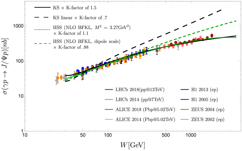
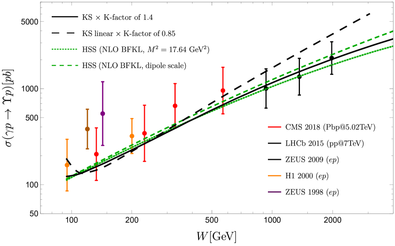
Figure 1: Energy dependence of the $J/\Psi$ and $\Upsilon$ photo-production cross-section as provided by the KS and HSS gluon distribution. The HSS distribution with dipole size scale corresponds to a specific scale setting for the HSS gluon discussed in Sec. 3. For the $J/\Psi$ we further display photo-production data measured at HERA by ZEUS [37, 38] and H1 [39, 40] as well as LHC data obtained from ALICE [41] and LHCb ($W^{+}$ solutions) [42, 43]. For the $\Upsilon$ cross-section we show HERA data measured by H1 [44] and ZEUS [45, 46] and LHC data by LHCb [47] and CMS [48, 49].

2.2 Numerical results using standard implementations

The main uncertainty left is the scale at which the strong coupling constant $\alpha_{s}$ is to be evaluated in Eq. (9). In the case of the $J/\Psi$, which is characterized by a relatively small hard scale $m_{c}\simeq 1.4$ GeV and therefore large value of the strong coupling constant $\alpha_{s}\simeq 0.31$, this leads to a sizable ambiguity in the normalization of the total cross-section, since the latter depends through Eq. (1) quadratically on $\alpha_{s}$. Using similar conventions as used in original fits of the KS and HSS gluon distributions, we fix this scale to a typical hard scale of the process. For the KS gluon we chose both for the photo-production of $\Upsilon$ and $J/\Psi$ vector mesons, the mass of the respective heavy quark as the hard scale; for the HS-gluon it was found in [27] that a scale related to the size of the $J/\Psi$ wave function is more suitable in the case of $J/\Psi$-production, $M_{J/\Psi}^{\text{HS}}=8/\mathcal{R}_{J/\Psi}^{2}=3.27$ GeV while we use the bottom quark mass for $\Upsilon$-production. The results of our study for the fixed scale case can be found in Fig. 1, where continuous, black lines correspond to the KS-gluon and dotted, green lines to the HS-gluon at fixed scales; the dashed green lines, corresponding to a special scale setting of the HSS gluon, and the linear KS-gluon will be discussed in the forthcoming section. We observe that both the KS-gluon distribution and the HSS-gluon distribution provide an excellent description of the energy dependence of the data. While the KS-gluon requires in the current study a K-factor of $1.4-1.5$, we note that the size of such a correction strongly depends on the precise scale choice of the strong coupling constant and the precise parametrization used for the $t$-slope parameter $B_{D}$, Eq. (2). Indeed, using the parametrization of the $B_{D}$ parameter suggested in [18], would bring the K-factor of the KS-gluon close to one in the case of $\Upsilon$-photo-production. We further note that our study does not include a frequently employed phenomenological corrective factor which can be determined through relating the inclusive collinear gluon distribution to generalized parton distribution through a Shuvaev transform. While the precise numerical value of this factor depends on the energy dependent slope parameter $\lambda$, it generally provides a correction which is of the order of the K-factor found for the KS-gluon. Our general conclusion is that the theoretical accuracy of the observable is currently not sufficient to fix unambiguously the normalization. At the same time, the energy dependence is described in an excellent way, both by KS-evolution (non-linear BK evolution combined with DGLAP corrections and kinematical constraint and collinear resummation) and the HSS-gluon (NLO BFKL evolution with collinear resummation).

3 The need for non-linear low $x$ evolution

At first sight it appears that both non-linear $W$ evolution (KS) and linear $W$ evolution (HSS) describe the $W$-dependence of data; one might be therefore lead to conclude that non-linear effects, associated with the presence of high and saturated gluon densities, are absent and the observables merely probes the linear, dilute regime. In the following we argue that such a conclusion is pre-mature. Indeed there are strong hints which suggest that we are at least in the transition region towards high and saturated gluon densities.

To fully access this question, we first recapitulate which possible impact large gluon densities could have on the observable. First of all, the presence of high density effects cannot be seen directly at the level of the observable. The scattering amplitude Eq. (5) depends only on the dipole amplitude, which itself can be expressed as the correlator of two Wilson lines which resum the gluonic field of the proton, see e.g. [50]. Even though the dipole amplitude resums the interaction of the $q\bar{q}$-dipole with an infinite number of gluons, the gluons couple to the $q\bar{q}$-dipole like a single gluon; the “reggeize” in the language of [51] and therefore appear like a single gluon. At the level of our phenomenological study, this property reveals itself through Eq. (9), which relates the dipole cross-section to the unintegrated gluon density. To make multiple re-scattering of partons on the target field visible, it would be necessary to resolve the hadronic final state of the dissociated photon, see e.g. [52, 53]. This not the case for photo-production of vector mesons. The only place where one could expect a signal for the presence of saturation effects is therefore the $x$-dependence of the underlying gluon distributions. As an immediate consequence, any framework which is based on a direct fit of the $x$-dependence at the $J/\Psi$ scale (such as collinear parton distribution functions) does not exclude presence of saturation effects; it merely demonstrates the ability to fit the resulting $x$-dependence of the underlying gluon distribution. While this initial $x$-distribution can be evolved through DGLAP evolution to events with higher hard scales, such events are generally characterized by larger values of $x$ ($x_{\Upsilon}>2.28\cdot 10^{-5}$ vs. $x_{J/\Psi}>2.99\cdot 10^{-6}$ in the current case). Taking further into account that DGLAP evolution is known to shift large $x$ input to lower $x$, it is therefore safe to say that the mere ability of DGLAP fits to accommodate low $x$ $J/\Psi$ photo-production data, does not exclude the potential presence of sizable non-linear effects for the data points at highest $W$-values.

Instead of DGLAP evolution, a suitable benchmark to establish presence/absence of gluon saturation is provided by linear NLO BFKL evolution, such as the HSS gluon. While the HSS gluon provides a very good description of both $\Upsilon$ and $J/\Psi$ photo-production data, the following observation can be made: Recalling the particularly solution of NLO BFKL evolution used for the HSS-fit, one finds at the at level of the dipole cross-section two terms

$$\sigma_{q\bar{q}}^{(\text{HSS})}(x,r) =\alpha_{s}\hat{\sigma}_{q\bar{q}}^{(\text{HSS})}(x,r), \hat{\sigma}_{q\bar{q}}^{(\text{HSS})}(x,r) =\hat{\sigma}_{q\bar{q}}^{(\text{dom.})}(x,r)+\hat{\sigma}_{q\bar{q}}^{(\text{corr.})}(x,r),$$ (10)

where

$$\hat{\sigma}_{q\bar{q}}^{(\text{dom})}(x,r,M^{2}) =\int\limits_{\frac{1}{2}-i\infty}^{\frac{1}{2}+i\infty}\!\!\frac{d\gamma}{2\pi i}\left(\frac{4}{r^{2}Q_{0}^{2}}\right)^{\gamma}\frac{\bar{\alpha}_{s}(M\cdot Q_{0})}{\bar{\alpha}_{s}(M^{2})}f(\gamma,Q_{0},\delta,r)\left(\frac{1}{x}\right)^{\chi\left(\gamma,M^{2}\right)}$$

$$\hat{\sigma}_{q\bar{q}}^{(\text{corr.})}(x,r,M^{2}) =\int\limits_{\frac{1}{2}-i\infty}^{\frac{1}{2}+i\infty}\!\!\frac{d\gamma}{2\pi i}\left(\frac{4}{r^{2}Q_{0}^{2}}\right)^{\gamma}\frac{\bar{\alpha}_{s}(M\cdot Q_{0})}{\bar{\alpha}_{s}(M^{2})}f(\gamma,Q_{0},\delta,r)\left(\frac{1}{x}\right)^{\chi\left(\gamma,M^{2}\right)}$$

$$\times\frac{\bar{\alpha}_{s}^{2}\beta_{0}\chi_{0}\left(\gamma\right)}{8N_{c}}\log{\left(\frac{1}{x}\right)}\Bigg{[}-\psi\left(\delta-\gamma\right)+\log\frac{M^{2}r^{2}}{4}-\frac{1}{1-\gamma}-\psi(2-\gamma)-\psi(\gamma)\Bigg{]}\;,$$ (11)

and

$$f(\gamma,Q_{0},\delta,r) =\frac{r^{2}\cdot\pi\Gamma(\gamma)\Gamma(\delta-\gamma)}{N_{c}(1-\gamma)\Gamma(2-\gamma)\Gamma(\delta)},$$ (12)

is a function which collects both factors resulting from the proton impact factor and the transformation of the unintegrated gluon density to the dipole cross-section, see [28, 27] for details. The parameters $Q_{0}=0.28$ GeV, $\mathcal{C}=2.29$ and $\delta=6.5$ have been determined from the HERA data fit. Furthermore $\bar{\alpha}_{s}=\alpha_{s}N_{c}/\pi$ with $N_{c}$ the number of colors, and $\chi(\gamma,M^{2})$ is the next-to-leading logarithmic (NLL) BFKL kernel after collinear improvements; in addition large terms proportional to the first coefficient of the QCD beta function, $\beta_{0}=11N_{c}/3-2n_{f}/3$ have been resumed through employing a Brodsky-Lepage-Mackenzie (BLM) optimal scale setting scheme [54]. The NLL kernel with collinear improvements reads

$$\chi\left(\gamma,M^{2}\right) ={\bar{\alpha}}_{s}\chi_{0}\left(\gamma\right)+{\bar{\alpha}}_{s}^{2}\tilde{\chi}_{1}\left(\gamma\right)-\frac{1}{2}{\bar{\alpha}}_{s}^{2}\chi_{0}^{\prime}\left(\gamma\right)\chi_{0}\left(\gamma\right)+\chi_{\text{RG}}({\bar{\alpha}}_{s},\gamma,\tilde{a},\tilde{b}).$$ (13)

where $\chi_{i}$, $i=0,1$ denotes the LO and NLO BFKL eigenvalue and $\chi_{\text{RG}}$ resums (anti-)collinear poles to all orders; for details about the individual kernels see [28, 27]. The scale $M$ is a characteristic hard scale of the process. The second contribution $\hat{\sigma}^{\text{corr.}}$ is proportional to $\beta_{0}$ and acts in $\gamma$-space as a differential operator on the impact factors of external particles. These terms do not exponentiate and have been therefore treated in [28] as a perturbative correction to the BFKL Green’s function. Even though $\hat{\sigma}^{\text{corr.}}$ is suppressed by a factor of $\alpha_{s}^{2}$, enhancement by $\ln(1/x)$ will eventually compensate for the smallness of the strong coupling constant and invalidate the perturbative expansion.

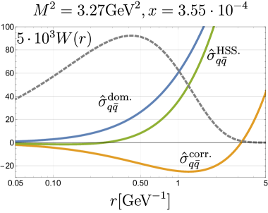
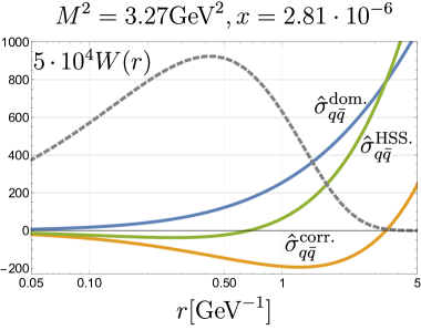
(a)

(b)

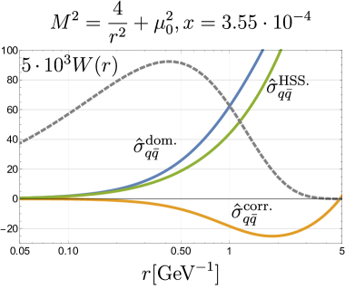
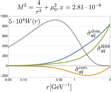
(c)

(d)

Figure 2: HSS dipole cross-section (with an overall factor of $\alpha_{s}$ extracted) at fixed ($J/\Psi$-scale, top row) and $r^{2}$-dependent scale (bottom row) in units of GeV^-2. We also show the function $W(r)$ (times a suitable scaling factor) with which the dipole cross-sections are convoluted with to indicate the typical dipole sized probed in $J/\Psi$ photo-production.

The behavior of the HSS-dipole cross-section is studied in Fig. 2. To identify the relevant region in dipole size $r$ for $J/\Psi$ photo-production we further define

$$W(r) =2\pi r\int_{0}^{1}\!\frac{d{z}}{4\pi}\;(\Psi_{V}^{*}\Psi)_{T}(r,z),$$ (14)

as the $z$-integrated wave function overlap. Working with a fixed hard scale $M^{2}=3.27$ GeV² we find in Fig. 2, that the perturbative expansion is well under control for a typical HERA $x$ value of $x=3.55\cdot 10^{-4}$ (Fig. 2.a). Turning however to the lowest $x$ values probed at the LHC of $x=2.81\cdot 10^{-6}$ (Fig. 2.b) we observe that the correction term is generally large; for certain $r$ values, which are further enhanced through the $r$-dependence of $W(r)$, they even super-seed the dominant term, resulting into a negative dipole cross-section. While the dipole cross-section is not an observable, this clearly indicates a breakdown of the perturbative expansion for dipole sizes where the integrated wave function overlap $W(r)$ has its maximum value. The problem of unnaturally large higher order corrections can be fixed by choosing a hard scale related to the transverse size of the dipole. Following the scale setting used in fits [55] of the IP-sat model [56], we may therefore choose $M^{2}=\frac{4}{r^{2}}+\mu_{0}^{2}$ with $\mu_{0}^{2}=1.51~{}\text{GeV}^{2}$. With this scale, we find that the perturbative expansion indeed stabilizes: both for the HERA (Fig. 2.c) and LHC $x$-values (Fig. 2.d) the perturbative term is well under control. Turning with this choice for the hard scale however to data, we find that this scale setting (green dashed line in Fig. 1) describes very well the energy dependence of $\Upsilon$-photo-production as well as $J/\Psi$ photo-production in the HERA region $W<300$ GeV, but fails to describe $J/\Psi$ production at the LHC ($W>300$ GeV). The resulting growth with energy is too strong and the data are no longer described (Fig. 1, top). We therefore conclude that NLO BFKL evolution can only describe data in the region $W>300$ GeV if one accepts very large perturbative corrections, which super-seed for certain dipole sizes the dominant term and which slow down the growth of the cross-section. If the size of these perturbative corrections is reduced using a suitable hard scale, the growth of the HSS-gluon is too strong and cannot be accomodated by data.

The KS-gluon, which is subject to LO-BK evolution with collinear resummation provides a very good description of $J/\Psi$ data in the region $W>300$ GeV. To answer the question whether this description relies on the presence of non-linear terms in the evolution equation, we compare in addition to a linearized KS gluon (dashed black line in Fig. 1). We find that the growth in $W$ is in that case even stronger than for the HSS gluon with dipole size scale. The ability of the KS gluon to describe data is therefore strongly connected to non-linear evolution effects.

4 Conclusion and Discussion

We conclude that there are strong hints for the presence of the saturation effects in exclusive photo-production of $J/\Psi$ at small $x$. While both linear and non-linear low $x$ QCD evolution can describe the data, the former requires the presence of unnaturally large perturbative corrections. Rendering these corrections small, $\Upsilon$-data, characterized by a hard perturbative scale, are still well described while the growth with energy is too strong for $J/\Psi$ data in the LHC region with $W>300$ GeV. The successful description of data by the KS-gluon directly relies on including non-linear terms in the evolution; with those terms being absent, the description breaks down.

To observed slow-down of the growth with energy is one of the core predictions of gluon saturation. We therefore are convinced that the current study provides substantial evidence for the presence of the saturation effects. We wish to note that a related observation has already been made in [16] on the level of dipole models. The current study substantiates this observation through employing dipole cross-sections which are directly subject to linear and non-linear QCD evolution.

Nevertheless it must be noted that the current study is not without deficits: the description is based on LO wave function and LO BK evolution (although supplemented with collinear resummations). To establish the observation made in this letter it is therefore necessary to search for different observables which probe the low $x$ gluon in a similar kinematic regime and to increase further the theoretical accuracy of the underlying framework. Steps to address the latter are currently undertaken in [57, 58] (evolution equations) and [59, 60, 61, 62] (determination of higher order corrections).

5 Acknowledgments

This work is partly supported by the Polish National Science Centre grant no. DEC-2017/27/B/ST2/01985 and by COST Action CA16201 ”Unraveling new physics at the LHC through the precision frontier”.

References

- [1] F. Gelis, Int. J. Mod. Phys. E 24 (2015) no.10, 1530008 doi:10.1142/S0218301315300088 [arXiv:1508.07974 [hep-ph]].
- [2] F. Gelis, E. Iancu, J. Jalilian-Marian and R. Venugopalan, Ann. Rev. Nucl. Part. Sci. 60 (2010) 463 doi:10.1146/annurev.nucl.010909.083629 [arXiv:1002.0333 [hep-ph]].
- [3] L. V. Gribov, E. M. Levin and M. G. Ryskin, Phys. Rept. 100 (1983) 1. doi:10.1016/0370-1573(83)90022-4
- [4] I. Balitsky, Nucl. Phys. B 463 (1996) 99 doi:10.1016/0550-3213(95)00638-9 [hep-ph/9509348].
- [5] J. Jalilian-Marian, A. Kovner, A. Leonidov and H. Weigert, Nucl. Phys. B 504 (1997) 415 doi:10.1016/S0550-3213(97)00440-9 [hep-ph/9701284].
- [6] J. Jalilian-Marian, A. Kovner, A. Leonidov and H. Weigert, Phys. Rev. D 59 (1998) 014014 doi:10.1103/PhysRevD.59.014014 [hep-ph/9706377].
- [7] Y. V. Kovchegov, Phys. Rev. D 60 (1999) 034008 doi:10.1103/PhysRevD.60.034008 [hep-ph/9901281].
- [8] K. J. Golec-Biernat and M. Wusthoff, Phys. Rev. D 59 (1998) 014017 doi:10.1103/PhysRevD.59.014017 [hep-ph/9807513].
- [9] Y. V. Kovchegov and E. Levin, Camb. Monogr. Part. Phys. Nucl. Phys. Cosmol. 33 (2012) 1. doi:10.1017/CBO9781139022187
- [10] J. L. Albacete and C. Marquet, Phys. Rev. Lett. 105 (2010) 162301 doi:10.1103/PhysRevLett.105.162301 [arXiv:1005.4065 [hep-ph]].
- [11] T. Lappi and H. Mantysaari, Nucl. Phys. A 908 (2013) 51 doi:10.1016/j.nuclphysa.2013.03.017 [arXiv:1209.2853 [hep-ph]].
- [12] J. L. Albacete, G. Giacalone, C. Marquet and M. Matas, Phys. Rev. D 99 (2019) no.1, 014002 doi:10.1103/PhysRevD.99.014002 [arXiv:1805.05711 [hep-ph]].
- [13] J. L. Albacete and C. Marquet, Prog. Part. Nucl. Phys. 76 (2014) 1 doi:10.1016/j.ppnp.2014.01.004 [arXiv:1401.4866 [hep-ph]].
- [14] A. Stasto, S. Y. Wei, B. W. Xiao and F. Yuan, Phys. Lett. B 784 (2018) 301 doi:10.1016/j.physletb.2018.08.011 [arXiv:1805.05712 [hep-ph]].
- [15] A. van Hameren, P. Kotko, K. Kutak and S. Sapeta, arXiv:1903.01361 [hep-ph].
- [16] N. Armesto and A. H. Rezaeian, Phys. Rev. D 90, no. 5, 054003 (2014) [arXiv:1402.4831 [hep-ph]].
- [17] V. P. Goncalves, B. D. Moreira and F. S. Navarra, Phys. Rev. C 90, no. 1, 015203 (2014) [arXiv:1405.6977 [hep-ph]].
- [18] V. P. Goncalves, B. D. Moreira and F. S. Navarra, Phys. Lett. B 742, 172 (2015) [arXiv:1408.1344 [hep-ph]].
- [19] H. Kowalski, L. Motyka and G. Watt, Phys. Rev. D 74, 074016 (2006) [hep-ph/0606272].
- [20] B. E. Cox, J. R. Forshaw and R. Sandapen, JHEP 0906, 034 (2009) [arXiv:0905.0102 [hep-ph]].
- [21] B. Ducloué, T. Lappi and H. Mäntysaari, Phys. Rev. D 94 (2016) no.7, 074031 doi:10.1103/PhysRevD.94.074031 [arXiv:1605.05680 [hep-ph]].
- [22] J. Cepila, J. G. Contreras and M. Matas, Phys. Rev. D 99, no. 5, 051502 (2019) doi:10.1103/PhysRevD.99.051502 [arXiv:1812.02548 [hep-ph]].
- [23] S. P. Jones, A. D. Martin, M. G. Ryskin and T. Teubner, J. Phys. G 41, 055009 (2014) [arXiv:1312.6795 [hep-ph]].
- [24] S. P. Jones, A. D. Martin, M. G. Ryskin and T. Teubner, JHEP 1311, 085 (2013) [arXiv:1307.7099].
- [25] S. P. Jones, A. D. Martin, M. G. Ryskin and T. Teubner, J. Phys. G 44, no. 3, 03LT01 (2017) doi:10.1088/1361-6471/aa56ea [arXiv:1611.03711 [hep-ph]].
- [26] A. Szczurek, A. Cisek and W. Schafer, Acta Phys. Polon. B 48 (2017) 1207 doi:10.5506/APhysPolB.48.1207 [arXiv:1704.00444 [hep-ph]].
- [27] I. Bautista, A. Fernandez Tellez and M. Hentschinski, Phys. Rev. D 94 (2016) no.5, 054002 [arXiv:1607.05203 [hep-ph]].
- [28] M. Hentschinski, A. Sabio Vera and C. Salas, Phys. Rev. Lett. 110 (2013) no.4, 041601 [arXiv:1209.1353 [hep-ph]]; Phys. Rev. D 87 (2013) no.7, 076005 [arXiv:1301.5283 [hep-ph]].
- [29] F. G. Celiberto, D. Gordo Gómez and A. Sabio Vera, Phys. Lett. B 786, 201 (2018) doi:10.1016/j.physletb.2018.09.045 [arXiv:1808.09511 [hep-ph]]; A. D. Bolognino, F. G. Celiberto, D. Y. Ivanov and A. Papa, Eur. Phys. J. C 78, no. 12, 1023 (2018) doi:10.1140/epjc/s10052-018-6493-6 [arXiv:1808.02395 [hep-ph]].
- [30] K. Kutak and S. Sapeta, Phys. Rev. D 86 (2012) 094043 doi:10.1103/PhysRevD.86.094043 [arXiv:1205.5035 [hep-ph]].
- [31] J. Kwiecinski, A. D. Martin and A. M. Stasto, Phys. Rev. D 56 (1997) 3991 doi:10.1103/PhysRevD.56.3991 [hep-ph/9703445].
- [32] S. P. Baranov, Phys. Rev. D 76, 034021 (2007).
- [33] S. J. Brodsky, T. Huang and G. P. Lepage, “The Hadronic Wave Function in Quantum Chromodynamics,” SLAC-PUB-2540.
- [34] J. Nemchik, N. N. Nikolaev and B. G. Zakharov, Phys. Lett. B 341, 228 (1994) [hep-ph/9405355], J. Nemchik, N. N. Nikolaev, E. Predazzi and B. G. Zakharov, Z. Phys. C 75, 71 (1997) [hep-ph/9605231], Z. Phys. C 75, 71 (1997) [hep-ph/9605231].
- [35] M. Braun, Eur. Phys. J. C 16 (2000) 337 doi:10.1007/s100520050026 [hep-ph/0001268].
- [36] G. Chachamis, M. Deàk, M. Hentschinski, G. Rodrigo and A. Sabio Vera, JHEP 1509, 123 (2015) [arXiv:1507.05778 [hep-ph]].
- [37] S. Chekanov et al. [ZEUS Collaboration], Eur. Phys. J. C 24, 345 (2002) [hep-ex/0201043].
- [38] S. Chekanov et al. [ZEUS Collaboration], Nucl. Phys. B 695, 3 (2004) [hep-ex/0404008].
- [39] C. Alexa et al. [H1 Collaboration], Eur. Phys. J. C 73, no. 6, 2466 (2013) [arXiv:1304.5162 [hep-ex]].
- [40] A. Aktas et al. [H1 Collaboration], Eur. Phys. J. C 46, 585 (2006) [hep-ex/0510016].
- [41] B. B. Abelev et al. [ALICE Collaboration], Phys. Rev. Lett. 113, no. 23, 232504 (2014) [arXiv:1406.7819 [nucl-ex]]. S. Acharya et al. [ALICE Collaboration], Eur. Phys. J. C 79, no. 5, 402 (2019) doi:10.1140/epjc/s10052-019-6816-2 [arXiv:1809.03235 [nucl-ex]].
- [42] R. Aaij et al. [LHCb Collaboration], J. Phys. G 40, 045001 (2013) [arXiv:1301.7084 [hep-ex]]; J. Phys. G 41, 055002 (2014) [arXiv:1401.3288 [hep-ex]].
- [43] R. Aaij et al. [LHCb Collaboration], JHEP 1810, 167 (2018) doi:10.1007/JHEP10(2018)167 [arXiv:1806.04079 [hep-ex]].
- [44] C. Adloff et al. [H1 Collaboration], Phys. Lett. B 483, 23 (2000) [hep-ex/0003020].
- [45] J. Breitweg et al. [ZEUS Collaboration], Phys. Lett. B 437 (1998) 432 [hep-ex/9807020].
- [46] S. Chekanov et al. [ZEUS Collaboration], Phys. Lett. B 680, 4 (2009) [arXiv:0903.4205 [hep-ex]].
- [47] R. Aaij et al. [LHCb Collaboration], JHEP 1509, 084 (2015) [arXiv:1505.08139 [hep-ex]].
- [48] CMS Collaboration [CMS Collaboration], “Measurement of exclusive Y photoproduction in pPb collisions at ,” CMS-PAS-FSQ-13-009.
- [49] A. M. Sirunyan et al. [CMS Collaboration], Eur. Phys. J. C 79, no. 3, 277 (2019) doi:10.1140/epjc/s10052-019-6774-8 [arXiv:1809.11080 [hep-ex]].
- [50] H. Weigert, Prog. Part. Nucl. Phys. 55, 461 (2005) doi:10.1016/j.ppnp.2005.01.029 [hep-ph/0501087].
- [51] J. Bartels and M. Wusthoff, Z. Phys. C 66, 157 (1995). doi:10.1007/BF01496591
- [52] A. Ayala, M. Hentschinski, J. Jalilian-Marian and M. E. Tejeda-Yeomans, Phys. Lett. B 761, 229 (2016) doi:10.1016/j.physletb.2016.08.035 [arXiv:1604.08526 [hep-ph]]; Nucl. Phys. B 920, 232 (2017) doi:10.1016/j.nuclphysb.2017.03.028 [arXiv:1701.07143 [hep-ph]];
- [53] P. Kotko, K. Kutak, S. Sapeta, A. M. Stasto and M. Strikman, Eur. Phys. J. C 77, no. 5, 353 (2017) doi:10.1140/epjc/s10052-017-4906-6 [arXiv:1702.03063 [hep-ph]].
- [54] S. J. Brodsky, G. P. Lepage and P. B. Mackenzie, Phys. Rev. D 28 (1983) 228.
- [55] A. H. Rezaeian, M. Siddikov, M. Van de Klundert and R. Venugopalan, Phys. Rev. D 87, no. 3, 034002 (2013) doi:10.1103/PhysRevD.87.034002 [arXiv:1212.2974 [hep-ph]].
- [56] J. Bartels, K. J. Golec-Biernat and H. Kowalski, Phys. Rev. D 66, 014001 (2002) doi:10.1103/PhysRevD.66.014001 [hep-ph/0203258]; H. Kowalski and D. Teaney, Phys. Rev. D 68, 114005 (2003) doi:10.1103/PhysRevD.68.114005 [hep-ph/0304189].
- [57] I. Balitsky and G. A. Chirilli, Phys. Rev. D 88 (2013) 111501 doi:10.1103/PhysRevD.88.111501 [arXiv:1309.7644 [hep-ph]].
- [58] M. Hentschinski, A. Kusina, K. Kutak and M. Serino, Eur. Phys. J. C 78 (2018) no.3, 174 doi:10.1140/epjc/s10052-018-5634-2 [arXiv:1711.04587 [hep-ph]]. M. Hentschinski, A. Kusina and K. Kutak, Phys. Rev. D 94 (2016) no.11, 114013 doi:10.1103/PhysRevD.94.114013 [arXiv:1607.01507 [hep-ph]]. O. Gituliar, M. Hentschinski and K. Kutak, JHEP 1601 (2016) 181 doi:10.1007/JHEP01(2016)181 [arXiv:1511.08439 [hep-ph]].
- [59] M. Hentschinski, Phys. Rev. D 97 (2018) no.11, 114027 doi:10.1103/PhysRevD.97.114027 [arXiv:1802.06755 [hep-ph]]. M. Hentschinski and A. Sabio Vera, Phys. Rev. D 85 (2012) 056006 [arXiv:1110.6741 [hep-ph]]; M. Hentschinski, Nucl. Phys. B 859 (2012) 129 [arXiv:1112.4509 [hep-ph]]; G. Chachamis, M. Hentschinski, J. D. Madrigal Martinez and A. Sabio Vera, Nucl. Phys. B 876 (2013) 453 [arXiv:1307.2591 [hep-ph]]; Phys. Rev. D 87 (2013) no.7, 076009 [arXiv:1212.4992]; Nucl. Phys. B 861 (2012) 133 [arXiv:1202.0649 [hep-ph]]; M. Hentschinski, J. D. Madrigal Martínez, B. Murdaca and A. Sabio Vera, Phys. Lett. B 735 (2014) 168 [arXiv:1404.2937 [hep-ph]]; Nucl. Phys. B 887 (2014) 309 [arXiv:1406.5625 [hep-ph]]; Nucl. Phys. B 889 (2014) 549 [arXiv:1409.6704 [hep-ph]];
- [60] H. Hänninen, T. Lappi and R. Paatelainen, Annals Phys. 393 (2018) 358 doi:10.1016/j.aop.2018.04.015 [arXiv:1711.08207 [hep-ph]].
- [61] I. Balitsky and G. A. Chirilli, Phys. Rev. D 83 (2011) 031502 doi:10.1103/PhysRevD.83.031502 [arXiv:1009.4729 [hep-ph]].
- [62] G. Beuf, Phys. Rev. D 96 (2017) no.7, 074033 doi:10.1103/PhysRevD.96.074033 [arXiv:1708.06557 [hep-ph]]. R. Boussarie, A. V. Grabovsky, D. Y. Ivanov, L. Szymanowski and S. Wallon, Phys. Rev. Lett. 119 (2017) no.7, 072002 doi:10.1103/PhysRevLett.119.072002 [arXiv:1612.08026 [hep-ph]]. R. Boussarie, A. V. Grabovsky, L. Szymanowski and S. Wallon, JHEP 1611 (2016) 149 doi:10.1007/JHEP11(2016)149 [arXiv:1606.00419 [hep-ph]].
- [63] F. D. Aaron et al. [H1 and ZEUS Collaborations], JHEP 1001 (2010) 109 doi:10.1007/JHEP01(2010)109 [arXiv:0911.0884 [hep-ex]].