Induced QCD II: Numerical results

Abstract

We numerically explore an alternative discretization of continuum $\text{SU}(N_{c})$ Yang-Mills theory on a Euclidean spacetime lattice, originally introduced by Budzcies and Zirnbauer for gauge group $\text{U}(N_{c})$. This discretization can be reformulated such that the self-interactions of the gauge field are induced by a path integral over $N_{b}$ auxiliary bosonic fields, which couple linearly to the gauge field. In the first paper of the series we have shown that the theory reproduces continuum $\text{SU}(N_{c})$ Yang-Mills theory in $d=2$ dimensions if $N_{b}$ is larger than $N_{c}-\frac{3}{4}$ and conjectured, following the argument of Budzcies and Zirnbauer, that this remains true for $d>2$. In the present paper, we test this conjecture by performing lattice simulations of the simplest nontrivial case, i.e., gauge group $\text{SU}(2)$ in three dimensions. We show that observables computed in the induced theory, such as the static $q\bar{q}$ potential and the deconfinement transition temperature, agree with the same observables computed from the ordinary plaquette action up to lattice artifacts. We also find that the bound for $N_{b}$ can be relaxed to $N_{c}-\frac{5}{4}$ as conjectured in our earlier paper. Studies of how the new discretization can be used to change the order of integration in the path integral to arrive at dual formulations of QCD are left for future work.

1 Introduction

In the strong-coupling limit of lattice gauge theories, gauge fields do not interact directly with each other, leading to a factorization of the link integrals in the path integral. This allows both for analytical investigations and for the construction of new simulation algorithms (e.g., Blairon:1980pk ; KlubergStern:1981wz ; Kawamoto:1981hw ; Rossi:1984cv ; Karsch:1988zx ). Away from the strong coupling limit the self-interactions of the gauge field need to be taken into account and, with the standard actions, gauge integrals no longer factorize, spoiling the applicability of these strong-coupling methods. A particular way to overcome this problem is to reformulate the gauge action in terms of auxiliary degrees of freedom so that the gauge fields only couple to these unphysical degrees of freedom rather than among themselves (e.g., Bander:1983mg ; Hamber:1983nm ; Kazakov:1992ym ; Hasenfratz:1992jv ). In this approach the gauge action is “induced” in a well-defined limit only after the auxiliary degrees of freedom have been integrated out. Typically this involves taking the limit to an infinite number of fields, rendering the resulting theories impractical for numerical simulations.

In Budczies:2003za , Budczies and Zirnbauer (BZ) developed a method which induces the pure gauge dynamics already for a fixed and small number of auxiliary bosonic fields. The key idea is to give up on the exact reproduction of the Wilson gauge action at finite lattice spacing in favor of an alternative lattice discretization of Yang-Mills theory which allows for a formulation in terms of auxiliary bosons. The vital ingredients for this idea to work are (a) the existence of a continuum limit and (b) its equivalence with continuum Yang-Mills theory. For the “designer action” (or weight factor) introduced in Budczies:2003za , BZ could show these properties for gauge group $\text{U}(N_{c})$ as long as the number of auxiliary bosonic fields, $N_{b}$ is larger or equal to $N_{c}$. In QCD we are interested in gauge group $\text{SU}(N_{c})$ and in Brandt:2016duy (the first paper of this series) we adapted the BZ approach to this case, avoiding a spurious sign problem in the bosonization of the original formulation by a slight reformulation of the original weight factor. In particular, we could show the existence of the continuum limit as long as $N_{b}$ is larger than or equal to $N_{c}-1$ (or $N_{c}-5/4$ if we allow $N_{b}$ to be non-integer) and the equivalence with $\text{SU}(N_{c})$ Yang-Mills theory in the continuum limit. As in the original BZ paper, the latter could be shown in $d=2$ dimensions if $N_{b}\geq N_{c}$ (or $N_{b}\geq N_{c}-3/4$ if we take $N_{b}$ to be non-integer), but it is a conjecture for $d>2$. A brief review of the main findings from Brandt:2016duy which are of importance in this article is included in section 2.

In the present article we will investigate the conjecture numerically for the simplest nontrivial case, namely $\text{SU}(2)$ gauge theory in three dimensions. We simulate both the standard theory with the Wilson plaquette action, which involves a single parameter $\beta$, and the induced theory with a fixed number of bosonic fields $N_{b}$, which involves a single parameter $\alpha$. We set the scale for both theories by computing the Sommer scale $r_{0}$ Sommer:1993ce from the static quark-antiquark potential. Matching $r_{0}$ from both theories gives us a relation between $\alpha$ and $\beta$. Using this relation we can compare other observables, such as quantities connected to the static $q\bar{q}$ potential and the finite-temperature phase transition. We find that the results agree very well already away from the continuum limit and that the agreement improves as the continuum limit is approached. A preliminary analysis of data from $\text{SU}(3)$ gauge theory in four dimensions shows that the modified BZ method also works as expected, supporting the universality argument given in Budczies:2003za . Therefore the modified BZ method, combined with a suitable strong-coupling approach, can be used to reformulate lattice gauge theories in a number of different ways. It will be very interesting to explore such reformulations in the future to see whether they may have advantages over the traditional formulation (and perhaps even solve the sign problem afflicting lattice QCD at nonzero density). We remark that an exact rewriting of the pure gauge action in terms of auxiliary fields has recently been achieved with Hubbard-Stratonovich transformations Vairinhos:2014uxa . This leads to a qualitatively similar reformulation of the theory, even though the auxiliary fields are rather different. These two types of reformulations can thus be seen as complementary approaches with different properties concerning possible reformulations in terms of dual variables.

This paper is structured as follows. In section 2 we review the results from the first paper in the series Brandt:2016duy . The matching between the lattice couplings in Wilson’s pure gauge theory and in the induced gauge theory is discussed in section 3. In sections 4 and 5 we compare the results for the static $q\bar{q}$ potential and the deconfinement phase transition, respectively, before we conclude in section 6. The details concerning the simulation algorithms and the extraction of the observables as well as the details of the simulations for comparison between perturbation theory and numerical results presented in Brandt:2016duy are collected in the appendixes. First reports of our study have been published in Brandt:2014rca ; Brandt:2015nql .

2 Induced pure gauge theory for gauge group $\text{SU}(N_{c})$

We start by reviewing the results from Brandt:2016duy which are relevant for this paper. The weight factor of the alternative discretization of Yang-Mills theory can be written in the form

$$\omega_{\text{IPG}}[U]=\prod_{p}\Big{[}\det\big{(}1-\frac{\alpha}{2}\big{(}U_{p}+U_{p}^{\dagger}\big{)}\big{)}\Big{]}^{-N_{b}},$$ (1)

where we have adopted the notation used in Brandt:2016duy . Here, $0\leq\alpha<1$ is the lattice coupling, the index $p$ labels (unoriented) plaquettes, $U_{p}$ is the product of link variables around the plaquette $p$, and $N_{b}$ is the number of bosonic fields in the bosonized version of the weight factor. The weight factor (1) is a reformulation of the original weight factor introduced in Budczies:2003za so that one obtains a real action after bosonization (cf. section 2.2 in Brandt:2016duy ). Note that in this formulation of the theory $N_{b}$ is just a (positive) number and thus can take any non-integer value, while the bosonization is only possible for integer $N_{b}$. The weight factor is designed in such a way that, for a given value of $N_{b}$ above the bound in eq. (2), the continuum limit is obtained when $\alpha\to 1$.

In Brandt:2016duy we have shown for gauge group $\text{SU}(N_{c})$ that the theory associated with the weight factor (1), which we denote as “induced pure gauge theory” (IPG), approaches a continuum limit for $\alpha\to 1$ as long as

$$N_{b}\geq N_{c}-\frac{5}{4}\,.$$ (2)

Furthermore, in two dimensions the theory in the continuum limit is equivalent to continuum Yang-Mills (YM) theory if

$$N_{b}\geq N_{c}-\frac{3}{4}\,.$$ (3)

For $d>2$ the equivalence is a conjecture based on a universality argument made in Budczies:2003za . As shown in Brandt:2016duy , another way of approaching the continuum limit is to send $N_{b}\to\infty$ while keeping $\alpha$ constant. In particular, the lattice theory becomes equivalent to pure gauge theory with the Wilson plaquette action Wilson:1974sk

$$S_{W}[U]=-\frac{\beta}{N_{c}}\sum_{p}\operatorname{\text{Re}}\operatorname{\text{Tr}}U_{p}$$ (4)

at lattice coupling $\beta$ when sending $\alpha\to 0$ and $N_{b}\to\infty$ while keeping $\beta\sim N_{b}\alpha$ fixed. We will refer to the lattice theory with action (4) as “Wilson pure gauge theory” (WPG). The phase diagram of IPG theory is shown in figure 1 in the parameter space of $N_{b}$ and $\alpha$.

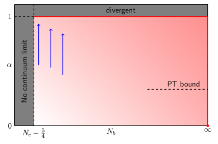
Figure 1: The conjectured phase diagram of $\text{SU}(N_{c})$ induced pure gauge theory in the parameter space of the number of bosons $N_{b}$ and the coupling $\alpha$. The darker shading in red indicates the approach to the continuum theory, indicated by the red lines. The dashed black line in the lower right corner indicates the bound $\alpha=1/3$ below which perturbation theory for $N_{b}\to\infty$ is valid. The blue arrows indicate the interesting region for simulations.

In standard discretizations of Yang-Mills theory one can investigate the nature of the continuum limit by using lattice perturbation theory, making use of the fact that the bare lattice coupling $g$ goes to zero in the continuum limit. As noted in (Brandt:2016duy, , sec. 4.1), such an expansion is not possible in IPG theory around $\alpha=1$ due to the absence of a Gaussian saddle point. An alternative is to expand the theory around the saddle point for fixed $\alpha<1/3$ and $N_{b}\to\infty$ and to analytically continue the results to the region where $\alpha\to 1$. The associated bound for perturbation theory is shown as the black dashed line in figure 1. Using this expansion one finds that a suitable definition of the coupling in IPG theory in the region $\alpha\to 1$ is given by

$$\frac{1}{g_{I}^{2}}=d_{0}(N_{b})\frac{\alpha}{2(1-\alpha)}\,,$$ (5)

where $d_{0}$ is a perturbative coefficient. The relation between the couplings $g_{W}$ and $g_{I}$ in WPG and IPG, respectively, is then given by

$$\frac{1}{g_{W}^{2}}=\frac{1}{g_{I}^{2}}\left(1+d_{1}(N_{b})g_{I}^{2}+\ldots\right)$$ (6)

with another perturbative coefficient $d_{1}$. The formulas for the coefficients are given in (Brandt:2016duy, , eqs. (4.12) and (4.13)).

We remark that the weight factor (1) respects center symmetry, similar to standard Yang-Mills theory and its discretizations. This is due to the fact that the weight factor is formulated in terms of the plaquette $U_{p}$, which itself is a center-symmetric object. Center symmetry is of fundamental relevance for the order of the deconfinement transition, which we will study in section 5.

3 Simulation setup and parameter tuning

We would like to test the conjecture that the continuum limit of IPG reproduces continuum Yang-Mills theory for $d>2$ when the continuum limit exists, i.e., if eq. (2) is fulfilled. To this end, we compare results obtained from IPG and WPG while taking the continuum limit. The first step along the way is to match the bare parameters such that the simulations in IPG and WPG are done at similar lattice spacings $a$. In this section we will discuss the matching for the test case of three-dimensional $\text{SU}(2)$ gauge theory. This is the computationally cheapest non-trivial case to test the conjecture. From the theoretical point of view there is nothing special about this particular case, so that the results obtained here can be expected to be relevant also for other values of $d>2$ and $N_{c}>2$.

3.1 Simulation setup

We consider pure $\text{SU}(2)$ gauge theory discretized on a hypercubic lattice, for which the expectation value of an observable $O$ is given by

$$\left\langle O\right\rangle_{\text{IPG/WPG}}=\frac{1}{Z}\int_{\text{SU}(2)}[dU]\,O[U]\,\omega_{\text{IPG/WPG}}[U]\,.$$ (7)

Here, $Z$ normalizes $\left\langle 1\right\rangle$ to unity, and $\omega[U]$ is the weight factor, which is given in (1) for IPG and by

$$\omega_{\text{WPG}}[U]=\exp\big{\{}-S_{W}[U]\big{\}}$$ (8)

for WPG with the Wilson plaquette action (4). In IPG a simulation point is characterized by two parameters, $N_{b}$ and $\alpha$, while WPG has only one parameter, $\beta$.

For IPG, we are interested in the continuum limit for a fixed small value of $N_{b}$, i.e., we approach the continuum limit along the blue arrows in figure 1. In particular, we will perform the tests for $N_{b}=1$ and 2. These two cases are convenient to test the bounds in eqs. (2) and (3) because both cases satisfy the first bound, which guarantees the existence of a continuum limit, while $N_{b}=1$ violates the second bound, which guarantees equivalence with YM theory in two dimensions. Following the arguments of section 2, we do not expect the latter bound to be relevant for $d>2$.

While WPG can be simulated efficiently with the standard combination of heat-bath Kennedy:1985nu and overrelaxation updates Creutz:1987xi , such algorithms are not available for IPG. We thus use a simple Metropolis algorithm Metropolis:1953am for the simulations, discussed in detail in appendix A.1.

3.2 Scale setting and parameter matching

We set the scale using the Sommer parameter $r_{0}$ Sommer:1993ce . This definition of the lattice scale relies on the physical properties of the static $q\bar{q}$ potential, which can be computed using Polyakov-loop correlation functions, for instance. The details of the extraction of the potential $V(R)$ and the Sommer scale $r_{0}$ are discussed in appendix A.2. Since the change from WPG to IPG amounts to a change of the gauge action only, the operators relevant for the measurement of the potential, together with their spectral representation (cf. appendix A.2) remain unchanged.

We define equivalent lattice spacings by equivalent values of $r_{0}/a$. This means that, for fixed value of $N_{b}$, we match the bare parameters $\beta$ and $\alpha$ so that $\left\langle r_{0}/a\right\rangle_{\text{WPG}}(\beta)=\left\langle r_{0}/a\right\rangle_{\text{IPG}}(\alpha)$. When tuned in such a way, observables are expected to differ by lattice artifacts only, as long as we are close enough to the continuum. Note that the resulting functional dependence $\beta(\alpha)$ is not unique. A similar matching could have been obtained using another observable, such as the string tension $\sigma$, for instance. The resulting matching relations will then differ by lattice artifacts.

The strategy for the matching is the following: We start by fitting the data for $r_{0}$ obtained from simulations of WPG to the expression

$$r_{0}(\beta)=\bar{r}_{0}+\bar{r}_{1}\beta+\bar{r}_{2}\beta^{2}\,.$$ (9)

Performing a simulation of IPG at a fixed value of $\alpha$ and computing the corresponding value of $r_{0}$ then gives us, via inversion of (9), the value of $\beta$ to which this particular $\alpha$ should be matched. This procedure results in a number of pairs $(\alpha,\beta)$ for a given value of $N_{b}$, which we fit to a suitable parameterization $\beta(\alpha)$. The only piece of information we include in this parameterization is the fact that $\beta\to\infty$ should correspond to $\alpha\to 1$. We write the parameterization in the form of an asymptotic series,

$$\beta(\alpha)=\sum_{k=-n}^{K}b_{k}(1-\alpha)^{k}\,.$$ (10)

Perturbation theory supports the validity of such an asymptotic expansion around $\alpha=1$ and suggests $n=1$, see eqs. (5) and (6). However, away from perturbation theory, it is not clear that the asymptotic expansion still provides a good parameterization of $\beta(\alpha)$. This has to be clarified by comparison with the numerical data, and we shall see below that $n=1$ indeed provides the best description, in agreement with perturbation theory.

3.3 Numerical results for the matching

In order to compare the continuum approach of the two theories we have performed simulations at four $\beta$-values for WPG for which high-precision results for the quark-antiquark potential are available Majumdar:2004qx ; HariDass:2007tx ; Brandt:2009tc ; Brandt:2010bw ; Brandt:2013eua ; Brandt:2017yzw ; Brandt:2018fft , i.e., $\beta=5.0$, $7.5$, $10.0$, and $12.5$. For the simulations of IPG we have estimated the interesting range of couplings via the expectation value of the plaquette. We have then chosen three different couplings in this range for $N_{b}=1$ and $N_{b}=2$ to measure Polyakov-loop correlation functions and the Sommer parameter. The simulation parameters are given in table 1. All statistical error bars quoted in the following are Jackknife errors obtained with 100 bins. We have checked explicitly that the error bars and estimates for secondary quantities do not change significantly if we vary the binsize.

Theory	$N_{b}$	coupling		size	$R$	$t_{s}$	$n_{t}$	$\Delta_{\text{sw}}$	meas	$N_{\text{sw}}$	$\epsilon$	$r_{0}$
WPG		$\beta$	5.00	$24^{3}$	2-10	2	5k		2000			3.947(1)(1)
			7.50	$36^{3}$	2-11	2	5k		2000			6.286(7)(1)
			10.00	$48^{3}$	4-19	4	5k		1800			8.603(39)(0)
			12.50	$64^{3}$	4-19	4	5k		1700			10.900(11)(1)
IPG	1	$\alpha$	0.900	$24^{3}$	1-10	2	100k	20	2000	1000	0.14	3.763(1)(2)
			0.930	$36^{3}$	1-11	4	200k	40	2100	1500	0.10	6.161(2)(1)
			0.945	$48^{3}$	1-13	6	500k	100	1700	2000	0.08	8.363(3)(1)
IPG	2	$\alpha$	0.650	$24^{3}$	1-10	2	100k	20	2000	1000	0.14	3.329(1)(1)
			0.750	$36^{3}$	1-11	4	200k	40	2000	1500	0.10	5.969(2)(1)
			0.800	$48^{3}$	1-13	6	500k	100	2000	2000	0.08	8.252(2)(1)

Table 1: Simulation parameters and results for the measurements of $r_{0}$ in pure $\text{SU}(2)$ gauge theory with Wilson action (WPG) and induced action (IPG) for $N_{b}=1$ and 2. Here, $R$ gives the range of $q\bar{q}$ separations used in the analysis of Polyakov-loop correlation functions, $t_{s}$ is the temporal extent of the Lüscher-Weisz sublattices, $n_{t}$ is the number of sublattice updates, $\Delta_{\text{sw}}$ is the number of sweeps separating two sublattice measurements, $N_{\text{sw}}$ is the number of sweeps between two measurements, and $\epsilon$ is the size of the ball for the link proposal. For more details on the algorithms, e.g., the choice of $\Delta_{\text{sw}}$ and $N_{\text{sw}}$, see appendix A.

The methodology for the extraction of $r_{0}$ introduced in appendix A.2 relies on the assumption that IPG is a confining gauge theory for $\alpha<1$. This is not guaranteed, but the existence of a minimal coupling after which the theory is confining in the approach to the continuum limit is a necessary criterion for the approach to continuum Yang-Mills theory. The simulations have shown that this is the case for all couplings of table 1 so that we can extract $r_{0}$ and use it for scale setting. The results for $r_{0}$ are also listed in table 1. The first error is statistical, and the second error is the uncertainty associated with the interpolation. Note that we have kept the volume at $L/r_{0}\gtrsim 7$ in order to ensure that finite size effects for $r_{0}$ are small. That this is indeed the case can be seen from a comparison of the data presented in table 1 and the results for $r_{0}$ given in Brandt:2013eua ; Brandt:2017yzw , where $L/r_{0}\gtrsim 10$. The different results are in very good agreement within the statistical accuracy.

Fit	parameters			$\chi^{2}/$dof
WPG eq. (9)	$\bar{r}_{0}$	$\bar{r}_{1}$	$\bar{r}_{2}$
	-0.79(3)	0.957(9)	-0.0017(6)	0.01
IPG eq. (11)	$b$	$b_{0}$	$n$
$N_{b}=1$	0.54(25)	-1.0(2)	1.00(1)	$\diagup$
$N_{b}=2$	2.51(24)	-2.8(4)	0.99(5)	$\diagup$
IPG eq. (12)	$b_{-1}$	$b_{0}$	$b_{1}$
$N_{b}=1$	0.623(14)	-1.78(11)	3.6(7)	$\diagup$
$N_{b}=2$	2.453(14)	-2.62(12)	-0.1(3)	$\diagup$
IPG eq. (12); $b_{1}=0$	$b_{-1}$	$b_{0}$
$N_{b}=1$	0.602(1)	-1.218(19)		109
$N_{b}=2$	2.463(4)	-2.694(14)		2.2

Table 2: Results for the parameters of the matching fits (see text). If $\chi^{2}/$dof is not given, the parameterizations contain as many parameters as data points.

We start the matching of the two theories by fitting the WPG data to the form given in eq. (9). The results are given in table 2. Note that we have added statistical and systematic uncertainties in quadrature when fitting the data, which likely overestimates the true uncertainties and can thus explain the rather small value of $\chi^{2}/$dof in the fit. Using these results as a definition for the behavior of $r_{0}$ with $\beta$, we then try to find a matching between $\beta$ and $\alpha$ which leads to identical values of $r_{0}$ in the two theories. The guideline for the functional form of $\beta(\alpha)$ is eq. (10). First, it is necessary to determine the leading-order of the divergence of $\beta$ in the limit $\alpha\to 1$. To this end the data for $r_{0}$ obtained in IPG are parameterized by eq. (9) and the parameters from table 2, with $\beta$ replaced by

$$\beta(\alpha)=\frac{b}{(1-\alpha)^{n}}+b_{0}\,,$$ (11)

where $b$, $b_{0}$, and $n$ are free parameters. Note that this is not a fit, since there are as many free parameters as data points. The results for the parameters are listed in table 2. The important information is that in both cases, $N_{b}=1$ and $N_{b}=2$, we have $n\approx 1$ to good accuracy, implying that we can expect the divergence to be a simple pole. This suggests that a suitable parameterization of $\beta(\alpha)$ is given by

$$\beta(\alpha)=\frac{b_{-1}}{1-\alpha}+b_{0}+b_{1}(1-\alpha)+\ldots$$ (12)

We test this parameterization by comparison to the data, using either all three terms (in which case there is no fit) or setting $b_{1}=0$ (in which case we have a fit with one degree of freedom). The resulting parameters are also listed in table 2. We see that the parameters with $b_{1}\neq 0$ and $b_{1}=0$ are in good agreement for $N_{b}=2$ while there are some deviations for $N_{b}=1$. It appears that this is due to the large correction of the term including $b_{1}$, which also leads to a large value of $\chi^{2}/$dof for the fit where $b_{1}=0$ with $N_{b}=1$. Even though a $\chi^{2}/$dof of 2.2 is not satisfactory, the fit for the $N_{b}=2$ case, in contrast, works reasonably well. Since in both cases the correction term including $b_{1}$ is not negligible (for $N_{b}=2$ signaled by $\chi^{2}/\text{dof}>2$) we take the parameterization with $b_{1}\neq 0$ for the matching between $\beta$ and $\alpha$,

$$\beta(\alpha) =\frac{0.623(\phantom{1}4)}{1-\alpha}-1.78(11)+3.6(7)(1-\alpha)\quad\text{for }N_{b}=1\,,$$ (13a)

$$\beta(\alpha) =\frac{2.453(14)}{1-\alpha}-2.62(12)-0.1(3)(1-\alpha)\quad\text{for }N_{b}=2\,.$$ (13b)

This relation will be updated in the next section, see eq. (15) below. Figure 2 shows the data for $r_{0}$ vs $\beta$, including also the data from the induced theory with $\beta$ obtained from (13).

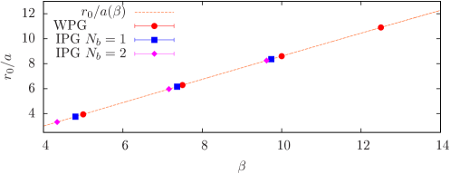
Figure 2: Results for $r_{0}$ vs $\beta$. The $\beta$-values associated with the couplings $\alpha$ for the induced theory have been obtained using (13), which defines the matching $\beta(\alpha)$. The red curve is the interpolating curve (9) with the coefficients from table 2.

The results from this type of matching can also be compared to the results from perturbation theory obtained in Brandt:2016duy . The comparison between the leading-order coefficient $b_{-1}$ to the perturbative coefficient has already been done in section 4.3 of Brandt:2016duy and shows an excellent agreement between numerical data and the perturbative prediction, surprisingly even for $N_{b}=1$. The details of the comparison and the results for larger values of $N_{b}>2$ are summarized in appendix B.

4 The static $q\bar{q}$ potential

After matching the bare couplings of WPG and IPG we are now in a position to compare the results for other observables. In this section we will focus on the static $q\bar{q}$ potential, which is not only important to show that the theory is confining but is also related to an effective string theory for the QCD flux tube (for a recent review see Brandt:2016xsp ). The latter contains non-universal parameters, which can be used to distinguish between different microscopic theories.

4.1 Effective string theory and analysis strategy

A possible way to analyze the static $q\bar{q}$ potential is a comparison to the predictions from the associated effective low-energy theory, namely the effective string theory (EST) for the QCD flux tube, which governs the potential at intermediate and large $q\bar{q}$ separations $R$. The interested reader is referred to the reviews Aharony:2013ipa ; Brandt:2016xsp for further reading about the foundations of the EST and a thorough list of references.

The main result from the EST that we will use in the analysis is the prediction for the $R$ dependence of the static $q\bar{q}$ potential for large $R$ Arvis:1983fp ; Aharony:2010db ; Aharony:2011ga ; Dubovsky:2012sh ; Dubovsky:2014fma ,

$$V^{\text{EST}}(R)=\sigma R\,\sqrt{1-\frac{\pi\>(d-2)}{12\sigma R^{2}}}-\bar{b}_{2}\frac{\pi^{3}(d-2)}{60\sqrt{\sigma^{3}}R^{4}}+\mathcal{O}(R^{-\xi})\,,$$ (14)

where $\sigma$ is the string tension and $\xi=6$ or $\xi=7$, depending on whether the next term in the large-$R$ expansion originates from another boundary term or a bulk term. The first term on the right-hand side is the light-cone (LC) spectrum Arvis:1983fp , which is expected to appear due to the integrability of the leading-order $S$-matrix in the analysis using the thermodynamic Bethe ansatz Dubovsky:2012sh ; Dubovsky:2014fma . The appearance of the full square-root formula is also in good agreement with numerical results for the potential (see Brandt:2016xsp for a compilation of results). The parameter $\bar{b}_{2}$ in eq. (14) is the leading-order boundary coefficient Aharony:2010db ; Aharony:2011ga , which has been found to be non-universal Brandt:2017yzw ; Brandt:2018fft . In the spectrum, possible corrections to the standard EST energy levels, such as the rigidity term, first proposed by Polyakov Polyakov:1996nc , and corrections due to massive modes Dubovsky:2012sh ; Dubovsky:2014fma , have been left out.

Our basic strategy is to try to reproduce, and to compare to, the high-precision results from Brandt:2017yzw , performing the same analysis steps. Since our aim is to perform a like-by-like comparison, rather than validating the string picture, we focus on the basic EST analysis, i.e., sections 3 and 4 in Brandt:2017yzw .

4.2 Simulation points and scale setting

For the comparison we have performed simulations at bare parameters $\alpha$ and volumes that are matched to the parameters in Brandt:2017yzw using the matching relations (13). The new set of parameters is shown in table 3.

Lattice	$N_{b}$	$\alpha$	$\beta^{\text{ref}}$	size	$R$	$t_{s}$	$n_{t}$	$\Delta_{\text{sw}}$	#meas	$N_{\text{sw}}$
I${}^{1}_{1}$	1	0.903	5.00	$48^{3}$	1-10	2	400k	20	2400	2000
I${}^{1}_{2}$	1	0.931	7.50	$64^{3}$	1-15	4	800k	40	2200	3000
I${}^{1}_{3}$	1	0.946	10.0	$96^{3}$	1-22	6	2000k	100	1900	6000
I${}^{2}_{1}$	2	0.680	5.00	$48^{3}$	1-10	2	400k	20	2600	2000
I${}^{2}_{2}$	2	0.759	7.50	$64^{3}$	1-15	4	800k	40	2200	3000
I${}^{2}_{3}$	2	0.806	10.0	$96^{3}$	1-22	6	2000k	100	2000	6000

Table 3: Simulation parameters for the high-precision measurements of the static $q\bar{q}$ potential in simulations with the induced action. $\beta^{\text{ref}}$ is the target value of $\beta$ in WPG theory. The meaning of the other parameters is the same as in table 1. To avoid the propagation of rounding errors, the $\alpha$-values were computed using all digits of $b_{-1}$, $b_{0}$ and $b_{1}$ instead of the rounded values in (13).

For the purpose of scale setting and to check the matching of eq. (13) we have computed the Sommer parameter using the same strategy as before. The results are given in table 4. We can use these results to update the scaling relation (13). For the parameterization with $b_{1}\neq 0$ we obtain

$$\beta(\alpha) =\frac{0.618(\>\>3)}{1-\alpha}-1.63(\>\>9)+2.5(7)(1-\alpha)\quad\text{for }N_{b}=1\,,$$ (15a)

$$\beta(\alpha) =\frac{2.439(15)}{1-\alpha}-2.48(13)-0.5(3)(1-\alpha)\quad\text{for }N_{b}=2\,.$$ (15b)

Lattice	$r_{0}$	$\langle U_{p}\rangle/N_{c}$	$R_{\text{min}}$	$\sqrt{\vphantom{\sigma}\smash{\sigma_{(i)}}}\,r_{0}$	$\sqrt{\vphantom{\sigma}\smash{\sigma_{(ii)}}}\,r_{0}$
I${}^{1}_{1}$	3.9264(5)(39)	0.795094(16)	4	1.2292(17)	1.2309(5)
I${}^{1}_{2}$	6.2804(6)(33)	0.865488(18)	5	1.2398(34)	1.2355(8)
I${}^{1}_{3}$	8.5527(6)(38)	0.898656(15)	8	1.2384(26)	1.2357(6)
I${}^{2}_{1}$	3.9401(3)(44)	0.790699(19)	4	1.2340(28)	1.2320(6)
I${}^{2}_{2}$	6.3121(5)(33)	0.863568(15)	5	1.2342(38)	1.2340(8)
I${}^{2}_{3}$	8.6057(7)(38)	0.898044(14)	8	1.2347(27)	1.2346(7)

Table 4: Results for the Sommer parameter $r_{0}$, the average plaquette $\langle U_{p}\rangle$, the string tension $\sigma$ as obtained from methods (i) and (ii) described in the text, for the simulations listed in table 3.

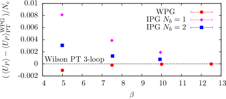
Figure 3: Results for $\langle U_{p}\rangle/N_{c}$ relative to the perturbative result for the Wilson action of eq. (16) vs $\beta$. The $\beta$-values associated with the couplings $\alpha$ for the induced theory have been obtained using eq. (15).

For a first comparison of observables in the approach to the continuum we can look at the expectation value of the plaquette. Even though trivial in the continuum limit, its dependence on the lattice spacing, i.e., the bare coupling, is non-trivial and can be computed in lattice perturbation theory. The three-loop result for $\text{SU}(2)$ WPG in $d=3$ is given by Panagopoulos:2006ky

$$\langle U_{p}\rangle^{\text{WPG}}_{\text{PT}}/N_{c}=1-0.25g_{0}^{2}-0.01453916(4)g_{0}^{4}-0.0053459(2)g_{0}^{6}\,.$$ (16)

The numerical results for the plaquette are listed in table 4 and shown in figure 3. To make the small differences visible we do not display the raw data but rather the difference between the plaquette expectation values and the perturbative result.

The plot shows that the WPG results are already very close to the perturbative result, i.e., lattice artifacts with respect to 3-loop perturbation theory for Wilson’s gauge action are small. From the plot one might be led to the conclusion that lattice artifacts for IPG are larger. However, the coefficients of the perturbative result which we subtracted have been obtained from Wilson’s plaquette action and are expected to be different for IPG in general, and for different values of $N_{b}$ in particular. Indeed, corrections to eq. (16) in WPG theory start at order $g_{0}^{8}$, while for IPG theory corrections start at lower orders.

Another option to set the scale is via the string tension $\sigma$, which governs the linear rise with $R$ of the potential for $R\to\infty$. As in Brandt:2017yzw we extract $\sigma$ with two different methods:

1. We fit the force to the form

   $$R^{2}F(R)=\sigma R^{2}+\gamma\,,$$ (17)

   motivated by the expansion of the EST potential to next-to-leading-order in $1/R$.

2. We fit the potential to

   $$V(R)=\sigma R\,\sqrt{1-\frac{\pi(d-2)}{12\sigma R^{2}}}+V_{0}\,,$$ (18)

   corresponding to the (full) leading-order EST prediction with an additive normalization constant $V_{0}$.

This particular combination of ansätze is especially useful since corrections with respect to the full EST prediction, eq. (14), appear at different orders in the $1/R$ expansion. Consequently, we can determine the region where higher-order terms in the EST are negligible by comparing the results for $\sigma$ from methods (i) and (ii). The basic strategy is to investigate the dependence of $\sigma$ on the minimal value of $R$ included in the fit, $R_{\text{min}}$. In particular, in the region where the results from the two methods agree within errors and show a plateau, higher-order terms are expected to be negligible, and we can use any of the results for $\sigma$.

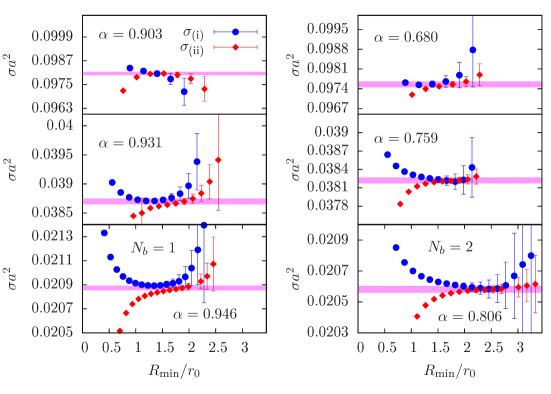
Figure 4: Results for the string tension in IPG for $N_{b}=1$ (left) and $N_{b}=2$ (right) extracted from method (i), $\sigma_{\text{(i)}}$, and (ii), $\sigma_{\text{(ii)}}$, as explained in the text, vs the minimal value of $R$ included in the fit, $R_{\text{min}}$ in units of $r_{0}$. The red bands are the values of $\sigma_{\text{(ii)}}$ which we use for the further analysis.

In figure 4 we show the results for the extraction of the string tension in IPG for $N_{b}=1$ (left) and $N_{b}=2$ (right). We see that for $N_{b}=1$ and $\alpha=0.931$ and 0.946 the results from method (i) already start to leave the plateau region when the results from method (ii) reach the plateau. Nevertheless, the plateau values agree within uncertainties, as the results from method (i) agree within errors at the point where the results from method (ii) reach the plateau region. As the final results for the string tension, we will use the result from method (ii) obtained with the value of $R_{\text{min}}$ where the results of the two methods become consistent. In the cases without a common plateau we use the value of $R_{\text{min}}$ where the result from method (ii) starts to agree with the plateau from method (i). The final results are indicated by the red bands in figure 4. The results for $\sigma$ are listed in table 4. The quoted uncertainties for $\sigma$ include the systematic uncertainties for $r_{0}$, which have been conservatively added in quadrature to the statistical uncertainties.

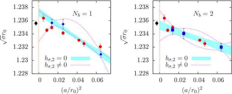
Figure 5: Continuum extrapolations of $\sqrt{\vphantom{\sigma}\smash{\sigma_{(ii)}}}r_{0}$ from IPG for $N_{b}=1$ (left) and $N_{b}=2$ (right). For comparison we also show the results for $\text{SU}(2)$ WPG from Brandt:2017yzw (red circles) and the associated continuum-extrapolated value (black circle).

To compare the results for $\sigma$ with the results for WPG with gauge group $\text{SU}(2)$ from Brandt:2017yzw we show the two sets of results in figure 5 for $N_{b}=1$ (left) and $N_{b}=2$ (right). For $N_{b}=2$ we observe good agreement between the results from IPG and WPG, while some slight differences are visible for $N_{b}=1$. The latter could either be fluctuations, remnants of uncontrolled systematic uncertainties connected to the extraction of $\sigma$, or simply due to the different lattice artifacts in the two theories. Eventually, we expect the results to agree in the continuum limit. To test this, we have performed a continuum extrapolation of the form

$$\sqrt{\sigma}r_{0}=\big{(}\sqrt{\sigma}r_{0}\big{)}^{\text{cont}}+b_{\sigma,1}\Big{(}\frac{a}{r_{0}}\Big{)}^{2}+b_{\sigma,2}\Big{(}\frac{a}{r_{0}}\Big{)}^{4}\,.$$ (19)

As in Brandt:2017yzw we perform two fits, either with $b_{\sigma,2}\neq 0$ or with $b_{\sigma,2}=0$. The resulting extrapolations are also shown in figure 5 together with the extrapolation for WPG from Brandt:2017yzw (black circle). We see that for $N_{b}=2$ the continuum extrapolations are all in very good agreement with the WPG result, even though less precise, which can be expected since only three points are available for the extrapolation. For $N_{b}=1$ the extrapolation linear in $a^{2}$ overshoots the WPG result. However, the data also indicate the importance of higher-order terms. Including the $a^{4}$ term leads to an extrapolation which is fully consistent with the WPG result, albeit with large uncertainties. For comparisons we will use the results from the continuum extrapolation with $b_{\sigma,2}\neq 0$. This extrapolation has larger errors, but the central value agrees well with the continuum-extrapolated WPG result in both cases.

4.3 Results for the static potential

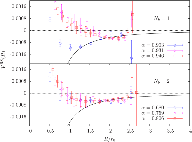
Figure 6: Results for the static potential in its rescaled form, see eq. (20), for different lattice spacings vs $R$ for SU(2) IPG with $N_{b}=1$ (top) and $N_{b}=2$ (bottom). The black continuous line is the light-cone potential obtained with the continuum-extrapolated string tension.

We will now look at the results for the static potential itself. The results for the potential, rescaled according to

$$V^{\text{RS}}(R)=\Big{(}\frac{V(R)-V_{0}}{\sqrt{\sigma}}-R\sqrt{\sigma}\Big{)}\frac{R\sqrt{\sigma}}{\pi}+\frac{1}{24}\,,$$ (20)

are shown in figure 6. As in Brandt:2017yzw the results for the individual couplings have been rescaled using the string tension for this value of $\alpha$, while the solid line is the rescaled version of the leading-order EST prediction, the LC spectrum, with the continuum limit of the string tension.

Results for the static potential in WPG were already presented in figure 3 of Ref. Brandt:2017yzw . We do not reproduce that figure here. The comparison with figure 6 shows one of the main problems we are facing, namely the reduced accuracy of the present study, which is mainly due to the less efficient algorithm for IPG compared to the heat-bath algorithm used in the WPG simulations. This leads to a reduction in the range of $R$ and reduces the precision in the extraction of $\sigma$. Concerning the results for the potential itself, the agreement with the WPG results in (Brandt:2017yzw, , fig. 3) is eminent for $N_{b}=2$ and also visible for $N_{b}=1$, although the lattice with $\alpha=0.903$ appears to be outside the scaling region. As in WPG, the corrections to the LC potential in IPG are positive and tend to become stronger when approaching the continuum limit.

The next step in the analysis is to check whether the leading-order correction to the square-root formula in eq. (14) is indeed of order $R^{-4}$. To this end we fit the data to the form

$$V(R)=\sigma R\,\sqrt{1-\frac{\pi(d-2)}{12\sigma R^{2}}}+\frac{\eta\sqrt{\sigma}}{\big{(}\sqrt{\sigma}R\big{)}^{m}}+V_{0}\,,$$ (21)

where $\eta$, $m$, $\sigma$ and $V_{0}$ are fit parameters. If the predictions of the EST are correct, we will obtain $m=4$. Otherwise we will find $m<4$ if the square-root formula in eq. (21) is incorrect, or $m>4$ if the corrections start at higher order. We show the results for $m$ vs $R_{\text{min}}$ in figure 7. As in $\text{SU}(2)$ WPG, cf. (Brandt:2017yzw, , fig. 4), we typically observe a plateau around $0.5\lesssim R/r_{0}\lesssim 1.0$. For $N_{b}=1$ the uncertainties are typically larger for larger $R$-values, so that the plateau does not last as long as for $N_{b}=2$. The plateau value is typically around $m=3.6$. This slight discrepancy with expectations has also been found in WPG Brandt:2017yzw and indicates a possible mixing with other correction terms. At finite $N_{c}$ the EST will receive corrections from virtual glueball exchange, for instance.

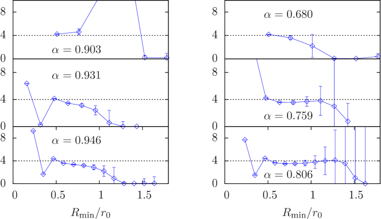
Figure 7: Results for the exponent $m$ plotted vs the minimal value of $R$ included in the fit, $R_{\text{min}}$, for $\text{SU}(2)$ IPG with $N_{b}=1$ (left) and $N_{b}=2$ (right). The horizontal line indicates the exponent of the leading correction to the EST.

4.4 Extraction of the boundary coefficient

To make the comparison of the subleading properties of the potential more quantitative, we will now extract the boundary coefficient $\bar{b}_{2}$. As in Brandt:2017yzw , we include higher-order terms in the fit formula and fit the potential to the form

$$V(R)=V^{\text{EST}}(R)+\frac{\gamma^{(1)}_{0}}{\sqrt{\sigma^{5}}R^{6}}+\frac{\gamma^{(2)}_{0}}{\sigma^{3}R^{7}}+V_{0}\,.$$ (22)

Specifically, we perform the following fits Brandt:2017yzw :

1. We use $\sigma$ and $V_{0}$ from method (ii) as input and fit with $\bar{b}_{2}$, $\gamma^{(1)}_{0}$ and $\gamma^{(2)}_{0}$ as free parameters.

2. We use $\sigma$, $V_{0}$ and $\bar{b}_{2}$ as free parameters and set $\gamma^{(1)}_{0}=0$ and $\gamma^{(2)}_{0}=0$.

3. We use $\sigma$, $V_{0}$, $\bar{b}_{2}$ and $\gamma^{(1)}_{0}$ as free parameters and set $\gamma^{(2)}_{0}=0$.

4. We use $\sigma$, $V_{0}$, $\bar{b}_{2}$ and $\gamma^{(2)}_{0}$ as free parameters and set $\gamma^{(1)}_{0}=0$.

5. We use $\sigma$, $V_{0}$, $\gamma^{(1)}_{0}$ and $\gamma^{(2)}_{0}$ as free parameters and set $\bar{b}_{2}=0$.

The fits are performed for several values of $R_{\text{min}}$, and we extract the final result from the second smallest $R_{\text{min}}$ which provides a $\chi^{2}/\text{dof}<1.5$. The quality of the agreement with the data is then indicated by the value of $R_{\text{min}}$ (smaller values mean better agreement) in context with the number of higher-order terms included in the fit. Fit C, for instance, should allow for a smaller value of $R_{\text{min}}$ compared to fit B since the latter does not contain higher-order correction terms. To check for the systematic uncertainty associated with the fit interval we compare the result to the ones obtained with $R_{\text{min}}\pm a$.

Fit	$\sqrt{\sigma}r_{0}$	$aV_{0}$	$\bar{b}_{2}\cdot 10^{2}$	$\gamma^{(1)}_{0}\cdot 10^{3}$	$\gamma^{(2)}_{0}\cdot 10^{3}$	$\chi^{2}/$dof	$R_{\text{min}}/r_{0}$
$\alpha=0.903$
A	—	—	1.76(20)(235)	43(4)(79)	-27(4)(75)	0.44	0.76
B	1.2317(3)(5)	0.2060(3)( 5)	-1.73(4)(21)	—	—	0.59	0.76
C	1.2314(5)(9)	0.2064(6)(13)	-1.13(55)(449)	2(2)(28)	—	0.61	0.76
D	1.2314(5)(9)	0.2064(6)(12)	-1.30(41)(323)	—	1(2)(23)	0.61	0.76
E	1.2313(4)(6)	0.2066(5)(8)	—	20(10)(54)	-12(12)(62)	0.56	0.76
$\alpha=0.931$
A	—	—	-4.61(194)(49)	-20(18)(7)	10(10)(5)	0.65	0.64
B	1.2347(3)(4)	0.1699(2)(3)	-2.46(10)(42)	—	—	0.47	0.96
C	1.2349(3)(4)	0.1697(2)(3)	-3.27(32)(128)	4(2)(8)	—	0.37	0.80
D	1.2349(3)(3)	0.1697(2)(3)	-2.95(23)(95)	—	3(1)(6)	0.38	0.80
E	1.2348(4)(5)	0.1698(3)(4)	—	73(71)(79)	-65(62)(99)	0.41	0.96
$\alpha=0.946$
A	—	—	-3.56(114)(23)	-9(9)(4)	4(5)(3)	1.06	0.58
B	1.2352(2)(3)	0.1436(1)(2)	-2.48(7)(25)	—	—	0.47	0.94
C	1.2352(2)(4)	0.1436(1)(2)	-2.88(10)(44)	-2(1)(1)	—	0.39	0.70
D	1.2352(2)(4)	0.1436(1)(2)	-2.65(7)(36)	—	-2(1)(2)	0.45	0.70
E	1.2352(3)(3)	0.1436(1)(2)	—	61(61)(32)	-51(51)(38)	0.36	0.94

Table 5: Results of the fits for the extraction of $\bar{b}_{2}$ for $N_{b}=1$ IPG.

Fit	$\sqrt{\sigma}r_{0}$	$aV_{0}$	$\bar{b}_{2}\cdot 10^{2}$	$\gamma^{(1)}_{0}\cdot 10^{3}$	$\gamma^{(2)}_{0}\cdot 10^{3}$	$\chi^{2}/$dof	$R_{\text{min}}/r_{0}$
$\alpha=0.680$
A	—	—	-4.57(460)(288)	-31(58)(93)	18(37)(88)	0.38	0.76
B	1.2317(2)(5)	0.2114(2)(5)	-1.73(3)(17)	—	—	0.29	0.76
C	1.2320(4)(4)	0.2111(4)(6)	-2.17(39)(183)	-2(2)(12)	—	0.25	0.76
D	1.2320(4)(4)	0.2111(4)(5)	-2.05( 30)(134)	—	-1(1)(10)	0.25	0.76
E	1.2317(3)(7)	0.2115(4)(8)	—	29(29)(45)	-20(20)(52)	0.34	0.76
$\alpha=0.759$
A	—	—	-0.11(252)(119)	34(30)(34)	-24(18)(30)	0.26	0.79
B	1.2342(3)(2)	0.1723(2)(2)	-2.25(10)(16)	—	—	0.18	0.95
C	1.2343(3)(1)	0.1722(2)(1)	-2.65(30)(22)	-2(1)(1)	—	0.17	0.79
D	1.2343(3)(2)	0.1722(2)(1)	-2.50(22)(20)	—	-2(1)(1)	0.17	0.79
E	1.2339(3)(5)	0.1726(2)(4)	—	34(34)(13)	-24(24)(14)	0.34	0.76
$\alpha=0.806$
A	—	—	-1.16(267)( 99)	15(28)(21)	-10(16)(16)	0.50	0.70
B	1.2346(2)(3)	0.1445(1)(2)	-2.21(4)(15)	—	—	0.19	0.81
C	1.2349(2)(3)	0.1443(1)(2)	-2.67(12)(32)	-2(1)(1)	—	0.02	0.70
D	1.2348(2)(3)	0.1444(1)(2)	-2.50(9)(26)	—	-1.1(2)(7)	0.03	0.70
E	1.2345(3)(4)	0.1446(1)(2)	—	57(37)(101)	-26(26)(11)	0.08	0.81

Table 6: Results of the fits for the extraction of $\bar{b}_{2}$ for $N_{b}=2$ IPG.

We list the results of the different fits for $N_{b}=1$ and 2 in tables 5 and 6, respectively. Comparing the results to those of (Brandt:2017yzw, , tab. 5), in particular for $\beta=5.0$, 7.5 and 10.0, we see that both the possible fit ranges and the resulting parameters are very similar. The only exception is fit A, for which $\sigma$ and $V_{0}$ have been taken over from section 4.2. Since the extraction of $\sigma$ and $V_{0}$ was not as accurate as in Brandt:2017yzw it is reasonable that this is the main reason for deviations in this particular fit. We can thus follow the discussion of Brandt:2017yzw and conclude that fits B, C and D can be used in the following analysis. Fit E typically requires larger values for $R_{\text{min}}$ compared to fits C and D, even though it also includes two higher-order terms. Thus we conclude that the agreement with the data is worse for fit E than for the other fits. In any case, fit E only serves as a check that, given the data, $\bar{b}_{2}$ does not vanish. Compared to Brandt:2017yzw , where fit E clearly showed less agreement with the data, direct conclusions are more difficult here since the IPG data are less precise than those of WPG.

As in Brandt:2017yzw , we determine the final results for $\bar{b}_{2}$ on the individual lattice spacings via the weighted average over the results from fits B to D, where the weight is given by the uncertainties. To estimate the systematic uncertainty due to the choice of $R_{\text{min}}$ we repeat the procedure with $R_{\text{min}}\pm a$ and use the maximal deviation. The results are tabulated in table 7. Comparing once more to the $\text{SU}(2)$ results of Brandt:2017yzw , which we list for comparison in table 7 as well, we see that the results are similar in magnitude and have similar uncertainties. This is particularly true for $N_{b}=2$. For $N_{b}=1$ the systematic uncertainties are somewhat larger, but the overall agreement is still good. We show the results for $\bar{b}_{2}$ in comparison to the results of Brandt:2017yzw in figure 8. One can clearly see the similar behavior in the approach to the continuum and the good agreement between the results from the different simulations. In particular, the results are significantly different from the ones for $\text{SU}(3)$ gauge theory, showing the discriminating power of the results.

WPG		IPG $N_{b}=1$		IPG $N_{b}=2$
$\beta$	$\bar{b}_{2}$	$\alpha$	$\bar{b}_{2}$	$\alpha$	$\bar{b}_{2}$
5.0	-0.0179( 5)(50)(23)	0.903	-0.0173( 4)(59)(24)	0.680	-0.0174( 4)(43)(19)
7.5	-0.0244(11)(25)(16)	0.931	-0.0260(14)(68)(54)	0.759	-0.0237(16)(28)(14)
10.0	-0.0251( 5)(27)(22)	0.946	-0.0260( 7)(29)(31)	0.806	-0.0233( 6)(35)(19)

Table 7: Final results for $\bar{b}_{2}$ in WPG Brandt:2017yzw and IPG with $N_{b}=1$ and 2 for the individual couplings. The first error is the statistical uncertainty, the second the systematic one due to the unknown higher-order correction terms, estimated by computing the maximal deviations of the results from fits B to D, and the third is the systematic one associated with the choice of $R_{\text{min}}$.

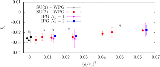
Figure 8: Results for $\bar{b}_{2}$ from table 7 and for $\text{SU}(2)$ WPG from Brandt:2017yzw vs the squared lattice spacing in units of $r_{0}$. Also shown are the continuum results from eq. (24) and the $\text{SU}(2)$ result from (Brandt:2017yzw, , eq. (6.2)). The results for $\text{SU}(2)$ WPG and for $N_{b}=2$ have been slightly shifted to the left and to the right, respectively, to enable the visibility of the different sets of points.

4.5 Continuum limit

Finally, we perform the continuum extrapolation of the boundary coefficient $\bar{b}_{2}$. To this end we parameterize it as Brandt:2017yzw

$$\bar{b}_{2}=\big{(}\bar{b}_{2}\big{)}^{\text{cont}}+b_{\bar{b}_{2},1}\Big{(}\frac{a}{r_{0}}\Big{)}^{2}+b_{\bar{b}_{2},2}\Big{(}\frac{a}{r_{0}}\Big{)}^{4}$$ (23)

and perform two different types of fits:

1. We fit including all terms in eq. (23).

2. We fit with setting $b_{\bar{b}_{2},2}=0$.

Note that fit (1) is a parameterization of the results rather than a fit. In Brandt:2017yzw a third fit has been performed, which included only the data for the finest lattice spacings. Such a fit does not make sense here due to the limited number of available couplings. To estimate the propagation of systematic uncertainties we follow the strategy of Brandt:2017yzw and perform the fits (1) and (2) for the results from fits B to D and the fits with a minimal $R$-value of $R_{\text{min}}\pm a$ individually. The final results have been extracted using a weighted average of the results from fits B to D, once more with the individual uncertainties as weights. As before, the individual systematic uncertainties are computed from the maximal deviations to the different fits. The curves for fit (2) with the main value of $R_{\text{min}}$ are shown in figure 9.

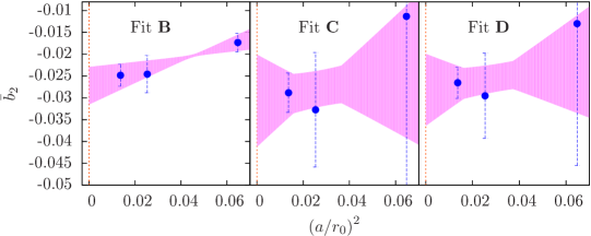
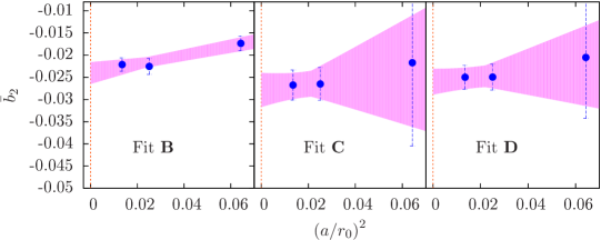
Figure 9: Results for the linear continuum extrapolation, fit (2), for the results for $\bar{b}_{2}$ obtained from fits B, C and D (from left to right) for $\text{SU}(2)$ IPG with $N_{b}=1$ (top) and $N_{b}=2$ (bottom).

$N_{b}$	Fit	(1)	(2)
1	$\big{(}\bar{b}_{2}\big{)}^{\text{cont}}$	-0.0223(37)(40)(44)	-0.0276( 9)(31)(47)
2	$\big{(}\bar{b}_{2}\big{)}^{\text{cont}}$	-0.0214(26)(50)(29)	-0.0244( 6)(34)(24)

Table 8: Results for $\big{(}\bar{b}_{2}\big{)}^{\text{cont}}$ from fits (1) and (2) (see text). The first error is the statistical uncertainty, the second the one associated with the unknown higher-order correction terms in the potential and the third the one due to the choice of $R_{\text{min}}$.

The continuum results for $\bar{b}_{2}$ from fits (1) and (2) are given in table 8. We use the results from fit (1) to estimate the systematic uncertainty associated with the continuum limit. The final results, which we take from fit (2), are thus given by

$$\big{(}\bar{b}_{2}\big{)}^{\text{cont}}=\left\{\begin{array}[]{ll}-0.0276(9)(31)(47)(53)&\quad\text{for}\>\>N_{b}=1\,,\\[5.69054pt] -0.0244(6)(34)(24)(30)&\quad\text{for}\>\>N_{b}=2\,.\end{array}\right.$$ (24)

Those can be compared to the final continuum estimate for $\text{SU}(2)$ WPG from Brandt:2017yzw ,

$$\big{(}\bar{b}_{2}\big{)}^{\text{cont}}=-0.0257\,(3)(38)(17)(3)\,.$$ (25)

In eqs. (24) and (25) the first error is purely statistical, the second is the systematic uncertainty due to the unknown higher-order terms in the potential, the third is the one associated with the particular choice for $R_{\text{min}}$ and the fourth is the systematic uncertainty due to the continuum extrapolation. We see that the results from eqs. (24) and (25) agree well within uncertainties. In addition, the sizes of the individual uncertainties are similar, except for the continuum extrapolation, which, however, is expected since in the IPG analysis ensembles at fewer lattice spacings are available.

We briefly summarize the findings of this section. We have repeated the analysis of the potential in Brandt:2017yzw for IPG and found that in every individual step the results agree extremely well with WPG, for both $N_{b}=1$ and $2$. The whole analysis indicates that the fine structure of the potential in the continuum is indeed identical in IPG and WPG. Hence we can conclude that, at least for the potential, both theories lead to the same continuum limit (up to the accuracy of this study). This is also reflected in the significant difference to the results for $\text{SU}(3)$ WPG, which shows the discriminating power of this comparison.

5 The finite-temperature phase transition

So far we have compared properties of IPG and WPG for observables at vanishing temperature and found good agreement. We will now show that the agreement prevails for thermodynamic observables. In particular, we will consider the deconfinement transition temperature $T_{c}$ and the ratio of critical exponents $\gamma/\nu$. The latter can be regarded as a measure of the universality class of the transition (we expect a phase transition of 2nd order). The fundamental lattice observable that can be used to investigate the deconfinement transition is the absolute value of the Polyakov loop, $\left\langle|L|\right\rangle$, the order parameter associated with the breaking of center symmetry. In particular, we choose a setup which is similar to that in Engels:1996dz so that we can directly compare to this study.

5.1 Simulation parameters and results for the Polyakov loop

Theory	$N_{t}$	volumes	couplings	# meas	$N_{\text{sw}}$
WPG	4	$32^{2}$, $48^{2}$, $64^{2}$, $96^{2}$	5.00-7.50	100k	$\diagup$
IPG $N_{b}=1$	4	$32^{2}$, $48^{2}$, $64^{2}$, $96^{2}$	0.900-0.945	100k-400k	100
IPG $N_{b}=2$	4	$32^{2}$, $48^{2}$, $64^{2}$, $96^{2}$	0.650-0.830	100k-200k	100
WPG	6	$48^{2}$, $72^{2}$, $96^{2}$, $144^{2}$	8.00-11.50	100k	$\diagup$
IPG $N_{b}=1$	6	$48^{2}$, $72^{2}$, $96^{2}$, $144^{2}$	0.930-0.950	400k	100
IPG $N_{b}=2$	6	$48^{2}$, $72^{2}$, $96^{2}$, $144^{2}$	0.750-0.850	$\sim$400k	100

Table 9: Simulation parameters of the finite-temperature runs in 3d $\text{SU}(2)$ IPG and WPG theories. For each volume the simulations have been done on the same values of the coupling. For WPG and $N_{t}=4$ the distance between two $\beta$-values was taken to be $0.01$ in the region around $T_{c}(\infty)$, while for $N_{t}=6$ we used a distance of $0.05$. For IPG theory with $N_{b}=1$, the distance between two $\alpha$-values was taken to be $0.0001$ for $N_{t}=4$ and $0.00025$ for $N_{t}=6$, while for $N_{b}=2$ we used $0.001$ for both $N_{t}=4$ and 6. Away from $T_{c}(\infty)$ we have simulated less frequently. For $N_{t}=4$ the number of measurements varies between the different volumes, and around $T_{c}(\infty)$ we have increased the number of measurements with the volume.

As before, we perform simulations in IPG using $N_{b}=1$ and 2. In addition, we also simulate in WPG for a direct comparison of the results. To test the approach to the continuum limit we use two different temporal extents, $N_{t}=4$ and 6, for which we vary the temperature $T=1/(aN_{t})$ by varying the lattice spacing $a$ via the lattice couplings $\alpha$ and $\beta$. For scale setting we use the results of section 3. The resulting simulation parameters are listed in table 9. For $N_{t}=6$ the volumes have been chosen to match the volumes for $N_{t}=4$ in physical units.

The main observables are the absolute value of the Polyakov loop

$$|L|=\frac{1}{V}\sum_{\vec{x}}\Big{|}\operatorname{\text{Tr}}\prod_{n_{0}=1}^{N_{t}}U_{0}(n_{0}\,a,\vec{x})\Big{|}$$ (26)

and its susceptibility

$$\chi_{L}=V\left(\left<|L|^{2}\right>-\left<|L|\right>^{2}\right).$$ (27)

For each simulation point we have performed at least 100,000 measurements and increased the number of measurements to about 400,000 in the vicinity of $T_{c}$, where the autocorrelations increase due to the approach of a second-order critical point.

The results for $\left\langle|L|\right\rangle$ and $\chi_{L}$ vs the temperature in units of the Sommer parameter are shown in figures 10 and 11 for $N_{t}=4$ and 6, respectively. We always show the two extremal cases of smallest and largest available volume. The plots show the remarkable agreement between the results of WPG and IPG with $N_{b}=1$ and 2. This already indicates the similarity between the corresponding phase transitions. In particular, the volume scaling is equivalent in the different cases so that the universality classes can be expected to be equivalent as well. In the following we will investigate this expectation more quantitatively.

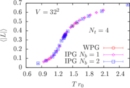
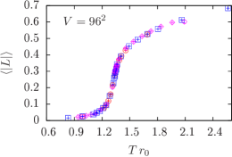
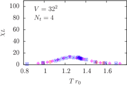
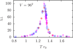
Figure 10: Results for the absolute value of the Polyakov loop $\left\langle|L|\right\rangle$ (top) and its susceptibility $\chi_{L}$ (bottom) at $N_{t}=4$ with volumes $32^{2}$ (left) and $96^{2}$ (right). The legend is the same for all plots.

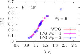
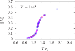
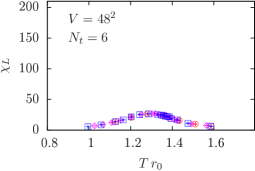
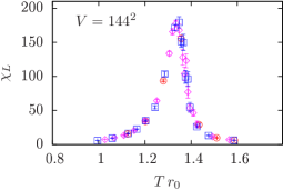
Figure 11: Results for the absolute value of the Polyakov loop $\left\langle|L|\right\rangle$ (top) and its susceptibility $\chi_{L}$ (bottom) at $N_{t}=6$ with volumes $32^{2}$ (left) and $96^{2}$ (right). The legend is the same for all plots.

5.2 The transition temperature

We define the critical temperature $T_{c}$ through the peak of the Polyakov-loop susceptibility. We determine it by fitting a Gaussian to the points in the vicinity of the peak. This definition assumes a Gaussian form of the susceptibility peak, which will, generically, not be the case. To account for the associated systematic uncertainty we use the distance between the two points surrounding the maximum as a conservative error estimate for $T_{c}$. We have also checked that the systematic uncertainty associated with the number of points (symmetrically distributed around the maximum) entering the fit is much smaller than this estimate for the systematic uncertainty of the results. The results for $T_{c}$ in units of $r_{0}$ are listed in table 10 for the different values of $N_{t}$ and the different volumes. We have not listed the other fit parameters, such as the width of the Gaussian, since they are not relevant for the following analysis.

$N_{t}$	Theory	$T_{c}r_{0}$
		$32^{2}$	$48^{2}$	$64^{2}$	$96^{2}$	$T_{c}r_{0}(\infty)$	$\gamma/\nu$
4	WPG	1.27(2)	1.28(1)	1.30(1)	1.31(2)	1.343(7)	1.70(4)	Engels:1996dz
	IPG $N_{b}=1$	1.26(5)	1.28(3)	1.30(5)	1.30(5)	1.33(10)	1.33(61)
	IPG $N_{b}=2$	1.27(2)	1.28(4)	1.30(2)	1.31(3)	1.34(8)	1.48(48)
		$48^{2}$	$72^{2}$	$96^{2}$	$144^{2}$
6	WPG	1.29(7)	1.31(5)	1.32(4)	1.34(6)	1.365(7)	1.68(7)	Engels:1996dz
	IPG $N_{b}=1$	1.29(4)	1.30(3)	1.31(1)	1.34(1)	1.39(3)	1.81(9)
	IPG $N_{b}=2$	1.29(4)	1.30(5)	1.31(3)	1.33(2)	1.36(6)	1.58(29)

Table 10: Results for the transition temperatures on the different volumes together with the infinite-volume extrapolations and the ratio $\gamma/\nu$ of critical exponents (see text). The results of the Bielefeld group Engels:1996dz are quoted as the results for WPG for comparison.

As expected from the results of the previous section, the results for WPG and IPG with $N_{b}=1$ and $N_{b}=2$ agree well within uncertainties. For $N_{t}=6$ the uncertainties for WPG are larger due to the larger separation of simulation points. The results can be compared to the results of Engels:1996dz in the $V\to\infty$ limit. To convert to units in terms of $r_{0}$ we use the results for $\beta_{c}(\infty)$ (given in (Engels:1996dz, , table 1)) and convert them to $T_{c}r_{0}(\infty)$ using the interpolation for $r_{0}(\beta)$ from section 3.3. The results are also listed in table 10, where the uncertainties include the uncertainties for $\beta_{c}(\infty)$ and for $r_{0}/a$. To be able to directly compare the results we need to perform a $V\to\infty$ extrapolation of our data for $T_{c}$. For $N_{s}\to\infty$, $T_{c}$ is expected to obey the scaling behavior

$$T_{c}r_{0}(N_{s})=hN_{s}^{-1/\nu}+T_{c}r_{0}(\infty)\,,$$ (28)

where $\nu$ is the associated critical exponent. The Potts model associated with the $\text{SU}(2)$ transition yields $\nu=1$ Wu:1982ra , i.e., a linear behavior of $T_{c}$ with $1/N_{s}$, which has been found to be in good agreement with the numerical data for $T_{c}$ Liddle:2008kk . Figure 12 is clearly in agreement with eq. (28), even though the uncertainties are too large to draw any final conclusions. Assuming that the three largest volumes are already in the scaling region, we perform a linear extrapolation to $N_{s}\to\infty$. The results are also listed in table 10. We show the results vs the inverse box length $1/N_{s}$ (the spatial volume is given as $N_{s}^{2}$ in table 10) in figure 12. The plot indicates good agreement between IPG, with both $N_{b}=1$ and 2, and WPG at finite and infinite volume. Note that our uncertainties are very conservative estimates for the systematic uncertainties associated with the fits for the extraction of $T_{c}$ and thus could be overestimated. These large uncertainties also propagate to $T_{c}(\infty)$.

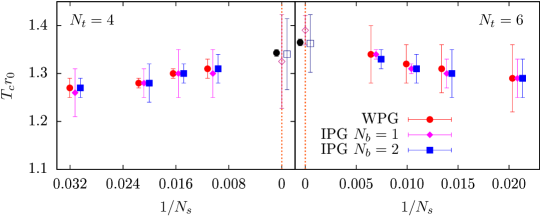
Figure 12: Results for the deconfinement transition temperatures $T_{c}r_{0}$ vs the inverse box length $1/N_{s}$ for $N_{t}=4$ (left) and $N_{t}=6$ (right). The data have been slightly displaced to improve the visibility of the different sets of points. The black data point at $1/N_{s}=0$ is the result in the infinite-volume limit from the Bielefeld group Engels:1996dz , while the magenta and blue open symbols are the results for $T_{c}(\infty)$ from IPG with $N_{b}=1$ and 2, respectively.

5.3 Order and universality class of the transition

Owing to the scaling of $T_{c}$ discussed above, we expect the transitions in IPG and WPG to be in the same universality class. Moreover, as already discussed in section 2, center symmetry is a good symmetry for both actions so that the deconfinement transition is accompanied by center-symmetry breaking. Another strong indication for the transitions being in the same universality class comes from the similar volume scaling of the susceptibility peaks of the Polyakov loop (cf. figures 10 and 11). We will now test whether these expectations are correct and both transitions are indeed in the 2d Ising universality class, which is known to be the case at least for 3d $\text{SU}(2)$ WPG theory Engels:1996dz .

There are several types of analyses one can employ to determine the critical exponents which distinguish the different universality classes. Here we follow the strategy of Engels:1996dz and use the $\chi^{2}$-method Engels:1992ke . The starting point is the finite-size scaling formula for the susceptibility of the Polyakov loop expanded around the critical point,

$$\chi_{L}=N_{s}^{\gamma/\nu}\Big{(}c_{0}+\Big{(}c_{1}+c_{2}N_{s}^{-\gamma_{i}}\Big{)}\tau N_{s}^{1/\nu}+c_{3}N_{s}^{-\gamma_{i}}\Big{)}.$$ (29)

Here, $c_{0,1,2}$ are unknown coefficients, $\gamma_{i}$ is an unknown exponent,

$$\tau=\frac{T_{c}(\infty)-T}{T_{c}(\infty)}$$ (30)

is the reduced temperature with respect to the critical temperature in the thermodynamic limit $T_{c}(\infty)$, $N_{s}$ is the spatial extent of the lattice, and $\gamma/\nu$ is the desired ratio of critical exponents. Exactly at $T_{c}(\infty)$, eq. (29) reduces to

$$\chi_{L}=N_{s}^{\gamma/\nu}\left(c_{0}+c_{3}N_{s}^{-\gamma_{i}}\right).$$ (31)

At large $N_{s}$ the second term (proportional to $c_{3}$) is a correction and can be neglected. We thus arrive at the scaling relation

$$\ln(\chi_{L})=C+\frac{\gamma}{\nu}\ln(N_{s})\,.$$ (32)

This scaling law can be tested by fitting the data at a given coupling to (32). Since at $T\neq T_{c}(\infty)$ there are corrections of the form given in eq. (29), we will get the best fit when the coupling is equal (or very close) to the critical coupling. The critical temperature $T_{c}(\infty)$ can thus be extracted by looking at $\chi^{2}/$dof, in principle.

The main problem of this analysis is the finite resolution of simulation points in the region around $T_{c}$ and the different accuracy of the results for the susceptibility. For WPG theory this problem can be overcome by the use of the multi-histogram method Ferrenberg:1988yz , which can be used for a well-controlled interpolation between simulation points. In addition, the method leads to enhanced and balanced statistics for all simulation points. In IPG theory this method cannot be applied since $\alpha$, unlike $\beta$, does not appear as a simple prefactor in front of an observable (the average plaquette for WPG) in the action. For IPG this leads to the problem that $\chi^{2}/$dof fluctuates strongly and cannot be used as a conclusive indicator for $T_{c}$ as in Engels:1996dz . Instead, we will compare to the results for $\gamma/\nu$ obtained for the individual temperatures by fitting to eq. (32) and making use of the results for $T_{c}(\infty)$ from table 10. In this way we obtain a number of possible results for $\gamma/\nu$ in the region of $T_{c}(\infty)$. To be conservative, we use the full spread of results as the uncertainty interval which encloses the final result for $\gamma/\nu$ and define the central value of our final result to be the midpoint of this interval. These results are also listed in table 10. Unfortunately, the uncertainties in IPG are too large to draw definite conclusions from the comparison. Nonetheless, the results are in agreement with those of WPG within errors.

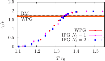
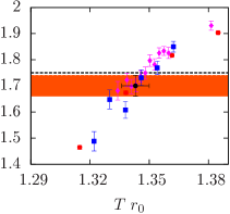
Figure 13: Results for $\gamma/\nu$ from the fits discussed in the text, for 3d $\text{SU}(2)$ gauge theory at $N_{t}=4$. The plot on the right displays the details of the $T_{c}(\infty)$ region. The black dashed line is the prediction for $\gamma/\nu$ from a reduced model (RM) (cf. Engels:1996dz ) and the black data point, together with the orange band, the result from the Bielefeld group Engels:1996dz .

The results of the analysis are shown in figures 13 and 14 for $N_{t}=4$ and 6, respectively. The plot on the right in the figures shows the details in the region around $T_{c}r_{0}(\infty)$. In the plots we do not show the results for $\gamma/\nu$ in IPG since the uncertainties are rather large. However, when we assume that a hypothetical high-precision result for $T_{c}(\infty)$ in IPG would be similar to the result in WPG, the plot indicates that we would get a similar result for $\gamma/\nu$, too. All in all we have compelling evidence that the transitions in WPG and IPG theory are in the same universality class. Moreover, cutoff effects are similar, so that we can expect this statement to be true for the continuum limit as well.

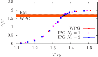
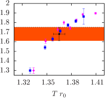
Figure 14: Same as figure 13 but for $N_{t}=6$.

6 Conclusions

In this paper we have tested the conjecture of the equivalence of the continuum limit of induced pure gauge theory, formulated originally by Budczies and Zirnbauer in Budczies:2003za , and pure gauge theory with Wilson’s gauge action Wilson:1974sk . To this end we have performed simulations with both discretizations in three dimensions with gauge group $\text{SU}(2)$ at matched couplings to achieve similar lattice spacings. The matching via the Sommer scale was discussed in detail in section 3. It is found to be in good agreement with perturbation theory, both concerning its functional form and the numerical results for the matching coefficients (see also (Brandt:2016duy, , sec. 4.3) and appendix B).

Using the matching, we have performed simulations at similar lattice spacings for a high-precision comparison of observables. In particular, we have looked at the leading and subleading properties of the static $q\bar{q}$ potential at intermediate and long distances in section 4. The leading properties are characterized by the string tension and the subleading ones by the non-universal boundary coefficient $\bar{b}_{2}$. Both observables show excellent agreement between WPG and IPG in the approach to the continuum for $N_{b}=1$ and $N_{b}=2$ and are similar already at finite lattice spacing. This indicates that the continuum potential is identical, at least at the current level of precision.

The thermodynamic properties of IPG theory have been investigated in section 5 for two temporal extents, $N_{t}=4$ and 6. Once more the agreement between the two theories for the behavior of the Polyakov loop and its susceptibility is remarkable for all volumes and over the full range of temperatures. Accordingly, the ratio of critical exponents $\gamma/\nu$ agrees very well with the known result for WPG from the Bielefeld group Engels:1996dz , indicating that the transition in both theories is in the same universality class. Furthermore, the transition temperature in the thermodynamic limit is also in agreement, which is another important crosscheck since $T_{c}$ is a non-universal quantity.

One of the problems of the Kazakov-Migdal model Kazakov:1992ym , an earlier model supposed to induce Yang-Mills theory, is the existence of a local center symmetry which constrains all Wilson lines to vanish. The present model for induced Yang-Mills theory does not have this problem. This is also reflected in the results for the Polyakov loop obtained in section 5. The results for the Polyakov loop fall in the two sectors singled out by the center symmetry of $\text{SU}(2)$, i.e., they are located around $|L|$ and $-|L|$ on the real axis. This shows that the model also recovers the correct symmetry, whose breaking is associated with the transition in Yang-Mills theory. As mentioned already in section 2, this is also expected from the symmetries of the weight factor, eq. (1).

Concerning numerical efficiency, our simulations of IPG theory are up to a factor of 100 slower than the associated simulations in WPG theory, depending on the bare parameters in the simulations. We would like to stress that this inefficiency is an attribute of the choice of the simulation algorithm alone, as explained in detail in appendix A. We are confident that one can find an algorithm similar to the heat-bath algorithm for WPG Kennedy:1985nu , which should then lead to a similar performance. In particular, if one is interested in simulations including fermionic degrees of freedom, the Hybrid Monte Carlo (HMC) algorithm Duane:1987de is supposedly the algorithm of choice. We have tested the HMC algorithm for IPG theory in its bosonized version and found it to perform almost as well as the HMC for WPG theory in both $\text{SU}(2)$ gauge theory for $d=3$ and $\text{SU}(3)$ in four dimensions. A general problem working in the bosonized version is the increase in autocorrelations, which can be enhanced up to an order of magnitude. However, this is compensated to some extent by the speed-up of the individual HMC steps. It is interesting to note that the HMC algorithm for IPG theory can be set up in such a way that the auxiliary boson fields are drawn from the exact distribution for the starting configuration. In this case no communication is needed to evolve the link variables in pure gauge theory, which results in a very efficient parallelization.

All in all, we find that the results from the two theories agree very well already away from the continuum limit and that the agreement improves as the continuum limit is approached. This is true already for $N_{b}=1$, which leads us to conclude that the bound in eq. (3) can indeed be relaxed for $d>2$. Our results thus support the universality argument given in Budczies:2003za . Therefore the modified BZ method, combined with a suitable strong-coupling approach, can be used to reformulate lattice gauge theories in a number of different ways. We leave these reformulations for future work.

Appendix A Simulation details

A.1 Update algorithm

The weight for a link $U_{\mu}(x)$ in the weight factor (1) in IPG theory is local so that we can use a local version of the Metropolis algorithm Metropolis:1953am for the simulations. More precisely, we propose a new link $U^{\prime}_{\mu}(x)$ and accept it with probability

$$P=\min\Bigg{\{}1,\Bigg{[}\prod_{p}\frac{\det\big{(}1-\frac{\alpha}{2}\big{(}U_{p}+U_{p}^{\dagger}\big{)}\big{)}}{\det\big{(}1-\frac{\alpha}{2}\big{(}U^{\prime}_{p}+{U^{\prime}_{p}}^{\dagger}\big{)}\big{)}}\Bigg{]}^{N_{b}}\Bigg{\}}\,.$$ (33)

Here, the product over $p$ is taken over all plaquettes that include the link $U_{\mu}(x)$, $U_{p}$ denotes the plaquette including the old link $U_{\mu}(x)$, and $U^{\prime}_{p}$ the plaquette including the new link $U^{\prime}_{\mu}(x)$. The crucial part affecting the efficiency of the algorithm is to find new links $U^{\prime}_{\mu}(x)$ that lead to a large acceptance rate in the step defined by eq. (33). Since in our pilot study of IPG theory efficiency of the algorithm was not our primary concern, we simply took the new links $U^{\prime}_{\mu}(x)$ to be random $\text{SU}(2)$ matrices in an $\epsilon$-surrounding of the old links $U_{\mu}(x)$. In practice, we have generated a random element $X=\sum_{a}x^{a}T^{a}\in\text{su}(2)$ (the Lie algebra of $\text{SU}(2)$), where the $T^{a}$ are the generators of $\text{SU}(2)$ and the coefficients $x^{a}$ are taken from the interval $[-\epsilon,\epsilon]$, and constructed the new link via $U^{\prime}_{\mu}(x)=\exp(X)U_{\mu}(x)$. To make sure that in each step a sufficient number of links is updated, we have tuned $\epsilon$ so that the overall acceptance rate is around 80%. To further decorrelate two measurements we have separated them by $N_{\text{sw}}$ sweeps, where $N_{\text{sw}}$ is chosen to be much larger than the integrated autocorrelation time in units of lattice sweeps.

A.2 Extraction of the static $q\bar{q}$ potential

To compare the two theories we mostly use quantities that are related to the potential between a static quark and antiquark. The cleanest way, in terms of excited-state contaminations, to extract the potential in numerical simulations is given by measuring the correlation function of two Polyakov loops, $L(\vec{x})$, defined by (cf. eq. (26))

$$L(\vec{x})=\operatorname{\text{Tr}}\prod_{n_{0}=1}^{N_{t}}U_{0}(n_{0}\,a,\vec{x})\,,$$ (34)

where $n_{0}$ denotes the temporal coordinate, $N_{t}$ is the number of lattice points in the temporal direction, and $\vec{x}$ is the vector including the spatial coordinates. The spectral representation of a correlation function of two Polaykov loops separated by a distance $R$ is given by

$$\left\langle L^{\ast}(R)\>L(0)\right\rangle=\sum_{n=0}^{\infty}b_{n}\>e^{-E_{n}(R)\>T}$$ (35)

for $R\ll L/2$, where $T=aN_{t}$ and $L=aN_{s}$ are the temporal and spatial extents of the lattice, $b_{i}$ denotes the overlap between the operator and the energy eigenstate, and $E_{n}(R)$ is the $n$-th energy level. Here the energies are ordered in ascending order, i.e., $E_{0}<E_{1}<E_{2}<\ldots\;$. In the limit $T\to\infty$ the right-hand side of eq. (35) is dominated by the ground state with $E_{0}(R)=V(R)$. Excited states are suppressed exponentially with $\exp\{-[E_{i}(R)-E_{0}(R)]T\}$. This means that excited states can be neglected for large values of $T$. In this case we can extract $V(R)$ via

$$V(R)=-\frac{1}{T}\ln\left[\left\langle L^{\ast}(R)\>L(0)\right\rangle\right].$$ (36)

The correlation functions in eq. (35) suffer from a well-known exponential decay of the signal-to-noise ratio with the area enclosed by the two loops. This renders the extraction of the potential difficult for large $R$. For simulations in WPG this problem can be overcome by the use of a multilevel algorithm introduced by Lüscher and Weisz Luscher:2001up . The same algorithm can also be applied in IPG since the locality properties of the action are similar to those of the plaquette action. The details are discussed in appendix A.3.

A suitable observable to set the scale with the static potential is the Sommer parameter $r_{0}$ Sommer:1993ce , which is defined implicitly by

$$r_{0}^{2}F(r_{0})=1.65\,,$$ (37)

where $F(R)$ is the force

$$F(R)\equiv\frac{\partial V(R)}{\partial R}\,.$$ (38)

To extract $r_{0}/a$ we use the following four methods (see also Brandt:2017yzw ):

1. a numerical polynomial interpolation of $R^{2}F(R)$,

2. a numerical rational interpolation of $R^{2}F(R)$,

3. a parameterization of the form Sommer:1993ce

   $$F(R)=f_{0}+\frac{f_{1}}{R^{2}}+\frac{f_{2}}{R^{4}}$$ (39)

   for the values of $R$ corresponding to the four nearest neighbors of $r_{0}$ (motivated by the EST to LO),

4. the parameterization of (39) with $f_{2}=0$ for the two nearest neighbors of $r_{0}$.

The final estimate for $r_{0}/a$ is obtained from method (d), while methods (a) to (c) are used to compute the systematic uncertainty associated with the interpolation.

A.3 Error reduction for large loops

A suitable algorithm to overcome the exponential decay of the signal-to-noise ratio for large loops is the multilevel algorithm proposed by Lüscher and Weisz Luscher:2001up . The algorithm relies on a key property of the theory, the locality of the configuration weight, which ensures that sublattices, i.e., lattice domains separated by a time slice with fixed spatial links, are independent during local updates. IPG theory also has this form of locality since, as for the Wilson action, the weight for a particular link $U_{\mu}(x)$ only depends on the plaquettes including this link. The error-reduction efficiency of the algorithm, however, depends on the properties of the transfer matrix since this is the object for which the uncertainty is decreased in the course of the sublattice updates. If we are close enough to the continuum and both theories indeed approach the same continuum limit, we can expect the transfer matrix to be similar in both theories (given by the continuum result plus lattice artifacts) so that the algorithm should lead to a comparable error reduction also in the case of IPG theory.

A way to estimate the amount of error reduction for Polyakov-loop correlation functions, and thereby the optimal number of sublattice updates for loops of a particular size, has been proposed in Majumdar:2002ga . Following this proposal we define the norm $N(R)$ of a local two-link operator with link separation $R$ on a particular sublattice as in (Majumdar:2002ga, , eq. (4)). The two-link operator plays the role of a transfer matrix for Polyakov-loop correlators Luscher:2001up . The decay of $N(R)$ provides an estimate for the residual fluctuations of the transfer matrix. For a large number $n_{t}$ of sublattice updates we expect $N(R)$ to fall off as $1/\sqrt{n_{t}}$.

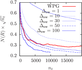
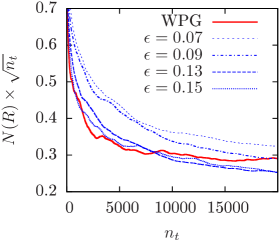
Figure 15: Results for the norm $N(R)$ from Majumdar:2002ga multiplied by the square root of the number of measurements in WPG and IPG with $N_{b}=2$ for the cases $R=10$ and $\epsilon=0.07$ (left) with different numbers $\Delta_{\text{sw}}$ of sublattice updates between two measurements, and $R=10$ and $\Delta_{\text{sw}}=15$ (right) with different values of $\epsilon$.

To compare the error-reduction efficiency of the algorithm in the IPG and WPG theories we have performed dedicated simulations in the $\text{SU}(2)$ theory on a $24^{3}$ lattice at $\beta=5.0$ and the roughly equivalent $\alpha=0.65$ in IPG with $N_{b}=2$. We have fixed the temporal extent $t_{s}$ of the sublattices to 2 throughout and measured two-link operators with link separations between 2 and 10. In figure 15 we show the results for link separation 10. The “optimal” value of $n_{t}$ is taken to be the point at which the expected asymptotic behavior $N(R)\sim 1/\sqrt{n_{t}}$ sets in for the largest value of $R$ considered. After this point no further exponential error reduction is achieved.

The plot indicates that for WPG theory $n_{t}=15000$ to 20000 is sufficient. For IPG theory, $N(R)\times\sqrt{n_{t}}$ decreases more slowly if we perform measurements at each sublattice update. The main reason is that the sublattice configurations after one sublattice sweep of local Metropolis updates in IPG theory are more correlated than the configurations after one sublattice sweep of heat-bath updates for WPG theory. We therefore separate the measurements in IPG theory by $\Delta_{\text{sw}}$ sublattice sweeps (which saves simulation time since the measurement of the observable is more costly than a sweep of Metropolis updates). We see from figure 15 (left) that the decay of the norm becomes stronger when we increase $\Delta_{\text{sw}}$. For the values shown in figure 15 (left), where $\epsilon=0.07$, $\Delta_{\text{sw}}=50-100$ appears to be a good choice. Moreover, the optimal value of $\Delta_{\text{sw}}$ depends on the value of $\epsilon$, as shown in figure 15 (right). Since in the final simulations we have used a value of $\epsilon=0.14$, for which the integrated autocorrelation time is a factor of 3 smaller than for $\epsilon=0.07$, the optimal value of $\Delta_{\text{sw}}$ can be taken to be around 20 for $\alpha=0.65$. A similar tuning can be done for the other $\alpha$-values in the simulation. Since the optimal values of $\epsilon$ and $\Delta_{\text{sw}}$ at a particular lattice spacing are a property of the algorithm, we can use the same setup for other values of $N_{b}$ as long as we have tuned $\alpha$ so that we simulate at similar lattice spacings. Note that the correctness of the algorithm does not depend on the particular values of $\epsilon$ and $\Delta_{\text{sw}}$. The only effect of a suboptimal tuning of $\epsilon$ or $\Delta_{\text{sw}}$ is less error reduction.

Appendix B Comparison of the matching with perturbation theory

We want to compare the matching between the lattice couplings $\beta$ and $\alpha$ discussed in section 3.2 to the perturbative results for the matching obtained in Brandt:2016duy . The perturbative result (after analytic continuation to the region where $\alpha\to 1$) as given in (Brandt:2016duy, , eq. (4.15)), reformulated in terms of the lattice couplings $\beta$ and $\alpha$, is given by

$$\beta=d_{0}(N_{b})N_{c}\frac{\alpha}{1-\alpha}\Big{(}1+d_{1}(N_{b})\frac{2(1-\alpha)}{d_{0}(N_{b})\,\alpha}+\mathcal{O}((1-\alpha)^{2})\Big{)}.$$ (40)

The $N_{b}$-dependence of $d_{0}(N_{b})$ and $d_{1}(N_{b})$ can be computed in perturbation theory in the limit $N_{b}\to\infty$. For a direct comparison to perturbation theory it is convenient to replace the matching function from eq. (12) by

$$\beta(\alpha)=d_{0}(N_{b})N_{c}\frac{\alpha}{1-\alpha}+\tilde{b}_{0}+\tilde{b}_{1}\frac{(1-\alpha)}{\alpha}\,.$$ (41)

We are particularly interested in the coefficient $d_{0}$, for which the perturbative prediction is given in (Brandt:2016duy, , eq. (4.78)).

To compare to perturbation theory we have used the parameterization (41) for a comparison with the data for $N_{b}=1$ and 2 from section 3.2 and performed additional simulations for $N_{b}=3$, 4 and 5, for which the simulation parameters are listed in table 11. We observe that this parameterization works well and leads to a similar description of the data as the parameterization used in section 3.2. The results for $d_{0}(N_{b})/N_{b}$, which have already been shown in (Brandt:2016duy, , Figure 2), are listed in table 12. For the comparison itself we refer to Brandt:2016duy .

$N_{b}$	$\alpha$	size	$R$	$t_{s}$	$n_{t}$	$\Delta_{\text{sw}}$	meas	$N_{\text{sw}}$	$\epsilon$	$r_{0}$
3	0.50	$24^{3}$	1-9	2	100k	20	2000	1000	0.14	3.269(1)(1)
	0.60	$36^{3}$	1-10	4	200k	40	2000	1500	0.10	5.349(1)(1)
	0.70	$48^{3}$	1-11	6	500k	100	1900	2000	0.08	8.679(2)(1)
4	0.42	$24^{3}$	1-10	2	100k	20	2000	1000	0.14	3.506(1)(1)
	0.51	$36^{3}$	1-11	4	200k	40	2000	1500	0.10	5.417(1)(1)
	0.60	$48^{3}$	1-11	6	500k	100	1800	2000	0.08	8.143(2)(1)
5	0.38	$24^{3}$	1-9	2	100k	20	1900	1000	0.14	4.004(1)(4)
	0.49	$36^{3}$	1-11	4	200k	40	2000	1500	0.10	6.733(2)(7)
	0.55	$48^{3}$	1-12	6	500k	100	2300	2000	0.08	8.775(4)(1)

Table 11: Simulation parameters and results for the measurements of $r_{0}$ in pure $\text{SU}(2)$ IPG for $N_{b}=3$, 4 and 5. Here, $R$ gives the range of $q\bar{q}$ separations used in the analysis of Polyakov-loop correlation functions, $t_{s}$ is the temporal extent of the Lüscher-Weisz sublattices, $n_{t}$ is the number of sublattice updates, $\Delta_{\text{sw}}$ is the number of sweeps separating two sublattice measurements, $N_{\text{sw}}$ is the number of sweeps between two measurements, and $\epsilon$ is the size of the ball for the link proposal. For more details on the algorithms, e.g., the choice of $\Delta_{\text{sw}}$ and $N_{\text{sw}}$, see appendix A.

We can also compare directly to the matching results of section 3.2 by noting that the coefficients $b_{-1}$ and $d_{0}$ are related by

$$d_{0}(N_{b})=b_{-1}(N_{b})/N_{c}\,.$$ (42)

Using this relation to convert the results of eq. (13) for $b_{-1}(N_{b})$ with $N_{b}=1$ and 2 to results for $d_{0}$ gives

$$d_{0}(1)/N_{b}=0.312(2)\quad\text{and}\quad d_{0}(2)/N_{b}=0.613(4)\,,$$ (43)

in perfect agreement with the results in table 12.

$N_{b}$	1	2	3	4	5
$d_{0}/N_{b}$	0.311(2)	0.614(3)	0.735(3)	0.793(3)	0.847(6)

Table 12: Numerical results for the perturbative coefficient $d_{0}(N_{b})$, normalized by $N_{b}$.

References

- (1) J. Blairon, R. Brout, F. Englert, and J. Greensite, Chiral Symmetry Breaking in the Action Formulation of Lattice Gauge Theory, Nucl.Phys. B180 (1981) 439.
- (2) H. Kluberg-Stern, A. Morel, O. Napoly, and B. Petersson, Spontaneous Chiral Symmetry Breaking for a U(N) Gauge Theory on a Lattice, Nucl.Phys. B190 (1981) 504.
- (3) N. Kawamoto and J. Smit, Effective Lagrangian and Dynamical Symmetry Breaking in Strongly Coupled Lattice QCD, Nucl.Phys. B192 (1981) 100.
- (4) P. Rossi and U. Wolff, Lattice QCD With Fermions at Strong Coupling: A Dimer System, Nucl.Phys. B248 (1984) 105.
- (5) F. Karsch and K. Mutter, Strong coupling QCD at finite baryon number density, Nucl.Phys. B313 (1989) 541.
- (6) M. Bander, Equivalence of Lattice Gauge and Spin Theories, Phys.Lett. B126 (1983) 463.
- (7) H. W. Hamber, Lattice gauge theories at large N(f), Phys.Lett. B126 (1983) 471.
- (8) V. Kazakov and A. A. Migdal, Induced QCD at large N, Nucl.Phys. B397 (1993) 214–238, [hep-th/9206015].
- (9) A. Hasenfratz and P. Hasenfratz, The Equivalence of the SU(N) Yang-Mills theory with a purely fermionic model, Phys.Lett. B297 (1992) 166–170, [hep-lat/9207017].
- (10) J. Budczies and M. Zirnbauer, Howe duality for an induced model of lattice U(N) Yang-Mills theory, math-ph/0305058.
- (11) B. B. Brandt, R. Lohmayer, and T. Wettig, Induced QCD I: Theory, JHEP 11 (2016) 087, [1609.06466].
- (12) R. Sommer, A New way to set the energy scale in lattice gauge theories and its applications to the static force and alpha-s in SU(2) Yang-Mills theory, Nucl.Phys. B411 (1994) 839–854, [hep-lat/9310022].
- (13) H. Vairinhos and P. de Forcrand, Lattice gauge theory without link variables, JHEP 12 (2014) 038, [1409.8442].
- (14) B. B. Brandt and T. Wettig, Induced QCD with two auxiliary bosonic fields, PoS LATTICE2014 (2015) 307, [1411.3350].
- (15) B. B. Brandt, R. Lohmayer, and T. Wettig, Induced YM Theory with Auxiliary Bosons, PoS LATTICE2015 (2016) 276, [1511.08374].
- (16) K. G. Wilson, Confinement of Quarks, Phys.Rev. D10 (1974) 2445–2459.
- (17) A. Kennedy and B. Pendleton, Improved Heat Bath Method for Monte Carlo Calculations in Lattice Gauge Theories, Phys.Lett. B156 (1985) 393–399.
- (18) M. Creutz, Overrelaxation and Monte Carlo Simulation, Phys.Rev. D36 (1987) 515.
- (19) N. Metropolis, A. Rosenbluth, M. Rosenbluth, A. Teller, and E. Teller, Equation of state calculations by fast computing machines, J.Chem.Phys. 21 (1953) 1087–1092.
- (20) P. Majumdar, Continuum limit of the spectrum of the hadronic string, hep-lat/0406037.
- (21) N. Hari Dass and P. Majumdar, Continuum limit of string formation in 3-d SU(2) LGT, Phys.Lett. B658 (2008) 273–278, [hep-lat/0702019].
- (22) B. B. Brandt and P. Majumdar, Spectrum of the QCD flux tube in 3d SU(2) lattice gauge theory, Phys.Lett. B682 (2009) 253–258, [0905.4195].
- (23) B. B. Brandt, Probing boundary-corrections to Nambu-Goto open string energy levels in 3d SU(2) gauge theory, JHEP 1102 (2011) 040, [1010.3625].
- (24) B. B. Brandt, Spectrum of the open QCD flux tube in d=2+1 and its effective string description, 1308.4993.
- (25) B. B. Brandt, Spectrum of the open QCD flux tube and its effective string description I: 3d static potential in SU(N = 2, 3), JHEP 07 (2017) 008, [1705.03828].
- (26) B. B. Brandt, Spectrum of the open QCD flux tube and its effective string description, in 13th Conference on Quark Confinement and the Hadron Spectrum (Confinement XIII) Maynooth, Ireland, July 31-August 6, 2018, 2018. 1811.11779.
- (27) B. B. Brandt and M. Meineri, Effective string description of confining flux tubes, Int. J. Mod. Phys. A31 (2016), no. 22 1643001, [1603.06969].
- (28) O. Aharony and Z. Komargodski, The Effective Theory of Long Strings, JHEP 1305 (2013) 118, [1302.6257].
- (29) J. Arvis, The Exact Potential in Nambu String Theory, Phys.Lett. B127 (1983) 106.
- (30) O. Aharony and N. Klinghoffer, Corrections to Nambu-Goto energy levels from the effective string action, JHEP 1012 (2010) 058, [1008.2648].
- (31) O. Aharony, M. Field, and N. Klinghoffer, The effective string spectrum in the orthogonal gauge, JHEP 1204 (2012) 048, [1111.5757].
- (32) S. Dubovsky, R. Flauger, and V. Gorbenko, Effective String Theory Revisited, JHEP 1209 (2012) 044, [1203.1054].
- (33) S. Dubovsky, R. Flauger, and V. Gorbenko, Flux Tube Spectra from Approximate Integrability at Low Energies, J. Exp. Theor. Phys. 120 (2015), no. 3 399–422, [1404.0037].
- (34) A. M. Polyakov, Confining strings, Nucl. Phys. B486 (1997) 23–33, [hep-th/9607049].
- (35) H. Panagopoulos, A. Skouroupathis, and A. Tsapalis, Free energy and plaquette expectation value for gluons on the lattice, in three dimensions, Phys.Rev. D73 (2006) 054511, [hep-lat/0601009].
- (36) J. Engels, F. Karsch, E. Laermann, C. Legeland, M. Lutgemeier, et al., A Study of finite temperature gauge theory in (2+1)-dimensions, Nucl.Phys.Proc.Suppl. 53 (1997) 420–422, [hep-lat/9608099].
- (37) F. Y. Wu, The Potts model, Rev. Mod. Phys. 54 (1982) 235–268. [Erratum: Rev. Mod. Phys.55,315(1983)].
- (38) J. Liddle and M. Teper, The Deconfining phase transition in D=2+1 SU(N) gauge theories, 0803.2128.
- (39) J. Engels, J. Fingberg, and V. Mitrjushkin, Efficient calculation of critical parameters in SU(2) gauge theory, Phys.Lett. B298 (1993) 154–158.
- (40) A. Ferrenberg and R. Swendsen, New Monte Carlo Technique for Studying Phase Transitions, Phys.Rev.Lett. 61 (1988) 2635–2638.
- (41) S. Duane, A. Kennedy, B. Pendleton, and D. Roweth, Hybrid Monte Carlo, Phys.Lett. B195 (1987) 216–222.
- (42) M. Luscher and P. Weisz, Locality and exponential error reduction in numerical lattice gauge theory, JHEP 0109 (2001) 010, [hep-lat/0108014].
- (43) P. Majumdar, Experiences with the multilevel algorithm, Nucl.Phys.Proc.Suppl. 119 (2003) 1021–1023, [hep-lat/0208068].