Toward convergence of effective field theory simulations on digital quantum computers

Abstract

We report results for simulating an effective field theory to compute the binding energy of the deuteron nucleus using a hybrid algorithm on a trapped-ion quantum computer. Two increasingly complex unitary coupled-cluster ansaetze have been used to compute the binding energy to within a few percent for successively more complex Hamiltonians. By increasing the complexity of the Hamiltonian, allowing more terms in the effective field theory expansion and calculating their expectation values, we present a benchmark for quantum computers based on their ability to scalably calculate the effective field theory with increasing accuracy. Our result of $E_{4}=-2.220\pm 0.179$MeV may be compared with the exact Deuteron ground-state energy $-2.224$MeV. We also demonstrate an error mitigation technique using Richardson extrapolation on ion traps for the first time. The error mitigation circuit represents a record for deepest quantum circuit on a trapped-ion quantum computer.

I Introduction

Simulating Fermonic matter using quantum computers has recently become an active field of research. With the advent of noisy intermediate-scale quantum (NISQ) devices that are capable of processing quantum information, hybrid quantum-classical computing (HQCC) has been proposed to be a worthy strategy to harness the advantage quantum computers provide as early as possible. A host of HQCC demonstrations, ranging from its application in chemistry O’Malley et al. (2016); Kandala et al. (2017); Nam et al. (2019) to machine learning Benedetti et al. (2018), are in fact already available in the literature.

NISQ devices are however susceptible to errors and defects. Thus, the quantum circuits to be run on these machines need to be sufficiently small so that the results that the quantum computers output are still useful. On the other hand, in order for the quantum computational results to be useful, the computation that the quantum computer performs needs to be sufficiently demanding such that readily available classical devices cannot easily arrive at the same results. However, there is a lack of empirical evidence for the performance scaling of HQCC as problems become more complex. A test, or benchmark, of this scalability would be useful to inform future quantum algorithm development.

Here, using the effective field theory (EFT) simulation of a deuteron, we outline a path to scalable HQCC and provide a benchmark that determines the HQCC performance scaling of a quantum computer. We further demonstrate that a trapped-ion quantum computer today is capable of addressing small, yet scalable HQCC problems, and that it shows promises toward scaling to reliable computational results when a quantum advantage is demonstrated.

We also demonstrate a re-parametrization technique that yields a quantum circuit amenable to implementation on quantum computers with nearest-neighbor connectivity. We report our experimental results that leverage known error mitigation techniques Temme et al. (2017); Li and Benjamin (2017); Endo et al. (2018); McArdle et al. (2018). The theoretical predictions for the three- and four-qubit case are within the error bars of the experimental results.

II Hamiltonian and Ansätz

The $N$ oscillator-basis deuteron Hamiltonian we consider (see Supplementary material for detail) is

$$H_{N}=\sum_{n,n^{\prime}=0}^{N-1}\langle n^{\prime}|(T+V)|n\rangle a^{\dagger}_{n^{\prime}}a_{n},$$ (1)

where the operators $a^{\dagger}_{n}$ and $a_{n}$ create and annihilate a deuteron in the harmonic-oscillator $s$-wave state $|n\rangle$ and the matrix elements of the kinetic and potential energy are

$$\langle n^{\prime}|T|n\rangle = {\hbar\omega\over 2}\bigg{[}(2n+3/2)\delta^{n^{\prime}}_{n}-\sqrt{n(n+1/2)}\delta_{n}^{n^{\prime}+1}$$

$$-\sqrt{(n+1)(n+3/2)}\delta_{n}^{n^{\prime}-1}\bigg{]},$$

$$\langle n^{\prime}|V|n\rangle = V_{0}\delta_{n}^{0}\delta^{n^{\prime}}_{n},$$ (2)

where $\hbar\omega\approx 7\,{\rm MeV}$ and $V_{0}\approx-5.68\,{\rm MeV}$. Since our goal is to find the ground state energy expectation values as a function of $N$ using a quantum computer, we apply Jordan-Wigner transform Jordan and Wigner (1993) to our physical Hamiltonian in (1) to find the qubit Hamiltonian. For $N=2,3,$ and $4$, we have

$$H_{2} = 5.907I+0.218Z_{0}-6.125Z_{1}-2.143(X_{0}X_{1}+Y_{0}Y_{1})$$

$$H_{3} = H_{2}+9.625(I-Z_{2})-3.913(X_{1}X_{2}+Y_{1}Y_{2})$$

$$H_{4} = H_{3}+13.125(I-Z_{3})-5.671(X_{2}X_{3}+Y_{2}Y_{3}).$$ (3)

For our current example of a Deuteron EFT simulation, the UV cutoff determines the largest matrix element in the nuclear Hamiltonian, which controls the scaling of the coefficients of the Pauli terms in the qubit Hamiltonian in (II). Since the uncertainty in determining the expectation value of the Hamiltonian is bounded by the largest absolute value of the coefficients in the qubit Hamiltonian Kandala et al. (2017), the higher the UV cutoff, the larger the uncertainty in the expectation value of the Hamiltonian becomes. To meet the required, preset uncertainty, we need to make a larger number of measurements for a large-coefficient Hamiltonian. Because the largest coefficient tends to grow with basis size, this effectively induces an implementation-level tug-of-war between the increasingly accurate simulation from considering a larger oscillator basis and the accumulation of errors on NISQ devices susceptible to, e.g., drifts, that occur over the required, longer overall runtime. While frequently calibrating the quantum computer may help reduce the errors, this may not be desirable as it would significantly increase the resource overhead.

For the HQCC ansatz, we use the $N$-site unitary coupled-cluster singles (UCCS) ansatz

$$|\Psi_{\text{UCCS}}\rangle=\exp\left(\sum\limits_{k=1}^{N-1}\theta_{k}[a^{\dagger}_{0}a_{k}-a^{\dagger}_{k}a_{0}]\right)|1_{0}\rangle,$$ (4)

where $\vec{\theta}=\{\theta_{1},...,\theta_{N-1}\}$ is the set of $N-1$ real-valued variational parameters and $|1_{i}\rangle$ denotes the state $|0,...,0,1,0,...,0\rangle$ with the $i$th $s$-wave state occupied. We compute the deuteron binding energy by minimizing the quantum functional $\langle\Psi_{\text{UCCS}}|H_{N}|\Psi_{\text{UCCS}}\rangle$ with respect to $\vec{\theta}$. The initial state $|1_{0}\rangle=|1,0,0,...0\rangle$ represents the occupation of the 0th $s$-wave state.

To implement the UCCS ansatz on our quantum computer, we re-parameterized (4) in the hyper-spherical coordinate, i.e.,

$$|\Psi_{\text{UCC}}\rangle = \sum\limits_{k=0}^{N-2}\cos(\lambda_{k})\tilde{|1_{k}\rangle}+\tilde{|1_{N-1}\rangle},$$ (5)

where $\tilde{|1_{k}\rangle}\equiv\prod\limits_{i=0}^{k-1}\sin(\lambda_{i})|1_{k}\rangle$ with $\tilde{|1_{0}\rangle}=|1_{0}\rangle$. This choice is deliberate and exact, since the excitation operator in (4) is solely composed of single-excitations. Note we have relabeled (and re-indexed) variational parameters as $\vec{\lambda}=\{\lambda_{0},...,\lambda_{N-2}\}$.

With the new parameterization shown in (5), we may now synthesize the ansatz circuit straightforwardly. Let us define the amplitude shifting unitary $U_{i,i+1}(\lambda_{i})\equiv(C_{i+1}X_{i})(C_{i}RY_{i+1}(\lambda_{i}))$, where $C_{m}G_{n}$, for instance, denotes a single-qubit gate $G$ acting on qubit $n$, controlled by qubit $m$, such that $U(\lambda)(\alpha|00\rangle+\beta|10\rangle)=\alpha|00\rangle+\beta(\cos{\lambda}|10\rangle+\sin{\lambda}|01\rangle$). Applying $U_{i,i+1}$ in series to an initial state of $|1_{0}\rangle$, we have

$$|\Psi_{\text{UCC}}\rangle=\left[\prod_{i=0}^{N-2}U_{i,i+1}(\lambda_{i})\right]|1_{0}\rangle.$$ (6)

For the first non-trivial case of $N=2$, we need to optimize $U_{0,1}$ acting on $|1_{0}\rangle$. Since the initial state is $|10\rangle$, $C_{0}iRY_{1}|10\rangle=iRY_{1}|10\rangle$. The optimized circuit $\mathcal{C}_{2}$ is

  =        .      

For $N>2$, we iteratively construct the circuit $\mathcal{C}_{N}$ as shown below.

  =      

III Results

We implemented our EFT simulation on an ion-trap quantum computer that may selectively load either five or seven ^171Yb+ qubits. The qubit states $|0\rangle=|0,0\rangle$ and $|1\rangle=|1,0\rangle$ (with quantum numbers $|F,m_{F}\rangle$) are chosen from the hyperfine-split ^2S_1/2 ground level with an energy difference of $12.64$ GHz. The $T_{2}$ coherence time with idle qubits is measured to be 1.5(5) sec, limited by residual magnetic field noise. The ions are initialized by an optical pumping scheme and are collectively read out using state-dependent fluorescence detection Olmschenk et al. (2007), with each ion being mapped to a distinct photomultiplier tube (PMT) channel. State detection and measurement (SPAM) errors are characterized and corrected for in detail by inferring the state-to-state error matrix Burrell (2010).

For the details of the single and two qubit gate implementations we refer the readers to Appendix A of Landsman et al. (2018) and to Debnath et al. (2016); Mølmer and Sørensen (1999); Zhu et al. (2006); Choi et al. (2014). For the three qubit ansatz, we load five ions in the trap and use every other ion as qubit. For the four qubit ansatz, we load seven ions in the trap, using the inner 5 as qubits, with the outermost pair being used to evenly space the middle five ions. Entangling gates are derived from normal motional modes that result from the Coulomb interaction between ions, and the trapping potential. Off-resonantly driving both red and blue motional modes simultaneously leads to an entangling Mølmer-Sørensen interaction Mølmer and Sørensen (1999).(See Supplementary material for circuits optimized for the native gate set.)

Logical qubits $0,1,2$, that denote $s$-wave states, are mapped to physical qubits $3,1,5$ in the three qubit experiment. The single qubit rotation fidelities are ${\sim}99.5\%$ for each each ion. The XX gate fidelity Kim et al. (2009); Debnath (2016) is $99.3\%$, $97.7\%$, and $99.0\%$ on ion pairs $(1,3)$, $(1,5)$, and $(3,5)$ respectively. The average 3-qubit state readout fidelity is $0.978$. For $H_{4}$ we map logical $1,2,3,4$ onto ions $1,2,3,5$. The measurement of even parity population for a maximally entangled XX gate are $99.4\%$, $99.8\%$, and $99.7\%$ for ions $(1,2)$, $(2,3)$, and $(3,5)$. The averages of four qubit readout fidelity is $96.3\%$.

Figure 1 shows the experimentally determined expectation value of the Hamiltonian $H_{3}$ at the theoretically predicted minimum $\lambda_{0}=0.250$ and $\lambda_{1}=0.830$. We employed the error minimization technique Endo et al. (2018); McArdle et al. (2018), based on Richardson extrapolation Richardson et al. (1927), to our circuit by replacing all occurrences of $\text{XX}(\theta)$ with $\text{XX}(\theta)\mathbbm{1}^{M}$, where $\mathbbm{1}^{M}=[\text{XX}(-\theta)\text{XX}(\theta)]^{M}$ for $M=0,1,2,3$. The linearly-extrapolated, zero-noise limit shows $\langle H_{3}\rangle=-2.030\pm 0.034$MeV, which is in excellent agreement with the theoretically expected value of -2.046MeV.

Figure 2 shows the analogous figure for $H_{4}$ evaluated at the theoretically optimal parameters $\lambda_{0}=0.8584$, $\lambda_{1}=0.9584$, and $\lambda_{2}=0.7584$. The linearly-extrapolated, zero-noise limit shows $\langle H_{4}\rangle=-2.220\pm 0.179$MeV, again statistically consistent with the theoretically expected value of -2.143MeV. We note that the largest circuit that was run on our quantum computer to generate Figure 2 involved implementing 35 two-qubit XX gates.

To further corroborate the accuracy of our quantum computational results, we also investigated the energy expectation values at various locations in the ansatz parameter space. Specifically, we explored the four-qubit ansatz’s parameter settings that theoretically result in approximately $10\%$ or $20\%$ deviation from the theoretical minimum by varying one parameter at a time while fixing the other two constant to their optimal values. Table 1 shows the choice of parameters and their respective, experimentally-obtained zero-noise-limit expectation values of $H_{4}$, compared with the theoretical values. We

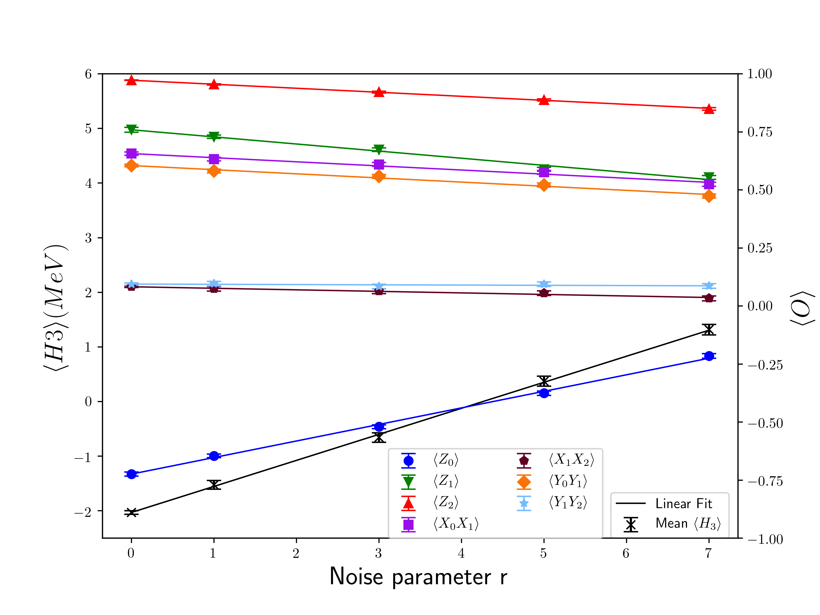
Figure 1: Expectation values of Hamiltonian terms in $H_{3}$ as a function of noise parameter $r=2M+1$. Various colored, solid symbols are the expectation values of individual terms in $H_{3}$. Black crosses are $H_{3}$, computed according to Eq. (II). Colored, solid lines are the linear fits to the corresponding individual Hamiltonian terms in $H_{3}$. The black solid line is the linear fit to $H_{3}$. We use the linear fits to extrapolate to the zero noise limit. The error bars in the figure are statistical errors based on finite sampling and a binomial distribution. The binding energy is determined as $-2.030\pm 0.034$MeV

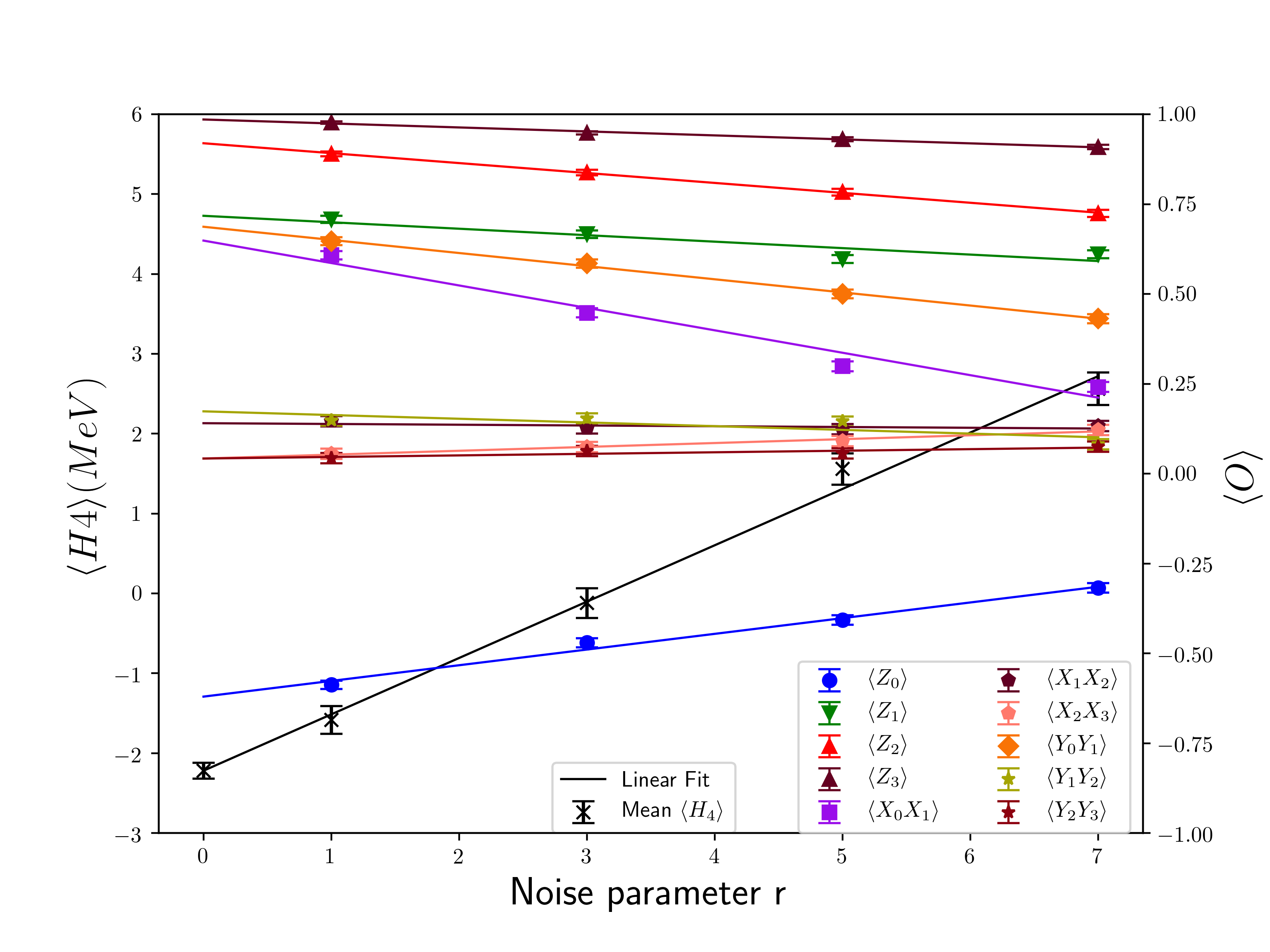
Figure 2: Expectation values of Hamiltonian terms in $H_{4}$ as a function of noise parameter $r=2M+1$. Various colored, solid symbols are the expectation values of individual terms in $H_{4}$. Black crosses are $H_{4}$, computed according to Eq. (II). Colored, solid lines are the linear fits to the corresponding individual Hamiltonian terms in $H_{4}$. The black solid line is the linear fit to $H_{4}$. We use the linear fits to extrapolate to the zero noise limit. The error bars in the figure are statistical errors based on finite sampling and a binomial distribution. The binding energy is determined as $-2.220\pm 0.179$MeV.

show in Fig. 3 the data reported in Table 1 as a visual aid. The minimal binding energy can be estimated by fitting each set of data to a quadratic form and minimizing the fit. Doing so results in individual estimates of $E_{i}=-2.080\pm-0.151$, $-2.200\pm 0.149$, $-1.946\pm 0.124$, for the three respective lambda parameters, with an average minima of $E=-2.088$ with $2.9\%$ error. Our computations therefore match previous error rates while increasing the system size, thus continuing to provide a path towards scalable simulations.

To further corroborate the accuracy of our quantum computational results, we also investigated the energy expectation values at various locations in the ansatz parameter space. Specifically, we explored the four-qubit ansatz’s parameter settings that theoretically result in approximately $10\%$ or $20\%$ deviation from the theoretical minimum by varying one parameter at a time while fixing the other two constant to their optimal values. Table 1 shows the choice of parameters and their respective, experimentally-obtained zero-noise-limit expectation values of $H_{4}$, compared with the theoretical values. We show in Fig. 3 the data reported in Table 1 as a visual aid. The minimal binding energy can be estimated by fitting each set of data to a quadratic form and minimizing the fit. Doing so results in individual estimates of $E_{i}=-2.080\pm-0.151$, $-2.200\pm 0.149$, $-1.946\pm 0.124$, for the three respective lambda parameters, with an average minima of $E=-2.088$ with $2.9\%$ error. Our computations therefore match previous error rates while increasing the system size, thus continuing to provide a path towards scalable simulations.

$\lambda_{0}$	$\lambda_{1}$	$\lambda_{2}$	$\langle H_{4}\rangle[\text{experiment}]$	$\langle H_{4}\rangle[\text{theory}]$
$0.858$	$0.958$	$0.758$	$-2.256\pm 0.179$	$-2.143$
$0.420$	$0.958$	$0.758$	$-1.568\pm 0.165$	$-1.693$
$0.550$	$0.958$	$0.758$	$-1.708\pm 0.172$	$-1.925$
$1.140$	$0.958$	$0.758$	$-1.492\pm 0.190$	$-1.921$
$1.260$	$0.958$	$0.758$	$-1.599\pm 0.191$	$-1.708$
$0.858$	$0.190$	$0.758$	$-1.425\pm 0.169$	$-1.707$
$0.858$	$0.410$	$0.758$	$-1.549\pm 0.172$	$-1.916$
$0.858$	$1.440$	$0.758$	$-2.064\pm 0.187$	$-1.915$
$0.858$	$1.630$	$0.758$	$-1.646\pm 0.188$	$-1.707$
$0.858$	$0.958$	$-0.510$	$-2.066\pm 0.179$	$-1.713$
$0.858$	$0.958$	$-0.120$	$-1.370\pm 0.182$	$-1.917$
$0.858$	$0.958$	$1.600$	$-1.524\pm 0.187$	$-1.918$
$0.858$	$0.958$	$1.930$	$-1.563\pm 0.194$	$-1.709$

Table 1: Expectation value $\langle H_{4}\rangle$ for various sets of variational parameters. $\langle H_{4}\rangle[\text{experiment}]$ denote the zero-noise limit extrapolated values of $\langle H_{4}\rangle$ obtained from our trapped-ion quantum computer. $\langle H_{4}\rangle[\text{theory}]$ denote the corresponding, theoretically predicted values. All energies are measured in MeV. The top row shows the exact minimum configuration and results. The next set of four rows show the cases where we vary $\lambda_{0}$. The following two sets of four rows show the corresponding configuration-results pair for varying $\lambda_{1}$ and $\lambda_{2}$, respectively.

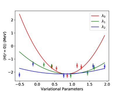
Figure 3: Expectation value $\langle H_{4}\rangle(r=0)$ as a function of a parameter chosen from the set $\{\lambda_{0},\lambda_{1},\lambda_{2}\}$. The plot symbols denote the zero-noise-limit extrapolated, also given in Table 1, and the solid lines denote the theoretical values.

IV Discussion

In this paper, we showed the quantum computational results obtained from 5- and 7-qubit trapped-ion quantum computers simulating a Deuteron. We improved on the previous result for the three-qubit ansatz and extended the ansatz size beyond the previous state of the art Dumitrescu et al. (2018). Our four-qubit ansatz result of $E_{4}=-2.220\pm 0.179$MeV may be compared with the exact Deuteron ground-state energy $-2.224$MeV.

Figure 4 shows the aggregate results, collected from previous studies performed on different quantum computing platforms on the same Deuteron system Dumitrescu et al. (2018) and our own results. For the three qubit ansatz, the error margin of the binding energy computed on the IBM QX5 was $3\%$, while it is $0.7\%$ on the IonQ-UMD trapped ion quantum computer at the optimal configuration for the three qubit experiment. Because of the demanding size of the circuit and the susceptibility of NISQ devices to errors, we were unable to run the four-qubit experiments on other quantum computing platforms. We find that, based on Fig. 4, the simulation results converge to the known ground state energy as a function of the ansatz size. We also note that, as expected, the experimental results start deviating more from the exact UCCS results, due to the accumulation of errors.

Figure 4: Aggregate results on the Deuteron simulation performed across different quantum computing platforms. Open symbols denote the experimental results. Star symbols denote the exact UCCS results. The black solid line denotes the exact deuteron ground-state energy.

Thus, we believe that our EFT simulation may be used as a practical benchmark for quantum computers which characterizes the performance of HQCC algorithms in the presence of noise, alongside the known proposals Cross et al. (2018); Benedetti et al. (2018). We have already successfully implemented the simulation across different platforms (superconducting and trapped-ion quantum computers) and also within the same platform with different configurations (5 and 7 qubit trapped-ion quantum computers). Since our ansatz circuits require only nearest-neighbor connectivity, our benchmark is expected to be readily be implemented across any platform and serve as a baseline, since more complex connectivity available on a quantum computer can only help boost the quantum computational power Linke et al. (2017). Our HQCC approach will also help benchmark the interface between quantum and classical processors. In this paper, we have taken first steps in this direction. We anticipate using the algorithm to benchmark upcoming quantum information processors.

V acknowledgments

This work is supported by the U.S. Department of Energy, Office of Science, Office of Advanced Scientific Computing Research (ASCR) Quantum Algorithm Teams and Testbed Pathfinder programs, under field work proposal numbers ERKJ332 and ERKJ335. We thank P. Lougovski and E. Dumitrescu for useful discussions. We thank T. Papenbrock for the Hamiltonian and energy extrapolation formula. Some materials presented build upon upon work supported by the U.S. Department of Energy, Office of Science, Office of Nuclear Physics under Award Nos. DEFG02-96ER40963 and DE-SC0018223 (SciDAC-4 NUCLEI). A portion of this work was performed at Oak Ridge National Laboratory, operated by UT-Battelle for the U.S. Department of Energy under Contract No. DEAC05-00OR22725.

supplementary material

V.1 Deuteron Hamiltonian

The deuteron is a shallow bound state of the proton-neutron system with a binding energy of about $B=2.2$ MeV, corresponding to a bound-state momentum $\kappa=\sqrt{2\mu B}\approx 45$ MeV ($\mu$ denotes the reduced mass). This momentum is small compared to other scales such as the pion mass at about 140 MeV, the excitation of the nucleon in a delta-resonance (at about 300 MeV), or the dividing scale $\Lambda_{\rm QCD}\approx 1$ GeV of quantum chromodynamics (QCD). The ensuing separation of scales allows us to describe the deuteron in pionless EFT Kolck (1999); Bedaque and van Kolck (2002). As the range of the nuclear interaction is small compared to the inverse bound-state momentum, any short-range central potential can be taken for a leading-order description of the deuteron in pionless EFT. For our purposes, an implementation of the effective field theory directly in the harmonic-oscillator basis Binder et al. (2016), realized as a discrete variable representation, is convenient. This also allows us to perform infrared extrapolations Furnstahl et al. (2012); Coon et al. (2012); Furnstahl et al. (2014) of results obtained in small Hilbert spaces, i.e. employing few qubits, to infinite spaces.

We consider the deuteron in its center-of-mass system. For the relative coordinate, we choose a harmonic oscillator basis with energy spacing $\hbar\omega=7$ MeV. This yields an oscillator spacing of $b=\sqrt{\hbar/(\mu\omega)}\approx 3.5$ fm. The short-ranged interaction only acts between the $0s$ state, implying an ultraviolet cutoff $\Lambda\approx\sqrt{7}/b\approx 150$ MeV König et al. (2014), and the bound-state momentum fulfills $\kappa\ll\Lambda$ as required for EFT. Thus, the cutoff is close to the breakdown scale (e.g. the pion mass) of pionless EFT.

Ideally one would pick an even larger value for $\Lambda$, either by choosing a larger oscillator spacing or by increasing the number of states where the potential is active. In our case, increasing $\hbar\omega$ further would not yield a bound state (i.e. a ground state with negative energy) when the Hilbert space is limited to a single state. Increasing the number of states where the potential is active would increase the minimum number of qubits required to perform the computation. In this work, we make effort to ensure the calculation is amenable to implementation on existing quantum computers. This motivates our current choice of parameters.

V.2 Ansatz Circuit for Trapped-Ion Quantum Computer

In order to apply the circuit that implements the ansatz state defined in Eq. (6) on a trapped-ion quantum computer, we rewrite the quantum circuit ${\mathcal{C}}_{N}$ over the native gate set amenable to implementation on a trapped-ion quantum computer. To do so, we start with useful circuit identities for those gates that appear in ${\mathcal{C}}_{N}$, decomposed into trapped-ion quantum computer native gates, as shown below.

  =    

  =    

  =    

Using the identities Maslov (2017); Maslov and Nam (2018), we obtained the ansatz-preparation circuits that are amenable to implementation on a trapped-ion quantum computer. We then optimized these circuits using known rules (see for instance Maslov and Nam (2018)), reducing the number of XX gates and RX gates, at the cost of, e.g., increasing the number of RZ gates. We chose to do so since on our quantum computer it is more costly to implement XX and RX gates than RZ gates. Figure  5 shows an exemplary case of ${\mathcal{C}}_{4}$.

Figure 5: Optimized four qubit ansatz circuit ${\mathcal{C}}_{4}$, written over a native gate set for trapped-ion quantum computers.

References

- O’Malley et al. (2016) P. J. J. O’Malley, R. Babbush, I. D. Kivlichan, J. Romero, J. R. McClean, R. Barends, J. Kelly, P. Roushan, A. Tranter, N. Ding, B. Campbell, Y. Chen, Z. Chen, B. Chiaro, A. Dunsworth, A. G. Fowler, E. Jeffrey, E. Lucero, A. Megrant, J. Y. Mutus, M. Neeley, C. Neill, C. Quintana, D. Sank, A. Vainsencher, J. Wenner, T. C. White, P. V. Coveney, P. J. Love, H. Neven, A. Aspuru-Guzik, and J. M. Martinis, Phys. Rev. X 6, 031007 (2016).
- Kandala et al. (2017) A. Kandala, A. Mezzacapo, K. Temme, M. Takita, M. Brink, J. M. Chow, and J. M. Gambetta, Nature 549, 242 (2017), arXiv:1704.05018 [quant-ph] .
- Nam et al. (2019) Y. Nam, J.-S. Chen, N. C. Pisenti, K. Wright, C. Delaney, D. Maslov, K. R. Brown, S. Allen, J. M. Amini, J. Apisdorf, et al., arXiv preprint arXiv:1902.10171 (2019).
- Benedetti et al. (2018) M. Benedetti, D. Garcia-Pintos, O. Perdomo, V. Leyton-Ortega, Y. Nam, and A. Perdomo- Ortiz, , arXiv:1801.07686 (2018).
- Temme et al. (2017) K. Temme, S. Bravyi, and J. M. Gambetta, Physical review letters 119, 180509 (2017).
- Li and Benjamin (2017) Y. Li and S. C. Benjamin, Physical Review X 7, 021050 (2017).
- Endo et al. (2018) S. Endo, S. C. Benjamin, and Y. Li, Physical Review X 8, 031027 (2018).
- McArdle et al. (2018) S. McArdle, X. Yuan, and S. Benjamin, arXiv:1807.02467 (2018).
- Jordan and Wigner (1993) P. Jordan and E. P. Wigner, in The Collected Works of Eugene Paul Wigner (Springer, 1993) pp. 109–129.
- Olmschenk et al. (2007) S. Olmschenk, K. Younge, D. Moehring, D. Matsukevich, P. Maunz, and C. Monroe, Physical Review A 76, 052314 (2007).
- Burrell (2010) A. H. Burrell, High fidelity readout of trapped ion qubits, Ph.D. thesis, University of Oxford, UK (2010).
- Landsman et al. (2018) K. A. Landsman, C. Figgatt, T. Schuster, N. M. Linke, B. Yoshida, N. Y. Yao, and C. Monroe, arXiv:1806.02807 (2018).
- Debnath et al. (2016) S. Debnath, N. M. Linke, C. Figgatt, K. A. Landsman, K. Wright, and C. Monroe, Nature 536, 63 (2016).
- Mølmer and Sørensen (1999) K. Mølmer and A. Sørensen, Physical Review Letters 82, 1835 (1999).
- Zhu et al. (2006) S.-L. Zhu, C. Monroe, and L.-M. Duan, EPL (Europhysics Letters) 73, 485 (2006).
- Choi et al. (2014) T. Choi, S. Debnath, T. Manning, C. Figgatt, Z.-X. Gong, L.-M. Duan, and C. Monroe, Physical review letters 112, 190502 (2014).
- Kim et al. (2009) K. Kim, M.-S. Chang, R. Islam, S. Korenblit, L.-M. Duan, and C. Monroe, Physical review letters 103, 120502 (2009).
- Debnath (2016) S. Debnath, A programmable five qubit quantum computer using trapped atomic ions, Ph.D. thesis (2016).
- Richardson et al. (1927) L. F. Richardson, B. J Arthur Gaunt, et al., Phil. Trans. R. Soc. Lond. A 226, 299 (1927).
- Dumitrescu et al. (2018) E. F. Dumitrescu, A. J. McCaskey, G. Hagen, G. R. Jansen, T. D. Morris, T. Papenbrock, R. C. Pooser, D. J. Dean, and P. Lougovski, Phys. Rev. Lett. 120, 210501 (2018).
- Cross et al. (2018) A. W. Cross, L. S. Bishop, S. Sheldon, P. D. Nation, and J. M. Gambetta, , arXiv:1811.12926 (2018).
- Linke et al. (2017) N. M. Linke, D. Maslov, M. Roetteler, S. Debnath, C. Figgatt, K. A. Landsman, K. Wright, and C. Monroe, Proceedings of the National Academy of Sciences 114, 3305 (2017).
- Kolck (1999) U. V. Kolck, Prog. Part. Nucl. Phys. 43, 337 (1999).
- Bedaque and van Kolck (2002) P. F. Bedaque and U. van Kolck, Annual Review of Nuclear and Particle Science 52, 339 (2002).
- Binder et al. (2016) S. Binder, A. Ekström, G. Hagen, T. Papenbrock, and K. A. Wendt, Phys. Rev. C 93, 044332 (2016).
- Furnstahl et al. (2012) R. J. Furnstahl, G. Hagen, and T. Papenbrock, Phys. Rev. C 86, 031301 (2012).
- Coon et al. (2012) S. A. Coon, M. I. Avetian, M. K. G. Kruse, U. van Kolck, P. Maris, and J. P. Vary, Phys. Rev. C 86, 054002 (2012).
- Furnstahl et al. (2014) R. J. Furnstahl, S. N. More, and T. Papenbrock, Phys. Rev. C 89, 044301 (2014).
- König et al. (2014) S. König, S. K. Bogner, R. J. Furnstahl, S. N. More, and T. Papenbrock, Phys. Rev. C 90, 064007 (2014).
- Maslov (2017) D. Maslov, New Journal of Physics 19, 023035 (2017).
- Maslov and Nam (2018) D. Maslov and Y. Nam, New Journal of Physics 20, 033018 (2018).