MFV: Application software for the visualization and characterization of the DC magnetic field distribution in circular coil systems

Abstract

The characterization of the magnetic field distribution is essential in experiments and devices that use magnetic field coil systems. We present an open-source application software, MFV (Magnetic Field Visualizer), for the visualization of the distribution of the magnetic field produced by circular coil systems. MFV models, simulates, and plots the magnetic field of coil systems composed by any number of circular coils of any size placed symmetrically along the same axis. Therefore, any new design or well known coil system, such as the Helmholtz or the Maxwell coil, can be easily modeled and simulated using MFV. A graph of the homogeneity of the magnetic field can be also produced, showing the work region where the magnetic field is homogeneous according to a percentage of homogeneity given by the user. An standardized input and output file format is employed to facilitate the exchange and archiving of data. We include some results obtained using MFV, showing its applicability to characterize the magnetic field in different coil systems. Furthermore, the magnetic field results provided by MFV were validated by comparing them with results obtained experimentally in a Helmholtz coil system.

I Introduction

The generation of homogeneous magnetic fields is required in a broad range of applications. For instance, magnetic fields are commonly used to stimulate biological systems (Malmivuo1995, ), particularly on in vitro experiments, and for the calibration of magnetic field sensors and probes (Bronaugh, ). The accuracy and reliability of the experiments developed on these kind of applications depend on different factors, but mainly on the distribution and homogeneity of the magnetic field. The most common coil system to produce homogeneous and controlled magnetic fields is the Helmholtz coil; however, its homogeneous work region is not large enough for some applications. Therefore, many efforts have been made in order to produce large homogeneous regions, and several coil systems of different sizes, shapes, and number of coils have been proposed (Gottardi2003, ; Maxwell2010, ; Merritt1983, ; Raganella1994, ; Wang2002, ; Kirschvink1992, ).

In order to employ a coil system for any kind of application that requires a work region with an homogenous magnetic flux density, it is essential to characterize the magnetic field distribution, and use this information to find the size and shape of a potential region of work where the magnetic field has a specific homogeneity value. Therefore, the development of tools to model and simulate the spatial distribution of the magnetic flux density produced by coil systems can be very useful to carry out experiments in different fields of study. For this reason, we present an open-source application software, MFV (Magnetic Field Visualizer), for the modeling, simulation, and visualization of the magnetic flux density distribution and homogeneity of circular coil systems. MFV can be used as a pedagogical tool to improve the understanding of the magnetic field distribution, or it can be used by an experimentalist to characterize the magnetic field of a coil system for an experiment or application, to design a new coil system, or to optimize experimental methodologies. Furthermore, high quality graphs of the magnetic field distribution and homogeneity can be generated using MFV.

II MFV application software

The aim of MFV is to provide the tools to easily model, simulate, and visualize the magnetic field distribution of any kind of circular coil system. The main features of MFV are the following:

• High flexibility to model and simulate a great variety of magnetic field coil systems. These systems can be composed by any number of circular coils of any size placed symmetrically along the same axis. The number of turns and the electric current through each coil can also be set by the user.

• Calculation and visualization of the magnetic flux density distribution and its homogeneity. The visualization corresponds to that of a plane parallel to the axis of symmetry of the coil system, which is enough to characterize the magnetic field distribution in all the system thanks to its rotational symmetry.

• The homogeneous work region is calculated and visualized according to a percentage of homogeneity given by the user. Parameters of a practical experimentation volume, where the magnetic field is homogeneous, are given to the user.

• A group of presets of common coils systems with pre-established parameters are provided, including the Helmholtz coil, the Maxwell coil (Maxwell2010, ), the Tetracoil (Gottardi2003, ), the Wang coil (Wang2002, ), and the Lee-Whiting coil (Kirschvink1992, ).

• The user can set different simulation parameters, including the size of the simulation region and the number of points of the simulation.

• Availability of options to make zoom and produce graphs of the magnetic field distribution and homogeneity.

• Input parameters and simulation results can be saved and loaded into the application. Furthermore, experimental results formatted accordingly can be loaded into the application to characterize the magnetic field using the available tools. The XLSX format is employed to facilitate the exchange and archiving of data.

• An estimation of the simulation time is given during the simulation.

• MFV does not require to be built in order to be executed, it is composed by executables that can be run directly on Linux 64 bits, macOS High Sierra (or later), and Windows 8 (or later) operating systems. The executables are available for download at the MFV GitHub repository (Alzate-Cardona2019, ).

II.1 Model and method

II.1.1 Magnetic field

The off-axis magnetic field (magnetic flux density) generated by a single coil placed at a point $Z$ on the axis of symmetry of the coil ($z$-axis) is given by (Smythe1939, )

$$B_{\rho}(\rho,z)=\frac{\mu_{0}}{2\pi}\frac{NI(z-Z)}{\rho[(r+\rho)^{2}+(z-Z)^{2}]^{1/2}}\times\left[\frac{r^{2}+\rho^{2}+(z-Z)^{2}}{(r-\rho)^{2}+(z-Z)^{2}}K_{2}-K_{1}\right]$$ (1)

and

$$B_{z}(\rho,z)=\frac{\mu_{0}}{2\pi}\frac{NI}{[(r+\rho)^{2}+(z-Z)^{2}]^{1/2}}\times\left[\frac{r^{2}-\rho^{2}-(z-Z)^{2}}{(r-\rho)^{2}+(z-Z)^{2}}K_{2}-K_{1}\right]\text{,}$$ (2)

where $B_{\rho}$ and $B_{z}$ are the $\rho$ and $z$ components of the magnetic field in cylindrical coordinates, respectively, $\mu_{0}$ is the vacuum permeability, $N$, $r$, and I are the number of turns, radius, and the electric current through the coil, and $K_{1}$ and $K_{2}$ are the first and second complete elliptic integrals with modulus $k$, which is given by

$$k^{2}=\frac{4r\rho}{(r+\rho)^{2}+(z-Z)^{2}}\text{.}$$ (3)

When a coil system is simulated in MFV, the contribution of each coil is calculated according to Equations 1 and 2 for all the points in the simulation region.

II.1.2 Homogeneity

The homogeneity is computed with respect to the value of the total magnetic flux density at the center of the simulation region. It is calculated as the relative difference between the value of the total magnetic field at any point ($B(\rho,z)$) and the value at the center of the simulation region ($B_{o}$), as follows

$$h=1-\frac{B(\rho,z)-B_{o}}{B_{o}}\text{.}$$ (4)

Therefore, an homogeneity of $98\%$ corresponds to a region where the values of the magnetic field do not vary more than $2\%$ from the value of reference.

II.2 Interface and usage

MFV is a very intuitive and easy-to-use application software. Several tooltips and alert messages are included in order to guide the user during the input of parameters and visualization. The interface is composed by three main sections, the input parameters window, the results window, and the zoom and homogeneity windows.

II.2.1 Input parameters

Once the MFV executable is run, the input parameters window pops up, as shown in Figure 1a. In this window, the user inputs the parameters that describe the coil system to be modeled and simulated. The menu bar located at the top of the window houses three drop-down menus. The “File” menu provides options to refresh the window (“New”), load input parameters (“Load parameters”), load simulation results (“Load results”), and quit the application (“Quit”). Input results and simulation parameters must be loaded from a file in XLSX format. The “Presets” menu contains a group of common coils systems with pre-established parameters. And the “Help” menu provides an option (“About”) to get information about the software. Below the menu bar the user can input the parameters of the coils, including the radius, number of turns, electric current, and position of the coil along the axis of symmetry ($z$-axis). Buttons to add (“+”) and remove (“-”) coils are provided. Finally, at the lower part of the window there is a button (“Simulate”) to start the simulation of the coil system. Next to the “Simulate” button there is a checkbox to decide whether to use default parameters to carry out the simulation. If the box is unchecked and the “Simulate” button is clicked, a window pops up allowing the user to set the simulation limits (in cartesian coordinates) and the number of points, as shown in Figure 1b. When the simulation is running, a small window showing the progress and remaining time of the simulation is displayed on the screen.

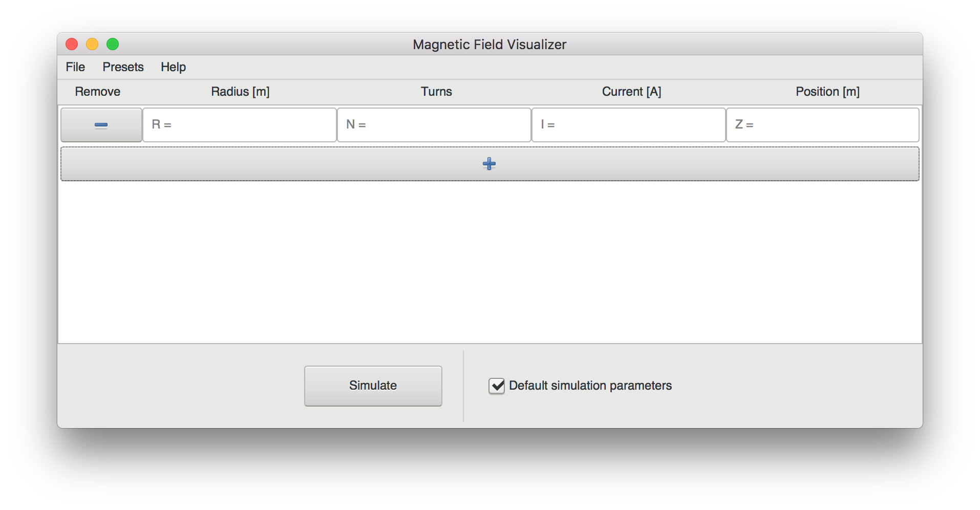
(a)

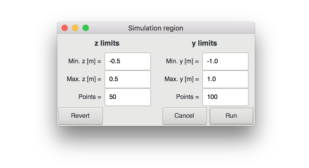
(b)

Figure 1: MFV (a) input and (b) simulation parameters windows.

II.2.2 Results

The results window shows the visualization of the magnetic flux density distribution, as shown in Figure 2. In this window, the menu bar includes the “Colormap” menu, which contains a list of different colormaps that can be used for the visualization of the magnetic field distribution. Also, the “File” menu includes an option to save (“Save as…”) the input parameters and simulation results in a XLSX file format. The main part of the results window is composed by three tabs: the first for the visualization of the magnetic field distribution (see Figure 2a), the second for the input parameters, and the third for the electric parameters (see Figure 2b) . The graph of the magnetic flux density distribution is accompanied by a color bar that indicates the values of the magnetic field in millitesla (mT). The limits of the color bar can be set by using the “Bmin” and “Bmax” entries located at the lower part of the window and clicking the “Apply” button. Three buttons are also provided to allow the user to save the graph, reset the color bar limits, and show or hide the coils in the graph. Graphs are saved in PDF format by default; however, the user can also save the them in PNG format. If the user clicks a point in the graph, a message indicating the coordinates of the point and the value of the magnetic field at that point appears in the lower part of the window, as shown in Figure 2a. The electrical parameters tab gives information about the characteristics of the wire that should be used to build the simulated coil system based on the American wire gauge (AWG).

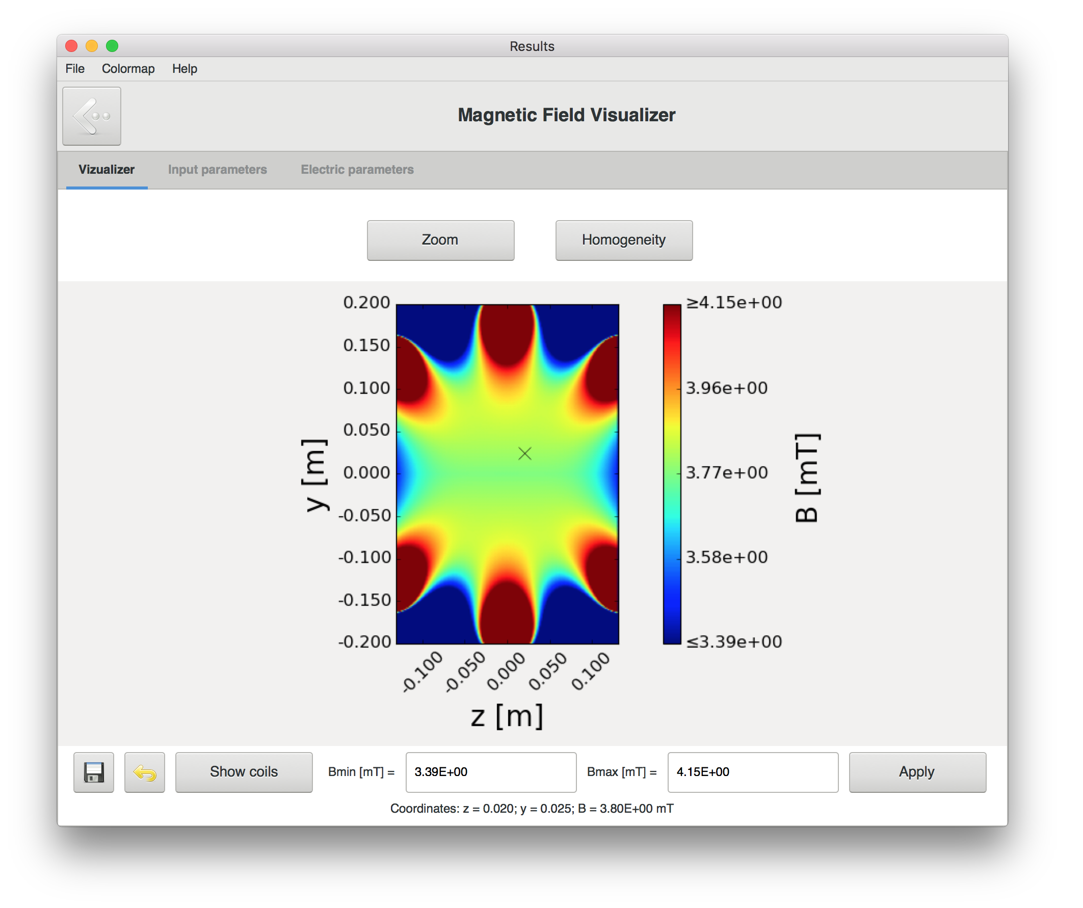
(a)

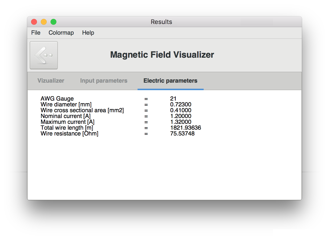
(b)

Figure 2: (a) Magnetic field distribution and (c) electrical parameters tabs of the results window. The simulated coil system corresponds to a Maxwell coil.

II.2.3 Zoom and homogeneity

The two buttons located below the tab bar in the results window, “Zoom” and “Homogeneity”, are used for the zoom and homogeneity functionalities of the software. When one of these buttons is clicked, a new window pops up. The zoom functionality allows the user to enter a zoom percentage to zoom in or zoom out the graph of the magnetic field distribution, as shown in Figure 3a. The homogeneity functionality takes as input an homogeneity percentage and plots the homogeneous region according to that percentage, as shown in Figure 3b. Because the homogeneous regions are not practical to design an experiment due to their irregular shape, the largest square that can be inscribed in the homogeneous region is computed and shown in the graph. The homogeneity window includes a tab (“Experimentation volume”) where the characteristics of a practical experimentation volume, produced due to the rotational symmetry of the circular coil systems, are provided. The practical experimentation volume corresponds to the solid of revolution generated by rotating the square region around the axis of symmetry. The size of the practical experimentation volume and its location can be useful to the user to know the best position to place a sample in an experiment. Several zoom and homogeneity windows can be opened at the same time allowing the user to compare the different graphics.

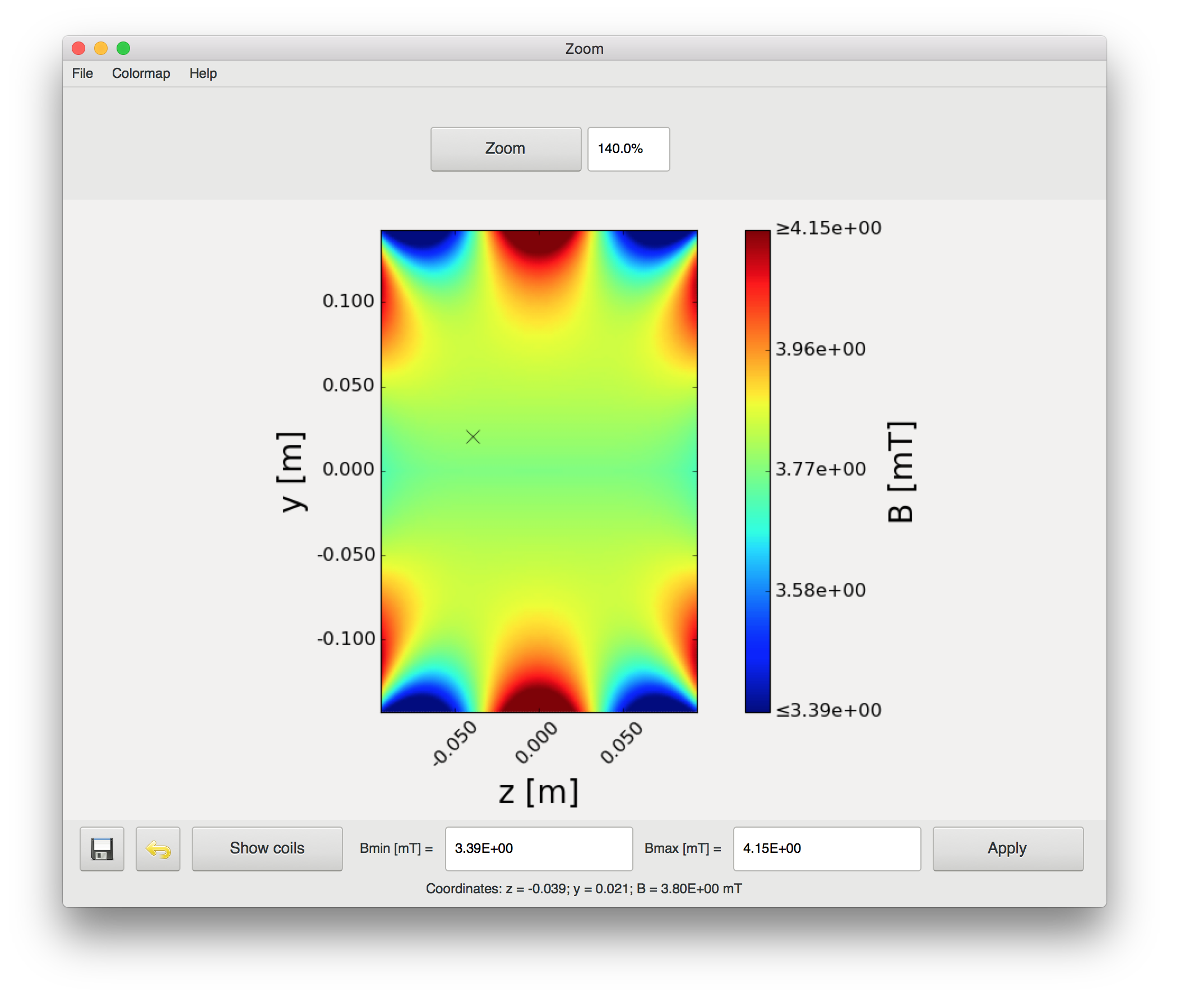
(a)

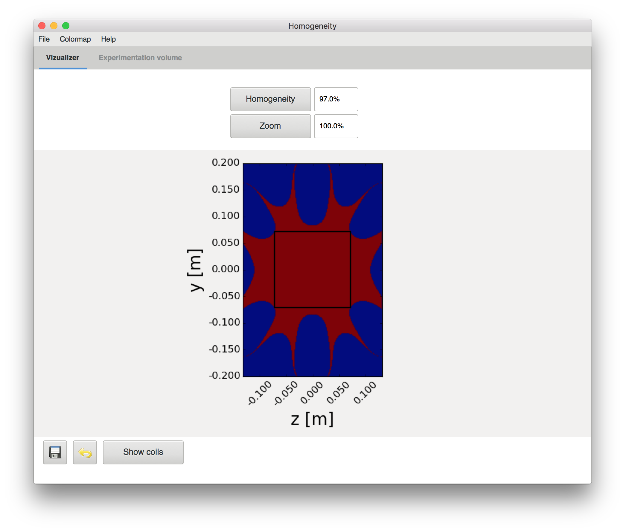
(b)

Figure 3: (a) Zoom and (c) homogeneity windows.

III Applications

In this section, we present some graphs and data obtained using MFV. Figure 4 shows graphs of the magnetic field distribution of the different presets included in the software. These graphs show how these coil systems present different magnetic field behaviors according to the number of coils, and its distribution and characteristics. Moreover, Figure 5 shows the homogeneous regions of the presets for a $97\%$ homogeneity value. These kind of results give valuable information about the coil systems, improving the understanding of the magnetic field behavior and the potential use of a given coil system for a specific application.

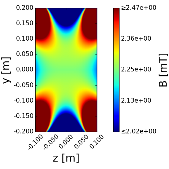
(a)

(b)

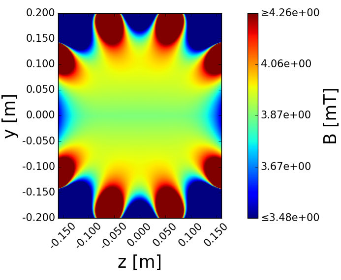
(c)

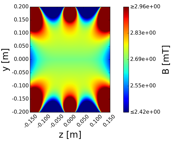
(d)

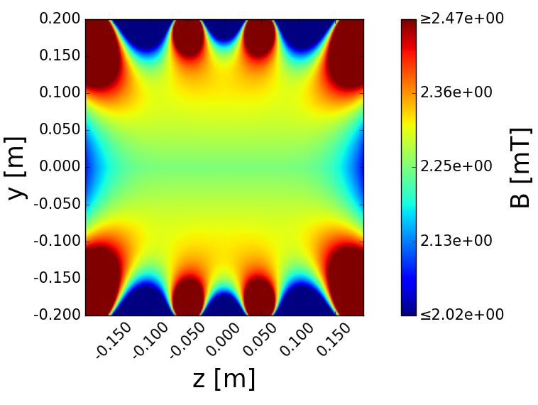
(e)

Figure 4: Magnetic field distribution of (a) Helmholtz coil, (b) Maxwell coil, (c) Tetracoil, (d) Wang coil, and (e) Lee-Whiting coil systems.

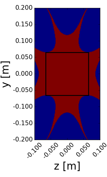
(a)

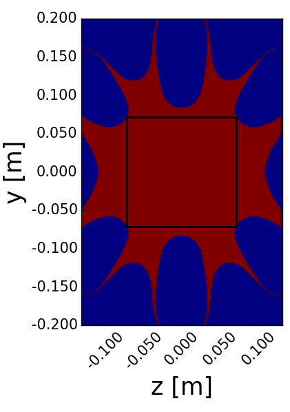
(b)

(c)

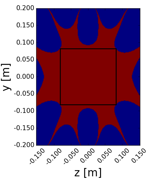
(d)

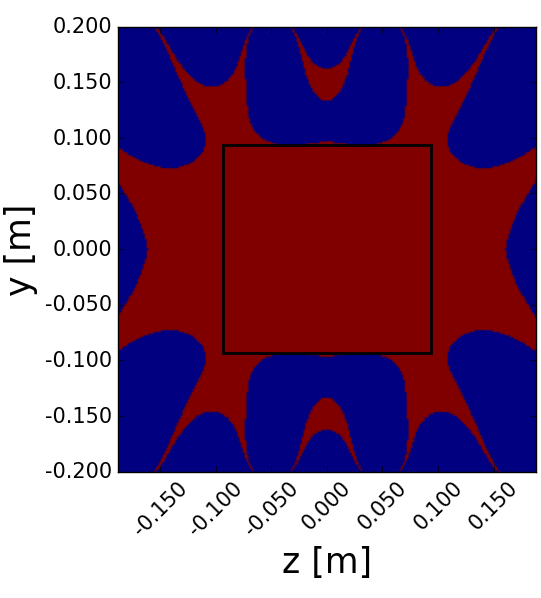
(e)

Figure 5: Homogeneous region of (a) Helmholtz coil, (b) Maxwell coil, (c) Tetracoil, (d) Wang coil, and (e) Lee-Whiting coil systems for a $97\%$ homogeneity value.

As mentioned before, the “Experimentation volume” tab in the Homogeneity window provides useful information of a potential experimentation volume. Figure 6a shows the experimentation volume parameters of the homogeneous region plotted in Figure 5a for a Helmholtz coil. Because the square region is located at the center of the Helmholtz coil and due to the rotational symmetry of the system, the experimentation volume corresponds to a cylinder. The cylinder has a height, a radius, and a volume of $0.13029\,\text{m}$, $0.06514\,\text{m}$, and $0.00174\,\text{m}^{3}$, respectively, and its centroid is located at the center of the system ($z=0.0,y=0.0$). Depending on the location of the homogeneous region with respect of the axis on symmetry, different experimentation volume shapes can be produced. The XLSX file, created when the simulation results are saved, includes the input, electrical, and simulation parameters, and the $\rho$ component, $z$ component and magnitude of the magnetic field at each point. From these results, different analysis of the magnetic field distribution can be made. For instance, from the results of the magnitude of the magnetic field of the Helmholtz coil, it is possible to plot the value of the magnetic field ($B$) along the axis of symmetry ($z$), as shown in Figure 6b. Moreover, if a new coil system design is simulated, the electrical parameters provided by the software can be helpful for the building of the coil system.

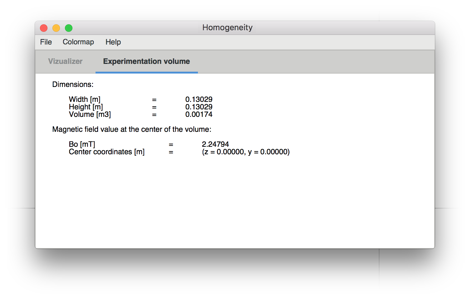
(a)

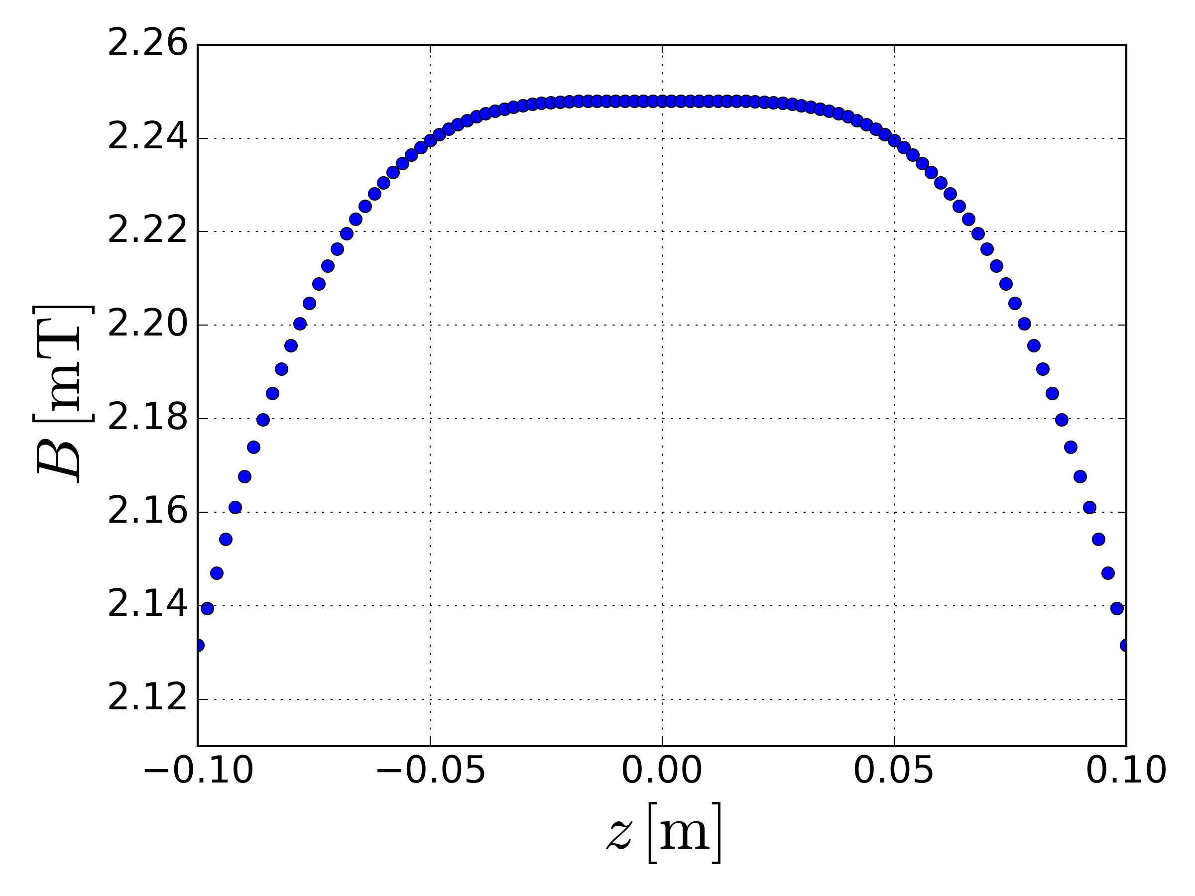
(b)

Figure 6: (a) Experimentation volume parameters and (b) magnitude of the magnetic field along the axis of symmetry of a Helmholtz coil modeled and simulated in MFV.

IV Perspectives

Different improvements are planned for MFV. Addition of new coil shapes, such as circular or rectangular shapes, would allow the modeling and simulation of other known coil systems (e.g., the Merritt coil (Merritt1983, )) and new designs that use different coil shapes. A 3D visualization of the magnetic field could be useful to give a more complete picture of the magnetic field distribution in a coil system. The practical experimentation volume can be optimized by finding the largest rectangle that can be inscribed inside the homogeneous region; however, that could require significant computational time and the implementation of an advanced algorithm. Software developers are encouraged to contribute to the development of MFV at its GitHub repository (Alzate-Cardona2019, ).

References

- (1) J. Malmivuo and R. Plonsey, Bioelectromagnetism: Principles and Applications of Bioelectric and Biomagnetic Fields. New York: Oxford University Press, oct 1995.
- (2) E. Bronaugh, “Helmholtz coils for calibration of probes and sensors: limits of magnetic field accuracy and uniformity,” in Proceedings of International Symposium on Electromagnetic Compatibility, pp. 72–76, IEEE, 1995.
- (3) G. Gottardi, P. Mesirca, C. Agostini, D. Remondini, and F. Bersani, “A four coil exposure system (tetracoil) producing a highly uniform magnetic field,” Bioelectromagnetics, vol. 24, pp. 125–133, feb 2003.
- (4) J. C. Maxwell, A Treatise on Electricity and Magnetism. Cambridge: Cambridge University Press, 2010.
- (5) R. Merritt, C. Purcell, and G. Stroink, “Uniform magnetic field produced by three, four, and five square coils,” Review of Scientific Instruments, vol. 54, pp. 879–882, jul 1983.
- (6) L. Raganella, M. Guelfi, and G. D’Inzeo, “Triaxial exposure system providing static and low-frequency magnetic fields for in vivo and in vitro biological studies,” Bioelectrochemistry and Bioenergetics, vol. 35, pp. 121–126, nov 1994.
- (7) J. Wang, S. She, and S. Zhang, “An improved Helmholtz coil and analysis of its magnetic field homogeneity,” Review of Scientific Instruments, vol. 73, pp. 2175–2179, may 2002.
- (8) J. L. Kirschvink, “Uniform magnetic fields and double-wrapped coil systems: Improved techniques for the design of bioelectromagnetic experiments,” Bioelectromagnetics, vol. 13, no. 5, pp. 401–411, 1992.
- (9) J. D. Alzate-Cardona and D. Sabogal-Suárez, “MFV,” 2019. Available at https://github.com/pcm-ca/MFV.
- (10) W. R. Smythe, Static and Dynamic Electricity. New York: McGraw-Hill, 1939.