Uphill migration in coupled driven particle systems

Abstract

In particle systems subject to a nonuniform drive, particle migration is observed from the driven to the non–driven region and vice–versa, depending on details of the hopping dynamics, leading to apparent violations of Fick’s law and of steady–state thermodynamics. We propose and discuss a very basic model in the framework of independent random walkers on a pair of rings, one of which features biased hopping rates, in which this phenomenon is observed and fully explained.

I Introduction

Particle transport in far–from–equilibrium systems often exhibits features that run counter to intuition based on equilibrium thermodynamics. One class of paradoxical behavior is that of “uphill migration,” that is, migration of particles from regions of lower to higher density in the absence of an interaction or external potential, in apparent violation of Fick’s law. Examples are found in driven lattice gases such as that studied in D14 . In this case, particles with nearest-neighbor excluded-volume interactions migrate against a density gradient, strengthening rather than reducing it, when half of the system is subject to a drive, although there is no bias in the hopping rates along the direction of the density gradient. The stationary densities in the driven and undriven cannot be predicted by equating the chemical potentials determined from the uniform systems. This is consistent with the work of Guioth and Bertin guioth2018 , who show that intensive parameters such as chemical potential can be defined if the transition rates satisfy a factorization condition. The nonuniform density profile that arises in the vicinity of the boundaries between driven and undriven regions violates this condition. While a simplistic argument in terms of effective diagonal barriers is proposed in D14 to understand uphill migration, a detailed explanation based on the exclusion interaction and hopping dynamics is lacking. Since these observations have eluded explanation, it is of interest to have simple, analytically solvable examples in which uphill migration arises. The purpose of this work is to analyze such a system.

A possible interpretation of the remarkable uphill migration phenomenon discussed above is that a particle typically spends more time in the region of higher density than in that of lower density. In this work we propose a simple model of independent random walkers on two rings, in which migration between driven and nondriven rings is observed and fully explained in terms of the typical times spent by particles in the two regions. The observed mass transport across different regions of the domain shares some interesting features with the uphill diffusion phenomenon discussed in CDMP16 ; CDMP17 ; CGGV18 in the context of lattice gas or spin models, and with particle migration on a half-driven ladder ladder07 .  

The remainder of this work is organized as follows. In Sec. II we define the model and present its stationary solution. Our analytic and simulation results are discussed in Sec. III.1, illustrating uphill migration. The connection between migration and particle sojourn times, and a connection between the latter and the gambler’s ruin problem, are analyzed in Sec. III.2. Some interesting aspects of the stationary density profiles and currents are considered in Sec. III.3, followed, in Sec. IV by a summary and discussion of our findings.

Figure 1: Schematic representation of the model.

II Model and stationary solution

We define a particle system of independent random walkers on the lattice $\Lambda=\{1,\dots,2L\}$. The lower ring consists of sites $1,...,L$ and the upper ring of sites $L+1,...,2L$, each with periodic boundaries. Mass exchange between the rings is allowed via two channels, consisting of two fixed pairs of sites: $(1,L+1)$ and $(\ell,L+\ell)$, with $2\leq\ell\leq L$ (see figure 1). The distance between channels is $\Delta=\ell-1$. The number of particles at site $i$ is denoted by $n_{i}$ and the total number of particles by $N$.

Each particle performs a random walk on the lattice with jump rate from site $i$ to site $j$ denoted by $W_{j,i}$ and defined as follows

$$W_{i\pm 1,i}=\frac{1}{2}\;\textrm{ and }\;W_{L-1,L}=W_{1,L}=\frac{1}{2}$$ (1)

for $i=2,\dots,\ell-1,\ell+1,\dots,L-1$,

$$W_{L,1}=W_{2,1}=\frac{1}{2}\;\textrm{ and }\;W_{L+1,1}=\psi$$ (2)

with $\psi\geq 0$,

$$W_{\ell\pm 1,\ell}=\frac{1}{2}\;\textrm{ and }\;W_{L+\ell,\ell}=\sigma$$ (3)

with $\sigma\geq 0$. The jump rates starting from a site in the upper ring are chosen similarly, the main difference being the presence of the drift $\varepsilon\in[0,1/2]$:

$$W_{i\pm 1,i}=\frac{1}{2}\pm\varepsilon,\,W_{2L-1,2L}=\frac{1}{2}-\varepsilon,\,W_{L+1,2L}=\frac{1}{2}+\varepsilon$$ (4)

for $i=L+2,\dots,L+\ell-1,L+\ell+1,\dots,2L-1$,

$$W_{2L,L+1}=\frac{1}{2}-\varepsilon,W_{L+2,L+1}=\frac{1}{2}+\varepsilon,W_{1,L+1}=\sigma$$

and

$$W_{L+\ell\pm 1,L+\ell}=\frac{1}{2}\pm\varepsilon\;\textrm{ and }\;W_{\ell,L+\ell}=\psi.$$

In figure 1 we show a schematic representation of the model with the particle hopping rates. The model can be recast in the the language of the zero range process EH05 with site intensity proportional to the number of particles occupying the site.

For any site $i$ we let

$$W_{i}=\sum_{j\neq i}W_{j,i}$$ (5)

be the total rate at which a particle leaves site $i$. Note that $W_{i}=1$ for any $i$, except for sites $1$, $\ell$, $L+1$, and $L+\ell$ delimiting the channels. We also let

$$W_{i,i}=-W_{i}.$$ (6)

For a given walker, let $\pi_{i}$ be the steady–state probability that it occupies site $i$. By standard results on Markov Processes, see, i.e., (Ligget, , Definition 2.3 and Exercise 2.42), we have that for any $j$

$$\sum_{i}\pi_{i}W_{j,i}=0,$$ (7)

which can be rewritten as

$$\pi_{j}=\sum_{i\neq j}\pi_{i}\frac{W_{j,i}}{W_{j}}.$$ (8)

Exploiting independence, in the stationary state the mean number of particles at the generic site $i$ is

$$\rho_{i}=N\pi_{i}.$$ (9)

The main quantities of interest in this note are the lower and upper density profiles $\rho_{i}$ with $i=1,\dots,L$ and $i=L+1,\dots,2L$, respectively, and the average mass displacement between the lower and the upper rings,

$$\chi=\frac{1}{N}\Big{[}\sum_{i=1}^{L}\rho_{i}-\sum_{i=L+1}^{2L}\rho_{i}\Big{]}=\frac{1}{N}\sum_{i=1}^{L}(\rho_{i}-\rho_{L+i}).$$ (10)

Figure 2: Points: simulation results for mass displacement $\chi$ vs $\sigma/\psi$ for $\psi=0.1$ (triangles), $\psi=1$ (squares), and $\psi=10$ (circles), with $L=50$, $\Delta=25$, $N=200$, $\varepsilon=0.1$ (solid symbols), and $\varepsilon=0$ (open symbols). Solid lines denote the exact solution.

III Results

In this paper we focus on the behavior of the profiles $\rho_{i}$ and the mass displacement $\chi$ as a function of the model parameters. For given parameters, we obtain the exact value by first solving equations (8) to compute the $\pi_{i}$’s, and then equation (9) and (10). In the simulations, the total number of particles is $N=200$ and $L=50$.

III.1 Mass displacement: uphill currents

In this section our principal focus is on the behavior of $\chi$ as a function of the model parameters. Figs. 2–4 compare exact results for $\chi$ with those of Monte Carlo simulations.

In figure 2 the mass displacement $\chi$ is plotted as a function of the ratio $\psi/\sigma$ for different choices of the other parameters. For zero drift, the model is symmetric for any choice of parameters and the mass displacement $\chi$ vanishes. For $\varepsilon>0$, mass migration is observed ($\chi\neq 0$), except for the symmetric case, $\sigma/\psi=1$. Moreover, in the symmetric case $\sigma/\psi=1$, for any $\varepsilon\geq 0$, the upper and lower profiles $\rho_{i}$ are uniform, independent of $i$. The result for $\psi=\sigma$ is expected: in this case symmetry is ensured by the fact that in a state in which the mean number of particles is the same at each site, the rates at which particles move upward and downward are equal in each channel.

For various choices of the parameters we find $\chi>0$, namely, we observe mass migration towards the non–driven, lower ring. This phenomenon is not trivial, since the model is designed in such a way that upward and downward rates in the two channels should compensate each other even when $\psi\neq\sigma$.

Figure 3: Simulation results for $\chi$ vs $\varepsilon$ for $\Delta=1$ (triangles), $\Delta=25$ (squares), and $\Delta=L-1$ (circles), with $L=50$, $\sigma=10$, $\psi=1$, and $N=200$. Solid lines denote the exact solution.

Figure 4: $\chi$ vs $\Delta$ for $\varepsilon=0.01$ (triangles), $\varepsilon=0.05$ (squares), and $\varepsilon=0.1$ (circles); other parameters as in figure 3. Solid lines denote the exact solution.

In Figs. 3 and 4 the mass displacement is plotted as a function of the drift $\varepsilon$ and the intra–channel distance $\Delta$, respectively. These graphs show that both positive and negative mass displacements are possible. More precisely, given $\varepsilon$ not too large, if the intra–channel distance $\Delta$ is small enough then the mass displacement is negative, i.e., the mass in the driven ring is larger than that in the non–driven one. The fact that mass migration is observed in both directions is similar to the phenomenon described in D14 , although in that work it is connected to the possible jumps that particles may perform, whereas here it depends on simple geometric features.

Figure 5: Simulation results for the ratio of the average sojourn times in the upper and in the lower ring of a single target particle as a function of $\varepsilon$, for $\Delta=1$ (triangles), $\Delta=25$ (squares), and $\Delta=49$ (circles), with $L=50$, $N=200$, $\sigma=10$ and $\psi=1$ (solid symbols), $\sigma=10^{3}$ and $\psi=0$ (open symbols). The solid lines are computed using the gambler’s ruin expressions for $\tau_{\textrm{up}}$ and $\tau_{\textrm{down}}$.

III.2 Sojourn times and gambler’s ruin

Mass migration can be interpreted in terms of the average residence times, called upper and lower sojourn time and denoted respectively by $\tau_{\textrm{up}}$ and $\tau_{\textrm{down}}$, that a particle spends in the upper and in the lower ring. These times can be defined by attaching a label to each particle $i$, and following its position over time. Then $\tau_{\textrm{up}}$ is defined as the mean time (over the evolution and over particles) between entering and exiting the upper ring, in the stationary state; $\tau_{\textrm{down}}$ is defined analogously. Sojourn times are similar to the residence times that have been widely studied for the simple exclusion process CKMSpre2016 and for the simple symmetric random walk CCSpre2018 . The main difference is that in those studies the geometry of the strip was considered and the residence time was defined conditioning the particle to exit the strip through the side opposite the one where it started the walk.

The idea is very simple: if the upper sojourn time is larger than the lower one, then particles will spend more time in the upper ring and, at stationarity, a negative mass displacement will be observed. This idea is confirmed by the simulation results plotted in figure 5, where the ratio of the upper and the lower sojourn times is plotted as a function of the drift. Indeed, comparing data in figure 5 to those in figure 3, a perfect mirror behavior is seen, i.e., $\tau_{\textrm{up}}>\tau_{\textrm{down}}$ corresponds to $\chi<0$ and vice-versa. Note, in particular, that the curves for $\Delta=25$ and $\Delta=49$ intersect at the same value of the drift $\varepsilon$ in both graphs.

The interpretation in terms of sojourn times also provides a nice explanation of the dependence of the sign of $\chi$ on the inter–channel distance. In Figs. 3–5 we consider $\sigma=10\gg(1/2\pm\varepsilon)$ and $\psi=1\approx(1/2\pm\varepsilon)$. Under this assumption particles typically jump from the upper ring to the lower one at site $L+1$, and from the lower one to the upper one at site $\ell$.

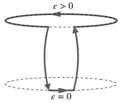
Figure 6: Typical path covered by a particle in the limiting case with $\sigma\gg\psi$ and $\Delta$ small.

Figure 7: Stationary density profiles for $\sigma=10$ and $\psi=1$, with $L=50$, $\Delta=L/2$, and drift $\varepsilon=0$ (which corresponds to $\chi=0$), $0.05$ (center, with $\chi=0.2874$), $0.3$ (right, with $\chi=0.5768$). Empty and solid symbols denote, respectively, the density profiles in the upper and the lower rings. Solid lines denote the exact solution.

Figure 8: Stationary density profiles for $\sigma=10$ and $\psi=1$, with $L=50$, $\Delta=5$, and, from the left to the right, drift $\varepsilon=0$ (which corresponds to $\chi=0$), $0.05$ (with $\chi=-0.0929$), $0.0897$ (with $\chi=0.0002$), and $0.3$ (with $\chi=0.3145$). Empty and solid symbols denote, respectively, the density profiles in the upper and the lower rings. Solid lines denote the exact solution.

Hence, the upper sojourn time is quite close to the typical time that a particle needs to move from site $L+\ell$ to site $L+1$ along the upper ring, whereas the lower sojourn time is quite close to the typical time that a particle needs to move from site $1$ to site $\ell$ along the lower ring. In view of this remark, due to the presence of the drift, the upper sojourn time is, for most choices of the parameters, smaller than the lower one, explaining why, in general the mass migration is observed towards the lower, non–driven ring. The contrary is observed when $\Delta$ is small. Indeed, in this case the lower sojourn time is substantially smaller than the upper one. Although no drift is present, the lower sojourn time is smaller than the upper one because the distance to be covered is much smaller than in the upper, driven ring, cf. figure 6.

This latter observation suggests a way of estimating the sojourn times that should be quite accurate for $\sigma\gg 1\gg\psi$. Indeed, in this case one can use a classic result of probability theory, namely, the gambler’s ruin estimate of the duration of the game, see (Feller1968, , Chapter XIV, Section 3) and CCpreprint2018 , to obtain

$$\tau_{\textrm{down}}\simeq(\ell-1)(L-\ell+1)$$ (11)

and

$$\tau_{\textrm{up}}\simeq\frac{\ell-1}{1-2\Big{(}\frac{1}{2}+\varepsilon\Big{)}}-\frac{L}{1-2\Big{(}\frac{1}{2}+\varepsilon\Big{)}}\frac{1-\Big{(}\frac{\frac{1}{2}-\varepsilon}{\frac{1}{2}+\varepsilon}\Big{)}^{\ell-1}}{1-\Big{(}\frac{\frac{1}{2}-\varepsilon}{\frac{1}{2}+\varepsilon}\Big{)}^{L-1}}.$$ (12)

The ratio $\tau_{\textrm{up}}/\tau_{\textrm{down}}$ computed using the above expressions is plotted in figure 5, where, as expected, the agreement is poor for $\sigma=10$ and $\psi=1$, while it is strikingly perfect for $\sigma=10^{3}$ and $\psi=0$. Indeed, in such an extreme case, particles move along the two rings closely following the gambler’s ruin rules. The sole difference with respect to the gambler’s ruin problem is in the tiny probability $1-\sigma/(1+\sigma)$ that a particle at site $L+1$ does not jump to the site $1$ and a particle at the site $\ell$ does not jump to $L+\ell$.

III.3 Density profiles and steady–state currents

This section is devoted to a brief discussion of the typical stationary particle density profiles, which depend on both the drift $\varepsilon$ and on the ratio $\sigma/\psi$. As explained above, we perform a series of MC simulations to investigate the stationary density profiles in the two rings. The initial datum, in our simulations, is represented by uniform density profiles, with the same number of particles shared by the two rings. The numerical results are then compared to the exact ones obtained as explained at the beginning of Section III.

We have already mentioned that in the symmetric case $\sigma/\psi=1$, for any $\varepsilon\geq 0$, the upper and lower profiles $\rho_{i}$ are uniform, namely they do not depend on the site $i$, and $\chi=0$. This is expected since, in such a case, in a state in which the average number of particles is the same at each site, the rates at which particles move upward and downward are equal in each channel.

Setting $\psi\neq\sigma$ yields nonuniform stationary profiles in the two rings. In particular, figure 7, for $\varepsilon=0$, shows the onset of piecewise linear density profiles (i.e., stationary solutions to the discrete Laplace equation) in both rings, with kinks at the locations of the two channels. For reasons of symmetry, there is no net mass transfer between the rings, hence we again have $\chi=0$.

The center and the left panel in figure 7 show how the profile shape is modified when the drift in the upper channel is different from zero, which is the paradigmatic case that leads to “uphill currents”, namely states with $\chi\neq 0$. We notice, indeed, that, since $\chi>0$ holds in the cases shown in the figure, the overall mass residing in the upper ring, in the stationary state, is less than that in the lower ring. Moreover, it also worth noting that the profiles are not linear in the upper ring due to the presence of the drift.

The plots in figure 8 refer to an inter–channel distance $\Delta=5$, small enough to produce a non–monotonic behavior of $\chi$ as a function of $\varepsilon$, already highlighted in figure 3 for $\Delta=1$. In particular, for small values of the drift, particles gather on the upper ring ($\chi<0$), whereas for larger values of the drift they tend to move downwards to the lower ring ($\chi>0$).

We have also learned that in our model there are two classes of stationary states showing no uphill diffusion, as also visible in figure 2. The first class is obtained by setting $\psi=\sigma$ and/or $\varepsilon=0$: in particular, the case with $\psi=\sigma$ and $\varepsilon=0$ corresponds to a state with vanishing current and whose density profiles are uniform (except for the coupling sites) over the two rings. The second class includes the states for which the (moderate) effect of the drift in the upper ring is exactly compensated by the (small) inter–channel distance covered by particles in the lower ring, see the third panel from the left in figure 8. These are nonequilibrium steady states characterized by nonuniform density profiles and nonvanishing currents, which nevertheless produce no net mass transfer between the rings.

Figure 9: Steady state currents $J^{\textrm{u}}_{\Delta}$ (empty circles), $J^{\textrm{u}}_{L-\Delta}$ (empty squares), $J^{\textrm{d}}_{\Delta}$ (solid circles), $J^{\textrm{d}}_{L-\Delta}$ (solid squares), $J^{\textrm{c}}_{1}$ (empty triangles), and $J^{\textrm{c}}_{\ell}$ (empty diamonds) as function of the drift $\varepsilon$, for $\sigma=10$, $\psi=1$, with $L=50$, $\Delta=5$ (left panel) and $\Delta=L/2$ (right panel). Solid lines denote the exact solution.

We conclude this subsection discussing the behavior of the stationary currents. As remarked in Section I, the transient to the stationary state is characterized by uphill currents flowing against the direction predicted by Fick’s law. On the other hand, as we show here, the steady–state currents flow as predicted by the Fick’s law.

The steady–state current $J_{i\to j}$ from site $i$ to site $j$ is defined as the mean value, with respect to the stationary measure, of the quantity $n_{i}W_{j,i}-n_{j}W_{i,j}$ Due to the structure of the jump rates $W_{j,i}$, the current $J_{i\to j}$ is nonzero only for neighboring sites $i$ and $j$ in the rings and along the channels connecting the two rings. Averaging with respect to the stationary measure and recalling Eq. (9) we have,

$$J_{i\to j}=\rho_{i}W_{j,i}-\rho_{j}W_{i,j}=N(\pi_{i}W_{j,i}-\pi_{j}W_{i,j}).$$ (13)

Thus, at stationarity, we consider the following six currents: $J^{\textrm{u}}_{\Delta}=J_{L+\ell-1\to L+\ell}$ flows in the branch of the upper ring of length $\Delta$; $J^{\textrm{u}}_{L-\Delta}=J_{L+\ell\to L+\ell+1}$ flows in the branch of the upper ring of length $L-\Delta$ from site $L+\ell$ to site $L+1$; $J^{\textrm{d}}_{\Delta}=J_{\ell-1\to\ell}$ flows in the branch of the lower ring of length $\Delta$ from site $\ell$ to site $1$; $J^{\textrm{d}}_{L-\Delta}=J_{\ell\to\ell+1}$ flows in the branch of the lower ring of length $L-\Delta$ from site $\ell$ to site $1$; $J^{\textrm{c}}_{1}=J_{L+1\to 1}$ flows in the channel from site $L+1$ to site $1$; and $J^{\textrm{c}}_{\ell}=J_{L+\ell\to\ell}$ flows in the channel from site $L+\ell$ to site $\ell$. Note that currents within the rings are conventionally taken as positive when particles move counterclockwise on the ring, i.e., from a site $x$ to neighbor site $y>x$ (recall that periodic boundary conditions are imposed), whereas currents between the rings are taken as positive when flowing from the upper to the lower ring.

The behavior of these currents as functions of the drift $\varepsilon$ is shown in Figure 9: on the left we consider a case with small $\Delta$ and on the right the case $\Delta=L/2$. Further details are given in the caption. We first note that, at stationarity, the currents in the channels are nonzero, but since they are opposed (empty triangle and empty diamonds), the total current between the two rings is zero. Another interesting remark is that in the driven ring, the currents are approximately proportional to the drift $\varepsilon$, whereas in the symmetric ring the current is nonzero, due to the drift in the upper ring, but approaches a constant value as $\varepsilon$ is increased. Finally, it is easy to check that the sign of the currents in the undriven ring is consistent with Fick’s law when compared with the density profiles plotted in Figures 7 and 8.

III.4 Transient uphill currents

As a final remark, we observe that the presence of uphill currents is highlighted by considering the transient behavior of the total current flowing between the rings as time goes by. By the expression total particle current at time $t$ we refer to the difference between the total number of particles which jumped from the upper to the lower ring and those which jumped in the opposite direction in the interval from zero to $t$, divided by $t$. (Recall that migration is considered positive when downward). In the left panel of Figure 10 the total current flowing in the channels is shown as a function of time in a particular realization of the process for various inter-channel distances $\Delta$. The right panel (with logaritmic horizontal scale), for the same realization of the process, shows the mass displacement $\chi$ as a function of time.

Note that for a moderate drift $\varepsilon=0.05$ and a small distance $\Delta=5$ (filled diamonds) the current is negative, consistent with the negative average mass displacement $\chi$ shown in the right panel. The case $\Delta=25$ can be understood similarly. Note in figure 10, that when time becomes large, the system attains a steady state in which the total current exchanged between the rings vanishes tends to zero. Figure 9 reveals, in particular, that at stationarity $J^{\textrm{c}}_{1}$ is precisely the opposite of $J^{\textrm{c}}_{\ell}$, for any value of the drift $\varepsilon$.

Figure 10: Left: Total current flowing between rings (left), and mass displacement $\chi$ (right), versus time for $\sigma=10$ and $\psi=1$, with $L=50$, $\epsilon=0.05$, and, from the left to the right, $\Delta=5$ (solid diamonds), $\Delta=15$ (empty circles), $\Delta=25$ (empty triangles), $\Delta=35$ (empty squares). (See the text for further details.) Dashed lines are a guide for the eye. On the right, for legibility we plot results for only two values of $\Delta$.

IV Conclusions

We consider a simple, exactly solvable model of noninteracting particles exhibiting migration despite overall symmetry. The model consists of independent random walkers hopping on and between a pair of rings, with particle exchange between rings allowed at specified channels. The combination of asymmetry between the channels and a drift in one (but not both) rings leads to particle migration between rings, as shown by the exact solution of the model and confirmed in Monte Carlo simulations. In the limit of strong channel asymmetry, particle migration can be understood on the basis of the classic gambler’s ruin problem.

Our results show that “uphill migration”, in apparent violation of Fick’s law, may be significantly more general than has been appreciated until now, in that it does not depend on inter–particle interactions. A promising arena for observation of this phenomenon is the movement of passive tracers in cyclic geophysical flows.

- (1) R. Dickman, Failure of steady–state thermodynamics in nonuniform driven lattice gases, 2014, Phys. Rev. E 90, 062123.
- (2) J. Guioth and E. Bertin, Large deviations and chemical potential in bulk–driven systems in contact, 2018, Europhys. Lett. 123, 10002.
- (3) M. Colangeli, A. De Masi, E. Presutti, Latent heat and the Fourier law, 2016, Phys. Lett. A 380, 1710–1713.
- (4) M. Colangeli, A. De Masi, E. Presutti, Particle models with self sustained current, 2017, J. Stat. Phys. 167, 1081–1111.
- (5) M. Colangeli, C. Giardinà, C. Giberti, C. Vernia, Nonequilibrium two-dimensional Ising model with stationary uphill diffusion, 2018, Phys. Rev. E 97, 030103(R).
- (6) R. Dickman and R. R. Vidigal, Particle redistribution and slow decay of correlations in hard–core fluids on a half-driven ladder, 2007, J. Stat. Mech. P05003.
- (7) M.R. Evans, T. Hanney, Nonequilibrium statistical mechanics of the zero–range process and related models, 2005, J. Phys. A: Math. Gen. 38, R195.
- (8) T.H. Ligget, Continuous Time Markov Processes, An Introduction, Graduate Studies in Mathematics, vol. 113, American Mathematical Society, Providence, Rhode Island, 2010.
- (9) E.N.M. Cirillo, M. Colangeli, Stationary uphill currents in locally perturbed zero–range processes, 2017, Phys. Rev. E 96, 052137.
- (10) E.N.M. Cirillo, O. Krehel, A. Muntean, and R. van Santen, Lattice model of reduced jamming by a barrier, 2016, Phys. Rev. E 94, 042115.
- (11) A. Ciallella, E.N.M. Cirillo, J. Sohier. Residence time of symmetric random walkers in a strip with large reflective obstacles, 2018, Physical Review E 97, 052116.
- (12) W. Feller. An Introduction to Probability Theory and its Applications, volume 1. John wiley & Sons, Inc, New York – London – Sidney, 1968.
- (13) A. Ciallella and E.N.M. Cirillo, Conditional expectation of the duration of the classical gambler problem with defects, in press on Eur. Phys. J. Spec. Top..