Imperial/TP/2019/JG/01
Toric geometry and the dual of -extremization
Jerome P. Gauntletta, Dario Martellib,† 22footnotetext: On leave at the Galileo Galilei Institute, Largo Enrico Fermi, 2, 50125 Firenze, Italy.and James Sparksc
aBlackett Laboratory, Imperial College,
Prince Consort Rd., London, SW7 2AZ, U.K.
bDepartment of Mathematics, King’s College London,
The Strand, London, WC2R 2LS, U.K.
Mathematical Institute, University of Oxford,
Andrew Wiles Building, Radcliffe Observatory Quarter,
Woodstock Road, Oxford, OX2 6GG, U.K.
We consider , gauge theories arising on membranes sitting at the apex of an arbitrary toric Calabi-Yau 4-fold cone singularity that are then further compactified on a Riemann surface, , with a topological twist that preserves two supersymmetries. If the theories flow to a superconformal quantum mechanics in the infrared, then they have a supergravity dual of the form AdS, with electric four-form flux and where is topologically a fibration of a Sasakian over . These solutions are also expected to arise as the near horizon limit of magnetically charged black holes in AdS, with a Sasaki-Einstein metric on . We show that an off-shell entropy function for the dual AdS2 solutions may be computed using the toric data and Kähler class parameters of the Calabi-Yau 4-fold, that are encoded in a master volume, as well as a set of integers that determine the fibration of over and a Kähler class parameter for . We also discuss the class of supersymmetric AdS solutions of type IIB supergravity with five-form flux only in the case that is toric, and show how the off-shell central charge of the dual field theory can be obtained from the toric data. We illustrate with several examples, finding agreement both with explicit supergravity solutions as well as with some known field theory results concerning -extremization.
1 Introduction
A common feature of supersymmetric conformal field theories (SCFTs) with an abelian R-symmetry is that the R-symmetry, and hence important physical observables, can be obtained, in rather general circumstances and in various spacetime dimensions, via an extremization principle. In SCFTs in , for example, the R-symmetry can be obtained via the procedure of -maximization [2], while for SCFTs in it can be obtained via -extremization [3]. In each of these cases one constructs a trial central charge, determined by the ’t Hooft anomalies of the theory, which is a function of the possible candidate R-symmetries. After extremizing the trial central charge one obtains the R-symmetry, and when the trial central charge is evaluated at the extremal point one gets the exact central charge and the right moving central charge, , for the and SCFTs, respectively.
Next, for SCFTs in , one can use -extremization [4]. The key quantity now is the free energy of the theory defined on a round three sphere, . After extremizing a trial , again calculated as a function of the possible R-symmetries, one finds both the R-symmetry and the free energy at the extremal point. Turning to SCFTs in with two supercharges and an abelian R symmetry, there is not, as far as we know, an analogous general field theory proposal concerning -extremization, although one has been recently discussed in the context of holography [5], as we recall below. On the other hand there is a proposed “-extremization” procedure [6] for the class of such SCFTs that arise after compactifying an SCFT in on a Riemann surface, , of genus111The genus case was discussed in [6]; generalizing to was discussed in [7] and noted in footnote 5 of [8], building on [1, 9]. . For this class one considers the topologically twisted index for the theory on as a function of the twist parameters and chemical potentials for the flavour symmetries. After extremization one obtains the index, which is expected to be the same as the logarithm of the partition function of the SCFT. While significant evidence for -extremization has been obtained, it does not yet have the same status as the -, - and - extremization principles.
For the special subclass of these SCFTs that also have a large holographic dual, we can investigate the various extremization principles from a geometric point of view. To do this one first needs to find a precise way of taking the supergravity solutions off-shell in order to set up an appropriate extremization problem. A guiding principle, that has been effectively utilised in several different situations, is to identify a suitable class of supersymmetric geometries in which one demands the existence of certain types of Killing spinors, but without imposing the full equations of motion. The best understood examples are those associated with Sasaki-Einstein () geometry, specifically the class of AdS solutions of type IIB and the AdS solutions of supergravity that are dual to SCFTs in and SCFTs in , respectively. Here one goes off-shell by relaxing the Einstein condition and considering the space of Sasaki metrics. It was shown in [10, 11] that the Reeb Killing vector field for the Sasaki-Einstein metric, dual to the R-symmetry in the field theory, can be obtained by extremizing the normalized volume of the Sasaki geometry as a function of the possible Reeb vector fields on the Sasaki geometry. Interestingly, while this geometric extremization problem is essentially the same for and , and indeed is applicable for arbitrary , it is associated with the different physical phenomena of -maximization and -extremization in the and dual field theories, respectively (although see [12]).
In a recent paper [5] an analogous story was presented for the class of AdS solutions of type IIB with non-vanishing five-form flux only [13] and the class of AdS solutions of supergravity with purely electric four-form flux [14], that are dual to SCFTs in and SCFTs in , respectively. The geometry associated with these solutions was clarified in [15] where it was also shown that they are examples of an infinite family of “GK geometries” . As explained in [5], one can take these GK geometries off-shell in such a way to obtain a class of supersymmetric geometries for which, importantly, one can still impose appropriate flux quantization conditions. These supersymmetric geometries have an R-symmetry vector which foliates the geometry with a transverse Kähler metric. Furthermore, a supersymmetric action can be constructed which is a function of the R-symmetry vector on as well as the basic cohomology class of the transverse Kähler form. Extremizing this supersymmetric action over the space of possible R-symmetry vectors, for the case of , then gives the R-symmetry vector of the dual SCFT as well as the central charge, after a suitable normalization. For the case of , it was similarly shown that the on-shell supersymmetric action, again suitably normalized, corresponds to the logarithm of the partition function of the dual SCFT. This is the holographic version of an -extremization principle for such SCFTs that we mentioned above, whose field theory formulation remains to be uncovered.
In [16] we further developed this formalism for the class of AdS solutions in which arises as a fibration of a toric over . From a dual point of view such solutions can arise by starting with a quiver gauge theory dual to AdS, with a Sasaki-Einstein metric on , and then compactifying on with a topological twist. Using the toric data of , succinct formulas were presented for how to implement the geometric version of -extremization for the dual SCFT. A key technical step was to derive a master volume formula for toric as a function of an R-symmetry vector and an arbitrary transverse Kähler class. Based on various examples, it was conjectured in [16] that there is an off-shell agreement between the geometric and field theory versions of -extremization and this was then proven for the case of toric in [17].
In this paper, we extend the results of [16] in two main ways. First, we generalise the formalism to the class of AdS solutions where itself is toric. This requires generalizing the master volume formula for toric that was presented in [16] to toric . These results provide a general framework for implementing the geometric dual of -extremization that applies to , SCFTs that do not have any obvious connection with a compactification of a , SCFT dual to AdS. In a certain sense these results provide an AdS analogue of the results on AdS solutions, with toric [10]. As an illustration, we use the formalism to re-derive the central charge of some known explicit AdS solutions constructed in [18], just using the toric data.
Second, we consider AdS solutions where arises as fibration of a toric over , which allows us to make contact with -extremization. These solutions can be obtained by starting with an , SCFT dual to an AdS solution of supergravity, with a Sasaki-Einstein metric on , and then compactifying on with a topological twist to ensure that two supercharges are preserved. Using the master volume formula on we can generalise the results of [16] to derive formulae which provide a geometric dual of -extremization.
The principle of -extremization, introduced in [6], arose from the programme of trying to reproduce the Bekenstein-Hawking entropy of supersymmetric black holes by carrying out computations in a dual field theory. Indeed this was achieved for a class of AdS4 black holes with AdS horizons in the context of the ABJM theory in [6], and some interesting extensions have appeared in [8, 19, 20, 21, 22, 23, 24], for example. It is natural to expect that many and perhaps all of the AdS solutions that we consider here, with a fibration of a toric over , can arise as the near horizon limit of supersymmetric black holes. Such black holes, with horizon, would asymptote to AdS in the UV, with the conformal boundary having an factor associated with the field theory directions, and approach the AdS solutions in the IR. We will therefore refer to the suitably normalized supersymmetric action for this class of as the entropy function since, as argued in [5], it will precisely give the black hole entropy after extremization.
Now for a general class of quiver gauge theories, using localization techniques it was shown that the large limit of the topological index can be expressed in terms of a Bethe potential [1]. Furthermore, it was also shown in [1] that the same Bethe potential gives rise to the free energy of the SCFT on the three sphere, . Combining these field theory results with the geometric results of this paper then provides a microscopic derivation of the black hole entropy for each such black hole solution that actually exists. This provides a rich framework for extending the foundational example studied in [6] associated with and the ABJM theory.
An important general point to emphasize is that, as in [5, 16], the geometric extremization techniques that we discuss in this paper will give the correct quantities in the dual field theory, provided that the AdS3 and AdS2 and solutions actually exist. In other words they will give the correct results provided that there are no obstructions to finding a solution. A related discussion of obstructions to the existence of Sasaki-Einstein metrics can be found in [25] and furthermore, for toric Sasaki-Einstein metrics it is known that, in fact, there are no such obstructions [26]. No general results are yet available for AdS and AdS solutions, although several examples in which the existence of the supergravity solution is obstructed were discussed in [5, 16], showing that this topic is an important one for further study.
The plan of the rest of the paper is as follows. In section 2 we consider toric, complex cone geometries, , in four complex dimensions. In the special case that the metric on the cone is Kähler then the metric on is a toric Sasakian metric. Using the toric data we derive a master volume formula for as a function of an R-symmetry vector and an arbitrary transverse Kähler class, generalising a similar analysis for cone geometries in three complex dimensions carried out in section 3 of [16]. In section 3 we deploy these results to obtain expressions for the geometric dual of -extremization for AdS geometries when is toric and study some examples.
In section 4 we analyse AdS solutions when is a fibration of a toric over a Riemann surface , generalising the analysis in section 4 of [16]. We illustrate the formalism for the universal twist solutions of [27], in which one fibres a manifold over , with , in which the fibration is just in the R-symmetry direction of and in addition the fluxes are all proportional to the R-charges, recovering some results presented in [8]. We also consider some additional generalizations for the special cases when and for which we can compare results obtained using our new formulae with some explicit supergravity solutions first constructed in [28]. We then consider an example in which is the product of the conifold with the complex plane. Some new features arise for this example, as the link, , of this cone contains worse-than-orbifold singularities and some care is required in using the master volume formulae. For this example, we are able to make a match between the off-shell entropy function and the twisted topological index calculated from the field theory side in [29] in the genus zero case. We then revisit the case of and are able to match the off-shell entropy function with the twisted topological index calculated from the field theory side, which was calculated in [29] in the genus zero case. Following this, we consider another example, with similar singularities, associated with being a certain Calabi-Yau 4-fold singularity, that is closely related to the suspended pinch point 3-fold singularity. Once again we can match with some field theory results of [1]. We end section 4 with some general results connecting our formalism with the index theorem of [1]. We conclude with some discussion in section 5.
In appendix A we have included a few details of how to explicitly calculate the master volume formula from the toric data in the specific examples discussed in the paper, while appendix B contains a derivation of a homology relation used in the main text. Appendix C analyses flux quantization for the AdS2 solutions of [28] that we discuss in section 4.
Note added: as this work was being finalised we became aware that there would be significant overlap with the results of [30], which appeared on the arXiv on the same day.
2 Toric geometry and the master volume formula
2.1 General setting
We will be interested in complex cones, , in complex dimension that are Gorenstein, i.e. they admit a global holomorphic -form . Furthermore, we demand that there is an Hermitian metric that takes the standard conical form
| (2.1) |
where the link (or cross-section) of the cone, , is a seven-dimensional manifold. The complex structure pairs the radial vector with a canonically defined vector . Likewise, the complex structure pairs with the dual one-form , and . The vector has unit norm and defines a foliation of . The basic cohomology for this foliation is denoted .
For the class of geometries of interest [5], we furthermore require the vector to be a Killing vector for the metric on , with
| (2.2) |
where the metric transverse to the foliation is conformally Kähler, with Kähler two-form .
Finally, in this paper we will also take the metric to be invariant under a isometry, with the isometry generated by being a subgroup. Introducing generators , , for each action, where has period , we may then parametrize the vector in terms of , with
| (2.3) |
For convenience, we choose a basis so that the holomorphic -form has unit charge under and is uncharged under , . Notice that we then have222For the case of geometry we need to take , as discussed below. For the supersymmetric AdS3 geometry discussed in section 3 we take , while for the supersymmetric AdS2 geometry discussed in section 4 we need .
| (2.4) |
This also implies that
| (2.5) |
where denotes the Ricci two-form of the transverse Kähler metric, and moreover , where is the basic first Chern class of the foliation.
2.2 Toric Kähler cones
We now assume that the cone metric is Kähler so that the metric on is a toric Sasakian metric, as studied in [10]. In this case the transverse conformally Kähler metric in (2.2) is Kähler. Denoting the transverse Kähler form by , we have
| (2.6) |
Because is also a transverse symplectic form in this case, by definition is a contact one-form on and , satisfying and , is then called the Reeb vector field.
Considering now the isometries, we may define the moment map coordinates
| (2.7) |
These span the so-called moment map polyhedral cone , where are standard coordinates on . The polyhedral cone , which is convex, may be written as
| (2.8) |
where are the inward pointing primitive normals to the facets, and the index labels the facets. Furthermore, , where , follows from the Gorenstein condition, in the basis for described at the end of the previous subsection. An alternative presentation of the polyhedral cone is
| (2.9) |
where are the outward pointing vectors along each edge of .
As shown in [10], for such a Kähler cone metric on the R-symmetry vector necessarily lies in the interior of the Reeb cone, . Here the Reeb cone is by definition the dual cone to . In particular is equivalent to for all edges . Using , together with (2.3) and (2.7), the image of under the moment map is hence the compact, convex three-dimensional polytope
| (2.10) |
where the Reeb hyperplane is by definition
| (2.11) |
Later we will frequently refer to the toric diagram (in a minimal presentation) which is obtained by projecting onto the vertices , with the minimum set of lines drawn between the vertices to give a convex polytope. When all of the faces of the toric diagram are triangles the link of the toric Kähler cone is either regular or has orbifold singularities. We will also discuss cases in which some of the faces of the diagram are not triangles and then there are worse-than-orbifold singularities (for some further discussion see [31]).
2.3 Varying the transverse Kähler class
As in [16], we first fix a choice of toric Kähler cone metric on the complex cone . This allows us to introduce the moment maps in (2.7), together with the angular coordinates , , as coordinates on . Geometrically, then fibres over the polyhedral cone : over the interior of this is a trivial fibration, with the normal vectors to each bounding facet in specifying which collapses along that facet.
For a fixed choice of such complex cone, with Reeb vector given by (2.3), we would then like to study a more general class of transversely Kähler metrics of the form (2.2). In particular, we would like to compute the “master volume” given by
| (2.12) |
as a function both of the vector , and transverse Kähler class . With the topological condition , discussed in [5], which will in fact hold for all the solutions considered in this paper, all closed two-form classes on can be represented by basic closed two-forms. Following [16], if we take the to be basic representatives in that lift to integral classes in , which are Poincaré dual to the restriction of the toric divisors on , then we can write
| (2.13) |
Furthermore, the are not all independent and will depend on just of the parameters . As in [5] it will also be useful to note that the first Chern class of the foliation can be written in terms of the as
| (2.14) |
In the special case in which
| (2.15) |
we recover the Sasakian Kähler class and the master volume (2.12) reduces to the Sasakian volume
| (2.16) |
Following [16], this volume can be shown to be
| (2.17) |
Here the factor of arises by integrating over the torus , while is the Euclidean volume of the compact, convex three-dimensional polytope
| (2.18) |
Here
| (2.19) |
which lies in the interior of , while the parameters determine the transverse Kähler class. It will be important to remember that the transverse Kähler class , and hence volume , depends on only of the parameters , with three linear combinations being redundant.
We may compute the Euclidean volume of in (2.18) by first finding its vertices . By construction, these arise as the intersection of an edge of with the Reeb hyperplane . Let us fix a specific two-dimensional facet of , associated with a specific , given by
| (2.20) |
This is a compact, convex two-dimensional polytope, and will have some number of edges/vertices. In turn, each edge of arises as the intersection of with other faces which we label , each associated with , with . We choose the ordering of cyclically around the th face and it is then convenient to take the index numbering on to be understood mod (hence cyclically). The vertices of arise from the intersection of neighbouring edges in this ordering. We may thus define the vertex of as the intersection
| (2.21) |
where , with the index numbering on understood mod (hence cyclically). By definition, then satisfies the four equations
| (2.22) |
which we can solve to give
| (2.23) |
Here denotes a determinant, and we have defined
| (2.24) |
Here and, to be clear, the vector index on the left hand side of (2.23) corresponds to the vector index on on the right hand side.
We next divide up into tetrahedra, as follows. For each face , , we first split the face into triangles. Here the triangles have vertices , where . Each of these triangles then forms a tetrahedron by adding the interior vertex . The volume of is then simply the sum of the volumes of all of these tetrahedra. On the other hand, the volume of the tetrahedron with vertices is given by the elementary formula
| (2.25) |
Thus, the master volume (2.17) can now be written as
| (2.26) |
On the other hand, using the explicit formula (2.23) for the vertices , together with some elementary identities, we find the master volume formula for is given by
where we have defined
| (2.28) |
Notice that is cubic in the , as it should be. When all of the are equal, , , using a vector product identity these simplify considerably to give
| (2.29) |
In particular, for the special case of the Sasakian Kähler class with , as in (2.15), the formula (2.3) reproduces the known [32] expression for the volume of toric Sasakian manifolds, namely
| (2.30) |
In [10] it was shown that the Reeb vector for a Sasaki-Einstein metric on is the unique minimum of on , considered as a function of , subject to the constraint .
It will be helpful to present some formulas here that will be useful later. Using (2.13) the master volume may be written as
| (2.31) |
where the triple intersections are defined as
| (2.32) |
We then have
| (2.33) |
Furthermore, the first derivative of the master volume with respect to gives the volume of the torus-invariant five-manifolds , Poincaré dual to the , via
| (2.34) |
Finally, we note that the Sasakian volume and the Sasakian volume of torus-invariant five-dimensional submanifolds , , can be expressed in terms of the as
| (2.35) |
For the various examples of that we consider later which are regular or have orbifold singularities, we have explicitly checked that the relation
| (2.36) |
holds as an identity for all and . We have not yet constructed a proof of this result, but we conjecture that it will always hold for this class of . When it does hold it is simple to see that the master volume formula is invariant under the “gauge” transformations
| (2.37) |
for arbitrary constants , generalising a result of [17]. Noting that the transformation parametrized by is trivial, this explicitly shows that the master volume only depends on of the parameters , as noted above.
However, we emphasize that (2.36) does not hold for which have worse-than-orbifold singularities, unless we impose some additional restrictions on the . This is an important point since many examples whose field theories have been studied in the literature have this property. We discuss this further for the representative example of the link associated with the product of the complex plane with the conifold in appendix A.3.
To conclude this section we note that the above formulae assume that the polyhedral cone is convex, since at the outset we started with a cone that admits a toric Kähler cone metric. However, as first noted in [33], and discussed in [5, 16], this convexity condition is, in general, too restrictive for applications to the classes of AdS2 and AdS3 solutions of interest. Indeed, many such explicit supergravity solutions are associated with “non-convex toric cones”, as defined in [5], which in particular have toric data which do not define a convex polyhedral cone. We conjecture that the key formulae in this section are also applicable to non-convex toric cones and we will assume that this is the case in the sequel. The consistent picture that emerges, combined with similar results in [5, 16], strongly supports the validity of this conjecture.
3 Supersymmetric AdS solutions
3.1 General set-up
In this section the class of supersymmetric AdS solutions of type IIB supergravity that are dual to SCFTs with supersymmetry of the form
| (3.1) |
Here is an overall dimensionful length scale, with being the metric on a unit radius AdS3 with corresponding volume form . The warp factor is a function on the smooth, compact Riemannian internal space and is a closed two-form on with Hodge dual . In order to define a consistent string theory background we must impose the flux quantization condition
| (3.2) |
which also fixes . Here denotes the string length, is the string coupling constant, and , with forming an integral basis for the free part of . The geometry of these solutions was first analysed in [13] and then extended in [15].
The geometric dual to -extremization, described in detail in [5], starts by considering supersymmetric geometries. By definition these are configurations as in (3.1) which admit the required Killing spinors. These off-shell supersymmetric geometries become supersymmetric solutions when, in addition, we impose the equation of motion for the five-form. Equivalently, we obtain supersymmetric solutions when the equations of motion obtained from extremizing an action, , given explicitly in [15] are satisfied.
The supersymmetric geometries have the properties stated at the beginning of section 2.1. In particular, we have
| (3.3) |
where is a transverse Kähler metric with transverse Kähler form . This is exactly as in (2.2) after making the identification . The transverse Kähler metric determines the full supersymmetric geometry, including the fluxes. In particular, the conformal factor is fixed via where is the Ricci scalar of the transverse Kähler metric. We also have
| (3.4) |
where is the Ricci two-form of the transverse Kähler metric, and , with . The Killing vector is called the R-symmetry vector.
Putting the supersymmetric geometries on-shell implies solving the equations of motion coming from varying a supersymmetric action, , which is the action mentioned above evaluated on a supersymmetric geometry. Explicitly it was shown in [5] that
| (3.5) |
which, in fact, just depends on the R-symmetry vector and the transverse Kähler class i.e. . Furthermore, in order to impose flux quantization on the five-form the following topological constraint must also be imposed
| (3.6) |
Flux quantization is achieved by taking a basis of 5-cycles, , that are tangent to and demanding
| (3.7) |
with .
Assuming now that is toric, admitting a isometry as discussed in section 2.1, it is straightforward to generalize section 3 of [16] to obtain expressions for , the constraint and the flux quantization conditions in terms of the toric data. Remarkably, they can all be expressed in terms of the master volume given in (2.3). Specifically, using the formulas given in section 2.3, the off-shell supersymmetric action, the constraint equation and the flux-quantization conditions are given by
| (3.8) | ||||
| (3.9) | ||||
| (3.10) |
respectively, where . The are not all independent: they are the quantized fluxes through a basis of toric five-cycles . While the generate the free part of , they also satisfy 4 linear relations , and hence we have
| (3.11) |
Notice that the component of this relation is in fact the constraint equation (3.9).
We also note that when (2.36) holds, from the invariance of the master volume under the transformations (2.37) it follows that all the derivatives of with respect to are also invariant. Therefore, the complete set of equations (3.8), (3.9), (3.10) is invariant under (2.37) and we could use this to “gauge-fix” three of the parameters, or alternatively work with gauge invariant combinations. However, in the examples below we will not do this, but instead we will see that the results are consistent with the gauge invariance. Finally, we also note that we can also write the supersymmetric action in the form
| (3.12) |
where we used the fact the master volume is homogeneous of degree three in the (see (2.31)).
We can now state the geometric dual to -extremization of [5], for toric . We hold fixed to be , and then extremize with respect to as well as the independent Kähler class parameters determined by , subject to the constraint (3.9) and flux quantization conditions (3.10). Equivalently, we extremize the “trial central charge”, , defined by
| (3.13) |
which has the property that for an on-shell supersymmetric solution, i.e. after extremization, we obtain the central charge of the dual SCFT:
| (3.14) |
In practice, and generically, we have independent flux quantum numbers that we are free to specify. The constraint equation and of the flux quantization conditions (3.10) can be used to solve for the independent . This leaves as a function of the independent flux numbers as well as , of which we still need to vary the latter. We emphasize that (3.14) will be the central charge of the CFT dual to the AdS solution, provided that the latter actually exists (i.e. when there are no obstructions).
We now illustrate the formalism by considering a class of explicit AdS supergravity solutions presented333The local solutions were constructed as a special example of a class of AdS3 solutions of supergravity found in [28]. in [18]. The construction involves a four-dimensional Kähler-Einstein () base manifold with positive curvature, . Such manifolds are either , or a del Pezzo surface with . Of these , and are toric. The solutions depend on two integers with , and we will label them . The associated complex cones over are non-convex toric cones, as defined in [5, 16], and the associated compact polytopes are not convex.
The exposition in [27] illuminated the very close similarity of these solutions with a class of seven-dimensional Sasaki-Einstein manifolds, , constructed in [34], which utilized exactly the same manifolds. For the latter, using techniques developed in [35], the toric geometry of the associated Calabi-Yau 4-fold singularities for and was discussed in [31]. The integers are both positive and satisfy , with for and for . The associated compact polytopes for these ranges are, of course, convex. Below we shall analyse these two families in turn. Although we will not utilize this below, we note that both of these examples satisfy the relation (2.36) for the master volume.
3.2 The and families
The toric data associated with was given in [31], in the context of the discussion of explicit Sasaki-Einstein metrics. We take the inward pointing normal vectors to be given by
| (3.15) |
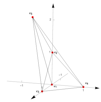
The associated toric diagram, obtained by projecting on the vertices in (3.2), is given in Figure 1. For we have , and we have a convex polytope. However, for the explicit solutions we have and . We continue with general .
The master volume given in (2.3) can be obtained from the toric data (3.2) and some results in appendix A. In the Sasakian limit, , setting and extremizing with respect to [10] we find that the critical Reeb vector is given by , with solving the cubic equation
| (3.16) |
The fact that is due to the symmetry of the base space. Equivalently, the value of obtained from (3.16) can be obtained from extremizing the Sasakian volume with upon setting , which reads
| (3.17) |
This expression, with obtained from (3.16), can be shown to be precisely equal to the Sasaki-Einstein volume
| (3.18) |
given in equation (2.13) of [31], where it was computed using the explicit Sasaki-Einstein metric. The relation between the variables and in the two expressions above is simply . Note, for example, for the special case , we have and .
We now turn to the AdS solutions. We begin by setting in the formulae (3.9)–(3.10). The transverse Kähler class is determined by of the parameters . We use the constraint equation (3.9) and one of the flux equations (3.10), which we take to be , to solve for two of the which we take to be and . The remaining fluxes can all be expressed in terms of , and the flux vector is given by
| (3.19) |
We can then calculate the trial central charge finding, in particular, that it is independent of , and , in agreement with the invariance of the problem under the three independent transformations in (2.37). Furthermore, is quadratic in and , again as expected. It is now straightforward to extremize with respect to these remaining variables and we find the unique extremum has , with
| (3.20) |
The fact that is again due the symmetry of the base space. Evaluating at this extremum we find the central charge is given by
| (3.21) |
This is the central charge for the AdS solutions, provided that they exist. We can now compare with the explicit solutions constructed in [18]. These solutions depended on two relatively prime integers (which were labelled in [18]). We first note that in [18] we should set , , and since we are considering . We then need to make the identifications
| (3.22) |
The flux vector is then . In particular, we identify , with , in equation (18) of [18], respectively, while are associated with . With these identifications, we precisely recover the result for the central charge given in equation (1) of [18]. Note that the conditions , required to have an explicit supergravity solution [18], translate into the conditions
| (3.23) |
as mentioned earlier. In particular the polytope is not convex, as observed in [33].
It is an interesting outstanding problem to identify the SCFTs that are dual to these AdS solutions.
3.3 The and families
The toric data associated with was given in [31]. We take the inward pointing normal vectors to be given by
| (3.24) |
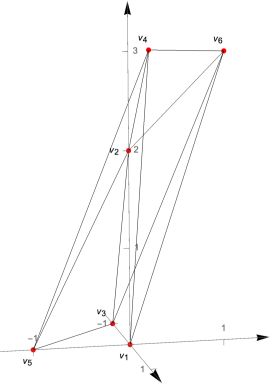
The associated toric diagram, obtained by projecting on the vertices in (3.3), is given in Figure 2. For we have , and there is a convex polytope. For the explicit metrics we again have and . We continue with general .
The master volume , given in (2.3), can be obtained from the toric data (3.3) and the results in appendix A. In the Sasakian limit, , setting and extremizing with respect to [10] we find that the critical Reeb vector is given by , with solving the cubic equation
| (3.25) |
The fact that is due to the symmetry of the base space. Equivalently, the value of obtained from (3.25) can be obtained from extremizing the Sasakian volume with upon setting , which reads
| (3.26) |
Again, this expression, with obtained from (3.25), can be shown to be precisely equal to the Sasaki-Einstein volume
| (3.27) |
given in equation (2.13) of [31], where it was computed using the explicit Sasaki-Einstein metric. The relation between the variables and in the two expressions above is . Note, for example, for the special case we have and .
We now turn to the AdS solutions. We begin by setting in the formulae (3.9)–(3.10). The transverse Kähler class is determined by of the parameters . We use the constraint equation (3.9) and two of the flux equations (3.10), which we take to be and , to solve for three of the which we take to be , and . The remaining fluxes are then expressed in terms of , , and we have
| (3.28) |
It will be useful in a moment to notice that if we restrict the fluxes by imposing , then .
We next calculate the trial central charge and find, in particular, that it is independent of , and , in agreement with the invariance of the problem under the three independent transformations in (2.37). Furthermore, is quadratic in and , again as expected. It is now straightforward to extremize with respect to these remaining variables and we find the unique extremum has , with
| (3.29) |
The fact that is due to the symmetry of the base space. Evaluating at this extremum we find the central charge is given by
| (3.30) |
This is the central charge for the AdS solutions, provided that they exist. We can now compare the above results, for the special case that the fluxes are restricted via as mentioned above, with the explicit solutions constructed in [18]. These solutions depended on two relatively prime integers (which were labelled in [18]). Since we are considering , we need to set and in the formulae in [18]. We also need to make the identifications
| (3.31) |
The flux vector is then . In particular, we identify , with , in equation (18) of [18], respectively, while are associated with . With these identifications, we precisely recover the result for the central charge given in equation (1) of [18]. The analysis of [18] shows that the supergravity solutions exist for , which translates into the conditions
| (3.32) |
In particular the polytope is not convex, as observed in [33].
It is interesting that the central charge for these AdS can also be obtained in another way. Indeed, by selecting one of the factors, we can view as a fibration of over the other factor, as discussed in section 6.1 and 7.2 of [16] (and we note that were denoted in [16]). The fibration in [16] was specified by three integers , with , as demanded by supersymmetry, and for simplicity and were taken to be equal with . In addition, the solutions were specified by an additional two integers, , which determined the fluxes. To compare to the solutions discussed here we should first restrict the solutions so that the fibration has . We then need to make the identifications as well as . Having done this, one finds that the central charge in (3.30) agrees exactly with equation (6.7) of [16].
It is an interesting outstanding problem to identify the SCFTs that are dual to these explicit AdS solutions. In particular, as discussed in [16], viewing them as a fibration of over we have and hence they are not associated, at least in any simple way, with compactifying the quiver gauge theories dual to AdS, with Sasaki-Einstein metric on , since the latter have .
Finally, we note that the explicit supergravity solutions in [18] with can be generalised, allowing the relative sizes of the two to be different. Indeed such local solutions can be obtained by T-dualising the solutions in section 5 of [27]. It is natural to conjecture that regular solutions with properly quantized flux can be obtained with independent , , and central charge as in (3.30).
4 Supersymmetric AdS solutions
4.1 General set-up
We now consider supersymmetric AdS solutions of supergravity that are dual to superconformal quantum mechanics with two supercharges of the form
| (4.1) |
Here is an overall length scale and is the metric on a unit radius AdS2 with volume form . The warp factor is a function on the compact Riemannian internal space and is a closed two-form on . We also need to impose flux quantization. Since for the above ansatz, we need to impose
| (4.2) |
where is the Planck length and , with forming an integral basis for the free part of . The geometry of these solutions was first analysed in [14] and then extended in [15].
We again consider off-shell supersymmetric geometries, as described in detail in [5]. These are configurations of the form (4.1) which admit the required Killing spinors and become supersymmetric solutions when we further impose the equation of motion for the four-form. The complex cone , in complex dimension and with Hermitian metric , admits a global holomorphic -form . The complex structure pairs the radial vector with the R-symmetry vector field . Likewise, the complex structure pairs with the dual one-form , and . The vector has unit norm and defines a foliation of . The basic cohomology for this foliation is denoted .
The supersymmetric geometries have a metric of the form
| (4.3) |
where is a transverse Kähler metric with transverse Kähler form . The transverse Kähler metric determines the full supersymmetric geometry including the fluxes. In particular, the conformal factor is fixed via , where is the Ricci scalar of the transverse Kähler metric. We also have
| (4.4) |
where is the Ricci two-form of the transverse Kähler metric, and , with . It was shown in [5] that there is a supersymmetric action , whose extremum allows one to determine the effective two-dimensional Newton’s constant, , with giving the logarithm of the partition function of the dual superconformal quantum mechanics.
In this paper we are interested in the specific class of which are fibred over a Riemann surface :
| (4.5) |
The R-symmetry vector is assumed to be tangent to . While the general class of supersymmetric AdS solutions might arise as the near horizon limits of black hole solutions of supergravity, this seems particularly likely in the case that is of the fibred form (4.5). Indeed we expect that such solutions can arise as the near horizon limit of black holes, with horizon topology , in an asymptotically AdS background with a Sasaki-Einstein metric on . In fact this is known to be the case for the so-called universal twist fibration with genus [36, 37, 38, 27, 39]. As shown in [5] the entropy of the black holes, , should be related to the effective two-dimensional Newton’s constant, , via . In the following we will refer to the supersymmetric action , with a suitable normalization given below, as the entropy function.
We now further consider to be toric with an isometric action, as described in section 2. In order to obtain , we can generalise the analysis of section 4 of [16]. The fibration structure is specified by four integers and we have
| (4.6) |
since we have chosen a basis for the vectors satisfying (2.4) with . Furthermore, up to an irrelevant exact basic two-form, the transverse Kähler form on may be taken to be
| (4.7) |
Here is a Kähler form on the complex cone over that is suitably twisted over . We have normalized , and is effectively a Kähler class parameter for the Riemann surface.
By directly generalizing the arguments in section 4.2 of [16], we find that the key quantities can all be expressed in terms of and as well as the master volume . The supersymmetric action is given by
| (4.8) |
The constraint equation that must be imposed, in order that flux quantization is well-defined, is given by
| (4.9) |
Finally, we consider flux quantization, and there are two types of seven-cycle to consider. First, there is a distinguished seven-cycle, , which is a copy of obtained by picking a point on , and we have
| (4.10) |
We can also consider the seven-cycles , , obtained by fibreing a toric five-cycle on , over , and we have
| (4.11) |
We find it convenient to also introduce the equivalent notation for the fluxes :
| (4.12) |
The toric five-cycles are not all independent. The generate the free part of , but they also satisfy 4 linear relations . This gives rise to the corresponding homology relation in , , which implies the useful relation444A topological proof of (4.13) may be found in appendix B. It would be nice to prove this relation more directly, using a similar method to that given in (4.37)–(4.39) of [16].
| (4.13) |
We thus have a total of independent flux numbers and . In all of the above formulae we should set
| (4.14) |
after taking any derivatives with respect to the . Finally, we note that we can also express the supersymmetric action in the following compact form
| (4.15) |
To prove this we first multiply (4.11) by and then sum over . Recalling that the master volume is homogeneous of degree three in the and using Euler’s theorem we deduce that
| (4.16) |
For a given fibration, specified by with , the on-shell action is obtained by extremizing . A priori with , there are parameters comprising , along with the independent Kähler class parameters and . The procedure is to impose (4.9), (4.10) and (4.11), which, as we noted, is generically independent conditions, and hence will generically be a function of three remaining variables. We then extremize the action with respect to these variables, or equivalently extremize the “trial entropy function”, , defined by
| (4.17) |
which has the property that for an on-shell supersymmetric solution, i.e. after extremization, we obtain the two-dimensional Newton’s constant
| (4.18) |
As explained in [5] this should determine the logarithm of the partition function of the dual supersymmetric quantum mechanics. Moreover, when the AdS solution arises as the near horizon limit of a black hole solution, it gives the entropy of the black hole, . The entropy of such black holes should be accounted for by the microstates of the dual , field theories when placed on ; the number of these microstates is expected to be captured by the corresponding supersymmetric topological twisted index.
We may also compute the geometric R-charges associated with the operators dual to M5-branes wrapping the toric divisors at a fixed point on the base . The natural expression555We have not verified this formula by explicitly checking the -symmetry of an M5-brane wrapped on the toric divisors . It is analogous to the corresponding expression for AdS3 solutions, where it was also motivated by computing the dimension of baryonic operators dual to D3-branes wrapping supersymmetric cycles in [40]. We will indirectly verify this normalization below. is given by
| (4.19) |
Following similar arguments to those of section 4 in [16] we then deduce that
| (4.20) |
As for the fluxes in (4.12), we find it convenient to strip out a factor of and define
| (4.21) |
In particular, using (4.10), notice that we have
| (4.22) |
We also note that for the generic examples, with toric data satisfying (2.36) we have, equivalently,
| (4.23) |
from which the relation (4.22) is the component. Recall that this relation implies that the master volume is invariant under the “gauge transformation” (2.37) acting on the . As we noted in the previous section, this implies that all of the derivatives of with respect to are also invariant under this gauge transformation. However, this is not the case after taking derivatives with respect to (since the gauge transformation involves the vector ) and so we now discuss the effect of (2.37) on the extremal problem in the case of fibered geometries666This analysis applies also to the geometries discussed in [16]..
The variation of under (2.37) is given by
| (4.24) |
On the other hand, assuming that (2.36) holds and taking a derivative of this with respect to , a short computation leads to the identity [16]
| (4.25) |
and hence we have
| (4.26) |
where we used (4.10). A similar computation for the variation , and using the expression obtained by differentiating (4.25) with respect to , we deduce that
| (4.27) |
Using these results we find that if we extend the gauge transformation to also allow for a variation of the Kähler class parameter via
| (4.28) |
where the second expression in the second line follows from (4.13), then in addition to being invariant then so are the fluxes as well as the supersymmetric action , as one can easily see from the expression (4.15).
While these gauge transformations are certainly interesting and useful, they are constrained. This follows from the fact that since and parametrize Kähler classes they must satisfy some positivity constraints. For example, the transformations (4.1) naively suggest that we might choose a gauge with , but this should not be possible. In fact in some of the examples we study, one finds , on-shell, which also indicates the problem with such a putative gauge choice. It would certainly be interesting to determine the positivity constraints on the Kähler class parameters and hence the restrictions on the gauge transformations.
4.2 Entropy function in terms of variables
Before discussing some explicit examples of AdS solutions with obtained as a fibration of toric over , we first show that the above variational problem incorporates some general features concerning -extremization discussed in [1]. We will further develop the connection of our formalism to -extremization, in the subsequent subsections, especially section 4.8.
The master volume is defined to be a function of independent variables . We want to consider a change of variables in which is, instead, a function of the variables (see (4.21)) given by
| (4.29) |
where at this stage is a free parameter (i.e. not yet given by (4.10) so we don’t yet impose .) Assuming that this is an invertible change of variables, using the chain rule, we then have
| (4.30) |
Using this, and also (4.10), we can then write the supersymmetric action (4.8) as
| (4.31) |
We next multiply the expression for the fluxes , given in (4.11), by and then sum over to get
| (4.32) |
Using the second line of (4.2) as well as (4.10), we can recast this as
| (4.33) |
Hence the off-shell supersymmetric action can be written in the remarkably simple form
| (4.34) |
where are the normalized fluxes that were introduced in (4.12). Here on the right hand side recall that originally the master volume is a function of , which we then express as a function of , assuming this is invertible. However, one can then eliminate the Kähler parameters in terms of the flux quantum numbers by imposing (4.11) as a final step, so that .
4.3 The universal twist revisited
As our first example, we apply our general formalism of section 4.1 to the case called the universal twist. Specifically, we consider a nine-dimensional manifold that is a fibration of a toric over a Riemann surface , with genus , where the twisting is only along the R-symmetry. The corresponding supergravity solutions exist for any that is a quasi-regular Sasaki-Einstein manifold; these solutions, generalising [38], were mentioned in footnote 5 of [27] and in section 6.3 of [28]. Furthermore, the magnetically charged black hole solutions of [36, 37] can be uplifted on an arbitrary using the results of [39] to obtain solutions which interpolate between AdS in the UV and the AdS solutions in the IR. These solutions and the associated field theories were recently discussed in [8]. We will use the formalism of section 4.1 to recover some of the results of [8] as well as extend them by discussing the geometric R-charges associated with wrapped M5-branes.
We closely follow the analysis in section 5 of [16] which considered the analogous universal twist in the context of AdS3 solutions. From a geometric point of view the universal twist corresponds to choosing the fluxes to be aligned with the R-symmetry vector, and so we impose
| (4.35) |
with . We also need to impose that the R-charges are proportional to the fluxes as is clear from the construction of the supergravity solutions. Note that we will need to check, a posteriori, that after carrying out extremization the on-shell value of is consistent with the left hand side of (4.35) being integers. Inserting this into the formulas for the action (4.8), the constraint (4.9) and the flux quantization conditions (4.10), (4.11), and using the fact that the master volume is homogeneous of degree minus one in , these reduce respectively to
| (4.36) | ||||
| (4.37) | ||||
| (4.38) | ||||
| (4.39) |
In contrast to [16], the above equations are now quadratic in instead of linear. In general we may also freely specify the flux quantum numbers , subject to the constraint (4.13) that follows because the seven-cycles are not all independent in homology on . However, by definition the universal twist has a specific choice of the fluxes , proportional to the R-charges (see equation (4.54) below). In order to solve (4.36)–(4.39), we will instead make the ansatz that the parameters are all equal, and then a posteriori check that this correctly reproduces the universal twist solutions. Thus setting for , from (2.31) and (2.35) we have
| (4.40) |
and from (2.33) we also have
| (4.41) |
We can next use the constraint equation (4.37) to solve for to obtain
| (4.42) |
Since is the volume of the Riemann surface (see (4.7)), we deduce that has the same sign as . Without loss of generality we continue with , and since we are assuming we must have . From (4.39) we next solve for to get
| (4.43) |
Inserting these results into the supersymmetric action (4.36) we find that we can write the off-shell entropy function (4.17) as
| (4.44) |
This action has to be extremized with respect to , holding fixed to be 1. On the other hand, the Sasaki-Einstein volume can be obtained by varying over while holding fixed to be 4. To proceed we define and use the fact that is homogeneous of degree minus four in , to rewrite the action as
| (4.45) |
Since with is extremized by the critical Reeb vector , with being the Sasaki-Einstein volume, we conclude that is extremized for the critical R-symmetry vector given by
| (4.46) |
The value of the entropy function at the critical point is then
| (4.47) |
Recalling that the holographic free energy on associated with the AdS solutions is given by [41, 42, 43, 44]
| (4.48) |
we finally obtain
| (4.49) |
in agreement with the general field theory result derived in Section 2 of [8]. In particular, the latter result follows from restricting the topological twist performed in the index computation [45, 9] to coincide with the twist along the exact superconformal R-symmetry of the three-dimensional theory. In the field theory, implementing the universal twist amounts to identifying the R-charges of the fields with their topological fluxes , where labels the fields in the field theory, as
| (4.50) |
which we can indeed reproduce in our set up, as we discuss further below. We also note that using (4.40), (4.43), as well as the above rescaling argument, the off-shell master volume is also related simply to the off-shell geometric free energy in this case, as
| (4.51) |
Next it is straightforward to compute the geometric R-charges defined in (4.19). In particular, we have
| (4.52) |
and using the rescaling argument above, we obtain
| (4.53) |
where denote the geometric R-charges of the three-dimensional theories [46]. The equations (4.38), (4.39) then imply that the fluxes are related to the geometric R-charges via
| (4.54) |
Using (4.53) we deduce that the R-charges of the parent three-dimensional field theory, , are rational numbers, as expected from the fact that the Sasaki-Einstein seven-manifolds in the dual supergravity solutions must be quasi-regular. This is analogous to what was found in [16]. The relation (4.54) between fluxes and R-charges is part of the definition of the universal twist solution, and thus this equation also confirms, a posteriori, that our ansatz earlier for the and correctly reproduces the universal twist.
To make further contact with the field theory discussion of [8], it is convenient to use the geometric R-charges and fluxes stripped of the overall factor of , as in (4.21) and (4.12), namely
| (4.55) |
which are related in the present context via
| (4.56) |
From (4.22) and the component of (4.13) we have
| (4.57) |
More generally, using (4.35), from (4.13) we deduce
| (4.58) |
Note that the relation (4.56) has exactly the same form as the field theory result (4.50). However, the index in (4.56) runs over all toric divisors, while the index in (4.50) labels the chiral fields of the field theory. For the special case of ABJM theory, with , these two indices can be identified, and in this case the relations in (4.57) can be directly interpreted as the conditions that the superpotential of the quiver gauge theory has R-charge 2 and flux [8], respectively. More generally, the fields777In the class of superconformal quiver theories of interest, the are the chiral fields transforming in the adjoint and bi-fundamental representations of the gauge groups as well as certain chiral monopole operators that arise in the description of the quantum corrected vacuum moduli space [47]. Note that the index label does not include chiral “flavour” fields transforming in the (anti-)fundamental representations. We also note that since the fields have definite charges under the flavour group, and in particular under the abelian subgroup, setting a field to zero in the abelian quiver gauge theory picks out a particular toric divisor as in (4.59). are associated to linear combinations of the toric divisors , through a “field-divisors” map
| (4.59) |
which induces the relations , and . Since these are linear relations, from (4.56) we can deduce that for every field in the quiver we must have , as in [8].
4.4 Comparing with some explicit supergravity solutions
In this section we will make some additional checks of our new formulae by comparing with some other explicit AdS supergravity solutions, with a toric fibred over , first constructed in [28]. The construction of interest here utilises an eight-dimensional transverse Kähler manifold which is a product of a four-dimensional Kähler-Einstein space, , with the product of two two-dimensional Kähler-Einstein spaces, taken to be , with . Focusing on toric , the is either , or the third del Pezzo surface. For simplicity, we just discuss the first two cases. When we have and when we have (although not, in general, with their Sasaki-Einstein metrics). The solutions are specified by a positive number, , and in the case we have special instances of the universal twist solutions considered in the last subsection.
In appendix C we have extended the results of [28] by carrying out the analysis of flux quantization for the AdS solutions. Combined with some results of this paper we can then extract the four integers , determining the fibration of over , as well as the R-symmetry vector , the R-charges, , the fluxes and the entropy function . Ideally we would like to recover all of these results by carrying out the extremization procedure described in section 4.1. However, it turns out that this is algebraically somewhat involved and so instead we show that if we assume the R-symmetry vector of the explicit solutions is indeed the critical, on-shell vector of the extremal problem, then we precisely recover the remaining results of appendix C.
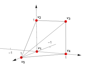
We first consider the case when . We take the twisting parameters to be given by , with as in the explicit solutions. We also take the R-symmetry vector to be , which we notice is proportional to , and assume that it is the critical vector, as just mentioned. The toric data can be obtained from that of in (3.3) with (for one has ) and is given by the following six inward pointing normal vectors
| (4.60) |
The toric diagram is shown in Figure 4 in section 4.6. Of the six Kähler class parameters, , only three are independent and, after some analysis, one can show that these can be taken to be , and . With the given R-symmetry vector, we find that the constraint equation (4.9) and the flux quantization conditions in (4.10), (4.11) are all satisfied providing that
| (4.61) |
where and . Indeed we find that the fluxes are given by
| (4.62) |
To ensure that these are integers we demand that . Furthermore, the R-charges are given by
| (4.63) |
with . It is interesting to point out that while the geometry is quasi-regular for all values of (since ) the R-charges can be irrational. Notice also that when the R-charges are proportional to the fluxes, as in the universal twist solutions in section 4.3. Finally, after calculating the on-shell supersymmetric action (4.8), (4.17) we obtain
| (4.64) |
These expressions precisely agree with their counterparts in appendix C obtained by analysing the explicit supergravity solutions.
As an aside we note that given the Kähler class parameters in (4.4) and our choice of , the master volume as a function of takes the simple form
| (4.65) |
As we recalled in section 4.3, a dual quiver gauge theory for was proposed in [47] and a calculation of the large topologically twisted index on was presented in [29]. Indeed for (which corresponds to the universal twist) we have already noted that the geometric results are in agreement with the field theory results888Which requires setting in [29].. It would be interesting to find a dual field theory interpretation of the -deformed geometry that we discussed above.
We now consider the case when , which is very similar. We take the twisting parameters to be given by , with as in the explicit solutions. We also take the R-symmetry vector to be , which is again proportional to , and we again assume that it is the critical vector. The toric data for can be obtained from in (3.2) with and :
| (4.66) |
Of the five Kähler class parameters, , only two are independent and, after some analysis, one can show that these can be taken to be and . With the given R-symmetry vector, we find that the constraint equation (4.9) and the flux quantization conditions (4.10), (4.11) are all satisfied providing that
| (4.67) |
where and . The fluxes are given by
| (4.68) |
We again demand in order that these are all integers. The R-charges are
| (4.69) |
with , and these can be irrational. One can again check that the R-charges are proportional to the fluxes when , which is the case of the universal twist solution. Finally, for the on-shell supersymmetric action (4.8), (4.17) we obtain
| (4.70) |
These expressions precisely agree with their counterparts in appendix C obtained by analysing the explicit supergravity solutions.
4.5 Conifold example
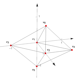
In the reminder of this section we will study examples of the form , with toric , with known dual three-dimensional field theories. Specifically, we start here considering as the link of the complex cone obtained by taking the product of the complex plane with the conifold singularity. This complex cone is specified by five inward pointing normal vectors given by
| (4.71) |
The toric diagram is obtained by projecting on the vertices in (4.5) and is shown in Figure 3.
The presence of the square face in the toric diagram (as opposed to a triangle), indicates that the link of Conifold has worse-than-orbifold singularities. Specifically, the divisor associated with is a copy of the conifold, sitting at the origin of the complex plane , and this gives rise to an associated singularity on . As we explain in more detail in appendix A.3 some care is required in using the master volume formula. The diagnostic that the master volume formula is not, in general, calculating a volume is that the relation (2.36) is not satisfied unless we impose that the Kähler class parameters satisfy .
A procedure one can follow is to resolve the singularity by adding an extra line either from to or from to as illustrated in Figure 6 in appendix A.3. In both of these resolutions (2.36) is satisfied and from the one can construct two gauge invariant variables given by
| (4.72) |
Furthermore, when one sets in the associated master volume formulae one finds that the two expressions are equal and moreover they are equal to the master volume for the toric diagram in Figure 3, associated with the singular , after setting . Thus, we conclude that one can use the master volume formulae for associated with Figure 3 provided that one sets , and then checks a posteriori that one has a set-up consistent with flux quantization. An additional subtlety is that for the singular geometry we should not impose that all fluxes are integer, but instead only certain linear combinations, associated with the fact that it is these linear combinations that correspond to bona fide cycles of . We expect that this procedure should yield the same results as starting with the non-singular resolved geometries, associated with Figure 6, and then imposing an additional condition on the quantised fluxes, but we have not checked this in detail999It is difficult to explicitly carry out the extremization procedure at the algebraic level..
Proceeding with and with the master volume for Figure 3, we first solve the constraint equation (4.9) for , finding a long expression that we don’t record101010One finds that after substituting for , still has some dependence on , and . This is expected, because is not invariant under gauge transformations but it transforms as in (4.1).. We then solve the flux quantization condition (4.10) for finding
| (4.73) |
where we have now set . The sign ambiguity in solving for will get resolved after extremization and demanding that the entropy is positive. This issue arises in generic examples and we will not explicitly keep track of it. One can then use (4.73) to obtain expressions for the fluxes from (4.11) obtaining
| (4.74) |
and one can check that (4.13) is satisfied. Apart from these are not, in general integers. However, various linear combinations are, for example:
| (4.75) |
We can also work out the R-charges from (4.20) and we find
| (4.76) |
which satisfy (4.23). Various linear combinations of these expressions simplify, echoing the expressions in (4.5). Finally, we can then obtain an explicit form for the off-shell entropy function , using (4.8) (4.17) (or equivalently (4.15)) which is expressed in terms of , and . Up to an overall sign ambiguity (arising from (4.73)) we obtain
| (4.77) |
We can now compare these results with the field theory analysis, for genus , carried out in [29]. We first recall various aspects of the three-dimensional quiver gauge theory discussed in section 6.1 of [47]. This is an instance of a general family of “flavoured” quiver gauge theories with gauge group and three adjoint chiral fields . There are also three sets of fields , transforming in the fundamental and anti-fundamental representation of and associated with global symmetries. The superpotential reads
| (4.78) |
and the quiver diagram can be found in (5.48) of [29], whose notation we will follow below. As discussed in [47] the Conifold geometry corresponds to the theory with and (see Figure 3(b) of [47]). An important aspect of these models is that there is a quantum correction to the moduli space of vacua, due to the presence of monopole operators and , which satisfy the relation
| (4.79) |
When , this gives the Conifold geometry.
For generic values of these three-dimensional theories flow to a SCFT in the IR, with gravity dual AdS, where is the Sasaki-Einstein base of the Calabi-Yau cone singularity. In [44] it was shown that the large limit of the free energy, , obtained from the exact localized partition function on , takes the form (4.48), where is the Sasakian volume.
To compare the field theory with the geometry, we need to relate the fields of the quiver with the toric data of the singularity. In particular, the fields correspond to linear combinations of the toric divisors and the field-divisors map (4.59) may be obtained by employing the perfect matching variables [47]. This map was explicitly given in [44] for the above class of theories and for the case of the Conifold model reads, in the notation of [44],
| (4.80) |
where the perfect matching variables are associated to the toric data (4.5) as in Table 1 below.
With this map, we can parametrize the R-charges of the fields in the quiver in terms of the geometric R-charges , defined using the volumes of supersymmetric five-dimensional toric submanifolds , through the relation (4.53).
We now consider compactifying this quiver gauge theory on a Riemann surface , with a twist that is parametrized by integer valued flavour magnetic fluxes for the fields with units of flux, as required for supersymmetry. Assuming that the theory flows to a SCQM in the IR, we expect that the dual supergravity solution will be an AdS solution of supergravity with a fibration of a toric over and we can compare with our geometric results above. To proceed, we can use the map (4.80) to relate the R-charges of the fields, , with the geometric R-charges, (see (4.21)), via
| (4.81) |
and
| (4.82) |
where in the last equalities we used the parametrization (4.5) coming from the geometry. We also define (see (2.3) of [44])
| (4.83) |
Notice that the R-charges of the adjoint fields satisfy , as implied by supersymmetry.
Similarly, the fluxes of the fields can be identified with a set of geometric flux parameters (see (4.12)) in an entirely analogous manner, namely
| (4.84) |
and
| (4.85) |
where in the last equalities we used the parametrization (4.5) coming from the geometry. Notice that the fluxes of the adjoint fields satisfy , as implied by supersymmetry.
Finally, for the case of , we can compare with the large limit for the off-shell index on , , that was computed in [29]. Specifically, equation (5.56) of this reference111111To compare with the expression in [29] one should relate the variables used here to that used in [29] as . gives
| (4.86) |
with
| (4.87) |
Using the dictionary given in (4.5)–(4.5), we see that the off-shell entropy function (4.5) calculated from the geometry side cannot agree with the expression given in (4.86), since the former depends on whereas the latter does not (only the monopole fluxes depend on ). However, remarkably, if we impose121212The relation (4.88) is equivalent to the particular relation among monopole charges in the field theory variables. Interestingly, we also find agreement of (4.5) and (4.86) if we restrict to the subspace of , without imposing any relation among the fluxes . the additional constraint on the geometric fluxes that
| (4.88) |
then we find our off-shell entropy geometric result , obtained from (4.5), agrees with the expression in (4.86). The result reported in [29] corresponds to setting .
We can make a further connection between geometry and field theory by relating our master volume with the function that is proportional to the large limit of the matrix model Bethe potential and determines the index. This was shown [29] to coincide with the large limit of the free energy on of the field theory, namely
| (4.89) |
Recall from (4.51) that in the universal twist case we found that the off-shell master volume is related to the large free energy as . We can show that this relation also holds in the Conifold setting. To see this, from [29] we have that
| (4.90) |
and using the dictionary above we find
| (4.91) |
On the other hand, evaluating the master volume with and obtained from (4.73), we find
| (4.92) |
where both sides are regarded as functions of ).
We conclude this subsection by considering the expression (4.34) for the supersymmetric action in the context of the present example. Recall that when the change of variables (4.29) between the and the is invertible, we can write the master volume as a function of the and the off-shell supersymmetric action takes the form (4.34). For the Conifold example, we imposed on the Kähler classes, leaving us with four variables (before imposing the constraint or flux quantisation conditions), implying that we cannot carry out such an invertible change of variables. Nevertheless, we can re-write the off-shell master volume in terms of the variables, where an ambiguity is fixed by requiring that this is a homogeneous function of degree two. Namely we have
| (4.93) |
We can now take derivatives of in (4.93) with respect to and after substituting for and from (4.5) and (4.5), we find that (4.34) gives .
4.6 example
In this section, we will revisit the case of , that we already studied in section 4.4 in the context of explicit supergravity solutions. In particular here we will be able to make a connection with a field theory result for the twisted topological index that was given in [29]. Recall that the toric data is specified by the vectors
| (4.94) |
The corresponding toric diagram, obtained by projecting the vertices in (4.6) onto , is given in Figure 4.
To connect with the field theory analysis of [29] we will consider the fibration to be of the form
| (4.95) |
where is an arbitrary integer and . Due to the algebraic complexity of the extremal problem, to proceed we will make a simplifying assumption on the Reeb vector, consistent with the symmetries associated with (4.95), which then needs to be justified a posteriori. Specifically, we assume
| (4.96) |
This implies, via (4.23), that we are assuming that the R-charges satisfy , and in addition to . There are similar conditions for the fluxes due to (4.13) and (4.95).
Within this ansatz we can construct three linear combinations of the Kähler parameters, invariant under the gauge transformations (2.37), given by
| (4.97) |
In terms of these variables, the master volume reads
| (4.98) |
Note if we set , and also131313Including the parameter in the analysis, should be associated with the more general explicit supergravity solutions discussed in section 6.3 of [28]. then we are within the framework of the explicit supergravity solutions that we discussed in section 4.4. We continue with .
Next we can solve the constraint equation (4.9) for . We also find that the expression for in (4.10) is linear in and hence can be simply solved for . At this point we would next like to solve two of the equations for the fluxes given in (4.11) for and . However, it is difficult to solve the simultaneous polynomial equations in closed form. However, we can get results matching with the field theory results using some inspired guesswork. Specifically, we make the further assumption that . With the given solution for we then have
| (4.99) |
Substituting this into the master volume we find
| (4.100) |
The R-charges take the form
| (4.101) |
while the fluxes are given by
| (4.102) |
Finally, we find the following off-shell expression for the entropy
| (4.103) |
Remarkably, for this agrees precisely computation of the large limit of the index presented in (5.47) of [29], after identifying and , as we discuss further below. Furthermore, there is also agreement between the large free energy and the expression for the master volume given in (4.99).
An important point is that we have a consistent framework provided that the are all integer. This is possible provided that the extremal point of the entropy function is such that the expression for the in (4.6) are all rational multiples of . We leave further investigation of this point for the future. It is worth noting, though, that if we set then this condition is satisfied. In addition, when both the master volume and the entropy do not depend on and the expressions agree with the corresponding expressions for the universal twist. However, noting that the R-charges are not proportional to the fluxes, we see that these solutions are not associated with the universal twist, but instead can be interpreted as a marginal deformation, parametrised by .
As in the previous subsection, we can compare these geometric results with the field theory analysis that was presented in [29], for genus . The relevant three-dimensional quiver gauge theory was discussed in section 6.2 of [47]; it is an instance of a family of “flavoured ABJM” theories, with gauge group and four bi-fundamental chiral fields . The flavour fields consist of four sets of fields , transforming in the fundamental or anti-fundamental representations of one of the two nodes. The associated quiver diagrams are drawn in Figure 6(a) of [47], and the superpotential is given by
| (4.104) |
In particular, the theory141414Interestingly, the case and corresponds to the conifold geometry that we discussed in the previous section. with and (see Figure 9 of [47]) corresponds to the geometry of relevance here. In this family of theories the monopole operators and satisfy the quantum relation
| (4.105) |
The large free energy on for the case was first computed in [43] and later extended to the full class of theories with arbitrary number of flavours in [44]. In this reference it was also shown that the free energy agrees with the expression (4.48) in terms of the Sasakian volume in the dual AdS supegravity solution. The large topologically twisted index on of these theories was calculated in [29].
Let us now focus on the model. The field-divisors map (4.59) that is needed to read off the charges of fields in the quiver is obtained using the perfect matching variables which were given in [47]. In the notation of that reference we have
| (4.106) |
where the perfect matching variables are associated to the toric data151515The toric data given in (4.6) and that associated with Figure 9 of [47] are related via an transformation given by (4.110) acting on the in (4.6), followed by a reflection of the third coordinate . (4.6) as in Table 2 below.
We now consider compactifying this quiver gauge theory on a Riemann surface , with a twist that is parametrized by integer valued flavour magnetic fluxes for the fields with , as required for supersymmetry.
Assuming that the theory flows to a SCQM in the IR, we expect that the dual supergravity solution will be an AdS solution of supergravity with a fibration of a toric over and we can compare with our geometric results above. Using the relations (4.106) we can express the R-charges of the fields, , in terms of the geometric R-charges, , via
| (4.111) |
and
| (4.112) |
Here the equalities , follow from our initial restriction of . Notice that the monopole charge is simply given by
| (4.113) |
and of course the R-charges satisfy . Analogously, the fluxes associated to the fields can be identified with a set of geometric flux parameters (see (4.12)) via
| (4.114) |
and
| (4.115) |
Notice that the fluxes of the adjoint fields satisfy , as implied by supersymmetry, while , mirroring (4.113) and . Again, the equalities , follow from our initial restriction of . As already noted above the fluxes given in (4.114) are not rational a priori and their values depend on the , which a dynamical variable. These should be held fixed while extremizing the index, given below, as a function of . This is to be contrasted with the example discussed in the previous subsection, where the fluxes (4.5) were manifestly integer and independent of the . It would be interesting to determine the precise conditions when a corresponding supergravity solution exists.
For the case of , we can compare our results with the large limit for the off-shell index on , , that was computed in [29]. Specifically, equation (5.46) of this reference161616To compare with the expression in [29] one should relate the variables used here to that used in [29] as . gives
| (4.116) |
which remarkably agrees with (4.103), after identifying and using (4.113).
As for the Conifold example, we find that the master volume in (4.100) is related to the large free energy and Bethe potential as
| (4.117) |
which we can also write as a homogeneous function of the geometric R charges, namely
| (4.118) |
with . Using this, we find that indeed
| (4.119) |
holds true.
We conclude by making contact with the results for the universal twist discussed in section 4.3. Setting we find the following
| (4.120) |
with , and the values of the entropy function and master volume reduce to
| (4.121) |
which are the values obtained in section 4.3. Although the parameter does not enter these expressions, nor the following field theory fluxes,
| (4.122) |
we have and . When we precisely recover the universal twist. However, when , as noted earlier we don’t have and, corresponds to a marginal deformation of the universal twist.
4.7 SPP example
In this section we consider another example of the form , with toric . Specifically, is the link of a toric Calabi-Yau 4-fold singularity that is closely related to the 3-fold singularity known as the suspended pinch point (SPP). In a slight abuse of terminology, we will refer to it as the SPP 4-fold singularity. The dual field theory is a known quiver Chern-Simons theory which we will recall momentarily, and its Abelian (i.e. rank ) mesonic vacuum moduli space is precisely the SPP 4-fold singularity. In the genus zero case, , the large limit of the twisted topological index on index was computed in [1]. In this subsection we will use our new formalism to recover the results of [1] from the gravitational point of view.
The SPP 4-fold singularity is labeled by an integer , which parametrizes the Chern-Simons levels in the dual gauge theory, and for simplicity we will set in the following. The toric diagram171717The model is a special case of a family of quiver theories labeled by two integers , known as , for which the corresponding toric diagram has eight vertices, given in (A.4). The case of SPP is for which the eight vertices degenerate to six; see for example [48]. has six vertices associated with six inward pointing normal vectors which we write as
| (4.123) |
The toric diagram is obtained by projecting on the vertices in (4.7) and is shown in Figure 5. Notice that this has a manifest symmetry along the axis of the Figure (the third entry in (4.7)). The presence of the square face in the diagram reveals that, like in the preceding subsection, this is a case with worse-than-orbifold singularities.
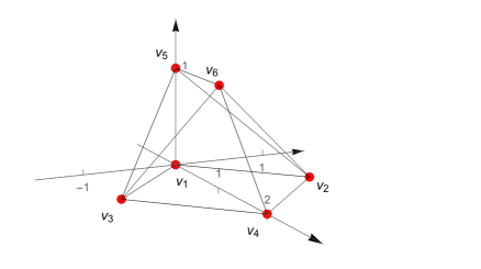
As in the section 4.5 we can use our master volume formulae for the toric diagram in Figure 5, but we must suitably restrict the Kähler class parameters. By resolving the toric diagram by adding in an extra line either from to or from to we can obtain master volume formulae that satisfy (2.36) and hence we can introduce gauge invariant variables and that are explicitly given in (A.4). We can proceed with the toric diagram in Figure 5 provided that we set . In fact the algebraic expressions are still rather unwieldy so we will make some additional assumptions in order to connect with the results of [32]. We will assume that the genus and consider a one-parameter family of fibrations, parametrised by , given by
| (4.124) |
with , as usual. Associated with these fibrations, which preserves certain symmetries, we take the trial R-symmetry vector to be
| (4.125) |
It is worth noting that we are not in the universal twist class181818To see this, note that a necessary requirement for the universal twist is that , as in (4.35), but this is satisfied if and only if . However, is not a critical point of the Sasaki volume (A.14), whose extremum is found at an irrational value of [42], in agreement with the fact that the SPP is not associated with a quasi-regular Sasaki-metric.. With this choice of fibration parameters, we find that is consistent, a posteriori, to not only set , which we must do to use the master volume formula, but also to impose and which then implies that , and .
We can now implement our general procedure to compute the off-shell entropy function . We first solve the constraint equation (4.37) for . We next solve (4.39) for finding
| (4.126) |
The fluxes in (4.38) are then given by
| (4.127) |
While and are integers, are not, in general. However, we do have
| (4.128) |
We will see that these fluxes precisely agree with those in the field theory; we expect that from a geometric point of view these can also be directly justified by determining the bona fide cycles in and then demanding that the associated fluxes are all integers. Furthermore, the geometric R-charges can be computed using formula (4.20) to get
| (4.129) |
and one can check that . Finally, the off-shell entropy function is computed to be
| (4.130) |
As in previous examples there is an overall sign ambiguity, not explicitly displayed, associated with solving for in (4.126), and can be fixed by demanding that the on-shell value, obtained by extremizing with respect to , is positive.
We can now compare these results with the field theory analysis, for , carried out in [1]. We first recall various aspects of the three-dimensional quiver gauge theory. The gauge group is and there are three doublets of bi-fundamental chiral fields . The fields and transform in the fundamental and anti-fundamental of a residual global symmetry, while the bi-fundamental and the adjoint field are singlets under this symmetry. The quiver diagram can be found in Figure 1 of [1] and the superpotential reads
| (4.131) |
The R-charges of the fields, , all depend on one parameter, which we denote by (and will shortly be identified as in the geometry), via
| (4.132) |
To see this we use the fact that each monomial in must have R-charge equal to 2, and also that the symmetry implies that fields in a doublet have equal R-charges. This implies the conditions on , given in (4.132) as well as . To deduce that one can invoke a symmetry of the quiver and superpotential that acts on the fields as , , .
This three-dimensional theory flows to a SCFT in the IR, with gravity dual AdS, where is the Sasaki-Einstein base of the SPP Calabi-Yau cone singularity. In [42] it was shown that the large limit of the free energy, , obtained from the exact localized partition function on , takes the form (4.48), with the Sasakian volume given in (A.14). Moreover the R-charges of the fields in the quiver may be expressed in terms of the geometric R-charges , defined using the volumes of supersymmetric five-dimensional toric submanifolds , through the relation (4.53).
The fields in the quiver field theory correspond to linear combinations of these toric divisors and, furthermore, the field-divisors map (4.59) may be obtained by employing the perfect matching variables. For the SPP singularity this map was given in [32], and in the notation of that reference reads
| (4.133) |
where the perfect matching variables are associated to the toric data191919The toric diagram here and that used in [32] are related via an transformation given by (4.137) acting on the in (4.7). (4.7) as in Table 3 below.
We now consider compactifying this quiver gauge theory on a Riemann surface , with a twist that is parametrized by integer valued flavour magnetic fluxes for the fields , respecting the global symmetries of the theory. Assuming that the theory flows to a SCQM in the IR, we expect that the dual supergravity solution will be an AdS solution of supergravity with a fibration of a toric over and we can compare with our geometric results above. To compare with the known field theory results of [1] we restrict our considerations to the following fluxes
| (4.138) |
where . In particular, one can check that every term in the superpotential (4.78) has units of flux, as required for supersymmetry. Next, we can use the map (4.7) to relate the R-charges of the fields, , with the geometric R-charges, (see (4.21)), via
| (4.139) |
Then from (4.132) we have
| (4.140) |
exactly as in the geometric expressions (4.7). Indeed, comparing to the latter allows us to identify
| (4.141) |
Similarly, the fluxes of the fields can be identified with a set of geometric flux parameters (see (4.12)) in an entirely analogous manner e.g. etc. For the specific fluxes that we want to consider, given in (4.138), we conclude that the geometric flux parameters are
| (4.142) |
Notice in particular, that there is not a quantization condition on and individually, but just on their sum. This is again in exact agreement with the geometric expressions (4.7).
To further compare with the geometric results we need to identify the twist parameters , , that define the geometric fibration of over , and which appear in (4.8)-(4.11). To do this, we can use the relation (4.13):
| (4.143) |
Using the toric data (4.7), along with the relations (4.7) obtained from field theory we deduce that the relationship between the geometric twist and the field theory twist is given by , which is precisely what we assumed on the geometry side in (4.124).
Finally, for the case of , with the field theory data for the R-charges , determined by in (4.132), and the magnetic fluxes , determined by in (4.138), the large limit for the off-shell index on , , that was computed in Appendix B of [1]; see equation (B.19) of this reference202020To match the expression in (B.19) of [1] one should relate the variable used here to that used in [1], , via ., namely
| (4.144) |
Remarkably, this exactly agrees with the geometric result in (4.130), for the restrictions on given in (4.124), (4.125) after setting , identifying , and taking the upper sign.
From our analysis of the geometry we can obtain the following off-shell expression for the master volume
| (4.145) |
To obtain this we used (4.125), the conditions on the Kähler class parameters, , and , and we have fixed the sign ambiguity arising from solving (4.126). Using (A.14), (4.48) we can again relate this to the off-shell free energy of the dual SCFT on via
| (4.146) |
Furthermore, the following relation between the master volume and the trial entropy function holds
| (4.147) |
consistent with the field theory results in appendix B of [1].
4.8 Connection to the index theorem of [1]
In the above examples we have seen that our entropy function coincides, off-shell, with the large limit of the topologically twisted index, , after using the dictionary between the geometric and field theory quantities. In this section, we will place these results in a more general context, making a closer comparison with the index theorem presented in [1]. A key ingredient is the result for the entropy function given in (4.34) in terms of the variables , that we discussed in section 4.2.
The main results of [1] were in the context of , non-chiral, quiver gauge theories in , with matter fields transforming in the adjoint and bi-fundamental representations of the gauge group, as well as “flavour” fields that transform in the (anti-)fundamental representations. Below we will restrict to the class of flavoured theories, with quantum corrected moduli spaces, that were considered in [47], but we expect that a similar connection between and will hold more generally, for the class of theories considered in [1] (indeed, the SPP example is not a flavoured model). We will also further restrict to cases where the field-divisor map (4.59) is invertible, which includes the Conifold example of section 4.5 and the example of section 4.6.
For this class of field theories the geometric R-charges, , and fluxes, , are related to the field theory R-charges, , and magnetic fluxes, , by invertible linear relationships of the form
| (4.148) |
where the index here runs over the adjoint and bi-fundamental chiral fields in the quiver, as well as the diagonal monopole operators and , but not the (anti-) fundamentals. Using (4.148) in (4.34) one quickly deduces that
| (4.149) |
Furthermore, if212121Note that this does not seem to be the case for the example of that we discussed in section 4.4. With the assumptions made in that section we have , and the free energy on is given by and is only related to via (4.150) when , which is the case of the universal twist. the master volume coincides with the free energy via222222As we have noted several times, sign ambiguities arise in carrying out the extremal problem which we are not explicitly writing.
| (4.150) |
we can conclude that
| (4.151) |
which has exactly the form of the index theorem discussed in [1].
In the field theory result of [1] the sum over the index “” runs a priori over all the chiral fields in the quiver, namely the adjoint, the bi-fiundamentals, as well as the (anti-)fundamental flavours, and also includes contributions from the magnetic fluxes and fugacities associated with the topological symmetry of the theories. However, the large free energy depends on the topological symmetry charges only through the combination and the contribution of the (anti-)fundamental fields can always be rewritten in terms of adjoint and bi-fundamental fields, using the constraints imposed by the superpotential [44].
Returning to our formula (4.151), it is illuminating to extract from the sum the contributions of the monopole operators and . After defining the linear combinations
| (4.152) |
we can rewrite (4.151) as
| (4.153) |
where the prime in the sum indicates that it now does not include the monopole operators (nor, as usual, the (anti-)fundamental fields) and the second line follows from the fact that in the large limit is independent [44] of as mentioned above. This result can be favourably compared with the field theory results of [1] after recalling that here we are using a set of constrained variables, such that the master volume/free energy is a homogeneous function.
Let us now return to the conifold example of section 4.5 and use this general expression to discuss further the restriction on the fluxes (4.88). The geometric fluxes are related to the variables introduced above as
| (4.154) |
and to get agreement with [29] we had to impose . Indeed we find that the first two terms in (4.86) match the primed sum in (4.8), while the remainder term exactly agrees if . We then conclude that in the field theory calculation in [29] it has been assumed that , but it should be possible to incorporate a generic value of that would then fully agree with our geometric result.
5 Discussion
In this paper we have extended the results of [5, 16] concerning a geometric extremal problem, analogous to volume minimization in Sasakian geometry [10, 11], that allows one to calculate key properties of supersymmetric AdS and AdS solutions. Specifically, we have provided a formalism based on a master volume that allows one to study AdS solutions with toric as well as AdS solutions where is a fibration of a toric over a Riemann surface . In both cases can be non-convex toric [5].
The results concerning the latter class of solutions comprise a geometric dual of -extremization [6] for the class of , SCFTs obtained from compactifying toric , SCFTs (i.e. dual to AdS solutions with toric ) on a Riemann surface , with a partial topological twist. We expect that this class of AdS solutions will generically arise as the near horizon limit of supersymmetric black hole solutions that asymptotically approach AdS in the UV. The supersymmetric action to be extremized in our procedure can also be interpreted, after suitable normalization, as an entropy function, which reduces to the Bekenstein-Hawking entropy of the black hole at the critical point. Thus, our results can be used to calculate the entropy of large classes of supersymmetric black holes, independently of a detailed knowledge of the full supergravity solutions, just assuming that they exist, thus extending [6] to a much more general class of black hole solutions. Furthermore, when it is possible to carry out a calculation of the associated topological index in the field theory using localization techniques, and assuming that they agree, one will then have a microscopic state counting interpretation of the black hole entropy for this class of black holes.
We illustrated the extremization procedure in various examples. We highlighted that the formalism can be used, with care, for toric singularities with worse-than-orbifold singularities. This is important since many examples in the literature are associated with such singular . Most strikingly, in the examples that we studied we are able to match the off-shell entropy function and the off-shell field theory results for the large limits of the partition functions on (i.e. the topological twisted index). In addition we were also able to obtain some general results in section 4.8. It would certainly be very interesting determine the necessary and sufficient conditions for the relations discussed there to hold, in order to aim for a general proof of the equivalence of -extremization and -extremization, analogous to the result of [17] who analysed a similar problem for the class of AdS solutions with a fibration of a toric over .
In a slightly different direction, it would certainly be interesting to construct a master volume formula for AdS solutions with toric . This would provide a direct geometric dual of the version of -extremization for toric and may well help in establishing a precise field theory version of -extremization in . It would also be very interesting to determine whether or not this more general class of AdS solutions can arise as the near horizon limit of black holes.
Acknowledgments
We thank Noppadol Mekareeya and Alberto Zaffaroni for discussions. JPG is supported by the European Research Council under the European Union’s Seventh Framework Programme (FP7/2007-2013), ERC Grant agreement ADG 339140. JPG is also supported by STFC grant ST/P000762/1, EPSRC grant EP/K034456/1, as a KIAS Scholar and as a Visiting Fellow at the Perimeter Institute. DM is supported in part by the STFC grant ST/P000258/1.
Appendix A Computation of the master volume in examples
In this appendix we give some details of the computation of the master volume formula in the examples that we studied in the paper. We recall the master volume formula is given by
| (A.1) |
where
| (A.2) |
Here is the number of vertices , , of the toric diagram and for each vertex, denotes the number of edges meeting there.
A.1
The toric diagram for is given in Figure 1, where we labeled the vertices as in [31]. In particular, we have
| (A.3) |
The polytope has vertices, with and . The vectors needed to evaluate (A.1) are given in Table 4. The ordering of the vectors can be obtained by going counter-clockwise around a vertex when viewed from outside the toric diagram in Figure 2. One can explicitly check that this ensures that each term in the sums in (A.1) is positive for inside the Reeb cone.
The resulting formula fits in a few lines and we do not report it here.
A.2
The toric diagram for is given in Figure 2, where recall the vertices are given by
| (A.4) |
The polytope has vertices, with . The vectors needed to evaluate (A.1) are given in Table 5. Again the ordering of the vectors can be obtained by going counter-clockwise around a vertex when viewed from outside the toric diagram in Figure 3 of [31].
The formula of the master volume is lengthy, so we do not write it down.
A.3 = Link of Conifold
The toric diagram for the toric Kähler cone Conifold is given in Figure 3 and the vertices are given by
| (A.5) |
An important feature of this example is that the square face in the toric diagram shows that the link has worse-than-orbifold singularities. Indeed, the toric divisor associated with is a copy of the conifold. The polytope has vertices, with and . The vectors needed to evaluate the master volume (A.1) are given in Table 6. As usual, the ordering of the vectors can be obtained by going counter-clockwise around a vertex when viewed from outside the toric diagram in Figure 3.
It is important to note that the relation (2.36) is not satisfied for this example in general. However, it is satisfied when we impose . This is precisely a consequence of the fact that has worse-than-orbifold singularities. Specifically, when the master volume formula is no longer calculating a volume.
Further insight can be obtained by resolving the conifold singularity on . This can be done in two different ways, associated with a flop transition of the conifold. In each case we keep the same vertices but add in an extra line, either stretching from to or from to as in Figure 6.
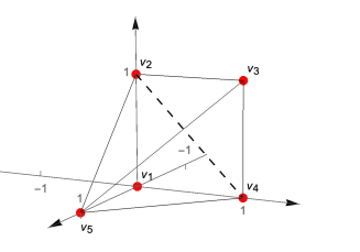
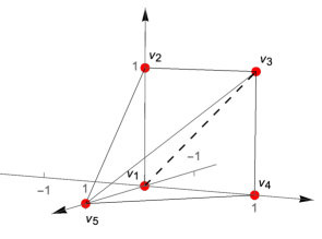
Notice that all faces of the toric diagram are triangles and so there are now at worst, only orbifold singularities. To calculate the master volume for these two cases we note that in the first we have and while in the second we have and . The vectors needed to evaluate (A.1) are given in the left and right hand tables in Table 7, respectively.
For each of these two cases, we find that the expression for now satisfies (2.36). By analysing (2.37) we can obtain two gauge-invariant combinations of the given by
| (A.6) |
In terms of these variables, the volumes take the form
| (A.7) |
for the two different resolved geometries, respectively, and . Furthermore, one can check that for the special Kähler class with , then we get
| (A.8) |
and, importantly, this agrees with the expression for for the link of Conifold, with its worse-than-orbifold singularities, when .
The Sasaki Kähler class is obtained when , or equivalently when and . Extremizing this volume while holding fixed, at the critical point we recover the Sasakian volume formula232323One can check that this volume is twice that given in equation (3.33) of [31] for the case of with , consistent with the fact that this is a orbifold of the link of Conifold.
| (A.9) |
with the critical Reeb vector given by
| (A.10) |
A.4 = Link of SPP
The toric diagram for the SPP 4-fold singularity comprises of the following six vertices
| (A.11) |
The toric diagram, obtained by projecting the vertices in (A.4) onto , is shown in Figure 5. Notice that this has a manifest reflection symmetry along the axis (third entry). Just like the case of Conifold that we considered in the previous subsection the link of this singularity has worse-than-orbifold singularities as revealed by the presence of a non-triangular face bounded by , , and .
In general the relation (2.36) is not satisfied for this example, but it is satisfied when we impose . As in the case of Conifold this is again due to the presence of worse-than-orbifold singularities and we can proceed in a similar manner. One can consider two resolutions obtained by adding in an extra line in the toric diagram, either from to or from to . In each case one gets a master volume formula, and , respectively, both of which satisfy the relation (2.36). For these cases we can then construct three gauge invariant variables given by
| (A.12) |
We find that and moreover when then is precisely the same as the master volume calculated from the toric diagram in Figure 5 after setting .
An expression that we found useful is when and in which case ,
| (A.13) |
The case of the Sasakian volume is obtained by further setting , and hence . Further extremizing while holding we recover the Sasakian volume formula given in equation (5.5) of [42], namely
| (A.14) |
with the Reeb vector parameterised as
| (A.15) |
and at the critical point.
Appendix B Homology relations and twisting
In this appendix we give a proof of the homology relation (B.8) that leads to (4.13), extending some of the arguments used in [49].
For simplicity we assume that is simply connected, which since we may always do by passing to a finite covering space. Recall that the cone may be realized as a Kähler quotient . The torus arises as follows. Define the linear map
| (B.1) |
Here denotes the standard orthonormal basis of , with components . Since also maps to , (B.1) induces a corresponding map of tori , and the torus is precisely the kernel of this map. It is generated by an integer matrix , , satisfying
| (B.2) |
which specifies the embedding . The toric action on is then via the quotient . More physically, the above construction may be viewed as a gauged linear sigma model with complex fields and charges specified by , with being the vacuum moduli space of this theory.
In order to fibre (or equivalently ) over a Riemann surface , we may first fibre over . To do so we must first lift the action on to , which means specifying , , satisfying
| (B.3) |
where denotes the standard orthonormal basis of . In components (B.3) reads
| (B.4) |
Of course, the choice of each is unique only up to the kernel of , generated by . Geometrically, this is because is precisely a Kähler quotient of via the torus generated by this kernel. By construction, the charge of the th coordinate of under the th is . We then construct the associated bundle
| (B.5) |
The space is the total space of a fibration over , where we twist the th action on via the line bundle , . This means that may be regarded as a coordinate on the fibre of , where . The fibred geometry we are interested in is
| (B.6) |
where we take a Kähler quotient of the fibres in (B.5), and set to obtain .
Next we may define the torus-invariant seven-manifolds via in the above construction. In we may view the as sections of complex line bundles over . These are sections of line bundles, rather than functions, because is charged both under the torus that we quotient by, and is also fibred over as . Consider now the 4 line bundles
| (B.7) |
The restriction of to each fibre is a trivial line bundle over that fibre. This follows from (B.2), where recall that generates the torus action on . This implies that are invariant under , and so the sections of are simply complex-valued functions on each fibre . On the other hand, (B.4) says that these sections of have charge under the th toric . As such, we may identify , where is the projection to the base. Taking the first Chern class of (B.7) and applying Poincaré duality then precisely gives
| (B.8) |
where is the Poincaré dual to . Integrating the seven-form flux of these cycles and using (B.8) then immediately leads to (4.13).
Finally, let us comment on (4.143), which recall arises in the field theory analysis. Here by definition is precisely the twisting of the th gauged linear sigma model field over the Riemann surface . On the other hand, in our geometric construction above the th gauged linear sigma model field is precisely the coordinate on , and thus we may identify
| (B.9) |
Thus in the bundle defined by (B.5), the fibre coordinate is precisely a section of . On the other hand, (B.4) then implies
| (B.10) |
which is precisely (4.143).
Appendix C Explicit supergravity solutions
Here we further analyse a class of explicit supergravity solutions of the form AdS that were first discussed in section 6.3 of [28] and were recently discussed in section 4.3.1 of [8]. The eight-dimensional Kähler base space used for the construction of the solutions is given by a product of Kähler-Einstein metrics
| (C.1) |
where is taken to have positive curvature. The Ricci form is given by
| (C.2) |
where the ’s are the associated Kähler forms, are constants and, without loss of generality, we can take . In order to solve the equation on the eight-dimensional manifold we should take . One of the two-dimensional Kähler-Einstein spaces is always a Riemann surface of genus , which we take to be . The range of is then . There are three cases to consider. First when and then is also a Riemann surface with genus . Second when and , then is a Riemann surface with genus and finally when and , then is a Riemann surface with genus . For simplicity of presentation we only present details of the analysis for the latter case, which is the case relevant for the analysis in section 4.
We relabel and continue with . The eight-dimensional Kähler base space can then be written
| (C.3) |
where is the metric on the unit radius round two-sphere, so that , and is a Riemann surface of genus with . It will also be useful to note that since the metric on satisfies , we have where is a topological integer for . For further discussion of this result see, for example, appendix B of [27], where one can also find a discussion of the Fano index, , of . Here we will need the fact that if we consider a set of two-cycles that generate , then we have for . For we have and . For we have and . For the del Pezzos, , , we have and , as well as , and .
The metric on appearing in the AdS2 solution as in (4.1) is given by
| (C.4) |
where is a local one-form satisfying and . By defining to be a circle fibration over , we can then view in the solutions as being obtained by fibreing over . When we have special examples of the universal twist solutions, discussed in section 4.3; the cases and correspond to and , respectively. The two-form appearing in the four-form flux (4.1) is given by
| (C.5) |
For flux quantization we need the seven-form , which takes the form
| (C.6) |
where .
Regularity of the metric is ensured if parametrizes a circle with period , where . Thus, if is even then and if is odd then . Next we calculate the flux through the various seven-cycles. We first consider the seven-cycle obtained by fixing a point on , i.e. the circle fibred over , which is a copy of , and we obtain
| (C.7) |
with . We can also consider the cycle obtained by fixing a point on the as well as the cycle obtained as the fibration of over , where generate . After using (C.7), for these cycles we find, respectively,
| (C.8) |
with . We need to ensure that . By considering the ratio we conclude that we must have
| (C.9) |
which, interestingly, can be achieved for irrational (e.g. ). We can then suitably choose and hence so that . We also note that for the universal twist, when , we have and . We next calculate
| (C.10) |
When this expression can be recast in the form
| (C.11) |
using the fact that the volume of the regular Sasaki-Einstein metrics associated with circle fibrations over can be expressed as .
In the special case that is toric, i.e. , or , from (4.19), the R-charges associated with M5-branes wrapping toric divisors associated with five-cycles on (i.e. at a fixed point on ), are given by,
| (C.12) |
We now consider the case of , with and hence . In this case242424Note that if we took then we would have the regular orbifold . is . Two of the , which we take to be are associated with the circle fibration over , while sitting at the north and the south pole of the generic in (C.3), respectively. Similarly, we can consider sitting at the north and south pole of each of the two factors in leading to four more with . We then find
| (C.13) |
and one can check that . The labelling we have chosen is consistent with the toric data given by
| (C.14) |
as used in (3.3). One can directly obtain the R-symmetry vector and the integers defining the fibration, in the toric basis (C), by further analysing the associated Killing vectors in the explicit metric. However, it is more convenient to obtain them via the following method. For this example, we have verified that the identity (2.36), which we give again here:
| (C.15) |
holds. Therefore, we can immediately conclude that for any . In addition the fluxes are associated with the , in (C) with , while are associated with . Thus we have
| (C.16) |
Similarly, we can use the condition (4.13),
| (C.17) |
to conclude that . Notice that for all values of we have , as in the universal twist (4.35). For the special value of we also have , which is an additional condition that is required in order to obtain the universal twist solutions in section 4.3.
We now consider the case of , with and hence . In this case is . Two of the , which we take to be , are associated with the circle fibration over , while sitting at the north and the south pole of the generic in (C.3). Similarly, we can consider the product of the generic with the three two-spheres associated with the toric divisors of , leading to three more which we label . We then find
| (C.18) |
and again we have . The labelling we have chosen is consistent with the toric data given by
| (C.19) |
We find that the condition (4.23), which is valid for this example, implies for any . In addition the fluxes are associated with in (C) while , are associated with the , with . Thus we have
| (C.20) |
The condition (C.17) then implies . Notice that for all values of we again have , as in the universal twist (4.35). For the special value of we also have , for and , for ; the proportionality of the R-charges and the fluxes is an additional condition for the universal twist solutions in section 4.3.
In both of the above examples, the R-symmetry vector had rational entries and hence, as far as the geometry is concerned, the R-symmetry foliation is (quasi-)regular. Furthermore, when is rational all of the R-charges are also rational. However, when is irrational, and satisfying (C.9), the R-charges are irrational numbers.
References
- [1] S. M. Hosseini and A. Zaffaroni, “Large matrix models for 3d theories: twisted index, free energy and black holes,” JHEP 08 (2016) 064, arXiv:1604.03122 [hep-th].
- [2] K. A. Intriligator and B. Wecht, “The Exact superconformal R symmetry maximizes ,” Nucl. Phys. B667 (2003) 183–200, arXiv:hep-th/0304128 [hep-th].
- [3] F. Benini and N. Bobev, “Exact two-dimensional superconformal R-symmetry and c-extremization,” Phys. Rev. Lett. 110 no. 6, (2013) 061601, arXiv:1211.4030 [hep-th].
- [4] D. L. Jafferis, “The Exact Superconformal R-Symmetry Extremizes Z,” JHEP 05 (2012) 159, arXiv:1012.3210 [hep-th].
- [5] C. Couzens, J. P. Gauntlett, D. Martelli, and J. Sparks, “A geometric dual of -extremization,” JHEP 01 (2019) 212, arXiv:1810.11026 [hep-th].
- [6] F. Benini, K. Hristov, and A. Zaffaroni, “Black hole microstates in AdS4 from supersymmetric localization,” JHEP 05 (2016) 054, arXiv:1511.04085 [hep-th].
- [7] A. Cabo-Bizet, V. I. Giraldo-Rivera, and L. A. Pando Zayas, “Microstate counting of AdS4 hyperbolic black hole entropy via the topologically twisted index,” JHEP 08 (2017) 023, arXiv:1701.07893 [hep-th].
- [8] F. Azzurli, N. Bobev, P. M. Crichigno, V. S. Min, and A. Zaffaroni, “A universal counting of black hole microstates in AdS4,” JHEP 02 (2018) 054, arXiv:1707.04257 [hep-th].
- [9] F. Benini and A. Zaffaroni, “Supersymmetric partition functions on Riemann surfaces,” Proc. Symp. Pure Math. 96 (2017) 13–46, arXiv:1605.06120 [hep-th].
- [10] D. Martelli, J. Sparks, and S.-T. Yau, “The Geometric dual of -maximisation for Toric Sasaki-Einstein manifolds,” Commun. Math. Phys. 268 (2006) 39–65, arXiv:hep-th/0503183 [hep-th].
- [11] D. Martelli, J. Sparks, and S.-T. Yau, “Sasaki-Einstein manifolds and volume minimisation,” Commun. Math. Phys. 280 (2008) 611–673, arXiv:hep-th/0603021 [hep-th].
- [12] S. Giombi and I. R. Klebanov, “Interpolating between and ,” JHEP 03 (2015) 117, arXiv:1409.1937 [hep-th].
- [13] N. Kim, “AdS3 solutions of IIB supergravity from D3-branes,” JHEP 01 (2006) 094, arXiv:hep-th/0511029 [hep-th].
- [14] N. Kim and J.-D. Park, “Comments on AdS(2) solutions of D = 11 supergravity,” JHEP 09 (2006) 041, arXiv:hep-th/0607093.
- [15] J. P. Gauntlett and N. Kim, “Geometries with Killing Spinors and Supersymmetric AdS Solutions,” Commun. Math. Phys. 284 (2008) 897–918, arXiv:0710.2590 [hep-th].
- [16] J. P. Gauntlett, D. Martelli, and J. Sparks, “Toric geometry and the dual of -extremization,” JHEP 01 (2019) 204, arXiv:1812.05597 [hep-th].
- [17] S. M. Hosseini and A. Zaffaroni, “Proving the equivalence of -extremization and its gravitational dual for all toric quivers,” JHEP 03 (2019) 108, arXiv:1901.05977 [hep-th].
- [18] J. P. Gauntlett, O. A. P. Mac Conamhna, T. Mateos, and D. Waldram, “Supersymmetric AdS(3) solutions of type IIB supergravity,” Phys. Rev. Lett. 97 (2006) 171601, arXiv:hep-th/0606221 [hep-th].
- [19] S. M. Hosseini, K. Hristov, and A. Passias, “Holographic microstate counting for AdS4 black holes in massive IIA supergravity,” JHEP 10 (2017) 190, arXiv:1707.06884 [hep-th].
- [20] F. Benini, H. Khachatryan, and P. Milan, “Black hole entropy in massive Type IIA,” Class. Quant. Grav. 35 no. 3, (2018) 035004, arXiv:1707.06886 [hep-th].
- [21] N. Bobev, V. S. Min, and K. Pilch, “Mass-deformed ABJM and black holes in AdS4,” JHEP 03 (2018) 050, arXiv:1801.03135 [hep-th].
- [22] M. Suh, “Supersymmetric AdS6 black holes from F(4) gauged supergravity,” JHEP 01 (2019) 035, arXiv:1809.03517 [hep-th].
- [23] S. M. Hosseini, K. Hristov, A. Passias, and A. Zaffaroni, “6D attractors and black hole microstates,” JHEP 12 (2018) 001, arXiv:1809.10685 [hep-th].
- [24] M. Suh, “Supersymmetric black holes from matter coupled gauged supergravity,” JHEP 02 (2019) 108, arXiv:1810.00675 [hep-th].
- [25] J. P. Gauntlett, D. Martelli, J. Sparks, and S.-T. Yau, “Obstructions to the existence of Sasaki-Einstein metrics,” Commun. Math. Phys. 273 (2007) 803–827, arXiv:hep-th/0607080 [hep-th].
- [26] A. Futaki, H. Ono, and G. Wang, “Transverse Kahler geometry of Sasaki manifolds and toric Sasaki-Einstein manifolds,” J. Diff. Geom. 83 no. 3, (2009) 585–636, arXiv:math/0607586 [math-dg].
- [27] J. P. Gauntlett, O. A. Mac Conamhna, T. Mateos, and D. Waldram, “New supersymmetric AdS(3) solutions,” Phys.Rev. D74 (2006) 106007, arXiv:hep-th/0608055 [hep-th].
- [28] J. P. Gauntlett, N. Kim, and D. Waldram, “Supersymmetric AdS(3), AdS(2) and Bubble Solutions,” JHEP 04 (2007) 005, arXiv:hep-th/0612253 [hep-th].
- [29] S. M. Hosseini and N. Mekareeya, “Large topologically twisted index: necklace quivers, dualities, and Sasaki-Einstein spaces,” JHEP 08 (2016) 089, arXiv:1604.03397 [hep-th].
- [30] S. M. Hosseini and A. Zaffaroni, “Geometry of -extremization and black holes microstates,” arXiv:1904.04269 [hep-th].
- [31] D. Martelli and J. Sparks, “Notes on toric Sasaki-Einstein seven-manifolds and AdS(4) / CFT(3),” JHEP 11 (2008) 016, arXiv:0808.0904 [hep-th].
- [32] A. Hanany, D. Vegh, and A. Zaffaroni, “Brane Tilings and M2 Branes,” JHEP 03 (2009) 012, arXiv:0809.1440 [hep-th].
- [33] J. P. Gauntlett, S. Kim, and D. Waldram Unpublished notes, 2008 .
- [34] J. P. Gauntlett, D. Martelli, J. F. Sparks, and D. Waldram, “A New infinite class of Sasaki-Einstein manifolds,” Adv. Theor. Math. Phys. 8 no. 6, (2004) 987–1000, arXiv:hep-th/0403038 [hep-th].
- [35] D. Martelli and J. Sparks, “Toric geometry, Sasaki-Einstein manifolds and a new infinite class of AdS/CFT duals,” Commun. Math. Phys. 262 (2006) 51–89, arXiv:hep-th/0411238 [hep-th].
- [36] L. J. Romans, “Supersymmetric, cold and lukewarm black holes in cosmological Einstein-Maxwell theory,” Nucl. Phys. B383 (1992) 395–415, arXiv:hep-th/9203018 [hep-th].
- [37] M. M. Caldarelli and D. Klemm, “Supersymmetry of Anti-de Sitter black holes,” Nucl. Phys. B545 (1999) 434–460, arXiv:hep-th/9808097 [hep-th].
- [38] J. P. Gauntlett, N. Kim, S. Pakis, and D. Waldram, “Membranes wrapped on holomorphic curves,” Phys.Rev. D65 (2002) 026003, arXiv:hep-th/0105250 [hep-th].
- [39] J. P. Gauntlett and O. Varela, “Consistent Kaluza-Klein Reductions for General Supersymmetric AdS Solutions,” Phys. Rev. D76 (2007) 126007, arXiv:0707.2315 [hep-th].
- [40] C. Couzens, D. Martelli, and S. Schafer-Nameki, “F-theory and AdS3/CFT2 (2, 0),” JHEP 06 (2018) 008, arXiv:1712.07631 [hep-th].
- [41] C. P. Herzog, I. R. Klebanov, S. S. Pufu, and T. Tesileanu, “Multi-Matrix Models and Tri-Sasaki Einstein Spaces,” Phys. Rev. D83 (2011) 046001, arXiv:1011.5487 [hep-th].
- [42] D. Martelli and J. Sparks, “The large N limit of quiver matrix models and Sasaki-Einstein manifolds,” Phys. Rev. D84 (2011) 046008, arXiv:1102.5289 [hep-th].
- [43] S. Cheon, H. Kim, and N. Kim, “Calculating the partition function of N=2 Gauge theories on and AdS/CFT correspondence,” JHEP 05 (2011) 134, arXiv:1102.5565 [hep-th].
- [44] D. L. Jafferis, I. R. Klebanov, S. S. Pufu, and B. R. Safdi, “Towards the F-Theorem: N=2 Field Theories on the Three-Sphere,” JHEP 06 (2011) 102, arXiv:1103.1181 [hep-th].
- [45] F. Benini and A. Zaffaroni, “A topologically twisted index for three-dimensional supersymmetric theories,” JHEP 07 (2015) 127, arXiv:1504.03698 [hep-th].
- [46] D. Berenstein, C. P. Herzog, and I. R. Klebanov, “Baryon spectra and AdS /CFT correspondence,” JHEP 06 (2002) 047, arXiv:hep-th/0202150 [hep-th].
- [47] F. Benini, C. Closset, and S. Cremonesi, “Chiral flavors and M2-branes at toric CY4 singularities,” JHEP 02 (2010) 036, arXiv:0911.4127 [hep-th].
- [48] D. Farquet and J. Sparks, “Wilson loops and the geometry of matrix models in AdS4/CFT3,” JHEP 01 (2014) 083, arXiv:1304.0784 [hep-th].
- [49] S. Franco, A. Hanany, D. Martelli, J. Sparks, D. Vegh, and B. Wecht, “Gauge theories from toric geometry and brane tilings,” JHEP 01 (2006) 128, arXiv:hep-th/0505211 [hep-th].