Estimating the dark matter velocity anisotropy to the cluster edge

Abstract

Dark matter dominates the properties of large cosmological structures such as galaxy clusters, and the mass profiles of the dark matter have been measured for these equilibrated structures for years using X-rays, lensing or galaxy velocities. A new method has been proposed, which should allow us to estimate a dynamical property of the dark matter, namely the velocity anisotropy. For the gas a similar velocity anisotropy is zero due to frequent collisions, however, the collisionless nature of dark matter allows it to be non-trivial. Numerical simulations have for years found non-zero and radially varying dark matter velocity anisotropies. Here we employ the method proposed by Hansen & Pifaretti (2007), and developed by Høst et al. (2009) to estimate the dark matter velocity anisotropy in the bright galaxy cluster Perseus, to near 5 times the radii previously obtained. We find the dark matter velocity anisotropy to be consistent with the results of numerical simulations, however, still with large error-bars. At half the virial radius we find the velocity anisotropy to be non-zero at 1.7$\,\sigma$, lending support to the collisionless nature of dark matter.

1 Introduction

The global dynamics of the expanding universe is dominated by two invisible components, namely dark matter (DM) and dark energy (Planck Collaboration et al., 2018). In addition there exist independent gravitational observations of dark matter on smaller scales (Clowe et al., 2006). Despite the importance of dark matter in structure formation, we still have only limited knowledge about its fundamental properties.

From a basic point of view, DM is constituted of fundamental particles, characterized by their mass and interactions with other particles. These parameters can be tested through astronomical observations as well as in terrestrial experiments. Typically, cosmological observations measure a combination of these. For instance, if DM particles interact with photons, structure formation will be affected through the ratio of the interaction cross section and the DM particle mass, $\sigma_{\gamma-\mathrm{DM}}/M_{\mathrm{DM}}$ (Bœhm et al., 2002; Hinshaw et al., 2013). Similar constraints can be obtained for DM self-scattering or for various annihilation channels (for a list of references, see e.g. Zavala et al. (2013); Liu et al. (2016)). A range of accelerator and underground detector “null” observations have provided limits on the DM mass and interaction rates, e.g., from CMS, ATLAS, DarkSide-50, LUX (Lowette & for the CMS Collaboration, 2014; ATLAS Collaboration et al., 2015; Agnes et al., 2015; Faham, 2014). Basically these constraints indicate that the DM has only very limited interactions besides gravity.

Structure formation has been thoroughly investigated for many years using numerical simulations in a cosmological setting. The resulting structures include galaxies and clusters at various stages of equilibration. These simulations have revealed that the DM density profile, $\rho(r)$, of individual cosmological structures changes from having a fairly shallow profile in the central regions, $\gamma_{\rho}=d\,{\rm log}{\rho}/d{\rm log}r\approx-1$, to a much steeper fall off in the outer regions, $\gamma_{\rho}\approx-3$ (Navarro et al., 2010).

For the largest equilibrated structures like galaxy clusters there is fair agreement between the numerical predictions and observations concerning the central steepness (Pointecouteau, E. et al., 2005; Vikhlinin et al., 2006). However, for smaller structures like galaxies or dwarf galaxies, the observations have indicated that the central region has a shallower density profile than seen in numerical simulations (Salucci et al., 2007; Gilmore et al., 2007), and it is not entirely resolved whether this difference is because of significant self-interaction of the DM, or because of stellar, black hole, or supernova effects. The majority of recent state of the art simulations employing cold dark matter models with baryonic effects and stellar feedback tend to agree with observations (Amorisco et al., 2014; Santos-Santos et al., 2017; Dutton et al., 2018; Wheeler et al., 2018; Benitez-Llambay et al., 2018; Wetzel et al., 2016; Bullock et al., 2015; Teyssier et al., 2013), however some still do not find cores using this approach (Bose et al., 2018). Some efforts have been made with alternative dark matter models, but the results are thus far not fully conclusive (Di Cintio et al., 2017; Fitts et al., 2018; González-Samaniego et al., 2017).

Observationally it is very difficult to determine other properties of the DM structures besides the density profile. The density profile is a static quantity (not involving velocity), which arises from the zeroth moment of the Boltzmann equation (i.e. mass conservation). The first moment of the Boltzmann equation instead relates to momentum conservation, and here appears the first dynamical properties in the shape of the so-called dark matter velocity anisotropy.

The principal purpose of measuring the dark matter velocity anisotropy is to improve our knowledge of dark matter. The value of the velocity anisotropy depends on the magnitude of the dark matter self-interactions (Brinckmann et al., 2018), and hence a precise measurement of the velocity anisotropy in the inner halo region should allow us to constrain the dark matter collisionality. Furthermore, it has been suggested from theoretical considerations that there should be a correlation between the dark matter velocity anisotropy and the total mass profile (Hansen, 2009), and a future accurate measurement of both would allow testing this prediction. Finally, it is possible that the velocity anisotropy in the outer cluster regions could depend on cosmological parameters, even though, to our knowledge, this has not yet been thoroughly investigated. Hopefully an investigation like the one we are presenting here, will inspire simulators to make such an investigation.

We will in this paper attempt to measure the dark matter velocity anisotropy. The technique we use is based only on the observation of hot X-ray emitting gas, and it uses the combined analysis of both the gas equation (hydrostatic equilibrium) and the DM equation (the Jeans equation). Measurements and analyses of the X-ray emitting hot gas have improved significantly over the last decades, and we will use the recent observation of Perseus, which extends up to the virial radius (Simionescu et al., 2011; Urban et al., 2014). Here we define the virial radius as the radius where the enclosed density is 200 times the critical density of the universe, $r_{\rm vir}=r_{200}$. This approach of measuring velocity anisotropy contains the radial velocity dispersion of the DM as a degeneracy, and thus the resulting velocity anisotropy should be viewed as a check of the consistency of data with the DM model of the simulation that it inherently relies on.

Probing this dynamical dark matter property was originally suggested in Hansen, S. H. & Piffaretti, R. (2007), however, the first reliable estimate was made by stacking 16 galaxy clusters (Host et al., 2009). This stacked cluster measurement extended to approximately $0.85$ times $r_{2500}$. Thus, in this paper we will extend this estimate by approximately a factor 5 in radius. The following sections outline how this is done through our implementation of this method in the context of the Perseus observations.

2 Hydrostatic gas and equilibrated DM

The conservation of momentum for a fluid leads to the Euler equations, which for spherical and equilibrated systems reduce to the equation of hydrostatic equilibrium

$$\frac{GM(r)}{r}=-\frac{k_{b}T_{\mathrm{gas}}}{m_{p}\mu_{\mathrm{gas}}}\left(\frac{\partial{\rm ln}\rho_{\mathrm{gas}}}{\partial{\rm ln}r}+\frac{\partial{\rm ln}T_{\mathrm{gas}}}{\partial{\rm ln}r}\right)\,.$$ (1)

This equation simply states that when we can measure the gas temperature and gas density (all quantities on the r.h.s. of this equation) then we can derive the total mass profile. From the total mass profile one can then derive the dark matter density profile. The gas properties are typically observed through the X-ray emission from bremsstrahlung, and this X-ray determination of the dark matter density profile is very well established (Sarazin, 1986). Alternatively, both density and temperature profiles can in principle be measured separately through the Sunyaev-Zeldovich effect.

Let us now consider the dynamical equation for the dark matter. The dark matter is normally assumed to be collisionless, and hence the fluid equations do not apply. Instead one starts from the collisionless Boltzmann equation. The first moment of the collisionless Boltzmann equation leads to the first Jeans equation, which for spherical and fully equilibrated systems reads (Binney & Tremaine, 2008)

$$\frac{GM(r)}{r}=-\sigma_{r}^{2}\left(\frac{\partial{\rm ln}\rho}{\partial{\rm ln}r}+\frac{\partial{\rm ln}\sigma_{r}^{2}}{\partial{\rm ln}r}+2\beta\right)\,.$$ (2)

If we look at the r.h.s. of the Jeans equation, we see that there are 3 quantities: the dark matter density, $\rho(r)$, the radial velocity dispersion, and the velocity anisotropy

$$\beta\equiv 1-\frac{{\sigma_{\theta}}^{2}+{\sigma_{\phi}}^{2}}{2{\sigma_{r}}^{2}}\,,$$ (3)

where $\sigma_{r}^{2}$, $\sigma_{\theta}^{2}$, and $\sigma_{\phi}^{2}$ are the velocity dispersions of dark matter along the radial, polar, and azimuthal directions respectively.

We can measure the total mass and the DM density from the equation of hydrostatic equilibrium. That means that if we wish to determine the velocity anisotropy, then we must find a way to measure the radial velocity dispersion of the dark matter, $\sigma_{r}^{2}$. To that end we will need assistance from numerical simulation, which we will explain in detail below. The conclusion will be that we can map the gas temperature to the DM velocity dispersion. Thus the estimation of the dark matter velocity anisotropy depends on the ability of numerical simulations to reliably map between gas temperature and DM dispersion.

The dark matter particles are normally assumed to be collisionless, and hence the halos of dark matter will never achieve a thermal equilibrium with Maxwellian velocity distributions. Therefore the DM cannot formally be claimed to have a “temperature”. However, for normal collisional particles there is a simple connection between the thermal energy of the gas and the temperature, and we use a similar terminology for dark matter, and hence discuss its “temperature” as a measure of its local kinetic energy.

$$T_{\mathrm{DM}}\equiv\frac{m_{p}\mu_{\mathrm{DM}}}{3k_{b}}\sigma_{\rm DM}^{2}\,,$$ (4)

where the total dispersion is the sum of the three one-dimensional dispersions

$$\sigma_{\mathrm{DM}}^{2}\equiv\sigma_{r}^{2}+\sigma_{\theta}^{2}+\sigma_{\phi}^{2}\,.$$ (5)

Since the dark matter and gas particles inside an equilibrated cosmological structure experience the same gravitational potential, then we should expect the gas and DM temperatures to be approximately equal (Hansen, S. H. & Piffaretti, R., 2007). Later analyses have shown (Host et al., 2009; Hansen et al., 2011) that the ratio of DM to gas temperatures

$$\kappa\equiv\frac{T_{\mathrm{DM}}/\mu_{\mathrm{DM}}}{T_{\mathrm{gas}}/\mu_{\mathrm{gas}}}\,,$$ (6)

is a slowly varying function of radius, always of the order unity.

3 DM velocity anisotropy from observables

The Jeans equation can be rewritten as

$$\beta=-\frac{1}{2}\,\left(\frac{\partial{\rm ln}\rho}{\partial{\rm ln}r}+\frac{\partial{\rm ln}\sigma_{r}^{2}}{\partial{\rm ln}r}+\frac{GM(r)}{r\sigma_{r}^{2}}\right)\,.$$ (7)

As discussed above, by measuring the gas temperature and density, the equation of hydrostatic equilibrium, Eq. (1), gives us the total mass profile. In addition this allows us to derive the DM density profile, $\rho=\rho_{\rm tot}-\rho_{\rm gas}$. Thus we only need an expression for the radial velocity dispersion of the dark matter, $\sigma^{2}_{r}$.

Combining the definitions in Eqs. (3, 5, 6) gives

$$2\sigma_{r}^{2}\beta=3\sigma_{r}^{2}-3\frac{k_{b}T_{\mathrm{DM}}}{m_{p}\mu_{\mathrm{DM}}}\,,$$ (8)

which allows us to rewrite the Jeans equation as

$$\sigma_{r}^{2}\left(\frac{d\,\ln\rho_{\mathrm{DM}}}{d\,\ln r}+\frac{d\,\ln\sigma_{r}^{2}}{d\,\ln r}+3\right)=\psi(r).$$ (9)

where the quantity

$$\psi(r)=\left(\frac{3k_{b}}{m_{p}}\frac{T_{\mathrm{DM}}}{\mu_{\mathrm{DM}}}-\frac{GM(r)}{r}\right)$$ (10)

contains quantities from the X-ray observables using also $\kappa$ from equation 6. The solution to this differential equation depends on the boundary condition on $\sigma_{r}$. Here we assume that $\sigma^{2}_{r}(0)=0$.

In this way we have all the quantities on the r.h.s. of Eq.(7), and thus a measure of $\beta$.

4 Numerical simulation and parametrizing $\kappa$

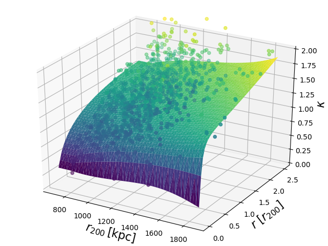
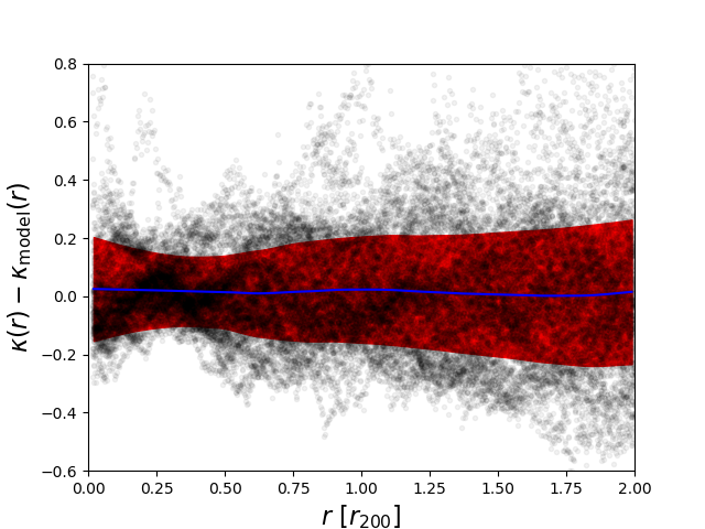
Figure 1: $\kappa$-profiles for the 51 clusters of the RAMSES simulation, as function of radius and $r_{200}$. Left panel shows a 2D smoothing spline to the profiles, and right panel shows the 1$\sigma$ scatter contours of the residuals collapsed along the $r_{200}$ direction. The smoothed surface, and scatter profile serves as parametrization for $\kappa(r,r_{200})$ profiles for observations.

The energy-argument that the DM dispersion should be approximately equal to the gas temperature ($\kappa\approx 1$) in relaxed gravitating structures has a long history (Sarazin, 1986). The anticipation that $\kappa$ may change significantly when gas is cooling was investigated by Hansen et al. (2011), where $\kappa$ was extracted for Milky Way like galaxies as a function of redshift (where cooling is extremely much more significant than in cluster outskirts). There it was found that as long as the high-density/low-temperature component of the gas is removed, then $\kappa$ remains close to unity around $z=0$.

Here we take possibly the most modern approach to gas cooling and other radiative processes in simulation to extract $\kappa$. We chose to use a simulation with the AMR code RAMSES (Teyssier, R., 2002), which uses flat $\Lambda$CDM cosmology with cosmological constant density parameter $\Omega_{\Lambda}=0.728$, matter density parameter $\Omega_{m}=0.272$ of which the baryonic density parameter is $\Omega_{b}=0.045$, power spectrum normalization $\sigma_{8}=0.809$, primordial power spectrum index $n_{s}=0.963$, and current epoch Hubble parameter $H_{0}=70.4\,\mathrm{km}/\mathrm{s}/\mathrm{Mpc}$. To identify large galaxy clusters, the simulation was initially run as a dark-matter-only simulation with comoving box size $144\,\mathrm{Mpc}/h$ and particle mass $m_{\mathrm{DM}}=1.55\cdot 10^{9}\,M_{\odot}/h$. Here $h$ is the dimensionless Hubble parameter, defined as $h=\frac{H_{0}}{100\,\mathrm{km}/\mathrm{s}/\mathrm{Mpc}}$. After running the dark matter only simulation, 51 cluster sized haloes with total masses above $10^{14}\,M_{\odot}/h$ were identified and resimulated including the baryonic component, with dark matter particle mass $m_{\mathrm{DM}}=1.62\cdot 10^{8}\,M_{\odot}/h$ and baryonic component mass resolution of $3.22\cdot 10^{7}\,M_{\odot}$. The 51 resimulation runs implemented models of radiation, gas cooling, star formation, metal enrichment, supernova and AGN feedback, and were evolved to $z=0$. A detailed description of the simulation can be found in Martizzi et al. (2014).

For the 51 clusters, the $\kappa$ profile can be calculated in spherical bins according to equation 6. Since all quantities contained in $\kappa$ depend on the cluster size, we calculate a 2D smoothing spline surface for the 51 $\kappa(r,r_{200})$ profiles, such that given $r_{200}$ for a cluster, $\kappa(r)$ can be retrieved (left panel of figure 1). The error associated with using this $\kappa$ function is approximated from the residual after collapsing it in the $r_{200}$ direction (figure 1 right panel), and we find no strong correlation or systematics within these residuals. The resulting 1$\,\sigma$ standard deviation profile can then be taken into account when estimating $\beta(r)$. When we compare with older numerical techniques, such as the use of GADGET-2 (Kay et al., 2007) (previously used to extract $\kappa$ (Host et al., 2009)), then we find that the resulting $\kappa$ profiles are in fair agreement with each other, within the error-bars.

Herein lies the core of the method, but notably also the reason why resulting $\beta$ profiles cannot be called de facto measurements. Rather they are consistency checks with the DM model employed in the simulation that produces the $\kappa$ relation. The Jeans equation assumes DM to be collisionless, as (in this case) does the simulation that produces $\kappa$, however should this assumption not be valid, a measured $\beta$ profile might not be consistent with those of simulations. From an observational point of view, the $\kappa$-parametrisation makes good sense, as measurements of the mass profile and thus $r_{200}$ of galaxy clusters are independent of $\kappa$. Thus by observing the properties of the hot X-ray emitting gas we can obtain $\kappa(r)$ using our parametrization, and from this calculate $\sigma_{r}^{2}(r)$ from eq. 9 and finally $\beta(r)$ from eq. 8 and 6, assuming that the gas is fully equilibrated. The next section is dedicated to reinforcing the soundness of this assumption in the observations that we choose to analyze.

5 Excluding infeasible sectors from analysis

One of the core assumptions in deriving massprofiles from the X-ray signal in galaxy clusters is that of hydrostatically equilibrated gas. This excludes a large block of potential cluster targets for study, as merging and other irregularities causes a failure to meet this demand. Previous studies show how cluster merging can cause cold front and sloshing in the hot baryonic gas, and phenomena that show up in derived X-ray profiles as unequilibrated features (Markevitch & Vikhlinin, 2007). Data quality has however heightened through the last decades, and so has the frequency of attempts at solving this issue through data selection - considering only sections of the observational plane which best meets the assumptions of equilibrium. This makes sense if material falling onto an equilibrated structure is small enough to only disturb equilibrium locally, or that the in-falling material has not yet had time to perturb the larger equilibrated cluster in its entirety.

In order to develop and test a method of measuring $\beta$ to high radii through data selection in the observational plane of galaxy clusters, we construct a mock observational catalogue from the RAMSES re-simulated clusters. Radial profiles of all quantities relevant for the present work has been extracted. We select a sub-sample of 10 randomly selected clusters in range $14<\log{m_{200}}<15$ where half of the clusters in the sample have been classified as globally relaxed, following the criterion of Martizzi and Agrusa 2016 (Martizzi & Agrusa, 2016). We choose a line of sight through them at random and divided each observational plane of the 10 clusters into 8 equiangular sectors. The motivation for this division originates in the Perseus X-ray observations analyzed in the next sections. Perseus is precisely observed along 8 arms at evenly spaced angles, yielding 8 gas density and temperature profiles in total for the cluster. Previous analysis of the 8 arms of Perseus has shown signatures of cold-fronts and sloshing of the gas in 5 of the 8 arms suggesting that they are suboptimal for calculations assuming hydrostatic equilibrium. The remaining 3 are shown to be more relaxed. In the following we take a similar approach selecting just the sectors that are equilibrated. We conclude that by deselecting the most deviant sectors we can reduce the scatter in our final measurements of $\beta$ within the RAMSES clusters.

For each of the sectors in the observational plane, 3D radial profiles from spherical shells were extracted for the gas and dark matter component, using only the particles that in projection are contained inside of that sector. Each sector can then be analyzed separately, and thus parts of the observed cluster that displays unequilibrated features may be excluded from our calculation of $\beta(r)$. With this in hand, we estimate the statistical reward in removing sectors from analysis, and use this in an attempt to reduce the errorbars of $\beta(r)$ for actual X-ray data.

Figure 2 displays gas temperature and density profiles for 6 of the 10 resimulated galaxy clusters for which we have 3D data. The remaining 4 clusters displayed enough unequilibrated features in the gas component that they were unfit to consider for further analysis, due to strongly inconsistent profiles across the 8 sectors of a cluster, or a steep incline in the central temperature profiles. It should be noted, that only three of the six clusters remaining were categorized as virialized using the criteria of Martizzi & Agrusa (2016). Each column of figure 2 represent one of the six clusters, and the colored profiles represent individual sectors. Top panels show the gas temperature scaled by a constant, and the central panels show the gas density also scaled. From these two quantities alone it is clear that sectors within a single cluster displays some variance, which is natural to expect from a 3D numerical simulation, but also a reflection of the hydrostatic equilibrium assumption not being perfectly true. For the remainder of this section we will discuss which directions appear less equilibrated than others, considering purely the observational gas profiles.

For some of the clusters, looking only at the top two rows of figure 2 it is not always easy to tell whether parts of the cluster are effected by some disturbing element. The 5th column has a pretty clear signature in the temperature profiles that something is disturbing its equilibrium in the dark blue, purple and pink sectors. For the cluster in the 6th column, deviations from hydrostatic equilibrium are more subtle. Herein lies an observational challenge, and in an attempt to enhance the visibility of such subtle differences between sectors within a single galaxy cluster, we combine the two measurable quantities $\rho_{\mathrm{gas}}$ and $T_{\mathrm{gas}}$ into a single measure.

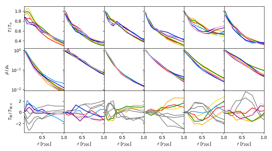
Figure 2: Temperature profiles (top row), gas density profiles (middle row) and weighted temperature variation profiles (bottom row) for the six resimulated RAMSES clusters considered for analysis. Each color represents one of the 8 sectors within the cluster. Neighbouring sectors are colored in the following order: Red, orange, yellow, green, light blue, dark blue, purple, pink. The gray profiles in the bottom row indicates the sectors that were excluded from analysis due to their profile as discussed in the main text. Note that $T$, $\rho$ and $T_{W}$ profiles are scaled by a constant $T_{\mathrm{n}}$, $\rho_{\mathrm{n}}$ and $T_{\mathrm{W,n}}$, which differs within each cluster, in order to compare profile shapes between clusters in this figure.

The bottom panels of figure 2 show this combination in the form of a weighted temperature variation profile,

$$T_{\mathrm{W}}=\rho_{\mathrm{gas}}r^{2}\left(1-\frac{T_{\mathrm{gas}}}{\overline{T_{\mathrm{gas}}}}\right),$$ (11)

where $\overline{T_{\mathrm{gas}}}$ is the mean temperature profile of the entire cluster. This observationally available construct emphasizes in some cases distinct groups of sectors, and by comparing these to the gas and temperature profiles of the same cluster, we try to deselect those that are least consistent with the overall trend of the cluster. Here bumps i.e. cold fronts in the temperature and density profile are features we look for (Markevitch & Vikhlinin, 2007). In the case of well behaved clusters, this of course is less obvious, and arguably data selection may also have less of an effect. In column 3 of figure 2 the density is smooth, but the dark blue, light blue, pink, purple and red directions have a bump in the temperature profile. The $T_{\mathrm{W}}$ profiles show two groups that clearly differ from each other. Based on the irregular bump in the $T_{\mathrm{gas}}$ profile and the separation in the $T_{\mathrm{W}}$ figure we include only the green, orange and yellow directions, and indicate the deselected sectors with the grey color in the bottom panel. In column 6 the two blue sectors stand out slightly in the $T_{\mathrm{gas}}$-profile, but more profoundly in the $T_{\mathrm{W}}$ profile, and are thus removed from analysis. Column 2 displays a very smooth cluster, and it is less clear which (if any) directions should be removed. We deselect the green, yellow and orange directions as they tend to lie slightly high for the high radii of primary interest for this paper. The cluster in the first column shows a kink towards its inner parts. Here, the red, orange, green and yellow profiles deviate largely within 0.7$r_{200}$ from the remaining four sectors, and are thus removed from analysis. The $T_{\mathrm{W}}$ profiles of column 4 shows three main groups, substantiating what is otherwise hard to see in the $T_{\mathrm{gas}}$ profiles alone. We remove from analysis the dark blue, light blue, purple and pink and keep the most coherent 4 sectors as indicated in the figure.

In some clusters, such as the one in column 5 of figure 2, signatures of a ”cold-front” is visible in the sectors represented by the dark-blue, pink and purple profiles, which are consequently removed from analysis. These may be caught by performing an analysis of the X-ray data analogous with the one in Urban et al. (2014), and in this case both approaches would possibly single out the same sectors. The present exclusion process however singles out some features that are not predominantly cold-front related, and as such provides a different approach to determining which parts of a galaxy cluster that are not in equilibrium.

From the weighted temperature variation profiles in combination with the raw density and temperature profile, we have identified up to five sectors within each cluster that deviate substantially from the more relaxed conditions, and are now ready to calculate the velocity anisotropy parameter $\beta$.

6 Non-parametric fitting and MC resampling to data

In order to arrive at an estimate of $\beta$, local fluctuations and measurement uncertainties are necessary to take into account. We employ non-parametric locally estimated scatter plot smoothing (LOESS) fitting to the gas density and temperature measurements in order to smooth out local variations (Scrucca, 2011). In this way we manage to avoid imposing an analytical profile to our data. This yields a fitted curve and a 1$\sigma$ standard deviation profile in addition. Any fit, including this one, is of course subject to a level of arbitrarity in the choice of function, and for non-parametric fits some choice of smoothing parameter and algorithm. In this case, we let the LOESS smoothing parameter be determined by a generalized cross-validation technique (Wang, 2010), which adapts to the data in question. Doing this, we obtain a smooth profile, that neglects local bumps and wiggles, however allows for larger scale variation, rather than forcing it to follow a strict parametric form. An example of a cross-validated LOESS fit to the gas temperature profile is seen is seen in figure 3 for a single sector in one of the galaxy clusters within the RAMSES simulation. In this example the temperature profile from the simulated data is without uncertainty and smooth in comparison with realistic measurements of the 3D temperature profiles of galaxy clusters. Therefore Gaussian errors of $3\times 10^{6}\,$K and error bars of the same magnitude are added. The red band of figure 3 represents the 68% percentile of 100 LOESS fit to the noisy data using a resampling technique assuming a Gaussian distribution, and recreates the original temperature profile in black reasonably well. The same goes for the $\rho_{\mathrm{gas}}$ in the bottom panel, though this is to be expected as uncertainties in typical gas density profiles are small compared to the temperature measurements. As explained in section 7 we employ a Monte Carlo resampling approach to obtain error estimates on the measurement of the galaxy cluster $\beta$. For an input smoothed $T_{\mathrm{gas}}$ and $\rho_{\mathrm{gas}}$ we proceed to calculate $M(r)$, $\sigma_{r}^{2}(r)$ and $\beta(r)$ through hydrostatic equilibrium assumptions, as shown in section 2. In this process, we fit yet another LOESS curve to both the $M(r)$, $\rho$ and $\sigma_{r}^{2}(r)$ profiles, to neglect the smaller bumps and ripples. This comprises the drawback of not assuming and fitting e.g. well behaved power law functions to the raw hydrostatic data. However, the multiple non-parametric fits do allow a degree (as controlled by the cross-validation mentioned above) of ripple that would otherwise not be seen in the parametric form, and in this respect the approach is arguably preferable. In the next section we can begin the process of Monte Carlo resampling $\rho_{\mathrm{gas}}$, $T_{\mathrm{gas}}$ and $\kappa$ to arrive at a final estimate of $\beta$ and its uncertainty from a number of sectors within a single galaxy cluster.

7 Errors in estimating $\beta$

Each sector of each cluster is handled individually in our analysis. The final $\beta$ of a given sector is obtained using a Monte Carlo resampling approach, which allows us to propagate measurement errors from the input X-ray profiles. For a single sector we produce a number $N_{\mathrm{MC}}$ of resamples of $T_{\mathrm{gas}}(r)$ using its measurement uncertainties. We resample complementary $\kappa(r)$ profiles and proceed to calculate $M(r)$, $\sigma_{r}^{2}(r)$ and $\beta(r)$ through hydrostatic equilibrium assumptions, as shown in section 2 and 6. The final $\beta$ profile for a given sector is then the median profile of all $\beta$ from the resamples of that sector. Our intent is to use the procedure on multiple sectors of a single cluster (or potentially even multiple clusters, though this is left for future work), and end up with a final estimate of the universal velocity anisotropy profile. We must therefore understand to what degree the procedure is biased, and how much scatter it introduces in addition to the natural scatter within cluster $\beta$ profiles. To do this, we measure the $\beta$ profile of two groups of sectors from the 6 RAMSES clusters selected in section 5: One group consisting of all 48 sectors in the 6 RAMSES clusters, and another group using only the 27 equilibrated sectors. Starting with the full set, as an intermediary step the hydrostatic massprofiles of each sector is calculated. These can be seen in figure 4, relative to the true mass profiles. The hydrostatic masses are just within the 1$\sigma$ standard deviation profile at the radii of interest, however the mean value under-performs between between 0 and 10% low for growing radii similar to previous findings using other mass reconstruction techniques (Gifford & Miller, 2013; Armitage et al., 2018). One could imagine correcting inferred masses accordingly upon measurements, however it is non-trivial how that translates into a $\beta$ correction given the simulated data we have available. For this reason we allow the hydrostatic mass measurements to under perform at these radii. Proceeding towards $\beta$, figure 5 on the left shows in the red curve and red band a LOESS fit and $\sigma$ scatter of the true $\beta$ profiles for the full set of sectors. The black curve and grey band shows the same, but for the $\beta$ profiles as measured by only the gas observables of each sector. The mock measurement of $\beta$ in a sector is seen to be unbiased, with a scatter determined largely by the true scatter in $\beta$ until around 0.5$\,r_{200}$, at which point the scatter is dominated by assumptions of equilibrium breaking down. In order to lessen the scatter, only the sectors selected in section 5 i.e. the second set of sectors was used, and their true and measured $\beta$ summarized in the right hand side of figure 5. Notably, the scatter is lower in this case because assumptions of equilibrium are better met in these selected simulated sectors. The grey patches in the right panel of figure 5 comprises scatter in the true $\beta$ profiles of the simulated clusters, as well as additional scatter introduced by our analysis. As we proceed to calculate $\beta$ for X-ray observations of the sectors in a single real galaxy cluster, we must incorporate this scatter in the uncertainty of our measurement. How this is done depends on the amount of correlation between sectors of a single galaxy cluster. If all sectors within a single cluster are completely independent measurements of $\beta$, then the uncertainty of the joint $\beta$ profile decreases by a factor $1/\sqrt{N}$ where $N$ is the number of sectors under analysis. If on the other hand sectors within a single cluster are completely correlated, the part of the scatter that originates from natural variation in $\beta$ (red patch of figure 5) is constant with number of sectors, whereas the residual scatter (difference between grey and red scatter) in figure 5, i.e. the additional scatter introduced by the analysis framework is reduced by $1/\sqrt{N}$, assuming that the two sources of scatter are directly separable. As one extreme, we could assume that all of the sectors of a single galaxy were uncorrelated in their measurement of $\beta$, and as another we could assume complete correlation. Now we have an estimate of the uncertainties involved in measuring $\beta(r)$ through X-ray data and assumptions of hydrostatic equilibrium, and a method for eliminating parts of this uncertainty by data selection. In the next section we move to apply the technique and estimate $\beta(r)$ to the virial radius for the Perseus galaxy cluster.

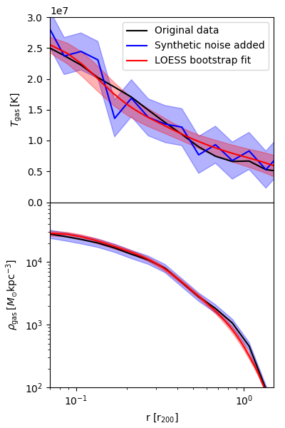
Figure 3: Example of the temperature (upper panel) and density (lower panel) LOESS fits employed in the hydrostatic equilibrium calculation for the gas component, as applied to a single sector from one of the simulated clusters. Top panel shows $T_{\mathrm{gas}}$ and bottom panel $\rho_{\mathrm{gas}}$. Black lines show the original profiles. The blue curves and patches shows the profile with synthetic noise and errorbars added, and the red curves shows the median and 68% percentile of 100 bootstrap resampled Monte Carlo LOESS fits to the noisy profiles.

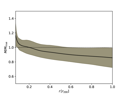
Figure 4: The mass profiles from hydrostatic equilibrium for all sectors of the 6 RAMSES clusters relative to the true mass profile of the cluster they belong to. The black curve represents a LOESS fit to the individual profiles, and the grey band represents the 1$\,\sigma$ standard deviation of the profiles, as obtained from the generalized cross-validation technique of the LOESS fit outlined in the main text.

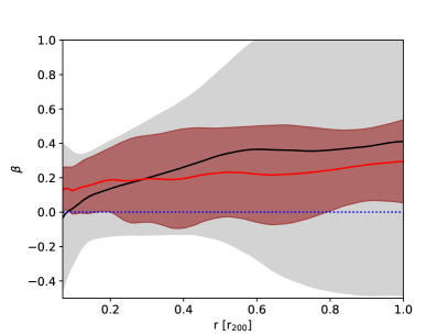
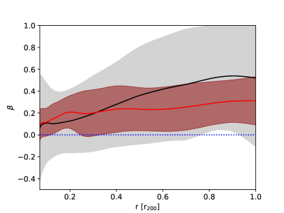
Figure 5: $\beta$ profile for all sectors (left) and selected sectors (right) for the six relaxed RAMSES clusters using interpolated 2D smoothing spline $\kappa$-profiles for each cluster. Red curve shows a LOESS fit to the true $\beta$-profiles, and black curves to measured ones. The red narrow patches indicate the 1$\sigma$ standard deviation of the true $\beta$-profiles, and the light grey wider patches indicated the same but for the measured $\beta$-profiles, as obtained through the generalized cross validation technique of the LOESS fit outlined in the main text. Thus the standard deviations shown here is for a single sector of a single cluster.

8 Perseus cluster observations in X-ray

The Perseus cluster is the brightest cluster in the X-ray sky, and was observed in 85 pointings as a Suzaku Key Project, with a total exposure time of 1.1 Ms. The low particle background makes Suzaku ideal for analysing cluster outskirts. These pointings were arranged in eight arms along different azimuthal directions. For each direction the data had point sources removed and was cleaned, 21 pointings were used for a careful background modelling, and XSPEC was used to extract the deprojected temperature and density profiles (Simionescu et al., 2011; Urban et al., 2014). Such careful treatment of the deprojection is necessary, as the calculation of $\beta$ requires 3D profiles of $T_{\mathrm{gas}}$ and $\rho_{\mathrm{gas}}$ to function. For each of the eight arms, the $T_{\mathrm{gas}}$ and $\rho_{\mathrm{gas}}$ profiles can be seen with uncertainties in the top and middle panel of the LHS column in figure 6.

Previous careful analyses allowed a categorization of the eight arms into three “relaxed” arms showing no particular irregular behaviour, where in particular the temperature profiles are generally decreasing functions of radius. The other arms either show signs of large cold fronts between 20 and 50 arcminutes form the center, or showed signs of large scale sloshing motion of the gas (Simionescu et al., 2011, 2012; Urban et al., 2014).

In this work, we consider temperature variations relative to the mean profile, and weigh them by $\rho r^{2}$ as described in equation 11. The $T_{\mathrm{W}}$ profiles are seen in the bottom panel of the first column in figure 6. Since Perseus is already a comparatively virialised cluster, there are not a couple of sectors that show extremely obvious deviant features from the mean temperature profile. The western arm (magenta) shares more or less no features with the rest, and is arguably not in equilibrium with the remaining parts of the cluster. Beyond 0.7$\,r_{200}$ the spread of the profiles becomes very large and the profiles deviate significantly from each other. Within 0.7$\,r_{200}$ the Eastern (black), North Eastern (red) and to a lesser extent the South Eastern (brown) arms display an irregularity that Urban et. al conclude to be a cold front. Here we shall remove Eastern and North Eastern arms, the ones furthest from the mean temperature profile below 0.5$r_{200}$ and with a general downwards tendency beyond $r_{200}$ in the $T_{\mathrm{W}}$ profiles (figure 6 bottom row central column). Instead we focus on the remaining 5 profiles closer to the mean below $r_{200}$ and with the upwards tendency in the $T_{\mathrm{W}}$ profiles beyond $r_{200}$ (figure 6 bottom row 3rd column). Then we are consistent with the methodology of the previous sections, where the numerical clusters were considered, and arrive at the selections in the 3rd column of figure 6. The middle column shows the profiles that are not included in the analysis.

This leaves us with three sets of data within Perseus: The full set, the sectors selected here and the ones found to be relaxed by previous analysis (Urban et al., 2014). In the following section we examine all three sets. Each arm is fed through our analysis separately, and in the end we stack the $\beta$ of each set to obtain an overall estimate of $\beta$ from Perseus.

We do not consider radii outside the virial radius, where the infall motion leads to departure from hydrostatic equilibrium (Falco et al., 2013; Albæk et al., 2017).

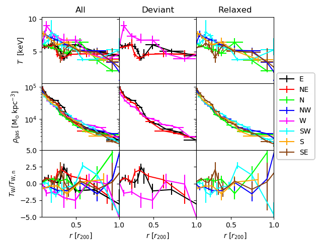
Figure 6: Deprojected profiles for the 8 sectors of the Perseus cluster, grouped in categories through columns "All", "Deviant" and "Relaxed". Top row shows the gas temperature $T_{\mathrm{gas}}$, center row the gas density $\rho_{\mathrm{gas}}$ and bottom row the weighted temperature variation $T_{\mathrm{W}}$.

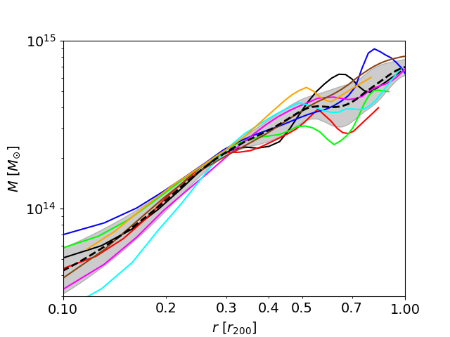
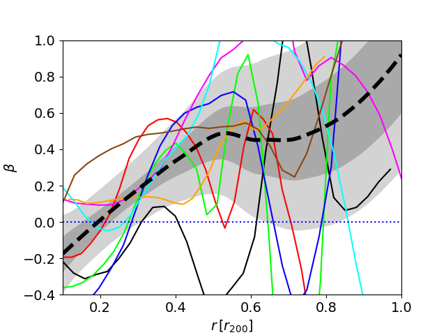
Figure 7: Left: Mass profiles for the 8 sectors of Perseus as obtained from hydrostatic equilibrium. Gray band shows the 1$\sigma$ spread of the individual profiles. Note the logarithmic $r$-axis. Right: Calculated $\beta(r)$ profiles for the same directions arms. Dark grey band represents the uncertainty of the mean $\beta$ profile based on the spread of the Perseus sample ($\frac{\sigma}{\sqrt{N}}$ where $N$ is number of sectors), and and light grey is the added uncertainty of the mean based on the standard deviation of the RAMSES full set i.e. the grey area of the LHS panel of figure 5.

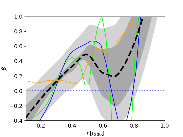
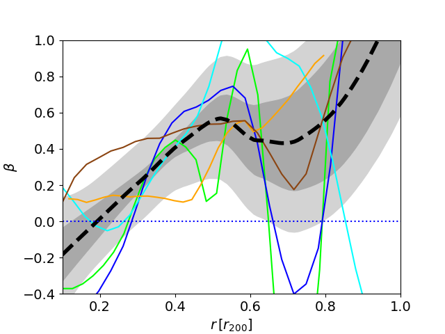
Figure 8: Left: $\beta(r)$ using only the selected 3 sectors which are classified as “Relaxed” in (Urban et al., 2014). Right: $\beta(r)$ using the 5 equilibrated sectors according to section 8 above. In both figures, the black dashed curve shows LOESS fit to the profiles. The dark grey inner band shows the uncertainty of the mean $\frac{\sigma}{\sqrt{N}}$, where $\sigma$ is the spread as obtained through LOESS generalized cross validation, and $N$ is the number of sectors included. The light grey outer band shows the added uncertainty from spread of the RHS of figure 5, i.e. the uncertainty from the measuring technique itself. For each sector, multiple $\beta$ profiles are calculated via the analytical framework and MC bootstrap procedure described in the paper. Slight variations upon each MC realisation occurs, and so the profiles may be slightly different between realisations.

9 Extracting the DM velocity anisotropy in Perseus

Having prepared a method for data selection in the previous sections, and determined 3 sets of sectors for the Perseus cluster to investigate, we are now ready to extract $\beta$ from it. We use the deprojected observations of $T_{\mathrm{gas}}$ and $\rho_{\mathrm{gas}}$ profiles and their corresponding error-bars to perform a Monte Carlo sampling as input for the analysis for each sector i.e. each arm. First $\frac{\partial{\rm ln}\rho_{\mathrm{gas}}}{\partial{\rm ln}r}$ and $\frac{\partial lnT_{\mathrm{gas}}}{\partial{\rm ln}r}$ are found at each radial point by computing central differences in the interior and first differences at the boundaries. These are then used in the hydrostatic equilibrium equation to calculate the mass profile. This mass profile is again subjected to a non-parametric LOESS fit in order to smooth out bumps and wiggles. After subtracting the gas mass, we can directly generate the DM density profile. The resulting mass profile of Perseus can be seen in figure 7 using the data from all 8 arms. For each Monte Carlo sampling a DM temperature profile is also resampled based on the smoothing spline $\kappa$ surface and errors of figure 1, and the resampled gas temperature profile. The $\sigma^{2}_{r}(r)$ profiles can now be calculated for each sample, and hence the $\beta(r)$ profiles.

The results are shown in the bottom panel of figure 7 for all 8 arms of Perseus i.e. the full set. The coloured curves represents the $\beta(r)$ median Monte Carlo profiles obtained from the individual sectors of the Perseus data, and the black dashed curve shows another LOESS smoothing to these curves to estimate an overall $\beta$ for the data included. The inner dark grey band shows the 1$\sigma$ standard error of the mean as obtained via the standard deviation of the LOESS fit, and the light grey outer bands the additional 1$\sigma$ standard error of the mean from of the standard deviation of the $\beta$ obtained from the RAMSES mock data as seen in the left side of figure 5. We see that the the $\beta$ profile ranges from 0 in the inner parts towards 1 at $r_{200}$ where uncertainty grows large on the data and the validity of our assumptions, and thus on $\beta$.

For the partial sets, we perform the same analysis but include only the 3 sectors of the Urban et. al. set, and the 5 sectors selected through $T_{\mathrm{W}}$ profiles. The $\beta$ can be seen in the left and right panel of figure 8 respectively. Here, the grey inner bands represent the same as for the full set, but the outer light grey bands are instead taken from the standard deviation of the right hand side panel of figure 5. We see especially for the set chosen here that $\beta$ is different from 0 between 0.3$r_{200}$ and 0.6$r_{200}$ beyond its standard error. Including all the error-bars, we have here found indications that the velocity anisotropy in Perseus is of the order

$$\beta_{r=0.5r_{200}}=0.5\pm 0.1\pm 0.2\,,$$ (12)

where the error-bars are from: variations within the Perseus cluster sectors, and the added scatter from the hydrostatic equilibrium technique itself as applied on each individual arm. This takes the optimistic stand that sectors within a galaxy cluster are completely uncorrelated measurements of $\beta$. Taking the more pessimistic viewpoint that sectors within a single cluster are completely correlated yields $\beta_{r=0.5r_{200}}=0.5\pm 0.1\pm 0.3$. This includes uncertainty from temperature measurements and uncertainty in $\kappa$. From around 0.6$\,r_{200}$ and up to 0.8$r_{200}$ the estimate of $\beta$ is consistent with 0, and beyond that the error grows as the assumptions of hydrostatic equilibrium breaks down even for the selected clusters and sectors within them. This in fact is already seen in the measured massprofiles of the RAMSES clusters, where the hydrostatic method has large errorbars at these large radii. Generally $\beta$ tends to increase with increasing radius. At $r<0.2r_{200}$ the results are statistically consistent with $\beta=0$, but if the decrease extends to lower radii, it could be interpreted as an effect of the brightest central galaxy making orbits more tangentially biased. However, this effect should not be visible at the scales examined in this work (Host & Hansen, 2011). Figure 10 compares the Perseus estimate to the $\beta$ profile of the chosen sectors of the RAMSES clusters, and again we see, for this single Perseus estimate, that observation and simulation agrees within $r_{200}$.

It is worth keeping in mind that $\beta$ in principle could take on any value between $+1$ and $-\infty$. The simulated values of $\beta$ from these 51 RAMSES clusters are about 0.25 at $r=0.5r_{200}$ (with a 1$\sigma$ spread about 0.2 among the 51 clusters), and at $r\sim r_{200}$ it is about 0.35 (with a dispersion about ${}^{+0.2}_{-0.4}$). Upon comparing the measured $\beta$ with the $\beta$ of the simulated clusters in figure 5 and figure 8 respectively we see that they are in reasonable agreement at least until 0.7$r_{200}$. Another way to visualize the velocity anisotropy parameter is through joining $\sigma_{r}^{2}$ and $\sigma_{t}^{2}$ in the construct

$$\beta_{j}=\frac{\sigma_{r}^{2}-\sigma_{t}^{2}}{\sigma_{r}^{2}+\sigma_{t}^{2}}=\frac{\beta}{2-\beta},$$ (13)

which ranges from -1 to 1. Figure 9 shows precisely this quantity for the 5 sectors of the Perseus cluster selected here, where the $\beta_{j}$ profile with its standard error of the mean is seen to be non-trivial below 0.6$r_{200}$.

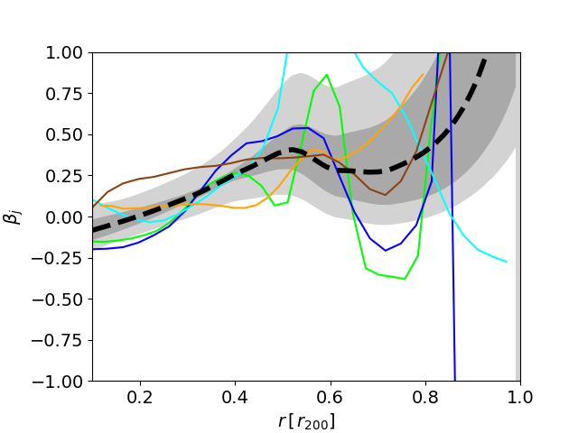
Figure 9: The non-standard and symmetrized $\beta_{j}$, which can only assume values between $-1$ and $+1$, plotted for the 5 sectors of Perseus selected in the present work through $T_{\mathrm{W}}$. The black dashed line shows the LOESS fit to the five profiles. The inner and outer grey bands are the standard errors of the mean similarly to the ones of figure 7.

It should be noted, that in spite of removing data from the analysis, the Perseus resulting $\beta$ is comparable to that of the one with the full data both in terms of the mean curve and the error. Perseus is itself a virialized cluster, and thus expectations of bettering the beta estimate remarkably with this data selection technique are low. However, as multiple clusters are discovered and analyzed through the same technique, our results from the RAMSES simulation show that it is possible to better the uncertainty in $\beta$ measurements by conducting data selection of the type outlined here. Høst et al. obtained estimates of $\beta$ within $r_{2500}$ for a stack of 16 clusters observed in X-ray (Host et al., 2009), whereas here we analyze just one single cluster. In the future we hope to include future cluster X-ray observations to high radii to further bring uncertainties down.

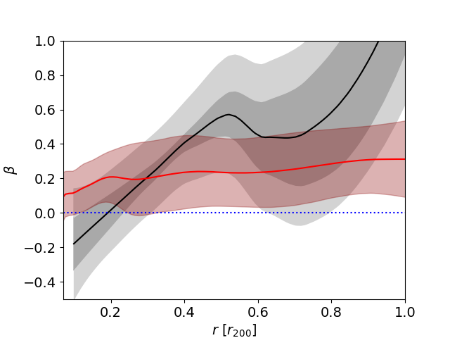
Figure 10: Comparison of the true $\beta$ profile from RAMSES (red curve) and the estimated $\beta$ profile for Perseus (black curve). The RAMSES profile is comprised of the $\beta$ profiles of the relaxed sectors of the relaxed clusters as also shown in the RHS panel of figure 5. The Perseus profile is the same as shown in the bottom panel of figure 8 for the 5 arms selected through our analysis. Again the dark grey inner band shows the uncertainty of the mean $\frac{\sigma}{\sqrt{N}}$, where $\sigma$ is the standard deviation as obtained through LOESS generalized cross validation, and $N$ is the number of sectors included. The light grey outer band shows the added uncertainty from spread of the RHS of figure 5, i.e. the uncertainty from the measuring technique itself.

10 Conclusion

The dark matter velocity anisotropy contains information on the dynamics of dark matter in equilibrated structures. By combining the gas equation from hydrostatic equilibrium and the DM equation i.e. the Jeans equation with input from a numerical cosmological simulation that includes the baryonic component, we are able to test the consistency of the velocity anisotropy measure for Perseus with the dark matter model employed in this simulation. We find that the velocity anisotropy of Perseus is consistent with that of the cosmological model employing a $\Lambda$CDM cosmology, lending support to the cold and collisionless nature of DM in galaxy clusters. Our analysis of the Perseus data agrees with previous estimates on the velocity anisotropy. Previous studies employ the strength of a catalogue of 16 galaxy clusters. However, since deprojected gas profiles are requirement of the analysis the results were within 0.85$\,r_{2500}$. The quality and radial extent of the Perseus data allows us to probe the consistency of the DM model towards the virial radius. By analyzing and including only sectors of the cluster that displays a well behaved radial X-ray signal, we show that we in simulation are able to put better constraints on the velocity anisotropy estimates, however for Perseus we are only able to get meaningful constraints towards 0.6$r_{200}$, which is still a large improvement of about a factor of 3 compared to previous work.

The method comes with some caveats: A relation $\kappa$ from numerical simulations between the gas temperature and the dark matter total velocity dispersion i.e. the “DM temperature” is used to calibrate the measurement of the velocity anisotropy. The velocity anisotropy measure of a galaxy cluster in observation is only ever as good as the $\kappa$ that it is calibrated against. Since we assume a DM model in all cosmological simulations we at best are able to measure velocity anisotropy as relying on the assumptions of the simulation. Therefore, our velocity anisotropy measurement should be viewed as a check of consistency with the model employed in the estimation of the total DM velocity dispersion. Furthermore, the Perseus data comprises just a single galaxy cluster. To obtain better constraints on the velocity anisotropy measure is a statistical challenge, and even a couple of galaxy cluster data sets of the same quality would strengthen the analysis greatly.

Our final remarks concern future analyses. Above we have made the assumption of hydrostatic equilibrium. It is well known that departure from hydrostatic equilibrium impacts the mass determinations, see e.g. Nelson et al. (2014) for a list of references, and also that the velocity anisotropy directly or through mass profiles may depend on orientation (Sparre & Hansen, 2012; Wojtak et al., 2013; Svensmark et al., 2015). We also assume sphericity of the cluster which have previously been found to impact mass estimates of clusters. Perseus was chosen because it does have a relaxed appearance, and we have chosen only the 5 most relaxed arms. Furthermore, at the moment the large scatter in $\kappa$ leads to large error-bars of $\beta$. By analysing cones in numerical simulated clusters, for instance separating according to differences in temperature profiles such as cool-core (CC) and non-CC cones, one might be able to reduce scatter in $\kappa$, and hence obtain smaller error-bars of the DM $\beta$.

Few alternative methods to estimate the DM velocity anisotropy exits (Lemze et al., 2012; Mamon et al., 2013). Future analyses which would improve on the method discussed here, could be forced to attempt to improve on the mass determination by including complementary observation e.g. from lensing or the SZ effect (Kneib & Natarajan, 1996; Stark et al., 2017). Here one will, however, have to deal with the difficult systematic effects when combining such different observational techniques.

References

- ATLAS Collaboration et al. (2015) ATLAS Collaboration Aad G., Abbott B., Abdallah J., Abdel Khalek S., 2015, The European Physical Journal C, 75, 92
- Agnes et al. (2015) Agnes P., et al., 2015, Physics Letters B, 743, 456
- Albæk et al. (2017) Albæk L., Hansen S. H., Martizzi D., Moore B., Teyssier R., 2017, Monthly Notices of the Royal Astronomical Society, 472, 3486
- Amorisco et al. (2014) Amorisco N. C., Zavala J., de Boer T. J. L., 2014, The Astrophysical Journal Letters, 782, L39
- Armitage et al. (2018) Armitage T. J., Kay S. T., Barnes D. J., Bahé Y. M., Dalla Vecchia C., 2018, Monthly Notices of the Royal Astronomical Society, 482, 3308
- Benitez-Llambay et al. (2018) Benitez-Llambay A., Frenk C. S., Ludlow A. D., Navarro J. F., 2018, arXiv e-prints, p. arXiv:1810.04186
- Binney & Tremaine (2008) Binney J., Tremaine S., 2008, Galactic Dynamics: Second Edition. Princeton University Press
- Bœhm et al. (2002) Bœhm C., Riazuelo A., Hansen S. H., Schaeffer R., 2002, Phys. Rev. D, 66, 083505
- Bose et al. (2018) Bose S., et al., 2018, arXiv e-prints, p. arXiv:1810.03635
- Brinckmann et al. (2018) Brinckmann T., Zavala J., Rapetti D., Hansen S. H., Vogelsberger M., 2018, Monthly Notices of the Royal Astronomical Society, 474, 746
- Bullock et al. (2015) Bullock J. S., Oñorbe J., Boylan-Kolchin M., Hopkins P. F., Kereš D., Faucher-Giguère C.-A., Quataert E., Murray N., 2015, Monthly Notices of the Royal Astronomical Society, 454, 2092
- Clowe et al. (2006) Clowe D., Bradač M., Gonzalez A. H., Markevitch M., Randall S. W., Jones C., Zaritsky D., 2006, The Astrophysical Journal Letters, 648, L109
- Di Cintio et al. (2017) Di Cintio A., Tremmel M., Governato F., Pontzen A., Zavala J., Bastidas Fry A., Brooks A., Vogelsberger M., 2017, Monthly Notices of the Royal Astronomical Society, 469, 2845
- Dutton et al. (2018) Dutton A. A., Macciò A. V., Buck T., Dixon K. L., Blank M., Obreja A., 2018, arXiv e-prints, p. arXiv:1811.10625
- Faham (2014) Faham C., 2014, preprint, (arXiv:1405.5906)
- Falco et al. (2013) Falco M., Mamon G. A., Wojtak R., Hansen S. H., Gottlöber S., 2013, Monthly Notices of the Royal Astronomical Society, 436, 2639
- Fitts et al. (2018) Fitts A., et al., 2018, arXiv e-prints, p. arXiv:1811.11791
- Gifford & Miller (2013) Gifford D., Miller C. J., 2013, The Astrophysical Journal, 768, L32
- Gilmore et al. (2007) Gilmore G., Wilkinson M. I., Wyse R. F. G., Kleyna J. T., Koch A., Evans N. W., Grebel E. K., 2007, The Astrophysical Journal, 663, 948
- González-Samaniego et al. (2017) González-Samaniego A., et al., 2017, Monthly Notices of the Royal Astronomical Society, 472, 2945
- Hansen (2009) Hansen S. H., 2009, The Astrophysical Journal, 694, 1250
- Hansen, S. H. & Piffaretti, R. (2007) Hansen, S. H. Piffaretti, R. 2007, A&A, 476, L37
- Hansen et al. (2011) Hansen S. H., Macció A. V., Romano-Diaz E., Hoffman Y., Brüggen M., Scannapieco E., Stinson G. S., 2011, The Astrophysical Journal, 734, 62
- Hinshaw et al. (2013) Hinshaw G., et al., 2013, The Astrophysical Journal Supplement Series, 208, 19
- Host & Hansen (2011) Host O., Hansen S. H., 2011, The Astrophysical Journal, 736, 52
- Host et al. (2009) Host O., Hansen S. H., Piffaretti R., Morandi A., Ettori S., Kay S. T., Valdarnini R., 2009, The Astrophysical Journal, 690, 358
- Kay et al. (2007) Kay S. T., Da Silva A. C., Aghanim N., Blanchard A., Liddle A. R., Puget J.-L., Sadat R., Thomas P. A., 2007, Monthly Notices of the Royal Astronomical Society, 377, 317
- Kneib & Natarajan (1996) Kneib J.-P., Natarajan P., 1996, Monthly Notices of the Royal Astronomical Society, 283, 1031
- Lemze et al. (2012) Lemze D., et al., 2012, The Astrophysical Journal, 752, 141
- Liu et al. (2016) Liu H., Slatyer T. R., Zavala J., 2016, Phys. Rev. D, 94, 063507
- Lowette & for the CMS Collaboration (2014) Lowette S., for the CMS Collaboration 2014, preprint, (arXiv:1410.3762)
- Mamon et al. (2013) Mamon G. A., Boué G., Biviano A., 2013, Monthly Notices of the Royal Astronomical Society, 429, 3079
- Markevitch & Vikhlinin (2007) Markevitch M., Vikhlinin A., 2007, Physics Reports, 443, 1
- Martizzi & Agrusa (2016) Martizzi D., Agrusa H., 2016, arXiv e-prints, p. arXiv:1608.04388
- Martizzi et al. (2014) Martizzi D., Mohammed I., Teyssier R., Moore B., 2014, Monthly Notices of the Royal Astronomical Society, 440, 2290
- Navarro et al. (2010) Navarro J. F., et al., 2010, Monthly Notices of the Royal Astronomical Society, 402, 21
- Nelson et al. (2014) Nelson K., Lau E. T., Nagai D., 2014, The Astrophysical Journal, 792, 25
- Planck Collaboration et al. (2018) Planck Collaboration et al., 2018, arXiv e-prints, p. arXiv:1807.06209
- Pointecouteau, E. et al. (2005) Pointecouteau, E. Arnaud, M. Pratt, G. W. 2005, A&A, 435, 1
- Salucci et al. (2007) Salucci P., Lapi A., Tonini C., Gentile G., Yegorova I., Klein U., 2007, Monthly Notices of the Royal Astronomical Society, 378, 41
- Santos-Santos et al. (2017) Santos-Santos I. M., Di Cintio A., Brook C. B., Macciò A., Dutton A., Domínguez-Tenreiro R., 2017, Monthly Notices of the Royal Astronomical Society, 473, 4392
- Sarazin (1986) Sarazin C. L., 1986, Rev. Mod. Phys., 58, 1
- Scrucca (2011) Scrucca L., 2011, Computational Statistics & Data Analysis, 5, 3010
- Simionescu et al. (2011) Simionescu A., et al., 2011, Science, 331, 1576
- Simionescu et al. (2012) Simionescu A., et al., 2012, The Astrophysical Journal, 757, 182
- Sparre & Hansen (2012) Sparre M., Hansen S. H., 2012, Journal of Cosmology and Astroparticle Physics, 2012, 042
- Stark et al. (2017) Stark A., Miller C. J., Halenka V., 2017, arXiv e-prints, p. arXiv:1711.10018
- Svensmark et al. (2015) Svensmark J., Hansen S. H., Wojtak R., 2015, Monthly Notices of the Royal Astronomical Society, 448, 1644
- Teyssier, R. (2002) Teyssier, R. 2002, A&A, 385, 337
- Teyssier et al. (2013) Teyssier R., Pontzen A., Dubois Y., Read J. I., 2013, Monthly Notices of the Royal Astronomical Society, 429, 3068
- Urban et al. (2014) Urban O., et al., 2014, Monthly Notices of the Royal Astronomical Society, 437, 3939
- Vikhlinin et al. (2006) Vikhlinin A., Kravtsov A., Forman W., Jones C., Markevitch M., Murray S. S., Speybroeck L. V., 2006, The Astrophysical Journal, 640, 691
- Wang (2010) Wang X.-F., 2010, fANCOVA: Nonparametric Analysis of Covariance. https://CRAN.R-project.org/package=fANCOVA
- Wetzel et al. (2016) Wetzel A. R., Hopkins P. F., hoon Kim J., Faucher-Giguère C.-A., Kereš D., Quataert E., 2016, The Astrophysical Journal, 827, L23
- Wheeler et al. (2018) Wheeler C., et al., 2018, arXiv e-prints, p. arXiv:1812.02749
- Wojtak et al. (2013) Wojtak R., Gottlöber S., Klypin A., 2013, Monthly Notices of the Royal Astronomical Society, 434, 1576
- Zavala et al. (2013) Zavala J., Vogelsberger M., Walker M. G., 2013, Monthly Notices of the Royal Astronomical Society: Letters, 431, L20