Twist-three contributions to Charged Current Deeply Virtual Meson production (CCDVMP)

$\rho$- vs . $\pi$-production in Charged Current Deeply Virtual Meson production (CCDVMP)

What studies DVMP: nucleon GPDs or meson DAs ?

Model-independent tests of meson DAs from DVMP

Generalized Parton Distributions from charged current meson production

Abstract

In this paper we prove that the simultaneous study of both $\rho$- and $\pi$-meson production by charged currents in Bjorken kinematics allows for a very clean extraction of the leading twist Generalized Parton Distributions of the target, with inherent control of the contribution of higher-twist corrections. Also, it might provide target-independent constraints on the distribution amplitudes of the produced mesons. We expect that such processes might be studied either in neutrino-induced or in electron-induced processes. According to our numerical estimates, the cross-sections of these processes are within the reach of JLab and EIC experiments.

I Introduction

The structure of the hadrons remains up to now a challenging puzzle, which attracts a lot of attention from both theoretical and experimental viewpoints. Nowadays, this structure is parametrized in terms of the so-called generalized parton distributions (GPDs), which are directly related to amplitudes of physical processes in Bjorken kinematics Ji:1998xh ; Collins:1998be . The early analyses of GPDs were mostly based on experimental data on deeply virtual Compton scattering (DVCS) Dupre:2017hfs and deeply virtual meson production (DVMP) Mueller:1998fv ; Ji:1996nm ; Ji:1998pc ; Radyushkin:1996nd ; Radyushkin:1997ki ; Radyushkin:2000uy ; Collins:1996fb ; Brodsky:1994kf ; Goeke:2001tz ; Diehl:2000xz ; Belitsky:2001ns ; Diehl:2003ny ; Belitsky:2005qn ; Kubarovsky:2011zz , yet very soon it was realized that in view of the rich structure of GPDs, the poorly known wave functions of the produced mesons, as well as the sizable higher twist contributions Kubarovsky:2011zz ; Ahmad:2008hp ; Goloskokov:2009ia ; Goloskokov:2011rd ; Goldstein:2012az , additional channels are needed. Since the amplitudes of physical processes typically include contributions of GPDs of several flavors and helicity states (sometimes convoluted with distribution amplitudes of other hadrons), the GPDs could be extracted only from self-consistent global fits of all available experimental data. Currently the list of processes which might be used for the extraction of GPDs include: $\rho$-meson photoproduction Anikin:2009bf ; Diehl:1998pd ; Mankiewicz:1998kg ; Mankiewicz:1999tt ; Boussarie:2017umz , timelike Compton Scattering Berger:2001xd ; Pire:2008ea ; Boer:2015fwa , exclusive pion- or photon-induced lepton pair production Muller:2012yq ; Sawada:2016mao , heavy charmonia photoproduction Ivanov:2004vd ; Ivanov:2015hca (for gluon GPDs), as well as a few other channels Kofler:2014yka ; Accardi:2012qut . Hopefully the forthcoming experimental data from upgraded JLab Kubarovsky:2011zz , COMPASS Gautheron:2010wva ; Kouznetsov:2016vvo ; Ferrero:2012ega ; Sandacz:2016kwh ; Sandacz:2017ctv ; Silva:2013dta and J-PARC Sawada:2016mao ; Kroll:2016kvd , will enrich and enhance the early data from HERA and 6 GeV JLab experiments, as well as improve our understanding of the GPDs of the proton Kroll:2019wug ; Kroll:2018uvl ; Anikin:2017fwu ; Kroll:2017hym ; Airapetian:2017vit ; Kroll:2016aop ; Favart:2015umi ; Kumericki:2017gdc ; Kumericki:2016ela ; Duplancic:2018bum ; Duplancic:2016bge ; Pire:2017yge .

Some of the experimentally studied channels suffer from well-understood theoretical complications. For example, as was found recently from theoretical analysis of pion DVMP Defurne:2016eiy , the dominant contribution in JLab kinematics (and possibly at the planned Electron Ion Collider Accardi:2012qut ) stems from transversely polarized virtual photons, which implies dominance of twist-three effects. A careful Rosenbluth separation might help to single out contributions of the longitudinal photons. However, even in this case the longitudinal cross-sections might still include various other sources of higher-twist contributions Anikin:2009bf . Recently it was suggested that a test of the $Q^{2}$-dependence THorn might be used to check if the description of $\sigma_{L}$ based on the leading twist collinear factorization predictions is correct . However, this method might give reliable estimates provided data at sufficiently large $Q^{2}$ are available. Another challenge for the present analyses of DVMP is unknown distribution amplitudes (DAs) of mesons. While it is expected that the DA should be close to their asymptotic form Fu:2016yzx ; Bali:2017gfr , due to the structure of the DVMP amplitude in the next-to-leading order, the currently admitted deviations of DA from the asymptotic form might lead to sizable (up to 50 per cent) deviations of the cross-section Diehl:2003ny ; Ivanov:2004vd ; Ivanov:2004zv ; Ivanov:2015hca ; Diehl:2007hd .

In this paper we propose a novel method which allows to extract GPDs, as well as have a simultaneous control of the twist-three effects and the uncertainty in the distribution amplitudes. Our approach is based on comparison of $\rho$- and $\pi$-meson production cross-sections in charged current processes. In fact, the feasibility of using charged current processes for study of GPDs was demonstrated in Pire:2015iza ; Pire:2015vxa ; Pire:2016jtr ; Pire:2017lfj ; Pire:2017tvv ; Siddikov:2016zmt , with possible application either to neutrino-induced Drakoulakos:2004gn or to electron-induced channels . These processes have a small contamination by twist-3 effects Kopeliovich:2014pea , and on an unpolarized target they get their dominant contribution from the GPDs $H_{u},\,H_{d}$. Due to the $V-A$ structure of the hadronic current, in leading twist the CCDVMP cross-sections of longitudinally polarized $\rho$- mesons and pions are sensitive to exactly the same set of GPDs and thus allow for a variety of consistency checks.

In this paper we will focus on the main contribution to the production of longitudinally polarized $\rho_{L}^{\pm}$-mesons, which can be evaluated in the collinear factorization framework Anikin:2009bf ; Diehl:1998pd ; Mankiewicz:1998kg ; Mankiewicz:1999tt ; Boussarie:2017umz ; Kopeliovich:2013ae and gives the dominant contribution in the Bjorken limit. Due to the $V-A$ structure of the hadronic current, the cross-sections of the $\rho_{L}^{\pm}$- and $\pi^{\pm}$-meson production are controlled by the same combination of GPDs, so any differences between the two cross-sections comes only from the meson wave functions or higher twist effects. In leading order, the dependence on meson distribution amplitudes contributes only as a multiplicative prefactor, so the ratio of the cross-sections

$$R_{\rho/\pi}\left(x_{B},\,Q^{2}\right)=\frac{d\sigma_{W^{\pm}p\to\rho^{\pm}p}}{d\sigma_{W^{\pm}p\to\pi^{\pm}p}}\approx{\rm const},$$ (1)

does not depend on the GPDs of the target. In this approximation the ratio is the same for both proton and neutron targets ($W^{\pm}n\to M^{\pm}n$ subprocess), and for this reason it might be studied on nuclear targets instead of protons. In phenomenological models it is frequently speculated that the leading twist distribution amplitudes of pion and $\rho$-meson are close to their asymptotic form, so the ratio should be close to $\left(f_{\rho}/f_{\pi}\right)^{2}$, where $f_{\rho},\,f_{\pi}$ are the corresponding decay constants of $\rho$ and $\pi$ mesons. The deviations from this value are due to deviations from the asymptotic form of distribution amplitudes, and next-to-leading order and higher-twist corrections. Each of such corrections has a characteristic behavior in the $\left(x_{B},\,Q^{2}\right)$ variables, which can be used to clearly distinguish its origin. For this reason we believe that the ratio (1) is a sensitive probe of the leading twist contribution dominance, as well as of tests of the meson distribution amplitudes. In the following sections we will discuss in detail how the value of this ratio changes when NLO corrections and higher twist effects are taken into account. For the sake of brevity and conciseness, in this paper we do not consider other processes, where flavor multiplet partners of pions and protons are produced and which could also be used to test other flavor combinations of pion and $\rho$-meson distribution amplitudes.

The paper is organized as follows. In Section II.2 we discuss the framework used for the evaluation of meson production, taking into account NLO and some of the higher twist-corrections. In Section II.1 we define amplitudes of $\rho$-mesons and pions and discuss their parameterization. In Section II.2 we present expressions for the cross-sections of the CCDVMP process in the leading twist. In Section II.3 we discuss the contribution of twist-three corrections to the cross-section. Finally, in Section III we present numerical results and draw conclusions.

II The CCDVMP process

II.1 Meson distribution amplitudes

For the sake of completeness we would like to start the discussion with explicit definitions of the distribution amplitudes of the pion and $\rho$-meson. We will consider only the two-parton DAs. For the pion case, the corresponding DAs are defined as Ball:2006wn ; Kopeliovich:2011rv

$$\left\langle 0\left|\bar{\psi}\left(y\right)\gamma_{\mu}\gamma_{5}\psi\left(x\right)\right|\pi(q)\right\rangle = if_{\pi}\int_{0}^{1}d\alpha\,e^{i(\alpha p\cdot y+\bar{\alpha}p\cdot x)}\times$$ (2)

$$\times \left(p_{\mu}\phi_{2;\pi}(\alpha)+\frac{1}{2}\frac{z_{\mu}}{(p\cdot z)}\psi_{4;\pi}(\alpha)\right),$$

$$\left\langle 0\left|\bar{\psi}\left(y\right)\gamma_{5}\psi\left(x\right)\right|\pi(q)\right\rangle = -if_{\pi}\frac{m_{\pi}^{2}}{m_{u}+m_{d}}\int_{0}^{1}d\alpha\,e^{i(\alpha p\cdot y+\bar{\alpha}p\cdot x)}\phi_{3;\pi}^{(p)}(\alpha),$$ (3)

$$\left\langle 0\left|\bar{\psi}\left(y\right)\sigma_{\mu\nu}\gamma_{5}\psi\left(x\right)\right|\pi(q)\right\rangle = -\frac{i}{3}f_{\pi}\frac{m_{\pi}^{2}}{m_{u}+m_{d}}\int_{0}^{1}d\alpha\,e^{i(\alpha p\cdot y+\bar{\alpha}p\cdot x)}\times$$ (4)

$$\times \frac{1}{p\cdot z}\left(p_{\mu}z_{\nu}-p_{\nu}z_{\mu}\right)\phi_{3;\pi}^{(\sigma)}(\alpha).$$

where $q$ is the momentum of the pion, $z\equiv x-y$ is the light-cone separation of the quarks, $p$ is the light-cone vector bound by $p^{2}=0$,   $p\cdot z=1$; $f_{\pi}$ is the pion decay constant, $m_{\pi}$ is the pion mass, and $m_{u}$ and $m_{d}$ are masses of the $u$ and $d$ quarks respectively. In what follows we will focus on the twist-2 and twist-3 DAs $\phi_{2;\pi}$, $\phi_{3;\pi}^{(p)}$ and $\phi_{3;\pi}^{(\sigma)}$. Similarly, for the case of $\rho$-meson, the distribution amplitudes are defined as Ball:1998sk

$$\left\langle 0\left|\bar{\psi}\left(y\right)\gamma_{\mu}\psi\left(x\right)\right|\rho(q)\right\rangle = f_{\rho}m_{\rho}\int_{0}^{1}d\alpha\,e^{i(0.5-\alpha)p\cdot z}\times$$ (5)

$$\times \left(p_{\mu}\frac{e^{(\lambda)}\cdot z}{p\cdot z}\phi_{2,\rho}^{(||)}(\alpha)+e_{\mu}^{(\lambda=\perp)}g_{\perp}^{(v)}(\alpha)-\frac{m_{\rho}^{2}}{2}z_{\mu}\frac{e^{(\lambda)}\cdot z}{(p\cdot z)^{2}}g_{3}(\alpha)\right),$$

$$\left\langle 0\left|\bar{\psi}\left(y\right)\gamma_{\mu}\gamma_{5}\psi\left(x\right)\right|\rho(q)\right\rangle = \frac{1}{2}\left(f_{\rho}-f_{\rho}^{T}\frac{m_{u}+m_{d}}{m_{\rho}}\right)m_{\rho}\epsilon_{\mu\nu\rho\sigma}e_{\nu}^{(\lambda)}p_{\rho}z_{\sigma}\int_{0}^{1}d\alpha\,e^{i(0.5-\alpha)p\cdot z}g_{\perp}^{(a)}(\alpha)$$ (6)

$$\left\langle 0\left|\bar{\psi}\left(y\right)\sigma_{\mu\nu}\psi\left(x\right)\right|\rho(q)\right\rangle = if_{\rho}^{T}\int_{0}^{1}d\alpha\,e^{i(0.5-\alpha)p\cdot z}\left(\left(e_{\mu}^{(\lambda=\perp)}p_{\nu}-e_{\nu}^{(\lambda=\perp)}p_{\mu}\right)\Phi_{\perp}(\alpha)\right.+$$

$$+ \frac{e^{(\lambda)}\cdot z}{(p\cdot z)^{2}}m_{\rho}^{2}\left(p_{\mu}z_{\nu}-p_{\nu}z_{\mu}\right)h_{||}^{(t)}(\alpha)$$

$$+ \left.\frac{1}{2}\left(e_{\mu}^{(\lambda)}z_{\nu}-e_{\nu}^{(\lambda)}z_{\mu}\right)\frac{m_{\rho}^{2}}{p\cdot z}\,h_{3}(\alpha)\right),$$

$$\left\langle 0\left|\bar{\psi}\left(y\right)\psi\left(x\right)\right|\rho(q)\right\rangle =-i \left(f_{\rho}^{T}-f_{\rho}\frac{m_{u}+m_{d}}{m_{\rho}}\right)e^{(\lambda)}\cdot n\int_{0}^{1}d\alpha\,e^{i(0.5-\alpha)p\cdot z}h_{||}^{(s)}(\alpha).$$ (8)

where $f_{\rho}$ and $f_{\rho}^{T}$ are the so-called vector and tensor decay constants, and $m_{\rho}$ is the $\rho$-meson mass. In what follows we will focus on the contribution for the longitudinal mesons (for which factorization has been proven) and consider only the contributions up to twist 3, $\Phi_{||},\,h_{||}^{(s)}$ and $h_{||}^{(t)}$. As we can see, the pion and $\rho$-meson distribution amplitudes differ from each other only by an additional $\gamma_{5}$ in the quark-antiquark operator (modulo some trivial numerical prefactor). In the next section we will show that due to this property, the CCDVMP amplitudes of $\rho$-meson and pion are related to each other by a mere substitution of meson DAs,

$$f_{\pi}\phi_{2;\pi}(\alpha)\leftrightarrow f_{\rho}\phi_{2,\rho}^{(||)}(\alpha),$$ (9)

$$-\frac{1}{3}f_{\pi}\frac{m_{\pi}^{2}}{m_{u}+m_{d}}\phi_{3;\pi}^{(\sigma)}(\alpha)\leftrightarrow f_{\rho}^{T}m_{\rho}h_{||}^{(t)}(\alpha),$$ (10)

$$f_{\pi}\frac{m_{\pi}^{2}}{m_{u}+m_{d}}\phi_{3;\pi}^{(p)}(\alpha)\leftrightarrow\left(f_{\rho}^{T}-f_{\rho}\frac{m_{u}+m_{d}}{m_{\rho}}\right)m_{\rho}h_{||}^{(s)}(\alpha).$$ (11)

In Bjorken kinematics we expect that the dominant contribution stems from the twist-two distributions $\phi_{2;\pi}$,  $\phi_{2,\rho}^{(||)}$, which might be decomposed as

$$\phi_{2}\left(z,\,\,\mu^{2}\right)=6\,z\,\left(1-z\right)\left(1+\sum_{n>0}a_{2n}\left(\mu^{2}\right)C_{2n}^{3/2}\left(2z-1\right)\right),$$ (12)

where the coefficients $a_{2n}\left(\mu^{2}\right)$ have mild multiplicative dependence on the factorization scale $\mu$. The coefficients $a_{2n}$ are expected to be small, with current estimates Fu:2016yzx ; Bali:2017gfr

$$\left|a_{2}\left(\mu^{2}\approx 2\,{\rm GeV}^{2}\right)\right|\sim\left|a_{4}\left(\mu^{2}\approx 2\,{\rm GeV}^{2}\right)\right| \lesssim 0.1,$$ (13)

$$\left|a_{2n}\left(\mu^{2}\approx 2\,{\rm GeV}^{2}\right)\right|\approx 0\quad{\rm for}\,\,\,n\geq 3.$$ (14)

For this reason the ratio $R\left(x_{B},\,Q^{2}\right)$ defined in (1) can be decomposed as

$$R\left(x_{B},\,Q^{2}\right)\approx\frac{f_{\rho}^{2}}{f_{\pi}^{2}}\left[1+2\,\sum_{n>0}r_{2n}\,\left(a_{2n,\rho}^{(||)}-a_{2n,\pi}\right)+\mathcal{O}\left(\left(a_{2,\rho}^{(||)}-a_{2,\pi}\right)^{2}\right)\right],$$ (15)

where the coefficients $r_{2n}$ correspond to the ratio of the DVMP amplitudes evaluated with $n\not=0$ DAs, to the same amplitude evaluated with $n=0$ (asymptotic) meson DAs. These coefficients will be analyzed in Section III, considering their dependence on the implemented model of GPDs. At next-to-leading order the coefficients $r_{2n}$ acquire dependence on $x_{B}$, as well as a mild (logarithmic) dependence on $Q^{2}$. The corrections to (15), due to higher twist corrections, have a similar structure, although they decrease rapidly as functions of virtuality, $\sim 1/Q$.

The twist-three distribution amplitudes of mesons contribute in the combination $\phi_{3;p}\left(z,\,l_{\perp}\right)+2\phi_{3;\sigma}\left(z,\,l_{\perp}\right)$ (see Section II.2 for more details). For estimates of the twist-3 contribution introduced in Section II.2, we will use the parameterization suggested in Goloskokov:2009ia ; Goloskokov:2011rd ,

$$\phi_{3}\left(z,\,l_{\perp}\right)=\phi_{3;p}\left(z,\,l_{\perp}\right)+2\phi_{3;\sigma}\left(z,\,l_{\perp}\right)=\frac{2a_{p}^{3}}{\pi^{3/2}}l_{\perp}\phi_{as}(z)\exp\left(-a_{p}^{2}l_{\perp}^{2}\right),$$ (16)

where the numerical constant $a_{p}$ is taken as $a_{p}\approx 2\,{\rm GeV}^{-1}\approx 0.4\,{\rm fm}$.

II.2 Leading twist evaluation

The CCDVMP might be studied both in neutrino-induced and electron-induced processes. For the sake of definiteness, in what follows we will consider the case of electroproduction, $ep\to\nu_{e}M\,p$. The cross-section of this process is given by

$$\frac{d\sigma}{dt\,dx_{B}dQ^{2}} =\Gamma\sum_{\nu\nu^{\prime}}\mathcal{A}_{\nu^{\prime},\nu L}^{*}\mathcal{A}_{\nu^{\prime},\nu L},$$ (17)

where $t=\left(p_{2}-p_{1}\right)^{2}$ is the momentum transfer to the proton, $Q^{2}=-q^{2}$ is the virtuality of the charged boson, $x_{B}=Q^{2}/(2p\cdot q)$ is the Bjorken variable, the subscript indices $\nu$ and $\nu^{\prime}$ in the amplitude $\mathcal{A}$ refer to helicity states of the baryon before and after interaction, and the letter $L$ reflects the fact that in the Bjorken limit the dominant contribution comes from the longitudinally polarized massive bosons $W^{\pm}$ Ji:1998xh ; Collins:1998be . The kinematic factor $\Gamma$ in (17) for the charged current is given explicitly by

$$\Gamma =\frac{G_{F}^{2}\,x_{B}^{2}\left(1-y-\frac{\gamma^{2}y^{2}}{4}\right)}{64\pi^{3}Q^{2}\left(1+Q^{2}/M_{W}^{2}\right)^{2}\left(1+\gamma^{2}\right)^{3/2}},$$ (18)

where $\theta_{W}$ is the Weinberg angle, $M_{W}$ is the mass of the heavy bosons $W^{\pm}$, $G_{F}$ is the Fermi constant, $f_{M}$ is the meson decay constant, and we also used the shorthand notations

$$\gamma=\frac{2\,m_{N}x_{B}}{Q},\quad y=\frac{Q^{2}}{s_{ep}\,x_{B}}=\frac{Q^{2}}{2m_{N}E_{e}\,x_{B}},$$ (19)

where $E_{e}$ is the electron energy in the target rest frame. In Bjorken kinematics, the amplitude $\mathcal{A}_{\nu^{\prime},\nu L}$ factorizes into a convolution of hard and soft parts,

$$\mathcal{A}_{\nu^{\prime},\nu}=\int_{-1}^{+1}dx\sum_{q=u,d,s,g}\,\sum_{\lambda\lambda^{\prime}}\mathcal{H}_{\nu^{\prime}\lambda^{\prime},\nu\lambda}^{q}\mathcal{C}_{\lambda\lambda^{\prime}}^{q},$$ (20)

where $x$ is the average light-cone fraction of the parton, superscript $q$ is its flavor, $\lambda$ and $\lambda^{\prime}$ are the helicities of the initial and final partons, and $\mathcal{C}_{\lambda^{\prime}\nu^{\prime},\lambda\nu}^{q}$ is the hard coefficient function, which depends on the quantum numbers of the produced meson and will be specified later. The soft matrix element $\mathcal{H}_{\nu^{\prime}\lambda^{\prime},\nu\lambda}^{q}$ in (20) is diagonal in quark helicities ($\lambda,\,\lambda^{\prime}$), and for the twist-2 GPDs has a form

$$\mathcal{H}_{\nu^{\prime}\lambda^{\prime},\nu\lambda}^{q} =\frac{2\delta_{\lambda\lambda^{\prime}}}{\sqrt{1-\xi^{2}}}\left(-g_{A}^{q}\left(\begin{array}[]{cc}\left(1-\xi^{2}\right)H^{q}-\xi^{2}E^{q}&\frac{\left(\Delta_{1}+i\Delta_{2}\right)E^{q}}{2m}\\ -\frac{\left(\Delta_{1}-i\Delta_{2}\right)E^{q}}{2m}&\left(1-\xi^{2}\right)H^{q}-\xi^{2}E^{q}\end{array}\right)_{\nu^{\prime}\nu}\right.$$ (23)

$$+\left.{\rm sgn}(\lambda)g_{V}^{q}\left(\begin{array}[]{cc}-\left(1-\xi^{2}\right)\tilde{H}^{q}+\xi^{2}\tilde{E}^{q}&\frac{\left(\Delta_{1}+i\Delta_{2}\right)\xi\tilde{E}^{q}}{2m}\\ \frac{\left(\Delta_{1}-i\Delta_{2}\right)\xi\tilde{E}^{q}}{2m}&\left(1-\xi^{2}\right)\tilde{H}^{q}-\xi^{2}\tilde{E}^{q}\end{array}\right)_{\nu^{\prime}\nu}\right),$$ (26)

where the constants $g_{V}^{q},\,g_{A}^{q}$ are the vector and axial current couplings to quarks; the leading twist GPDs $H^{q},\,E^{q},\,\tilde{H}^{q}$ and $\tilde{E}^{q}$ are functions of variables $\left(x,\,\xi,\,t,\,\mu_{F}^{2}\right)$; the skewness $\xi$ is related to the light-cone momenta of protons $p_{1,2}$ as $\xi=\left(p_{1}^{+}-p_{2}^{+}\right)/\left(p_{1}^{+}+p_{2}^{+}\right)$; the invariant momentum transfer $t=\Delta^{2}=\left(p_{2}-p_{1}\right)^{2}$, and $\mu_{F}$ is the factorization scale (see e.g. Goeke:2001tz ; Diehl:2003ny for details of the kinematics). The evaluation of the structure function $\mathcal{C}^{q}$ is quite straightforward, and in leading order over $\alpha_{s}$ it gets contributions from the diagrams shown schematically in Figure 1. This has been studied both for pion electroproduction Vanderhaeghen:1998uc ; Mankiewicz:1998kg ; Goloskokov:2006hr ; Goloskokov:2007nt ; Goloskokov:2008ib ; Goloskokov:2011rd ; Goldstein:2012az and neutrinoproduction Kopeliovich:2012dr . For the processes in which baryon does not change its internal state, there are additional contributions from gluon GPDs, as shown in the rightmost panel of the Figure 1. These corrections are small in JLAB kinematics, yet give a sizable contribution at higher energies. In the next-to-leading order, the coefficient function includes an additional gluon attached in all possible ways to all diagrams in Figure 1, as well as additional contributions from sea quarks, as shown in the Figure 2.

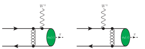
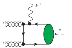
Figure 1: Leading-order contributions to the DVMP hard coefficient functions. The green blob stands for the pion wave function. Additional diagrams (not shown) may be obtained reversing directions of the quark lines and in case of the last diagram, also permuting vector boson vertices.

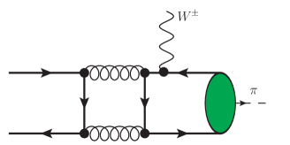
Figure 2: Sea quark contributions to the DVMP, which appear at next-to-leading-order. Additional diagrams (not shown) may be obtained reversing directions of the quark lines.

Straightforward evaluation of the diagrams shown in the Figures 1,2 yields for the coefficient function

$$\mathcal{C}_{\lambda\lambda^{\prime}}^{q} =\delta_{\lambda\lambda^{\prime}}\left(\eta_{-}^{q}c_{-}^{(q)}\left(x,\,\xi\right)+{\rm sgn}(\lambda)\eta_{+}^{q}c_{+}^{(q)}\left(x,\,\xi\right)+\mathcal{O}\left(\frac{m^{2}}{Q^{2}}\right)+\mathcal{O}\left(\alpha_{s}^{2}\left(\mu_{R}^{2}\right)\right)\right),$$ (27)

where the process-dependent flavor factors $\eta_{V\pm}^{q},\,\eta_{A\pm}^{q}$ are the same for $J^{P}=0^{-}$- and $1^{-}$mesons, and are given explicitly in Table 1 . Also, in (27) we introduced the shorthand notation

Table 1: The flavor coefficients $\eta_{\pm}^{q}$ for several meson production processes discussed in this paper. We use the notation $q=u,d,s,...$ $\{M^{\pm,0},M_{s}^{\pm,0}\}=\{\pi^{\pm,0},\,K^{\pm,0}\}$ mesons in $J^{P}=0^{-}$multiplet, and $\{M^{\pm,0},M_{s}^{\pm,0}\}=\{\rho^{\pm,0},\,K^{*\pm,0}\}$ mesons in $J^{P}=1^{-}$multiplet. As commented in the text, CC currents could be studied either in electron-induced processes (so $\{\ell,\ell^{\prime}\}=\{e,\,\nu_{e}\}$) or in neutrino-induced processes, $\{\ell,\,\ell^{\prime}\}=\{\bar{\nu}_{e},\,e^{+}\}$. For the case of CC mediated processes, the $V-A$ structure of the charged current implies $\eta_{V\pm}^{q}=\eta_{\pm}^{q},\quad\eta_{A\pm}^{q}=-\eta_{\pm}^{q}$.

Process	$\eta_{+}^{q}$	$\eta_{-}^{q}$		Process	$\eta_{+}^{q}$	$\eta_{-}^{q}$
$\ell\,p\to\ell^{\prime}\,M^{-}p$	$V_{ud}\delta_{qd}$	$V_{ud}\delta_{qu}$		$\ell\,p\to\ell^{\prime}M^{0}n$	$V_{ud}\frac{\delta_{qu}-\delta_{qd}}{\sqrt{2}}$	$-V_{ud}\frac{\delta_{qu}-\delta_{qd}}{\sqrt{2}}$
$\ell\,p\to\ell^{\prime}M^{0}n$	$V_{ud}\frac{\delta_{qu}-\delta_{qd}}{\sqrt{2}}$	$-V_{ud}\frac{\delta_{qu}-\delta_{qd}}{\sqrt{2}}$		$\ell\,p\to\ell^{\prime}M^{-}n$	$V_{ud}\delta_{qu}$	$V_{ud}\delta_{qd}$
$\ell\,p\to\ell^{\prime}M_{s}^{-}p$	$V_{us}\delta_{qs}$	$V_{us}\delta_{qs}$		$\ell\,n\to\ell^{\prime}M_{s}^{0}\Sigma^{-}$	0	$-V_{ud}\left(\delta_{qu}-\delta_{qs}\right)$

$$c_{\pm}^{(q)}\left(x,\xi\right) = \frac{8\pi i}{9}\frac{\alpha_{s}\left(\mu_{R}^{2}\right)f_{M}}{Q}\frac{1}{x\pm\xi\mp i0}\int_{0}^{1}dz\,\frac{\phi_{2}\left(z\right)}{z}\left(1+\frac{\alpha_{s}\left(\mu_{r}^{2}\right)}{2\pi}T^{(1)}\left(\frac{\xi\pm x}{2\xi},\,z\right)\right),$$ (28)

where $\phi_{2}(z)$ is the twist-2 meson distribution amplitude (DA). The function $T^{(1)}\left(v,\,z\right)$ in (28) encodes NLO corrections to the coefficient function and is given explicitly in the Appendix A. In general, we could expect that the spin structure of the coefficient function $\mathcal{C}_{\lambda}^{q}$ should depend on the quantum numbers of the produced mesons, however in the leading twist this is not so. This happens because at leading twist the distribution amplitudes of the $J^{P}=0^{-}$ and $1^{-}$ mesons differ only by an additional $\gamma_{5}$ in the corresponding quark operator and $V-A$ structure of charged current. From a trivial identity

$$\gamma_{\mu}\left(1-\gamma_{5}\right)\gamma_{\alpha_{1}}S\left(p_{1}\right)...\gamma_{\alpha_{n}}S\left(p_{n}\right)\gamma_{\pm}\gamma_{5}=\gamma_{\mu}\left(1-\gamma_{5}\right)\gamma_{\alpha_{1}}S\left(p_{1}\right)...\gamma_{\alpha_{n}}S\left(p_{n}\right)\gamma_{\pm}$$ (29)

where $S\left(p_{i}\right)$ are the quark propagators (massless in the Bjorken limit), we may conclude that for charged currents the amplitudes of $\rho$- and $\pi$-production coincide to any order in the strong coupling constant $\alpha_{s}\left(Q^{2}\right)$. The corrections due to finite mass of the quarks are $\sim\mathcal{O}(m_{q}/Q)$, and are numerically negligible for light quarks. In the twist-three case, similar arguments hold for the two-parton distribution amplitudes, yet for the contributions of the three-parton DAs this is no longer so. For this reason, we may use the above-mentioned substitutions (9,10,11) to relate the pion and $\rho$-meson distribution amplitudes.

In the leading order over $\alpha_{s}$, the ratio $R_{\rho/\pi}$ defined in (1) is constant and is given by the ratio of the minus-first moments $\left\langle\phi_{2,\,||,\rho}^{-1}\right\rangle$ and $\left\langle\phi_{2,\pi}^{-1}\right\rangle$. In terms of the conformal expansion coefficients $a_{2n}$ defined in (12), the moments may be evaluated exactly and are given by $\left\langle\phi_{2}^{-1}\right\rangle=1+\sum_{n}a_{2n}$, so the ratio (1) is given by

$$R_{\rho/\pi}\approx\left(f_{\rho}/f_{\pi}\right)^{2}\left(\frac{1+\sum a_{2n,\rho}^{(||)}}{1+\sum a_{2n,\pi}}\right)^{2}.$$ (30)

At this order all the expansion coefficients $r_{2n}$ defined in (15) are equal to unity, $r_{2n}\left(x_{B},\,Q^{2}\right)=1$, and do not depend on $\left(x_{B},\,Q^{2}\right)$. In the next-to-leading order there are $\delta r_{2n}\sim\mathcal{O}\left(\alpha_{s}\right)$ corrections, given explicitly in Appendix  A. The numerical values of the coefficients are discussed in detail in the following Section III.

II.3 Twist-three corrections

In the Bjorken limit, it is expected that the dominant contribution should come from the twist-two GPDs $H,\,E,\,\tilde{H},\,\tilde{E}$. However, as was shown in  Defurne:2016eiy , in moderate-energy experiments the typical values of virtuality $Q$ are only two or three times larger than the mass of the nucleon $m_{N}$. For this reason it is important to assess how large are the omitted higher-twist contributions.

Technically the evaluation of the twist-three contributions is quite challenging, because the are many different contributions, and for some of them (see e.g. three-parton contributions analyzed in Anikin:2009bf ; Anikin:2009hk ) numerical estimates are currently challenging due to lack of reliable phenomenological restrictions on multiparton distributions. In this paper we will restrict ourselves to the estimates of higher twist contributions due to two-parton twist-three components of the meson wave functions, which are expected to give the largest contribution to the difference between pion and $\rho$-meson cross-sections. The corresponding twist-three DAs for pion and $\rho$-meson were defined in Section II.1. Previously this analysis has been done by us in the context of neutrino-production Kopeliovich:2014pea and pion production by charged currents Siddikov:2017nku , and here we briefly repeat it for the case of charged current meson production. For the case of $\rho$-meson the amplitudes might be obtained from pion amplitude by the substitution (10, 11). The twist-three meson DAs probe the so-called transversity GPDs, which contribute to the amplitude (23) as

$$\delta\mathcal{H}_{\nu^{\prime}\lambda^{\prime},\nu\lambda}^{q} =\left(m_{\nu^{\prime}\nu}^{q}\delta_{\lambda,-}\delta_{\lambda^{\prime},+}+n_{\nu^{\prime}\nu}^{q}\delta_{\lambda,+}\delta_{\lambda^{\prime},-}\right),$$ (31)

where the coefficients $m_{\pm,\pm}^{q}$ and $n_{\pm,\pm}^{q}$ are linear combinations of the transversity GPDs,

$$m_{--}^{q} =\frac{\sqrt{-t^{\prime}}}{4m}\left[2\tilde{H}_{T}^{q}\,+(1+\xi)E_{T}^{q}-(1+\xi)\tilde{E}_{T}^{q}\right],$$ (32)

$$m_{-+}^{q} =\sqrt{1-\xi^{2}}\frac{t^{\prime}}{4m^{2}}\tilde{H}_{T}^{q},$$ (33)

$$m_{+-}^{q} =\sqrt{1-\xi^{2}}\left[H_{T}^{q}-\frac{\xi^{2}}{1-\xi^{2}}E_{T}^{q}+\frac{\xi}{1-\xi^{2}}\tilde{E}_{T}^{q}-\frac{t^{\prime}}{4m^{2}}\tilde{H}_{T}^{q}\right],$$ (34)

$$m_{++}^{q} =\frac{\sqrt{-t^{\prime}}}{4m}\left[2\tilde{H}_{T}^{q}+(1-\xi)E_{T}^{q}+(1-\xi)\tilde{E}_{T}^{q}\right],$$ (35)

$$n_{--}^{q} =-\frac{\sqrt{-t^{\prime}}}{4m}\left(2\tilde{H}_{T}^{q}+(1-\xi)E_{T}^{q}+(1-\xi)\tilde{E}_{T}^{q}\right),$$ (36)

$$n_{-+}^{q} =\sqrt{1-\xi^{2}}\left(H_{T}^{q}-\frac{\xi^{2}}{1-\xi^{2}}E_{T}^{q}+\frac{\xi}{1-\xi^{2}}\tilde{E}_{T}^{q}-\frac{t^{\prime}}{4m^{2}}\tilde{H}_{T}^{q}\right),$$ (37)

$$n_{+-}^{q} =\sqrt{1-\xi^{2}}\frac{t^{\prime}}{4m^{2}}\tilde{H}_{T}^{q},$$ (38)

$$n_{++}^{q} =-\frac{\sqrt{-t^{\prime}}}{4m}\left(2\tilde{H}_{T}^{q}+(1+\xi)E_{T}^{q}-(1+\xi)\tilde{E}_{T}^{q}\right),$$ (39)

and we introduced a shorthand notation $t^{\prime}=-\Delta_{\perp}^{2}/(1-\xi^{2})$; $\Delta_{\perp}=p_{2,\perp}-p_{1,\perp}$ is the transverse part of the momentum transfer. The coefficient function (27) also gets an additional nondiagonal in parton helicity contribution,

$$\delta\mathcal{C}_{\lambda^{\prime}0,\lambda\mu}^{q} ==\delta_{\mu,+}\delta_{\lambda,-}\delta_{\lambda^{\prime},+}\left(S_{A}^{q}-S_{V}^{q}\right)+\delta_{\mu,-}\delta_{\lambda,+}\delta_{\lambda^{\prime},-}\left(S_{A}^{q}+S_{V}^{q}\right)+\mathcal{O}\left(\frac{m^{2}}{Q^{2}}\right),$$ (40)

where we introduced the shorthand notations

$$S_{A}^{q} = \int dz\,\left(\left(\eta_{A+}^{q}c_{+}^{(3,p)}\left(x,\xi\right)-\eta_{A-}^{q}c_{-}^{(3,p)}\left(x,\xi\right)\right)+2\left(\eta_{A-}^{q}c_{-}^{(3,\sigma)}\left(x,\xi\right)+\eta_{A+}^{q}c_{+}^{(3,\sigma)}\left(x,\xi\right)\right)\right),$$ (41)

$$S_{V}^{q} = \int dz\,\left(\left(\eta_{V+}^{q}c_{+}^{(3,p)}\left(x,\xi\right)+\eta_{V-}^{q}c_{-}^{(3,p)}\left(x,\xi\right)\right)+2\left(\eta_{V+}^{q}c_{+}^{(3,\sigma)}\left(x,\xi\right)-\eta_{V-}^{q}c_{-}^{(3,\sigma)}\left(x,\xi\right)\right)\right),$$ (42)

$$c_{+}^{(3,i)}\left(x,\xi\right)=\frac{4\pi i\alpha_{s}f_{\pi}\xi}{9\,Q^{2}}\int_{0}^{1}dz\frac{\phi_{3,i}(z)}{z\,(x+\xi)^{2}},\quad c_{-}^{(3,i)}\left(x,\xi\right)=\frac{4\pi i\alpha_{s}f_{\pi}\xi}{9\,Q^{2}}\int_{0}^{1}dz\frac{\phi_{3,i}(z)}{(1-z)(x-\xi)^{2}};$$ (43)

and the twist-three pion distributions are defined in Section II.1. Due to symmetry of $\phi_{p}$ and antisymmetry of $\phi_{\sigma}$ with respect to charge conjugation, the dependence on the pion DAs factorizes in the collinear approximation and contributes only as the minus first moment of the linear combination of the twist-3 DAs, $\phi_{3}^{(p)}(z)+2\phi_{3}^{(\sigma)}(z)$,

$$\left\langle\phi_{3}^{-1}\right\rangle=\int_{0}^{1}dz\frac{\phi_{3}^{(p)}\left(z\right)+2\phi_{3}^{(\sigma)}\left(z\right)}{z}.$$ (44)

In general case the coefficient function  (43) leads to collinear divergencies near the points $x=\pm\xi$, when substituted to (20). As was noted in Goloskokov:2009ia , this singularity is naturally regularized by the small transverse momentum of the quarks inside the meson. Such regularization modifies (43) to

$$c_{+}^{(3,i)}\left(x,\xi\right) =\frac{4\pi i\alpha_{s}f_{\pi}\xi}{9\,Q^{2}}\int_{0}^{1}dz\,d^{2}l_{\perp}\frac{\phi_{3,i}\left(z,\,l_{\perp}\right)}{(x+\xi-i0)\left(z(x+\xi)+\frac{2\xi\,l_{\perp}^{2}}{Q^{2}}\right)},$$ (45)

$$c_{-}^{(3,i)}\left(x,\xi\right) =\frac{4\pi i\alpha_{s}f_{\pi}\xi}{9\,Q^{2}}\int_{0}^{1}dz\,d^{2}l_{\perp}\frac{\phi_{3,i}\left(z,\,l_{\perp}\right)}{(x-\xi+i0)\left((1-z)(x-\xi)-\frac{2\xi\,l_{\perp}^{2}}{Q^{2}}\right)},$$ (46)

where $l_{\perp}$ is the transverse momentum of the quark, and we tacitly assume absence of any other transverse momenta in the coefficient function. Due to interference of the leading twist and twist-three contributions, the total cross-section acquires dependence on the angle $\varphi$ between lepton scattering and pion production planes,

$$\frac{d\sigma}{dt\,dx_{B}dQ^{2}d\varphi} =\epsilon\frac{d\sigma_{L}}{dt\,dx_{B}dQ^{2}d\varphi}+\frac{d\sigma_{T}}{dt\,dx_{B}dQ^{2}d\varphi}+\sqrt{\epsilon(1+\epsilon)}\cos\varphi\frac{d\sigma_{LT}}{dt\,dx_{B}dQ^{2}d\varphi}$$ (47)

$$+\epsilon\cos\left(2\varphi\right)\frac{d\sigma_{TT}}{dt\,dx_{B}dQ^{2}d\varphi}+\sqrt{\epsilon(1+\epsilon)}\sin\varphi\frac{d\sigma_{L^{\prime}T}}{dt\,dx_{B}dQ^{2}d\varphi}+\epsilon\sin\left(2\varphi\right)\frac{d\sigma_{T^{\prime}T}}{dt\,dx_{B}dQ^{2}d\varphi},$$

where we introduced the shorthand notations

$$\epsilon=\frac{1-y-\frac{\gamma^{2}y^{2}}{4}}{1-y+\frac{y^{2}}{2}+\frac{\gamma^{2}y^{2}}{4}}.$$ (48)

$$\frac{d\sigma_{L}}{dt\,dx_{B}dQ^{2}d\varphi} =\frac{\Gamma\,\sigma_{00}}{2\pi\epsilon}$$ (49)

$$\frac{d\sigma_{T}}{dt\,dx_{B}dQ^{2}d\varphi} =\frac{\Gamma}{2\pi\epsilon}\,\left(\frac{\sigma_{++}+\sigma_{--}}{2}+\frac{1}{2}\sqrt{1-\epsilon^{2}}\frac{\sigma_{++}-\sigma_{--}}{2}\right)$$ (50)

$$\frac{d\sigma_{LT}}{dt\,dx_{B}dQ^{2}d\varphi} =\frac{\Gamma}{2\pi\epsilon}\,\left({\rm Re}\left(\sigma_{0+}-\sigma_{0-}\right)+\frac{1}{2}\sqrt{\frac{1-\epsilon}{1+\epsilon}}{\rm Re}\left(\sigma_{0+}+\sigma_{0-}\right)\right)$$ (51)

$$\frac{d\sigma_{TT}}{dt\,dx_{B}dQ^{2}d\varphi} =-\frac{\Gamma}{2\pi\epsilon}\,{\rm Re}\left(\sigma_{+-}\right)$$ (52)

$$\frac{d\sigma_{L^{\prime}T}}{dt\,dx_{B}dQ^{2}d\varphi} =-\frac{\Gamma}{2\pi\epsilon}\,\left({\rm Im}\left(\sigma_{+0}+\sigma_{-0}\right)-\frac{1}{2}\sqrt{\frac{1-\epsilon}{1+\epsilon}}{\rm Im}\left(\sigma_{-0}-\sigma_{+0}\right)\right)$$ (53)

$$\frac{d\sigma_{T^{\prime}T}}{dt\,dx_{B}dQ^{2}d\varphi} =-\frac{\Gamma}{2\pi\epsilon}\,{\rm Im}\left(\sigma_{+-}\right)$$ (54)

and the subindices $\alpha,\beta$ in

$$\sigma_{\alpha\beta}=\sum_{\nu\nu^{\prime}}\mathcal{A}_{\nu^{\prime}0,\nu\alpha}^{*}\mathcal{A}_{\nu^{\prime}0,\nu\beta},$$ (55)

refer to the polarizations of intermediate heavy boson in the amplitude and its conjugate. As we will see below, in JLAB kinematics the contribution of higher twist corrections is small, and for this reason we will quantify their size in terms of the angular harmonics $c_{n},\,s_{n}$, normalizing the total cross-section to the cross-section of the dominant DVMP process defined as Siddikov:2017nku

$$\frac{d^{4}\sigma^{(tot)}}{dt\,d\ln x_{Bj}\,dQ^{2}d\varphi}=\frac{1}{2\pi}\frac{d^{4}\sigma^{(DVMP)}}{dt\,d\ln x_{Bj}\,dQ^{2}}\left(1+\sum_{n=0}^{2}c_{n}\cos(n\varphi)+s_{1}\sin(\varphi)\right).$$ (56)

The main purpose of this study is to analyze the sensitivity of the ratio (1) to changes of the coefficients $r_{2n}$. For this reason in what follows we will focus on the evaluation of the harmonics $c_{0}$ and the corresponding cross-sections $d\sigma_{L}$ and $d\sigma_{T}$. The higher twist corrections contribute additively to the cross-section (no interference due to different spin structure), and as we will see below, in the kinematics of interest the cross-section $d\sigma_{T}\ll d\sigma_{L}$. For this reason the correction to the ratio (1) is small and is given by

$$\delta R^{{\rm twist}-3} \approx\underbrace{\frac{f_{\rho}^{2}}{f_{\pi}^{2}}\left(\frac{d\sigma_{T}^{(\rho)}}{\epsilon d\sigma_{L}^{(\rho)}}-\frac{d\sigma_{T}^{(\pi)}}{\epsilon d\sigma_{L}^{(\pi)}}\right)}_{\sim\mathcal{O}(1/Q)}+\mathcal{O}\left(\frac{1}{Q^{2}}\right)=\frac{f_{\rho}^{2}}{f_{\pi}^{2}}\left(c_{0,\rho}-c_{0,\pi}\right)+\mathcal{O}\left(\frac{1}{Q^{2}}\right):=\frac{f_{\rho}^{2}}{f_{\pi}^{2}}\Delta c_{0},$$ (57)

$$\Delta c_{0} =c_{0,\rho}-c_{0,\pi},$$ (58)

where $c_{0,\rho}$ and $c_{0,\pi}$ are the zeroth order harmonics (angular-independent contributions of twist-3 terms) of the $\rho$-meson and pion respectively. At present, the values of the twist-three $\rho$-meson DAs are poorly known (especially for the case of $\rho$-mesons), and for this reason we will assume that it changes from 0 up to the same value as for pion, (16).

III Results and discussion

In this section we would like to present numerical results for the charged current pion production. For the sake of definiteness, for numerical estimates we use the Kroll-Goloskokov parameterization of GPDs Goloskokov:2006hr ; Goloskokov:2007nt ; Goloskokov:2008ib ; Goloskokov:2009ia ; Goloskokov:2011rd . For illustration, we will start the discussion assuming dominance of the twist two corrections, and neglecting the deviations from the asymptotic form encoded in the coefficients $a_{2n}$ in (12). In this case the difference between pion and $\rho$-meson cross-sections becomes negligible (we may neglect the so-called “kinematic” higher twist effects $\sim\mathcal{O}\left(M_{\pi,\rho}^{2}/Q^{2}\right)$ in the Bjorken limit).

In the left panel of the Figure 3 we show predictions for the differential cross-section $d\sigma/dx_{B}\,dQ^{2}$ for charged meson ($\rho^{-},\,\pi^{-}$) production, within JLab kinematics. We expect that for typical instant luminosities $\sim 10^{35}{\rm cm^{-2}s^{-1}}$, easonable statistics could be collected after 30-60 days of running. At fixed electron energy $E_{e}=11\,{\rm GeV}$ and virtuality $Q^{2}$, the cross-section as function of $x_{B}$ has a typical bump-like shape, which is explained by an interplay of two factors. For small $x_{B}\sim Q^{2}/2m_{N}E_{e}$ the elasticity $y$ defined in (19) approaches one, which causes a suppression due to a prefactor $\Gamma$ in (17). In the opposite limit, the suppression $\sim(1-x)^{n}$ is due to the implemented parameterization of GPDs. In the evaluation of the coefficient function we take into account NLO corrections, which give a sizable contribution for $Q^{2}\lesssim 10\,{\rm GeV}^{2}$. The band around the curves reflects the uncertainty of the predictions due to higher order corrections, which was obtained varying the factorization scale $\mu_{F}$ in the range $\mu_{F}\in\left(Q/2,\,2Q\right)$ (see Diehl:2003ny ; Goloskokov:2009ia ; Goloskokov:2011rd ; Diehl:2007hd ; Pire:2017lfj for more details). The amplitudes in this region get the dominant contribution from the GPDs $H^{u},\,H^{d}$, whereas helicity flip and gluon GPDs give a minor ($\sim$10%) correction to the full cross-section. In the right panel we show the cross-section for the kinematics of EIC experiment, assuming a center-of-mass energy $\sqrt{s_{ep}}\approx 100\,{\rm GeV}.$ At present the exact energy $\sqrt{s_{ep}}$, which will be available at EIC, is not known, yet reevaluation for other energies $\sqrt{s}_{ep}$ is quite straightforward and might be obtained by rescaling the $y$-dependent prefactor (18). The effects of this factor are pronounced at small $x_{B}\ll 1$, where it leads to a suppression of the cross-section.

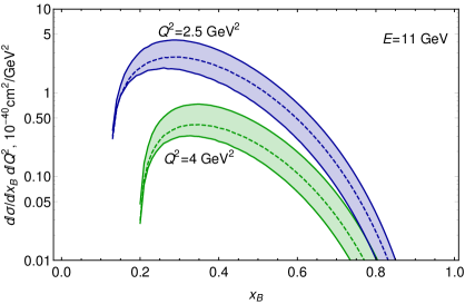
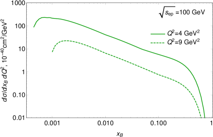
Figure 3: (color online) Left plot: Charged current meson production cross-section on a proton target, within JLab kinematics (fixed electron energy $E=11\,{\rm GeV}$). Evaluations are performed using NLO coefficient functions, as discussed in Section II.2. The width of the band represents the uncertainty due to the factorization scale choice $\mu_{F}\in\left(Q/2,\,2Q\right)$, as explained in the text. Right plot: $x_{B}$-dependence of the cross-section in EIC kinematics with $\sqrt{s}_{ep}\approx 100\,{\rm GeV}$. For other values of $\sqrt{s}_{ep}$ and fixed $\left(x_{B},\,Q^{2}\right)$ the cross-section might be obtained by rescaling the factor (18). This factor is responsible for the suppression of the cross-section at small $x_{B}\ll 1$ and at fixed energy $\sqrt{s_{ep}}$.

In order to quantize the sensitivity of the cross-section to deviation of the meson DA from its asymptotic form, in Figure 4 we show the dependence of the first two coefficients $r_{2}\left(x_{B},\,Q^{2}\right)$ and $r_{4}\left(x_{B},\,Q^{2}\right)$, defined in (1), as functions of $x_{B}$ and $Q^{2}$. These coefficients do not depend on the energy of the electron beam $E$, because at fixed $\left(x_{B},\,Q^{2}\right)$ the dependence on $E$ contributes only via a common $y$-dependent prefactor in (18), which does not contribute to $r_{2n}$. The dependence of $r_{2n}$ on $Q^{2}$ is very mild and is due to the logarithmic dependence of running coupling in the NLO contribution. The dependence of $r_{2n}$ on $x_{B}$ exists due to the different $x_{B}$-dependence of the leading order and next-to-lading order amplitudes. The fact that the evaluated ratios $r_{2n}$ have a very mild dependence on $Q^{2}$ and on $x_{B}$ (for $x_{B}\lesssim 0.3$) implies that the ratio of the cross-sections (1) only mildly depends on $(x_{B},\,Q^{2})$, and its value is almost entirely determined by the values of parameters

$$a_{2}=a_{2}^{(\rho)}-a_{2}^{(\pi)},\qquad a_{4}=a_{4}^{(\rho)}-a_{4}^{(\pi)}.$$ (59)

As can be seen from the Figure 4, for the currently expected phenomenological values of parameters $a_{2},a_{4}$ in the range (13), the ratio (1) changes up to 20%. Since the expected values of $a_{2},\,a_{4}$ are quite small, we may neglect the contributions of quadratic terms, so we expect that $R_{\rho/\pi}$ is mostly sensitive to the combination

$$\left(a_{2}+\frac{r_{4}\left(x_{B},\,Q^{2}\right)}{r_{2}\left(x_{B},\,Q^{2}\right)}a_{4}\right).$$ (60)

Given that the functions $r_{2}\left(x,\,Q^{2}\right)$, $r_{4}\left(x,\,Q^{2}\right)$ are known, measurement of $R_{\rho/\pi}$ in a sufficiently large kinematical range could allow us to extract separately the values of $a_{2}$ and $a_{4}$.

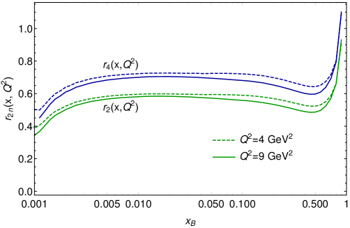
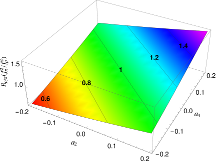
Figure 4: (color online) Left: Values of the coefficients $r_{2n}\left(x_{B},\,Q^{2}\right).$ The two bottom curves correspond to $r_{2}\left(x_{B},\,Q^{2}\right);$ the two upper curves correspond to $r_{4}\left(x_{B},\,Q^{2}\right).$ For both cases dashed lines correspond to $Q^{2}=4\,{\rm GeV}^{2}$, solid lines correspond to $Q^{2}=9\,{\rm GeV}^{2}.$ All evaluations performed with account of NLO correction. See the text for more explanations of the behaviour of the curves. Right: expected value of the variable $R_{\rho/\pi}\left(f_{\pi}/f_{\rho}\right)^{2}$ as a function of possible values of $a_{2}^{(\rho-\pi)}$ and $a_{4}^{(\rho-\pi)}$ for $x_{B}=0.1$ and $Q^{2}=4\,{\rm GeV}^{2}$. For the case of asymptotic form distributions of both mesons ($a_{2}^{(\rho-\pi)}=a_{4}^{(\rho-\pi)}=0$) the variable $R_{\rho/\pi}\left(f_{\pi}/f_{\rho}\right)^{2}=1$.

As we explained in the previous section, for the case of the twist-three harmonics, we are only interested in the contribution of the term $c_{0}$ in (56), which is the only term contributing to the $\varphi$-integrated cross-sections. From Figure 5, we can see that the contribution of this term in the region of interest is negligible and does not exceed a few per cent. Its relative contribution increases in the region $x_{B}\gtrsim 0.6-0.7$ and it might reach up to 10 per cent. However, the cross-section is strongly suppressed in that region, and the experimental statistics is quite poor, so for this reason we expect that this region will not give a strong constraint on the constructed parameterizations of the GPDs. In the region $x_{B}\approx 0.1-0.3$, which gives the dominant contribution within JLab kinematics, we expect that the effects of the higher twist corrections will give just a couple of per cent correction, and will not affect significantly the ratio $R\left(a_{2},\,a_{4}\right)$, shown in the right panel of Figure 4. The effect of higher twist corrections decreases as a function of $Q$ and becomes almost negligible for $Q^{2}\gtrsim 10\,{\rm GeV}^{2}.$

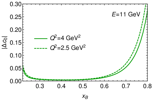
Figure 5: (color online) Upper values of the coefficient $\left|\Delta c_{0}\right|$ for several values of $Q^{2}$, within JLab kinematics ($E=11$ GeV).

For deeply virtual meson production in other channels (e.g. production of kaons and $K^{*}$-mesons) the cross-sections have a similar shape, although their values are smaller. Besides, the amplitudes of these processes get comparable contributions from GPDs of different partons, and for this reason the restrictions imposed by experimental data on GPDs of individual partons are less binding (see Siddikov:2017nku for more details). Moreover, experimentally these channels present more challenges and therefore will not be considered here. The contribution of the higher twist corrections might be estimated similarly in terms of higher twist harmonics.

IV Conclusions

In this paper we studied the contributions for $\rho$-meson production in Bjorken kinematics. We found that the production of both parity conjugate mesons ($\rho$ and $\pi$) in charged current processes allows for a very clean probe of the generalized parton distributions, and the ratio (1) provides the possibility of clearly distinguishing contributions of higher twist corrections. More precisely, since the cross-sections of both processes are sensitive to the same set of GPDs, the ratio (1) should be almost constant in the case of the leading twist dominance, and the value of this constant depends only on the DAs of the produced mesons. The presence of large higher twist corrections would reveal itself via a pronounced dependence of the ratio (1) on both $x_{B}$ and $Q^{2}$. We expect that such processes might be studied either in JLab future neutrino-induced experiments or in electron-induced experiments in JLab and EIC. We estimated the cross-sections in the kinematics of upgraded 12 GeV Jefferson Laboratory experiments, as well as in the kinematics of the future Electron Ion Collider, and found that the process can be measured with reasonable statistics. A code for the evaluation of the cross-sections with various GPD models is available on demand.

Appendix A NLO coefficient function

The function $T^{(1)}\left(v,\,z\right)$ in (65) encodes NLO corrections to the coefficient function. Explicitly, this function is given by

$$T^{(1)}\left(v,\,z\right) =\frac{1}{2vz}\left[\frac{4}{3}\left([3+\ln(v\,z)]\,\ln\left(\frac{Q^{2}}{\mu_{F}^{2}}\right)+\frac{1}{2}\ln^{2}\left(v\,z\right)+3\ln(v\,z)-\frac{\ln\bar{v}}{2\bar{v}}-\frac{\ln\bar{z}}{2\bar{z}}-\frac{14}{3}\right)\right.$$ (61)

$$+\beta_{0}\left(\frac{5}{3}-\ln(v\,z)-\ln\left(\frac{Q^{2}}{\mu_{R}^{2}}\right)\right)$$

$$-\frac{1}{6}\left(2\frac{\bar{v}\,v^{2}+\bar{z}\,z^{2}}{(v-z)^{3}}\left[{\rm Li}_{2}(\bar{z})-{\rm Li}_{2}(\bar{v})+{\rm Li}_{2}(v)-{\rm Li}_{2}(z)+\ln\bar{v}\,\ln z-\ln\bar{z}\,\ln v\right]\right.$$

$$+2\frac{v+z-2v\,z}{(v-z)^{2}}\ln\left(\bar{v}\bar{z}\right)+2\left[{\rm Li}_{2}(\bar{z})+{\rm Li}_{2}(\bar{v})-{\rm Li}_{2}(z)-{\rm Li}_{2}(v)+\ln\bar{v}\,\ln z+\ln\bar{z}\,\ln v\right]$$

$$+\left.\left.4\frac{v\,z\,\ln(v\,z)}{(v-z)^{2}}-4\ln\bar{v}\,\ln\bar{z}-\frac{20}{3}\right)\right],$$

where $\beta_{0}=\frac{11}{3}N_{c}-\frac{2}{3}N_{f}$, ${\rm Li}_{2}(z)$ is the dilogarithm function, and $\mu_{R}$ and $\mu_{F}$ are the renormalization and factorization scales respectively. For the vector meson production in processes when the internal state of the hadron is not changed, the additional contribution comes from gluons and singlet (sea) quarks Belitsky:2001nq ; Ivanov:2004zv ; Diehl:2007hd  ,

$$c^{(g)}\left(x,\xi\right) = \left(\int dz\frac{\phi_{2,\pi}\left(z\right)}{z\,(1-z)}\right)\frac{2\pi i}{3}\frac{\alpha_{s}\left(\mu_{R}^{2}\right)f_{M}}{Q}\frac{\xi}{\left(\xi+x-i0\right)\left(\xi-x-i0\right)}\left(1+\frac{\alpha_{s}\left(\mu_{r}^{2}\right)}{4\pi}\mathcal{I}^{(g)}\left(\frac{\xi-x}{2\xi},\,z\right)\right),$$ (62)

$$\mathcal{I}^{(g)}\left(v,\,z\right) = \left(\ln\left(\frac{Q^{2}}{\mu_{F}^{2}}\right)-1\right)\left[\frac{\beta_{0}}{2}+C_{A}\left[\left(1-v\right)^{2}+v^{2}\right]\left(\frac{\ln\left(1-v\right)}{v}+\frac{\ln v}{1-v}\right)-\frac{C_{F}}{2}\left(\frac{v\ln v}{1-v}+\frac{\left(1-v\right)\ln\left(1-v\right)}{v}\right)\right.$$

$$+\left.C_{F}\left(\frac{3}{2}+2\,z\ln\left(1-z\right)\right)\right]-2\,C_{F}-\frac{\beta_{0}}{2}\left(\ln\left(\frac{Q^{2}}{\mu_{R}^{2}}\right)-1\right)-\frac{C_{F}\left(1-2\,v\right)}{2\,\left(z-v\right)}R\left(z,\,v\right)$$

$$+\frac{\left(2C_{A}-C_{F}\right)}{4}\left(\frac{v\,\ln^{2}v}{1-v}+\frac{\left(1-v\right)\ln^{2}\left(1-v\right)}{v}\right)+C_{F}(1+3\,z)\ln\left(1-z\right)+$$

$$+\left(\ln\,v+\ln\left(1-v\right)\right)\left[C_{F}\left(1-z\right)\ln\,z-\frac{1}{4}+2C_{F}-C_{A}\right]$$

$$+\frac{C_{A}}{2}\left(\ln\left(z\,(1-z)\right)-2\right)\left[\frac{v\,\ln v}{1-v}+\frac{\left(1-v\right)\,\ln\left(1-v\right)}{v}\right]$$

$$+C_{F}z\,\ln^{2}\left(1-z\right)+\frac{C_{A}}{2}\left(1-2\,v\right)\ln\left(\frac{v}{1-v}\right)\left[\frac{3}{2}+\ln\left(z\,\left(1-z\right)\right)+\ln\left(v\,\left(1-v\right)\right)\right]$$

$$+\left(C_{F}\left((z-v)^{2}-v\,(1-v)\right)-\left(C_{F}-\frac{C_{A}}{2}\right)(z-v)(1-2v)\right)\times$$

$$\times\left[-\frac{R(z,v)}{(z-v)^{2}}+\frac{\ln v+\ln z-\ln\left(1-v\right)-\ln\left(1-z\right)}{2\left(z-v\right)}+\frac{(z-v)^{2}-v(1-v)}{(z-v)^{3}}H(z,v)\right]$$

$$+\left\{\frac{}{}z\to 1-z\right\},$$

$$C_{F} = \frac{N_{c}^{2}-1}{2N_{c}},\quad C_{A}=N_{c}.$$ (64)

$$c_{\pm}^{(s)}\left(x,\xi\right) = -\left(\int dz\frac{\phi_{2,\pi}\left(z\right)}{z\,(1-z)}\right)\frac{4i\alpha_{s}^{2}\left(\mu_{R}^{2}\right)f_{M}}{9\,Q}\mathcal{I}^{(s)}\left(\frac{x\pm\xi}{2\xi},\,z\right),$$ (65)

$$\mathcal{I}^{(s)}\left(v,\,z\right) = \left(1-2\,v\right)\left(\frac{\ln v}{1-v}+\frac{\ln(1-v)}{v}\right)\ln\left(\frac{Q^{2}z}{\mu_{F}^{2}}\right)+\frac{1-2v}{2}\left[\frac{\ln^{2}v}{1-v}+\frac{\ln^{2}\left(1-v\right)}{v}\right]$$

$$-\frac{R(v,\,z)}{z-v}-\frac{\left(1-v\right)\ln\left(1-v\right)-v\ln v}{v\left(1-v\right)}+\frac{\left(z-v\right)^{2}-v\left(1-v\right)}{\left(z-v\right)^{2}}H\left(v,z\right)+\left\{\frac{}{}z\to 1-z\right\},$$

$$R\left(v,\,z\right) = z\ln v+(1-z)\,\ln\left(1-v\right)+z\,\ln z+\left(1-v\right)\ln\left(1-v\right),$$ (67)

$$H\left(v,\,z\right) = {\rm Li}_{2}\left(1-v\right)-{\rm Li}_{2}\left(v\right)+{\rm Li}_{2}\left(z\right)-{\rm Li}_{2}\left(1-z\right)+\ln v\,\ln\left(1-z\right)-\ln\left(1-v\right)\ln\,z.$$ (68)

Some coefficient functions have non-analytic behavior $\sim\ln^{2}v$ for small $v\approx 0$ ($x=\pm\xi\mp i0$), which signals that the collinear approximation might be not valid near this point. This singularity in the collinear limit occurs due to the omission of the small transverse momentum $l_{M,\perp}$ of the quark inside a meson Goloskokov:2009ia . For this reason the contribution of the region $|v|\sim l_{M,\perp}^{2}/Q^{2}$ for finite $Q^{2}$ (below the Bjorken limit) should be treated with due care. However, a full evaluation of $T^{(1)}\left(v,\,z\right)$ beyond the collinear approximation (taking into account all higher twist corrections) presents a challenging problem and has not been done so far. It was observed in Diehl:2007hd , that the singular terms might be eliminated by a redefinition of the renormalization scale $\mu_{R}$, however near the point $v\approx 0$ the scale $\mu_{R}^{2}$ becomes soft, $\mu_{R}^{2}\sim z\,v\,Q^{2}\lesssim l_{\perp}^{2}$ which is another manifestation that nonperturbative effects become relevant. For this reason, sufficiently large value of $Q^{2}$ should be used to mitigate contributions of higher twist effects. As we will see below, for $Q^{2}\approx 4$ GeV² the contribution of this soft region is small, so the collinear factorization is reliable.

As was discussed in Section (II.1), the distribution amplitudes might be represented as (12), with major contribution from the terms with $n=0,\,1$ and $2.$ The corresponding expressions for the parton amplitudes (28,62,65) take a form Diehl:2007hd

$$c_{\pm,n}^{(q)}\left(x,\xi\right) = \frac{8\pi i}{9}\frac{\alpha_{s}\left(\mu_{R}^{2}\right)f_{M}}{Q}\frac{3}{x\pm\xi\mp i0}\left(1+\frac{\alpha_{s}\left(\mu_{r}^{2}\right)}{4\pi}t_{a,\,n}\left(\frac{\xi\pm x}{2\xi}\right)\right),$$ (69)

$$t_{a,0}(y) =\beta_{0}\left[\frac{19}{6}-\ln y-\ln\left(\frac{Q^{2}}{\mu_{R}^{2}}\right)\right]+C_{F}\biggl{[}\left(3+2\ln y\right)\,\ln\left(\frac{Q^{2}}{\mu_{GPD}^{2}}\right)-\frac{77}{6}-\left(\frac{1}{\bar{y}}-3\right)\ln y+\ln^{2}y\biggr{]}$$

$$\quad+\left(2C_{F}-C_{A}\right)\biggl{\{}-\frac{1}{3}-4(2-3y)\ln\bar{y}+2(1-6y)\ln y+4(1-3y)\,\bigl{(}{\rm Li}_{2}y-{\rm Li}_{2}\bar{y}\bigr{)}$$

$$\qquad\qquad+2(1-6y\bar{y})\left[3\bigl{(}{\rm Li}_{3}\bar{y}+{\rm Li}_{3}y\bigr{)}-\ln y\,{\rm Li}_{2}y-\ln\bar{y}\,{\rm Li}_{2}\bar{y}-\frac{\pi^{2}}{6}\,\bigl{(}\ln y+\ln\bar{y}\bigr{)}\right]\biggr{\}}\,.$$ (70)

$$t_{a,2}(y) =\beta_{0}\left[\frac{21}{4}-\ln y-\ln\frac{Q^{2}}{\mu_{R}^{2}}\right]+C_{F}\biggl{[}\left(3+2\ln y\right)\,\ln\frac{Q^{2}}{\mu_{GPD}^{2}}-\frac{25}{6}\,\ln\frac{Q^{2}}{\mu_{DA}^{2}}-\frac{1019}{72}-\left(\frac{1}{\bar{y}}+\frac{7}{6}\right)\ln y+\ln^{2}y\biggr{]}$$

$$\quad+\left(2C_{F}-C_{A}\right)\biggl{\{}\frac{401}{12}-255y+270y^{2}-\left(\frac{299}{3}-867y+1830y^{2}-1080y^{3}\right)\ln\bar{y}$$

$$\qquad+\left(\frac{56}{3}-357y+1290y^{2}-1080y^{3}\right)\ln y+2\,\bigl{(}22-291y+780y^{2}-540y^{3}\bigr{)}\,\bigl{(}{\rm Li}_{2}y-{\rm Li}_{2}\bar{y}\bigr{)}$$

$$\qquad+12\,\left(1-21y+106y^{2}-175y^{3}+90y^{4}\right)$$

$$\qquad\quad\times\biggl{[}3\bigl{(}{\rm Li}_{3}\bar{y}+{\rm Li}_{3}y\bigr{)}-\ln y\,{\rm Li}_{2}y-\ln\bar{y}\,{\rm Li}_{2}\bar{y}-\frac{\pi^{2}}{6}\,\bigl{(}\ln y+\ln\bar{y}\bigr{)}\biggr{]}\biggr{\}}\,,$$

$$t_{a,4}(y) =\beta_{0}\left[\frac{31}{5}-\ln y-\ln\frac{Q^{2}}{\mu_{R}^{2}}\right]$$

$$\quad+C_{F}\biggl{[}\left(3+2\ln y\right)\,\ln\frac{Q^{2}}{\mu_{GPD}^{2}}-\frac{91}{15}\,\ln\frac{Q^{2}}{\mu_{DA}^{2}}-\frac{10213}{900}-\left(\frac{1}{\bar{y}}+\frac{46}{15}\right)\ln y+\ln^{2}y\biggr{]}$$

$$\quad+\left(2C_{F}-C_{A}\right)\biggl{\{}\frac{4903}{40}-\frac{5775}{2}y+\frac{57085}{4}y^{2}-23310y^{3}+11970y^{4}$$

$$\qquad-\left(\frac{21109}{60}-\frac{41451}{5}y+\frac{103285}{2}y^{2}-125020y^{3}+129150y^{4}-47880y^{5}\right)\ln\bar{y}$$

$$\qquad+\left(\frac{2899}{60}-\frac{11001}{5}y+\frac{45535}{2}y^{2}-78400y^{3}+105210y^{4}-47880y^{5}\right)\ln y$$

$$\qquad+\bigl{(}137-4506y+35280y^{2}-100380y^{3}+117180y^{4}-47880y^{5}\bigr{)}\,\bigl{(}{\rm Li}_{2}y-{\rm Li}_{2}\bar{y}\bigr{)}\phantom{\biggl{[}\biggr{]}}$$

$$\qquad+30\,\bigl{(}1-48y+580y^{2}-2590y^{3}+5166y^{4}-4704y^{5}+1596y^{6}\bigr{)}\phantom{\biggl{[}\biggr{]}}$$

$$\qquad\quad\times\biggl{[}3\bigl{(}{\rm Li}_{3}\bar{y}+{\rm Li}_{3}y\bigr{)}-\ln y\,{\rm Li}_{2}y-\ln\bar{y}\,{\rm Li}_{2}\bar{y}-\frac{\pi^{2}}{6}\,\bigl{(}\ln y+\ln\bar{y}\bigr{)}\biggr{]}\biggr{\}}\,.$$ (71)

$$c_{n}^{(g)}\left(x,\xi\right) = \frac{2\pi i\alpha_{s}\left(\mu_{R}^{2}\right)f_{M}}{Q}\frac{\xi}{\left(\xi+x-i0\right)\left(\xi-x-i0\right)}\left(1+\frac{\alpha_{s}\left(\mu_{r}^{2}\right)}{4\pi}t_{g,\,n}\left(\frac{\xi-x}{2\xi}\right)\right),$$ (72)

where

$$t_{g,0}(y) =\biggl{[}2C_{A}\,(y^{2}+\bar{y}^{2})-C_{F}\,y\biggr{]}\frac{\ln y}{\bar{y}}\,\ln\frac{Q^{2}}{\mu_{GPD}^{2}}+\frac{\beta_{0}}{2}\,\ln\frac{\mu_{R}^{2}}{\mu_{GPD}^{2}}$$

$$\quad+C_{F}\biggl{[}-\frac{5}{2}+\left(\frac{1}{\bar{y}}+1-4y\right)\ln y-\frac{y}{2}\,\frac{\ln^{2}y}{\bar{y}}$$

$$\qquad\qquad-2(\bar{y}-y){\rm Li}_{2}\bar{y}-4y\bar{y}\biggl{(}3{\rm Li}_{3}\bar{y}-\ln y\,{\rm Li}_{2}y-\frac{\pi^{2}}{6}\ln y\biggr{)}\biggr{]}$$

$$\quad+C_{A}\left[-\left(\frac{6}{\bar{y}}-8y\right)\ln y+\left(\frac{1}{\bar{y}}-2y\right)\ln^{2}y+2(\bar{y}-y){\rm Li}_{2}\bar{y}\right]+\{y\to\bar{y}\}\,,$$

$$t_{g,2}(y) =\biggl{[}2C_{A}\,(y^{2}+\bar{y}^{2})-C_{F}\,y\biggr{]}\frac{\ln y}{\bar{y}}\,\ln\frac{Q^{2}}{\mu_{GPD}^{2}}+\frac{\beta_{0}}{2}\,\ln\frac{\mu_{R}^{2}}{\mu_{GPD}^{2}}-\frac{25}{12}\,C_{F}\ln\frac{Q^{2}}{\mu_{DA}^{2}}$$

$$\quad+C_{F}\biggl{[}\frac{35}{36}(5-54y\bar{y})-\frac{y}{2}\,\frac{\ln^{2}y}{\bar{y}}-7(\bar{y}-y)\,(1-30y\bar{y}){\rm Li}_{2}\bar{y}$$

$$\qquad\qquad+\left(\frac{1}{\bar{y}}-\frac{3}{2}-\frac{392}{3}y+525y^{2}-420y^{3}\right)\ln y\biggr{]}$$

$$\quad+C_{A}\biggl{[}-\frac{15}{4}\,(1-4y\bar{y})+\left(\frac{1}{\bar{y}}-2y\right)\ln^{2}y+(\bar{y}-y)\,(7-60y\bar{y}){\rm Li}_{2}\bar{y}$$

$$\qquad\qquad-\left(\frac{23}{3\bar{y}}+\frac{5}{6}-58y+150y^{2}-120y^{3}\right)\ln y\biggr{]}$$

$$\quad+6y\bar{y}\,\Bigl{[}5(1-4y\bar{y})\,C_{A}-14(1-5y\bar{y})\,C_{F}\Bigr{]}\left(3{\rm Li}_{3}\bar{y}-\ln y\,{\rm Li}_{2}y-\frac{\pi^{2}}{6}\ln y\right)+\{y\to\bar{y}\}\,,$$

$$t_{g,4}(y) =\biggl{[}2C_{A}\,(y^{2}+\bar{y}^{2})-C_{F}\,y\biggr{]}\frac{\ln y}{\bar{y}}\,\ln\frac{Q^{2}}{\mu_{GPD}^{2}}+\frac{\beta_{0}}{2}\,\ln\frac{\mu_{R}^{2}}{\mu_{GPD}^{2}}-\frac{91}{30}\,C_{F}\ln\frac{Q^{2}}{\mu_{DA}^{2}}$$

$$\quad+C_{F}\biggl{[}\frac{27287}{1800}-595y\bar{y}+2520(y\bar{y})^{2}-\frac{y}{2}\,\frac{\ln^{2}y}{\bar{y}}+16(\bar{y}-y)\Bigl{(}1-105y\bar{y}+630(y\bar{y})^{2}\Bigr{)}{\rm Li}_{2}\bar{y}$$

$$\qquad\qquad+\left(\frac{1}{\bar{y}}-\frac{5}{2}-\frac{11596}{15}y+9660y^{2}-34160y^{3}+45360y^{4}-20160y^{5}\right)\ln y\,\biggr{]}$$

$$\quad+C_{A}\biggl{[}-\frac{35}{16}\,(1-4y\bar{y})(5-72y\bar{y})+\left(\frac{1}{\bar{y}}-2y\right)\ln^{2}y+2(\bar{y}-y)\Bigl{(}8-315y\bar{y}+1260(y\bar{y})^{2}\Bigr{)}{\rm Li}_{2}\bar{y}$$

$$\qquad\qquad-\left(\frac{257}{30\bar{y}}+\frac{77}{60}-\frac{1741}{5}y+2940y^{2}-8960y^{3}+11340y^{4}-5040y^{5}\right)\ln y\biggr{]}$$

$$\quad+30y\bar{y}\,\Bigl{[}7(1-4y\bar{y})(1-6y\bar{y})\,C_{A}$$

$$\qquad\qquad-16\,\Bigl{(}1-14y\bar{y}+42(y\bar{y})^{2}\Bigr{)}\,C_{F}\Bigr{]}\left(3{\rm Li}_{3}\bar{y}-\ln y\,{\rm Li}_{2}y-\frac{\pi^{2}}{6}\ln y\right)+\{y\to\bar{y}\}.$$ (73)

The corresponding coefficients $r_{2n}\left(x,\,Q^{2}\right)$ which define the sensitivity to harmonics are given by the ratios of the amplitudes evaluated with convolution of the amplitudes with corresponding GPDs, are related to the amplitudes as

$$\frac{d\sigma}{dt\,dx_{B}dQ^{2}} =\Gamma\sum_{\nu\nu^{\prime}}\mathcal{A}_{\nu^{\prime},\nu L}^{*}\mathcal{A}_{\nu^{\prime},\nu L},$$ (74)

$$r_{2n}\left(x,\,Q^{2},\,t\right)=\frac{1}{2}\left.\frac{\partial\left(d\sigma/dt\,dx_{B}dQ^{2}\right)}{\partial a_{2n}}\right|_{a_{2n}=0}=\frac{{\rm Re}\left(\sum_{\nu\nu^{\prime}}\mathcal{A}_{\nu^{\prime},\nu L}^{*(0)}\mathcal{A}_{\nu^{\prime},\nu L}^{(2n)}\right)}{\sum_{\nu\nu^{\prime}}\mathcal{A}_{\nu^{\prime},\nu L}^{*(0)}\mathcal{A}_{\nu^{\prime},\nu L}^{(0)}}$$

where the superscript $(0)$ in the amplitudes $\mathcal{A}$ stands for evaluation with asymptotic distribution amplitude, and superscript $(2n)$ correspond to evaluation with distribution amplitude given only by the $n$th term in (12).

References

• (1) X. D. Ji and J. Osborne, Phys. Rev. D 58 (1998) 094018 [arXiv:hep-ph/9801260].
• (2) J. C. Collins and A. Freund, Phys. Rev. D 59, 074009 (1999).
• (3) R. Dupré, M. Guidal, S. Niccolai and M. Vanderhaeghen, arXiv:1704.07330 [hep-ph].
• (4) D. Mueller, D. Robaschik, B. Geyer, F. M. Dittes and J. Horejsi, Fortsch. Phys. 42, 101 (1994) [arXiv:hep-ph/9812448].
• (5) X. D. Ji, Phys. Rev. D 55, 7114 (1997).
• (6) X. D. Ji, J. Phys. G 24, 1181 (1998) [arXiv:hep-ph/9807358].
• (7) A. V. Radyushkin, Phys. Lett. B 380, 417 (1996) [arXiv:hep-ph/9604317].
• (8) A. V. Radyushkin, Phys. Rev. D 56, 5524 (1997).
• (9) A. V. Radyushkin, arXiv:hep-ph/0101225.
• (10) J. C. Collins, L. Frankfurt and M. Strikman, Phys. Rev. D 56, 2982 (1997).
• (11) S. J. Brodsky, L. Frankfurt, J. F. Gunion, A. H. Mueller and M. Strikman, Phys. Rev. D 50, 3134 (1994).
• (12) K. Goeke, M. V. Polyakov and M. Vanderhaeghen, Prog. Part. Nucl. Phys. 47, 401 (2001) [arXiv:hep-ph/0106012].
• (13) M. Diehl, T. Feldmann, R. Jakob and P. Kroll, Nucl. Phys. B 596, 33 (2001) [Erratum-ibid. B 605, 647 (2001)] [arXiv:hep-ph/0009255].
• (14) A. V. Belitsky, D. Mueller and A. Kirchner, Nucl. Phys. B 629, 323 (2002) [arXiv:hep-ph/0112108].
• (15) M. Diehl, Phys. Rept. 388, 41 (2003) [arXiv:hep-ph/0307382].
• (16) A. V. Belitsky and A. V. Radyushkin, Phys. Rept. 418, 1 (2005) [arXiv:hep-ph/0504030].
• (17) V. Kubarovsky [CLAS Collaboration], Nucl. Phys. Proc. Suppl. 219-220, 118 (2011).
• (18) S. Ahmad, G. R. Goldstein and S. Liuti, Phys. Rev. D 79 (2009) 054014 [arXiv:0805.3568 [hep-ph]].
• (19) S. V. Goloskokov and P. Kroll, Eur. Phys. J. C 65, 137 (2010) [arXiv:0906.0460 [hep-ph]].
• (20) S. V. Goloskokov and P. Kroll, Eur. Phys. J. A 47, 112 (2011) [arXiv:1106.4897 [hep-ph]].
• (21) G. R. Goldstein, J. O. G. Hernandez and S. Liuti, arXiv:1201.6088 [hep-ph].
• (22) I. V. Anikin, D. Y. Ivanov, B. Pire, L. Szymanowski and S. Wallon, Nucl. Phys. B 828, 1 (2010) [arXiv:0909.4090 [hep-ph]].
• (23) M. Diehl, T. Gousset and B. Pire, Phys. Rev. D 59, 034023 (1999) [hep-ph/9808479].
• (24) L. Mankiewicz, G. Piller and A. Radyushkin, 10, 307 (1999) [hep-ph/9812467].
• (25) L. Mankiewicz and G. Piller, Phys. Rev. D 61, 074013 (2000) [hep-ph/9905287].
• (26) R. Boussarie, B. Pire, L. Szymanowski and S. Wallon, arXiv:1708.09164 [hep-ph].
• (27) E. R. Berger, M. Diehl and B. Pire, Eur. Phys. J. C 23, 675 (2002) [hep-ph/0110062].
• (28) B. Pire, L. Szymanowski and J. Wagner, Phys. Rev. D 79, 014010 (2009) [arXiv:0811.0321 [hep-ph]].
• (29) M. Boër, M. Guidal and M. Vanderhaeghen, Eur. Phys. J. A 51, no. 8, 103 (2015).
• (30) D. Mueller, B. Pire, L. Szymanowski and J. Wagner, Phys. Rev. D 86, 031502 (2012) [arXiv:1203.4392 [hep-ph]].
• (31) T. Sawada, W. C. Chang, S. Kumano, J. C. Peng, S. Sawada and K. Tanaka, Phys. Rev. D 93, no. 11, 114034 (2016) [arXiv:1605.00364 [nucl-ex]].
• (32) D. Y. Ivanov, A. Schafer, L. Szymanowski and G. Krasnikov, Eur. Phys. J. C 34, no. 3, 297 (2004) Erratum: [Eur. Phys. J. C 75, no. 2, 75 (2015)] [hep-ph/0401131].
• (33) D. Y. Ivanov, B. Pire, L. Szymanowski and J. Wagner, arXiv:1510.06710 [hep-ph].
• (34) S. Kofler, P. Kroll and W. Schweiger, Phys. Rev. D 91, 054027 (2015) [arXiv:1412.5367 [hep-ph]].
• (35) A. Accardi et al., Eur. Phys. J. A 52, no. 9, 268 (2016) [arXiv:1212.1701 [nucl-ex]].
• (36) F. Gautheron et al. [COMPASS Collaboration], SPSC-P-340, CERN-SPSC-2010-014.
• (37) O. Kouznetsov [COMPASS Collaboration], Nucl. Part. Phys. Proc. 270-272, 36 (2016).
• (38) A. Ferrero [COMPASS Collaboration], AIP Conf. Proc. 1523, 75 (2012).
• (39) A. Sandacz [COMPASS Collaboration], J. Phys. Conf. Ser. 678, no. 1, 012045 (2016).
• (40) A. Sandacz [COMPASS Collaboration], PoS QCDEV 2016, 018 (2017).
• (41) L. Silva, Few Body Syst. 54, no. 7-10, 1075 (2013).
• (42) P. Kroll, JPS Conf. Proc. 13, 010014 (2017).
• (43) P. Kroll, arXiv:1901.11380 [hep-ph].
• (44) P. Kroll and K. Passek-Kumerički, Phys. Rev. D 97, no. 7, 074023 (2018) [arXiv:1802.06597 [hep-ph]].
• (45) I. V. Anikin et al., Acta Phys. Polon. B 49, 741 (2018) [arXiv:1712.04198 [nucl-ex]].
• (46) P. Kroll, Eur. Phys. J. A 53, no. 6, 130 (2017) [arXiv:1703.05000 [hep-ph]].
• (47) A. Airapetian et al. [HERMES Collaboration], Eur. Phys. J. C 77, no. 6, 378 (2017) [arXiv:1702.00345 [hep-ex]].
• (48) P. Kroll, Few Body Syst. 57, no. 11, 1041 (2016) [arXiv:1602.03803 [hep-ph]].
• (49) L. Favart, M. Guidal, T. Horn and P. Kroll, Eur. Phys. J. A 52, no. 6, 158 (2016) [arXiv:1511.04535 [hep-ph]].
• (50) K. Kumerički and D. Müller, AIP Conf. Proc. 1819, no. 1, 050004 (2017).
• (51) K. Kumerički and D. Mueller, Int. J. Mod. Phys. Conf. Ser. 40, 1660047 (2016).
• (52) G. Duplančić, K. Passek-Kumerički, B. Pire, L. Szymanowski and S. Wallon, JHEP 1811, 179 (2018) [arXiv:1809.08104 [hep-ph]].
• (53) G. Duplančić, D. Müller and K. Passek-Kumerički, Phys. Lett. B 771, 603 (2017) [arXiv:1612.01937 [hep-ph]].
• (54) B. Pire and L. Szymanowski, Phys. Rev. D 96, no. 11, 114008 (2017) [arXiv:1711.04608 [hep-ph]].
• (55) M. Defurne et al., [Jefferson Lab Hall A Collaboration], Phys. Rev. Lett. 117, no. 26, 262001 (2016) [arXiv:1608.01003 [hep-ex]].
• (56) G. Huber et al, ”Scaling Study of the L-T Separated Pion Electroproduction Cross Section at 11 GeV “, JLAB experiment E12-07-105,
• (57) H. B. Fu, X. G. Wu, W. Cheng and T. Zhong, Phys. Rev. D 94, no. 7, 074004 (2016) [arXiv:1607.04937 [hep-ph]].
• (58) G. S. Bali et al., Eur. Phys. J. C 78, no. 3, 217 (2018) [arXiv:1709.04325 [hep-lat]].
• (59) D. Y. Ivanov, L. Szymanowski and G. Krasnikov, JETP Lett. 80, 226 (2004) [Pisma Zh. Eksp. Teor. Fiz. 80, 255 (2004)] Erratum: [JETP Lett. 101, no. 12, 844 (2015)] , [hep-ph/0407207].
• (60) M. Diehl and W. Kugler, Eur. Phys. J. C 52, 933 (2007) [arXiv:0708.1121 [hep-ph]].
• (61) B. Pire and L. Szymanowski, Phys. Rev. Lett. 115 (2015), 092001 [arXiv:1505.00917 [hep-ph]].
• (62) B. Pire and L. Szymanowski, Acta Phys. Polon. Supp.  8, 883 (2015) [arXiv:1510.01869 [hep-ph]].
• (63) B. Pire, L. Szymanowski and J. Wagner, EPJ Web Conf. 112, 01018 (2016) [arXiv:1601.07666 [hep-ph]].
• (64) B. Pire, L. Szymanowski and J. Wagner, Phys. Rev. D 95, no. 9, 094001 (2017) [arXiv:1702.00316 [hep-ph]].
• (65) B. Pire, L. Szymanowski and J. Wagner, Phys. Rev. D 95, no. 11, 114029 (2017) [arXiv:1705.11088 [hep-ph]].
• (66) M. Siddikov and I. Schmidt, Phys. Rev. D 95, no. 1, 013004 (2017) [arXiv:1611.07294 [hep-ph]].
• (67) D. Drakoulakos et al. [Minerva Collaboration], hep-ex/0405002.
• (68) D. Androic et al. [Qweak Collaboration], Phys. Rev. Lett. 111 (2013) no.14, 141803 [arXiv:1307.5275 [nucl-ex]].
• (69) J. Alcorn et al., Nucl. Instrum. Meth. A 522, 294 (2004).
• (70) B. Z. Kopeliovich, I. Schmidt and M. Siddikov, Phys. Rev. D 89, no. 5, 053001 (2014) [arXiv:1401.1547 [hep-ph]].
• (71) B. Z. Kopeliovich, I. Schmidt and M. Siddikov, Phys. Rev. D 87, 033008 (2013) [arXiv:1301.7014 [hep-ph]].
• (72) P. Ball, V. M. Braun and A. Lenz, JHEP 0605 (2006) 004 [arXiv:hep-ph/0603063].
• (73) B. Z. Kopeliovich, Iván Schmidt and M. Siddikov, Nucl. Phys. A 918, 41 (2013) [arXiv:1108.5654 [hep-ph]].
• (74) P. Ball, V. M. Braun, Y. Koike and K. Tanaka, Nucl. Phys. B 529, 323 (1998) [hep-ph/9802299].
• (75) M. Vanderhaeghen, P. A. M. Guichon and M. Guidal, Phys. Rev. Lett. 80, 5064 (1998).
• (76) S. V. Goloskokov and P. Kroll, Eur. Phys. J. C 50, 829 (2007) [hep-ph/0611290].
• (77) S. V. Goloskokov and P. Kroll, Eur. Phys. J. C 53, 367 (2008) [arXiv:0708.3569 [hep-ph]].
• (78) S. V. Goloskokov and P. Kroll, Eur. Phys. J. C 59 (2009) 809 [arXiv:0809.4126 [hep-ph]].
• (79) B. Z. Kopeliovich, I. Schmidt and M. Siddikov, Phys. Rev. D 86 (2012), 113018 [arXiv:1210.4825 [hep-ph]].
• (80) L. L. Frankfurt, P. V. Pobylitsa, M. V. Polyakov and M. Strikman, Phys. Rev. D 60 (1999) 014010 [hep-ph/9901429].
• (81) I. V. Anikin, D. Y. Ivanov, B. Pire, L. Szymanowski and S. Wallon, Phys. Lett. B 682, 413 (2010) [arXiv:0903.4797 [hep-ph]].
• (82) M. Siddikov and I. Schmidt, Phys. Rev. D 96, no. 9, 096006 (2017) [arXiv:1709.01405 [hep-ph]].
• (83) A. V. Belitsky and D. Mueller, Phys. Lett. B 513, 349 (2001) [hep-ph/0105046].