Resource Theory of Contextuality

Abstract

In addition to the important role of contextuality in foundations of quantum theory, this intrinsically quantum property has been identified as a potential resource for quantum advantage in different tasks. It is thus of fundamental importance to study contextuality from the point of view of resource theories, which provide a powerful framework for the formal treatment of a property as an operational resource. In this contribution we review recent developments towards a resource theory of contextuality and connections with operational applications of this property.

I Introduction

Quantum theory provides a set of rules to predict probabilities of different outcomes in different settings. While it predicts probabilities which match with extreme accuracy the data from actually performed experiments, quantum theory has some peculiar properties which deviate from how we normally think about systems which have a probabilistic description. One of these “strange” characteristics is the phenomenon of quantum contextuality Kochen and Specker, (1967); Amaral and Cunha, (2018), which implies that we cannot think about a measurement on a quantum system as revealing a property which is independent of the set of measurements we choose to make.

Contextuality is one of the most striking features of quantum theory and, in addition to its role in the search for a deeper understanding of quantum theory itself, schemes that exploit this intrinsically quantum property may be connected to the advantage of quantum systems over their classical counterparts. Research in this direction has received a lot of attention lately and several recent results highlight the power of quantum relative to classical implementations.

Quantum contextuality is a necessary resource for universal computing in models based on magic state distillation Howard et al., (2014), in measurement based quantum computation Raussendorf, (2013); Delfosse et al., (2015) and also in computational models of qubits Bermejo-Vega et al., (2017); the presence of contextuality in a given system lower bounds the classical memory needed to simulate the experiment and in some situations reproducing the results of sequential measurements on a quantum system exhibiting contextuality requires more memory than the information-carrying capacity of the system itself; contextuality can be used to certify the generation of genuinely random numbers Pironio et al., (2010); Um et al., (2013), a major problem in various areas, especially in cryptography; contextuality offers advantages in the problems of discrimination of states Schmid et al., (2018); Arvidsson-Shukur et al., (2019), one-way communication protocols Saha et al., (2017), and self-testing Bharti et al., (2018).

The identification of contextuality as a resource for several tasks motivated considerable interest in resource theories for contextuality. Resource theories provide powerful structures for the formal treatment of a property as an operational resource, suitable for characterization, quantification, and manipulation Coecke et al., (2016). A resource theory consists essentially of three ingredients: a set of objects, which represent the physical entities which can contain the resource, and a subset of objects called free objects, which are the objects that do not contain the resource; a special class of transformations, called free operations, which fulfill the essential requirement of mapping every free object of theory into a free object; finally, a quantifier, which maps each object to a real number that represents quantitatively how much resource this object contain, and which is monotonous under the action of free operations.

Recently, major steps have been taken towards the development of a unified resource theory for contextuality, with the definition of a broad class of free operations with physical interpretation and explicit parametrization and of contextuality quantifiers that can be computed efficiently. In this contribution we review such developments and connections with operational aspects of contextuality.

The paper is organized as follows: in section II we describe the general framework of resource theories; in section III we present the set of objects and free objects in the resource theory of contextuality considered here; in section IV we study the set of non-contextual wirings, the most general class of free operations for contextuality for which an explicit parametrization is known; in section V we list some of the most important contextuality quantifiers and their properties; in section VI we review some of the results connecting contextuality and quantum advantages in different tasks; we finish with a discussion and future perspectives in setion VII.

II Mathematical structure of a resource theory

We start with a set of objects that represent the physical entities that may possess the resource and a set of operations that transform one object into another. We assume that we can combine objects and compose operations in the intuitive way and that there is a trivial object $I$ such that $I$ combined with any object $A$ is equivalent to $A$.

The resource theory is defined when we choose a set of free objects and free operations, that intuitively represent the set of objects and operations that can be constructed or implemented at no cost. If the set of free operations is fixed, we say that an object $A$ is free if there is a free operation $\mathrm{F}$ such that $\mathrm{F}\left(I\right)=A$. If the set of free objects is fixed, we say that an operation $\mathrm{F}$ is free if $\mathrm{F}\left(A\right)$ is a free object for every free object $A$.

In this contribution the set of free objects will be defined using a mathematical characterization of non-contextuality and the set of free operations would, in principle, be the largest set of linear operations preserving this set. However, we still lack an explicit parametrization of this set, and we consider only a proper subset of free operations, namely, the non-contextual wirings defined in ref. Amaral et al., (2018).

The set of free operations defines a partial order in the set of objects. We say that $B\preceq A$ if there is a free operation $\mathrm{F}$ such that $\mathrm{F}(A)=B$. A resource quantifier is a real function $Q$ defined in the set of objects that preserves the preorder, that is

$$B\preceq A\Rightarrow Q(B)\leq Q(A).$$ (1)

Although resource quantifiers are useful in many situations, we remark that the preorder structure of a resource theory is more fundamental than a single quantifier, unless the preorder is a total order Coecke et al., (2016).

A simple example is the resource theory of beer, where the objects are glasses of beer. The trivial object is of course an empty glass and there is a unique free operation that corresponds to drinking beer. Other costly operations are filling the glass with more beer (costs you some money) or producing beer (costs you some money, time, space, …). In this case the preorder is a total order, because one can always compare the amount of beer in two glasses: we say that $G_{1}\prec G_{2}$ if glass $G_{1}$ has less beer than glass $G_{2}$. The resource in each glass can be characterized using a single quantifier, namely the volume of beer inside the glass. This is not true if the structure of the set of objects is more complex than in this simple example, as is the case for contextuality.

Resources theories are helpful in the investigation of many important questions, such as: When are the resources equivalent under free operations? Can we characterize the conditions on two objects such that one of them can be converted to the other? Can a catalysts help? Can we find distillation protocols? What is the rate at which many copies of an object can be converted to many copies of other object? Is there a resource bit, that is, an object from which all others can be generated using free operations? Are there different classes of resources? Can we create quantifiers that are related to the practical applications of the resource? In the following sessions we present some of the recent developments towards an abstract unified resource theory for contextuality and leave the treatment of these open problems for future work.

III Objects and free objects

Contextuality is a property exhibited by the statistics of measurements performed on a quantum system which shows that such statistics is incompatible with the description expected for classical systems. This feature is closely related to the existence of incompatible measurements in quantum systems and the compatibitity relations among measurements are the basic ingredient for contextuality. These relations can be encoded in what we call a compatibility scenario.

Definition III.1.

A compatibility scenario is given by a triple $\Upsilon:=\left(\mathcal{M},\mathcal{C},\mathcal{O}\right)$, where $\mathcal{O}$ is a finite set, $\mathcal{M}$ is a finite set of random variables in $\left(\mathcal{O},\mathcal{P}\left(\mathcal{O}\right)\right)$, and $\mathcal{C}$ is a family of subsets of $\mathcal{M}$. The elements $\bm{\gamma}\in\mathcal{C}$ are called contexts and the set $\mathcal{C}$ is called the compatibility cover of the scenario.

The random variables in $\mathcal{M}$ represent measurements of some property of interest with possible outcomes $\mathcal{O}$ and each $\bm{\gamma}\in\mathcal{C}$ consists of a set of properties that can be jointly accessed. For a given context $\bm{\gamma}\in\mathcal{C}$, the set of possible outcomes for a joint measurement of the elements of $\bm{\gamma}$ is the Cartesian product of $|\bm{\gamma}|$ copies of $\mathcal{O}$, denoted by $\mathcal{O}^{\bm{\gamma}}$. When the measurements in $\bm{\gamma}$ are jointly performed, a set of outcomes $\bm{s}\in\mathcal{O}^{\bm{\gamma}}$ will be observed. This individual run of the experiment will be called a measurement event.

Definition III.2.

A behavior $\bm{B}$ for the scenario $\left(\mathcal{M},\mathcal{C},\mathcal{O}\right)$ is a family of probability distributions over $\mathcal{O}^{\bm{\gamma}}$, one for each context $\bm{\gamma}\in\mathcal{C}$, that is,

$$\bm{B}=\left\{p_{\bm{\gamma}}:\mathcal{O}^{\bm{\gamma}}\rightarrow[0,1]\left|\sum_{\bm{s}\in\mathcal{O}^{\bm{\gamma}}}p_{\bm{\gamma}}(\bm{s})=1,\bm{\gamma}\in\mathcal{C}\right.\right\}.$$ (2)

For each $\bm{\gamma}$, $p_{\bm{\gamma}}(\bm{s})$ gives the probability of obtaining outcomes $\bm{s}$ in a joint measurement of the elements of $\bm{\gamma}$.

Each behavior can be associated to an abstract measurement device, called a box, with $\left|\mathcal{M}\right|$ input buttons. The set of contexts $\mathcal{C}$ defines which input buttons can be pressed jointly. Each button has a set with $\left|\mathcal{O}\right|$ associated output lights, one of which turns on upon pressing that button. The probabilities $p_{\bm{\gamma}}(\bm{s})$ given by the behavior $\bm{B}$ describe the internal working of the box, that is, $p_{\bm{\gamma}}(\bm{s})$ gives the probability of having the lights $\bm{s}$ on when we press jointly the buttons in $\bm{\gamma}$.

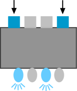
Figure 1: A box corresponding to a contextuality scenario.

In an ideal situation, it is generally assumed that behaviors must satisfy the non-disturbance condition, that states that whenever two contexts $\bm{\gamma}$ and $\bm{\gamma}^{\prime}$ overlap, the marginal $p^{\bm{\gamma}}_{\bm{\gamma}\cap\bm{\gamma}^{\prime}}$ for $\bm{\gamma}\cap\bm{\gamma}^{\prime}$ computed from the distribution for $\bm{\gamma}$ and the marginal $p^{\bm{\gamma}^{\prime}}_{\bm{\gamma}\cap\bm{\gamma}^{\prime}}$ for $\bm{\gamma}\cap\bm{\gamma}^{\prime}$ computed from the distribution for $\bm{\gamma}^{\prime}$ must coincide.

Definition III.3.

The non-disturbance set $\mathsf{ND}\left(\Upsilon\right)$ is the set of behaviors such that for any two intersecting contexts $\bm{\gamma}$ and $\bm{\gamma}^{\prime}$ the consistency relation $p^{\bm{\gamma}}_{\bm{\gamma}\cap\bm{\gamma}^{\prime}}=p^{\bm{\gamma}^{\prime}}_{\bm{\gamma}\cap\bm{\gamma}^{\prime}}$ holds.

We ask now if it is possible to define a distribution on the set $\mathcal{O}^{\mathcal{M}}$, which specifies assignment of outcomes to all measurements, in a way that the restrictions yield the probabilities specified by the behavior on all contexts in $\mathcal{C}$ Abramsky and Brandenburger, (2011).

Definition III.4.

A global section for $\mathcal{M}$ is a probability distribution $p_{\mathcal{M}}:\mathcal{O}^{\mathcal{M}}\rightarrow[0,1]$. A global section for a behaviour $\bm{B}\in\mathsf{ND}\left(\Upsilon\right)$ is a global section for $\mathcal{M}$ such that the marginal probability distribution defined by $p_{\mathcal{M}}$ in each context $\bm{\gamma}\in\mathcal{C}$ is equal to $p_{\bm{\gamma}}$. The behaviors for which there is a global section are called non-contextual. The set of all non-contextual behavior will be denoted by $\mathsf{NC}\left(\Upsilon\right)$

As an example, consider the scenario $\Upsilon$ containing three dicotomic measurements $\{x,y,z\}$ whith measurement $y$ compatible with the two others. Mathematically, $\Upsilon=\left(X,\mathcal{C},\mathcal{O}\right)$ with $\mathcal{O}=\left\{-1,1\right\}$, $\mathrm{X}=\left\{x,y,z\right\}$ and $\mathcal{C}=\left\{\{x,y\},\{y,z\}\right\}$. The graph representation of this scenario is shown in Fig. 2.

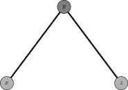
Figure 2: A compatibility scenario with three measurements $x,y,z$ and two contexts, $\left\{x,y\right\}$ and $\left\{y,z\right\}$.

In this scenario, a behavior consists in specifying probability distributions

$$p_{xy}(ab),\,\,a,b\in\{-1,1\}, \ \ \ \ p_{yz}(bc),\,\,b,c\in\{-1,1\}.$$ (3)

The non-disturbance condition demands that

$$p_{y}\left(b\right)\coloneqq\sum_{a}p_{xy}(ab)=\sum_{c}p_{yz}(bc)$$ (4)

and a behavior is non-contextual if there is a global probability distribution $p_{xyz}\left(abc\right)$ such that

$$p_{xy}(ab)=\sum_{c}p_{xyz}\left(abc\right), \ \ \ \ p_{yz}(bc)=\sum_{a}p_{xyz}\left(abc\right).$$ (5)

The set of objects in the resource theory of contextuality considered in this contribution is the set of non-disturbing boxes and the set of free objects is the set of non-contextual boxes in arbitrary compatibility scenarios with finite set of measurements and outcomes.

IV Free operations

IV.1 Pre-processing operations

We first consider compositions of the initial box $\bm{B}=\left(\mathcal{M},\mathcal{C},\mathcal{O}\right)$ with a non-contextual pre-processing box $\bm{B}_{\mathrm{PRE}}=\left(\mathcal{M}_{\mathrm{PRE}},\mathcal{C}_{\mathrm{PRE}},\mathcal{O}_{\mathrm{PRE}}\right)$ (see fig. 3). We demand that the output lights of $\bm{B}_{\mathrm{PRE}}$ be in one-to-one correspondence with the input buttons of $\bm{B}$ in such a way that if a set of lights $\bm{r}$ in $\bm{B}_{\mathrm{PRE}}$ can be on jointly, the corresponding buttons $\bm{\gamma}\left(\bm{r}\right)$ in $\mathcal{M}$ form a context of $\mathcal{C}$. This restriction guarantees that the composition will not associate outcomes that can be produced in box $\bm{B}_{\mathrm{PRE}}$ with buttons that can not be jointly pressed in the box $\bm{B}$, ensuring that the transformation is consistently defined. This operation results in a box $\mathcal{W}_{\mathrm{PRE}}(\bm{B})$ with input buttons $\mathcal{M}_{\mathrm{PRE}}$, compatibility graph $\mathcal{C}_{\mathrm{PRE}}$, and output lights $\mathcal{O}$. The behavior of $\mathcal{W}_{\mathrm{PRE}}(\bm{B})$ will be given by

$$p_{\bm{\beta}}\left(\bm{s}\right)=\sum_{\bm{r}}p_{\bm{\gamma}(\bm{r})}(\bm{s})p_{\bm{\beta}}(\bm{r})$$ (6)

where $\bm{\beta}$ is any context in $\mathcal{C}_{\mathrm{PRE}}$, $\bm{r}$ runs over the possible output lights associated with context $\bm{\beta}$ in box $\bm{B}_{\mathrm{PRE}}$, $\bm{\gamma}(\bm{r})\in\mathcal{C}$ is the context of box $\bm{B}$ corresponding to $\bm{r}$ and $\bm{s}$ is one of the possible set of output lights associated with context $\bm{\gamma}(\bm{r})$.

IV.2 Post-processing operations

We can also compose the initial box $\bm{B}$ with a non-contextual post-processing box $\bm{B}_{\mathrm{POST}}=\left(\mathcal{M}_{\mathrm{POST}},\mathcal{C}_{\mathrm{POST}},\mathcal{O}_{\mathrm{POST}}\right)$ (see fig. 3). Analogously, to ensure that the transformation is consistently defined, we demand that the output lights of $\bm{B}$ be in one-to-one correspondence with the input buttons of $\bm{B}_{\mathrm{POST}}$ in such a way that if a set of lights $\bm{s}$ in $\bm{B}_{\mathrm{POST}}$ can be on jointly, the corresponding buttons $\bm{\delta}\left(\bm{s}\right)$ in $\mathcal{M}_{\mathrm{POST}}$ are a context of $\mathcal{C}_{\mathrm{POST}}$. We have now a final box $\mathcal{W}_{\mathrm{POST}}(\bm{B})$ with input buttons $\mathcal{M}$, compatibility graph $\mathcal{C}$, and output lights $\mathcal{O}_{\mathrm{POST}}$. The behavior of $\mathcal{W}_{\mathrm{POST}}(\bm{B})$ will be given by

$$p_{\bm{\gamma}}\left(\bm{t}\right)=\sum_{\bm{s}}p_{\bm{\delta}(\bm{s})}(\bm{t})p_{\bm{\gamma}}(\bm{s})$$ (7)

where $\bm{\gamma}$ is any context in $\mathcal{C}$, $\bm{s}$ runs over the possible sets of output lights associated with context $\bm{\gamma}$ in box $\bm{B}$, $\bm{\delta}(\bm{s})\in\mathcal{C}_{\mathrm{POST}}$ is the context of box $\bm{B}_{\mathrm{POST}}$ corresponding to $\bm{s}$ and $\bm{t}$ is one of the possible output lights associated with context $\bm{\delta}(\bm{s})$.

(a)

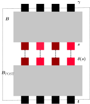
(b)

Figure 3: (a) A pre-processing operation that transforms the initial box $\bm{B}$ into the final box $\mathcal{W}_{\mathrm{PRE}}(\bm{B})$. When context $\bm{\beta}$ is chosen for box $\bm{B}_{\mathrm{PRE}}$ and outcome $\bm{r}$ is obtained, we have a corresponding context $\bm{\gamma}\left(\bm{r}\right)$ that is now pressed in box $\bm{B}$. If outcome $\bm{s}$ is obtained in the second box, we say that $\bm{s}$ was the outcome for context $\bm{\beta}$ in the final box. (b) A post-processing operation that transforms the initial box $\bm{B}$ into the final box $\mathcal{W}_{\mathrm{POST}}(\bm{B})$. When context $\bm{\gamma}$ is chosen for box $\bm{B}$ and outcome $\bm{s}$ is obtained, we have a corresponding context $\bm{\delta}(\bm{s})$ that is now pressed in box $\bm{B}_{\mathrm{POST}}$. If outcome $\bm{t}$ is obtained in the second box, we say that $\bm{t}$ was the outcome for context $\bm{\gamma}$ in the final box.

IV.3 Non-contextual Wirings

A non-contextual wiring is a composition of a pre-processing and a post-processing operation with the additional freedom that the behavior of the post-processing box can depend on the input $\bm{\beta}$ and output $\bm{r}$ of the pre-processing box. The behavior of the post-processing box is then of the form $p_{\bm{\delta}}\left(\bm{t}|\bm{\beta},\bm{r}\right),$ but in such a way that each output light of the post-processing box is causally influenced only by the inputs and outputs of the pre-processing box that are associated with it. This additional restriction is crucial in order not to create contextuality with the post-processing itself. To understand this restriction, consider a run of the wiring as shown in fig. 4.

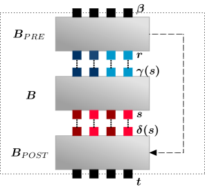
Figure 4: A non-contextual wiring $\mathcal{W}_{\mathrm{NC}}$ with respect to pre- and post-processing boxes $\bm{B}_{\mathrm{PRE}}$ and $\bm{B}_{\mathrm{POST}}$, respectively, mapping an initial box $\bm{B}$ into a final box $\mathcal{W}_{\mathrm{NC}}(\bm{B})$. The buttons and lights of $\mathcal{W}_{\mathrm{NC}}(\bm{B})$ are given by the buttons of $\bm{B}_{\mathrm{PRE}}$ and the lights of $\bm{B}_{\mathrm{POST}}$, respectively. Only the lights (buttons) of $\bm{B}$ of the same color can be on (pressed) at the same time. The behavior of $\bm{B}_{\mathrm{POST}}$ is causally influenced by $\bm{B}_{\mathrm{PRE}}$, but in a restricted way such that the statistics of each output light of $\bm{B}_{\mathrm{POST}}$ depends only on the buttons and lights of $\bm{B}_{\mathrm{PRE}}$ that are associated with it. As a result, if $\bm{B}$ is non-contextual so is $\mathcal{W}_{\mathrm{NC}}(\bm{B})$.

Let $\beta_{i}$ be an input button of $\bm{B}_{\mathrm{PRE}}$ in context $\bm{\beta}$ and $r_{i}$ be the associated outcome in $\bm{r}$. Let $\gamma_{i}$ be the input button in $\bm{B}$ associated to $r_{i}$ and $s_{i}$ be the corresponding outcome in $\bm{s}$. Let $\delta_{i}$ be the input button in $\bm{B}_{\mathrm{POST}}$ associated to $s_{i}$ and $t_{i}$ be the corresponding outcome in $\bm{t}$. The consistency conditions in the definition of pre and post-processing operations guarantee that all these input buttons and output lights are well defined (see Amaral et al., (2018) for details). We demand that

$$p_{\bm{\delta}}\left(\bm{t}|\bm{\beta},\bm{r}\right)=\sum_{\phi}p(\phi)\prod_{i}p_{\delta_{i}\left(s_{i}\right)}\left(t_{i}|\beta_{i},r_{i}\right)$$ (8)

where $\phi\in\Phi$ is an arbitrary additional variable, $p(\phi)$ is a probability distribution over $\Phi$, and $p_{\delta_{i}}\left(t_{i}|\beta_{i},r_{i}\right)$ is the probability of having outcome $t_{i}$ for button $\delta_{i}\left(s_{i}\right)$ on box $\bm{B}_{\mathrm{POST}}$ given $\phi$, $\beta_{i}$ and $r_{i}$. Fig. 5 shows an example where each set of buttons and lights has exactly two elements.

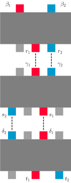
Figure 5: One round of the non-contextual wiring where context $\bm{\beta}=\left\{\beta_{1},\beta_{2}\right\}$ is chosen for box $\bm{B}_{\mathrm{PRE}}$, leading to the sequences of buttons and lights $\left(\beta_{1},r_{1},\gamma_{1},s_{1},\delta_{1},t_{1}\right)$ and $\left(\beta_{2},r_{2},\gamma_{2},s_{2},\delta_{2},t_{2}\right)$. The behavior of box $\bm{B}_{\mathrm{POST}}$ can depend on box $\bm{B}_{\mathrm{PRE}}$, but with the restriction that the probability of output $t_{1}$ for button $\gamma_{1}$ can depend only on $\beta_{1}$ and $r_{1}$ and the probability of output $t_{2}$ for button $\delta_{2}$ can depend only on $\beta_{2}$ and $r_{2}$, and hence $p_{\bm{\delta}\left(\bm{s}\right)}\left(\bm{t}|\bm{\beta},\bm{r}\right)=p_{\delta_{1}}\left(t_{1}|\beta_{1},r_{1}\right)\times p_{\delta_{2}}\left(t_{2}|\beta_{2},r_{2}\right)$. If we consider the situation in which button $\beta_{2}$ is pressed only after outcome $t_{1}$ is recorded, this restriction implies that the behavior of the post-processing box depends only on the sequence $\left(\beta_{2},r_{2},\gamma_{2},s_{2},\delta_{2},t_{2}\right)$ and the wiring has no memory of the previous round $\left(\beta_{1},r_{1},\gamma_{1},s_{1},\delta_{1},t_{1}\right)$. We want the set of free operations to be convex and hence we also allow for convex combinations of such instances, given by the sum over the variable $\phi$ in equation (8).

This composition defines a final box $\mathcal{W}_{\mathrm{NC}}\left(\bm{B}\right)$ with input buttons $\mathcal{M}_{\mathrm{PRE}}$, compatibility graph $\mathcal{C}_{\mathrm{PRE}}$, and output lights $\mathcal{O}_{\mathrm{POST}}$. The behavior of the final box will be given by

$$p_{\bm{\beta}}\left(\bm{t}\right)=\sum_{\bm{s},\bm{r}}p_{\bm{\delta}(\bm{s})}(\bm{t})p_{\bm{\gamma}(\bm{r})}(\bm{s})p_{\bm{\beta}}(\bm{r})$$ (9)

where $\bm{\beta}\in\mathcal{C}_{\mathrm{PRE}}$, $\bm{r}$ runs over the possible output lights associated with context $\bm{\beta}$ in box $\bm{B}_{\mathrm{PRE}}$, $\bm{\gamma}(\bm{r})\in\mathcal{C}$ is the context of box $\bm{B}$ corresponding to $\bm{r}$, $\bm{s}$ runs over the output lights associated with context $\bm{\gamma}(\bm{r})$, $\bm{\delta}(\bm{s})\in\mathcal{C}_{\mathrm{POST}}$ is the context of box $\bm{B}_{\mathrm{POST}}$ corresponding to $\bm{s}$, and $\bm{t}$ is one of the possible output lights associated with context $\bm{\delta}(\bm{s})$.

The set of all non-contextual wirings will be denoted by $\mathsf{NCW}$. Self-consistency of the theory requires that non-contextual wirings satisfy the following property, proven here for context with two buttons. The general case is completely analogous and a general proof can be found in the supplemental material of ref. Amaral et al., (2018).

Lemma IV.1 (Non-disturbance preservation).

The class of boxes $\mathsf{ND}$ is closed under all wirings in $\mathsf{NCW}$.

Proof.

Suppose that $\bm{\beta}=\left\{\beta_{1},\beta_{2}\right\}$. Since when one button is pressed exactly one light turns on, we have $\bm{r}=\left\{r_{1},r_{2}\right\}$, $\bm{\gamma}\left(\bm{r}\right)=\left\{\gamma_{1}\left(r_{1}\right),\gamma_{2}\left(r_{2}\right)\right\}$, $\bm{s}=\left\{s_{1},s_{2}\right\}$, $\bm{\delta}\left(\bm{s}\right)=\left\{\delta_{1}\left(s_{1}\right),\delta_{2}\left(s_{2}\right)\right\}$, as in fig. 5. We have that

$$\sum_{t_{2}}p_{\bm{\beta}}\left(\bm{t}\right) = \sum_{t_{2}}\sum_{\bm{r},\bm{s}}p_{\bm{\delta}\left(\bm{s}\right)}\left(\bm{t}\right)p_{\bm{\gamma}\left(\bm{r}\right)}\left(\bm{s}\right)p_{\bm{\beta}}\left(\bm{r}\right)$$ (10)

$$= \sum_{t_{2}}\sum_{\bm{r},\bm{s}}\sum_{\phi}p\left(\phi\right)p_{\delta_{1}\left(s_{1}\right)}\left(t_{1}|\beta_{1},r_{1},\phi\right)p_{\delta_{2}\left(s_{2}\right)}\left(t_{2}|\beta_{2},r_{2},\phi\right)p_{\bm{\gamma}\left(\bm{r}\right)}\left(\bm{s}\right)p_{\bm{\beta}}\left(\bm{r}\right)$$ (11)

$$= \sum_{\bm{r},\bm{s}}\sum_{\phi}p\left(\phi\right)p_{\delta_{1}\left(s_{1}\right)}\left(t_{1}|\beta_{1},r_{1},\phi\right)\left[\sum_{t_{2}}p_{\delta_{2}\left(s_{2}\right)}\left(t_{2}|\beta_{2},r_{2},\phi\right)\right]p_{\bm{\gamma}\left(\bm{r}\right)}\left(\bm{s}\right)p_{\bm{\beta}}\left(\bm{r}\right)$$ (12)

$$= \sum_{r_{1},r_{2},s_{1},s_{2}}\sum_{\phi}p\left(\phi\right)p_{\delta_{1}\left(s_{1}\right)}\left(t_{1}|\beta_{1},r_{1},\phi\right)p_{\bm{\gamma}\left(\bm{r}\right)}\left(\bm{s}\right)p_{\bm{\beta}}\left(\bm{r}\right)$$ (13)

$$= \sum_{r_{1},s_{1}}\sum_{\phi}p\left(\phi\right)p_{\delta_{1}\left(s_{1}\right)}\left(t_{1}|\beta_{1},r_{1},\phi\right)\sum_{r_{2},s_{2}}p_{\bm{\gamma}\left(\bm{r}\right)}\left(\bm{s}\right)p_{\bm{\beta}}\left(\bm{r}\right)$$ (14)

$$= \sum_{r_{1},s_{1}}\sum_{\phi}p\left(\phi\right)p_{\delta_{1}\left(s_{1}\right)}\left(t_{1}|\beta_{1},r_{1},\phi\right)p_{\gamma_{1}(r_{1})}(s_{1})\sum_{r_{2}}p_{\bm{\beta}}\left(\bm{r}\right)$$ (15)

$$= \sum_{r_{1},s_{1}}\sum_{\phi}p\left(\phi\right)p_{\delta_{1}\left(s_{1}\right)}\left(t_{1}|\beta_{1},r_{1},\phi\right)p_{\gamma_{1}(r_{1})}(s_{1})p_{\beta_{1}}\left(r_{1}\right)$$ (16)

$$= p_{\beta_{1}}\left(t_{1}\right).$$ (17)

∎

In addition, to give valid free operations, $\mathsf{NCW}$ must fulfill the following requirement, proven here for contexts with two buttons Amaral et al., (2018).

Theorem IV.1 (Non-contextuality preservation).

The class of boxes $\mathsf{NC}$ is closed under all wirings in $\mathsf{NCW}$.

Proof.

Non-conextuality of $\bm{B}_{\mathrm{PRE}}$, $\bm{B}$ and $B_{\mathrm{POST}}$ and condition (8) imply that

$$p_{\bm{\beta}}\left(\bm{r}\right) =\sum_{\xi}p\left(\xi\right)p_{\beta_{1}}\left(r_{1}|\xi\right)p_{\beta_{2}}\left(r_{2}|\xi\right),$$ (18)

$$p_{\bm{\gamma}\left(\bm{r}\right)}\left(\bm{s}\right) =\sum_{\psi}p\left(\psi\right)p_{\gamma_{1}\left(r_{1}\right)}\left(s_{1}|\psi\right)p_{\gamma_{2}\left(r_{2}\right)}\left(s_{2}|\psi\right),$$ (19)

$$p_{\bm{\delta}\left(\bm{s}\right)}\left(\bm{t}\right) =\sum_{\phi}p\left(\phi\right)p_{\delta_{1}\left(s_{1}\right)}\left(t_{1}|\beta_{1},r_{1},\phi\right)p_{\delta_{2}\left(r_{2}\right)}\left(t_{2}|\beta_{2},r_{2},\phi\right).$$ (20)

This in turn implies that

$$p_{\bm{\beta}}\left(\bm{t}\right) =\sum_{\bm{r},\bm{s}}p_{\bm{\delta}\left(\bm{s}\right)}\left(\bm{t}\right)p_{\bm{\gamma}\left(\bm{r}\right)}\left(\bm{s}\right)p_{\bm{\beta}}\left(\bm{r}\right)$$ (21)

$$=\sum_{\xi,\psi,\phi}\sum_{r_{1},r_{2},s_{1},s_{2}}p\left(\xi\right)p\left(\psi\right)p\left(\phi\right)p_{\delta_{1}\left(s_{1}\right)}\left(t_{1}|\beta_{1},r_{1},\phi\right)p_{\delta_{2}\left(r_{2}\right)}\left(t_{2}|\beta_{2},r_{2},\phi\right)$$

$$\hskip 90.00014pt\times p_{\gamma_{1}\left(r_{1}\right)}\left(s_{1}|\psi\right)p_{\gamma_{2}\left(r_{2}\right)}\left(s_{2}|\psi\right)p_{\beta_{1}}\left(r_{1}|\xi\right)p_{\beta_{2}}\left(r_{2}|\xi\right)$$ (22)

$$=\sum_{\bm{\psi}}p\left(\bm{\psi}\right)\left[\sum_{r_{1},s_{1}}p_{\delta_{1}\left(s_{1}\right)}\left(t_{1}|\beta_{1},r_{1},\phi\right)p_{\gamma_{1}\left(r_{1}\right)}\left(s_{1}|\psi\right)p_{\beta_{1}}\left(r_{1}|\xi\right)\right]$$

$$\hskip 90.00014pt\times\left[\sum_{r_{2},s_{2}}p_{\delta_{2}\left(r_{2}\right)}\left(t_{2}|\beta_{2},r_{2},\phi\right)p_{\gamma_{2}\left(r_{2}\right)}\left(s_{2}|\xi\right)p_{\beta_{2}}\left(r_{2}|\xi\right)\right]$$ (23)

$$=\sum_{\bm{\psi}}p\left(\bm{\psi}\right)p_{\beta_{1}}\left(t_{1}|\bm{\psi}\right)p_{\beta_{2}}\left(t_{2}|\bm{\psi}\right).$$ (24)

where $\bm{\psi}=\left(\xi,\psi,\phi\right).$ ∎

This proof is connected to the fact that the composition of any three independent non-contextual boxes yields a final box that is also non-contextual (with three independent non-contextual hidden variables). $\mathsf{NCW}$ is however more powerful than such compositions because the pre- and post-processing boxes here are not independent. Still, the restriction of eq. (8) enables non-contextuality preservation (see Amaral et al., (2018)). For space-like separated measurements, $\mathsf{NCW}$ reduces to local operations assisted by shared randomness, the canonical free operations of Bell non-locality Gallego et al., (2012); de Vicente, (2014); Gallego and Aolita, (2017). This also shows that non-contextual wirings is not the largest set of free operations for contextuality, since in the particular case of Bell scenarios it is known that local operations assisted by shared randomness is not the largest set of free operations of non-locality. However, we still lack an explicit parametrization for a larger set of free operations for contextuality, and we restrict throughout to the class of non-contextual wirings, unless stated otherwise, since this is the class for which we have a friendly parametrization with a clear physical interpretation.

Product and controlled choice of boxes

We consider now two different ways of combining independent boxes $\bm{B}_{1}=\left(\mathcal{M}_{1},\mathcal{C}_{1},\mathcal{O}_{1}\right)$ and $\bm{B}_{2}=\left(\mathcal{M}_{2},\mathcal{C}_{2},\mathcal{O}_{2}\right)$. First we define the box $\bm{B}_{1}\otimes\bm{B}_{2}$, called the product of $\bm{B}_{1}$ and $\bm{B}_{2}$, as the box such that each of its contexts is given by $\bm{\gamma}=\bm{\gamma}_{1}\cup\bm{\gamma}_{2}$, with $\bm{\gamma}_{i}\in\mathcal{C}_{i}$, that is, each context in the final box $\bm{B}_{1}\otimes\bm{B}_{2}$ consists of a choice of context for box $\bm{B}_{1}$ and a choice of context for $\bm{B}_{2}$ . The behavior of this box is

$$p_{\bm{\gamma}_{1}\cup\bm{\gamma}_{2}}\left(\bm{s}_{1},\bm{s}_{2}\right)=p_{\bm{\gamma}_{1}}\left(\bm{s}_{1}\right)p_{\bm{\gamma}_{2}}\left(\bm{s}_{2}\right).$$ (25)

Figure 6: The box $\bm{B}_{1}\otimes\bm{B}_{2}$ for which each context consists of a choice of context for box $\bm{B}_{1}$ and a choice of context for $\bm{B}_{2}$.

We can also define the box $\bm{B}_{1}\&\bm{B}_{2}$, called the controlled choice of $\bm{B}_{1}$ and $\bm{B}_{2}$, as the box such that $\mathcal{C}=\mathcal{C}_{1}\cup\mathcal{C}_{2}$, that is, each context in the final box $\bm{B}_{1}\&\bm{B}_{2}$ consists of a choice of context for box $\bm{B}_{1}$ or a choice of context for $\bm{B}_{2}$. The behavior of this box is a juxtaposition of a behavior for box $\bm{B}_{1}$ and a behavior for $\bm{B}_{2}$.

(a)

(b)

Figure 7: The box $\bm{B}_{1}\&\bm{B}_{2}$ for which each context consists of a choice of context for box $\bm{B}_{1}$ or a choice of context for $\bm{B}_{2}$.

V Quantifiers

The essential requirement for a function to be a valid measure of contextuality is that it is monotonous (i.e. non-increasing) under the set of non-contextual wirings.

Definition V.1.

A function $Q:\mathsf{ND}\left(\Upsilon\right)\rightarrow\mathds{R}$ is a contextuality monotone for the resource theory of contextuality defined by non-contextual wirings if

$$Q\left[\mathcal{W}\left(B\right)\right]\leq Q\left(B\right)$$ (26)

for every $\mathcal{W}\in\mathsf{NWC}$.

Besides monotonicity under free operations, other properties of a monotone $Q$ are also desirable Horodecki et al., (2015); Abramsky et al., (2017):

1. Faithfullness: For all $\bm{B}\in\mathsf{NC}(\Upsilon)$, $Q\left(\bm{B}\right)=0$.

2. Preservation under reversible operations: If $\mathcal{T}\in\mathcal{W}$ is reversible, then

   $$Q\left(\mathcal{T}\left(\bm{B}\right)\right)=Q\left(\bm{B}\right).$$ (27)

3. Additivity: Given two independent boxes $\bm{B}_{1}$ and $\bm{B}_{2}$ we require:

   $$Q\left(\bm{B}_{1}\otimes\bm{B}_{2}\right)\leq Q\left(\bm{B}_{1}\right)+Q\left(\bm{B}_{2}\right).$$ (28)

   $$Q\left(\bm{B}_{1}\&\bm{B}_{2}\right)\leq Q\left(\bm{B}_{1}\right)+Q\left(\bm{B}_{2}\right).$$ (29)

4. Convexity: If a behavior can be written as $\bm{B}=\sum_{i}\pi_{i}\bm{B}^{i}$, where $\pi_{i}\in[0,1]$ and each $\bm{B}^{i}$ is a behavior for the same scenario, then

   $$Q\left(\bm{B}\right)\leq\sum_{i}\pi_{i}Q\left(\bm{B}^{i}\right).$$ (30)

5. Continuity: $Q\left(\bm{B}\right)$ should be a continuous function of $\bm{B}$.

In what follows we exhibit a number of monotones for different resource theories of contextuality and list which of the properties above they satisfy.

V.1 Entropic Contextuality Quantifiers

V.1.1 Relative entropy of contextuality

In ref. Grudka et al., (2014), the authors also introduce two measures of contextuality based directly on the notion of relative entropy distance, also called the Kullback-Leibler divergence. Given two probability distributions $p$ and $q$ in a sample space $\Omega$, the Kullback-Leiber divergence between $p$ and $q$

$$D_{\mathrm{KL}}(p\|q)=\sum_{i\in\Omega}p(i)\,\log\frac{p(i)}{q(i)}$$ (31)

is a measure of the difference between the two probability distributions.

Definition V.2.

The Relative Entropy of Contextuality of a behavior $\bm{B}$ is defined as

$$E_{max}\left(\bm{B}\right)=\min_{\bm{B}^{NC}\in\mathsf{NC}}\ \ \max_{\pi}\ \ \sum_{\bm{\gamma}\in\mathcal{C}}\ \pi\left(\bm{\gamma}\right)D_{\mathrm{KL}}\left(p_{\bm{\gamma}}\middle\|p^{NC}_{\bm{\gamma}}\right),$$ (32)

where the minimum is taken over all non-contextual behaviors $\bm{B}^{NC}=\left\{p^{NC}_{\bm{\gamma}}\right\}$ and the maximum is taken over all probability distributions $\pi$ defined on the set of contexts $\mathcal{C}$. The Uniform Relative Entropy of Contextuality of $\bm{B}$ is defined as

$$E_{u}\left(\bm{B}\right)=\frac{1}{N}\min_{\bm{B}^{NC}\in\mathsf{NC}}\ \ \sum_{\bm{\gamma}\in\mathcal{C}}\ D_{\mathrm{KL}}\left(p_{\bm{\gamma}}\middle\|p^{NC}_{\bm{\gamma}}\right),$$ (33)

where $N=\left|\mathcal{C}\right|$ is the number of contexts in $\mathcal{C}$ and, once more, the minimum is taken over all non-contextual behaviors $\bm{B}^{NC}=\left\{p^{NC}_{\bm{\gamma}}\right\}$.

In reference Amaral et al., (2018) it is shown that $E_{max}$ is a monotone under non-contextual wirings. The quantity $E_{u}$, however, is not a monotone under the complete class of non-contextual wirings, as shown in Ref. Gallego and Aolita, (2017) for the special class of Bell scenarios. Nonetheless, it is a monotone under a broad class of such operations. More specifically, it is monotone under post-processing operations and under a subclass of pre-processing operations (see ref. Amaral and Cunha, (2017)).

Theorem V.1.

The following properties are valid for the contextuality quantifiers based on relative entropy:

1. $E_{max}$ is a contextuality monotone for the resource theory of contextuality defined by non-contextual wirings;

2. $E_{u}$ is a contextuality monotone for the resource theory of contextuality defined by post-processing operations and a subclass of pre-processing operations;

3. $E_{max}$ and $E_{u}$ are faithful, additive, convex, continuous, and preserved under relabellings of inputs and outputs.

The proof of this result can be found in refs. Grudka et al., (2014); Horodecki et al., (2015); Amaral and Cunha, (2017).

V.2 Geometric Contextuality Quantifiers

We now introduce contextuality monotones based on the distance $\ell_{1}$, in contrast with the previous defined quantifiers which are based on entropic distances.

Definition V.3.

The $\ell_{1}$-max contextuality distance of a behavior $\bm{B}$ is defined as

$$\mathcal{D}_{max}\left(\bm{B}\right)=\min_{\bm{B}^{NC}\in\mathsf{NC}}\max_{\pi}\sum_{\bm{\gamma}\in\mathcal{C}}\ \pi\left(\bm{\gamma}\right)\ \sum_{\bm{s}}\left|p_{\bm{\gamma}}\left(\bm{s}\right)-p^{NC}_{\bm{\gamma}}\left(\bm{s}\right)\right|,$$ (34)

where the minimum is taken over all non-contextual behaviors $\bm{B}^{NC}=\left\{p^{NC}_{\bm{\gamma}}\right\}$ and the maximum is taken over all over all probability distributions $\pi$ defined over the set of contexts $\mathcal{C}$. The $\ell_{1}$-uniform contextuality distance of a behavior $B$ is defined as

$$\mathcal{D}_{u}\left(\bm{B}\right)=\frac{1}{N}\min_{\bm{B}^{NC}\in\mathsf{NC}}\sum_{\bm{\gamma}\in\mathcal{C}}\sum_{\bm{s}}\left|p_{\bm{\gamma}}\left(\bm{s}\right)-p^{NC}_{\bm{\gamma}}\left(\bm{s}\right)\right|,$$ (35)

where $N=\left|\mathcal{C}\right|$ is the number of contexts in $\mathcal{C}$.

For detailed discussion of these contextuality quantifiers see ref. Amaral and Cunha, (2017) and, for the special class of Bell scenarios, ref. Brito et al., (2018)).

Theorem V.2.

The following properties are satisfied:

1. $\mathcal{D}_{max}$ is a contextuality monotone for the resource theory of contextuality defined by the non-contextual wiring operations;

2. $\mathcal{D}_{u}$ is a contextuality monotone for the resource theory of contextuality defined by post-processing operations and a subclass of pre-processing operations;

3. $\mathcal{D}_{u}$ and $\mathcal{D}_{max}$ are faithful, additive, convex, continuous, and preserved under relabellings of inputs and outputs.

4. $\mathcal{D}_{u}$ can be computed using linear programming.

This result is proven in refs. Amaral and Cunha, (2017); Brito et al., (2018). It shows that while $\mathcal{D}_{max}$ is a proper contextuality monotone under the entire class of non-contextual wirings, $D_{u}$ are more suitable when the set of allowed free operations preserves the scenario under consideration. Other distances defined in the set $\mathsf{ND}$ can also be used in place of the $\ell_{1}$ distance. The above results are also valid for any $\ell_{p}$ distance.

V.3 Contextual Fraction

A contextuality quantifier based on the intuitive notion of what fraction of a given behavior admits a non-contextual description was introduced in refs. Abramsky and Brandenburger, (2011); Amselem et al., (2012). Several properties of this quantifier were further discussed in Ref. Abramsky et al., (2017).

Definition V.4.

The contextual fraction of a behavior $\bm{B}$ is defined as

$$\mathcal{CF}\left(\bm{B}\right)=\min\left\{\lambda\left|\bm{B}=\lambda\bm{B}^{\prime}+\left(1-\lambda\right)\bm{B}^{NC}\right.\right\},$$ (36)

where the minimum is taken over all decompositions of $\bm{B}$ as a convex sum of a non-contextual behavior $\bm{B}^{NC}$ and an arbitrary behavior $\bm{B}^{\prime}$.

Theorem V.3.

The contextual fraction is a monotone under all linear operations that preserve the non-contextual set $\mathsf{NC}$.

Proof.

Let $\mathcal{T}$ be a linear operation over the set of behaviors such that

$$\mathcal{T}\left(\mathsf{NC}\right)\subset\mathsf{NC}.$$ (37)

Given a behavior $\bm{B}$, let $\bm{B}=\lambda\bm{B}^{\prime}+\left(1-\lambda\right)\bm{B}^{NC}$ be the decomposition of $\bm{B}$ achieving the minimum in eq. (36), that is, $\mathcal{CF}\left(\bm{B}\right)=\lambda$. Then

$$\mathcal{T}\left(\bm{B}\right) = \mathcal{T}\left(\lambda\bm{B}^{\prime}+\left(1-\lambda\right)\bm{B}^{NC}\right)$$ (38)

$$= \lambda\mathcal{T}\left(\bm{B}^{\prime}\right)+\left(1-\lambda\right)\mathcal{T}\left(\bm{B}^{NC}\right).$$ (39)

Since $\mathcal{T}\left(\bm{B}^{NC}\right)$ is a non-contextual behavior, we conclude that

$$\mathcal{CF}\left(\mathcal{T}\left(\bm{B}\right)\right)\leq\lambda=\mathcal{CF}\left(\bm{B}\right).$$ (40)

∎

Proposition V.1.

The contextual fraction satisfies:

1. The contextual fraction is faithful, convex and continuous;

2. $\mathcal{CF}\left(\bm{B}_{1}\&\bm{B}_{2}\right)\leq\max_{i}\mathcal{CF}\left(\bm{B}_{i}\right)$;

3. $\mathcal{CF}\left(\bm{B}_{1}\otimes\bm{B}_{2}\right)\leq\mathcal{CF}\left(\bm{B}_{1}\right)+\mathcal{CF}\left(\bm{B}_{2}\right)-\mathcal{CF}\left(\bm{B}_{1}\right)\mathcal{CF}\left(\bm{B}_{2}\right)$;

4. The contextual fraction can be calculated via linear programming.

The proof of these results can be found in Ref. Abramsky et al., (2017).

VI Contextuality as a resource

In this contribution we have defined the set of free objects using an abstract mathematical characterization of noncontextuality, but a resource theory of contextuality will exhibit its true power when applied to operational applications of this phenomenon. Contextuality has been identifyed as a possible resource for quantum advantages in different schemes and in this section we review some of the recent results.

Contextuality and random number generation

The generation of genuine randomness is still a challenging task as true random numbers can never be generated with classical systems, for which a deterministic description, in principle, always exists. For quantum system that exhibit contextuality, a deterministic description that is independent on the choice of measurement settings is impossible, thus opening the door for the generation of genuine random numbers. This was indeed achieved in refs. Pironio et al., (2010); Um et al., (2013) where the violation of Bell and non-contextuality inequalities where used directly to compute a lower bound on the min-entropy of the outcomes, thus guaranteeing randomness of the string of output bits. This string can then be processed using classical algorithms to distill genuine random numbers. It is interesting to note that the quantum system in ref. Um et al., (2013) is a qutrit, which shows that randomness can be generated without the need of using costly quantum resources such as entanglement. This allows for easier implementation and significantly higher generation rate of random strings.

Contextuality and models of quantum computation with state injection

Quantum computation with state injection (QCSI) Bravyi and Kitaev, (2005) is a scheme composed of a free part consisting of quantum circuits with restricted set of states, unitaries and measurements (generally restricted to be that of the stabilizer formalism) in which quantum computation universality is achieved by the injection of special resource states, called magic states. These special states are usually distilled from many copies of noisy states through a procedure called magic state distillation.

To understand the source of quantum advantage in these schemes we need to understand what is precisely the quantum property that allows for magic state distillation. In ref. Veitch et al., (2012), it was shown that for a special choice of Wigner function representation of qudits with prime $d$, its positivity implied the existence of an efficient classical simulation of the state, which in turn implied that this state is not useful for magic state distillation. This result was later explored in ref. Howard et al., (2014), which exhibited a contextuality scenario based on the set of restricted measurements for which non-contextuality is equivalent to negativity of the Wigner function. This shows that contextuality with respect to this scenario is a necessary ingredient for magic state distillation.

This result does not easily generalizes to quibt systems Bermejo-Vega et al., (2017); Lillystone et al., (2018), where both the definition of the Wigner function and the presence of state independent contextuality with respect to the restricted measurements poses an obstacle to the recognition of contextuality as a resource. Several attempts to establish contextuality as a resource in qubit stabilizer sub-theory have been done so by further restricting to non-contextual subsets of operations within the qubit stabilizer sub-theory. In ref. Delfosse et al., (2015), the authors restrict to qubits with real density matrices (rebits) and define a Wigner function for $n$ rebits that is consistent with the restricted stabilizer formalism. With this construction they are able to prove that there is a real QCSI schemes in which universal quantum computation is only possible in the presence of contextuality. In ref. Raussendorf et al., (2017), the authors show that if non-negative Wigner functions remain non-negative under free measurements, then contextuality and Wigner function negativity are necessary resources for universal quantum computation on these schemes. The result on contextuality is however strictly stronger than the result on Wigner functions, since different from the qudit case Delfosse et al., (2017), qubit magic states can have negative Wigner functions but still be non-contextual. These results where later generalized in ref. Bermejo-Vega et al., (2017), that shows that if the set of available measurements in the scheme is such that there exists a quantum states that does not exhibit contextuality, then contextuality is a necessary resource for universal quantum computation on these schemes.

Contextuality and measurement based quantum computation

A $\ell_{d}$-measurement-based quantum computation ($\ell_{d}$-MBQC) Raussendorf et al., (2003) consists of a $n$-site correlated resource state and a control classical computer with restricted computational power. Each site receives the information of a measurement setting to be performed in its system, encoded as an element of $\mathds{Z}_{d}$, with $d=p^{r}$ and $p$ prime, and returns the outcome of the measurement also encoded as an element of $\mathds{Z}_{d}$. No communication between sites is allowed during the computation. The control computer post-processes the measurement outcomes linearly to produce the output of the computation.

For $d=2$ it was shown in ref. Anders and Browne, (2009) that nonlinear Boolean functions can be computed with $\ell_{2}$-MBQC with a resource state constructed from a proof of contextuality based on Mermin’s GHZ paradox. It was then shown in ref. Raussendorf, (2013) that deterministic computation of any nonlinear Boolean function with $\ell_{2}$-MBQC implies that the contextual fraction of the corresponding behavior is equal to one. For probabilistic computation, $\ell_{2}$-MBQC which compute a non-linear Boolean function with high probability are necessarily contextual. Ref. Oestereich and Galvão, (2017) proves that bipartite non-local behaviors in the CHSH scenario and behaviors with arbitrarily small violation of a multi-partite GHZ non-contextuality inequality suffice for reliable classical computation, that is, for the evaluation of any Boolean function with success probability bounded away from $\frac{1}{2}$.

These results were later connected with the contextual fraction of the resource state with respect to the available measurements in the computation Abramsky et al., (2017). Let $f$ be a Boolean function and consider an $\ell_{2}$-MBQC that uses the behavior $\bm{B}$ to compute $f$ with average success probability $p_{S}$ overall possible inputs, and corresponding average failure probability $p_{F}=1-p_{S}$. Then

$$p_{F}\geq\left(1-\mathcal{CF}\left(\bm{B}\right)\right)\nu\left(f\right),$$ (41)

where $\nu\left(f\right)$ is the average distance of $f$ to the closest $\mathds{Z}_{2}$-linear function.

In the qudit case, however, examples of non-contextual $\ell_{d}$-MBQCs with local dimension $d\geq 3$ that evaluate nonlinear functions can be found Frembs et al., (2018). Nevertheless, it is still possible to connect contextuality with quantum advantages. In this direction, ref. Hoban et al., (2011) shows that the evaluation of a sufficiently high order polynomial function on a multi-qudit system provides a proof of contextuality. This problem was also investigated in ref. Frembs et al., (2018), that besides reproducing the result of Hoban et al., (2011), emphasised the distinctive role of contextuality in individual sites versus strong correlations between the sites.

Memory cost of simulating contextuality

Contextuality can be simulated by classical models with memory and the efficiency of such simulations can help understand the difference between quantum and classical systems. In any such simulation, the system changes between different internal states during the measurement sequence. These states, drawn from a classical state space $\Lambda$, can be considered as memory and define the spatial complexity of the simulation. The model in which the cardinality of $\Lambda$ is minimum is memory-optimal and defines the memory cost of the simulation.

In refs. Kleinmann et al., (2011); Fagundes and Kleinmann, (2017) the authors study the memory cost of simulating quantum contextuality in the Peres-Mermim scenario and show that three internal states are necessary for a perfect simulation of quantum behaviors. This shows that reproducing the results of sequential measurements on a two-qubit system requires more memory than the information-carrying capacity of the system, given by the Holevo bound. In ref. Karanjai et al., (2018) it is shown that contextuality in a quantum sub-theory puts a lower bound on the cardinality of the state space used in any classical simulation of this sub-theory. As a consequence of their result, the authors prove that the minimum amount of bits necessary to simulate the $n$-qubit stabilizer sub-theory grows quadratically with $n$, in contrast with the qudit case with $d$ an odd prime Delfosse et al., (2017), where an efficient simulation that scales linearly in $n$ can be constructed from a particular choice of Wigner representation, which is always positive for stabilizer states.

VII Conclusion

In this contribution, we reviewed some of the recent developments towards a unified resource theory for contextuality. Although these results highlight contextuality as a possible operational resource, the understanding of the connection of these constructions with practical applications is still in its infancy. This is the most important and the most challenging ingredient in a resource theory. Other important question regarding contextuality as a resource remain open, such as the possibility of contextuality distillation, the role of catalysts, conversion rates and the possibility of finding an explicit parametrization of larger classes of free operations for contextuality. It is also important to investigate the role of other forms of non-classicality in quantum advantage Duarte and Amaral, (2018); Mansfield and Kashefi, (2018) and, although quantifiers can be adapted to the contextuality-by-default framework of ref. Dzhafarov et al., (2016), it is still an open problem to find a version of the non-contextual wirings to this extended notion of contextuality.

We point out that although the main application of a resource theory is to understand the role of a physical property as an operational resource, this construction can be interesting on its own and it can give insight about the physical property under consideration. For example, in ref. Duarte et al., (2018) the authors use contextuality quantifiers to explore the geometry of the set of behaviors, finding the approximate relative volume of the non-contextual set in relation to the non-disturbing set.

Acknowledgments

The author thanks Adán Cabello, Ehtibar Dzhafarov, Emily Tyhurst, Ernesto Galvão, Jan-Åke Larsson, Jingfang Zhou, Leandro Aolita, Marcelo Terra Cunha, Paweł Horodecki, Paweł Kurzyński, Rui Soares Barbosa, Samsom Abramsky, Shane Mansfield and all the participants of the Winer Memorial Lectures at Purdue University for valuable discussions. The author thanks Ehtibar Dzhafarov, Maria Kon, and Víctor H. Cervantes for the organization of the event and Purdue University for its support and hospitality. The author acknowledges financial support from the Brazilian ministries and agencies MEC and MCTIC, INCT-IQ, FAPEMIG, and CNPq Universal grant n. 431443/2018-1.

References

- Abramsky and Brandenburger, (2011) Abramsky, A. and Brandenburger, A. (2011). The sheaf-theoretic structure of non-locality and contextuality. New Journal of Physics, 13(113036).
- Abramsky et al., (2017) Abramsky, S., Barbosa, R. S., and Mansfield, S. (2017). Contextual Fraction as a Measure of Contextuality. Physical Review Letters, 119(5):50504.
- Amaral et al., (2018) Amaral, B., Cabello, A., Cunha, M. T., and Aolita, L. (2018). Noncontextual Wirings. Physical Review Letters, 120(13).
- Amaral and Cunha, (2018) Amaral, B. and Cunha, M. (2018). On Graph Approaches to Contextuality and their Role in Quantum Theory. SpringerBriefs in Mathematics. Springer International Publishing.
- Amaral and Cunha, (2017) Amaral, B. and Cunha, M. T. (2017). On geometrical aspects of the graph approach to contextuality. arxiv:, quantum-ph.
- Amselem et al., (2012) Amselem, E., Danielsen, L. E., López-Tarrida, A. J., Portillo, J. R., Bourennane, M., and Cabello, A. (2012). Experimental Fully Contextual Correlations. Physical Review Letters, 108(20):200405.
- Anders and Browne, (2009) Anders, J. and Browne, D. E. (2009). Computational Power of Correlations. Physical Review Letters, 102(5):050502.
- Arvidsson-Shukur et al., (2019) Arvidsson-Shukur, D. R. M., Halpern, N. Y., Lepage, H. V., Lasek, A. A., Barnes, C. H. W., and Lloyd, S. (2019). Contextuality Provides Quantum Advantage in Postselected Metrology.
- Bermejo-Vega et al., (2017) Bermejo-Vega, J., Delfosse, N., Browne, D. E., Okay, C., and Raussendorf, R. (2017). Contextuality as a Resource for Models of Quantum Computation with Qubits. Physical Review Letters, 119(12).
- Bharti et al., (2018) Bharti, K., Ray, M., Varvitsiotis, A., Warsi, N. A., Cabello, A., and Kwek, L.-C. (2018). Robust self-testing of quantum systems via noncontextuality inequalities.
- Bravyi and Kitaev, (2005) Bravyi, S. and Kitaev, A. (2005). Universal quantum computation with ideal Clifford gates and noisy ancillas. Physical Review A - Atomic, Molecular, and Optical Physics, 71(2).
- Brito et al., (2018) Brito, S. G. A., Amaral, B., and Chaves, R. (2018). Quantifying Bell nonlocality with the trace distance. Physical Review A, 97(2).
- Coecke et al., (2016) Coecke, B., Fritz, T., and Spekkens, R. W. (2016). A mathematical theory of resources. Information and Computation, 250:59–86.
- de Vicente, (2014) de Vicente, J. I. (2014). On nonlocality as a resource theory and nonlocality measures. Journal of Physics A: Mathematical and Theoretical, 47(42):424017.
- Delfosse et al., (2015) Delfosse, N., Allard Guerin, P., Bian, J., Raussendorf, R., Guerin, P. A., Bian, J., and Raussendorf, R. (2015). Wigner Function Negativity and Contextuality in Quantum Computation on Rebits. Physical Review X, 5(2):21003.
- Delfosse et al., (2017) Delfosse, N., Okay, C., Bermejo-Vega, J., Browne, D. E., and Raussendorf, R. (2017). Equivalence between contextuality and negativity of the wigner function for qudits. New Journal of Physics, 19(12):123024.
- Duarte and Amaral, (2018) Duarte, C. and Amaral, B. (2018). Resource theory of contextuality for arbitrary prepare-and-measure experiments. Journal of Mathematical Physics, 59(6):062202.
- Duarte et al., (2018) Duarte, C., Brito, S., Amaral, B., and Chaves, R. (2018). Concentration phenomena in the geometry of bell correlations. Physical Review A, 98:062114.
- Dzhafarov et al., (2016) Dzhafarov, E. N., Kujala, J. V., and Cervantes, V. H. (2016). Contextuality-by-Default: A Brief Overview of Ideas, Concepts, and Terminology. In Atmanspacher, H., Filk, T., and Pothos, E., editors, Quantum Interaction, pages 12–23, Cham. Springer International Publishing.
- Fagundes and Kleinmann, (2017) Fagundes, G. and Kleinmann, M. (2017). Memory cost for simulating all quantum correlations from the Peres-Mermin scenario. Journal of Physics A: Mathematical and Theoretical, 50(32).
- Frembs et al., (2018) Frembs, M., Roberts, S., and Bartlett, S. D. (2018). Contextuality as a resource for measurement-based quantum computation beyond qubits. New Journal of Physics, 20(10):103011.
- Gallego and Aolita, (2017) Gallego, R. and Aolita, L. (2017). Nonlocality free wirings and the distinguishability between Bell boxes. Physical Review A, 95(3):32118.
- Gallego et al., (2012) Gallego, R., Würflinger, L. E., Acín, A., and Navascués, M. (2012). Operational Framework for Nonlocality. Physical Review Letters, 109(7):70401.
- Grudka et al., (2014) Grudka, A., Horodecki, K., Horodecki, M., Horodecki, P., Horodecki, R., Joshi, P., Kłobus, W., and Wójcik, A. (2014). Quantifying Contextuality. Physical Review Letters, 112:120401.
- Hoban et al., (2011) Hoban, M. J., Wallman, J. J., and Browne, D. E. (2011). Generalized Bell-inequality experiments and computation. Physical Review A - Atomic, Molecular, and Optical Physics, 84(6).
- Horodecki et al., (2015) Horodecki, K., Grudka, A., Joshi, P., Kłobus, W., and Łodyga, J. (2015). Axiomatic approach to contextuality and nonlocality. Physical Review A, 92:32104.
- Howard et al., (2014) Howard, M., Wallman, J., Veitch, V., and Emerson, J. (2014). Contextuality supplies the /‘magic/’ for quantum computation. Nature, 510(7505):351–355.
- Karanjai et al., (2018) Karanjai, A., Wallman, J. J., and Bartlett, S. D. (2018). Contextuality bounds the efficiency of classical simulation of quantum processes.
- Kleinmann et al., (2011) Kleinmann, M., Gühne, O., Portillo, J. R., Larsson, J.-Å., and Cabello, A. (2011). Memory cost of quantum contextuality. New Journal of Physics, 13(11):113011.
- Kochen and Specker, (1967) Kochen, S. and Specker, E. (1967). The Problem of Hidden Variables in Quantum Mechanics. J. Math. Mech., 17(1):59–87.
- Lillystone et al., (2018) Lillystone, P., Wallman, J. J., and Emerson, J. (2018). Contextuality and The Single-Qubit Stabilizer Formalism.
- Mansfield and Kashefi, (2018) Mansfield, S. and Kashefi, E. (2018). Quantum Advantage from Sequential-Transformation Contextuality. Physical Review Letters.
- (33) Note1. We give more details below for the case of contextuality and the reader can find the general case in ref. Coecke et al., (2016).
- (34) Note2. The average distance between two Boolean functions is given by .
- Oestereich and Galvão, (2017) Oestereich, A. L. and Galvão, E. F. (2017). Reliable computation from contextual correlations. Physical Review A, 96(6).
- Pironio et al., (2010) Pironio, S., Acín, A., Massar, S., de la Giroday, A. B., Matsukevich, D. N., Maunz, P., Olmschenk, S., Hayes, D., Luo, L., Manning, T. A., and Monroe, C. (2010). Random numbers certified by {B}ell’s theorem. Nature, 464(7291):1021–1024.
- Raussendorf, (2013) Raussendorf, R. (2013). Contextuality in measurement-based quantum computation. Physical Review A, 88(2):22322.
- Raussendorf et al., (2003) Raussendorf, R., Browne, D. E., and Briegel, H. J. (2003). Measurement-based quantum computation on cluster states. Physical Review A, 68(2):022312.
- Raussendorf et al., (2017) Raussendorf, R., Browne, D. E., Delfosse, N., Okay, C., and Bermejo-Vega, J. (2017). Contextuality and Wigner-function negativity in qubit quantum computation. Physical Review A, 95(5).
- Saha et al., (2017) Saha, D., Horodecki, P., and Pawłowski, M. (2017). State independent contextuality advances one-way communication. arXiv, 1708.04751.
- Schmid et al., (2018) Schmid, D., Spekkens, R. W., and Wolfe, E. (2018). All the noncontextuality inequalities for arbitrary prepare-and-measure experiments with respect to any fixed set of operational equivalences. Physical Review A, 97:062103.
- Um et al., (2013) Um, M., Zhang, X., Zhang, J., Wang, Y., Yangchao, S., Deng, D. L., Duan, L., and Kim, K. (2013). Experimental Certification of Random Numbers via Quantum Contextuality. Scientific Reports, 3(1627).
- Veitch et al., (2012) Veitch, V., Ferrie, C., Gross, D., and Emerson, J. (2012). Negative quasi-probability as a resource for quantum computation. New Journal of Physics, 14(11):113011.