Robust Alignment for Panoramic Stitching
via An Exact Rank Constraint

Abstract

We study the problem of image alignment for panoramic stitching. Unlike most existing approaches that are feature-based, our algorithm works on pixels directly, and accounts for errors across the whole images globally. Technically, we formulate the alignment problem as rank-1 and sparse matrix decomposition over transformed images, and develop an efficient algorithm for solving this challenging non-convex optimization problem. The algorithm reduces to solving a sequence of subproblems, where we analytically establish exact recovery conditions, convergence and optimality, together with convergence rate and complexity. We generalize it to simultaneously align multiple images and recover multiple homographies, extending its application scope towards vast majority of practical scenarios. Experimental results demonstrate that the proposed algorithm is capable of more accurately aligning the images and generating higher quality stitched images than state-of-the-art methods.

I Introduction

Panoramic stitching refers to the process of stitching several images together, assuming these images contain pairwise overlapping regions. Despite their variety, panoramic stitching algorithms generally follow the same pipelines [1]: first, estimate the parametric correspondences between input images, and then warp them towards a common canvas; this step is called alignment. Second, compose these aligned images together deliberately to conceal visual artifacts; this step is called stitching. Afterwards, several post-processing steps can be incorporated to further improve visual quality. Among these procedures, alignment serves as an essential step since properly aligned images can significantly reduce the burden of subsequent procedures. Besides, other applications such as object recognition can greatly benefit from more accurately aligned images [2, 3].

I-A Related Previous Work

Broadly speaking, alignment methods could be divided into two categories: pixel-based vs feature-based [1]. Pixel-based approaches typically estimate a dense correspondence field per pixel, while feature-based approaches generally rely on feature extraction, detection and matching. Despite extensive studies about pixel-based approaches [4, 5, 6, 7] especially in the early stage of image alignment, nowadays feature-based methods are much more widely used since pixel-based methods require close initializations under large displacements. To enhance the alignment accuracy of feature-based methods, a post-processing strategy called bundle adjustment [8] is usually performed.

In the seminal work of [9], a fully automated panorama system called AutoStitch is introduced. It employs a SIFT [10]-based alignment technique, followed by RANSAC [11] and probabilistic matching verification to enhance robustness. In a natural evolution of panoramic stitching, it was observed that a single homography motion model is only accurate for planar and rotational scenes [12]. For casually taken images, this model is error-prone. Consequently, the stitched images may contain ghosting artifacts or distorted objects. Instead of a single global homography, in [13] the authors propose a dual-homography model, i.e., a composition of two distinct homographies. As a further generalization, in [14] a spatially varying affine model is proposed. In this approach, local deviations are superposed to the global affine transformations to correct local misalignment errors. However, this method suffers from shape distortions in the non-overlapping regions as affine transformation may be suboptimal for extrapolation. Therefore, in [12], Zaragoza et al. estimate spatially moving homographies instead of affine transformations.

In a parallel direction, Gao et al. [15] propose to select the homography that produces the “best” seam in the subsequent seam-cutting procedure [1] by minimizing an energy function. However, this method is inapplicable to cases where the single homography model is highly inaccurate. Lin et al. [16] advance the idea by combining it with content-preserving warps [17] to deal with large parallax. Other works inspired by content-preserving warps include [18, 19, 20], etc.

Other feature-based methods have focused on aspects of research somewhat adjacent to the topic of this paper such as 3D reconstruction, improving the aesthetic value of the stitched images, handling specific scenarios such as large parallax and low textures etc. These include [21, 22, 23, 24, 25, 26, 27, 28, 29, 30], to name a few.

In the face alignment literature, a pixel-based method called RASL [3] has been shown to be quite successful. It formulates the alignment problem as a low-rank and sparse matrix decomposition problem on the warped images. RASL exhibits robustness to object occlusions and photometric differences (in the image set) can be overcome to some extent. However, RASL relaxes the true optimization problem and relies heavily on close initializations that can be unrealistic. Furthermore, the assumption that all aligned images overlap on a common region can be overly restrictive in practice.

I-B Motivation and Contributions

There are two fundamental elements in an alignment algorithm: 1. motion models to represent geometric transformations across images and 2. methods for fitting the motion models. Motivated by the limitations of the traditional single homography model, recent studies are focused on development of more flexible geometric transformation models and have reduced misalignment errors to some extent.

Nevertheless, methods for fitting the newly-invented models are commonly built on the ground of feature matching, which may suffer from several drawbacks. First, feature points are less accurately localized than pixels. Additionally, feature detection may also lead to loss of information. In particular, the edge thresholding procedure in detecting SIFT features may lead to underemphasis on line and edge structures, which contribute to evident artifacts in the final results. Finally, the feature points are spatially non-uniform. Consequently, absence of feature points in certain local areas may cause instabilities when fitting locally adaptive models. Therefore, however general the geometric transformation model is, there exist irreducible errors that cannot be overcome by the nature of feature-based methods. It is therefore interesting to investigate possible performance gains achievable through alternative pixel-based strategies.

To address the aforementioned drawbacks, we develop a new pixel-based method. Specifically, we make the following contributions in this work:

1. We propose a novel image alignment algorithm based on decomposing a set of panoramic images (data matrix) as the sum of a rank-1 and a sparse matrix. Our work extends the framework of low-rank plus sparse matrix decomposition now widely used in computer vision, except that in our approach an exact capture of the rank (as opposed to approximations via the nuclear norm) plays a crucial role. We show that explicitly forcing the low-rank component to be of rank-1 is not only physically meaningful but also practically beneficial.

2. Our analytical contributions involve solving an inherently non-convex problem (induced by the exact rank constraint) and analyzing convergence properties of the proposed algorithm as well as optimality of the final solution. Recent advances in low-rank matrix recovery [32, 33] facilitate our development of efficient algorithms and solutions. As opposed to [34], our results rely on deterministic conditions and are more specific to the alignment problem.

3. As our practical contributions, we generalize the aforementioned alignment strategy to handle realistic scenarios such as multiple overlapping regions and multiple underlying homographies. The complete algorithm is called Bundle Robust Alignment and Stitching (BRAS). The complexity is linear in both the number of pixels and images, ensuring scalability. We verify the enhanced alignment accuracy for panoramic stitching applications compared to many state-of-the-art methods through extensive experiments.

4. Finally, our code and datasets can be accessed freely online for reproducibility .

The rest of the paper is organized as follows: we provide a concrete mathematical formulation of the robust alignment problem in Section II, in particular focusing on decomposing the data matrix as the sum of a rank-1 and a sparse matrix. Our iterative alignment algorithm is introduced here along with convergence analysis and examination of the optimality of the resulting solution. We then describe a complete panoramic composition system in Section III, which includes issues of initialization, handling of multiple overlapping regions and dealing with multiple homographies. Experimental validation on various popular datasets and real world applications to panoramic stitching are presented in Section IV. Finally, Section V concludes the paper.

II Robust Image Alignment via Rank-1 and Sparse Decomposition

For ease of exposition, we first describe our approach for the case where all input images overlap on a single region. We formulate it as a rank-constrained sparse error minimization problem in II-A and then discuss an efficient solution in II-B and associated theoretical analysis in II-C. We also discuss its relationship to other pixel-based methods in II-D.

Notation: We will adopt the following notation henceforth: we use $\|\cdot\|_{\ell_{p}}$ to denote the $\ell_{p}$ norm on vectors; when acting on matrices, we first stack the elements into a vector and then operate on it. $\|\cdot\|_{p}$ denotes the induced $p$ norm on matrices. $\|{\bf X}\|_{F}=\sqrt{\sum_{ij}{\bf X}_{ij}^{2}}$ is the Frobenius norm of matrix ${\bf X}$. We let ${\{{\bf e}_{i}\}}_{i=1}^{n}$ be the standard basis vectors in $\mathbb{R}^{n}$ where all elements except the $i$-th are zero. ${\bf X}^{\dagger}$ denotes the pseudo-inverse of matrix ${\bf X}$. ${\mathrm{Supp}}({\bf X})=\{(i,j):{\bf X}_{ij}\neq 0\}$ denotes the support of ${\bf X}$. $\circ$ denotes functional composition (image warping in practice). A listing of the symbols can be found in the supplementary document.

II-A Alignment Model and Problem Formulation

Our goal is to estimate the geometric transformations associated with several input images to align the images. These transformations are from the original image plane towards a common reference coordinate axis (we call it canvas). In this work we focus on the case where all the images are taken on the same natural scene. Automatic algorithms for discovering different scenes have been proposed in [9].

Figure 1: Rank-1 and sparse decomposition on an aligned image pair in the windows dataset [3]: note that the two images as they appear in the rows above (second column) are nearly identical — emphasizing that $\mathbf{L}$ is rank-1, while the error component ($\mathbf{S}$) is spatially sparse.

Given $n$ grayscale images ${\{I_{i}\}}_{i=1}^{n}$ of the same real world scene, let $t_{i}:\mathbb{R}^{2}\rightarrow\mathbb{R}^{2}$ be the geometric transformation warping $I_{i}$ to the canvas axis, and let $M_{i}\in\mathbb{R}^{h\times w}$ be the corresponding warped image on canvas. Concretely, we implement the canvas as the minimum rectangle enclosing each warped image. In most practical scenarios, the geometric transformations ${\{t_{i}\}}_{i=1}^{n}$ admit low-dimensional parametric representations. In particular, for planar and rotational scenes they can be well-approximated as 8-parameter plane homographies [1]. We hereafter represent $t_{i}$ with its $d$ parameters $\tau_{i}\in\mathbb{R}^{d}$, and express it as $t(\cdot;\tau_{i})$. Therefore,

$$\left(I_{i}\circ\tau_{i}\right)(x,y)=I_{i}(t((x,y);\tau_{i}))=M_{i}(x,y),$$ (1)

$\forall(x,y)\in\mathbb{R}^{2}$. As we postulate that ${\{M_{i}\}}_{i}$ are fully overlapping on a common region, under perfect alignment the content will appear largely similar. For images $M_{1}$, $M_{2}$ that differ only in photometric differences, a widely used model is the following “gain and bias” model [5, 6]:

$$M_{1}=gM_{2}+b,$$

where $g,b$ are scalar constants that model contrast and brightness changes, respectively, and the operations between matrices and scalars act elementwise. In this work, we assume brightness changes are negligible, i.e., $b\approx 0$. In doing so, the pixel values in the same position $(x,y)$ from different images $M_{i}$ will only differ by the gain factors:

$$M_{i}(x,y)=g_{i}B(x,y)$$

where $B\in\mathbb{R}^{h\times w}$ is the underlying background. Further deviations may come from moving objects, parallax, noises and errors due to non-linearity of the camera response curve [35, 36]. In consideration of such deviations, the following model may be used instead:

$$M_{i}=g_{i}B+S_{i},\qquad i=1,\ldots,n,$$ (2)

where $g_{i}>0$ is the gain factor, and $S_{i}\in\mathbb{R}^{h\times w}$ is the error term. To capture the background similarity between $n$ images, we re-express the $n$ equations in (2) jointly as follows:

$${\bf M}={\bf L}+{\bf S},$$ (3)

where ${\bf M}=\left[{\mathrm{vec}}(M_{1}),{\mathrm{vec}}(M_{2}),\dots,{\mathrm{vec}}(M_{n})\right]\in\mathbb{R}^{m\times n}$, $m=hw$, ${\bf L}=[g_{1}{\mathrm{vec}}(B),g_{2}{\mathrm{vec}}(B),\dots,g_{n}{\mathrm{vec}}(B)]\in\mathbb{R}^{m\times n}$, ${\bf S}=[{\mathrm{vec}}(S_{1}),{\mathrm{vec}}(S_{2}),\dots,{\mathrm{vec}}(S_{n})]\in\mathbb{R}^{m\times n}$ and ${\mathrm{vec}}:\mathbb{R}^{h\times w}\longrightarrow\mathbb{R}^{m}$ is the linear operator that stacks the elements of a matrix into a vector. Plugging (1) into (3), we get

$${\bf D}\circ\tau={\bf L}+{\bf S},$$

where ${\bf D}\circ\tau=[{\mathrm{vec}}(I_{1}\circ\tau_{1}),{\mathrm{vec}}(I_{2}\circ\tau_{2}),\dots,{\mathrm{vec}}(I_{n}\circ\tau_{n})]$,$\tau=[\tau_{1},\tau_{2},\dots,\tau_{n}]\in\mathbb{R}^{d\times n}$. In all cases of interest, $g_{i}\neq 0$ and $B\neq 0$, and thus ${\bf L}$ is clearly a rank-1 matrix; furthermore, we observe that the errors $\{S_{i}\}$ usually appear spatially sparse, i.e., most of their elements have very small magnitudes while a small number of elements can appear quite large in magnitude (please refer to Fig. 1 for a concrete example). Therefore, we employ the $\ell_{1}$ norm as the error metric since it is both robust against gross sparse corruptions and stable against small but dense noises [3].Consolidating the above models, we formulate the alignment problem as the following minimization problem:

$$\min_{{\bf L},{\bf S},\tau}\quad\|{\bf S}\|_{\ell_{1}}$$ (4)

$$\text{subject to }\quad{\bf D}\circ\tau ={\bf L}+{\bf S},~{}\mathrm{rank}({\bf L})=1,$$

i.e., we try to fit a rank-1 matrix that deviates the warped images (collectively) as small as possible, and simultaneously seek for a collection of aligning geometric transformations.

In case of brightness changes, the ${\bf S}$ component will accommodate the differences as long as they are relatively small in magnitude. When they become large, we may revise the optimization problem (4) accordingly but this is an investigation outside the scope of this work.

II-B Efficient Optimization Algorithm

A common practice for handling non-linearity in numerical analysis and optimization is to iteratively linearize the problem and solve the linearized version. Indeed, this technique has been widely used in the image alignment literature [37, 3]. Specifically, under small perturbation $\Delta\tau\in\mathbb{R}^{d\times n}$ of $\tau$, we can expand ${\bf D}\circ(\tau+\Delta\tau)\approx{\bf D}\circ\tau+\sum_{i=1}^{n}{\bf J}_{i}\Delta\tau_{i}{\bf e}_{i}^{T}$, where ${\bf J}_{i}=\left.\frac{\partial}{\partial\xi}{\mathrm{vec}}\left(I_{i}\circ\xi\right)\right|_{\xi=\tau_{i}}\in\mathbb{R}^{m\times d}$ is the Jacobian matrix of the $i$-th image with respect to its transformation parameters $\tau_{i}$. Problem (4) then reduces to:

$$\min_{{\bf L},{\bf S},\Delta\tau}\quad \|{\bf S}\|_{\ell_{1}}$$ (5)

$$\text{subject to }\quad{\bf D}_{\tau}+\sum_{i=1}^{n}{\bf J}_{i}\Delta\tau_{i}{\bf e}_{i}^{T} ={\bf L}+{\bf S},$$ (6)

$$\quad\mathrm{rank}({\bf L}) =1,$$

where we write ${\bf D}_{\tau}={\bf D}\circ\tau$ for notational brevity.

For relatively large deviation of $\tau$, we can successively solve (5) and apply the update $\tau\leftarrow\tau+\Delta\tau$. The remaining problem is how to efficiently solve (5).

Problem (5) is non-smooth due to the $\ell_{1}$ norm, and the dimensionality of the variables ${\bf L}$ and ${\bf S}$ can be very large. Therefore, the solution method needs to be derivative-free and scalable. For such purposes we choose the penalty method [38]. To this end, we first form the penalty function

$$\mathrm{P}_{\zeta}({\bf L},{\bf S},\Delta\tau)=\|{\bf S}\|_{\ell_{1}}+\frac{1}{2\zeta}\left\|{\bf D}_{\tau}+\sum_{i=1}^{n}{\bf J}_{i}\Delta\tau_{i}{\bf e}_{i}^{T}-{\bf L}-{\bf S}\right\|_{F}^{2},$$

where $\zeta>0$ is a constant parameter to control the strength of the constraint (6), and $\|\cdot\|_{F}$ denotes the Frobenius norm. When $\zeta\rightarrow 0$ the original equality constraint is strictly enforced. Based on this fact, standard penalty method requires iteratively solving the problem

$$\min_{{\bf L},{\bf S},\Delta\tau}\mathrm{P}_{\zeta_{k}}({\bf L},{\bf S},\Delta\tau)\quad\text{subject to}\quad\mathrm{rank}({\bf L})=1,$$ (7)

for some positive real sequence ${\{\zeta_{k}\}}_{k}$ obeying $\zeta_{k}\rightarrow 0$ as $k\rightarrow\infty$. However, directly solving the joint minimization problem (7) is difficult due to the rank-1 constraint, and we apply an alternating minimization scheme as follows:

$${\bf L}^{k} =\arg\min_{{\bf L}:\mathrm{rank}({\bf L})=1}\mathrm{P}_{\zeta_{k}}({\bf L},{\bf S}^{k-1},\Delta\tau^{k-1}),$$

$${\bf S}^{k} =\arg\min_{{\bf S}}\mathrm{P}_{\zeta_{k}}({\bf L}^{k},{\bf S},\Delta\tau^{k-1}),$$

$$\Delta\tau^{k} =\arg\min_{\Delta\tau}\mathrm{P}_{\zeta_{k}}({\bf L}^{k},{\bf S}^{k},\Delta\tau).$$

Closed form solutions for every subproblems are available. We begin by defining the soft-thresholding operator ${\mathcal{S}}_{\zeta}:\mathbb{R}^{m\times n}\longrightarrow\mathbb{R}^{m\times n}$ as

$${\mathcal{S}}_{\zeta}\{{\bf X}\}=\mathrm{sgn}({\bf X})\cdot\max\{|{\bf X}|-\zeta,0\},$$ (8)

where $\mathrm{sgn}(x)=1$ if $x>0$ and $0$ otherwise, $\cdot$ denotes elementwise product, and the sgn, max and $|{\mathbf{X}}|$ (absolute value) operators act elementwise. We also define the rank-1 projection operator ${\mathcal{T}}_{1}:\mathbb{R}^{m\times n}\rightarrow\mathbb{R}^{m\times n}$ as

$${\mathcal{T}}_{1}\{{\bf X}\}=\sigma_{1}{\bf u}_{1}{\bf v}_{1}^{T},$$

where $\sigma_{1}$ is the largest singular value of ${\bf X}$ and ${\bf u}_{1}\in\mathbb{R}^{m}$, ${\bf v}_{1}\in\mathbb{R}^{n}$ are the corresponding left and right singular vectors, respectively.

Algorithm 1 Alternating Minimization for Solving (5)

0:  ${\bf D}_{\tau}\in\mathbb{R}^{m\times n}$, ${\{{\bf J}_{i}\in\mathbb{R}^{m\times d}\}}_{i=1}^{n}$,$\beta_{0}$,$\beta_{1}>0$,$q\in(0,1)$.

1:  ${\bf L}^{0}\leftarrow 0$,$\Delta\tau^{0}\leftarrow 0$,$\zeta_{0}=\beta_{0}\frac{\|{\bf D}_{\tau}\|_{2}}{\sqrt{mn}}$,${\bf S}^{0}\leftarrow{\mathcal{S}}_{\zeta_{0}}({\bf D}_{\tau})$.

2:  for $k=1,2,\dots,K$ do

3:     ${\bf L}^{k}\leftarrow{\mathcal{T}}_{1}\left\{{\bf D}_{\tau}+\sum_{i=1}^{n}{\bf J}_{i}\Delta\tau_{i}^{k-1}{\bf e}_{i}^{T}-{\bf S}^{k-1}\right\}$,

4:     $\zeta_{k}\leftarrow\beta_{1}\frac{q^{k}}{\sqrt{mn}}\|{\bf L}^{k}\|_{2}$,

5:     ${\bf S}^{k}\leftarrow{\mathcal{S}}_{\zeta_{k}}\left\{{\bf D}_{\tau}+\sum_{i=1}^{n}{\bf J}_{i}\Delta\tau_{i}^{k-1}{\bf e}_{i}^{T}-{\bf L}^{k}\right\}$,

6:     $\Delta\tau^{k}\leftarrow\sum_{i=1}^{n}{\bf J}_{i}^{\dagger}({\bf L}^{k}+{\bf S}^{k}-{\bf D}_{\tau}){\bf e}_{i}{\bf e}_{i}^{T}$.

7:  end for

7:  $\widehat{{\bf L}}\leftarrow{\bf L}^{K}$, $\widehat{{\bf S}}\leftarrow{\bf S}^{K}$, $\widehat{\Delta\tau}\leftarrow\Delta\tau^{K}$.

The complete algorithm is summarized in Algorithm 1. Interestingly, Algorithm 1 is closely related to recent studies about non-convex robust principal component analysis [33]. In particular, if we set all the $\Delta\tau^{k}$ to $0$, and replace soft-thresholding with hard-thresholding, then Algorithm 1 reduces to Algorithm 1 in [33] exactly for the rank-1 case.

The choice of ${\{\zeta_{k}\}}_{k}$ as in Step 4 of Algorithm 1 is crucial in our work. Justification for this choice is provided in Theorem 7 which essentially guarantees that, with $\zeta_{k}$ chosen as in step 4, the sequences ${\{{\bf L}^{k}\}}_{k}$, ${\{{\bf S}^{k}\}}_{k}$ and ${\{\Delta\tau^{k}\}}_{k}$ converge to ${\bf L}^{\ast}$, ${\bf S}^{\ast}$ and $\Delta\tau^{\ast}$ (to be defined in Section II-C) under certain conditions and proper choices of parameters.. Additionally, the maximum number of iterations $K$ in Algorithm 1 can be predetermined given desired accuracy $\varepsilon>0$.

II-C Convergence Analysis

To begin with, we suppose there are underlying rank-1 matrix ${\bf L}^{\ast}\in\mathbb{R}^{m\times n}$, sparse matrix ${\bf S}^{\ast}\in\mathbb{R}^{m\times n}$ and incremental transformation parameters $\Delta\tau^{\ast}=[\Delta\tau^{\ast}_{1},\Delta\tau^{\ast}_{2},\dots,\Delta\tau^{\ast}_{n}]\in\mathbb{R}^{d\times n}$ acting together to generate the data matrix ${\bf D}_{\tau}$:

$${\bf D}_{\tau}={\bf L}^{\ast}+{\bf S}^{\ast}-\sum_{i=1}^{n}{\bf J}_{i}\Delta\tau_{i}^{\ast}{\bf e}_{i}^{T}.$$ (9)

Our next goal is to specify the conditions under which we can recover ${\bf L}^{\ast}$, ${\bf S}^{\ast}$ and $\Delta\tau^{\ast}$ exactly from the observed ${\bf D}_{\tau}$. To quantify those conditions, we invoke the Singular Value Decomposition (SVD) of ${\bf L}^{\ast}:{\bf L}^{\ast}=\sigma^{\ast}{\bf u}^{\ast}{{\bf v}^{\ast}}^{T}$ (note ${\bf L}^{\ast}$ is rank-1) and the QR decomposition of ${\bf J}_{i}:{\bf J}_{i}={\bf Q}_{i}{\bf R}_{i}$ where ${\bf Q}_{i}\in\mathbb{R}^{m\times d}$ and ${\bf R}_{i}\in\mathbb{R}^{d\times d},i=1,2,\dots,n$. Recall that $\Delta\tau^{\ast}$ is one small incremental step of transformation parameters, so it is reasonable to assume that it has small size; in particular, we assume

1. $\max_{i}\|{\bf R}_{i}\Delta\tau^{\ast}_{i}\|_{\ell_{2}}\leq\gamma\frac{\sigma^{\ast}}{\sqrt{nd}}$ for some $\gamma>0$

to ensure relatively small Frobenius norm of $\sum_{i=1}^{n}{\bf J}_{i}\Delta\tau_{i}^{\ast}{\bf e}_{i}^{T}$ compared to ${\bf L}^{\ast}$. On the other hand, we don’t want to lose any generality on $\Delta\tau^{\ast}$, so we won’t pose any other assumptions on $\Delta\tau^{\ast}$. Therefore, for the special case $\Delta\tau^{\ast}=0$, ${\bf L}^{\ast}$ and ${\bf S}^{\ast}$ must still be recoverable. This falls back to the well-studied robust principal component analysis problem [39, 40] and different sets of conditions [41, 42] on ${\bf L}^{\ast}$ and ${\bf S}^{\ast}$ have been proposed. Intuitively they guard ${\bf L}^{\ast}$ against being “sparse” and ${\bf S}^{\ast}$ against being “low-rank” to resolve the identifiability issue. We adopt the ones discussed in [33]:

1. $\max_{i}|{\bf u}_{i}^{\ast}|\leq\frac{\mu}{\sqrt{m}},\max_{i}|{\bf v}_{i}^{\ast}|\leq\frac{\mu}{\sqrt{n}}$ for some $\mu>0$;

2. ${\bf S}^{\ast}$ has a fraction of at most $\alpha_{1},\alpha_{2}$ non-zeros in each column and row respectively, for some $\alpha_{1},\alpha_{2}\in(0,1)$.

The parameter $\mu$ in A.2 is commonly referred to as incoherence parameter [40]; intuitively it measures the “similarity” between the singular vectors and the standard basis vectors ${\{{\bf e}_{i}\}}_{i}$. As standard basis vectors are sparse, a small incoherence parameter typically implies “dense” singular vectors and effectively prevents ${\bf L}^{\ast}$ being sparse. A.3 prevents the nonzeros entries in ${\bf S}^{\ast}$ gathering in the same rows or columns, and in turn prevents ${\bf S}^{\ast}$ being low-rank.

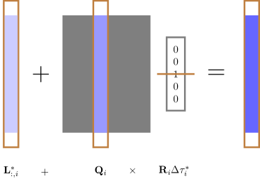
(a)

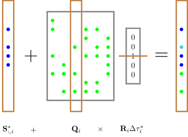
(b)

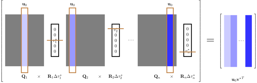
(c)

Figure 2: Illustration of the technical assumptions A.4-A.6: (a) a ${\bf Q}_{i}$ with some columns similar to ${\bf u}^{\ast}$ may induce a vector ${\bf Q}_{i}{\bf R}_{i}\Delta\tau_{i}^{\ast}$ unidentifiable from ${\bf L}_{:,i}^{\ast}$, the $i$-th column of ${\bf L}$; (b) a sparse (coherent) ${\bf Q}_{i}$ may induce a vector ${\bf Q}_{i}{\bf R}_{i}\Delta\tau^{\ast}_{i}$ unidentifiable from ${\bf S}^{\ast}_{:,i}$, the $i$-th column of ${\bf S}^{\ast}$; (c) highly correlated ${\bf Q}_{i}$’s (with a common column ${\bf u}_{0}\in\mathbb{R}^{m}$) may induce a rank-1 matrix $\sum_{i=1}^{n}{\bf J}_{i}\Delta\tau^{\ast}_{i}{\bf e}_{i}^{T}=\sum_{i=1}^{n}{\bf Q}_{i}{\bf R}_{i}\Delta\tau_{i}^{\ast}{\bf e}_{i}^{T}={\bf u}_{0}{{\bf v}^{\ast}}^{T}$ that is unidentifiable from ${\bf L}^{\ast}=\sigma^{\ast}{\bf u}^{\ast}{{\bf v}^{\ast}}^{T}$.

Generally when $\Delta\tau^{\ast}\neq 0$ we have an additional component $\sum_{i=1}^{n}{\bf J}_{i}\Delta\tau_{i}^{\ast}{\bf e}_{i}^{T}$, and in the same spirit we need to ensure it is identifiable from both ${\bf L}^{\ast}$ and ${\bf S}^{\ast}$. Note A.1 does not prevent ${\bf R}_{i}\Delta\tau_{i}^{\ast}$ from moving towards any directions; in particular, it may be aligned with any one of the standard basis vectors in $\mathbb{R}^{d}$. In such a case ${\bf J}_{i}\Delta\tau_{i}^{\ast}$ will be aligned with one of the columns in ${\bf Q}_{i}$, and it turns out either a sparse ${\bf Q}_{i}$ or a ${\bf Q}_{i}$ with some columns similar to ${\bf u}^{\ast}$ can potentially cause identifiability issues with certain columns of ${\bf L}^{\ast}$ or ${\bf S}^{\ast}$ (see Fig. 2a and Fig. 2b for a depiction). To avoid such cases we need two additional assumptions:

1. $\max_{ij}\|{\bf Q}_{j}^{T}{\bf e}_{i}\|_{\ell_{2}}\leq\nu\sqrt{\frac{d}{m}}$ for some $\nu>0$;

2. $\max_{i}\|{\bf Q}_{i}^{T}{\bf u}^{\ast}\|_{\ell_{2}}\leq\kappa\sqrt{\frac{d}{m}}$ for some $\kappa>0$;

here we follow the idea of incoherence in A.4 to measure non-sparsity of ${\bf Q}_{i}$, and in A.5 to measure the dissimilarity between ${\bf Q}_{i}$ and ${\bf u}^{\ast}$. Finally, note that highly-correlated column vectors in different ${\bf Q}_{i}$’s may raise identifiability issues between ${\bf L}^{\ast}$ and $\sum_{i=1}^{n}{\bf J}_{i}\Delta\tau_{i}^{\ast}{\bf e}_{i}^{T}$ (see Fig. 2c for an example); hence we further assume small first principal angles [43] between ${\bf Q}_{i}$’s (on average):

1. $\frac{1}{n-1}\sum_{j\neq i}\|{\bf Q}_{j}^{T}{\bf Q}_{i}\|_{2}\leq\delta$ for some $\delta>0$.

Equipped with assumptions A.1-A.6, we are now ready to state our major theorem as follows:

Theorem 1.

There are positive constants $C_{\delta}$, $C_{q}<1$, $C_{d}=\mathcal{O}(\sqrt{m})$, $C_{\alpha_{1}}=\mathcal{O}\left(d^{-1}\right)$, $C_{\alpha_{2}}=\mathcal{O}\left(d^{-\frac{1}{2}}\right)$ such that, if $\alpha_{1}\leq C_{\alpha_{1}}$, $\alpha_{2}\leq C_{\alpha_{2}}$, $d\leq C_{d}$, $\delta\leq C_{\delta}$, $C_{q}\leq q<1$ then $\forall\beta_{0}\in\left[\frac{\widetilde{\mu}\sigma^{\ast}}{\|{\bf D}_{\tau}\|_{2}},\frac{2\widetilde{\mu}\sigma^{\ast}}{\|{\bf D}_{\tau}\|_{2}}\right]$, $\beta_{1}\in\left[2\widetilde{\mu},2.2\widetilde{\mu}\right]$ where $\widetilde{\mu}=\mu^{2}+\gamma\nu$, each ${\bf S}^{k}(k\geq 0)$ in Algorithm 1  satisfies ${\mathrm{Supp}}({\bf S}^{k})\subset{\mathrm{Supp}}({\bf S}^{\ast})$; furthermore, $\forall\varepsilon>0$ and $K\geq\log_{q}\left(\frac{\varepsilon}{\beta_{0}\|{\bf D}_{\tau}\|_{2}}\right)$, $\|\widehat{{\bf L}}-{\bf L}^{\ast}\|_{F}\leq\varepsilon$, $\|\widehat{{\bf S}}-{\bf S}^{\ast}\|_{\ell_{\infty}}\leq\frac{5\varepsilon}{\sqrt{mn}}$, $\|\widehat{\Delta\tau}-\Delta\tau^{\ast}\|_{F}\leq M\varepsilon$ for some $M>0$.

Proof.

We define ${\bf E}^{k}={\bf S}^{\ast}-{\bf S}^{k}$, ${\bf F}^{k}=\sum_{i=1}^{n}{\bf Q}_{i}{\bf Q}_{i}^{T}({\bf S}^{k}-{\bf S}^{\ast}){\bf e}_{i}{\bf e}_{i}^{T}$, ${\bf G}^{k}=\sum_{i=1}^{n}{\bf Q}_{i}{\bf Q}_{i}^{T}({\bf L}^{k}-{\bf L}^{\ast}){\bf e}_{i}{\bf e}_{i}^{T}$ and ${\bf H}^{k}={\bf F}^{k}+{\bf G}^{k}$. We are going to show the two real sequences $s_{k}:=\|{\bf E}^{k}\|_{\ell_{\infty}}$ and $l_{k}:=\max_{i}\|{\bf G}^{k}{\bf e}_{i}\|_{\ell_{2}}$ decrease exponentially, and this will establish a claim about linear convergence. We proceed by induction. For the basic case $k=0$, $\forall(i,j)\not\in{\mathrm{Supp}}({\bf S}^{\ast})$, ${({\bf S}^{\ast})}_{ij}=0$ and it follows that

$$\left|{({\bf D}_{\tau})}_{ij}\right| \leq\|{\bf L}^{\ast}\|_{\ell_{\infty}}+\left\|\sum_{i=1}^{n}{\bf J}_{i}\Delta\tau^{\ast}{\bf e}_{i}{\bf e}_{i}^{T}\right\|_{\ell_{\infty}}$$

$$\leq\sigma^{\ast}\|{\bf u}^{\ast}\|_{\ell_{\infty}}\|{\bf v}^{\ast}\|_{\ell_{\infty}}+\max_{i,j}\left|{\bf e}_{i}^{T}{\bf Q}_{i}{\bf R}_{i}\Delta\tau^{\ast}{\bf e}_{j}\right|$$

$$\leq\sigma^{\ast}\frac{\mu^{2}}{\sqrt{mn}}+\nu\sqrt{\frac{d}{m}}\frac{\sigma^{\ast}}{\sqrt{nd}}\gamma\leq\zeta_{0},$$

and thus ${\left({\bf S}^{0}\right)}_{ij}=0$ and ${\mathrm{Supp}}\left({\bf S}^{0}\right)\subset{\mathrm{Supp}}\left({\bf S}^{\ast}\right)$. Further, for $d\leq\frac{\sqrt{m}}{16\mu^{2}\nu\kappa}$, $l_{0}=\sigma^{\ast}\max_{i}\left\|{\bf Q}_{i}^{T}{\bf u}^{\ast}\right\|_{\ell_{2}}\left|{({\bf v}^{\ast})}_{i}\right|\leq\frac{1}{16\mu\nu\sqrt{d}}\frac{\sigma^{\ast}}{\sqrt{n}}$ and $s_{0}=\|{\bf E}^{0}\|_{\ell_{\infty}}\leq\zeta^{0}+\|{\bf L}^{\ast}\|_{\ell_{\infty}}+\|\sum_{i=1}^{n}{\bf J}_{i}\Delta\tau^{\ast}{\bf e}_{i}{\bf e}_{i}^{T}\|_{\ell_{\infty}}\leq\frac{3\sigma^{\ast}\widetilde{\mu}}{\sqrt{mn}}$. Assume that $l_{k}\leq\frac{1}{16\mu\nu\sqrt{d}}\frac{\sigma^{\ast}q^{k}}{\sqrt{n}}$, ${\mathrm{Supp}}({\bf S}^{k})\subset{\mathrm{Supp}}({\bf S}^{\ast})$ and $s_{k}\leq\frac{5\widetilde{\mu}\sigma^{\ast}q^{k}}{\sqrt{mn}}$; we can show that $l_{k+1}\leq\frac{1}{16\mu\nu\sqrt{d}}\frac{\sigma^{\ast}q^{k+1}}{\sqrt{n}}$, ${\mathrm{Supp}}({\bf S}^{k+1})\subset{\mathrm{Supp}}({\bf S}^{\ast})$ and $s_{k+1}\leq\frac{5\widetilde{\mu}\sigma^{\ast}q^{k+1}}{\sqrt{mn}}$. We defer this procedure to the supplementary document. For $K\geq\log_{q}\left(\frac{\varepsilon}{\beta_{0}\|{\bf D}_{\tau}\|_{2}}\right)$, and by (40) in the supplementary document, $\|{\bf L}^{K}-{\bf L}^{\ast}\|_{\ell_{\infty}}\leq\frac{\mu^{2}\sigma^{\ast}q^{K}}{\sqrt{mn}}\leq\beta_{0}\frac{\|{\bf D}_{\tau}\|_{2}q^{K}}{\sqrt{mn}}\leq\frac{\varepsilon}{\sqrt{mn}}$ and $\|\widehat{{\bf S}}-{\bf S}^{\ast}\|_{\ell_{\infty}}=\|{\bf S}^{K}-{\bf S}^{\ast}\|_{\ell_{\infty}}\leq 5\beta_{0}\frac{\|{\bf D}_{\tau}\|_{2}q^{K}}{\sqrt{mn}}\leq\frac{5\varepsilon}{\sqrt{mn}}$; thus $\|\widehat{{\bf L}}-{\bf L}^{\ast}\|_{F}=\|{\bf L}^{K}-{\bf L}^{\ast}\|_{F}\leq\sqrt{n}l_{K}\leq\frac{\varepsilon}{16\mu^{3}\nu\sqrt{d}}$ and $\|{\bf S}^{K}-{\bf S}^{\ast}\|_{F}\leq\sqrt{\alpha_{1}mn}s_{K}$, and therefore

$$\|\widehat{\Delta\tau}-\Delta\tau^{\ast}\|_{F} =\|\Delta\tau^{K}-\Delta\tau^{\ast}\|_{F}$$

$$=\sqrt{\sum_{i=1}^{n}\|{\bf J}_{i}^{\dagger}({\bf L}^{K}-{\bf L}^{\ast}+{\bf S}^{K}-{\bf S}^{\ast}){\bf e}_{i}\|_{\ell^{2}}^{2}}$$

$$\leq\left(\max_{1\leq i\leq n}\|{\bf J}_{i}^{\dagger}\|_{2}\right)\left(\frac{1}{16\mu^{3}\nu\sqrt{d}}+5\sqrt{\alpha_{1}}\right)\varepsilon.$$

∎

We only present a sketch of the key arguments above, the detailed proof is available in the supplementary document.

To get a sense for computational complexity, note that step 3 in Algorithm 1 can be done in ${\mathcal{O}}(mn)$ time without invoking full SVD [44]. The approximate complexity for Algorithm 1 is thus ${\mathcal{O}}(mnd^{2}\log\left(\frac{1}{\varepsilon}\right))$ to achieve $\varepsilon$ accuracy.

Remark.

The assumptions stated above are in fact quite reasonable. Assumption A.1 is reasonable as $\Delta\tau$ is expected to be relatively small (note this condition is on $\Delta\tau$ and not $\tau$) by design. Assumptions A.2 and A.3 are widely accepted in the relevant literature [32, 33, 34, 39]. Assumptions A.4 to A.6 serve to avoid identifiability issues. We must emphasize that A.4 — A.6 may not always hold for a ${\mathbf{D}}_{\tau}$ formed from practical datasets. Note however, that these conditions when fully satisfied provide rather strong exact recovery guarantees as confirmed via Theorem 7 (or perfect alignment). In practice, even with departures from some of these conditions, enforcing a rank-1 constraint is highly meritorious and leads to improved performance. Experimental studies that corroborate this follow in Section IV-C.

II-D Relationship to Traditional Pixel-Based Methods

There is a large variety of pixel-based methods in the image alignment literature as [4, 5, 6, 7]. Invariably, they work on aligning image pairs by solving:

$$\min_{\tau,{\mathcal{P}}}\rho(I_{2}\circ\tau,{\mathcal{P}}(I_{1}))$$ (10)

where $I_{1}$, $I_{2}$ are given image pairs to be aligned, and $\tau$, ${\mathcal{P}}$ are the geometric and photometric transformations, respectively. The real-valued function $\rho$ obeys $\rho(I_{1},I_{2})\geq 0$ and equals $0$ if and only if $I_{1}=I_{2}$. For instance, the method in [4] corresponds to $\rho(I_{1},I_{2})=\|I_{1}-I_{2}\|^{2}_{2}$ and ${\mathcal{P}}(I)=I$, whereas in [5] an affine model on $I$ is used. Regularizers may also be added. For instance, the method in [7] encourages smoothness of the warp and shrinkage at the self-occlusion boundary. To handle occlusions, error functions such as the Huber loss function [45] may be used.

As a clear benefit, our method can of course work on aligning a batch of images. We can draw an analogy between traditional pixel-based methods and ours when $n=2$. We let ${\bf D}=[{\mathrm{vec}}(I_{2}),{\mathrm{vec}}(I_{1})]$. Through eliminating ${\bf S}$, we may rewrite (4) as

$$\min_{{\bf L},\tau}\|{\bf D}\circ\tau-{\bf L}\|_{\ell^{1}},\quad\text{ subject to }\mathrm{rank}({\bf L})=1,$$ (11)

Note that $\mathrm{rank}({\bf L})=1$ if and only if its two columns $L_{1},L_{2}\in\mathbb{R}^{m}$ are linearly dependent. In most cases of interest, ${\bf L}=0$ will not be the minimizer to (4), and without loss of generality we can write $L_{1}=gL_{2}$ for some constant $g>0$. Therefore, we may drop the rank-1 constraint and rewrite (11) as

$$\min_{g,L_{2},\tau}\|I_{2}\circ\tau-gL_{2}\|_{\ell^{1}}+\|I_{1}-L_{2}\|_{\ell^{1}}.$$ (12)

Thus our method acts like “mean absolute deviation” (around the median) of $I_{2}\circ\tau$ and $I_{1}$, with $g$ accounting for the photometric differences. When there are multiple images ($n\geq 3$), pairwise registration may be suboptimal [1]. It is less obvious to extend (10) to such cases than (11). From this perspective, our method provides a principled approach of jointly aligning multiple images and accounts for photometric differences and occlusions simultaneously.

III Bundle Robust Alignment for Practical Image Stitching

The flowchart of our panoramic image composition scheme is illustrated in Fig. 3.

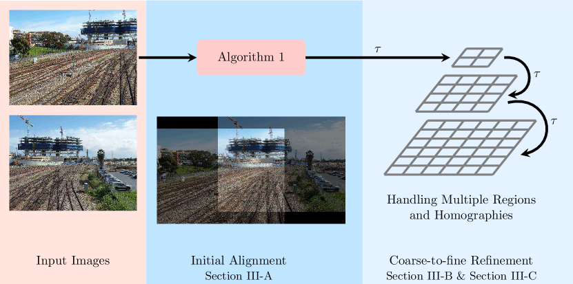
Figure 3: Flowchart of our panoramic alignment for stitching pipeline. See Section III-A to III-C for details.

III-A Estimating Initial Transformation Parameters

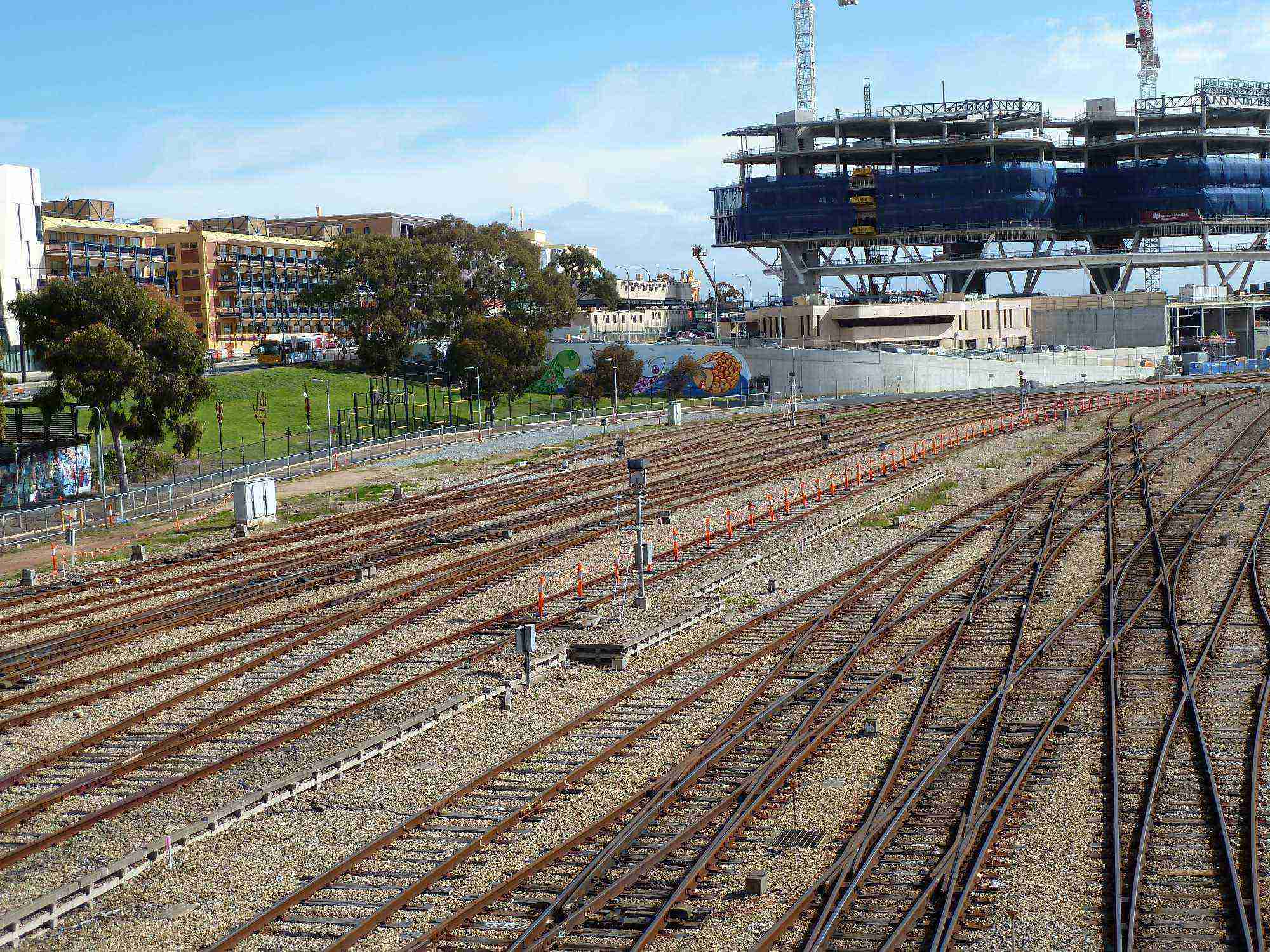
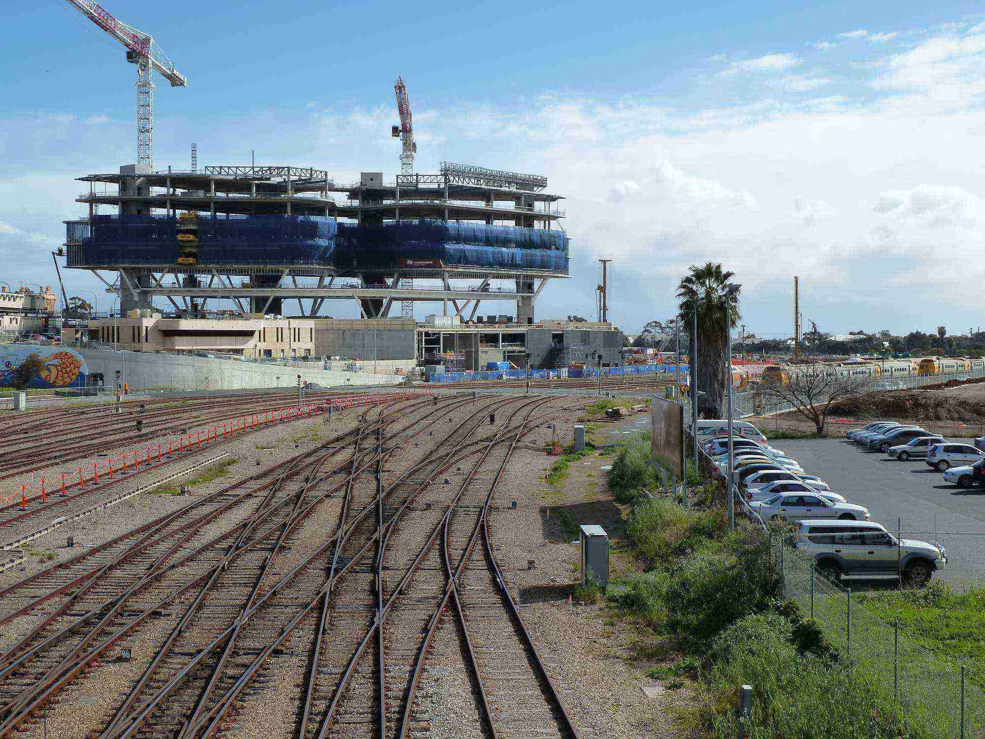
(a) Input

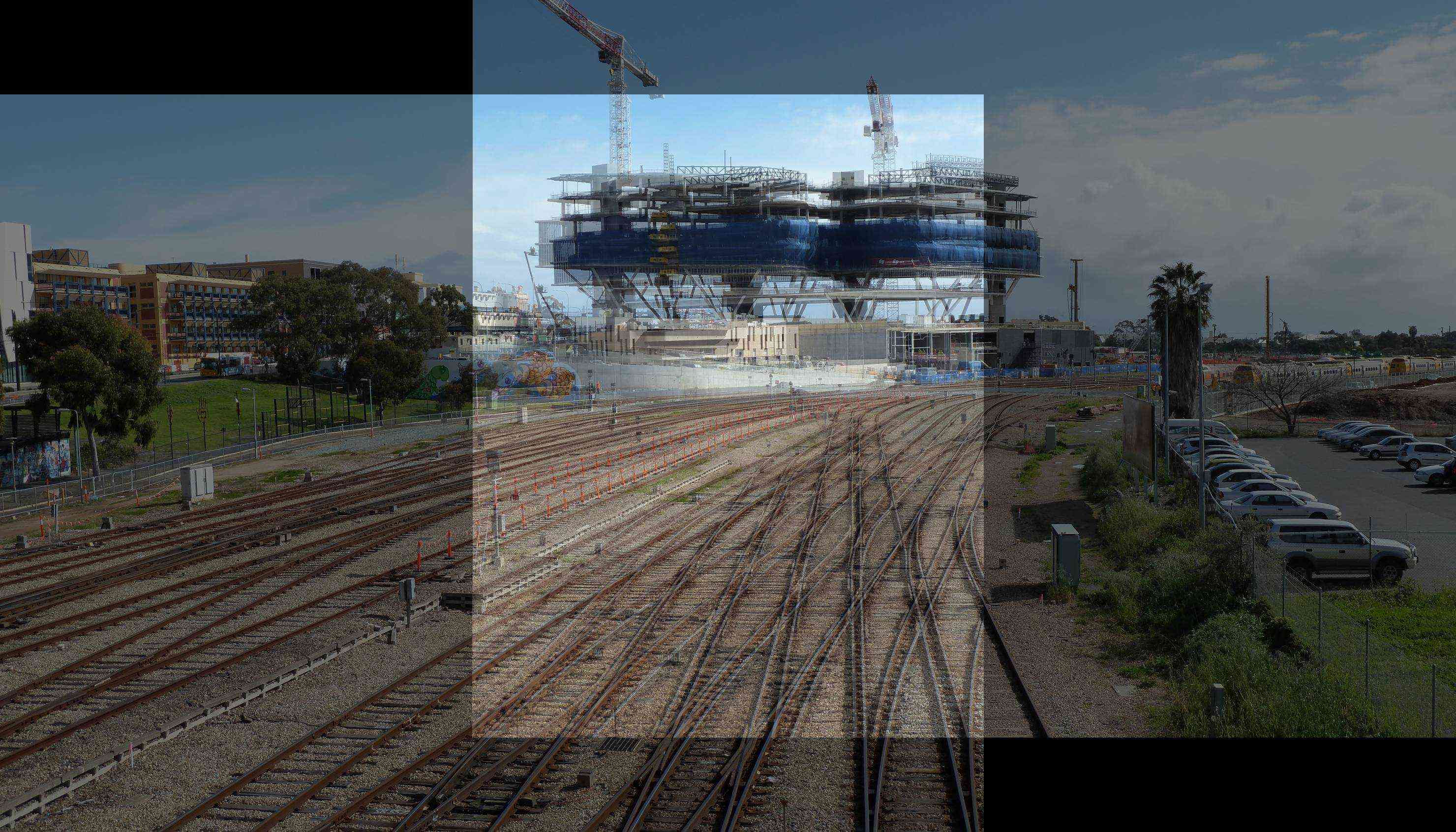
(b) Initially Aligned

Figure 4: Initially aligned and overlayed images on the railtracks [12] dataset, using the method in Section III-A. Rescaled for better display.

The iterative linearization scheme discussed in Section II-A becomes invalid when $\tau$ is large. To mitigate this, we adopt a coarse-to-fine pyramidal implementation: we decompose the images into Gaussian pyramids, and progressively refine $\tau$ at each scale. In image stitching, the displacements between images are often large, and we still need to properly initialize $\tau$ at the beginning of the coarsest scale. One way of accomplishing this is by traditional pixel based methods but they cannot handle large displacements. Therefore, in the following, we develop a probabilistic approach.

For multiple images, we estimate the parameters between consecutive pairs of images, and then chain them together. For each pair of images, we extract their corresponding SIFT images [2] $s_{1}$ and $s_{2}$ where $s_{i}(i=1,2)$ comprises a 128-dimensional SIFT feature vector per pixel. Let $\tau_{12}$ be the transformation (homography) parameters from $s_{2}$ to $s_{1}$. Our idea is to estimate $\tau_{12}$ from dense correspondences (motion field) between $s_{1}$ and $s_{2}$. We leverage a robust error function as the difference measure between $s_{1}$ and $s_{2}$ to address large displacements and significant occlusions. We also enforce spatial contiguity on the motion field to enhance robustness.

Let ${\bf s}=\{s_{1},s_{2}\}$. For tractability of minimization, we model the relationship between ${\bf s}$ and $\tau_{12}$ using Hidden Markov Random Field (HMRF): we view ${\bf s}$ as observed variables, and the motion vector ${\bf w}({\bf p})=(u({\bf p}),v({\bf p}))$ at every pixel ${\bf p}$ as latent variables. Here $u({\bf p}),v({\bf p})$ take integer values between $-L$ and $L$ for a given integer $L$ that serves as an upper bound on the pixel displacements. Let ${\bf w}={\{{\bf w}({\bf p})\}}_{\bf p}$. We then set up the following probabilistic models:

$$p({\bf s}|{\bf w})\propto\exp\biggl{\{}- \sum_{{\bf p}}\min(\|s_{1}({\bf p})-s_{2}({\bf p}+{\bf w}({\bf p}))\|_{\ell_{1}},\kappa)\biggr{\}},$$ (13)

$$p({\bf w}|\tau_{12})\propto\exp\biggl{\{}- \eta\sum_{{\bf p}}\|{\bf w}({\bf p})-t({\bf p};\tau_{12})\|_{\ell_{1}}$$ (14)

$$- \alpha\sum_{({\bf p},{\bf q})\in\mathcal{N}}\|{\bf w}({\bf p})-{\bf w}({\bf q})\|_{\ell_{2}}^{2}\biggr{\}},$$ (15)

where $\kappa,\eta,\alpha$ are positive constants, and $\mathcal{N}$ comprises all pairs of 4-connected neighboring pixels. (13) enforces robust feature matching similar to [2]; (14) encourages small deviations of ${\bf w}({\bf p})$ from $t({\bf p};\tau_{12})$, the coordinate of ${\bf p}$ under the transformation represented by $\tau_{12}$, while (15) encourages small differences of ${\bf w}$ between adjacent pixels ${\bf p}$, ${\bf q}$. We estimate $\tau_{12}$ following the maximum likelihood estimation principle:

$$\widehat{\tau_{12}}\leftarrow\arg\max_{\tau_{12}}\sum_{\bf w}p({\bf s}|{\bf w})p({\bf w}|\tau_{12}).$$ (16)

A standard approach to solving (16) is the expectation-maximization (EM) algorithm [46], as listed in Algorithm 2, where we let $t({\bf p};\tau_{12})=(t_{u}({\bf p};\tau_{12}),t_{v}({\bf p};\tau_{12}))$. To monitor the convergence behavior, we define $d_{h,w}(\tau_{1},\tau_{2})$ to measure the difference between transformation parameters $\tau_{1}$ and $\tau_{2}$:

$$d_{h,w}(\tau_{1},\tau_{2})=\frac{1}{hw}\sum_{x=1}^{w}\sum_{y=1}^{h}\left\|t((x,y);\tau_{1})-t((x,y);\tau_{2})\right\|_{\ell_{2}}^{2},$$ (17)

i.e., it measures the mean squared error between transformed coordinates $t((x,y);\tau_{1})$ and $t((x,y);\tau_{2})$ by applying $t(\cdot;\tau_{1})$ and $t(\cdot;\tau_{2})$ to an $h\times w$ image. Fig. 4 shows an example of the initialization. The images are rescaled to the original resolution for display purposes. After running Algorithm 2, the images are coarsely aligned but Algorithm 3 in Section III-B (which employ the rank-1 constraint) is required for precise alignment.

Algorithm 2 Initial Transformation Parameter Estimation

0:  SIFT images $s_{1},s_{2}\in\mathbb{R}^{w_{2}\times h_{2}\times 128}$, $\epsilon>0,L\in\mathbb{N}$.

1:  Initialize $\tau_{12}^{0}$ to identity transformation, $k\leftarrow 0$.

2:  repeat

3:     Use belief propagation [47] to compute probabilities $\omega_{{\bf p},l}^{u}\leftarrow p(u({\bf p})=l|{\bf s},\tau_{12}^{k})$, $\omega_{{\bf p},l}^{v}\leftarrow p(v({\bf p})=l|{\bf s},\tau_{12}^{k}),\forall$ pixel ${\bf p},l=-L,-L+1,\dots,L$.

4:     $k\leftarrow k+1$.

5:     $\tau_{12}^{k}\leftarrow\arg\min_{\tau_{12}}\sum_{{\bf p}}\sum_{l=-L}^{L}|t_{u}({\bf p};\tau_{12})-l|\omega^{u}_{{\bf p},l}+|t_{v}({\bf p};\tau_{12})-l|\omega_{{\bf p},l}^{v}$.

6:  until $d_{h_{2},w_{2}}(\tau_{12}^{k},\tau_{12}^{k-1})<\epsilon$

6:  estimated transformation parameters $\widehat{\tau_{12}}$.

III-B Handling Multiple Overlapping Regions

When there are multiple input images they usually overlap across multiple regions. We have experimentally observed that simply zero-padding the warped images to the size of canvas often causes divergence; on the other hand, the naive way of applying pairwise alignment consecutively is suboptimal since the alignment errors may propagate and accumulate [1]. Therefore, it is essential to develop a method to account for the complicated overlapping relationships simultaneously.

The basic idea is to apply the rank-1 and sparse decomposition discussed in Section II on every overlapping region. A visualization of the model is in Fig. 5. We again let $m$ be the number of pixels on canvas and $n$ be the number of images. The $m\times n$ matrix thus formed is called the canvas matrix. We will consistently use $r$ as region index and $i$ as image index. $\sum_{r}$ and $\sum_{i}$ means summing over each region and each image, respectively. Assuming predetermined regions, we reformulate Equation (4) as

$$\min_{{\{{\bf L}_{r}\}}_{r},{\{{\bf S}_{r}\}}_{r},\tau}\quad \sum_{r}\left\|{\bf S}_{r}\right\|_{\ell_{1}}$$ (18)

$$\text{subject to}\quad{\mathcal{R}}_{r}({\bf D}\circ\tau) ={\bf L}_{r}+{\bf S}_{r},\quad\forall r,$$

$$\mathrm{rank}({\bf L}_{r}) =1,\qquad\forall r,$$

where ${\mathcal{R}}_{r}:\mathbb{R}^{m\times n}\rightarrow\mathbb{R}^{m_{r}\times n_{r}}$ is the operator that extracts the portion of ${\bf D}\circ\tau$ belonging to the $r$-th region and ${\bf L}_{r}$, ${\bf S}_{r}\in\mathbb{R}^{m_{r}\times n_{r}}$ are the corresponding rank-1 and sparse components. The linearized problem is

$$\min_{{\{{\bf L}_{r}\}}_{r},{\{{\bf S}_{r}\}}_{r},\Delta\tau}\quad\sum_{r}\left\|{\bf S}_{r}\right\|_{\ell_{1}}$$

$$\text{subject to}\quad{\bf D}_{r}+\sum_{i\in{\mathcal{I}}_{r}}{\bf J}_{r,i}\Delta\tau_{i}{\bf e}_{f_{r}^{i}}^{T} ={\bf L}_{r}+{\bf S}_{r},\quad\forall r,$$

$$\mathrm{rank}({\bf L}_{r}) =1,\qquad\forall r,$$ (19)

where we write ${\mathcal{R}}_{r}({\bf D}\circ\tau)$ as ${\bf D}_{r}$ for brevity; ${\bf J}_{r,i}\in\mathbb{R}^{m_{r}\times d}$ is the Jacobian of the $i$-th image restricted to the $r$-th region. We let ${\mathcal{I}}_{r}$ be the indices of images contributing to the $r$-th overlapping regions, $\bar{{\mathcal{I}}}_{i}$ be the indices of regions in the $i$-th image, and $f_{r}^{i}$ be the column index of the $i$-th image in ${\bf D}_{r}$. Algorithm 3 is used to solve (19), and the accompanying theoretical analysis is included in the supplementary document.

Figure 5: The overlapping region model and relevant notations: images on canvas may overlap in different regions, according to which we may determine the data matrices ${\bf D}_{\mathit{1}}$,${\bf D}_{\mathit{2}}$ and ${\bf D}_{\mathit{3}}$. Here ${\mathcal{I}}_{\mathit{1}}=\{1,2\}$, ${\mathcal{I}}_{\mathit{2}}=\{1,2,3\}$; $\bar{{\mathcal{I}}}_{1}=\{\mathit{1},\mathit{2}\}$,$\bar{{\mathcal{I}}}_{2}=\{\mathit{1},\mathit{2},\mathit{3}\}$; $f_{\mathit{3}}^{2}=1$, $f_{\mathit{3}}^{3}=2$, etc.

In practice, we determine the regions approximately by updating them at each linearization step before solving (19). Specifically, we warp the images using the currently estimated $\tau$ and repeatedly scope out the overlapping regions. Each time we pick the region with the highest number of contributing images until no overlaps remain.

Algorithm 3 Alternating Minimization for Solving (19)

0:  ${\{{\bf D}_{r}\in\mathbb{R}^{m_{r}\times n_{r}}\}}_{r}$, ${\{{\bf J}_{r,i}\in\mathbb{R}^{m_{r}\times d}\}}_{r,i}$,$\beta_{0}$,$\beta_{1}$,$q>0$.

1:  for all $r$ do

2:     ${\bf S}_{r}^{0}\leftarrow{\mathcal{S}}_{\zeta_{r}^{0}}({\bf D}_{r})$ where $\zeta_{r}^{0}=\beta_{0}\frac{\|{\bf D}_{r}\|_{2}}{\sqrt{m_{r}n_{r}}}$.

3:  end for

4:  $\Delta\tau^{0}\leftarrow\sum_{i}\sum_{r\in\bar{{\mathcal{I}}}_{i}}{\left(\sum_{l\in\bar{{\mathcal{I}}}_{i}}\frac{{\bf J}_{l,i}^{T}{\bf J}_{l,i}}{\zeta_{l}^{0}}\right)}^{\dagger}\frac{{\bf J}_{r,i}^{T}({\bf S}_{r}^{0}-{\bf D}_{r}){\bf e}_{f_{r}^{i}}{\bf e}_{i}^{T}}{\zeta_{r}^{0}}$.

5:  for $k=1,2,\dots,K$ do

6:     for all $r$ do

7:        ${\bf L}_{r}^{k}\leftarrow{\mathcal{T}}_{1}\left\{{\bf D}_{r}+\sum_{i\in\mathcal{I}_{r}}{\bf J}_{r,i}\Delta\tau_{i}^{k-1}{\bf e}_{f_{r}^{i}}^{T}-{\bf S}_{r}^{k-1}\right\}$,

8:        $\zeta_{r}^{k}\leftarrow\beta_{1}\frac{q^{k}}{\sqrt{m_{r}n_{r}}}\|{\bf L}_{r}^{k}\|_{2}$,

9:        ${\bf S}_{r}^{k}\leftarrow{\mathcal{S}}_{\zeta_{r}^{k}}\left\{{\bf D}_{r}+\sum_{i\in\mathcal{I}_{r}}{\bf J}_{r,i}\Delta\tau_{i}^{k-1}{\bf e}_{f_{r}^{i}}^{T}-{\bf L}_{r}^{k}\right\}$.

10:     end for

11:     $\Delta\tau^{k}\leftarrow\sum_{i,r\in\bar{{\mathcal{I}}}_{i}}\!\!{\left(\sum_{l\in\bar{{\mathcal{I}}}_{i}}\!\!\frac{{\bf J}_{l,i}^{T}{\bf J}_{l,i}}{\zeta_{l}^{k}}\right)}^{\dagger}\!\frac{{\bf J}_{r,i}^{T}({\bf L}_{r}^{k}+{\bf S}_{r}^{k}-{\bf D}_{r}){\bf e}_{f_{r}^{i}}{\bf e}_{i}^{T}}{\zeta_{r}^{k}}$.

12:  end for

12:  $\widehat{{\bf L}_{r}}\leftarrow{\bf L}_{r}^{K}$, $\widehat{{\bf S}_{r}}={\bf S}_{r}^{K}$, $\widehat{\Delta\tau}=\Delta\tau^{K}$.

III-C Extension to Multiple Homographies

Recent studies [13, 12] have revealed that the classic single homography model is inadequate to represent camera motions accurately for casually taken photos. Fig. 6 illustrates one such example. To handle such cases, we need to extend our method to incorporate more general motion models.

​

(a) Input

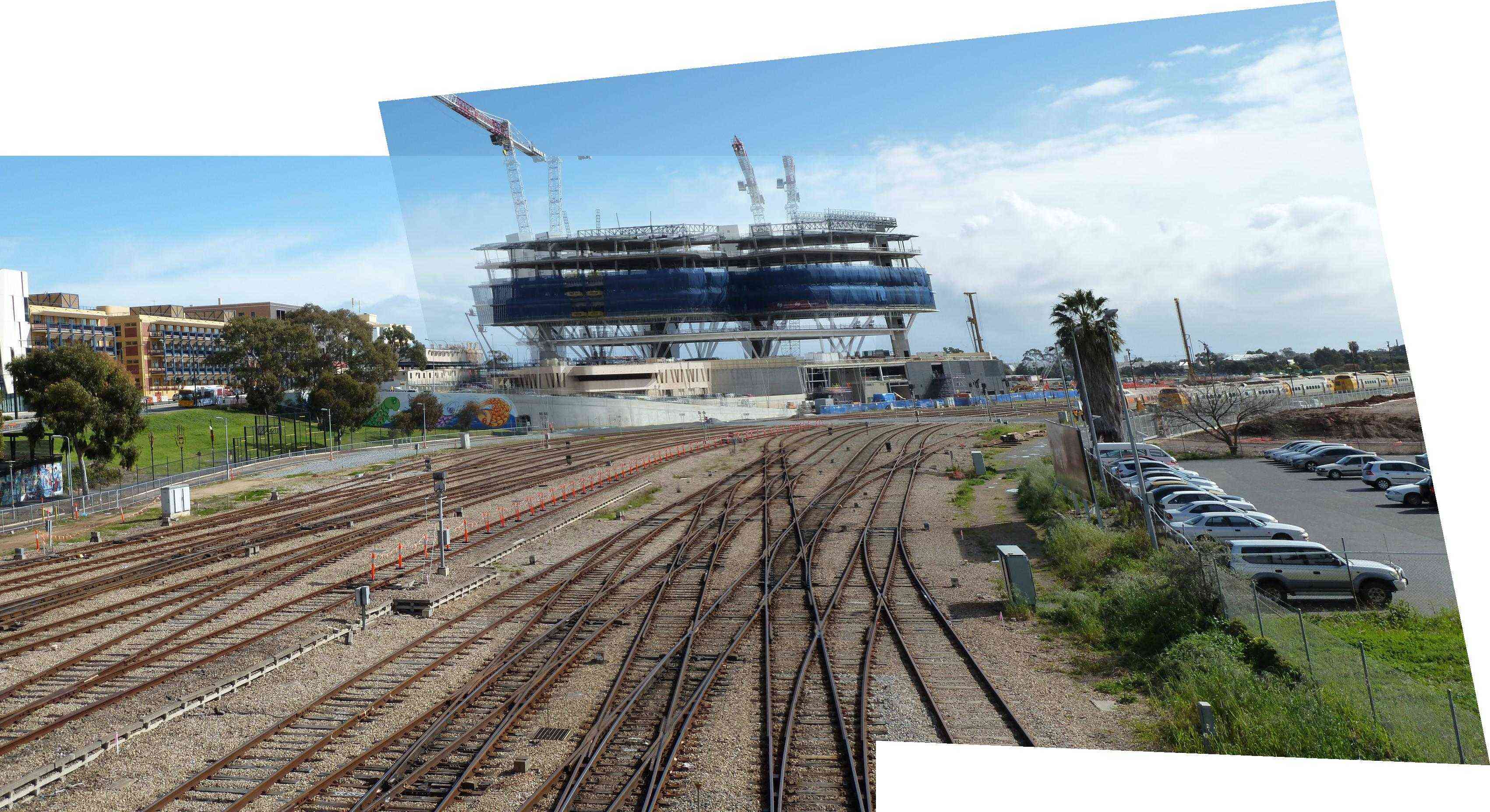
(b) Overlayed

Figure 6: A failure case of single homography in modeling camera motion: the homography estimated using the ground plane induces apparent misalignments of the building.

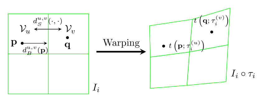
Figure 7: Illustration of the multiple homography model and relevant notations: we divide each image $I_{i}$ into cells, and associate each cell with its own set of homography parameters. We further encourage smoothness of the homographies in neighboring cells $u$ and $v$.

While our approach may be combined with generic motion models, developing a dedicated flexible model is outside the scope of this work. Moreover, we would like to ensure consistency in experimental comparisons. To this end, we integrate the model in [12] into our approach. Specifically, we partition each image (indexed by $i$) into $C_{1}\times C_{2}$ cells, and warp each cell (indexed by $u$) using an individual set of homography parameters $\tau_{i}^{(u)}$. We stack $\tau_{i}^{(u)}$s together as $\tau_{i}={\left(\tau_{i}^{(u)}\right)}_{u}$ and define $I_{i}\circ\tau_{i}$ as the image warped cell by cell. A visual depiction of this model is in Fig. 7.

To avoid tearing the objects and maintain stability in extrapolation along non-overlapping regions, it is necessary to enforce smoothness of the underlying geometric transformation. We thus introduce a smoothness term over $\tau$ and modify problem (18) as:

$$\min_{{\{{\bf L}_{r}\}}_{r},{\{{\bf S}_{r}\}}_{r},\tau}\quad\sum_{r}\left\|{\bf S}_{r}\right\|_{\ell_{1}} +\frac{\lambda}{2}\sum_{i=1}^{n}\sum_{(u,v)\in{\mathcal{E}}_{i}}d^{u,v}_{S}\left(\tau_{i}^{(u)},\tau_{i}^{(v)}\right)$$

$$\text{subject to}\quad{\mathcal{R}}_{r}({\bf D}\circ\tau) ={\bf L}_{r}+{\bf S}_{r},\quad\forall r$$

$$\mathrm{rank}({\bf L}_{r}) =1,\qquad\forall r,$$ (20)

where $\lambda>0$ is a constant parameter that controls the strength of smoothness, ${\mathcal{E}}_{i}$ comprises pairs of adjacent cells in the $i$-th image and $d^{u,v}_{S}\left(\tau_{i}^{(u)},\tau_{i}^{(v)}\right)$ promotes smoothness between $\tau_{i}^{(u)}$ and $\tau_{i}^{(v)}$, defined as the following:

$$\sum_{{\bf p}\in{{\mathcal{V}}_{u}\cup{\mathcal{V}}_{v}}}\exp{\left\{-\frac{{d_{B}^{u,v}({\bf p})}^{2}}{\sigma^{2}}\right\}}\left\|t\left({\bf p};\tau_{i}^{(u)}\right)-t\left({\bf p};\tau_{i}^{(v)}\right)\right\|_{\ell_{2}}^{2},$$ (21)

where $\sigma>0$ is a constant parameter, ${\mathcal{V}}_{u}$ and ${\mathcal{V}}_{v}$ collect pixels in cell $u$ and $v$, respectively, and $d_{B}^{u,v}({\bf p})$ is the Euclidean distance from ${\bf p}$ to the common boundary of cell $u$ and $v$. The reasoning behind $d^{u,v}_{S}(\cdot,\cdot)$ is to encourage neighboring homographies to be consistent on pixels close to the cell boundaries and thus prevent discontinuities along those boundaries.

To solve (20), we can adopt the same iterative linearization scheme as in Section II-B; in addition to $I_{i}\circ\tau_{i}$, we linearize each $t\left({\bf p};\tau^{(u)}_{i}\right)$ in (21) with respect to $\tau^{(u)}_{i}$ as: $t\left({\bf p};\tau_{i}^{(u)}+\Delta\tau_{i}^{(u)}\right)\approx t\left({\bf p};\tau_{i}^{(u)}\right)+{\bf J}_{i}^{(u)}\Delta\tau_{i}^{(u)}$ where ${\bf J}_{i}^{(u)}=\left.\frac{\partial t({\bf p};\xi)}{\partial\xi}\right|_{\xi=\tau_{i}^{(u)}}$. The optimization algorithm for solving the linearized subproblems of (20) resembles Algorithm 3, except that in Step 4 and 11 the following formula should be used instead (for $k\geq 0$):

$$\Delta\tau^{k}\leftarrow\sum_{i=1}^{n}\!\!{\left(\sum_{l\in\bar{{\mathcal{I}}}_{i}}\!\!\frac{{\bf J}_{l,i}^{T}{\bf J}_{l,i}}{\zeta_{l}^{k}}+\lambda\bm{\Gamma}_{i}\right)}^{\dagger}\!\left({\bf r}^{k}_{i}+\lambda{\bf t}_{i}\right){\bf e}_{i}^{T}$$

where ${\bf r}^{k}_{i}=\sum_{r\in\bar{{\mathcal{I}}}_{i}}\frac{{\bf J}_{r,i}^{T}}{\zeta_{r}^{k}}\left({\bf L}_{r}^{k}+{\bf S}_{r}^{k}-{\bf D}_{r}\right){\bf e}_{f_{r}^{i}}$ and we define ${\bf L}_{r}^{0}=0$. $\bm{\Gamma}_{i}$, ${\bf t}_{i}$ are obtained by organizing the following linear system into the form $\bm{\Gamma}_{i}\Delta\tau_{i}={\bf t}_{i}$:

$$\sum_{v\in{\mathcal{N}}_{u}}\sum_{{\bf p}\in{\mathcal{V}}_{u}\cup{\mathcal{V}}_{v}}w_{{\bf p}}^{u,v}{{\bf J}_{i}^{(u)}}^{T}\left[{\bf J}_{i}^{(u)}\Delta\tau_{i}^{(u)}-{\bf J}_{i}^{(v)}\Delta\tau_{i}^{(v)}\right]$$ (22)

$$= \sum_{v\in{\mathcal{N}}_{u}}\sum_{{\bf p}\in{\mathcal{V}}_{u}\cup{\mathcal{V}}_{v}}w_{{\bf p}}^{u,v}{{\bf J}_{i}^{(u)}}^{T}\left[t\left({\bf p};\tau_{i}^{(v)}\right)-t\left({\bf p};\tau_{i}^{(u)}\right)\right],\,\forall u,$$

where $w_{{\bf p}}^{u,v}=\exp{\left\{-\frac{{d^{u,v}_{B}({\bf p})}^{2}}{\sigma^{2}}\right\}}$ and ${\mathcal{N}}_{u}$ comprises cells adjacent to $u$. After aligning all the images, we employ seam-cutting [48] and gradient-domain blending [49] to stitch them.

IV Experimental Results

IV-A Experimental Settings

To evaluate the influence of different parameter choices on alignment performance, we collect a validation set comprising $5$ sets of images to be aligned. The images are taken from Adobe Panorama Dataset [50]. To quantitatively assess the performance of BRAS, we introduce truncated $\ell_{2}$-norm $d_{t}$ between images $I_{1}$ and $I_{2}$:

$$d_{t}(I_{1},I_{2})=\sqrt{\frac{1}{m}\sum_{i=1}^{m}\min(\|I_{1}({\bf p}_{i})-I_{2}({\bf p}_{i})\|^{2}_{\ell_{2}},t^{2})},$$

where $t$ is a positive constant fixed to $25$ intensity values in all the experiments, $I_{1}({\bf p}_{i})$ and $I_{2}({\bf p}_{i})$ are the values of the $i$-th pixel in the overlapping region (comprising $m$ pixels) from image $I_{1}$ and $I_{2}$, respectively. This quantity serves as a robust measure of alignment accuracy [51], and smaller value generally indicates higher alignment accuracy. For more than two images, errors are computed pairwise and then accumulated. The average values of this metric under various parameter settings are summarized in Table I.

It can be clearly observed that the performance of BRAS is robust to small perturbations of its parameter values. Therefore, unless otherwise stated, we set $\beta_{0}=\beta_{1}=1$, $q=0.7$ in Algorithm 3. In (14) $\eta$ takes either $10^{-3}$ or $10^{-4}$ while in (15) $\alpha$ is chosen as either $1$ or $10$. The number of cells (as described in III-C) is fixed to $C_{1}=C_{2}=16$, and we reduce it by half when moving to a higher pyramid level. In (20) we choose $\lambda=N_{p}$ or $\lambda=10N_{p}$ where $N_{p}$ is the number of pixels in each cell while in (21) we let $\sigma=0.2$. We choose $\epsilon=10^{-3}$ in Algorithm 2, and $\epsilon=10^{-5}$ in Algorithm 3. We employ normalized coordinates as suggested in [52] for better conditioning of the linear system in Equation (22).

TABLE I: Effects of parameter variations on alignment accuracy (measured in truncated $\ell^{2}$ norm).

$\beta_{0},\beta_{1}$	$q$	$\eta$	$\alpha$	$\sigma$	$C_{1},C_{2}$	Truncated $\ell^{2}$ norm
$1$	$0.5$	$10^{-3}$	$10$	$0.2$	$16$	$7.55$
$1$	$0.7$	$10^{-3}$	$10$	$0.2$	$16$	$7.51$
$1.5$	$0.5$	$10^{-3}$	$10$	$0.2$	$16$	$7.50$
$1$	$0.5$	$10^{-4}$	$10$	$0.2$	$16$	$7.55$
$1$	$0.5$	$10^{-3}$	$1$	$0.2$	$16$	$7.55$
$1$	$0.5$	$10^{-3}$	$10$	$0.3$	$16$	$7.59$
$1$	$0.5$	$10^{-3}$	$10$	$0.2$	$8$	$7.58$

For results generated with competing state of the art methods, we either use publicly available code with instructions made available by the authors of the work or contacted the authors directly for generation of results. For fairness in comparison, we consistently apply the same stitching method described in Section III-C across all methods.

IV-B Validation on Random Simulations

(a) Convergence speed

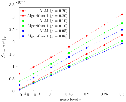
(b) Stability under noise

Figure 8: Performance evaluation under different occlusion levels $\rho$. LABEL:sub@fig:convergence The convergence rate of Algorithm 1 is linear and it achieves lower final errors than ALM; LABEL:sub@fig:noise Algorithm 1 degrades less with increasing noise levels compared with ALM.

We perform random simulations to quantitatively study the performance of Algorithm 1 and verify the assertions of Theorem 7. We let $m=500$, $n=10$, and generate ${\bf D}$ according to formula (9). In accordance with [40], we generate ${\bf L}^{\ast}={\bf u}^{\ast}{{\bf v}^{\ast}}^{T}$ with ${\bf u}^{\ast}\sim{\mathcal{N}}\left(0,\frac{1}{m}{\bf I}_{m}\right)$, ${\bf v}^{\ast}\sim{\mathcal{N}}\left(0,\frac{1}{n}{\bf I}_{n}\right)$ where ${\bf I}_{m}$ is the $m\times m$ identity matrix. The entries of ${\bf S}^{\ast}$ take $-1$ and $1$ independently and equally likely, while ${\mathrm{Supp}}({\bf S}^{\ast})$ is a randomly sampled subset of $\{1,\dots,m\}\times\{1,\dots,n\}$ with cardinality $\rho mn$, $\rho\in(0,1)$. ${\bf J}_{i}\sim{\mathcal{N}}\left(0,\frac{d}{m}{\bf I}_{md}\right)$ and ${\bf R}_{i}\Delta\tau_{i}^{\ast}\sim{\mathcal{N}}\left(0,\frac{\|{\bf L}^{\ast}\|_{2}}{nd}{\bf I}_{d}\right)$. For comparison, we include Algorithm 2 in [3], where an Augmented Lagrange Multiplier (ALM) method was proposed to solve the convex surrogate of (5). We vary $\rho$ to study the influence of different amount of occlusions. We set $q=0.75,0.85,0.95$ in Algorithm 1 when $\rho=0.05,0.1,0.2$, respectively. We execute both algorithms for $50$ iterations and plot their convergence curves in Fig. 8a. Both algorithms progress slower under larger $\rho$, as larger occlusions are generally more difficult to handle. The errors $\|\Delta\tau^{k}-\Delta\tau^{\ast}\|_{F}$ for Algorithm 1 decay exponentially at rate $q$, in agreement with Theorem 7. ALM progresses aggressively up to $20$ iterations, but stays at certain error levels. In contrast, Algorithm 1 steadily progresses towards smaller errors.

In practice, it is often the case that ${\bf D}$ is affected by random noise [53]; in particular, some errors may be introduced in the linearization (5). We study their effects by adding an noise matrix ${\bf N}$ to ${\bf D}$, where ${\bf N}_{ij}\sim{\mathcal{N}}(0,\frac{1}{mn})$. In all cases we set $q=0.95$ in Algorithm 1, and run both algorithms for $100$ iterations for fairness. We measure the errors in their outputs $\widehat{\Delta\tau}$ under varying levels of noise, i.e., different $\sigma$, and different occlusion levels $\rho$. The results are summarized in Fig. 8b. Similar to Fig. 8a, increasing $\rho$ leads to increases in errors in both algorithms. Clearly, Algorithm 1 exhibits smaller errors than ALM in every cases, indicating its higher stability under different amount of noise. Indeed, as we observed in our experiments on real data, our method can tolerate larger deviations of $\tau$ than [3].

IV-C Effectiveness of the Rank-1 Constraint

To further verify the effectiveness of the exact rank-1 constraint as opposed to the conventional convex relaxation approaches, we compare with RASL [3] over the temple dataset [13] under the same settings except that the rank-1 constraint is replaced by the convex relaxation. The results are in Fig. 9. It may be inferred from Fig. 9 that BRAS generates much better alignment. An additional visual comparison is shown in Fig. 20 in the supplementary document.

(a) RASL [3]

(b) BRAS

Figure 9: The effectiveness of the rank-1 constraint: comparison on the temple dataset [13] between RASL and BRAS. The aligned images are overlayed to show the misaligned regions, which are highlighted in red circles. BRAS aligns the images significantly better, as can be seen by the reduction in ghosting artifacts.

To quantitatively characterize the performance limits of RASL and BRAS, we perform a synthetic experimental comparison. In the same spirit as [3], different magnitudes of misalignments (translations in $x$ direction) and different amount of occlusions are studied. Occlusions are simulated by zeroing out pixels at random locations. We consider an alignment successful if for a given translation $t(\cdot;\tau^{\ast})$, the final solution $\widehat{\tau}$ satisfies $d_{h,w}(\tau^{\ast},\widehat{\tau})<1$ pixel spacing for $d_{h,w}(\tau_{1},\tau_{2})$ defined in (17). We test over $10$ commonly used image sets, and randomly select one image from each image set. We count the number of successes and divide it by $10$. The results are summarized in Fig. 10, which confirms that BRAS has much higher tolerance against large translations and occlusions.

(a) RASL [3]

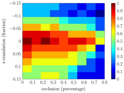
(b) BRAS

Figure 10: Fractions of successful alignments are plotted for RASL and BRAS versus different translations and occlusions. The translations are in percentage of the corresponding image dimensions, while the occlusions are in fractions of the number of pixels.

IV-D Alignment in Challenging Scenarios

For various reasons, images difficult to align may be produced in real world photography. However, for practical purposes such as object recognition, it may be desirable to find a sensible alignment even in such scenarios. We will analyze two typical examples, and assess the performance of BRAS in terms of alignment accuracy. For comparisons, we also evaluate a typical feature-based method with SIFT as descriptors. This method is widely used in panorama software nowadays [9, 54]. In all the cases we adhere to the classic single homography model to rule out the influence of different motion models.

(a)

(b)

(c)

Figure 11: Alignment results under appearance changes: LABEL:sub@fig:christSIFT appearance changes may mislead feature matching, and LABEL:sub@fig:christRANSAC the RANSAC does not find any sensible alignment; LABEL:sub@fig:christBRAS BRAS successfully aligns the images.

Appearance changes: When the same object is captured at different times, both scene differences and exposure differences may arise. An example is the christ dataset [55] shown in Fig. 11a. Feature-based method for this dataset breaks down in 10 successive executions. We analyze this phenomenon by showing the SIFT feature matching in 11a and the RANSAC result in Fig. 11b. It can be observed that, appearance changes produce enormous amount of falsified feature matches, and RANSAC cannot faithfully remove the outliers. In contrast, as shown in Fig. 11c, BRAS can still align the images plausibly.

Large occlusions: Occlusions may appear due to object movements, parallax, etc. Large occlusions contribute to substantial amount of outliers in feature matching, posing great challenges to RANSAC. For instance, in Fig. 13 the windows and the wall are occluded significantly by the tree branches. As is shown in 13a, a typical feature-based method poorly aligns the images. In contrast, BRAS still aligns the images reliably, as shown in Fig. 13b.

IV-E A Panoramic Stitching Example for Composing a Long Image Sequence

We present the results of aligned and stitched images with BRAS for a dataset which includes a large number of images. The dataset we use is from [56]. The individual image sequence as well as the final stitched result via BRAS are shown in Fig. 12. This verifies the effectiveness of BRAS in handling long image sequences. Note that many state of the art methods such as APAP [12] and CPW [24] do not handle such scenarios. Comprehensive comparisons with state of the art panoramic composition methods are reported next.

(a)

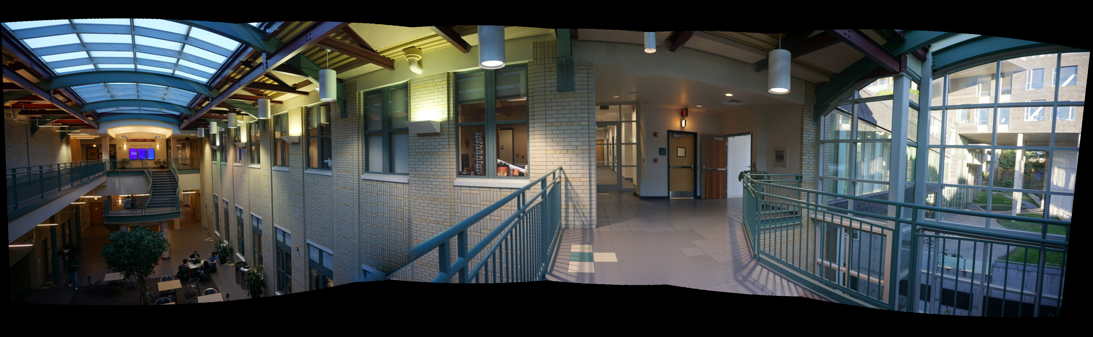
(b)

Figure 12: BRAS panoramic composition for a dataset with a long image sequence. Top: $6$ images from the CMU dataset [56]. Bottom: The final panoramic composition as achieved by BRAS after alignment and stitching.

IV-F Panoramic Stitching Comparisons

We compare BRAS against recent state-of-the-art methods, including AutoStitch [9], APAP [12], CPW [24], and SPHP [21]. We also include a cutting-edge commercial software, Microsoft ICE [57]. We carry out the comparisons over a large variety of image datasets, all taken from recent publications in the literature of image alignment and stitching. Because CPW can only handle pairwise image stitching directly, we only include its results for the two-image cases.

IV-F1 Qualitative Evaluation on Image Stitching

Fig. 14 shows the aligned images on the railtracks dataset [12]. The stitched version may be found in the supplementary document. From the insets, we find that BRAS achieves a superior alignment accuracy than the others, as evidenced by its significantly reduced ghosting artifacts.

Fig. 15 shows an additional alignment example on the skyscraper dataset [21]. From the insets, it is clear that BRAS aligns the edges and lines more accurately compared with both SPHP and APAP, and is free from structural distortions which are evident in APAP.

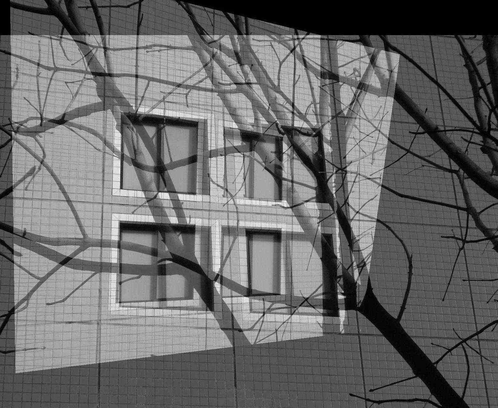
(a) SIFT

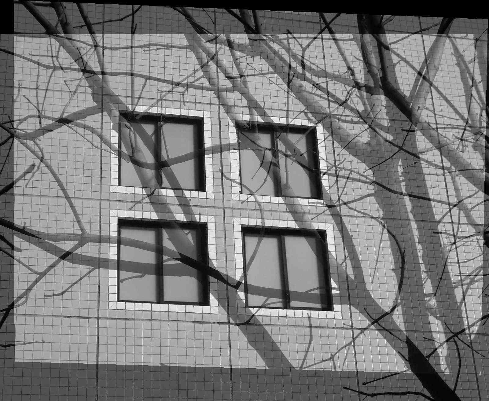
(b) BRAS

​​

Figure 13: Alignment results under large occlusions. LABEL:sub@fig:winSIFT A representative feature-based method (using SIFT) generates misaligned results because of large occlusions. LABEL:sub@fig:winBRAS BRAS accurately aligns the images. Images are from [3].

Fig. 17 shows stitched images for the apartments image set [13]. To show the artifacts we magnify some regions. AutoStitch, ICE and SPHP are based on the single homography model, and thus they perform poorly whenever this simple model is inadequate. Compared with them, CPW and APAP employ multiple homographies and are more flexible, but severe artifacts such as shape distortions still remain. In contrast, the result of BRAS is significantly more visually appealing. Additionally, the aligned version (in the supplementary document) shows that BRAS succeeds in finding a more accurate and sensible alignment than the others.

Finally, we include the stitched images for the hanger image set [14] in Fig. 16. As highlighted in the red circles, AutoStitch and SPHP bend the lines on the wall, while AutoStitch, ICE and SPHP duplicate part of the bed frame. APAP and CPW perform better, but the bed frame is distorted by both methods, and appears broken in their stitched results. The result of BRAS, on the other hand, is clearly of higher visual quality and free from the aforementioned artifacts.

(a) CPW [24]

(b) SPHP [21]

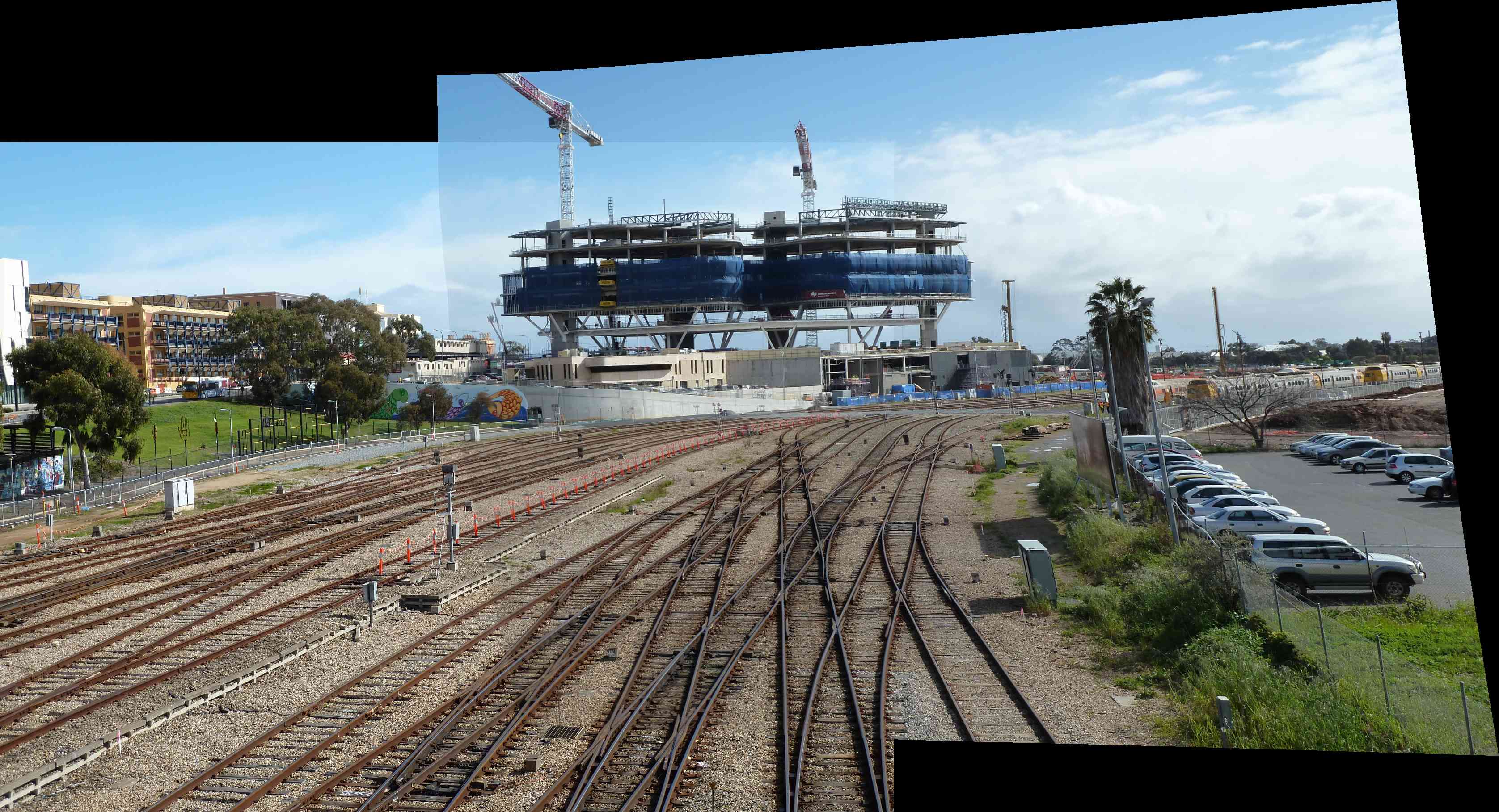
(d) BRAS

​
​

(c) APAP [12]

Figure 14: Aligned and overlayed images on the railtracks dataset [12]. Regions with misalignments are magnified in the insets at the bottom. Please notice the ghosting artifacts produced by LABEL:sub@fig:railtracks_CPW CPW LABEL:sub@fig:railtracks_SPHP SPHP and LABEL:sub@fig:railtracks_APAP APAP, which indicate alignment errors and do not appear in LABEL:sub@fig:railtracks_BRAS BRAS.

(a) SPHP [21]

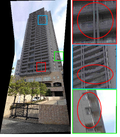
(b) APAP [12]

(c) BRAS

​  ​

Figure 15: Aligned and overlayed images on the skyscraper dataset [21]. Red circles highlight errors and ghosting indicates misalignments.

(a) AutoStitch [9]

(b) ICE [57]

(c) CPW [24]

​  ​

(d) SPHP [21]

(e) APAP [12]

(f) BRAS

​  ​

Figure 16: Stitched images on the hanger dataset [14]. Red circles in the insets highlight artifacts.

(a) AutoStitch [9]

(b) ICE [57]

(c) CPW [24]

​  ​

(d) SPHP [21]

(e) APAP [12]

(f) BRAS

​  ​

Figure 17: Qualitative comparison on the stitched images of the apartments dataset [13]. Regions with artifacts are magnified in the insets and circled in red at the bottom. In particular, please notice the duplicated windows in the stitched images of LABEL:sub@fig:apartments_ICE ICE, LABEL:sub@fig:apartments_SPHP SPHP, and LABEL:sub@fig:apartments_APAP APAP (in the blue insets). Also notice the ghosting, line distortion, and misplacement artifacts in the stitched images of LABEL:sub@fig:apartments_autostitch AutoStitch, LABEL:sub@fig:apartments_CPW CPW and LABEL:sub@fig:apartments_SPHP SPHP (in the green insets).

IV-F2 Quantitative Evaluation of Alignment Accuracy

The truncated $\ell_{2}$-norm for several image sets processed by different algorithms are presented in Table II. The corresponding stitched images (other than those already shown) can be found in the supplementary document. The best results are highlighted and “-” stands for the case where the corresponding algorithm is not capable of handling multiple images. It can be observed that BRAS consistently achieves the best performance, and usually outperforms other algorithms by a clear margin. We note here again that the underlying motion model for BRAS is essentially the same as APAP; thus its improved accuracy is attributable to its improved model fitting strategy which crucially relies on exact capture of the rank. Furthermore, this confirms the intuition that pixel-based method can achieve superior accuracy as BRAS is of pixel-based nature (as discussed in Section II-D).

TABLE II: Alignment accuracies of different methods on each dataset, measured in truncated $\ell_{2}$ norm. Lower values typically indicate higher accuracies.

Dataset	BRAS	APAP [12]	CPW [24]	SPHP [21]
skyscraper [21]	$\mathbf{16.83}$	$17.21$	$-$	$17.40$
railtracks [12]	$\mathbf{16.74}$	$17.67$	$18.13$	$19.23$
apartments [13]	$\mathbf{14.88}$	$16.68$	$15.92$	$17.45$
rooftops [14]	$\mathbf{16.61}$	$17.09$	$-$	$17.37$
forest [12]	$\mathbf{20.53}$	$20.83$	$-$	$20.75$
carpark [13]	$\mathbf{13.99}$	$15.51$	$16.67$	$16.52$
temple [13]	$\mathbf{12.70}$	$14.00$	$14.72$	$14.43$
hanger [14]	$\mathbf{7.61}$	$8.15$	$9.41$	$10.44$
couch [14]	$\mathbf{13.24}$	$13.75$	$13.92$	$14.51$

Finally, we compare in Fig. 18 the running time of each algorithm on all the datasets included in Table II. In particular, Fig. 18 plots the average running times against the total number of pixels in each dataset. The running time for BRAS includes every stage illustrated in Fig. 3 as described in Section III-A to Section III-C. AutoStitch and ICE are not included since they are commercial softwares. We employ a computer with an Intel Core i5–6200, 2.30GHz CPU and 8GB of RAM. SPHP usually runs the fastest, while BRAS usually ranks the second. Moreover, BRAS scales well when the image resolution increases. Note that the couch image set (with around $2\times 10^{7}$ pixels) has relatively small motion and thus all methods run faster on it.

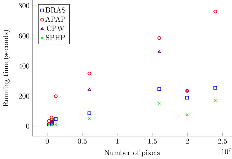
Figure 18: Running time of different methods on each dataset in Table II.

IV-G Stitching in the Presence of Large Moving Objects

One of the most difficult cases for panoramic alignment and stitching is when large moving objects are present in the image set. The catabus image set [58] shown in Fig. 19a represents such a case. Note that this example is representative of scenarios where feature based methods are unlikely to work well. This is because there is a large moving object in the foreground with significant motion (the bus) while the background is relatively simple. That is, feature based methods must largely rely on the moving object features for alignment and the large motion means that the accuracy of the alignment is fundamentally limited.

Fig. 19 shows the stitched image results generated using different methods. The corresponding aligned images are in the supplementary document. Figs. 19b, 19c and 19d, show results of the most competitive feature based methods, ICE, CPW and APAP respectively. Distortions due to misalignment can be seen in the yellow line on the road and the duplication of a tree can be easily identified. In contrast, being pixel based, BRAS bases its alignment on common overlapping regions between the two images in the catabus set, where the accuracy of the said alignment is enabled by the rank-1 and sparse decomposition. It is readily apparent from Fig. 19e that BRAS composes a realistic stitched image free of the distortions in Figs. 19 (b), (c) and (d).

(a) Input

(b) ICE [57]

(c) CPW [24]

(d) APAP [12]

(e) BRAS

Figure 19: Stitching results for catabus dataset [58] – the case with large moving objects. The red circles highlight line distortions and tree duplication in LABEL:sub@fig:catabusICE ICE, LABEL:sub@fig:catabusCPW CPW and LABEL:sub@fig:catabusAPAP APAP, which are absent in LABEL:sub@fig:catabusBRAS BRAS.

IV-H Limitations and Future Works

For our implementation, we integrate the geometric transformation model proposed in [12] for its simplicity and relatively high accuracy. Nevertheless, visual aspects such as shape/structure preservation were not considered in [12], and shape/structure distortions may appear in the stitched images, especially around non-overlapping regions. Similarly, our method may exhibit such drawbacks as well, as can be seen in Fig. 14d and Fig. 17f, etc. However, our contributions are complementary to those works that focus on improving the geometric transformation models, and our framework can be flexibly combined with recently developed geometric models. Therefore, addressing shape/structure distortions by integrating in the BRAS framework, models such as those in [21, 25] is an interesting direction of future exploration.

V Conclusion

We develop a new bundle robust alignment method for panoramic stitching (BRAS). We formulate the alignment problem as the recovery of a rank-1 matrix under sparse corruptions in the transformation domain, and develop efficient algorithms and theoretical guarantees, together with important generalizations to handle realistic scenarios. Unlike most of the existing algorithms that employ feature matching, our method works directly on pixels. In contrast with other panoramic alignment techniques based on matrix decompositions, exactly forcing a rank-1 constraint (vs. existing convex relaxations) plays a crucial role in ensuring practical successes. Extensive experiments confirm that BRAS aligns more accurately and often achieves better visual quality of panoramic stitched images than many state-of-the art techniques.

Supplementary Document

VI Proof of the Key Induction Step

TABLE III: Partial list of symbols and their concise meanings used in Section VI and Section II. Please refer to the text for detailed explanations. For some other standard definitions, please refer to the Notation part of Section II.

Symbols	Space	Meanings
$m$	Integers	Number of pixels on canvas
$n$	Integers	Number of images
$h,w$	Integers	Dimension of the canvas
$d$	Integers	Number of transformation parameters per image; equals $8$ for the single homography case
$\beta_{0},\beta_{1},\zeta,q$	$\mathbb{R}$	Positive constant parameters
$\tau$	$\mathbb{R}^{d\times n}$	Geometric transformation parameters; represent plane homographies unless otherwise stated
$\Delta\tau$	$\mathbb{R}^{d\times n}$	Incremental transformation parameters
${\bf D}$	$\mathbb{R}^{m\times n}$	Data matrix: images stacked as columns
${\bf L}$	$\mathbb{R}^{m\times n}$	Rank-1 component
${\bf S}$	$\mathbb{R}^{m\times n}$	Sparse component modeling errors
${\bf J}_{i}$	$\mathbb{R}^{m\times d}$	Jacobian of image $i$ with respect to its transformation parameters $\tau_{i}$
${\bf Q}_{i},{\bf R}_{i}$	$\mathbb{R}^{m\times d},\mathbb{R}^{d\times d}$	QR decomposition of ${\bf J}_{i}$

Algorithm 4 Alternating Minimization for Solving Linearized Subproblem (Single Overlapping Case)

0:  ${\bf D}_{\tau}\in\mathbb{R}^{m\times n}$, ${\{{\bf J}_{i}\in\mathbb{R}^{m\times d}\}}_{i=1}^{n}$,$\beta_{0}$,$\beta_{1}>0$,$q\in(0,1)$.

1:  ${\bf L}^{0}\leftarrow 0$,$\Delta\tau^{0}\leftarrow 0$,$\zeta_{0}=\beta_{0}\frac{\|{\bf D}_{\tau}\|_{2}}{\sqrt{mn}}$,${\bf S}^{0}\leftarrow{\mathcal{S}}_{\zeta_{0}}({\bf D}_{\tau})$.

2:  for $k=1,2,\dots,K$ do

3:     ${\bf L}^{k}\leftarrow{\mathcal{T}}_{1}\left\{{\bf D}_{\tau}+\sum_{i=1}^{n}{\bf J}_{i}\Delta\tau_{i}^{k-1}{\bf e}_{i}^{T}-{\bf S}^{k-1}\right\}$,

4:     $\zeta_{k}\leftarrow\beta_{1}\frac{q^{k}}{\sqrt{mn}}\|{\bf L}^{k}\|_{2}$,

5:     ${\bf S}^{k}\leftarrow{\mathcal{S}}_{\zeta_{k}}\left\{{\bf D}_{\tau}+\sum_{i=1}^{n}{\bf J}_{i}\Delta\tau_{i}^{k-1}{\bf e}_{i}^{T}-{\bf L}^{k}\right\}$,

6:     $\Delta\tau^{k}\leftarrow\sum_{i=1}^{n}{\bf J}_{i}^{\dagger}({\bf L}^{k}+{\bf S}^{k}-{\bf D}_{\tau}){\bf e}_{i}{\bf e}_{i}^{T}$.

7:  end for

7:  $\widehat{{\bf L}}\leftarrow{\bf L}^{K}$, $\widehat{{\bf S}}\leftarrow{\bf S}^{K}$, $\widehat{\Delta\tau}\leftarrow\Delta\tau^{K}$.

This section is devoted to the proof of the key induction step along the proof of Theorem 7. Our goal is to prove $l_{k+1}\leq\frac{1}{16\mu\nu\sqrt{d}}\frac{\sigma^{\ast}q^{k+1}}{\sqrt{n}}$, ${\mathrm{Supp}}({\bf S}^{k+1})\subset{\mathrm{Supp}}({\bf S}^{\ast})$ and $s_{k+1}\leq\frac{5\widetilde{\mu}\sigma^{\ast}q^{k+1}}{\sqrt{mn}}$ assuming $l_{k}\leq\frac{1}{16\mu\nu\sqrt{d}}\frac{\sigma^{\ast}q^{k}}{\sqrt{n}}$, ${\mathrm{Supp}}({\bf S}^{k})\subset{\mathrm{Supp}}({\bf S}^{\ast})$ and $s_{k}\leq\frac{5\widetilde{\mu}\sigma^{\ast}q^{k}}{\sqrt{mn}}$ where $s_{k}:=\|{\bf E}^{k}\|_{\ell_{\infty}}$ and $l_{k}:=\max_{i}\|{\bf G}^{k}{\bf e}_{i}\|_{\ell_{2}}$. We copy Algorithm 1 in the paper here as Algorithm 4 for easier reference. We also list some of the symbols and notations in Table III. Let us define ${\bf M}^{k}={\bf H}^{k}+{\bf E}^{k}$. We first prove four technical lemmas:

Lemma 1.

For $\ k\geq 0$, if ${\mathrm{Supp}}({\bf E}^{k})\subset{\mathrm{Supp}}({\bf S}^{\ast})$, then

$$\|{\bf Q}_{i}^{T}{\bf E}^{k}{\bf e}_{l}\|_{\ell^{2}}\leq\nu\alpha_{1}\sqrt{md}s_{k},\forall i,l=1,2,\dots,n.$$

Proof.

Since ${\bf E}^{k}$ has at most $\alpha_{1}$ fraction of non-zeros in each column (A.3), using Cauchy-Schwartz inequality,

$$\|{\bf Q}_{i}^{T}{\bf E}^{k}{\bf e}_{l}\|_{\ell^{2}}^{2} =\sum_{j_{1}=1}^{m}\sum_{j_{2}=1}^{m}{\bf e}_{l}^{T}{({\bf E}^{k})}^{T}{\bf e}_{j_{1}}{\bf e}_{j_{1}}^{T}{\bf Q}_{i}{\bf Q}_{i}^{T}{\bf e}_{j_{2}}{\bf e}_{j_{2}}^{T}{\bf E}^{k}{\bf e}_{l}$$

$$\leq\sum_{j_{1},j_{2}}|{({\bf E}^{k})}_{j_{1},l}||{({\bf E}^{k})}_{j_{2},l}|{\left(\max_{1\leq l\leq m}\|{\bf Q}_{i}^{T}{\bf e}_{l}\|_{\ell^{2}}\right)}^{2}$$

$$\leq{\left(\alpha_{1}m\|{\bf E}^{k}\|_{\ell^{\infty}}\right)}^{2}{\left(\nu\sqrt{\frac{d}{m}}\right)}^{2}={\left(\nu\alpha_{1}\sqrt{md}s_{k}\right)}^{2}.$$

∎

Lemma 2.

For $i=1,2,\dots,n$, $\forall{\bf v}\in\mathbb{R}^{n}$ and $k\geq 0$, if ${\mathrm{Supp}}({\bf E}^{k})\subset{\mathrm{Supp}}({\bf S}^{\ast})$, $n\geq 5\mu^{2}$, $0<\delta\leq\frac{1}{20\mu^{2}}$, then

$$\|{\bf Q}_{i}^{T}{\bf M}^{k}{\bf v}\|_{\ell^{2}}\leq\left(\frac{1}{4\mu^{2}}l_{k}+\frac{5}{4}\alpha_{1}\nu\sqrt{md}s_{k}\right)n\|{\bf v}\|_{\ell^{\infty}}.$$

Proof.

Under our choice of $\delta$, $1+(n-1)\delta\leq\frac{n}{4\mu^{2}}$; thus $n+1+(n-1)\delta\leq\frac{5}{4}n$ since $\mu\geq 1$. Therefore,

$$\|{\bf Q}_{i}^{T}{\bf G}^{k}{\bf v}\|_{\ell^{2}}\leq \|{\bf Q}_{i}^{T}{\bf G}^{k}{\bf e}_{i}\|_{\ell^{2}}|{({\bf v})}_{i}|+\sum_{j\neq i}\|{\bf Q}_{i}^{T}{\bf Q}_{j}{\bf Q}_{j}^{T}{\bf G}^{k}{\bf e}_{j}\|_{\ell^{2}}|{({\bf v})}_{j}|$$

$$\leq l_{k}\|{\bf v}\|_{\ell^{\infty}}+\left(\sum_{j\neq i}\|{\bf Q}_{i}^{T}{\bf Q}_{j}\|_{2}\right)l_{k}\|{\bf v}\|_{\ell^{\infty}}\leq[1+(n-1)\delta]l_{k}\|{\bf v}\|_{\ell^{\infty}}\leq\frac{n}{4\mu^{2}}l_{k}\|{\bf v}\|_{\ell^{\infty}},$$ (23)

$$\|{\bf Q}_{i}^{T}{\bf F}^{k}{\bf v}\|_{\ell^{2}}\leq [1+(n-1)\delta]\left(\max_{1\leq i\leq n}\|{\bf Q}_{i}^{T}{\bf E}^{k}{\bf e}_{i}\|_{2}\right)\|{\bf v}\|_{\ell^{\infty}}$$

$$\stackrel{{\scriptstyle\mbox{\tiny Lemma 2}}}{{\leq}} [1+(n-1)\delta](\alpha_{1}\nu\sqrt{md}s_{k})\|{\bf v}\|_{\ell^{\infty}},$$ (24)

$$\|{\bf Q}^{T}_{i}{\bf E}^{k}{\bf v}\|_{\ell^{2}}^{2} =\sum_{j_{1}=1}^{m}\sum_{j_{2}=1}^{m}{\bf v}^{T}{({\bf E}^{k})}^{T}{\bf e}_{j_{1}}{\bf e}_{j_{1}}^{T}{\bf Q}_{i}{\bf Q}_{i}^{T}{\bf e}_{j_{2}}{\bf e}_{j_{2}}^{T}{\bf E}^{k}{\bf v}$$

$$\leq\sum_{j_{1},j_{2}}{\left(\max_{1\leq j\leq m}\|{\bf Q}_{i}^{T}{\bf e}_{j}\|_{\ell^{2}}\right)}^{2}\left|{\bf e}_{j_{1}}^{T}{\bf E}^{k}{\bf v}\right|\left|{\bf e}_{j_{2}}^{T}{\bf E}^{k}{\bf v}\right|$$

$$\leq{\left(\nu\sqrt{\frac{d}{m}}\right)}^{2}{\left(\sum_{i=1}^{n}\sum_{j=1}^{m}{({\bf E}^{k})}_{ji}{({\bf v})}_{i}\right)}^{2}$$

$$={\left(\alpha_{1}\nu n\sqrt{md}s_{k}\|{\bf v}\|_{\ell^{\infty}}\right)}^{2}.$$ (25)

Adding (23), (24), (25) up gives the result. ∎

Lemma 3.

For $k\geq 0$, if ${\mathrm{Supp}}({\bf E}^{k})\subset{\mathrm{Supp}}({\bf S}^{\ast})$, then $\forall{\bf v}\in\mathbb{R}^{n}$

$$\|{\bf M}^{k}{\bf v}\|_{\ell^{\infty}}\leq\left[\nu\sqrt{\frac{d}{m}}l_{k}+(\alpha_{2}+\alpha_{1}\nu^{2}d)s_{k}\right]n\|{\bf v}\|_{\ell^{\infty}}.$$

Proof.

$\forall i$, adding the following inequalities up

$$\left|{\bf e}_{i}^{T}{\bf G}^{k}{\bf v}\right| \leq\sum_{j=1}^{n}\|{\bf e}_{i}^{T}{\bf Q}_{j}\|_{\ell^{2}}\|{\bf Q}_{j}^{T}{\bf G}^{k}{\bf e}_{j}\|_{\ell^{2}}|{({\bf v})}_{j}|$$

$$\leq n\nu\sqrt{\frac{d}{m}}l_{k}\|{\bf v}\|_{\ell^{\infty}},$$

$$|{\bf e}_{i}^{T}{\bf E}^{k}{\bf v}| \leq\|{\bf E}^{k}\|_{\infty}\|{\bf v}\|_{\ell^{\infty}}\leq\alpha_{2}ns_{k}\|{\bf v}\|_{\ell^{\infty}},$$

$$|{\bf e}_{i}^{T}{\bf F}^{k}{\bf v}| \leq\nu\sqrt{\frac{d}{m}}\left(\max_{1\leq j\leq n}\|{\bf Q}_{j}^{T}{\bf E}^{k}{\bf e}_{j}\|_{\ell^{2}}\right)n\|{\bf v}\|_{\ell^{\infty}}$$

$$\leq n\nu\sqrt{\frac{d}{m}}(\alpha_{1}\nu\sqrt{md}s_{k})\|{\bf v}\|_{\ell^{\infty}}=\alpha_{1}\nu^{2}nds_{k}\|{\bf v}\|_{\ell^{\infty}}.$$

and taking maximum over $i$ gives the desired result. ∎

Lemma 4.

$\forall k\geq 0$, if ${\mathrm{Supp}}({\bf E}^{k})\subset{\mathrm{Supp}}({\bf S}^{\ast})$, then $\forall{\bf u}\in\mathbb{R}^{m}$

$$\left\|{({\bf M}^{k})}^{T}{\bf u}\right\|_{\ell^{\infty}}\leq\left[\nu\sqrt{\frac{d}{m}}l_{k}+\alpha_{1}(1+\nu^{2}d)s_{k}\right]m\|{\bf u}\|_{\ell^{\infty}}.$$

Proof.

For $i=1,\dots,n$, using Cauchy-Schwartz inequality,

$$\left\|{\bf Q}_{i}^{T}{\bf u}\right\|_{\ell^{2}}^{2} =\sum_{j_{1}=1}^{m}\sum_{j_{2}=1}^{m}{\bf u}^{T}{\bf e}_{j_{1}}{\bf e}_{j_{1}}^{T}{\bf Q}_{i}{\bf Q}_{i}^{T}{\bf e}_{j_{2}}{\bf e}_{j_{2}}^{T}{\bf u}$$

$$\leq m^{2}{\left(\nu\sqrt{\frac{d}{m}}\right)}^{2}\|{\bf u}\|_{\ell^{\infty}}^{2}={(\nu\sqrt{md}\|{\bf u}\|_{\ell^{\infty}})}^{2}.$$

Lemma 4 comes from adding the following inequalities

$$|{\bf e}_{i}^{T}{({\bf G}^{k})}^{T}{\bf u}| =|{\bf e}_{i}^{T}{({\bf L}^{k}-{\bf L}^{\ast})}^{T}{\bf Q}_{i}{\bf Q}_{i}^{T}{\bf u}|\leq l_{k}\|{\bf Q}_{i}^{T}{\bf u}\|_{\ell^{2}}\leq l_{k}\nu\sqrt{md}\|{\bf u}\|_{\ell^{\infty}},$$

$$|{\bf e}_{i}^{T}{({\bf F}^{k})}^{T}{\bf u}| \leq\left(\max_{1\leq i\leq n}\|{\bf Q}_{i}^{T}{\bf E}^{k}{\bf e}_{i}\|_{\ell^{2}}\right)\left(\max_{1\leq i\leq n}\|{\bf Q}_{i}^{T}{\bf u}\|_{\ell^{2}}\right)\leq\alpha_{1}\nu^{2}mds_{k}\|{\bf u}\|_{\ell^{\infty}},$$

$$|{\bf e}_{i}^{T}{({\bf E}^{k})}^{T}{\bf u}| \leq\|{\bf E}^{k}\|_{1}\|{\bf u}\|_{\ell^{\infty}}\leq\alpha_{1}ms_{k}\|{\bf u}\|_{\ell^{\infty}},$$

and taking the maximum over $i$. ∎

We now start the major procedures. From step 6 in Algorithm 4,

$$\sum_{i=1}^{n}{\bf J}_{i}(\Delta\tau^{k}-\Delta\tau^{\ast}){\bf e}_{i}{\bf e}_{i}^{T}=\sum_{i=1}^{n}{\bf Q}_{i}{\bf Q}_{i}^{T}({\bf L}^{k}-{\bf L}^{\ast}+{\bf S}^{k}-{\bf S}^{\ast}){\bf e}_{i}{\bf e}_{i}^{T}={\bf H}^{k}.$$

Therefore, from step 3 in Algorithm 4

$$\sigma_{1}{\bf u}_{1} =\sigma^{\ast}({{\bf v}^{\ast}}^{T}{\bf v}_{1}){\bf u}^{\ast}+{\bf M}^{k}{\bf v}_{1},$$ (26)

$$\sigma_{1}{\bf v}_{1}^{T} =\sigma^{\ast}({\bf u}_{1}^{T}{\bf u}^{\ast}){{\bf v}^{\ast}}^{T}+{\bf u}_{1}^{T}{\bf M}^{k}.$$ (27)

where ${\bf L}^{k+1}=\sigma_{1}{\bf u}_{1}{\bf v}_{1}^{T}$ is the SVD of ${\bf L}^{k+1}$. Thus

$$\frac{\sigma^{\ast}({{\bf v}^{\ast}}^{T}{\bf v}_{1})({{\bf u}^{\ast}}^{T}{\bf u}_{1})}{\sigma_{1}}-1 =-\frac{{\bf u}_{1}^{T}{\bf M}^{k}{\bf v}_{1}}{\sigma_{1}},$$

$${\bf L}^{k+1}-{\bf L}^{\ast} =\sigma_{1}{\bf u}_{1}{\bf v}_{1}^{T}-\sigma^{\ast}{\bf u}^{\ast}{{\bf v}^{\ast}}^{T}$$

$$=-\frac{{\bf u}_{1}^{T}{\bf M}^{k}{\bf v}_{1}}{\sigma_{1}}\sigma^{\ast}{\bf u}^{\ast}{{\bf v}^{\ast}}^{T}+\frac{\sigma^{\ast}({{\bf v}^{\ast}}^{T}{\bf v}_{1}){\bf u}^{\ast}{\bf u}_{1}^{T}{\bf M}^{k}}{\sigma_{1}}+\frac{\sigma^{\ast}({\bf u}_{1}^{T}{\bf u}^{\ast}){\bf M}^{k}{\bf v}_{1}{{\bf v}^{\ast}}^{T}}{\sigma_{1}}+\frac{{\bf M}^{k}{\bf v}_{1}{\bf u}_{1}^{T}{\bf M}^{k}}{\sigma_{1}}.$$ (28)

By right multiplying (27) with ${({\bf M}^{k})}^{T}$ and plugging it into (26)

$$\sigma_{1}^{2}{\bf u}_{1}-{\bf M}^{k}{({\bf M}^{k})}^{T}{\bf u}_{1}=\sigma_{1}\sigma^{\ast}{\bf u}^{\ast}({{\bf v}^{\ast}}^{T}{\bf v}_{1})+\sigma^{\ast}({\bf u}_{1}^{T}{\bf u}^{\ast}){\bf M}^{k}{\bf v}^{\ast},$$ (29)

The induction hypotheses assures ${\mathrm{Supp}}({\bf E}^{k})\subset{\mathrm{Supp}}({\bf S}^{\ast})$ and

$$l_{k}\leq\frac{1}{16\mu\nu\sqrt{d}}\frac{\sigma^{\ast}}{\sqrt{n}},s_{k}\leq 5\widetilde{\mu}\frac{\sigma^{\ast}}{\sqrt{mn}};$$

from step 3 in Algorithm 4 and the inequalities

$$\|{\bf E}^{k}\|_{2} \leq\sqrt{\|{\bf E}^{k}\|_{1}\|{\bf E}^{k}\|_{\infty}},$$

$$\|{\bf H}^{k}\|_{F}^{2} =\sum_{i=1}^{n}\|{\bf G}^{k}{\bf e}_{i}\|_{\ell^{2}}^{2}+\|{\bf F}^{k}{\bf e}_{i}\|_{\ell^{2}}^{2}\stackrel{{\scriptstyle\mbox{\tiny Lemma 1}}}{{\leq}}nl_{k}^{2}+n{\left(\alpha_{1}\nu\sqrt{md}s_{k}\right)}^{2}$$

we have

$$|\sigma_{1}-\sigma^{\ast}| \leq\|{\bf M}^{k}\|_{2}\leq\sqrt{\|{\bf E}^{k}\|_{1}\|{\bf E}^{k}\|_{\infty}}+\|{\bf H}^{k}\|_{F}$$

$$\leq\sqrt{\alpha_{1}\alpha_{2}mn}s_{k}+\sqrt{n}l_{k}+\sqrt{n}\alpha_{1}\nu\sqrt{md}s_{k}$$ (30)

$$\leq\sigma^{\ast}\left[\frac{1}{16\mu\nu\sqrt{d}}+5\widetilde{\mu}\sqrt{\alpha_{1}}(\sqrt{\alpha_{2}}+\nu\sqrt{\alpha_{1}d})\right]\leq\frac{\sigma^{\ast}}{8},$$

whenever $\alpha_{1}\leq\frac{1}{160\widetilde{\mu}\nu\sqrt{d}}$ and $\alpha_{2}\leq\frac{1}{160\widetilde{\mu}}$. Thus we obtain

$$\frac{8}{9}\leq\frac{\sigma^{\ast}}{\sigma_{1}}\leq\frac{8}{7}.$$ (31)

We next prove that ${\bf u}_{1}$ and ${\bf v}_{1}$ are also incoherent vectors. Indeed, from (29), taking $\|\cdot\|_{\ell^{\infty}}$ on both sides yields

$$\sigma_{1}^{2}\|{\bf u}_{1}\|_{\ell^{\infty}}-\left\|{\bf M}^{k}{({\bf M}^{k})}^{T}{\bf u}_{1}\right\|_{\ell^{\infty}}\leq\sigma_{1}\sigma^{\ast}\|{\bf u}^{\ast}\|_{\ell^{\infty}}+\sigma^{\ast}\left\|{\bf M}^{k}{\bf v}^{\ast}\right\|_{\ell^{\infty}}.$$ (32)

Using Lemma 4 with $\alpha_{1}\leq\frac{1}{40\widetilde{\mu}(1+\nu^{2}d)}$,

$$\|{({\bf M}^{k})}^{T}{\bf u}_{1}\|_{\ell^{\infty}}\leq\sqrt{\frac{m}{n}}\left[\frac{1}{16\mu}+5\alpha_{1}(1+\nu^{2}d)\widetilde{\mu}\right]\sigma^{\ast}\|{\bf u}_{1}\|_{\ell^{\infty}}\leq\frac{1}{4}\sqrt{\frac{m}{n}}\sigma^{\ast}\|{\bf u}_{1}\|_{\ell^{\infty}},$$

and Lemma 3 with $\alpha_{1}\leq\frac{1}{80\nu^{2}d\widetilde{\mu}}$, $\alpha_{2}\leq\frac{1}{80\widetilde{\mu}}$,

$$\left\|{\bf M}^{k}{({\bf M}^{k})}^{T}{\bf u}_{1}\right\|_{\ell^{\infty}} \leq\frac{{\sigma^{\ast}}^{2}}{16}\sqrt{\frac{n}{m}}\sqrt{\frac{m}{n}}\|{\bf u}_{1}\|_{\ell^{\infty}},$$ (33)

$$\left\|{\bf M}^{k}{\bf v}^{\ast}\right\|_{\ell^{\infty}} \leq\frac{\sigma^{\ast}}{4}\sqrt{\frac{n}{m}}\|{\bf v}^{\ast}\|_{\ell^{\infty}}\leq\frac{\mu\sigma^{\ast}}{4\sqrt{m}}.$$ (34)

Plugging (33) and (34) into (32) to obtain (similarly for ${\bf v}_{1}$)

$$\|{\bf u}_{1}\|_{\ell^{\infty}}\leq\frac{2\mu}{\sqrt{m}},\|{\bf v}_{1}\|_{\ell^{\infty}}\leq\frac{2\mu}{\sqrt{n}}.$$ (35)

Now using Lemma 4 again, together with (35)

$$\left\|{({\bf M}^{k})}^{T}{\bf u}_{1}\right\|_{\ell^{\infty}}\leq\left[\frac{1}{8}+2\alpha_{1}\mu(1+\nu^{2}d)c_{s}\right]\frac{\sigma^{\ast}q^{k}}{\sqrt{n}},$$ (36)

where $c_{s}:=5\widetilde{\mu}$. Symmetrically,

$$\|{\bf M}^{k}{\bf v}_{1}\|_{\ell^{\infty}}\leq\left[\frac{1}{8}+2\mu(\alpha_{2}+\alpha_{1}\nu^{2}d)c_{s}\right]\frac{\sigma^{\ast}q^{k}}{\sqrt{m}}.$$ (37)

And using Lemma 2 and (35), by letting $\delta\leq\frac{1}{20\mu^{2}}$,

$$\max_{1\leq i\leq n}\|{\bf Q}_{i}^{T}{\bf M}^{k}{\bf v}_{1}\|_{\ell^{2}}\leq\left(\frac{5}{2}\alpha_{1}\mu\nu\sqrt{d}c_{s}+\frac{1}{32\mu^{2}\nu\sqrt{d}}\right)\sigma^{\ast}q^{k}.$$ (38)

Also, working in the same manner as in (30), we obtain

$$\left|{\bf u}_{1}^{T}{\bf M}^{k}{\bf v}_{1}\right|\leq\|{\bf M}^{k}\|_{2} \leq\sigma^{\ast}q^{k}\left[c_{s}\sqrt{\alpha_{1}}(\sqrt{\alpha_{2}}+\nu\sqrt{\alpha_{1}d})+\frac{1}{16\mu\nu\sqrt{d}}\right].$$ (39)

For $i=1,2,\dots,n$, a combination of (28) (36) (38) (39) yields

$$\left\|{\bf Q}_{i}^{T}({\bf L}^{k+1}-{\bf L}^{\ast}){\bf e}_{i}\right\|_{\ell^{2}}$$

$$\leq \frac{\sigma^{\ast}|{\bf u}_{1}^{T}{\bf M}^{k}{\bf v}_{1}|}{\sigma_{1}}\frac{\kappa\mu\sqrt{d}}{\sqrt{mn}}+\frac{\sigma^{\ast}\kappa}{\sigma_{1}}\sqrt{\frac{d}{m}}\left\|{({\bf M}^{k})}^{T}{\bf u}_{1}\right\|_{\ell^{\infty}}+\frac{\|{\bf Q}_{i}^{T}{\bf M}^{k}{\bf v}_{1}\|_{\ell^{2}}}{\sigma_{1}}\left[\frac{\sigma^{\ast}\mu}{\sqrt{n}}+\left\|{({\bf M}^{k})}^{T}{\bf u}_{1}\right\|_{\ell^{\infty}}\right]$$

$$\leq \frac{8}{7}\biggl{\{}\biggl{[}\frac{1}{16\nu\sqrt{d}}+\frac{1}{8}+c_{s}\mu\biggl{(}\sqrt{\alpha_{1}\alpha_{2}}+2\alpha_{1}\biggl{(}1+\nu^{2}d+\frac{\nu\sqrt{d}}{2}\biggr{)}\biggr{)}\biggr{]}\kappa\sqrt{\frac{d}{m}}+\frac{5}{4}\left(\frac{5}{2}\alpha_{1}\mu^{2}\nu\sqrt{d}c_{s}+\frac{1}{32\mu\nu\sqrt{d}}\right)\biggr{\}}\frac{\sigma^{\ast}q^{k}}{\sqrt{n}},$$ (40)

where in (40) we use (31) and the following inequality

$$\frac{\sigma^{\ast}\mu}{\sqrt{n}}+\|{({\bf M}^{k})}^{T}{\bf u}_{1}\|_{\ell^{\infty}}\leq\frac{\sigma^{\ast}\mu}{\sqrt{n}}\left[1+\left(\frac{1}{8\mu}+2\alpha_{1}(1+\nu^{2}d)c_{s}\right)\right]\leq\frac{\sigma^{\ast}\mu}{\sqrt{n}}\left[1+\left(\frac{1}{8}+\frac{1}{8}\right)\right]\leq\frac{5}{4}\frac{\sigma^{\ast}\mu}{\sqrt{n}},$$

whenever $\alpha_{1}\leq\frac{1}{16c_{s}(1+\nu^{2}d)}$. Now for $\alpha_{1},\alpha_{2}$ sufficiently small (in the order of $\mathcal{O}(d^{-1})$,$\mathcal{O}(d^{-\frac{1}{2}})$, respectively) and $d\leq\frac{\sqrt{m}}{32\mu^{2}\nu\kappa}$, $\exists q<1$ such that (40) becomes

$$l_{k+1}\leq\frac{1}{16\mu\nu\sqrt{d}}\frac{\sigma^{\ast}q^{k+1}}{\sqrt{n}}.$$

On the other hand, using (28) (36) (37) (39),

$$\|{\bf L}^{k+1}-{\bf L}^{\ast}\|_{\ell^{\infty}}$$

$$\leq \frac{\sigma^{\ast}|{\bf u}_{1}^{T}{\bf M}^{k}{\bf v}_{1}|}{\sigma_{1}}\frac{\mu^{2}}{\sqrt{mn}}+\frac{\sigma^{\ast}}{\sigma_{1}}\frac{\mu}{\sqrt{m}}\left\|{({\bf M}^{k})}^{T}{\bf u}_{1}\right\|_{\ell^{\infty}}+\frac{\sigma^{\ast}\|{\bf M}^{k}{\bf v}_{1}\|_{\ell^{\infty}}}{\sigma_{1}}\frac{\mu}{\sqrt{n}}+\frac{\|{\bf M}^{k}{\bf v}_{1}\|_{\ell^{\infty}}\left\|{({\bf M}^{k})}^{T}{\bf u}_{1}\right\|_{\ell^{\infty}}}{\sigma_{1}}$$

$$\leq \frac{\sigma^{\ast}q^{k}\mu^{2}}{\sqrt{mn}}\frac{\sigma^{\ast}}{\sigma_{1}}\biggl{\{}\frac{1}{16\mu\nu\sqrt{d}}+\frac{1}{4\mu}+4\alpha_{1}\nu^{2}dc_{s}+2(\alpha_{1}+\alpha_{2})c_{s}$$

$$+c_{s}(\sqrt{\alpha_{1}\alpha_{2}}+\alpha_{1}\nu\sqrt{d})+\left[\frac{1}{8\mu}+2\alpha_{1}(1+\nu^{2}d)c_{s}\right]\left[\frac{1}{8\mu}+2(\alpha_{2}+\alpha_{1}\nu^{2}d)c_{s}\right]\biggr{\}}$$

$$\leq \frac{\sigma^{\ast}q^{k+1}\mu^{2}}{\sqrt{mn}},$$ (41)

again for some $\alpha_{1},\alpha_{2}$ sufficiently small (same orders as in (40)) and some $q<1$. Under the same conditions,

$$\|{\bf H}^{k}\|_{\ell^{\infty}} \leq\max_{i,j}|{\bf e}_{i}^{T}{\bf Q}_{j}{\bf Q}_{j}^{T}({\bf L}^{k}-{\bf L}^{\ast}+{\bf S}^{k}-{\bf S}^{\ast}){\bf e}_{j}|$$

$$\stackrel{{\scriptstyle\mbox{\tiny Lemma 1}}}{{\leq}}\nu\sqrt{\frac{d}{m}}(l_{k}+\alpha_{1}\nu\sqrt{md}s_{k})\leq\frac{3}{4}\frac{\sigma^{\ast}q^{k+1}\mu^{2}}{\sqrt{mn}},$$

and $|{({\bf L}^{\ast}-{\bf L}^{k+1}+{\bf H}^{k})}_{ij}|\leq\zeta_{k+1},\forall(i,j)\not\in{\mathrm{Supp}}({\bf S}^{\ast})$. From step 5 in Algorithm 4, ${({\bf S}^{k+1})}_{ij}=0$ and ${\mathrm{Supp}}({\bf S}^{k+1})\subset{\mathrm{Supp}}({\bf S}^{\ast})$. Let ${\bf N}^{k}={\bf L}^{\ast}-{\bf L}^{k+1}+{\bf H}^{k}+{\bf S}^{\ast}$, then

$$|{({\bf E}^{k+1})}_{ij}|=|{({\bf S}^{\ast}-{\bf S}^{k+1})}_{ij}|=\begin{cases}|{({\bf L}^{k+1}-{\bf L}^{\ast}-{\bf H}^{k}\pm\zeta_{k+1})}_{ij}|,&\text{ if }|{({\bf N}^{k})}_{ij}|>\zeta_{k+1},\\ |{({\bf S}^{\ast})}_{ij}|,&\text{ if }|{({\bf N}^{k})}_{ij}|\leq\zeta_{k+1}.\end{cases}$$

In both cases $|{({\bf E}^{k+1})}_{ij}|\leq\|{\bf L}^{k+1}-{\bf L}^{\ast}\|_{\ell^{\infty}}+\|{\bf H}^{k}\|_{\ell^{\infty}}+\zeta_{k+1}$ and

$$s_{k+1}\leq 2\zeta_{k+1}=\frac{2\beta_{1}q^{k+1}}{\sqrt{mn}}\sigma_{1}\leq 5\widetilde{\mu}\frac{q^{k+1}}{\sqrt{mn}}\sigma^{\ast}.$$

VII Analysis of Bundle Robust Alignment

In this section we extend our analysis to the case of multiple overlapping regions and derive convergence properties of Algorithm 3. We first introduce the notations and assumptions, analogous to A.1 to A.6 in Section II-C. We then state an extension to Theorem 7 in Section VII-B, followed by the proof. Likewise, the key induction step is postponed to Section VII-C to avoid obscuring the main flow of analysis.

TABLE IV: Partial list of symbols and their concise meanings used in Section VII and Section III. Please refer to the text for detailed explanations. For some other standard definitions, please refer to the Notation part of Section II.

Symbols	Space	Meanings
$s_{1},s_{2}$	$\mathbb{R}^{h_{1}\times w_{1}\times 128},\mathbb{R}^{h_{2}\times w_{2}\times 128}$	SIFT images [2]
$L$	Integers	Maximum pixel displacements
${\bf w}({\bf p})$	${\{-L,-L+1,\dots,L\}}^{2}$	Discretized motion vector at pixel ${\bf p}$
$m$	Integers	Number of pixels on the canvas
$n$	Integers	Number of images
$m_{r}$	Integers	Number of pixels in the $r$-th region
$n_{r}$	Integers	Number of images contributing to the $r$-th region
$\alpha,\beta_{0},\beta_{1},\eta,\kappa,\zeta_{r},q$	$\mathbb{R}$	Positive constant parameters
${\bf D}_{r}$	$\mathbb{R}^{m_{r}\times n_{r}}$	Data matrix for the $r$-th region
${\bf L}_{r}$	$\mathbb{R}^{m_{r}\times n_{r}}$	Rank-1 component in the $r$-th region
${\bf S}_{r}$	$\mathbb{R}^{m_{r}\times n_{r}}$	Sparse component in the $r$-th region
${\bf J}_{r,i}$	$\mathbb{R}^{m_{r}\times d}$	Jacobian of image $i$ in the $r$-th region
$\tau^{(u)}$	$\mathbb{R}^{d\times n}$	Transformation parameters for cell $u$; plane homographies unless otherwise stated
$\Delta\tau^{(u)}$	$\mathbb{R}^{d\times n}$	Incremental transformation parameters for cell $u$
$C_{1},C_{2}$	Integers	Number of cells in row and column

Algorithm 5 Alternating Minimization for Solving Linearized Subproblem (Multiple Overlapping Case)

0:  ${\{{\bf D}_{r}\in\mathbb{R}^{m_{r}\times n_{r}}\}}_{r}$, ${\{{\bf J}_{r,i}\in\mathbb{R}^{m_{r}\times d}\}}_{r,i}$,${\{\beta_{r,0}\}}_{r}$,$\beta_{1}$,$q>0$.

1:  for all $r$ do

2:     ${\bf L}_{r}^{0}\leftarrow 0$, ${\bf S}_{r}^{0}\leftarrow{\mathcal{S}}_{\zeta_{r}^{0}}({\bf D}_{r})$ where $\zeta_{r}^{0}=\beta_{r,0}\frac{\|{\bf D}_{r}\|_{2}}{\sqrt{m_{r}n_{r}}}$.

3:  end for

4:  $\Delta\tau^{0}\leftarrow\sum_{r}\sum_{i\in{\mathcal{I}}_{r}}{\left(\sum_{l\in\bar{{\mathcal{I}}}_{i}}\frac{{\bf J}_{l,i}^{T}{\bf J}_{l,i}}{\zeta_{l}^{0}}\right)}^{\dagger}\frac{{\bf J}_{r,i}^{T}({\bf S}_{r}^{0}-{\bf D}_{r}){\bf e}_{f_{r}^{i}}{\bf e}_{i}^{T}}{\zeta_{r}^{0}}$.

5:  for $k=1,2,\dots,K$ do

6:     for all $r$ do

7:        ${\bf L}_{r}^{k}\leftarrow{\mathcal{T}}_{1}\left\{{\bf D}_{r}+\sum_{i\in\mathcal{I}_{r}}{\bf J}_{r,i}\Delta\tau_{i}^{k-1}{\bf e}_{f_{r}^{i}}^{T}-{\bf S}_{r}^{k-1}\right\}$,

8:        $\zeta_{r}^{k}\leftarrow\beta_{1}\frac{q^{k}}{\sqrt{m_{r}n_{r}}}\|{\bf L}_{r}^{k}\|_{2}$,

9:        ${\bf S}_{r}^{k}\leftarrow{\mathcal{S}}_{\zeta_{r}^{k}}\left\{{\bf D}_{r}+\sum_{i\in\mathcal{I}_{r}}{\bf J}_{r,i}\Delta\tau_{i}^{k-1}{\bf e}_{f_{r}^{i}}^{T}-{\bf L}_{r}^{k}\right\}$.

10:     end for

11:     $\Delta\tau^{k}\leftarrow\sum_{r,i\in{\mathcal{I}}_{r}}\!\!{\left(\sum_{l\in\bar{{\mathcal{I}}}_{i}}\!\!\frac{{\bf J}_{l,i}^{T}{\bf J}_{l,i}}{\zeta_{l}^{k}}\right)}^{\dagger}\!\frac{{\bf J}_{r,i}^{T}({\bf L}_{r}^{k}+{\bf S}_{r}^{k}-{\bf D}_{r}){\bf e}_{f_{r}^{i}}{\bf e}_{i}^{T}}{\zeta_{r}^{k}}$.

12:  end for

12:  $\widehat{{\bf L}_{r}}\leftarrow{\bf L}_{r}^{K}$, $\widehat{{\bf S}_{r}}={\bf S}_{r}^{K}$, $\widehat{\Delta\tau}=\Delta\tau^{K}$.

VII-A Notations

We copy Algorithm 3 in the paper here as Algorithm 5 for easier reference. We also include a summary of the notations and symbols in Table IV. Let ${\bf L}_{r}^{\ast},{\bf S}_{r}^{\ast}$ and $\Delta\tau^{\ast}$ be the true model parameters we aim to recover and ${\bf D}_{r}={\bf L}_{r}^{\ast}+{\bf S}_{r}^{\ast}-\sum_{i\in{\mathcal{I}}_{r}}{\bf J}_{r,i}\Delta\tau_{i}^{\ast}{\bf e}_{f_{r}^{i}}^{T}$ be the data matrices. We assume ${\bf S}_{r}^{\ast}$ has a fraction of at most $\alpha_{r},\alpha_{r}^{\prime}$ non-zeros in each column and row. Let ${\bf L}_{r}^{k+1}=\sigma_{r}{\bf u}_{r}{\bf v}_{r}^{T}$ and ${\bf L}_{r}^{\ast}=\sigma^{\ast}_{r}{\bf u}^{\ast}_{r}{{\bf v}^{\ast}}_{r}^{T}$ be the singular value decomposition of ${\bf L}_{r}^{k+1}$ and ${\bf L}^{\ast}_{r}$, where ${\bf u}_{r},{\bf u}_{r}^{\ast}\in\mathbb{R}^{m_{r}},{\bf v}_{r},{\bf v}_{r}^{\ast}\in\mathbb{R}^{n_{r}}$ are unit vectors. Let ${\bf J}_{r,i}={\bf Q}_{r,i}{\bf R}_{r,i}(i\in{\mathcal{I}}_{r})$ be the (reduced) QR decomposition where ${\bf Q}_{r,i}\in\mathbb{R}^{m_{r}\times d}$ and ${\bf R}_{r,i}\in\mathbb{R}^{d\times d}$; following the same reasoning as in Section II-C, we define positive constants $\mu,\nu,\delta,\kappa,\gamma$ as follows

$$\max_{1\leq i\leq m,j\in{\mathcal{I}}_{r}}\|{\bf Q}_{r,j}^{T}{\bf e}_{i}\|_{\ell^{2}}\leq\nu\sqrt{\frac{d}{m_{r}}},$$

$$\|{\bf u}^{\ast}_{r}\|_{\ell^{\infty}}\leq\frac{\mu}{\sqrt{m_{r}}},\|{\bf v}_{r}^{\ast}\|_{\ell^{\infty}}\leq\frac{\mu}{\sqrt{n_{r}}},$$

$$\frac{1}{n_{r}-1}\sum_{j\neq i}\|{\bf Q}_{r,j}^{T}{\bf Q}_{r,i}\|_{2}\leq\delta,$$

$$\max_{i\in{\mathcal{I}}_{r}}\|{\bf Q}_{r,i}^{T}{\bf u}_{r}^{\ast}\|_{\ell^{2}}\leq\kappa\sqrt{\frac{d}{m_{r}}},\\$$

$$\max_{i\in{\mathcal{I}}_{r}}\|{\bf R}_{r,i}\Delta\tau^{\ast}{\bf e}_{i}\|_{\ell^{2}}\leq\gamma\frac{\sigma_{r}^{\ast}}{\sqrt{n_{r}d}}.$$

Also, ${\mathcal{U}}_{r}:=\bigcup_{i\in{\mathcal{I}}_{r}}\bar{{\mathcal{I}}}_{i}$, $\omega_{r}:=\sum_{t\in{\mathcal{U}}_{r}}\sqrt{\frac{\sigma_{t}^{\ast}}{\sigma_{r}^{\ast}}}\sqrt[4]{\frac{m_{t}n_{r}}{m_{r}n_{t}}}$. Let ${\bf P}_{r,t}^{i,k}={\bf R}_{r,i}{\left[\sum_{l\in\bar{{\mathcal{I}}}_{i}}\frac{{\bf R}_{l,i}^{T}{\bf R}_{l,i}}{\zeta_{l}^{k}}\right]}^{-1}\frac{{\bf R}_{t,i}^{T}}{\zeta_{t}^{k}}$. Let ${\bf E}_{r}^{k}={\bf S}_{r}^{\ast}-{\bf S}_{r}^{k}$, ${\bf F}_{r}^{k}=\sum_{i\in{\mathcal{I}}_{r}}\sum_{t\in\bar{{\mathcal{I}}_{i}}}{\bf Q}_{r,i}{\bf P}_{r,t}^{i,k}{\bf Q}_{t,i}^{T}({\bf S}_{t}^{k}-{\bf S}_{t}^{\ast}){\bf e}_{f_{t}^{i}}{\bf e}_{f_{r}^{i}}$, ${\bf G}_{r}^{k}=\sum_{i\in{\mathcal{I}}_{r}}\sum_{t\in\bar{{\mathcal{I}}_{i}}}{\bf Q}_{r,i}{\bf P}_{r,t}^{i,k}{\bf Q}_{t,i}^{T}({\bf L}_{t}^{k}-{\bf L}_{t}^{\ast}){\bf e}_{f_{t}^{i}}{\bf e}_{f_{r}^{i}}^{T}$, ${\bf H}_{r}^{k}={\bf F}_{r}^{k}+{\bf G}_{r}^{k}$ and ${\bf M}_{r}^{k}={\bf H}_{r}^{k}+{\bf E}_{r}^{k}$. It is easy to check that

$${\bf H}_{r}^{k}=\sum_{i\in{\mathcal{I}}_{r}}{\bf J}_{r,i}(\Delta\tau^{k}-\Delta\tau^{\ast}){\bf e}_{i}{\bf e}_{f_{r}^{i}}^{T}.$$

Therefore, steps 7 and 9 in Algorithm 5 can be rewritten as

$${\bf L}_{r}^{k+1} \leftarrow{\mathcal{T}}_{1}\left\{{\bf M}_{r}^{k}+{\bf L}_{r}^{\ast}\right\},$$ (42)

$${\bf S}_{r}^{k+1} \leftarrow{\mathcal{S}}_{\zeta_{r}^{k+1}}\left\{{\bf L}_{r}^{\ast}-{\bf L}_{r}^{k+1}+{\bf H}_{r}^{k}+{\bf S}_{r}^{\ast}\right\}.$$ (43)

Finally, we define real sequences ${\{l_{r,k}\}}_{k},{\{s_{r,k}\}}_{k}$ as follows

$$l_{r,k}=\max_{i\in{\mathcal{I}}_{r}}\|{\bf Q}_{r,i}^{T}({\bf L}_{r}^{k}-{\bf L}_{r}^{\ast}){\bf e}_{f_{r}^{i}}\|_{\ell^{2}},s_{r,k}=\|{\bf E}_{r}^{k}\|_{\ell^{\infty}}.$$

VII-B Main Result

We are now ready to state the theorem about convergence of Algorithm 5. Basically it asserts that, under certain conditions, the sequences ${\bf L}^{k}_{r},{\bf S}^{k}_{r}$ and $\Delta\tau^{k}$ generated by Algorithm 5 converge to the underlying true model parameters ${\bf L}^{\ast}_{r},{\bf S}^{\ast}_{r}$ and $\Delta\tau^{\ast}$ in a linear rate.

Theorem 2.

Let $\tilde{\alpha_{r}}=\sum_{t\in{\mathcal{U}}_{r}}\alpha_{t}\sqrt{\frac{\sigma_{t}^{\ast}}{\sigma_{r}^{\ast}}}\sqrt[4]{\frac{m_{t}n_{r}}{m_{r}n_{t}}}$. There exist constants $C_{\alpha_{1}}=\mathcal{O}\left(\frac{1}{d}\right)$, $C_{\alpha_{2}}=\mathcal{O}\left(\frac{1}{\sqrt{d}}\right)$, $C_{d}=\mathcal{O}(\sqrt{m})$ and $C_{\delta}$, $C_{q}$, such that if $\tilde{\alpha_{r}}\leq C_{\alpha_{1}}$, $\alpha_{r}^{\prime}\leq C_{\alpha_{2}}$, $d\leq C_{d}$, $\delta\leq C_{\delta}$, $C_{q}\leq q<1$, then $\forall\beta_{r,0}\in\left[\frac{\tilde{\mu}\sigma_{r}^{\ast}}{\|{\bf D}_{r}\|_{2}},\frac{2\tilde{\mu}\sigma_{r}^{\ast}}{\|{\bf D}_{r}\|_{2}}\right]$, $\beta_{1}\in\left[2\tilde{\mu},2.2\tilde{\mu}\right]$ where $\tilde{\mu}=\mu^{2}+\gamma\nu$, each ${\bf S}_{r}^{k}(k=0,1,\dots,K)$ in algorithm 5 has the property ${\mathrm{Supp}}({\bf S}_{r}^{k})\subset{\mathrm{Supp}}({\bf S}_{r}^{\ast})$; furthermore, $\forall\varepsilon>0$, $K\geq\max_{r}\log_{q}\left(\frac{\varepsilon}{\beta_{r,0}\|{\bf D}_{r}\|_{2}}\right)$, $\|\widehat{{\bf L}_{r}}-{\bf L}_{r}^{\ast}\|_{F}\leq\varepsilon$, $\|\widehat{{\bf S}_{r}}-{\bf S}_{r}^{\ast}\|_{\ell^{\infty}}\leq\frac{5\varepsilon}{\sqrt{m_{r}n_{r}}}$ and $\|\widehat{\Delta\tau}-\Delta\tau^{\ast}\|_{F}\leq M\varepsilon$ for some $M>0$.

Proof.

We prove it by induction. Define $l_{0}=\min_{r}\frac{1}{16\omega_{r}\mu\nu\sqrt{d}}$, $s_{0}=5(\mu^{2}+\nu\sqrt{d})$. For $k=0$, $\forall(i,j)\not\in{\mathrm{Supp}}({\bf S}_{r}^{\ast})$, ${({\bf S}_{r}^{\ast})}_{ij}=0$ and

$$|{({\bf D}_{r})}_{ij}| \leq\|{\bf L}_{r}^{\ast}\|_{\ell^{\infty}}+\|\sum_{i\in{\mathcal{I}}_{r}}^{n}{\bf J}_{r,i}\Delta\tau^{\ast}{\bf e}_{i}{\bf e}_{f_{r}^{i}}^{T}\|_{\ell^{\infty}}$$

$$\leq\sigma_{r}^{\ast}\|{\bf u}_{r}^{\ast}\|_{\ell^{\infty}}\|{\bf v}_{r}^{\ast}\|_{\ell^{\infty}}+\max_{i,j}|{\bf e}_{i}^{T}{\bf Q}_{r,i}{\bf R}_{r,i}\Delta\tau^{\ast}{\bf e}_{j}|$$

$$\leq\sigma_{r}^{\ast}\frac{\mu^{2}}{\sqrt{m_{r}n_{r}}}+\nu\sqrt{\frac{d}{m_{r}}}\frac{\sigma_{r}^{\ast}}{\sqrt{n_{r}d}}\gamma\leq\zeta_{r}^{0},$$

and thus ${({\bf S}_{r}^{0})}_{ij}=0$, ${\mathrm{Supp}}({\bf S}_{r}^{0})\subset{\mathrm{Supp}}({\bf S}_{r}^{\ast})$. Furthermore, for $d\leq\min_{r}\frac{\sqrt{m_{r}}}{16\omega_{r}\mu^{2}\nu\kappa}$, $l_{r,0}=\sigma_{r}^{\ast}\max_{i}\|{\bf Q}_{r,i}^{T}{\bf u}_{r}^{\ast}\|_{\ell^{2}}|{({\bf v}_{r}^{\ast})}_{i}|\leq l_{0}\frac{\sigma_{r}^{\ast}}{\sqrt{n_{r}}}$, $\|{\bf L}_{r}^{0}-{\bf L}_{r}^{\ast}\|_{\ell^{\infty}}=\|{\bf L}_{r}^{\ast}\|_{\ell^{\infty}}\leq\frac{\sigma_{r}^{\ast}\mu^{2}}{\sqrt{m_{r}n_{r}}}$ and $s_{r,0}=\|{\bf E}_{r}^{0}\|_{\ell^{\infty}}\leq\zeta_{r}^{0}+\|{\bf L}_{r}^{\ast}\|_{\ell^{\infty}}+\|\sum_{i\in{\mathcal{I}}_{r}}{\bf J}_{r,i}\Delta\tau^{\ast}{\bf e}_{i}{\bf e}_{f_{r}^{i}}^{T}\|_{\ell^{\infty}}\leq s_{0}\frac{\sigma_{r}^{\ast}}{\sqrt{m_{r}n_{r}}}$. Assume that $l_{r,k}\leq l_{0}\frac{\sigma_{r}^{\ast}q^{k}}{\sqrt{n}}$, ${\mathrm{Supp}}({\bf S}_{r}^{k})\subset{\mathrm{Supp}}({\bf S}_{r}^{\ast})$, $\frac{\zeta_{r}^{k}}{\zeta_{t}^{k}}\leq\frac{2\sigma_{r}^{\ast}}{\sigma_{t}^{\ast}}\sqrt{\frac{m_{t}n_{t}}{m_{r}n_{r}}}$ and $s_{r,k}\leq s_{0}\frac{\sigma_{r}^{\ast}q^{k}}{\sqrt{m_{r}n_{r}}}$; our goal is to show $l_{r,k+1}\leq l_{0}\frac{\sigma_{r}^{\ast}q^{k+1}}{\sqrt{n_{r}}}$, ${\mathrm{Supp}}({\bf S}_{r}^{k+1})\subset{\mathrm{Supp}}({\bf S}_{r}^{\ast})$, $\frac{\zeta_{r}^{k+1}}{\zeta_{t}^{k+1}}\leq\frac{2\sigma_{r}^{\ast}}{\sigma_{t}^{\ast}}\sqrt{\frac{m_{t}n_{t}}{m_{r}n_{r}}}$ and $s_{r,k+1}\leq s_{0}\frac{\sigma_{r}^{\ast}q^{k+1}}{\sqrt{m_{r}n_{r}}}$. We delay this procedure to Section VII-C due to its length. For $K\geq\max_{r}\log_{q}\left(\frac{\varepsilon}{\beta_{r,0}\|{\bf D}_{r}\|_{2}}\right)$, as proved in (61), $\|{\bf L}_{r}^{K}-{\bf L}_{r}^{\ast}\|_{\ell^{\infty}}\leq\frac{\mu^{2}\sigma_{r}^{\ast}q^{K}}{\sqrt{m_{r}n_{r}}}\leq\beta_{r,0}\frac{\|{\bf D}_{r}\|_{2}q^{K}}{\sqrt{m_{r}n_{r}}}$ and $\|{\bf S}_{r}^{K}-{\bf S}_{r}^{\ast}\|_{\ell^{\infty}}\leq 5\beta_{r,0}\frac{\|{\bf D}_{r}\|_{2}q^{K}}{\sqrt{m_{r}n_{r}}}$, we have $\|{\bf L}_{r}^{K}-{\bf L}_{r}^{\ast}\|_{F}\leq\varepsilon$, $\|{\bf S}_{r}^{K}-{\bf S}_{r}^{\ast}\|_{\ell^{\infty}}\leq\frac{5\varepsilon}{\sqrt{m_{r}n_{r}}}$; using Lemma 9 in Section VII-C:

$$\|\Delta\tau^{K}-\Delta\tau^{\ast}\|_{F}$$

$$= \sqrt{\sum_{i=1}^{n}\left\|\sum_{r\in\bar{{\mathcal{I}}}_{i}}{\bf R}_{r,i}^{-1}{\bf P}_{r,r}^{i,K}{\bf Q}_{r,i}^{T}({\bf L}_{r}^{K}-{\bf L}_{r}^{\ast}+{\bf S}_{r}^{K}-{\bf S}_{r}^{\ast}){\bf e}_{f_{r}^{i}}\right\|_{\ell^{2}}^{2}}$$

$$\leq \sqrt{\sum_{i=1}^{n}{\left[\sum_{r\in\bar{{\mathcal{I}}}_{i}}\|{\bf R}_{r,i}^{-1}\|_{2}(l_{r,k}+\alpha_{r}\nu\sqrt{m_{r}d}s_{r,k})\right]}^{2}}$$

$$\leq \sqrt{\sum_{i=1}^{n}|\bar{{\mathcal{I}}}_{i}|\sum_{r\in\bar{{\mathcal{I}}}_{i}}\|{\bf R}_{r,i}^{-1}\|_{2}^{2}{(l_{r,k}+\alpha_{r}\nu\sqrt{m_{r}d}s_{r,k})}^{2}}$$

$$\leq \sqrt{\sum_{i=1}^{n}\sum_{r\in\bar{{\mathcal{I}}_{i}}}\max_{i}|\bar{{\mathcal{I}}_{i}}|{\left[\max_{r}\|{\bf R}_{r,i}\|_{2}(l_{0}+\alpha_{r}\nu\sqrt{d}s_{0})\right]}^{2}\frac{\varepsilon^{2}}{\tilde{\mu}^{2}n_{r}}}$$

$$\leq \frac{\varepsilon}{\tilde{\mu}}\sqrt{R\max_{i}|\bar{{\mathcal{I}}_{i}}}|\left[\max_{r}\|{\bf R}_{r,i}\|_{2}(l_{0}+\alpha_{r}\nu\sqrt{d}s_{0})\right]$$

where $R$ is the number of overlapping regions. ∎

VII-C Proof of the Key Induction Step

From (42)

$$\sigma_{r}{\bf u}_{r} =\sigma^{\ast}_{r}({{\bf v}^{\ast}_{r}}^{T}{\bf v}_{r}){\bf u}^{\ast}_{r}+{\bf M}_{r}^{k}{\bf v}_{r},$$ (44)

$$\sigma_{r}{\bf v}_{r}^{T} =\sigma_{r}^{\ast}({\bf u}_{r}^{T}{\bf u}_{r}^{\ast}){{\bf v}_{r}^{\ast}}^{T}+{\bf u}_{r}^{T}{\bf M}_{r}^{k}.$$ (45)

Note ${\bf u}_{r}^{T}{\bf u}_{r}=1$, we have

$$\frac{\sigma_{r}^{\ast}({{\bf v}_{r}^{\ast}}^{T}{\bf v}_{r})({{\bf u}_{r}^{\ast}}^{T}{\bf u}_{r})}{\sigma_{r}}-1=-\frac{{\bf u}_{r}^{T}{\bf M}_{r}^{k}{\bf v}_{r}}{\sigma_{r}},$$ (46)

and by combining (44)(45)(46) together,

$${\bf L}_{r}^{k+1}-{\bf L}^{\ast}_{r}$$

$$= \,\sigma_{r}{\bf u}_{r}{\bf v}_{r}^{T}-\sigma_{r}^{\ast}{\bf u}_{r}^{\ast}{{\bf v}_{r}^{\ast}}^{T}$$

$$= \,-\frac{{\bf u}_{r}^{T}{\bf M}_{r}^{k}{\bf v}_{r}}{\sigma_{r}}\sigma_{r}^{\ast}{\bf u}_{r}^{\ast}{{\bf v}_{r}^{\ast}}^{T}+\frac{\sigma_{r}^{\ast}({{\bf v}_{r}^{\ast}}^{T}{\bf v}_{r}){\bf u}_{r}^{\ast}{\bf u}_{r}^{T}{\bf M}_{r}^{k}}{\sigma_{r}}+\frac{\sigma_{r}^{\ast}({\bf u}_{r}^{T}{\bf u}_{r}^{\ast}){\bf M}_{r}^{k}{\bf v}_{r}{{\bf v}_{r}^{\ast}}^{T}}{\sigma_{r}}+\frac{{\bf M}_{r}^{k}{\bf v}_{r}{\bf u}_{r}^{T}{\bf M}_{r}^{k}}{\sigma_{r}}.$$ (47)

Plug (45) into (44) to cancel the ${\bf M}_{r}^{K}{\bf v}_{r}$ term:

$$\sigma_{r}^{2}{\bf u}_{r}-{\bf M}_{r}^{k}{({\bf M}_{r}^{k})}^{T}{\bf u}_{r}=\sigma_{r}\sigma_{r}^{\ast}{\bf u}_{r}^{\ast}({{\bf v}_{r}^{\ast}}^{T}{\bf v}_{r})+\sigma_{r}^{\ast}({\bf u}_{r}^{T}{\bf u}_{r}^{\ast}){\bf M}_{r}^{k}{\bf v}_{r}^{\ast}.$$ (48)

We first derive a tight approximation of $\sigma_{r}$ by $\sigma_{r}^{\ast}$; to this end, we first show

Lemma 5.

$$\forall r,t\in\bar{\mathcal{I}}_{i},\|{\bf P}^{i,k}_{r,t}\|_{2}\leq\sqrt{\frac{\sigma_{r}^{\ast}}{\sigma_{t}^{\ast}}}\sqrt[4]{\frac{m_{t}n_{t}}{m_{r}n_{r}}}$$

Proof.

Let ${\bf W}_{i}={\left[\sum_{l\in\bar{\mathcal{I}}_{i}}\frac{{\bf R}_{l,i}^{T}{\bf R}_{l,i}}{\zeta_{l}^{k}}\right]}^{-\frac{1}{2}}$. For $r=t$, since for ${\bf A},{\bf B}$ positive semidefinite, $\|{\bf A}+{\bf B}\|_{2}\geq\|{\bf A}\|_{2}$, we have

$$\left\|{\bf W}_{i}\frac{{\bf R}_{r,i}^{T}{\bf R}_{r,i}}{\zeta_{r}^{k}}{\bf W}_{i}\right\|_{2}\leq\left\|{\bf W}_{i}\left[\sum_{l\in\bar{\mathcal{I}}_{i}}\frac{{\bf R}_{l,i}^{T}{\bf R}_{l,i}}{\zeta_{l}^{k}}\right]{\bf W}_{i}\right\|_{2}=1=\sqrt{\frac{\sigma_{r}^{\ast}}{\sigma_{t}^{\ast}}}\sqrt[4]{\frac{m_{r}n_{r}}{m_{r}n_{r}}};$$

for $r\neq t$, by the Arithmetic-Geometric Mean Inequality $\|{\bf A}^{T}{\bf B}\|_{2}\leq\frac{1}{2}\|{\bf A}{\bf A}^{T}+{\bf B}{\bf B}^{T}\|_{2}$ [59], taking ${\bf A}=\frac{{\bf W}_{i}{\bf R}_{r,i}^{T}}{\sqrt{\zeta_{r}^{k}}}$ and ${\bf B}=\frac{{\bf W}_{i}{\bf R}_{t,i}^{T}}{\sqrt{\zeta_{t}^{k}}}$ gives (notice $r,t\in\bar{\mathcal{I}}_{i}$)

$$\left\|\frac{{\bf R}_{r,i}}{\sqrt{\zeta_{r}^{k}}}{\bf W}_{i}^{2}\frac{{\bf R}^{T}_{t,i}}{\sqrt{\zeta_{t}^{k}}}\right\|_{2} \leq\frac{1}{2}\left\|{\bf W}_{i}\left(\frac{{\bf R}^{T}_{r,i}{\bf R}_{r,i}}{\zeta_{r}^{k}}+\frac{{\bf R}_{t,i}^{T}{\bf R}_{t,i}}{\zeta_{t}^{k}}\right){\bf W}_{i}\right\|_{2}$$

$$\leq\frac{1}{2}\left\|{\bf W}_{i}\left(\sum_{l\in\bar{\mathcal{I}}_{i}}\frac{{\bf R}_{l,i}^{T}{\bf R}_{l,i}}{\zeta_{l}^{k}}\right){\bf W}_{i}\right\|_{2}=\frac{1}{2},$$

and since $\|{\bf A}{\bf A}^{T}\|_{2}=\|{\bf A}^{T}{\bf A}\|_{2}$, we obtain

$$\|{\bf P}^{i,k}_{r,t}\|_{2}=\left\|\frac{{\bf R}_{r,i}}{\sqrt{\zeta_{r}^{k}}}{\bf W}_{i}^{2}\frac{{\bf R}^{T}_{t,i}}{\sqrt{\zeta_{t}^{k}}}\right\|_{2}\sqrt{\frac{\zeta_{r}^{k}}{\zeta_{t}^{k}}}\leq\frac{1}{2}\sqrt{\frac{2\sigma_{r}^{\ast}}{\sigma_{t}^{\ast}}}\sqrt[4]{\frac{m_{t}n_{t}}{m_{r}n_{r}}}\leq\sqrt{\frac{\sigma_{r}^{\ast}}{\sigma_{t}^{\ast}}}\sqrt[4]{\frac{m_{t}n_{t}}{m_{r}n_{r}}}.$$

∎

From Lemma 5, $\sum_{t\in\bar{{\mathcal{I}}}_{i}}\|{\bf P}_{r,t}^{i,k}\|_{2}\frac{\sigma_{t}^{\ast}}{\sqrt{n_{t}}}\leq\omega_{r}\frac{\sigma_{r}^{\ast}}{\sqrt{n_{r}}}$ and $\sum_{t\in\bar{{\mathcal{I}}}_{i}}\|{\bf P}_{r,t}^{i,k}\|_{2}\alpha_{t}\frac{\sigma_{t}^{\ast}}{\sqrt{n_{t}}}\leq\tilde{\alpha_{r}}\frac{\sigma_{r}^{\ast}}{\sqrt{n_{r}}}$; furthermore,

Lemma 6.

$$\|{\bf Q}_{r,i}^{T}{\bf E}_{r}^{k}{\bf e}_{l}\|_{\ell^{2}}\leq\alpha_{r}\nu\sqrt{d}s_{0}\frac{\sigma_{r}^{\ast}q^{k}}{\sqrt{n_{r}}},\forall i\in\mathcal{I}_{r},l=1,2,\dots,n_{r}.$$

Proof.

Since ${\bf E}_{r}^{k}$ has at most $\alpha_{r}$ fraction of non-zeros in each column, and using Cauchy-Schwartz inequality,

$$\|{\bf Q}_{r,i}^{T}{\bf E}_{r}^{k}{\bf e}_{l}\|_{\ell^{2}}^{2} =\sum_{j_{1}=1}^{m_{r}}\sum_{j_{2}=1}^{m_{r}}{\bf e}_{l}^{T}{({\bf E}_{r}^{k})}^{T}{\bf e}_{j_{1}}{\bf e}_{j_{1}}^{T}{\bf Q}_{r,i}{\bf Q}_{r,i}^{T}{\bf e}_{j_{2}}{\bf e}_{j_{2}}^{T}{\bf E}_{r}^{k}{\bf e}_{l}$$

$$\leq\sum_{j_{1},j_{2}}|{({\bf E}_{r}^{k})}_{j_{1},l}||{({\bf E}_{r}^{k})}_{j_{2},l}|{\left(\max_{1\leq p\leq m_{r}}\|{\bf Q}_{r,i}^{T}{\bf e}_{p}\|_{\ell^{2}}\right)}^{2}$$

$$\leq{\left(\nu\alpha_{r}\sqrt{m_{r}d}s_{r,k}\right)}^{2}\leq{\left(\alpha_{r}\nu\sqrt{d}s_{0}\frac{\sigma_{r}^{\ast}q^{k}}{\sqrt{n_{r}}}\right)}^{2}.$$

∎

Combining Lemma 5 and 6, we bound $\|{\bf F}_{r}^{k}\|_{F}$ as:

$$\|{\bf F}_{r}^{k}\|_{F} \leq\sqrt{n_{r}}\max_{i}\|{\bf F}_{r}^{k}{\bf e}_{i}\|_{\ell^{2}}\leq\sqrt{n_{r}}\sum_{t\in{\mathcal{U}}_{r}}\|{\bf P}^{i,k}_{r,t}\|_{2}\alpha_{t}\nu\sqrt{d}s_{0}\frac{\sigma_{t}^{\ast}q^{k}}{\sqrt{n_{t}}}$$

$$\leq\tilde{\alpha_{r}}\nu\sqrt{d}s_{0}\sigma_{r}^{\ast}q^{k}\leq\tilde{\alpha_{r}}\nu\sqrt{d}s_{0}\sigma_{r}^{\ast},$$

similarly we have $\|{\bf G}_{r}^{k}\|_{F}\leq l_{0}\omega_{r}\sigma_{r}^{\ast}$; finally, note that

$$\|{\bf E}^{k}_{r}\|_{2}\leq\sqrt{\|{\bf E}_{r}^{k}\|_{1}\|{\bf E}_{r}^{k}\|_{\infty}}\leq\sqrt{\alpha_{r}\alpha_{r}^{\prime}m_{r}n_{r}}s_{r,k}\leq\sqrt{\alpha_{r}\alpha_{r}^{\prime}}s_{0}\sigma_{r}^{\ast},$$

$$|\sigma_{r}-\sigma_{r}^{\ast}| \leq\|{\bf M}_{r}^{k}\|_{2}\leq\|{\bf E}^{k}_{r}\|_{2}+\|{\bf H}_{r}^{k}\|_{F}\leq\sigma_{r}^{\ast}\left[l_{0}\omega_{r}+s_{0}(\tilde{\alpha_{r}}\nu\sqrt{d}+\sqrt{\alpha_{r}\alpha_{r}^{\prime}})\right]\leq\frac{\sigma_{r}^{\ast}}{8},$$ (49)

whenever $\tilde{\alpha_{r}}\leq\frac{1}{32s_{0}\nu\sqrt{d}}$ and $\alpha_{r}^{\prime}\leq\frac{1}{32s_{0}}$. Thus

$$\frac{8}{9}\leq\frac{\sigma_{r}^{\ast}}{\sigma_{r}}\leq\frac{8}{7}.$$ (50)

We next prove that ${\bf u}_{r}$ and ${\bf v}_{r}$ are also incoherent vectors. Indeed, from (48), taking $\|\cdot\|_{\ell^{\infty}}$ on both sides yields

$$\sigma_{r}^{2}\|{\bf u}_{r}\|_{\ell^{\infty}}-\|{\bf M}_{r}^{k}{({\bf M}_{r}^{k})}^{T}{\bf u}_{r}\|_{\ell^{\infty}}\leq\sigma_{r}\sigma_{r}^{\ast}\|{\bf u}_{r}^{\ast}\|_{\ell^{\infty}}+\sigma_{r}^{\ast}\|{\bf M}_{r}^{k}{\bf v}_{r}^{\ast}\|_{\ell^{\infty}}.$$ (51)

To bound its individual terms, we show that

Lemma 7.

$$\|{({\bf M}_{r}^{k})}^{T}{\bf u}_{r}\|_{\ell^{\infty}}\leq\left[l_{0}\nu\sqrt{d}\omega_{r}+s_{0}(1+\nu^{2}d)\tilde{\alpha_{r}}\right]\sigma_{r}^{\ast}q^{k}\sqrt{\frac{m_{r}}{n_{r}}}{\|{\bf u}_{r}\|_{l^{\infty}}}.$$

Proof.

For $i\in{\mathcal{I}}_{r}$, using Cauchy-Schwartz inequality,

$$\|{\bf Q}_{r,i}^{T}{\bf u}_{r}\|_{\ell^{2}}^{2} =\sum_{j_{1}=1}^{m_{r}}\sum_{j_{2}=1}^{m_{r}}{\bf u}_{r}^{T}{\bf e}_{j_{1}}{\bf e}_{j_{1}}^{T}{\bf Q}_{r,i}{\bf Q}_{r,i}^{T}{\bf e}_{j_{2}}{\bf e}_{j_{2}}^{T}{\bf u}_{r}$$

$$\leq m_{r}^{2}{\left(\nu\sqrt{\frac{d}{m_{r}}}\right)}^{2}\|{\bf u}_{r}\|_{\ell^{\infty}}^{2}={(\nu\sqrt{m_{r}d}\|{\bf u}_{r}\|_{\ell^{\infty}})}^{2}.$$

Lemma 7 comes from adding the following inequalities:

$$\left|{\bf e}_{f_{r}^{i}}^{T}{({\bf G}_{r}^{k})}^{T}{\bf u}_{r}\right| =\left|\sum_{t\in\bar{{\mathcal{I}}}_{i}}{\bf e}_{f_{t}^{i}}^{T}{({\bf L}_{t}^{k}-{\bf L}^{\ast}_{t})}^{T}{\bf Q}_{t,i}{{\bf P}^{i,k}_{r,t}}^{T}{\bf Q}_{r,i}^{T}{\bf u}_{r}\right|\leq\sum_{t\in{\mathcal{U}}_{r}}l_{t,k}\left\|{{\bf P}^{i,k}_{r,t}}^{T}\right\|_{2}\left\|{\bf Q}^{T}_{r,i}{\bf u}_{r}\right\|_{\ell^{2}}\leq l_{0}\nu\sqrt{d}\omega_{r}\sigma_{r}^{\ast}q^{k}\sqrt{\frac{m_{r}}{n_{r}}}\|{\bf u}_{r}\|_{\ell^{\infty}},$$

$$\left|{\bf e}_{f_{r}^{i}}^{T}{({\bf F}_{r}^{k})}^{T}{\bf u}_{r}\right| \leq\sum_{t\in{\mathcal{U}}_{r}}\alpha_{t}\nu\sqrt{d}s_{0}\frac{\sigma_{t}^{\ast}q^{k}}{\sqrt{n_{t}}}\left\|{{\bf P}^{i,k}_{r,t}}^{T}\right\|_{2}\left\|{\bf Q}_{r,i}^{T}{\bf u}_{r}\right\|_{\ell^{2}}\leq s_{0}\nu^{2}d\tilde{\alpha_{r}}\sigma_{r}^{\ast}q^{k}\sqrt{\frac{m_{r}}{n_{r}}}\|{\bf u}_{r}\|_{\ell^{\infty}},$$

$$\left\|{({\bf E}_{r}^{k})}^{T}{\bf u}_{r}\right\|_{\ell^{\infty}} \leq\left\|{\bf E}_{r}^{k}\right\|_{1}\|{\bf u}_{r}\|_{\ell^{\infty}}\leq s_{0}\tilde{\alpha_{r}}\sigma_{r}^{\ast}q^{k}\sqrt{\frac{m_{r}}{n_{r}}}\|{\bf u}_{r}\|_{\ell^{\infty}}.$$

∎

Notice $q^{k}\leq 1$; using Lemma 7 with $\tilde{\alpha_{r}}\leq\frac{1}{8s_{0}(1+\nu^{2}d)}$:

$$\left\|{({\bf M}_{r}^{k})}^{T}{\bf u}_{r}\right\|_{\ell^{\infty}}\leq\left[l_{0}\nu\sqrt{d}\omega_{r}+s_{0}(1+\nu^{2}d)\tilde{\alpha_{r}}\right]\sigma_{r}^{\ast}\sqrt{\frac{m_{r}}{n_{r}}}\|{\bf u}_{r}\|_{\ell^{\infty}}\leq\frac{1}{4}\sqrt{\frac{m_{r}}{n_{r}}}\sigma_{r}^{\ast}\|{\bf u}_{r}\|_{\ell^{\infty}},$$ (52)

Lemma 8.

$\forall{\bf v}\in\mathbb{R}^{n_{r}}$,

$$\left\|{\bf M}_{r}^{k}{\bf v}\right\|_{\ell^{\infty}}\leq\left[s_{0}(\alpha_{r}^{\prime}+\tilde{\alpha_{r}}\nu^{2}d)+l_{0}\nu\sqrt{d}\omega_{r}\right]\sigma_{r}^{\ast}q^{k}\sqrt{\frac{n_{r}}{m_{r}}}\|{\bf v}\|_{\ell^{\infty}}.$$

Proof.

For $i=1,2,\dots,m_{r}$, the following three inequalities give the desired result when added together,

$$|{\bf e}_{i}^{T}{\bf G}_{r}^{k}{\bf v}| \leq\sum_{j\in{\mathcal{I}}_{r}}\sum_{t\in\bar{{\mathcal{I}}}_{j}}\left\|{\bf e}_{i}^{T}{\bf Q}_{r,j}\right\|_{\ell^{2}}\left\|{\bf P}^{i,k}_{r,t}\right\|_{2}l_{t,k}\left|{({\bf v})}_{f_{r}^{j}}\right|\leq l_{0}\omega_{r}\nu\sqrt{d}\sigma_{r}^{\ast}q^{k}\sqrt{\frac{n_{r}}{m_{r}}}\|{\bf v}\|_{\ell^{\infty}},$$

$$\left\|{\bf E}_{r}^{k}{\bf v}\right\|_{\ell^{\infty}} \leq\left\|{\bf E}_{r}^{k}\right\|_{\infty}\|{\bf v}\|_{\ell^{\infty}}\leq s_{0}\alpha_{r}^{\prime}\sigma_{r}^{\ast}q^{k}\sqrt{\frac{n_{r}}{m_{r}}}\|{\bf v}\|_{\ell^{\infty}},$$

$$\left|{\bf e}_{i}^{T}{\bf F}_{r}^{k}{\bf v}\right| \leq\sum_{j}\sum_{t}\left\|{\bf e}_{i}^{T}{\bf Q}_{r,j}\right\|_{\ell^{2}}\left\|{\bf P}^{j,k}_{r,t}\right\|_{2}\left(\alpha_{t}\nu\sqrt{d}s_{0}\frac{\sigma_{t}^{\ast}q^{k}}{\sqrt{n_{t}}}\right)\|{\bf v}\|_{\ell^{\infty}}\leq s_{0}\nu^{2}d\tilde{\alpha_{r}}\sigma_{r}^{\ast}q^{k}\sqrt{\frac{n_{r}}{m_{r}}}\|{\bf v}\|_{\ell^{\infty}}.$$

∎

Invoking Lemma 7, 8 with $\tilde{\alpha_{r}}\leq\frac{1}{16s_{0}\nu^{2}d},\alpha_{r}^{\prime}\leq\frac{1}{8s_{0}}$:

$$\left\|{\bf M}_{r}^{k}{({\bf M}_{r}^{k})}^{T}{\bf u}_{r}\right\|_{\ell^{\infty}} \leq\frac{\sigma_{r}^{\ast}}{4}\sqrt{\frac{n_{r}}{m_{r}}}\left\|{({\bf M}_{r}^{k})}^{T}{\bf u}_{r}\right\|_{\ell^{\infty}}\leq\frac{{\sigma_{r}^{\ast}}^{2}}{16}\|{\bf u}_{r}\|_{\ell^{\infty}},$$

$$\left\|{\bf M}_{r}^{k}{\bf v}_{r}^{\ast}\right\|_{\ell^{\infty}} \leq\frac{\sigma_{r}^{\ast}}{4}\sqrt{\frac{n_{r}}{m_{r}}}\|{\bf v}_{r}^{\ast}\|_{\ell^{\infty}}\leq\frac{\mu\sigma_{r}^{\ast}}{4\sqrt{m_{r}}}.$$ (53)

Plugging (52) and (53) into (51) to obtain (similarly for ${\bf v}_{r}$)

$$\|{\bf u}_{r}\|_{\ell^{\infty}}\leq\frac{2\mu}{\sqrt{m_{r}}},\|{\bf v}_{r}\|_{\ell^{\infty}}\leq\frac{2\mu}{\sqrt{n_{r}}}.$$ (54)

Now using Lemma 7, 8 again, together with (54):

$$\left\|{({\bf M}_{r}^{k})}^{T}{\bf u}_{r}\right\|_{\ell^{\infty}} \leq\left[\frac{1}{8}+2\tilde{\alpha_{r}}\mu s_{0}(1+\nu^{2}d)\right]\frac{\sigma_{r}^{\ast}q^{k}}{\sqrt{n_{r}}},$$ (55)

$$\left\|{\bf M}_{r}^{k}{\bf v}_{r}\right\|_{\ell^{\infty}} \leq\left[\frac{1}{8}+2s_{0}\mu(\alpha_{r}^{\prime}+\tilde{\alpha_{r}}\nu^{2}d)\right]\frac{\sigma_{r}^{\ast}q^{k}}{\sqrt{m_{r}}}.$$ (56)

We then proceed to bound $l_{r,k+1}$ in subsequent steps:

Lemma 9.

For $i\in\mathcal{I}_{r}$, $n_{r}\geq 5\omega_{r}\mu^{2}$, $0<\delta\leq\frac{1}{20\omega_{r}\mu^{2}}$,

$$\left\|{\bf Q}_{r,i}^{T}{\bf M}_{r}^{k}{\bf v}_{r}\right\|_{\ell^{2}}\leq\left(\frac{l_{0}}{2\mu}+\frac{5s_{0}\tilde{\alpha_{r}}\mu\nu\sqrt{d}}{2}\right)\sigma_{r}^{\ast}q^{k}.$$

Proof.

Under our choice of $\delta$, $1+(n_{r}-1)\delta\leq\frac{n_{r}}{4\omega_{r}\mu^{2}}$; thus

$$\left\|{\bf Q}_{r,i}^{T}{\bf G}_{r}^{k}{\bf v}_{r}\right\|_{\ell^{2}} \leq\sum_{j\in{\mathcal{I}}_{r}}\sum_{t\in\bar{{\mathcal{I}}}_{j}}\left\|{\bf Q}_{r,i}^{T}{\bf Q}_{r,j}\right\|_{2}\left\|{{\bf P}^{j,k}_{r,t}}^{T}\right\|_{2}l_{t,k}\|{\bf v}_{r}\|_{\ell^{\infty}}$$

$$\leq[1+(n_{r}-1)\delta]\omega_{r}l_{0}\frac{\sigma_{r}^{\ast}q^{k}}{\sqrt{n_{r}}}\|{\bf v}_{r}\|_{\ell^{\infty}}\leq\frac{l_{0}}{4\mu^{2}}\sigma_{r}^{\ast}q^{k}\sqrt{n_{r}}\|{\bf v}_{r}\|_{\ell^{\infty}}\leq\frac{l_{0}}{2\mu}\sigma_{r}^{\ast}q^{k},$$ (57)

and Lemma 9 comes from adding (57) with the following two inequalities. Note we invoke Lemma 6 in (58):

$$\|{\bf Q}_{r,i}^{T}{\bf F}_{r}^{k}{\bf v}_{r}\|_{\ell^{2}} \leq[1+(n_{r}-1)\delta]\left(\tilde{\alpha_{r}}\nu\sqrt{d}s_{0}\frac{\sigma_{r}^{\ast}q^{k}}{\sqrt{n_{r}}}\right)\|{\bf v}_{r}\|_{\ell^{\infty}}\leq\frac{s_{0}}{4}\tilde{\alpha_{r}}\nu\sqrt{d}\sigma_{r}^{\ast}q^{k}\sqrt{n_{r}}\|{\bf v}_{r}\|_{\ell^{\infty}}\leq\frac{s_{0}}{2}\tilde{\alpha_{r}}\mu\nu\sqrt{d}\sigma_{r}^{\ast}q^{k},$$ (58)

$$\|{\bf Q}^{T}_{r,i}{\bf E}_{r}^{k}{\bf v}_{r}\|_{\ell^{2}}^{2} ={\bf v}_{r}^{T}{({\bf E}_{r}^{k})}^{T}{\bf Q}_{r,i}{\bf Q}_{r,i}^{T}{\bf E}_{r}^{k}{\bf v}_{r}=\sum_{j_{1}=1}^{m_{r}}\sum_{j_{2}=1}^{m_{r}}{\bf v}_{r}^{T}{({\bf E}_{r}^{k})}^{T}{\bf e}_{j_{1}}{\bf e}_{j_{1}}^{T}{\bf Q}_{r,i}{\bf Q}_{r,i}^{T}{\bf e}_{j_{2}}{\bf e}_{j_{2}}^{T}{\bf E}_{r}^{k}{\bf v}_{r}$$

$$\leq{\left(\nu\sqrt{\frac{d}{m_{r}}}\right)}^{2}{\left(\sum_{i=1}^{n_{r}}\sum_{j=1}^{m_{r}}{({\bf E}_{r}^{k})}_{ji}{({\bf v}_{r})}_{i}\right)}^{2}\leq{\left(\nu\sqrt{\frac{d}{m_{r}}}\right)}^{2}{\left(\alpha_{r}m_{r}n_{r}\|{\bf E}_{r}^{k}\|_{\ell^{\infty}}\|{\bf v}_{r}\|_{\ell^{\infty}}\right)}^{2}\leq{\left(2s_{0}\tilde{\alpha_{r}}\mu\nu\sqrt{d}\sigma_{r}^{\ast}q^{k}\right)}^{2}.$$

∎

Also, working in the same manner as in (49), we obtain

$$|{\bf u}_{r}^{T}{\bf M}_{r}^{k}{\bf v}_{r}|\leq\left[l_{0}\omega_{r}+s_{0}(\tilde{\alpha_{r}}\nu\sqrt{d}+\sqrt{\alpha_{r}\alpha_{r}^{\prime}})\right]\sigma_{r}^{\ast}q^{k}.$$ (59)

$\forall i\in{\mathcal{I}}_{r}$, a combination of (47) (55) (59) and Lemma 9 yields

$$\|{\bf Q}_{r,i}^{T}({\bf L}_{r}^{k+1}-{\bf L}_{r}^{\ast}){\bf e}_{f_{r}^{i}}\|_{\ell^{2}}$$

$$\leq \frac{\sigma_{r}^{\ast}|{\bf u}_{r}^{T}{\bf M}_{r}^{k}{\bf v}_{r}|}{\sigma_{r}}\frac{\kappa\mu\sqrt{d}}{\sqrt{m_{r}n_{r}}}+\frac{\sigma_{r}^{\ast}\kappa}{\sigma_{r}}\sqrt{\frac{d}{m_{r}}}\|{({\bf M}_{r}^{k})}^{T}{\bf u}_{r}\|_{\ell^{\infty}}+\frac{\|{\bf Q}_{i}^{T}{\bf M}_{r}^{k}{\bf v}_{r}\|_{\ell^{2}}}{\sigma_{r}}\left[\frac{\sigma_{r}^{\ast}\mu}{\sqrt{n_{r}}}+\|{({\bf M}_{r}^{k})}^{T}{\bf u}_{r}\|_{\ell^{\infty}}\right]$$

$$\leq \frac{8}{7}\frac{\sigma_{r}^{\ast}q^{k}}{\sqrt{n_{r}}}\biggl{\{}\kappa\sqrt{\frac{d}{m_{r}}}\biggl{[}\frac{1}{16\nu\sqrt{d}}+\frac{1}{8}+2\mu\tilde{\alpha_{r}}\left(1+\nu^{2}d+\frac{\nu\sqrt{d}}{2}\right)s_{0}+\mu s_{0}\sqrt{\tilde{\alpha_{r}}\alpha_{r}^{\prime}}\biggr{]}+\frac{5}{4}\left(\frac{5}{2}\tilde{\alpha_{r}}\mu^{2}\nu\sqrt{d}s_{0}+\frac{l_{0}}{2}\right)\biggr{\}},$$ (60)

where in (60) we use (50) and the following inequality

$$\frac{\sigma_{r}^{\ast}\mu}{\sqrt{n_{r}}}+\|{({\bf M}_{r}^{k})}^{T}{\bf u}_{r}\|_{\ell^{\infty}}\leq\frac{\sigma_{r}^{\ast}\mu}{\sqrt{n_{r}}}\left\{1+\left[\frac{1}{8\mu}+2\tilde{\alpha_{r}}(1+\nu^{2}d)s_{0}\right]\right\}\leq\frac{\sigma_{r}^{\ast}\mu}{\sqrt{n_{r}}}\left[1+\left(\frac{1}{8}+\frac{1}{8}\right)\right]\leq\frac{5}{4}\frac{\sigma_{r}^{\ast}\mu}{\sqrt{n_{r}}},$$

whenever $\tilde{\alpha_{r}}\leq\frac{1}{16s_{0}(1+\nu^{2}d)}$. Now for some $d\leq\frac{\sqrt{m_{r}}}{32\mu^{2}\nu\kappa\omega_{r}}$, $\tilde{\alpha_{r}},\alpha_{r}^{\prime}$ sufficiently small (in the order of $\mathcal{O}(d^{-1})$,$\mathcal{O}(d^{-\frac{1}{2}})$, respectively), $\exists q<1$ such that

$$l_{r,k+1}\leq\frac{1}{16\mu\nu\omega_{r}\sqrt{d}}\frac{\sigma_{r}^{\ast}q^{k+1}}{\sqrt{n_{r}}}=l_{0}\frac{\sigma_{r}^{\ast}q^{k+1}}{\sqrt{n_{r}}}.$$

On the other hand, using (47) (55) (56) (59),

$$\|{\bf L}_{r}^{k+1}-{\bf L}_{r}^{\ast}\|_{\ell^{\infty}}$$

$$\leq \frac{\sigma_{r}^{\ast}|{\bf u}_{r}^{T}{\bf M}_{r}^{k}{\bf v}_{r}|}{\sigma_{r}}\frac{\mu^{2}}{\sqrt{m_{r}n_{r}}}+\frac{\sigma_{r}^{\ast}}{\sigma_{r}}\frac{\mu}{\sqrt{m_{r}}}\|{({\bf M}_{r}^{k})}^{T}{\bf u}_{r}\|_{\ell^{\infty}}+\frac{\sigma_{r}^{\ast}\|{\bf M}_{r}^{k}{\bf v}_{r}\|_{\ell^{\infty}}}{\sigma_{r}}\frac{\mu}{\sqrt{n_{r}}}+\frac{\|{\bf M}_{r}^{k}{\bf v}_{r}\|_{\ell^{\infty}}\|{({\bf M}_{r}^{k})}^{T}{\bf u}_{r}\|_{\ell^{\infty}}}{\sigma_{r}}$$

$$\leq \frac{\sigma_{r}^{\ast}q^{k}\mu^{2}}{\sqrt{m_{r}n_{r}}}\frac{\sigma_{r}^{\ast}}{\sigma_{r}}\biggl{\{}l_{0}\omega_{r}+\frac{1}{4\mu}+4\tilde{\alpha_{r}}\nu^{2}ds_{0}+2(\tilde{\alpha_{r}}+\alpha_{r}^{\prime})s_{0}+(\tilde{\alpha_{r}}\nu\sqrt{d}+\sqrt{\tilde{\alpha_{r}}\alpha_{r}^{\prime}})s_{0}$$

$$+ \left[\frac{1}{8\mu}+2\tilde{\alpha_{r}}(1+\nu^{2}d)s_{0}\right]\left[\frac{1}{8\mu}+2(\alpha_{r}^{\prime}+\tilde{\alpha_{r}}\nu^{2}d)s_{0}\right]\biggr{\}}$$

$$\leq \frac{7}{8}\frac{\sigma_{r}^{\ast}q^{k+1}\mu^{2}}{\sqrt{m_{r}n_{r}}}\leq\frac{\beta_{1}}{2}\frac{\sigma_{r}q^{k+1}}{\sqrt{m_{r}n_{r}}},$$ (61)

again for some $\tilde{\alpha_{r}},\alpha_{r}^{\prime}$ sufficiently small (same orders as (60)) and some $q<1$. Under the same conditions,

$$|{({\bf H}_{r}^{k})}_{ij}| \leq\sum_{t\in\bar{{\mathcal{I}}}_{j}}\left|{\bf e}_{i}^{T}{\bf Q}_{r,j}{\bf P}_{r,t}^{j,k}{\bf Q}_{t,j}^{T}({\bf L}_{t}^{k}-{\bf L}_{t}^{\ast}+{\bf S}_{t}^{k}-{\bf S}_{t}^{\ast}){\bf e}_{f_{t}(j)}\right|$$

$$\leq\frac{\sigma_{r}^{\ast}q^{k}}{\sqrt{m_{r}n_{r}}}\nu\sqrt{d}(l_{0}\omega_{r}+s_{0}\tilde{\alpha_{r}}\nu\sqrt{d})\leq\frac{\sigma_{r}q^{k+1}}{\sqrt{m_{r}n_{r}}}\frac{\beta_{1}}{2},$$

and thus $|{({\bf L}_{r}^{\ast}-{\bf L}_{r}^{k+1}+{\bf H}_{r}^{k})}_{ij}|\leq\zeta_{r}^{k+1},\forall(i,j)\not\in{\mathrm{Supp}}({\bf S}_{r}^{\ast})$. From (43), ${({\bf S}_{r}^{k+1})}_{ij}=0$ and ${\mathrm{Supp}}({\bf S}_{r}^{k+1})\subset{\mathrm{Supp}}({\bf S}_{r}^{\ast})$. Let ${\bf N}_{r}^{k}={\bf L}_{r}^{\ast}-{\bf L}_{r}^{k+1}+{\bf H}_{r}^{k}+{\bf S}_{r}^{\ast}$, then

$$|{({\bf E}_{r}^{k+1})}_{ij}|=|{({\bf S}_{r}^{\ast}-{\bf S}_{r}^{k+1})}_{ij}|=\begin{cases}|{({\bf L}_{r}^{k+1}-{\bf L}_{r}^{\ast}-{\bf H}_{r}^{k}\pm\zeta_{r}^{k+1})}_{ij}|&\text{ if }|{({\bf N}_{r}^{k})}_{ij}|>\zeta_{r}^{k+1},\\ |{({\bf S}_{r}^{\ast})}_{ij}|&\text{ if }|{({\bf N}_{r}^{k})}_{ij}|\leq\zeta_{r}^{k+1},\end{cases}$$

in both cases we have $|{({\bf E}_{r}^{k+1})}_{ij}|\leq\|{\bf L}_{r}^{k+1}-{\bf L}_{r}^{\ast}\|_{\ell^{\infty}}+\|{\bf H}_{r}^{k}\|_{\ell^{\infty}}+\zeta_{r}^{k+1}$ and

$$s_{r,k+1}\leq 2\zeta_{r}^{k+1}=\frac{2\beta_{1}q^{k+1}}{\sqrt{m_{r}n_{r}}}\sigma_{r}\leq s_{0}\frac{q^{k+1}}{\sqrt{m_{r}n_{r}}}\sigma_{r}^{\ast}.$$

VIII Additional Experimental Results

This section includes additional experimental results that cannot be included in the paper due to space constraints. In Fig. 20 we further justify the rank-1 constraint by comparing with RASL over the skyscraper dataset [21], under the same settings as Section IV-C. In Fig. 21 we show aligned and overlayed images for the apartments dataset [13]. It can be observed that CPW, SPHP and APAP attempt to align the images according to the thicket, and thus introduce significant misalignments on the facet of the apartment building. In contrast, BRAS reliably and successfully achieves a more sensible alignment.

Fig. 22 shows stitched images for the railtracks dataset [12]. While AutoStitch, ICE, CPW and SPHP either bend the cranes or distort the railtracks, APAP and BRAS are both able to deliver high-quality stitched images.

Fig. 26 to Fig. 31 show additional image stitching results on different image sets. These cover a large variety of interesting scenarios, including multiple images in Fig. 26, Fig. 28, and Fig. 29, and multiple homographies in Fig. 27, Fig. 30 and Fig. 31, etc.

As was discussed in Section IV-G, a particularly challenging case of image alignment is when there are large moving objects. Fig. 23 shows one such image set and the aligned images by APAP, CPW, and BRAS. Feature based methods must largely rely on the moving object features for alignment and the large motion means that the accuracy of the alignment is fundamentally limited.

We observe that, APAP and CPW fail to align the static backgrounds accurately, because they are heavily influenced by the bus motion. In contrast, BRAS achieves good alignment accuracy overall. We note that BRAS being a pixel based method obtains information from the entire image and therefore can automatically adapt to both foreground and background motion. Feature based methods on the other hand must rely on whatever features are detected, which in cases such as this one can be inadequate for accurate alignment and subsequent stitching.

Finally, we further verify the effectiveness of the rank-1 constraint in BRAS by comparing it with a multi-cell extension of (12), i.e., by integrating the model discussed in Section III-C into (12), in Fig. 32. Correspondingly, a smoothness term similar to (20) is added. Evidently, a simple multi-cell extension (without enforcing the rank-1 constraint) yields unsatisfactory result. Furthermore, we observe that, experimentally the multi-cell extension is not stable and frequently diverges, while BRAS reliably performs accurate alignment.

(a) RASL [3]

(b) BRAS

Figure 20: Additional example to verify the effectiveness of the rank-1 constraint: comparison on the skyscraper dataset [21] between RASL and BRAS. The aligned images are overlayed and misaligned regions are highlighted in red circles. BRAS aligns the images significantly better, as can be seen by the reduction in ghosting artifacts.

(a) CPW [24]

(b) SPHP [21]

(d) BRAS

​
 ​

(c) APAP [12]

Figure 21: Aligned and overlayed images on the apartments dataset [13]. The misalignments from LABEL:sub@fig:apartments_CPW_aligned CPW, LABEL:sub@fig:apartments_SPHP_aligned SPHP and LABEL:sub@fig:apartments_APAP_aligned APAP on the facets of the building can be clearly seen in the insets at the bottom.

(a) AutoStitch [9]

(b) ICE [57]

(c) CPW [24]

​  ​

(d) SPHP [21]

(e) APAP [12]

(f) BRAS

​  ​

Figure 22: Stitched images on the railtracks dataset [12]. Regions with artifacts in some algorithms are magnified in the insets at the bottom.

(a) Input

(b) CPW [24]

(c) APAP [12]

(d) BRAS

Figure 23: Alignment results in the presence of large moving objects. Feature-based methods LABEL:sub@fig:catabus_CPW_aligned CPW, and LABEL:sub@fig:catabus_APAP_aligned APAP are guided by a dominant number of moving object features and thus misalign the background, while LABEL:sub@fig:catabus_BRAS_aligned BRAS, being pixel based, absorbs information from the whole image and performs alignment more favorable for subsequent stitching.

VIII-A Stitched Results for Long Image Sequences

In this section we present two examples from the CMU [56] dataset, for aligning and stitching images covering a wide field of view, in Fig. 24 and Fig. 25. The planar homography model is inapplicable to this case and we thus pre-project some of the images into cylindrical coordinates before feeding them into BRAS algorithm. We observe that BRAS does a competent job of aligning and stitching, whereas many state of the art methods such as APAP and CPW are inapplicable to such a scenario.

(a)

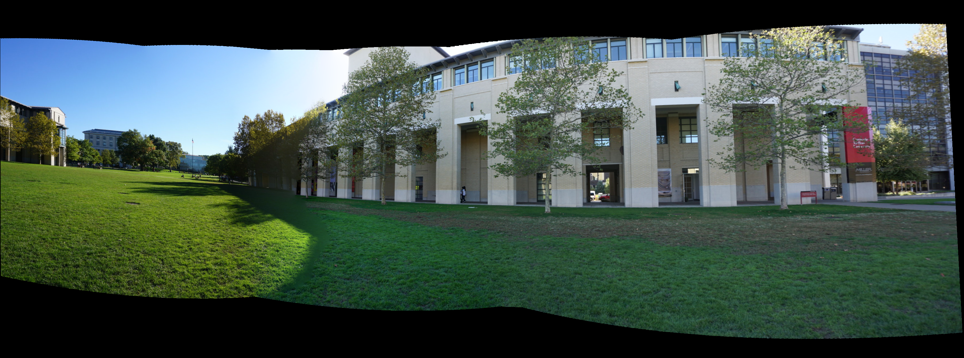
(b)

Figure 24: Stitched image with large number of images: Top: $6$ images from the CMU0 dataset [56]. Bottom: These images are aligned and stitched by BRAS accurately, which verifies its effectiveness in the case with a long sequence of images.

(a)

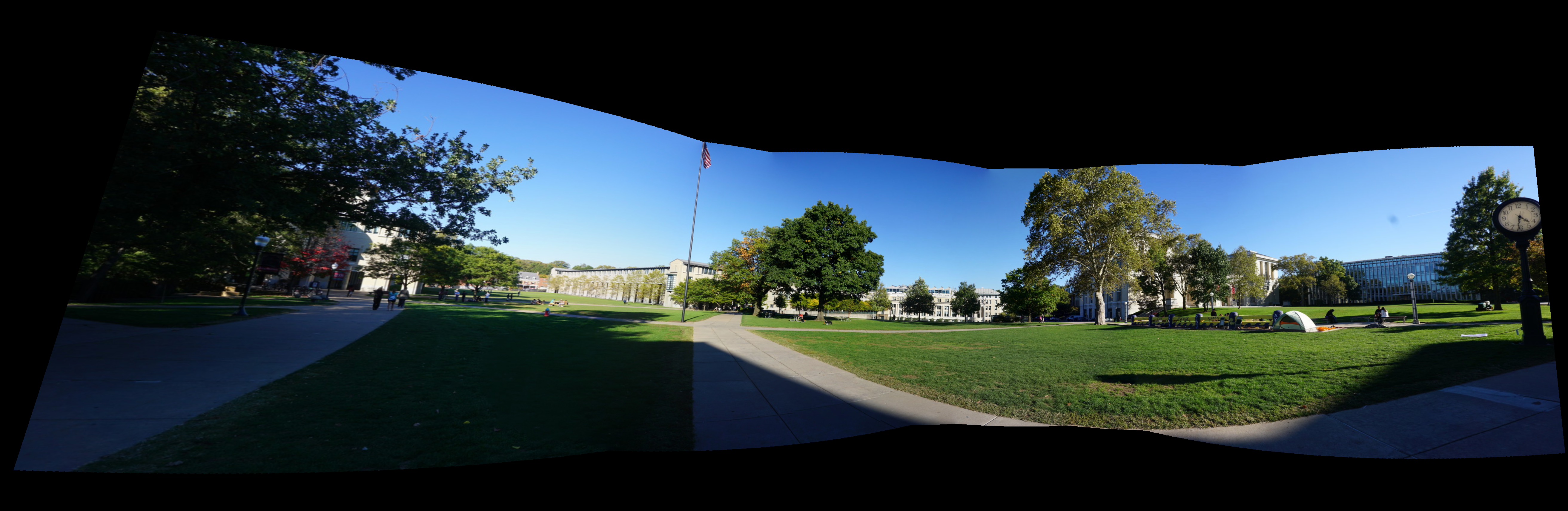
(b)

Figure 25: Stitched image with large number of images: Top: $6$ images from the CMU1 dataset [56]. Bottom: These images are aligned and stitched by BRAS accurately, which verifies its effectiveness in the case with a long sequence of images.

(a) AutoStitch [9]

(b) ICE [57]

(c) SPHP [21]

(d) APAP [12]

(e) BRAS

​  ​  ​  ​

Figure 26: Stitched images on the skyscraper dataset [21]. Regions with artifacts in some algorithms are magnified in boxes. Red circles in the insets highlight the artifacts.

(a) AutoStitch [9]

(b) ICE [57]

(c) SPHP [21]

(d) CPW [24]

(e) APAP [12]

(f) BRAS

Figure 27: Stitched images on the temple dataset [13]. Red circles in the insets highlight artifacts.

(a) AutoStitch [9]

(b) ICE [57]

(c) SPHP [21]

(d) APAP [12]

(e) BRAS

​  ​  ​  ​

Figure 28: Stitched images on the forest dataset [12]. Red circles in the insets highlight artifacts.

(a) AutoStitch [9]

(b) ICE [57]

(c) SPHP [21]

(d) APAP [12]

(e) BRAS

​  ​  ​  ​

Figure 29: Stitched images on the rooftops dataset [14]. Red circles in the insets highlight artifacts.

(a) AutoStitch [9]

(b) ICE [57]

(c) SPHP [21]

(d) CPW [24]

(e) APAP [12]

(f) BRAS

Figure 30: Stitched images on the carpark dataset [13]. Red circles in the insets highlight artifacts.

(a) AutoStitch [9]

(b) ICE [57]

(c) SPHP [21]

(d) CPW [24]

(e) APAP [12]

(f) BRAS

Figure 31: Stitched images on the couch dataset [13]. Red circles in the insets highlight artifacts.

(a)

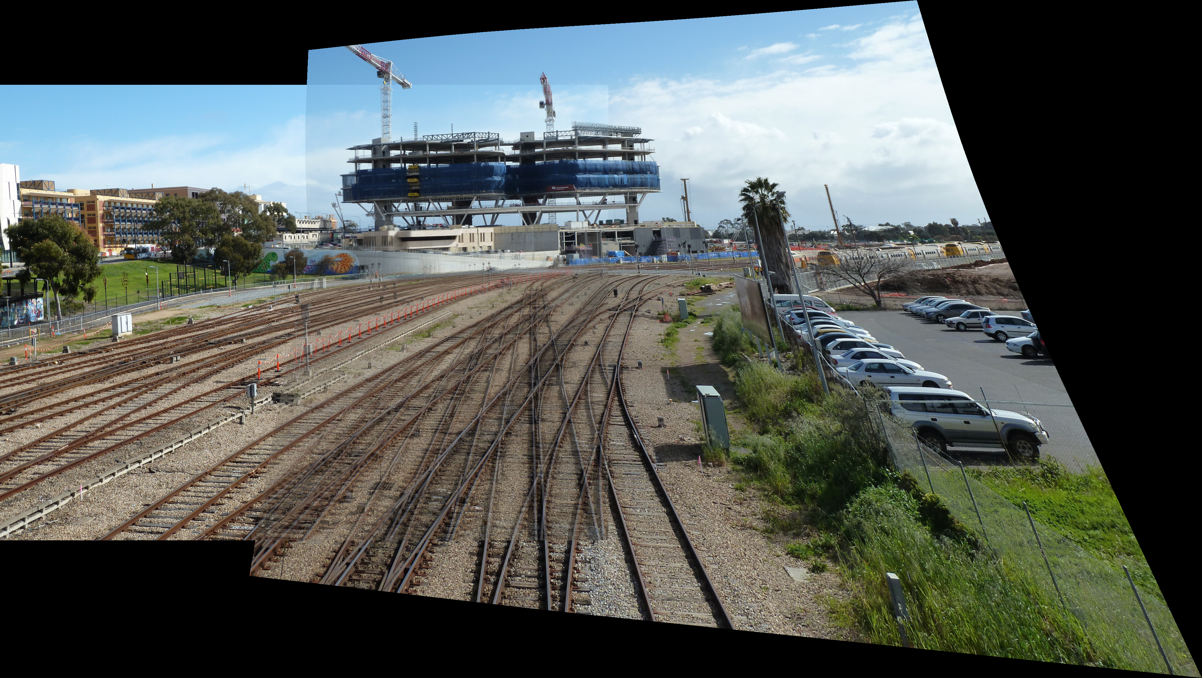
(b)

​

Figure 32: Comparison between LABEL:sub@subfig:bras_railtracks BRAS and LABEL:sub@subfig:multicell_railtracks a multi-cell extension to (12) on the railtracks image set. Note that the only difference between these two methods is on whether the rank-1 constraint is imposed and clearly the rank-1 constraint improves the alignment performance.

References

- [1] R. Szeliski, “Image alignment and stitching: A tutorial,” Found. Trends Comput. Graph. Vis., vol. 2, no. 1, pp. 1–104, 2006.
- [2] C. Liu, J. Yuen, and A. Torralba, “SIFT Flow: Dense Correspondence across Scenes and Its Applications,” IEEE Trans. Pattern Anal. Mach. Intell., vol. 33, no. 5, pp. 978–994, May 2011.
- [3] Y. Peng, A. Ganesh, J. Wright, W. Xu, and Y. Ma, “RASL: Robust alignment by sparse and low-rank decomposition for linearly correlated images,” IEEE Trans. Pattern Anal. Mach. Intell., vol. 34, no. 11, pp. 2233–2246, Nov. 2012.
- [4] R. Szeliski and H.-Y. Shum, “Creating Full View Panoramic Image Mosaics and Environment Maps,” in Proc. ACM SIGGRAPH, 1997.
- [5] A. Bartoli, “Groupwise Geometric and Photometric Direct Image Registration,” IEEE Trans. Pattern Anal. Mach. Intell., vol. 30, no. 12, pp. 2098–2108, Dec. 2008.
- [6] G. D. Evangelidis and E. Z. Psarakis, “Parametric Image Alignment Using Enhanced Correlation Coefficient Maximization,” IEEE Trans. Pattern Anal. Mach. Intell., vol. 30, no. 10, pp. 1858–1865, Oct. 2008.
- [7] V. Gay-Bellile, A. Bartoli, and P. Sayd, “Direct Estimation of Nonrigid Registrations with Image-Based Self-Occlusion Reasoning,” IEEE Trans. Pattern Anal. Mach. Intell., vol. 32, no. 1, pp. 87–104, Jan. 2010.
- [8] B. Triggs, P. F. McLauchlan, R. I. Hartley, and A. W. Fitzgibbon, “Bundle adjustment – a modern synthesis,” in Proc. IWVA, 1999.
- [9] M. Brown and D. G. Lowe, “Automatic Panoramic Image Stitching using Invariant Features,” Int. J. Comput. Vis., vol. 74, no. 1, pp. 59–73, Aug. 2007.
- [10] D. G. Lowe, “Distinctive Image Features from Scale-Invariant Keypoints,” Int. J. Comput. Vis., vol. 60, no. 2, pp. 91–110, Nov. 2004.
- [11] M. A. Fischler and R. C. Bolles, “Random Sample Consensus: A Paradigm for Model Fitting with Applications to Image Analysis and Automated Cartography,” Commun. ACM, vol. 24, no. 6, pp. 381–395, Jun. 1981.
- [12] J. Zaragoza, T. J. Chin, Q. H. Tran, M. S. Brown, and D. Suter, “As-Projective-As-Possible Image Stitching with Moving DLT,” IEEE Trans. Pattern Anal. Mach. Intell., vol. 36, no. 7, pp. 1285–1298, Jul. 2014.
- [13] J. Gao, S. J. Kim, and M. Brown, “Constructing image panoramas using dual-homography warping,” in Proc. IEEE CVPR, Jun. 2011.
- [14] W. Y. Lin, S. Liu, Y. Matsushita, T. T. Ng, and L. F. Cheong, “Smoothly varying affine stitching,” in Proc. IEEE CVPR, Jun. 2011.
- [15] J. Gao, Y. Li, T.-J. Chin, and M. S. Brown, “Seam-Driven Image Stitching.” in EG (Short Papers), 2013.
- [16] K. Lin, J. Nianjuan, L.-F. Cheong, D. Minh, and L. Jiangbo, “Seagull: Seam-guided local alignment for parallax-tolerant image stitching,” in Proc. ECCV, 2016.
- [17] F. Liu, M. Gleicher, H. Jin, and A. Agarwala, “Content-preserving warps for 3d video stabilization,” ACM Trans. Graph., vol. 28, no. 3, Jul. 2009.
- [18] F. Zhang and F. Liu, “Parallax-Tolerant Image Stitching,” in Proc. IEEE CVPR, Jun. 2014.
- [19] S. Li, L. Yuan, J. Sun, and L. Quan, “Dual-feature warping-based motion model estimation,” in Proc. IEEE ICCV, 2015, pp. 4283–4291.
- [20] K. Lin, N. Jiang, S. Liu, L.-F. Cheong, M. N. Do, and J. Lu, “Direct Photometric Alignment by Mesh Deformation.” in Proc. IEEE CVPR, 2017, pp. 2701–2709.
- [21] C. H. Chang, Y. Sato, and Y. Y. Chuang, “Shape-Preserving Half-Projective Warps for Image Stitching,” in Proc. IEEE CVPR, Jun. 2014.
- [22] N. Li, Y. Xu, and C. Wang, “Quasi-Homography Warps in Image Stitching,” IEEE Trans. Multimedia, vol. 20, no. 6, pp. 1365–1375, Jun. 2018.
- [23] C.-C. Lin, S. U. Pankanti, K. N. Ramamurthy, and A. Y. Aravkin, “Adaptive as-natural-as-possible image stitching,” in Proc. IEEE CVPR, 2015.
- [24] J. Hu, D.-Q. Zhang, H. Yu, and C. W. Chen, “Multi-objective content preserving warping for image stitching,” in Proc. IEEE ICME, 2015.
- [25] Y.-S. Chen and Y.-Y. Chuang, “Natural Image Stitching with the Global Similarity Prior,” in Proc. ECCV, 2016, pp. 186–201.
- [26] A. Agarwala, M. Agrawala, M. Cohen, D. Salesin, and R. Szeliski, “Photographing long scenes with multi-viewpoint panoramas,” ACM Trans. Graph., vol. 25, no. 3, pp. 853–861, Jul. 2006.
- [27] Qi Zhi and J. R. Cooperstock, “Toward Dynamic Image Mosaic Generation With Robustness to Parallax,” IEEE Trans. Image Process., vol. 21, no. 1, pp. 366–378, Jan. 2012.
- [28] G. Zhang, Y. He, W. Chen, J. Jia, and H. Bao, “Multi-Viewpoint Panorama Construction With Wide-Baseline Images,” IEEE Trans. Image Process., vol. 25, no. 7, pp. 3099–3111, Jul. 2016.
- [29] J. Li, Z. Wang, S. Lai, Y. Zhai, and M. Zhang, “Parallax-Tolerant Image Stitching Based on Robust Elastic Warping,” IEEE Trans. Multimedia, vol. 20, no. 7, pp. 1672–1687, Jul. 2018.
- [30] T.-Z. Xiang, G.-S. Xia, X. Bai, and L. Zhang, “Image stitching by line-guided local warping with global similarity constraint,” Pattern Recognition, vol. 83, pp. 481–497, Nov. 2018.
- [31] Y. Li and V. Monga, “SIASM: Sparsity-based image alignment and stitching method for robust image mosaicking,” in Proc. IEEE ICIP, 2016.
- [32] P. Jain, P. Netrapalli, and S. Sanghavi, “Low-rank matrix completion using alternating minimization,” in Proc. ACM STOC, 2013.
- [33] P. Netrapalli, N. U N, S. Sanghavi, A. Anandkumar, and P. Jain, “Non-convex Robust PCA,” in Adv. NIPS, 2014, pp. 1107–1115.
- [34] J. Wright, A. Ganesh, K. Min, and Y. Ma, “Compressive principal component pursuit,” Inf. Inference, 2013.
- [35] P. E. Debevec and J. Malik, “Recovering high dynamic range radiance maps from photographs,” in Proc. ACM SIGGRAPH, 1997.
- [36] C. Lee, Y. Li, and V. Monga, “Ghost-Free High Dynamic Range Imaging via Rank Minimization,” IEEE Signal Process. Lett., vol. 21, no. 9, pp. 1045–1049, Sep. 2014.
- [37] S. Baker and I. Matthews, “Lucas-Kanade 20 Years On: A Unifying Framework,” Int. J. Comput. Vis., vol. 56, no. 3, pp. 221–255, Feb. 2004.
- [38] J. Nocedal and S. Wright, Numerical optimization. Springer Science & Business Media, 2006.
- [39] J. Wright, A. Ganesh, S. Rao, Y. Peng, and Y. Ma, “Robust Principal Component Analysis: Exact Recovery of Corrupted Low-Rank Matrices via Convex Optimization,” in Adv. NIPS. Curran Associates, Inc., 2009, pp. 2080–2088.
- [40] E. J. Candès, X. Li, Y. Ma, and J. Wright, “Robust principal component analysis?” J. ACM, vol. 58, no. 3, p. 11, 2011.
- [41] B. Recht, M. Fazel, and P. Parrilo, “Guaranteed Minimum-Rank Solutions of Linear Matrix Equations via Nuclear Norm Minimization,” SIAM Rev., vol. 52, no. 3, pp. 471–501, Jan. 2010.
- [42] V. Chandrasekaran, S. Sanghavi, P. Parrilo, and A. Willsky, “Rank-Sparsity Incoherence for Matrix Decomposition,” SIAM J. Optim., vol. 21, no. 2, pp. 572–596, Apr. 2011.
- [43] M. Soltanolkotabi, E. Elhamifar, and E. J. Candès, “Robust subspace clustering,” Ann. Stat., vol. 42, no. 2, pp. 669–699, Apr. 2014.
- [44] G. H. Golub and C. F. Van Loan, Matrix Computations (3rd Ed.). Johns Hopkins University Press, 1996.
- [45] P. J. Huber, “Robust Estimation of a Location Parameter,” Ann. Math. Stat., vol. 35, no. 1, pp. 73–101, Mar. 1964.
- [46] C. M. Bishop, Pattern Recognition and Machine Learning (Information Science and Statistics). Secaucus, NJ, USA: Springer-Verlag New York, Inc., 2006.
- [47] P. F. Felzenszwalb and D. P. Huttenlocher, “Efficient Belief Propagation for Early Vision,” Int. J. Comput. Vis., vol. 70, no. 1, pp. 41–54, May 2006.
- [48] A. Agarwala, M. Dontcheva, M. Agrawala, S. Drucker, A. Colburn, B. Curless, D. Salesin, and M. Cohen, “Interactive digital photomontage,” ACM Trans. Graph., vol. 23, no. 3, pp. 294–302, Aug. 2004.
- [49] P. Pérez, M. Gangnet, and A. Blake, “Poisson image editing,” ACM Trans. Graph., vol. 22, pp. 313–318, 2003.
- [50] J. Brandt, “Transform coding for fast approximate nearest neighbor search in high dimensions,” in Proc. IEEE CVPR, Jun. 2010.
- [51] E. Ask, O. Enqvist, and F. Kahl, “Optimal Geometric Fitting under the Truncated L2-Norm,” in Proc. IEEE CVPR, Jun. 2013.
- [52] R. I. Hartley, “In defense of the eight-point algorithm,” IEEE Trans. Pattern Anal. Mach. Intell., vol. 19, no. 6, pp. 580–593, 1997.
- [53] Z. Zhou, X. Li, J. Wright, E. Candès, and Y. Ma, “Stable Principal Component Pursuit,” in Proc. ISIT, Jun. 2010.
- [54] “Hugin - Panorama Photo Stitcher,” http://hugin.sourceforge.net/.
- [55] W. Y. Lin, L. Liu, Y. Matsushita, K. L. Low, and S. Liu, “Aligning images in the wild,” in Proc. IEEE CVPR, Jun. 2012.
- [56] “OpenPano,” https://github.com/ppwwyyxx/OpenPano, accessed: 2019.
- [57] “Image Composite Editor (ICE),” https://www.microsoft.com/en-us/research/product/computational-photography-applications/image-composite-editor/.
- [58] “BRAS Webpage,” http://signal.ee.psu.edu/panorama.html.
- [59] R. Bhatia, Matrix Analysis, ser. Graduate Texts in Mathematics. New York, NY: Springer New York, 1997, vol. 169.