Accepted Manuscript - International Journal of Non-Linear Mechanics A study of temporary captures and collisions in the Circular Restricted Three-Body Problem with normalizations of the Levi-Civita Hamiltonian Captures and collisions in the CRTBP with normalizations of the Levi-Civita Hamiltonian Rocío I. Paez¹, Massimiliano Guzzo¹* celestial mechanics, captures, CR3BP The dynamics near the Lagrange equilibria $L_{1}$ and $L_{2}$ of the Circular Restricted Three-body Problem has gained attention in the last decades due to its relevance in some topics such as the temporary captures of comets and asteroids and the design of trajectories for space missions. In this paper we investigate the temporary captures using the tube manifolds of the horizontal Lyapunov orbits originating at $L_{1}$ and $L_{2}$ of the CR3BP at energy values which have not been considered so far. After showing that the radius of convergence of any Hamiltonian normalization at $L_{1}$ or $L_{2}$ computed with the Cartesian variables is limited in amplitude by $\left|1-\mu-x_{L_{1}}\right|$ ($\mu$ denoting the reduced mass of the problem), we investigate if regularizations allow us to overcome this limit. In particular, we consider the Hamiltonian describing the planar three-body problem in the Levi-Civita regularization and we compute its normalization for the Sun-Jupiter reduced mass for an interval of energy which overcomes the limit of Cartesian normalizations. As a result, for the largest values of the energy that we consider, we notice a transition in the structure of the tubes manifolds emanating from the Lyapunov orbit, which can contain orbits that collide with the secondary body before performing one full circulation around it. We discuss the relevance of this transition for temporary captures.

1 Introduction

In the last decades the close encounters of a small body with a planet have been investigated especially in connection with the dynamics of comets, of near-earth asteroids, and space mission design (see [1], [2], [3], [4], [5], [6], [7], [8], [9], [10], [11], [12], [13], [14], [15], [16], [17], [18], [19], [20], [21], [22], and references therein). A classical tool to classify a close encounter is given by the Tisserand parameter respect to a given planet,

$$T_{P}={a_{P}\over a}+2\sqrt{{a\over a_{P}}(1-e^{2})}\cos i$$

($a,e$ denote the semi-major axis and the eccentricity of the small body; $i$ denotes the inclination of the small body with respect to the orbit of the planet; $a_{P}$ denotes the semi-major axis of the planet) whose variation before and after each encounter is small. The Tisserand parameter gives a qualitative idea of the encounter: for increasing values of $T_{P}$ in a small interval around $T_{P}=3$, we have the transition between the ’fast’ encounters, occurring with an orbit of the small body which is hyperbolic in the planetocentric reference frame, and

©$<$2020$>$. This manuscript version is made available under the
CC-BY-NC-ND 4.0 license http://creativecommons.org/licenses/by-nc-nd/4.0/

the ’slow’ close encounters which can lead to a temporary capture of the small body. Öpik theory ([23], recently revisited in [24], [25]), provided good results in the study of the fast close encounters of comets with Jupiter and of near-Earth asteroids with the Earth ([26],[8]). The slow close encounters are instead better studied in the framework of the dynamics generating at the Lagrangian points $L_{1},L_{2}$ of the Circular Restricted Three–Body Problem, defined by the Hamiltonian

$$h={p_{x}^{2}+p_{y}^{2}+p_{z}^{2}\over 2}+p_{x}y-p_{y}x-{\mu\over\sqrt{(x-1+\mu)^{2}+y^{2}+z^{2}}}$$

$$-{1-\mu\over\sqrt{(x+\mu)^{2}+y^{2}+z^{2}}}\leavevmode\nobreak\ .$$ (1)

This Hamiltonian is written in the barycentric rotating reference frame and with the usual units of measure for this problem: the masses of the primaries $P_{1}$ and $P_{2}$ are $1-\mu$ and $\mu$ respectively; their coordinates are $(x_{1},0,0)=(-\mu,0,0)$, $(x_{2},0,0)=(1-\mu,0,0)$ and their revolution period is $2\pi$. The Hamiltonian $h$ and the Tisserand parameter are related by

$$T_{P}=-2h+{\cal O}(\mu)\leavevmode\nobreak\ .$$

For energy values $E>E_{1}$, where $E_{1}$ is the value of $h$ associated to the Lagrangian point $L_{1}$, the transits from the realm ${\cal S}$ of motions dominated by the Sun to the realm ${\cal P}$ of motions dominated by the planet (i.e. the temporary captures) and back, become possible (see [1], [27], [28], [22] for precise characterizations of the different realms of motion). Respectively for $E>E_{2}$, where $E_{2}$ is the value of $h$ associated to $L_{2}$, the transits from the realms ${\cal E}$ of motions which are external to the binary system to ${\cal P}$ (i.e. the temporary captures from the region external to the planet orbit) and back are possible. In the planar CR3BP (useful to study close encounters with small inclination), [1] has shown that the orbits which perform the transits are contained in two dimensional surfaces of the phase-space, the so-called tube manifolds of $L_{1}$ and $L_{2}$. These tube manifolds are defined as follows. Let us consider for definiteness the tube manifolds at $L_{1}$; for values of $E$ slightly larger than $E_{1}$ there is a periodic orbit of libration around $L_{1}$, the horizontal Lyapunov orbit denoted by $LL_{1}(E)$, whose amplitude increases rapidly as the value of $E$ increases. All the phase-space orbits which are asymptotic in the future (resp. in the past) to $LL_{1}(E)$ form a surface which, close to $LL_{1}(E)$, is topologically a 2-dimensional tube extending on both right and left sides of $LL_{1}(E)$ called the stable tube manifold $W^{s}_{1}(E)$ (resp. the unstable manifold $W^{u}_{1}(E)$) of $LL_{1}(E)$. Analogously, for $E$ slightly larger than $E_{2}$ we have the stable and unstable tube manifolds of $LL_{2}(E)$. The tube manifolds of $LL_{1}(E)$ separate the motions which transit between ${\cal S}$ and ${\cal P}$: for example, an orbit with $E>E_{1}$ which is a temporary satellite of the Sun, when it approaches the Lyapunov orbit $LL_{1}(E)$ transits to the realm ${\cal P}$ only if it is contained in the stable tube $W^{s}_{1}(E)$ of $LL_{1}(E)$, otherwise it bounces back to the realm ${\cal S}$. Therefore, numerical computations of the stable and unstable tube manifolds at various values of $E$ provide the relevant information to understand the transit properties related to the close encounters, e.g. to determine if a comet becomes a temporary satellite of Jupiter. A list of comets which have been identified as potential candidates for temporary captures can be found in [29]. For this reason, the Sun-Jupiter case, with mass ratio, $\mu=\mu_{J}:=9.537{\scriptstyle\times 10}^{[}-4]$, has received particular relevance in the literature (e.g. see [11], [21], [22]). Also in this paper we focus on $\mu=\mu_{J}$, while the methods that we use can be implemented with any other value. In particular, we correlate a property of the tube manifolds to a property of temporary captures which has been little considered in the literature: the number ${\cal N}$ of revolutions performed around Jupiter during the temporary capture and their orientation (clockwise or counter-clockwise) measured in the rotating reference frame. For simplicity, we consider the right-branch of the stable tube of the Lyapunov orbits $LL_{1}(E)$, and we identify three–situations:

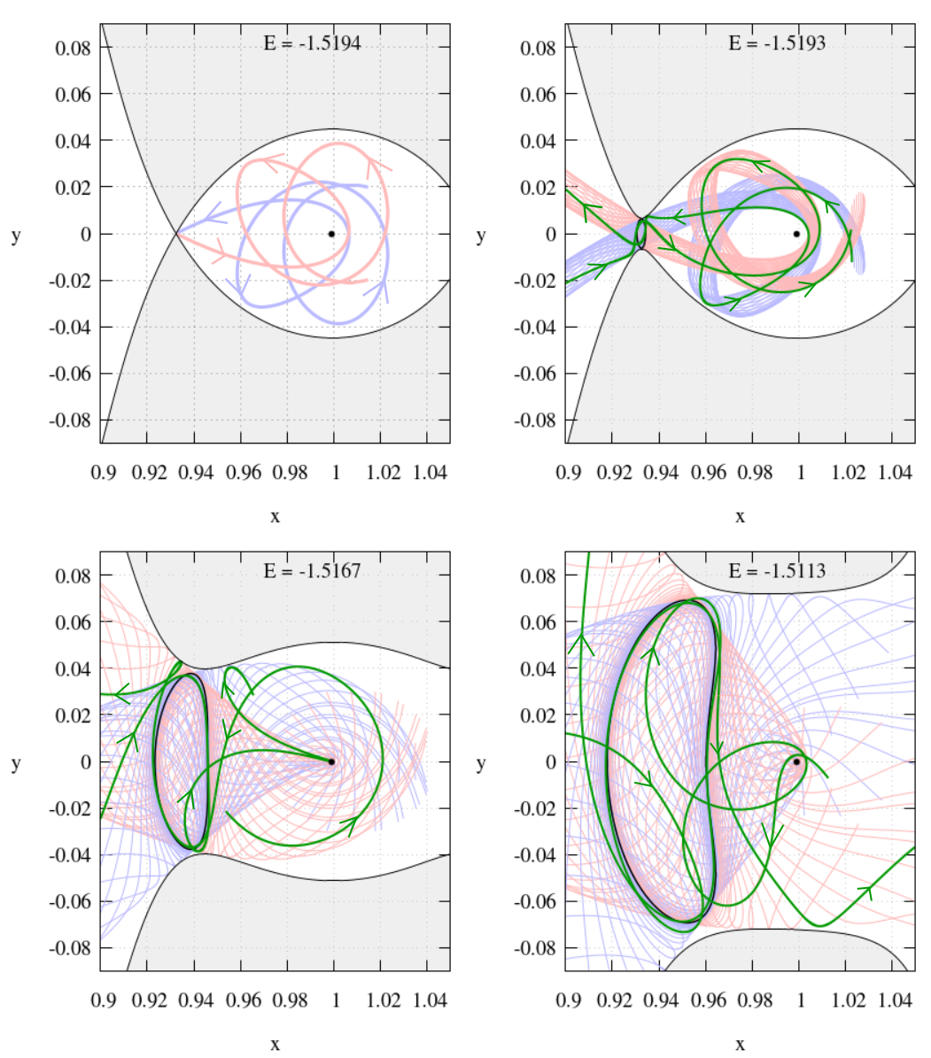
Figure 1: Lyapunov orbit $LL_{1}$ (black closed curves), stable tube manifold $W^{s}_{1}(C)$ (blue thin lines) and unstable tube manifold $W^{u}_{1}(C)$ (red thin lines), for four values of the energy, depicted in the plane $xy$ in a neighbourhood of the secondary body $P_{2}$. The shaded areas correspond to the regions of forbidden motion. Top left panel: $E=E_{1}\equiv-1.5194$ (see (i) in text); Top right panel: $E=-1.5194$, slightly larger than $E_{1}$ (see (ii) in text); Bottom panels: $E=-1.5167$ (left) and $E=-1.5113$ (right), values considerably larger than $E_{1}$ (see (iii) in text). In each case, the thick green lines corresponds to sample orbits from the manifolds, with the arrows indicating the sense of motion forward in time.

• for $E=E_{1}$, the tube collapses to only one limit orbit (see Fig. 1, top-left panel);

• for very small and positive values $E-E_{1}$, the numerical computation of the tube manifolds provides evidence that up to a fixed number ${\cal N}$ of revolutions all the orbits of the tube are not collision orbits, and perform the same number and type of revolutions
  around Jupiter as the limit orbit of (i). As a consequence, also the orbits in the interior of the tube share the same properties. In particular, since collisions are excluded within the ${\cal N}$ revolutions, all the orbits in the interior of the stable tube transit to the realm ${\cal S}$ after the ${\cal N}$ revolutions (see Fig. 1, top-right panel, for ${\cal N}=2$).

• The question is what happens for increasing values of $E-E_{1}$, which corresponds to increasing amplitudes of the stable/unstable tubes. When these amplitude are large, we find that the tube manifolds become so large and stretched in phase-space that the criterion of using them as separatrices for the transit properties is no more as effective as when their amplitude is small. In this paper we propose a threshold on $E$ based on the appearance of peculiar orbits in the stable tube. This orbit originates from a collision with Jupiter and converges to the Lyapunov orbit $LL_{1}(E)$ before performing a full revolution around the planet. In addition to this peculiar orbit, we find that the stable tube contains also orbits performing either clockwise or counter-clockwise revolutions (see Fig. 1, bottom panels). The same properties are shared by the orbits in the interior of the tube. In particular, due to possible collisions, it is no more granted that all the orbits in the interior of the tube will transit to the realm ${\cal S}$.

The conclusions outlined above have been obtained thanks to a method of computation of the tube manifolds which exploits the well known Levi-Civita regularization of the three-body problem and the method of normalization of an Hamiltonian at a partially hyperbolic equilibrium. The combination of the two techniques allows us to reach values of the energy never investigated before.

There are several methods for computing numerically the stable and unstable manifolds of periodic orbits, such as the flow continuation of the local manifolds, the parametrization method, and the recent method based on chaos indicators. In the first two the manifolds are developed from analytic approximations of the local stable and unstable manifolds (see for example [30]), in the latter the manifolds are obtained as the ridges of a chaos indicator defined from a Hamiltonian normalization ([17], [21], [22]). We remark that Hamiltonian normalizations provide not only high precision computations of the local stable/unstable manifolds, but also of all the orbits in their neighbourhood, suitable for astronomical applications. For this reason, in this paper we push the method of Hamiltonian normalization to its limit, by implementing it in the Levi-Civita regularization of the CR3BP.

Even if the Hamiltonian normalization method has been extensively used to compute the tube manifolds, its limits have to be improved, especially if one aims to extend its application to a broader interval of energies. In the present work, we show that the use of the Levi-Civita regularization is necessary in order to normalize the Hamiltonian at values of the energy for which we detect the transition from situation (ii) to (iii) described above.

In Section 2 we describe all the steps necessary to perform the normalization of the Levi-Civita Hamiltonian. In particular, we find that for $E>E_{1}$ the regularized Hamiltonian still has an equilibrium, not corresponding to an orbit of the CR3BP. Nevertheless the Levi-Civita Hamiltonian can be normalized at these ’fictitious’ equilibria, providing the Lyapunov orbit as well as their stable and unstable manifolds. In Section 3 we discuss the efficiency of the normal form computations of $L_{1}$. In Section 4, we show the computations of the manifolds via the normalized Levi-Civita Hamiltonian, for a wide range of energies such that the amplitude of the corresponding Lyapunov orbit is larger than $\left|1-\mu-x_{L_{1}}\right|$. While for small $E$ the stable tube manifold ${W}^{s}_{1}(E)$ folds around $P_{2}$ exclusively in a clockwise fashion (when integrated backwards in time for ${\cal N}=2$), for large values of $E$ the folding can be either clockwise or counter-clockwise. It is within this range of energy values where we identify the transition between the orbits discussed at ii) and iii).

2 Hamiltonian normalizations

Powerful methods to analyze the dynamics originating at the Lagrangian points $L_{1},L_{2}$ of the CR3BP rely on the Birkhoff normalizations of the Hamiltonian with a large normalization order $N$ ([7], [4], [31]). For the planar problem, this implies the explicit construction, for any value of an integer parameter $N\geq 3$, of a canonical transformation

$$(x,y,p_{x},p_{y})=C_{N}(Q_{1},Q_{2},P_{1},P_{2})$$ (2)

conjugating the Hamiltonian of the planar circular restricted three–body problem

$$h= {p_{x}^{2}+p_{y}^{2}\over 2}+p_{x}y-p_{y}x-{\mu\over\sqrt{(x-1+\mu)^{2}+y^{2}}}$$ (3)

$$-{1-\mu\over\sqrt{(x+\mu)^{2}+y^{2}}}$$

to a normal form Hamiltonian

$$H={E}_{i}+\sum_{j=2}^{N}K_{j}(Q_{1},Q_{2},P_{1},P_{2})+\sum_{j\geq N+1}{\cal R}_{j}(Q_{1},Q_{2},P_{1},P_{2})\leavevmode\nobreak\ .$$ (4)

The Hamiltonian in (4) is analytic in some neighbourhood of the Lagrange equilibrium $L_{i}$, represented by $(Q,P)=(0,0,0,0)$ (the radius of the neighborhood depending on the mass ratio $\mu$ and $N$), $K_{j},{\cal R}_{j}$ are polynomials in $P,Q$ of order $j$, the polynomials $K_{j}$ depend on the $Q_{1},P_{1}$ only through the product $Q_{1}P_{1}$ and

$$K_{2}=\lambda Q_{1}P_{1}+\omega\,{P_{2}^{2}+Q_{2}^{2}\over 2}\leavevmode\nobreak\ ,$$ (5)

(alternative reduction methods can be considered, see Section 3 for details). By neglecting the remainder terms ${\cal R}_{j}$ we obtain

• The approximated equations of the Lyapunov orbits labeled by $E$

  $${LL}_{i}(E)=\Big{\{}Q,P:\ \ Q_{1},P_{1}=0,\ \ E_{i}+\sum_{j=2}^{N}{K}_{j}(0,Q_{2},0,P_{2})=E\Big{\}}\leavevmode\nobreak\ ,$$ (6)

• the approximated equations of the (local) stable and unstable manifolds of ${LL}_{i}(E)$

  $${W}^{s}_{i}(E)=\Big{\{}Q,P:\ \ Q_{1}=0,\ \ E_{i}+\sum_{j=2}^{N}{K}_{j}(0,Q_{2},P_{1},P_{2})=E\Big{\}},$$

  $${W}^{u}_{i}(E)=\Big{\{}Q,P:\ \ P_{1}=0,\ \ E_{i}+\sum_{j=2}^{N}{\cal K}_{j}(Q_{1},Q_{2},0,P_{2})=E\Big{\}},$$

• the arcs of approximated orbits in a neighbourhood of ${W}^{s}_{i}(E)$, ${W}^{u}_{i}(E)$ which are scattered by $LL_{i}(E)$.

For increasing values of $E$, the periodic orbit ${LL}_{i}(E)$ has increasing libration amplitude. As a consequence, for suitably large values of $E$, we expect a breakdown of the method. A natural limit for this breakdown is given by the singularity in the gravitational potential energy at the position of $P_{2}$ which, for small values of $\mu$, is close to $L_{1},L_{2}$. Since the Lyapunov orbits ${LL}_{i}(E)$ are typically larger in the $y$ coordinate with respect to the $x$ coordinate, a dangerous complex singularity is the one located at $x=x_{L_{j}}$ and $y=\pm i\left|1-\mu-x_{L_{j}}\right|$ (for $\mu=\mu_{J}$, $y=\pm i0.066...$). This singularity severely limits the validity of these methods for libration amplitudes in the $y$ variable of order of $\left|1-\mu-x_{L_{j}}\right|$. We here investigate the possibility to overcome this limit by implementing the normalization methods using the Levi-Civita regularization ([32]) on the secondary body $P_{2}$. Similar approaches has been used in the past for the simpler Hill’s problem, e.g. [33].

Following [32], we first perform the phase-space translation

$$X=x-x_{2}\leavevmode\nobreak\ ,\quad Y=y\leavevmode\nobreak\ ,\quad P_{X}=p_{x}\leavevmode\nobreak\ ,\quad P_{Y}=p_{y}-x_{2}\leavevmode\nobreak\ \leavevmode\nobreak\ ,$$ (7)

on Hamiltonian (3), and then we introduce the Levi-Civita variables $(u_{1},u_{2})$ canonically extended to the momenta $(U_{1},U_{2})$

$$X=u_{1}^{2}-u_{2}^{2}\leavevmode\nobreak\ ,Y=2u_{1}u_{2}\leavevmode\nobreak\ ,$$ (8)

$$\text{\normalsize$P_{X}=\frac{U_{1}u_{1}-U_{2}u_{2}}{2|u|^{2}}$}\leavevmode\nobreak\ ,\text{\normalsize$P_{Y}=\frac{U_{1}u_{2}+U_{2}u_{1}}{2|u|^{2}}$}\leavevmode\nobreak\ ,$$

and the fictitious time $\tau$

$$dt=|u|^{2}d\tau$$ (9)

where $|{u}|^{2}=u_{1}^{2}+u_{2}^{2}=\sqrt{(x-1+\mu)^{2}+y^{2}}$. For any fixed value of $E$ of the Hamiltonian (3), we define the Levi-Civita Hamiltonian

$${\cal K}_{E}(u,U)=$$ (10)

$$=\left|{u}\right|^{2}\left[h\Big{(}X(u)+x_{2},Y(u),P_{X}(u,U),P_{Y}(u,U)+x_{2}\Big{)}-E\right]$$

$$=\left|{u}\right|^{2}\left[h\left(\text{\small$u_{1}^{2}-u_{2}^{2}+x_{2}$},\text{\small$2u_{1}u_{2}$},\text{\footnotesize$\frac{U_{1}u_{1}-U_{2}u_{2}}{2|u|^{2}}$},\text{\footnotesize$\frac{U_{1}u_{2}+U_{2}u_{1}}{2|u|^{2}+x_{2}}$}\right)-E\right]$$

$$=\frac{1}{8}\left(U_{1}+2\left|{u}\right|^{2}u_{2}\right)^{2}+\frac{1}{8}\left(U_{2}-2\left|{u}\right|^{2}u_{1}\right)^{2}$$

$$-\frac{1}{2}\left|{u}\right|^{6}-\mu-|{u}|^{2}\left(E+\frac{(1-\mu)^{2}}{2}\right)$$

$$-(1-\mu)|{u}|^{2}\left[\frac{1}{\sqrt{1+2(u_{1}^{2}-u_{2}^{2})+|{u}|^{4}}}+u_{1}^{2}-u_{2}^{2}\right]\leavevmode\nobreak\ ,$$

which is a regularization of the planar three-body problem at $P_{2}$. In fact, ${\cal K}_{E}$ is regular at $u=(0,0)$ which correspons to a collision with $P_{2}$. The solutions $({u}(\tau),{U}(\tau))$ of the Hamilton equations of ${\cal K}_{E}$,

$${du_{j}\over d\tau}={\partial\over\partial U_{j}}{\cal K}_{E}(u,U)\ \ ,\ \ {dU_{j}\over d\tau}=-{\partial\over\partial u_{j}}{\cal K}_{E}(u,U)$$ (11)

with initial conditions satisfying ${u}(0)\neq 0$ and
${\cal K}_{E}({u}(0),{U}(0))=0$, are conjugate, in a neighbourhood of $\tau=0$, via Eq. (8) and

$$t=\int_{0}^{\tau}\left|u(s)\right|^{2}ds,$$

to solutions $(X(t),Y(t),P_{X}(t),P_{Y}(t))$ of the three-body problem Hamiltonian (see [34]). For definiteness, we describe the normalization of the Levi-Civita Hamiltonian at the Lagrangian point $L_{1}$; a similar method applies to $L_{2}$. Equilibrium points of ${\cal K}_{E}$. The regularized Hamiltonian ${\cal K}_{E}$, for increasing values of $E\geq E_{1}$, has a family of equilibria continued from $L_{1}$. Since the equilibria of the family are characterized by $u_{1},U_{2}=0$ and $U_{1}=-2u_{2}^{3}$, we define the fictitious equilibrium position as

$$(u_{*},U_{*}):=(0,u_{2_{*}}^{\phantom{3}}\!\,,-2\left(u_{2_{*}}^{\phantom{3}}\!\right)^{3},0)\leavevmode\nobreak\ ,$$ (12)

where $u_{2_{*}}^{\phantom{3}}\!:=u_{2_{*}}^{\phantom{3}}\!(E)$ solves the algebraic equation
$F(u_{2_{*}}^{\phantom{3}}\!(E),E)=0$ with

$$F( u_{2_{*}}^{\phantom{3}}\!,E)=-2\left(E+\frac{1}{2}(1-\mu)^{2}\right)-3(u_{2_{*}}^{\phantom{3}}\!)^{4}$$ (13)

$$+(1-\mu)\left(4(u_{2_{*}}^{\phantom{3}}\!)^{2}-{2(u_{2_{*}}^{\phantom{3}}\!)^{2}\over(1-(u_{2_{*}}^{\phantom{3}}\!)^{2})^{2}}-{2\over 1-(u_{2_{*}}^{\phantom{3}}\!)^{2}}\right)\leavevmode\nobreak\ .$$

In Appendix 1 (see paragraphs A1 and A2) we prove that equation $F(u_{*,2},E)=0$ has a unique solution $u_{2_{*}}^{\phantom{3}}\!$ for all the values of $E$ in an interval $E\in[E_{1},E_{*}]$ where

$$E_{*}=-{3\over 2}\left(1-{4\over 3}\mu+{1\over 3}\mu^{2}\right).$$ (14)

The critical value (14) appears in the study of close encounters with $P_{2}$ as a threshold value for considering a close encounters fast or slow (see, for example, Section 3.1 of [15]). With this classification we are considering the regime of slow close encounters. The function $u_{2_{*}}^{\phantom{3}}\!(E)$ is strictly monotone increasing, and the extremal values range from $u_{2_{*}}^{\phantom{3}}\!(E_{1})=-\sqrt{1-\mu-x_{L_{1}}}$ (so that $(u_{1},u_{2})=(0,u_{2_{*}}^{\phantom{3}}\!(E_{1}))$ corresponds to the equilibrium $L_{1}$) to $u_{2_{*}}^{\phantom{3}}\!(E_{*})=0$ (so that $(u_{1},u_{2})=(0,0)$ is the collision point). Except for $E=E_{1}$, we have ${\cal K}_{E}(u_{*},U_{*})\neq 0$, therefore $(u_{*},U_{*})$ does not correspond to a solution of the three–body problem (no equilibria of the CR3BP different from $L_{1}$ exist for $y=0$ and $x\in(-\mu,1-\mu)$). Nevertheless the equilibrium $(u_{*},U_{*})$ can be used to perform a Birkhoff normalization of the Levi-Civita Hamiltonian (10). We remark that for small values of $\mu$ the energy interval $(E_{1},E_{*})$ seems small (for instance, for $\mu=\mu_{J}$, $(E_{1},E_{*})\sim(-1.5193,-1.49809)$) but tiny variations of the energy in this interval produce large variations in the amplitude of the Lyapunov orbits.

In Appendix 1, paragraph A3, we show that for any $\mu\in(0,1/2)$, and any $E\in(E_{1},E_{*})$ the fictitious equilibria $(u_{*},U_{*})$ are of saddle-center type, with two imaginary eigenvalues $\pm i\omega$ and two real eigenvalues $\pm\lambda$, with $\lambda,\omega>0$. Moreover, for $a$ going to zero, both $\lambda,\omega$ tend to zero as $(u_{2_{*}}^{\phantom{3}}\!)^{2}$.

The quadratic part of ${\cal K}_{E}$ expanded at $(u_{*},U_{*})$. For all $E\in(E_{1},E_{*})$, the Levi-Civita Hamiltonian ${\cal K}_{E}$ has a saddle-center equilibrium in $(u_{*},U_{*})$ and, as indicated in Appendix 1 paragraph A4, one can construct a canonical change of variables

$$(u_{1},u_{2},U_{1},U_{2})=A\ (\xi,q,\eta,p)+(u_{*,1},u_{*,2},U_{*,1},U_{*,2})$$ (15)

conjugating ${\cal K}_{E}(u,U)$ to the Hamiltonian

$${\cal K}^{(2)}_{E}(\xi,q,\eta,p)=K_{0}+K_{2}(\xi,q,\eta,p)+\sum_{j\geq 3}k_{j}(\xi,q,\eta,p)\leavevmode\nobreak\ ,$$ (16)

where $K_{0}={\cal K}_{E}(u_{*},U_{*})$,

$$K_{2}=\lambda\,\xi\,\eta+i\omega\,q\,p\leavevmode\nobreak\ ,$$ (17)

and $k_{j}(\xi,\eta,q,p)$ are homogeneous polynomials of degree $j$ expressed as sum of monomials of the type

$$\alpha^{(2)}_{k_{1},\,l_{1},\,k_{2},\,l_{2}}\,q^{k_{1}}\,p^{l_{1}}\,\xi^{k_{2}}\,\eta^{l_{2}}\ .$$ (18)

Note that the couple of conjugate variables $\xi,\eta$ is related to the hyperbolic behaviour, while the couple of conjugate variables $q,p$ is related to the elliptic behaviour (moreover, $q,p\in{\mathbb{C}}$ but, for real values of $u,U$, they satisfy $q=-ip$). The Hamiltonian in Eq. (16) is the starting point for the algorithm performing the Birkhoff normalization.

Normal forms of the Levi-Civita Hamiltonian at $L_{1}$. We reproduce with the Levi-Civita Hamiltonian the normalization methods which have been introduced in the Cartesian variables ([4], [31]). We perform a normal form scheme that uncouples (up to any arbitrary order) the hyperbolic variables $\xi,\eta$ from the elliptic variables $q,p$. The normalization is a near to the identity canonical transformation ${\cal C}_{N}$ which conjugates the Hamiltonian (16) to the normal form Hamiltonian

$${\cal K}^{(N)}_{E} ={\cal K}^{(2)}_{E}({\cal C}_{N}(\xi,q,\eta,p))$$ (19)

$$=K_{0}+\lambda\,\xi\,\eta+i\omega\,q\,p+\sum_{j=3}^{N}K_{j}(\xi,q,\eta,p)$$

$$+\sum_{j\geq N+1}{\cal R}^{(N)}_{j}(\xi,q,\eta,p),$$

where $N\geq 3$ is an integer called normalization order, ${\cal R}^{(N)}_{j}$ are polynomials of order $j$ expressed as sum of monomials of the type:

$$\alpha^{(N)}_{k_{1},\,l_{1},\,k_{2},\,l_{2}}\,q^{k_{1}}\,p^{l_{1}}\,\xi^{k_{2}}\,\eta^{l_{2}}\ ,$$ (20)

while the $K_{j}$ are polynomials of order $j$ having a specific form defined by a certain strategy (see [35], [36] for an introduction to polynomial normal forms). A traditional strategy is to require that all the $K_{j}$ commute with $K_{2}$. For motivations specific of the three-body problem, such as the optimization of the computational time (which is crucial to perform a large number $N\geq 20$ of normalizations) and due to the bifurcations occurring in the spatial case preventing the integrability on the center manifold, the reduction is usually performed with a weaker normal form. In this paper, for the sake of comparison, we consider the three strategies:

• the $K_{j}$ depend on the variables $\xi$, $\eta$ only through the product $\xi\eta$ (i.e. the canonical transformation eliminates from the normal form every monomial of order smaller or equal than $N$ for which $k_{2}\neq l_{2}$, see [4]). As a consequence, by neglecting the terms ${\cal R}_{j}$ (which are of order $j\geq N+1$), from the normal form Hamiltonian ${\cal K}^{(N)}_{E}$, we obtain an approximate normal form of type

  $$K^{(N)}_{E}:=K_{0}+\lambda\,\xi\,\eta+i\omega\,q\,p+{\cal J}(\xi\eta,q,p)$$ (21)

  where ${\cal J}$ is polynomial. From (21) one computes the center manifold (corresponding to $\xi,\eta=0$) as well as its stable (corresponding to $\xi=0,\eta\neq 0$) and unstable (corresponding to $\eta=0,\xi\neq 0$) manifolds.

• the $K_{j}$ contain only two type of monomials (18): monomials independent of $\xi,\eta$ and dependent on the $q,p$ only through the product $qp$, as well as monomials at least quadratic in $\xi,\eta$ (i.e. the canonical transformation eliminates every monomial for which $k_{2}+l_{2}=1$, or those which simultaneously satisfy that $k_{2}+l_{2}=0$ and $k_{1}\neq l_{1}$, see [31]). Neglecting the polynomials ${\cal R}_{j}$, we obtain an approximate normal form of type

  $$K^{(N)}_{E}: =K_{0}+\lambda\,\xi\,\eta+i\omega\,q\,p+{\cal J}_{0}(qp)$$ (22)

  $$+\xi^{2}\,{\cal J}_{1}(\xi,q,\eta,p)+\eta^{2}\,{\cal J}_{2}(\xi,q,\eta,p)$$

  $$+\xi\,\eta\,{\cal J}_{3}(\xi,q,\eta,p)$$

  where ${\cal J}_{0},\ldots,{\cal J}_{3}$ are polynomial functions. From (22) one computes the center manifold (corresponding to $\xi,\eta=0$), but not its stable and unstable manifolds.

• the $K_{j}$ contain only two type of monomials (18): monomials independent of $\xi,\eta$ and monomials at least quadratic in $\xi,\eta$ (i.e. the canonical transformation eliminates every monomial for which $k_{2}+l_{2}=1$, to our knowledge this strategy has been never introduced before). Neglecting the polynomials ${\cal R}_{j}$, we obtain an approximate normal form of type

  $$K^{(N)}_{E}: =K_{0}+\lambda\,\xi\,\eta+i\omega\,q\,p+{\cal J}_{0}(q,p)$$ (23)

  $$+\xi^{2}{\cal J}_{1}(\xi,q,\eta,p)+\eta^{2}{\cal J}_{2}(\xi,q,\eta,p)$$

  $$+\xi\eta{\cal J}_{3}(\xi,q,\eta,p)$$

  where ${\cal J}_{0},\ldots,{\cal J}_{3}$ are polynomial functions. From (23) one computes the center manifold (corresponding to $\xi,\eta=0$), but not its stable and unstable manifolds.

While all these strategies allow one to compute the center manifolds, only strategy (a) allows one to compute also its stable and unstable manifolds. On the other hand, for any given normalization order $N$, the normal form (a) has less monomial terms than the normal form (b), which in turn has less monomial terms than the normal form (c). Thus, the computation of the normal form (a) requires the elimination of a larger number of monomials, and is heavier than the computation of the normal form (b) or (c). Therefore, if one is interested only in the computation of the Lyapunov orbits, then the best strategy is to adhere to the procedure that requires the minimum amount of eliminations, i.e. (b) or (c). On the other hand, if one is interested also in the computation of the stable and unstable manifolds $W^{s}_{1}(E),W^{u}_{1}(E)$, and the dynamics in their neighbourhood, then one adheres to the procedure (a).

Algorithm for the construction of the normal forms. For each $N\geq 3$, the canonical transformation ${\cal C}_{N}$ conjugating the Hamiltonian (16) to the normal form Hamiltonian (19) is obtained from the composition of canonical transformations:

$${\cal C}_{N}={\cal C}_{\chi_{N}}\,\circ\,{\cal C}_{N-1}\leavevmode\nobreak\ ,$$ (24)

where ${\cal C}_{\chi_{N}}$ is the Hamiltonian flow at time $t=1$ of a suitable generating function defined from the coefficients of ${\cal K}^{(N-1)}_{E}$, and ${\cal C}_{2}$ is the identity. Below we describe the steps required for the computation of each ${\cal C}_{N}$ and ${\cal K}^{(N)}_{E}$ using the Lie series method (for an introduction to the method, see [37], [38]). We assume that the normal form ${\cal K}^{(N-1)}_{E}$ and ${\cal C}_{N-1}$ are known.

Step 1: From ${\cal K}^{(N-1)}_{E}$, we compute the generating function ${\chi_{N}}$, according to the chosen strategy:

– For strategy (a)

$$\chi_{N}=\sum_{\begin{subarray}{c}{k},{l}\in{\mathbb{N}}^{2}:\\ \sum_{n}(k_{n}+l_{n})=N,\\ k_{2}\neq l_{2}\end{subarray}}{-\alpha^{(N-1)}_{k_{1},l_{1},k_{2},l_{2}}\over i\omega(l_{1}-k_{1})+\lambda(l_{2}-k_{2})}\,q^{k_{1}}\,p^{l_{1}}\,\xi^{k_{2}}\,\eta^{l_{2}}\leavevmode\nobreak\ .$$ (25)

– For strategy (b)

$$\chi_{N}=\sum_{\begin{subarray}{c}{k},{l}\in{\mathbb{N}}^{2}:\\ \sum_{n}(k_{n}+l_{n})=N,\\ k_{2}+l_{2}=1\,\lor\\ k_{2}+l_{2}=0\,\land\,k_{1}\neq l_{1}\end{subarray}}{-\alpha^{(N-1)}_{k_{1},l_{1},k_{2},l_{2}}\over i\omega(l_{1}-k_{1})+\lambda(l_{2}-k_{2})}\,q^{k_{1}}\,p^{l_{1}}\,\xi^{k_{2}}\,\eta^{l_{2}}\leavevmode\nobreak\ .$$ (26)

– For strategy (c)

$$\chi_{N}=\sum_{\begin{subarray}{c}{k},{l}\in{\mathbb{N}}^{2}:\\ \sum_{n}(k_{n}+l_{n})=N,\\ k_{2}+l_{2}=1\end{subarray}}{-\alpha^{(N-1)}_{k_{1},l_{1},k_{2},l_{2}}\over i\omega(l_{1}-k_{1})+\lambda(l_{2}-k_{2})}\,q^{k_{1}}\,p^{l_{1}}\,\xi^{k_{2}}\,\eta^{l_{2}}\leavevmode\nobreak\ .$$ (27)

Step 2: We compute the canonical transformation

$${\cal C}_{\chi_{N}}(\tilde{\xi},\tilde{q},\tilde{\eta},\tilde{p})=(\xi,q,\eta,p)$$

defined by the Hamiltonian flow at time $t=1$ of $\chi_{N}$ as the Lie series

$$\zeta=e^{\,L_{\chi_{N}}}\tilde{\zeta}:=\tilde{\zeta}+\{\tilde{\zeta},\chi_{N}\}+{1\over 2}\{\{\tilde{\zeta},\chi_{N}\},\chi_{N}\}+\ldots\leavevmode\nobreak\ ,$$ (28)

where $L_{\chi_{N}}\equiv\{\cdot,\chi_{N}\}$ is the Poisson bracket operator and $\zeta,\tilde{\zeta}$ denote any of the variables $\xi,q,\eta,p$ and $\tilde{\xi},\tilde{q},\tilde{\eta},\tilde{p}$ respectively.

Step 3: We compute the transformed Hamiltonian

$${\cal K}^{(N)}_{E}={\cal C}_{\chi_{N}}\,{\cal K}^{(N-1)}_{E}=e^{L_{\chi_{N}}}\,{\cal K}^{(N-1)}_{E}$$ (29)

which, by construction, is in normal form up to order $N$, i.e. as in Eq. (19).

In summary, for any given $N$ we obtain the transformation yielding the original variables $(\xi,q,\eta,p)$ in terms of the normalized variables $(\xi^{(N)},q^{(N)},\eta^{(N)},p^{(N)})$, via

$$(\xi,q,\eta,p) ={\cal C}_{N}\,(\xi^{(N)},q^{(N)},\eta^{(N)},p^{(N)})$$

$$=e^{L_{\chi_{N}}}\,\ldots e^{L_{\chi_{3}}}\,(\xi^{(N)},q^{(N)},\eta^{(N)},p^{(N)})\leavevmode\nobreak\ .$$

The inverse transformation, i.e. the transformation yielding the normalized variables in terms of the original variables, is given by

$$(\xi^{(N)},q^{(N)},\eta^{(N)},p^{(N)})=e^{-L_{\chi_{3}}}\,\ldots e^{-L_{\chi_{N}}}\,(\xi,q,\eta,p)\leavevmode\nobreak\ .$$ (30)

Solutions of Hamilton equations of the normal form Hamiltonian. Let us consider the solutions ($\xi^{(N)}(\tau)$,$q^{(N)}(\tau)$,
$\eta^{(N)}(\tau)$,$p^{(N)}(\tau)$) of the Hamilton’s equations of (19),

$${d\xi^{(N)}\over d\tau}={\partial{\cal K}_{E}^{(N)}\over\partial\eta^{(N)}}\ \ ,\ \ {d\eta^{(N)}\over d\tau}=-{\partial{\cal K}_{E}^{(N)}\over\partial\xi^{(N)}}$$

$${dq^{(N)}\over d\tau}={\partial{\cal K}_{E}^{(N)}\over\partial p^{(N)}}\ \ ,\ \ {dp^{(N)}\over d\tau}=-{\partial{\cal K}_{E}^{(N)}\over\partial q^{(N)}}$$

on the zero-energy level of ${\cal K}_{E}^{(N)}$, transformed back to the variables $u,U$ using the transformations (15) and (30),

$$(\xi,q,\eta,p) =\left({\cal C}_{N}(\xi^{(N)},q^{(N)},\eta^{(N)},p^{(N)}\right)$$

$$(u_{1},u_{2},U_{1},U_{2}) =A(\xi,q,\eta,p)+(u_{*,1},u_{*,2},U_{*,1},U_{*,2})\leavevmode\nobreak\ .$$

They project to solutions of the three-body problem of energy $E$ via the Levi-Civita transformation. In fact, since the transformations (15) and (30) are canonical, we only have to prove that, for any initial condition ($\xi^{(N)}(0)$,$q^{(N)}(0)$,$\eta^{(N)}(0)$,$p^{(N)}(0)$) satisfying

$${\cal K}^{(N)}_{E}\left(\xi^{(N)}(0),q^{(N)}(0),\eta^{(N)}(0),p^{(N)}(0)\right)=0$$

transformed back to the variables $(u,U)$, we have

$${\cal K}_{E}\left(u_{1}(0),u_{2}(0),U_{1}(0),U_{2}(0)\right)=0.$$

This is a consequence of the definitions (16) and (19) of ${\cal K}^{(2)}_{E}$ and ${\cal K}^{(N)}_{E}$. In fact we have

$$0 ={\cal K}^{(N)}_{E}\left(\xi^{(N)}(0),q^{(N)}(0),\eta^{(N)}(0),p^{(N)}(0)\right)$$

$$={\cal K}^{(2)}_{E}\left({\cal C}_{N}(\xi^{(N)}(0),q^{(N)}(0),\eta^{(N)}(0),p^{(N)}(0))\right)$$

$$={\cal K}^{(2)}_{E}\left(\xi(0),q(0),\eta(0),p(0)\right)$$

$$={\cal K}_{E}\left(A(\xi(0),q(0),\eta(0),p(0))+(u_{*,1},u_{*,2},U_{*,1},U_{*,2})\right)$$

$$={\cal K}_{E}\left(u_{1}(0),u_{2}(0),U_{1}(0),U_{2}(0)\right).$$

Computation of the Lyapunov orbits and their stable and unstable manifolds. Our aim is to use the normalizing transformations defined above to obtain analytic representations of the Lyapunov orbits as well as their local stable and unstable manifolds. To simplify the notation, from now on, we avoid the superscripts for normalized variables.

For any fixed value of $E>E_{1}$, we normalize the Hamiltonian ${\cal K}_{E}$ with a canonical transformation ${\cal C}_{N}$ (which also depends parametrically on $E$) and obtain the normal form Hamiltonian ${\cal K}^{(N)}_{E}$. The Lyapunov orbit of energy $E$ is represented in the normalized variables by

$$LL_{1}(E) =\Big{\{}\xi,q,\eta,p:$$ (31)

$$\xi,\eta=0,K_{0}+i\omega qp+\sum_{j=3}^{N}K_{j}(0,q,0,p)=0\Big{\}}\leavevmode\nobreak\ ,$$

and then it is mapped back to the original variables using the inverse of the canonical transformation ${\cal C}_{N}$ and all the transformations needed to pass from the Cartesian variables $(x,y,p_{x},p_{y})$ to the regularized variables $(u,U)$ and to the variables $(\xi,q,\eta,p)$.

The error in computing the set $LL_{1}(E)$ by formula (31), which neglects the remainder terms, depends on the norm of the remainder in a small neighbourhood of the set $LL_{1}(E)$, which is well represented by the quantity

$$R^{N} :=\sup_{(\xi,q,\eta,p)\in LL_{i}(C)}\sum_{j\geq N+1}\sum_{\begin{subarray}{c}{k},{l}\in{\mathbb{N}}^{2}:\\ \sum_{n}(k_{n}+l_{n})=j\end{subarray}}\text{\small$\left|\alpha^{(N)}_{k_{1},l_{1},0,0}\right|$}\left|q\right|^{k_{1}}\left|p\right|^{l_{1}}$$ (32)

$$\leq\alpha_{N}\rho^{N+1}$$

where the coefficient $\alpha_{N}$ depends on $N$ and $\rho$ denotes the maximum amplitude in the variables $q,p$ on $LL_{1}(E)$. In principle, one wishes to use the largest possible value of $N$ which is compatible with a reasonable CPU time and memory usage of modern computers. However, as it is typical of normalizing transformations, the coefficients $\alpha_{N}$ can increase with $N$ so that it may happen that $\alpha_{N}\rho^{N+1}$ decreases only up to a certain value of $N$, depending on $\rho$. The values of the coefficients $\alpha_{N}$ increase also as $E$ increases, since the values of $\lambda,\omega$, which appear at the denominators of the generating functions $\chi_{i}$, decrease. Moreover, since also $\rho$ increases as $E$ increases, we have an increment of the error terms $\alpha_{N}\rho^{N+1}$ which limits the validity of the method up to a certain value of $E$.

In this paper, we do not quantify a priori these errors, but we set up a numerical method to estimate their effects. In particular, rather than constructing the stable and unstable sets $W^{s}_{1}(E),W^{u}_{1}(E)$, we construct two surfaces, which we call the inner and outer stable/unstable tubes, containing the sets $W^{s}_{1}(E),W^{u}_{1}(E)$.

First, the stable and unstable manifolds $W^{s}_{1}(E),W^{u}_{1}(E)$ are computed from the normalization implemented using strategy (a). In this case, the sets are represented in the normalized variables by

$$W^{s}_{1}(E) =\Big{\{}\xi,q,\eta,p:xi=0,\ \ K_{0}+i\omega qp+\sum_{j=3}^{N}K_{j}(0,q,\eta,p)=0\Big{\}}\leavevmode\nobreak\ ,$$

$$W^{u}_{1}(E) =\Big{\{}\xi,q,\eta,p:\eta=0,\ \ K_{0}+i\omega qp+\sum_{j=3}^{N}K_{j}(\xi,q,0,p)=0\Big{\}}\leavevmode\nobreak\ ,$$

and then mapped back to the original Cartesian variables $(x,y,p_{x},p_{y})$. As a matter of fact, since the normalizing transformation is valid only in a small neighbourhood of the set $LL_{1}(E)$, we compute the following sections of the stable and unstable manifolds:

$$\Big{\{}\xi,q,\eta,p:$$ (33)

$$\xi=0,\eta=\eta_{0},\ \ K_{0}+i\omega qp+\sum_{j=3}^{N}K_{j}(0,q,\eta_{0},p)=0\Big{\}}\subseteq W^{s}_{1}(E)\leavevmode\nobreak\ ,$$

$$\Big{\{}\xi,q,\eta,p:$$

$$\xi=\xi_{0},\eta=0,K_{0}+i\omega qp+\sum_{j=3}^{N}K_{j}(\xi_{0},q,0,p)=0\Big{\}}\subseteq W^{u}_{1}(E)\leavevmode\nobreak\ ,$$

with suitably small values of $\eta_{0}\neq 0,\xi_{0}\neq 0$. Then, the tubes $W^{s}_{1}(E),W^{u}_{1}(E)$ are constructed by computing numerically the orbits with initial conditions in a grid of points of the sets (33).

We quantify the effect of the errors in the computation of the sets $LL_{1},W^{s}_{1}(E),W^{u}_{1}(E)$ as follows:

$\quad(1)\,$ We consider a point in the set $LL_{1}$, obtained as explained above. Then, we compute numerically the Hamilton equations of the Levi-Civita Hamiltonian (10) with such initial condition and we represent it in the Cartesian variables $(x(t),y(t))$. In the case the initial condition is on the Lyapunov orbit, without any error, the numerical integration provides a periodic orbit of period $T$. Otherwise, the numerically integrated orbit does not exactly closes after $T$, and the distance of $(x(T),y(T))$ from $(x(0),y(0))$ provides an estimate of the error in the computation of $LL_{1}$.

$\quad(2)\,$ We consider for definiteness the stable manifold, and its branch which extends on the right of the Lyapunov orbit towards the singularity. The set $W^{s}_{1}(E)$ computed from the first of equations (33) is affected by some error. As done in [22], we can profit of a property of the tube manifolds to construct two surfaces, the inner and outer stable tubes $W^{s,in}_{1}(E)$, $W^{s,out}_{1}(E)$, that contain the true stable manifold $W^{s}_{1}(E)$. As soon as the two surfaces $W^{s,in}_{1}(E),W^{s,out}_{1}(E)$ are very close, the numerical errors in the computation of $W^{s}_{1}(E)$ is small.

The inner and outer stable tubes are defined as by computing the two cycles

$$\Big{\{}\xi,q,\eta,p:$$ (34)

$$\xi=\xi_{0},\eta=\eta_{0},\ \ K_{0}+i\omega qp+\sum_{j=3}^{N}K_{j}(\xi_{0},q,\eta_{0},p)=0\Big{\}},$$

$$\Big{\{}\xi,q,\eta,p:$$

$$\xi=-\xi_{0},\eta=\eta_{0},\ \ K_{0}+i\omega qp+\sum_{j=3}^{N}K_{j}(-\xi_{0},q,\eta_{0},p)=0\Big{\}},$$

with $0<\xi_{0}<<\eta_{0}$. The parameters $\xi_{0},\eta_{0}$ are chosen so that by computing the initial condition on the two cycles (34) forward in time, we observe that all the orbits with initial conditions on one cycle approach the Lyapunov orbit and then bounce back on the right, while all the orbits with initial conditions on the other cycle approach the Lyapunov orbit and then transit to the left. Since the stable manifold is a separatrix for the motions which approach the Lyapunov orbit and then transit on the left or bounce back to the right, by computing the backward evolution of orbits with initial conditions in the cycles (34) we obtain two tubes containing the tube manifold $W^{s}_{1}(E)$.

In the next Sections we discuss the implementation of this theory and we present numerical demonstrations of the method to the computation of transit orbits.

3 Efficiency of the normal form computations for the Sun-Jupiter system

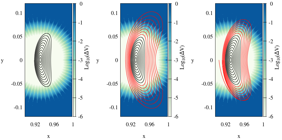
Figure 2: Lyapunov orbits of different amplitudes computed by normalizing the Hamiltonian in the Cartesian variables with the method (a) (left panel), method (b) (center panel) and method (c) (right panel). The initial conditions have been obtained from the normalized Cartesian Hamiltonian, while the orbits have been numerically computed by integrating the regularized Hamiltonian ${\cal K}_{E}$ in Eq. (10). On the background we plot with a color scale the logarithm of $\left|\Delta V_{N}\right|$ defined in (35). The orbits in black are those for which the energy error is in agreement with the normal form (see eq. (36) and Fig. 3).

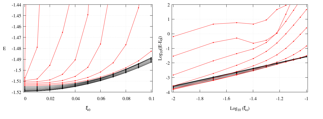
Figure 3: The curves in both panels represent the quantity $E$ defined in eq. (36) computed for $q_{0},p_{0}$ corresponding to a selected point in each Lyapunov orbit of Fig. 2, while $\eta=0$ and $\xi\in[0,0.1]$. The black and red curves correspond to the Lyapunov orbits represented in black and red respectively. We appreciate that only for the black curves the behaviour of $E$ is in agreement with eq. (36).

Aiming to investigate the limits of the normalizations implemented with the Cartesian variables, we represent the family of Lyapunov orbits $LL_{1}(E)$ at different values of the energy, computed from the normalization of the Hamiltonian expressed with these variables with the three different normalizing strategies (a), (b), (c), see Fig. 2. The starting point of any Hamiltonian normalization in Cartesian variables includes the computation of the Taylor expansion $V_{N}$ at order $N$ of the singular potential energy

$$V=-{\mu\over\sqrt{(x-1+\mu)^{2}+y^{2}}}$$

appearing in Hamiltonian (3). As already remarked, for $\mu=\mu_{J}$, the function $V$ has complex singularities located at $x=x_{L_{1}},y=\pm i\sigma\sim 0.06\pm i0.066...$. For the values of the energy $E$ that we consider, we need to perform normalizations for $N\in[20,30]$. In this range of $N$ the complex singularity affects the Taylor expansions for $y>0.066$. For example, by denoting with

$$\Delta V_{N}(x,y)=\left|V_{N}(x,y)-V(x,y)\right|,$$ (35)

an easy computation shows

$N$	$\Delta V_{N}\text{\small$(x_{L_{1}},0.066$)}$	$\Delta V_{N}\text{\small$(x_{L_{1}},0.08$)}$	$\Delta V_{N}\text{\small$(x_{L_{1}},0.1$)}$
20	$10^{-3}$	$5.5\ 10^{-2}$	$5.7$
30	$7.4\ 10^{-4}$	$0.28$	$270$

In order to check how this singularity affects the validity of the normal form expansions, in Fig. 2 we show the Lyapunov orbits corresponding to $E\in[-1.5193,-1.502]$ obtained from the normalization of the Cartesian Hamiltonian with the three strategies (a), (b), (c) for $N=30$. The orbits in Fig. 2 are obtained by numerically integrating an initial condition of the approximate Lyapunov orbit obtained from Eq. (6), without applying differential corrections. Due to the abundance of bibliography explaining this type of computations (see [4], [31] and references therein), we limit ourselves to present only the results. In the background we plot in color scale the value of the function $\log_{10}\left|\Delta V_{N}\right|$. With evidence, the largest reliable Lyapunov orbit obtained with the Cartesian variables strategy (a) (Fig. 2, left panel) is within the domain of the plane $x,y$ where the error function $\left|\Delta V_{N}(x,y)\right|$ is small. Instead, we observe that for the largest Lyapunov orbit obtained with the Cartesian variables-strategy (b) (Fig. 2, center panel), the amplitude is well beyond the limit of the complex singularity of $V$. As a matter of fact, the effect of the error due to the difference $\left|\Delta V_{N}\right|$ appears when we consider values of the hyperbolic variables $\xi,\eta\neq 0$. From the specific expression of the normal form $(b)$ (Eq. (22)), for any given $(q_{0},p_{0})$ we have:

$$E=E_{0}(q_{0},p_{0})+\xi^{2}A(q_{0},p_{0})+.....$$ (36)

and therefore we expect a quadratic growth of $E-E_{0}(q_{0},p_{0})$ with $\xi$. This behavior is confirmed only for the Lyapunov orbits in black in Fig. 2, center panel. Precisely, by choosing a sample point for each Lyapunov orbit of Fig. 2, given by $q_{0},p_{0},\xi=0,\eta=0$ in the normalized variables, in Fig. 3 we show the values of the energy $E$ computed for $\eta=0$ and $\xi\in[0,1/10]$. Only for the Lyapunov orbits represented in black we have an agreement between the curves of Fig. 3 and the law (36). The same behaviour is found for the normalization method (c) (Fig. 2, right panel). We conclude that the limit of the normalizations implemented with the Cartesian variables is given by $\left|1-\mu-x_{L_{1}}\right|$.

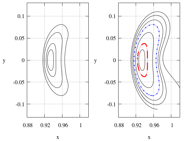
Figure 4: Lyapunov orbits of different amplitudes computed by normalizing the Levi-Civita Hamiltonian with the method (a) (left panel) and method (c) (right panel). The initial conditions have been obtained from the normalized Levi-Civita Hamiltonian, while the orbits have been numerically computed by integrating the non-normalized Hamiltonian ${\cal K}_{E}$.

Table 1: Norm of the remainder $R^{N}$ evaluated on the Lyapunov orbit for $E_{a}=-1.516$ (left columns) and for $E_{b}=-1.509$ (right columns), according to Eq. (32), produced with expansions limited to order ${\cal N}_{p}=27$ and normalization order $N=3,...,24$.

Red orbit Fig. 4		Blue orbit Fig. 4
$N$	$R^{N}$	X $N$	$R^{N}$
$3$	$1.61835\,{\scriptstyle\times 10}^{[}-5]$	X $3$	$7.28121\,{\scriptstyle\times 10}^{[}-4]$
$4$	$2.35741\,{\scriptstyle\times 10}^{[}-6]$	X $4$	$3.53145\,{\scriptstyle\times 10}^{[}-4]$
$5$	$4.90253\,{\scriptstyle\times 10}^{[}-7]$	X $5$	$2.61175\,{\scriptstyle\times 10}^{[}-4]$
$6$	$1.00808\,{\scriptstyle\times 10}^{[}-7]$	X $6$	$1.98361\,{\scriptstyle\times 10}^{[}-4]$
$7$	$2.34993\,{\scriptstyle\times 10}^{[}-8]$	X $7$	$1.45230\,{\scriptstyle\times 10}^{[}-4]$
$8$	$4.72191\,{\scriptstyle\times 10}^{[}-9]$	X $8$	$1.04454\,{\scriptstyle\times 10}^{[}-4]$
$9$	$2.13184\,{\scriptstyle\times 10}^{[}-9]$	X $9$	$8.94943\,{\scriptstyle\times 10}^{[}-5]$
$10$	$4.13041\,{\scriptstyle\times 10}^{[}-10]$	X $10$	$6.06359\,{\scriptstyle\times 10}^{[}-5]$
$11$	$1.51257\,{\scriptstyle\times 10}^{[}-10]$	X $11$	$4.88443\,{\scriptstyle\times 10}^{[}-5]$
$12$	$3.59044\,{\scriptstyle\times 10}^{[}-11]$	X $12$	$3.31315\,{\scriptstyle\times 10}^{[}-5]$
$13$	$8.67395\,{\scriptstyle\times 10}^{[}-12]$	X $13$	$2.28439\,{\scriptstyle\times 10}^{[}-5]$
$14$	$1.81004\,{\scriptstyle\times 10}^{[}-12]$	X $14$	$1.53451\,{\scriptstyle\times 10}^{[}-5]$
$15$	$5.38462\,{\scriptstyle\times 10}^{[}-13]$	X $15$	$1.14096\,{\scriptstyle\times 10}^{[}-5]$
$16$	$9.09849\,{\scriptstyle\times 10}^{[}-14]$	X $16$	$7.54539\,{\scriptstyle\times 10}^{[}-6]$
$17$	$2.32918\,{\scriptstyle\times 10}^{[}-14]$	X $17$	$5.71248\,{\scriptstyle\times 10}^{[}-6]$
$18$	$5.61067\,{\scriptstyle\times 10}^{[}-15]$	X $18$	$4.31952\,{\scriptstyle\times 10}^{[}-6]$
$19$	$2.70410\,{\scriptstyle\times 10}^{[}-15]$	X $19$	$3.64058\,{\scriptstyle\times 10}^{[}-6]$
$20$	$3.35487\,{\scriptstyle\times 10}^{[}-16]$	X $20$	$2.42248\,{\scriptstyle\times 10}^{[}-6]$
$21$	$1.67395\,{\scriptstyle\times 10}^{[}-16]$	X $21$	$2.22411\,{\scriptstyle\times 10}^{[}-6]$
$22$	$4.91488\,{\scriptstyle\times 10}^{[}-17]$	X $22$	$1.63076\,{\scriptstyle\times 10}^{[}-6]$
$23$	$1.75187\,{\scriptstyle\times 10}^{[}-17]$	X $23$	$1.31428\,{\scriptstyle\times 10}^{[}-6]$
$24$	$5.80105\,{\scriptstyle\times 10}^{[}-18]$	X $24$	$9.80338\,{\scriptstyle\times 10}^{[}-7]$

We therefore proceed to check that the normalization of the Hamiltonian expressed with the Levi-Civita variables overcomes this limit. First, in Fig. 4 we show the Lyapunov orbits computed using method (a) in the left panel and method (c) in the right panel. The initial conditions used for each case have been obtained from the normalized Levi-Civita Hamiltonian ${\cal K}^{(N)}_{E}$ in Eq. (19) at the specific energy value, and they were numerically integrated with the non-normalized Hamiltonian ${\cal K}_{E}$ (10). Thanks to the implementation of the normalization method in the regularized Levi-Civita Hamiltonian, with both methods we compute Lyapunov orbits of libration amplitudes larger than the threshold value $0.066...$ of the Cartesian normalizations. Then, the threshold value of the largest Lyapunov orbit depends also on the normalization method. In fact, with the method (c) we reach a larger value for the amplitude with respect to the method (a). The limiting factor for strategy (a) is clearly the large number of terms to eliminate to render the Hamiltonian in normal form. Since for the computation of the stable and unstable manifolds we are forced to use method (a), we have an indication of the improvement introduced by the Levi-Civita variables, which allow us to reach a libration amplitude of about $1.4\ \left|1-\mu-x_{L_{1}}\right|$.

With the sake of explaining the differences between these techniques, we provide a few specific examples of the normal forms computations. We consider here the computation of Lyapunov orbits for two specific values of the energy, the first corresponding to a small amplitude Lyapunov orbit ($E=E_{a}:=-1.516$) and the second corresponding to a moderate amplitude Lyapunov orbit ($E=E_{b}:=-1.509$). For reference, $LL_{1}(E_{a})$ is represented with a dashed red curve in Fig. 4, while $LL_{1}(E_{b})$ corresponds to the dotted blue orbit. We expect that small libration orbits imply small errors in the computation. This is confirmed by the computation of the norm of the remainders $R^{N}$ (evaluated according to Eq. (32)) of such orbits, represented in Table 1, for $N\in\{3,\ldots,24\}$, for the normalizing strategy (c).

Additionally, in Tables 2 and 3, we compare the normal forms obtained with the three strategies for the first two steps of the normalization, giving ${K_{3}}$ and ${K_{4}}$ respectively, for $LL_{1}(E_{b})$. Each entry of the tables refers to a specific monomial appearing in the normal form, for which it is given the integers $k_{1}$, $l_{1}$, $k_{2}$, $l_{2}$, indicated in which normal form it is present (out of the three strategies), and the associated coefficient $\alpha$.

Table 2: Normal form decomposition of ${K_{3}}$ for the example $LL_{1}(E_{a})$

monomial				strategy
$k_{1}$	$l_{1}$	$k_{2}$	$l_{2}$	(a)	(b)	(c)	$\alpha^{(3)}_{k_{1},l_{1},k_{2},l_{2}}$
0	0	0	3	x	x	x	$-0.239846$
0	1	0	2	x	x	x	$0.1371133+0.0334760\,\mathrm{i}\,$
0	3	0	0	x	x	x	$0.144918$
1	0	0	2	x	x	x	$0.0334760+0.1371133\,\mathrm{i}\,$
1	2	0	0	x	x	x	$-0.164176\,\mathrm{i}$
2	1	0	0	x	x	x	$0.164176$
3	0	0	0	x	x	x	$-0.144918\,\mathrm{i}$
0	0	1	2	x	x	x	$0.642141$
0	1	1	1	x	x	x	$-0.284350$
1	0	1	1	x	x	x	$-0.284350\,\mathrm{i}$
0	0	2	1	x	x	x	$-0.642141$
0	1	2	0	x	x	x	$0.1371133-0.0334760\,\mathrm{i}\,$
1	0	2	0	x	x	x	$-0.0334760+0.1371133\,\mathrm{i}\,$
0	0	3	0	x	x	x	$0.239846$
Total of terms				6	10	14

Table 3: Normal form decomposition of ${K_{4}}$ for the example $LL_{1}(E_{a})$

monomial				strategy
$k_{1}$	$l_{1}$	$k_{2}$	$l_{2}$	(a)	(b)	(c)	$\alpha^{(4)}_{k_{1},l_{1},k_{2},l_{2}}$
0	0	0	4	x	x	x	$-0.478035$	†
0	1	0	3	x	x	x	$0.732257+1.135126\,\mathrm{i}$	†
0	2	0	2	x	x	x	$-0.342835-1.071743\,\mathrm{i}$	†
0	4	0	0	x	x	x	$0.0583902$	†
1	0	0	3	x	x	x	$1.135126+0.732257\,\mathrm{i}$	†
1	1	0	2	x	x	x	$-2.41906\,\mathrm{i}$	†
1	3	0	0	x	x	x	$-1.81534\,\mathrm{i}$	†
2	0	0	2	x	x	x	$0.342835-1.071743\,\mathrm{i}$	†
2	2	0	0	x	x	x	$-3.37708$	†
3	1	0	0	x	x	x	$1.81534\,\mathrm{i}$	†
4	0	0	0	x	x	x	$0.0583902$	†
0	0	1	3	x	x	x	$2.23041$	†
0	1	1	2	x	x	x	$-2.86948-1.59924\,\mathrm{i}$	†
0	2	1	1	x	x	x	$2.31725$	⋆
1	0	1	2	x	x	x	$-1.59924-2.86948\,\mathrm{i}$	†
1	1	1	1	x	x	x	$2.55115\,\mathrm{i}$	⋆
2	0	1	1	x	x	x	$-2.31725$	⋆
0	0	2	2	x	x	x	$3.75798$	∙
0	1	2	1	x	x	x	$-2.86948-1.59924\,\mathrm{i}$	†
0	2	2	0	x	x	x	$-0.342835+1.071743\,\mathrm{i}$	†
1	0	2	1	x	x	x	$-1.59924+2.86948\,\mathrm{i}$	†
1	1	2	0	x	x	x	small $-2.41906\,\mathrm{i}$	†
2	0	2	0	x	x	x	$0.342835+1.071743\,\mathrm{i}$	†
0	0	3	1	x	x	x	$2.23041$	†
0	1	3	0	x	x	x	$-0.732257+1.135126\,\mathrm{i}$	†
1	0	3	0	x	x	x	$1.135126-0.732257\,\mathrm{i}$	†
0	0	4	0	x	x	x	$-0.478035$	†
Total of terms				9	23	27

From Table 2, we can see that the less demanding normalization schemes (b) and (c) provide normal forms with many more terms than the strategy (a). At this step of normalization, there are no differences in the coefficients, since the three strategies are applied to the same initial expansion (the terms $K_{0}$ and $K_{2}$ are common to the three). When performing the following step, since now the schemes are applied also on $K_{3}$, the values of the coefficients start differing from strategy to strategy. The coefficients in Table 2 refer to the normalization by strategy (c), and we denote with different symbols the monomials whose coefficient has a different value for the strategy (a) ($\bullet$), the strategy (b) ($\dagger$) or both ($\star$). As we proceed with the normalizations, the resulting $K_{j}$ are different from each other. We also notice the increase in the amount of terms from step $3$ to $4$. This effect is evident also in Table 4, which summarizes the information related to the normal form computation (following strategy (c)) for the set of Lyapunov orbits appearing in Fig. 4 (right panel). The information provided corresponds to: the values of $E$, the order of the initial polynomial expansion $N_{p}$, the normalization order $N$, the amount of terms of the normal form ${\cal K}_{E}^{(N)}$ and of the remainder ${\cal R}_{E}^{(N)}$ at order $N$, and the maximum distance that the orbit reaches with respect to the position of $L_{1}$.

Table 4: Normalization information for the orbits presented in Fig. 4.

$E$	$N_{p}$	$N$	term ${\cal K}^{(N)}_{E}$	terms ${\cal R}^{(N)}_{E}$	Max ampl
$-1.518$	13	10	$1658$	$2056$	$2.38{\scriptstyle\times 10}^{[}-2]$
$-1.516$	13	10	$1658$	$2056$	$3.83{\scriptstyle\times 10}^{[}-2]$
$-1.512$	19	16	$6967$	$5335$	$6.53{\scriptstyle\times 10}^{[}-2]$
$-1.509$	21	18	$10200$	$6924$	$8.54{\scriptstyle\times 10}^{[}-2]$
$-1.507$	25	22	$19869$	$10990$	$9.73{\scriptstyle\times 10}^{[}-2]$
$-1.505$	33	30	$57843$	$23346$	$1.08{\scriptstyle\times 10}^{[}-1]$
$-1.504$	33	30	$57843$	$23346$	$1.17{\scriptstyle\times 10}^{[}-1]$

As for increasing energies the periodic orbits have larger amplitudes, it is necessary to use larger normalizations orders (see Table 1). Notice, for instance, that a variation of $\sim 1$% in the energy (from $E=-1.518$ to $E=-1.505$) requires to use a normalization order 3 times larger, and the associated normal form is 35 times longer. This exponential growth makes hardly tractable the computation of these normal forms for larger values of the energy.

4 Numerical computation of the stable tubes manifolds

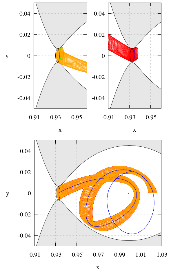
Figure 5: Representation of the inner and outer stable tubes for $E=-1.5193$. Top panels: the Lyapunov orbit $LL_{1}(E=-1.5193)$ (black curve), initial conditions of the outer tube (green curve) and the inner tube (blue curve), orbits of the outer tube (orange) and the inner tube (red) integrated forward in time. Bottom panel: Outer (orange) and inner (red) tubes integrated backward in time, almost overlapped (see text for discussion), and the invariant stable manifold emanating from $LL_{1}$ (blue curve, appearing also in the top left panel of Fig. 1). The shaded area represents the realm of forbidden motions for this value of the energy.

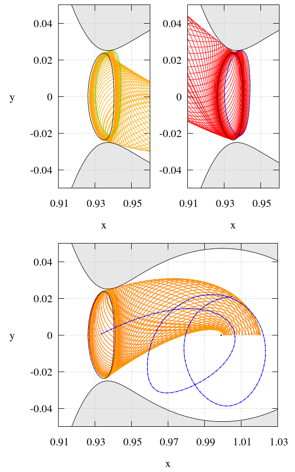
Figure 6: As Fig. 5, for $E=-1.5183$.

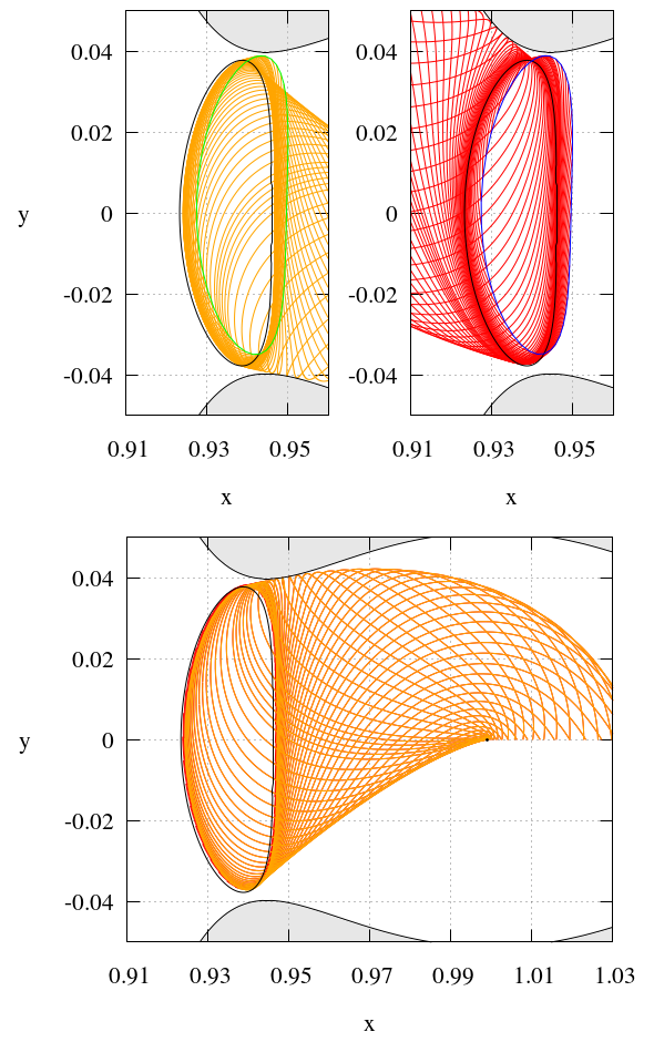
Figure 7: As Fig. 5, for $E=-1.5167$.

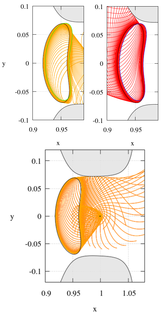
Figure 8: As Fig. 5, for $E=-1.5113$.

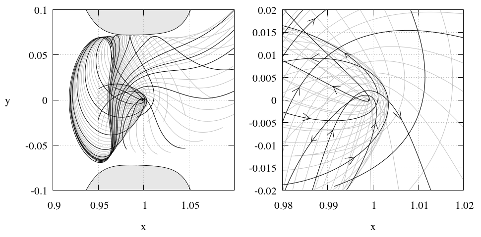
Figure 9: Left panel: Same as Fig. 8 where some orbits are highlighted in bold black curves. Right panel: Zoomed-in of the left panel, in the vicinity of the primary $P_{2}$. The arrows indicate the sense of motion backward in time. Some of the orbits circulate clockwise, while others do it counter-clockwise.

In Fig. 5, 6, 7 and 8, we represent the inner and outer stable tubes computed using the normalized Levi-Civita Hamiltonian as explained in Section 2 (see Eq. (34) and related discussion), for $E=-1.5193$, $-1.5183$, $-1.5167$, $-1.5113$ respectively. For each value of $E$, the inner/outer tubes are obtained first by considering $\xi_{0}=\pm 10^{-4}<<\eta_{0}=10^{-2}$, and by numerically computing a set of points $(q_{j},p_{j})$ ($j=0,\ldots,30$) sampling the level set

$${\cal K}^{(N)}_{E}(\xi_{0},q,\eta_{0},p)=0.$$

Then, we compute the image of all the points $(\xi_{0},q_{j},\eta_{0},p_{j})$ in the Levi-Civita variables $u,U$. Finally, the tubes are obtained by numerically integrating the Hamilton’s equation of the Levi-CivitaHamiltonian ${\cal K}_{E}(u,U)$ for these initial conditions.

On the top panels of each figure we represent separately the orbits with initial conditions in the inner tube (blue line) and the orbits with initial conditions in the outer tube (green line). When the initial conditions on the outer stable tube are integrated forward in time, as it happens in the top panels, initially they approach the Lyapunov orbit (black curve), but then the orbits of the outer stable tube (orange orbits) bounce back, while the orbits of the inner stable tube (red orbits) transit to the left of the Lyapunov orbit. This mechanism allows us to identify one tube from the other. When integrated backward in time (bottom panels of Fig. 5, 6, 7, 8), the orbits of both inner and outer stable tubes almost overlap, indicating the location of the invariant stable manifold.

Figures 5 and 6 show the traditional behavior for the stable manifold, as described at (ii) in Section 1. When integrated backward in time, both tubes fold around Jupiter clockwise, following the sense of the collapsed invariant manifold emanating from $LL_{1}(E_{1})$ (blue line in the bottom panels), $W^{s}_{1}(E_{1})$. The smaller the value of the energy is, the better $W^{s}_{1}(E_{1})$ represent the behavior of the tube manifold, as it is evident from comparing the two figures. The limit of this representation takes place when the stable tube manifold allows for collisions with the planet. In Fig. 7 we present a stable manifold that, while still folding clockwise, passes very close to $P_{2}$. It is natural to expect that, by increasing the energy, the stable manifold is such that some orbits eventually collide with $P_{2}$. This is clearly visualized in Fig. 8 and, particularly, in 9. For the energy $E=-1.5113$, we show that the manifold embraces the position of the planet, therefore allowing possible collisions with it. In the right panel of Fig. 9 we show some of the orbits belonging to the manifold, indicating with arrows the sense of the orbit when integrated backward in time. We see that, besides passing extremely close to the singularity, the orbits can either revolve around the $P_{2}$ either clockwise or counter-clockwise, indicating that this value of the energy is, already, a good representation of orbits of type (iii) (see description in Introduction).

5 Conclusions

In this work, we studied the transition from non collisional to possibly collisional orbits as a outcome of the change in the structure of the tubes manifolds emanating from the Lyapunov orbits of the CR3BP for the Sun-Jupiter system. To this aim, we constructed a normal form of the Levi-Civita Hamiltonian, at a partially hyperbolic fictitious equilibrium. The normalization of the Levi-Civita Hamiltonian, which is regular at the position of the planet, allows us to reach values of the energy not investigated before via the traditional normalizations of the CR3BP Hamiltonian in Cartesian variables. We found that, for suitably large values of the energy, the tubes manifolds emanating from the horizontal Lyapunov orbits may contain orbits that collide with the secondary body before performing a full circulation around it (when integrated backwards from the Lyapunov orbit), or can revolve either clockwise or counter-clockwise around $P_{2}$. We established that, for $\mu=\mu_{J}$, the transition takes place for values of the energy larger than $E>-1.5167$. We expect this threshold to be relevant for future studies of dynamics of temporary trapped comets and/or for space mission design.

As future work, we plan to extend the present work to the spatial restricted three–body problem. The Levi-Civita regularization is extended to the spatial case by the Kustaanheimo-Stiefel regularization,

$$X =u_{1}^{2}-u_{2}^{2}-u_{3}^{2}+u_{4}^{2}$$ (37)

$$Y =2(u_{2}u_{2}-u_{3}u_{4})$$

$$Z =2(u_{1}u_{3}+u_{2}u_{4})$$

$$dt =\left|u\right|^{2}d\tau$$

see [39], [40]. Let us denote by ${\cal K}_{E}(u,U)$ the Hamiltonian representing the Kustaanheimo-Stiefel regularization (see for example [34], [41] for a detailed derivation). For values $E>E_{L_{1}}$, the fictitious equilibrium found in the regularized planar problem, $u_{*}=(0,u_{2_{*}}^{\phantom{3}}\!)$, $U_{*}=(-2u_{2_{*}}^{\phantom{3}}\!{}^{3},0)$, extends to an equilibrium of Hamilton equations of the Kustaanheimo-Stiefel Hamiltonian, $u_{*}=(0,u_{2_{*}}^{\phantom{3}}\!,0,0)$, $U_{*}=(-2u_{2_{*}}^{\phantom{3}}\!,0,0,0)$, satisfying the bi-linear equation $\ell(u_{*},U_{*})=0$ where $\ell(u,U)=u_{4}U_{1}-u_{3}U_{2}+u_{2}U_{3}-u_{1}U_{4}$. In principle, this be used to define a normalizing transformation as done in the present work. On the other hand, the internal symmetry of the Kustaanheimo-Stiefel transformation requires specific adaptations, which will be the subject of future work.

Appendix

A1) Computing the equilibria $(u_{*},U_{*})$. The equilibrium points of ${\cal K}_{E}$, satisfying $u_{1}=0$ (which is the condition granting $y=2u_{1}u_{2}=0$, $x=x_{2}+u_{1}^{2}-u_{2}^{2}<x_{2}$) and $u_{2}\in(-1,0)$ ($u_{2}=-1$, $u_{2}=0$ locate the equilibrium on the primary body $P_{1}$ and $P_{2}$ respectively) are the solutions of

$$\left.\frac{\partial{\cal K}_{E}}{\partial U_{1}}\right|_{u_{1}=0} =\frac{1}{4}\,(U_{1}+2u_{2}^{3})=0\leavevmode\nobreak\ \leavevmode\nobreak\ ,$$ (38)

$$\left.\frac{\partial{\cal K}_{E}}{\partial U_{2}}\right|_{u_{1}=0} =\frac{1}{4}\,U_{2}=0\leavevmode\nobreak\ \leavevmode\nobreak\ ,$$

$$\left.\frac{\partial{\cal K}_{E}}{\partial u_{1}}\right|_{u_{1}=0} =-\frac{1}{2}\,U_{2}\,u_{2}^{2}=0\leavevmode\nobreak\ \leavevmode\nobreak\ ,$$

$$\left.\frac{\partial{\cal K}_{E}}{\partial u_{2}}\right|_{u_{1}=0} =u_{2}\bigg{[}-2\big{(}E+\frac{1}{2}(1-\mu)^{2}\big{)}-3u_{2}^{4}\Big{.}$$

$$+\frac{3}{2}u_{2}^{2}\,(U_{1}+2u_{2}^{3})$$

$$-(1-\mu)\,u_{2}\,\big{(}-2u_{2}-\frac{-2u_{2}+2u_{2}^{3}}{(1-2u_{2}^{2}+u_{2}^{4})^{3\over 2}}\big{)}$$

$$\Big{.}-2(1-\mu)\big{(}-u_{2}^{2}+\frac{1}{\sqrt{1-2u_{2}^{2}+u_{2}^{4}}}\big{)}\bigg{]}=0\leavevmode\nobreak\ \leavevmode\nobreak\ .$$

We first notice that the first equation of this system provides $U_{1}=-2u_{2}^{3}$, while the second and the third ones are solved if $U_{2}=0$. Then, by using $U_{1}=-2u_{2}^{3}$ and noticing that since $u_{2}^{2}\in(0,1)$ we have $\sqrt{1-2u_{2}^{2}+u_{2}^{4}}=1-u_{2}^{2}$, the last equation is solved by $u_{2}$ satisfying $F(u_{2},E)=0$, where the function $F$ is defined in (13). A2) Solutions of the equation $F(u_{2},E)=0$. To solve equation $F(u_{2},E)=0$ we first re-write it in the form

$$E= f(u_{2},\mu)$$

$$:= \text{\small$-{3\over 2}u_{2}^{4}+(1-\mu)\left(2u_{2}^{2}-{u_{2}^{2}\over(1-u_{2}^{2})^{2}}-{1\over 1-u_{2}^{2}}\right)-{(1-\mu)^{2}\over 2}$},$$

¿From standard calculus, we have

$${\partial f\over\partial u_{2}}=-6u_{2}^{3}-4(1-\mu)u_{2}^{3}{3-3u_{2}^{2}+u_{2}^{4}\over(1-u_{2}^{2})^{3}}>0$$

for all $\mu\in[0,1/2]$ and $u_{2}\in(-1,0)$. As a consequence there is a strictly monotone increasing function $E:=E(u_{2})$ defined for $u_{2}\in(-1,0)$ such that $F(u_{2},E(u_{2}))=0$. Since we know that the Lyapunov orbits exist only for $E\geq E_{1}$, we restrict the domain of $E(u_{2})$ to the interval $[-\sqrt{x-x_{L_{1}}},0)$ and we define the inverse $a(u_{2})$ of $E(u_{2})$:

$$\Big{[}E_{1},E_{*}\Big{)}\longrightarrow[-\sqrt{x-x_{L_{1}}},0)$$

$$u_{2}\longmapsto(u_{2_{*}}^{\phantom{3}}\!)$$

where $E_{*}$ has been defined in (14). A3) Linearization of the Hamilton equations of ${\cal K}_{E}$ at $u_{*},U_{*}$. The Jacobian matrix of the Hamilton vector field of ${\cal K}_{E}$ at $(u_{*},U_{*})$ is

$$M=\begin{pmatrix}0&\frac{3(u_{2_{*}}^{\phantom{3}}\!)^{2}}{2}&\frac{1}{4}&0\\ -\frac{(u_{2_{*}}^{\phantom{3}}\!)^{2}}{2}&0&0&\frac{1}{4}\\ \Gamma&0&0&\frac{(u_{2_{*}}^{\phantom{3}}\!)^{2}}{2}\\ 0&-2\Gamma+(u_{2_{*}}^{\phantom{3}}\!)^{4}&-\frac{3(u_{2_{*}}^{\phantom{3}}\!)^{2}}{2}&0\end{pmatrix}\leavevmode\nobreak\ ,$$ (39)

with

$$\Gamma=-(u_{2_{*}}^{\phantom{3}}\!)^{4}+4(u_{2_{*}}^{\phantom{3}}\!)^{2}(1-\mu)\left(1-\frac{1}{(1-(u_{2_{*}}^{\phantom{3}}\!)^{2})^{3}}\right).$$

As a consequence, the matrix $M$ has four eigenvalues:

$$\gamma =\pm{1\over\sqrt{8}}\sqrt{-\Gamma-5(u_{2_{*}}^{\phantom{3}}\!)^{4}\pm\sqrt{9\Gamma^{2}-22(u_{2_{*}}^{\phantom{3}}\!)^{4}\Gamma-15(u_{2_{*}}^{\phantom{3}}\!)^{8}}}$$ (40)

$$:=\pm\sqrt{{A\pm\sqrt{B}}\over 8}\leavevmode\nobreak\ .$$

whose nature is determined by the values of the functions $A,B$. From standard calculus, for all $\mu\in(0,1/2)$ and $u_{2}\in(u_{2_{*}}^{\phantom{3}}\!,0)$ one proves: $\Gamma<0$, $B>0$, $B>\Gamma+5(u_{2_{*}}^{\phantom{3}}\!)^{4}$. As a consequence, the matrix $M$ has a couple of real eigenvalues $\pm\lambda$ and a couple of purely imaginary numbers $\pm i\omega$. Moreover, for $a$ going to zero, both $\lambda,\omega$ tend to zero as (a constant multiplying) $(u_{2_{*}}^{\phantom{3}}\!)^{2}$. A4) Diagonalization of the quadratic part of ${\cal K}_{E}$. Let ${v}_{i}$, $i=1,\ldots,4$, the four eigenvectors of $M$; matrix $A$ is constructed as :

$$A=(c_{1}{v}_{3}^{t},\,c_{2}{v}_{1}^{t},\,\mathrm{i}c_{1}{v}_{4}^{t},\,c_{2}{v}_{2}^{t})$$ (41)

where $c_{1},c_{2}\in\mathbb{C}$ are chosen to satisfy the symplectic condition $A^{t}{\mathbb{J}}A={\mathbb{J}}$, where ${\mathbb{J}}$ denotes the standard symplectic matrix.

References

• [1] C.ย Conley. Low energy transit orbits in the restricted three-body problem. SIAM J. Appl. Math., 16(4):732โ€“746, 1967.
• [2] R.ย Greenberg, A.ย Carusi, and G.B. Valsecchi. Outcomes of planetary close encounters: A systematic comparison of methodologies. Icarus, 75(1):1โ€“29, 1988.
• [3] P.W. Chodas. Orbit uncertainties, keyholes and collision probabilities. Bull. Astron. Soc., 31:1117, 1999.
• [4] A.ย Jorba and J.ย Masdemont. Dynamics in the center manifoldof the restricted three-body problem. Phys. D, 132:189โ€“213, 1999.
• [5] C.ย Simรณ. Dynamical systems methods for space missionson a vicinity of collinear libration points. In Simรณ, C., editor, Hamiltonian Systems with Three or More Degrees of Freedom, NATO Adv. Sci. Inst. Ser. C Math. Phys. Sci., volume 533, pages 223โ€“241, 1999.
• [6] G.B. Valsecchi. Planetary close encounters: the engine of cometary orbital evolution. In Steves B.A., Roy A.E. eds, The dynamics of small bodies in the Solar System, Kluwer Acad. Pub, pages 187โ€“196, 1999.
• [7] G.ย Gรณmez, A.ย Jorba, J.ย Masdemont, and Simรณ C. Dynamics and Mission Design NearLibrationPoint Orbits, Vol. 3: Advanced Methods for Collinear Points. World Scientific ed., Singapore, 2000.
• [8] G.B. Valsecchi, A.ย Milani, G.F. Gronchi, and S.R. Chesley. Resonant returns to close approaches: analytical theory. Astron. Astrophys., 408(3):1179โ€“1196, 2003.
• [9] J.J. Masdemont. High-order expansions of invariant manifolds of libration point orbtis with applications to mission design. Dyn. Sys., 20(1):59โ€“113, 2005.
• [10] G.B. Valsecchi. Close encounters and collisions of near-earth asteroids with the earth. C.R. Physique, 6(3):337โ€“344, 2005.
• [11] W.S. Koon, M.W. Lo, J.E. Marsden, and S.D. Ross. Dynamical Systems, The Three-Body Problem and Space Mission Design. Springer Verlag, New York, 2007.
• [12] E.ย Lega, M.ย Guzzo, and C.ย Froeschlรฉ. Detection of close encounters and resonances in three-body problems through levi-civita regularization. MNRAS, 418:107โ€“113, 2011.
• [13] G.ย Gomez, W.S. Koon, M.W. Lo, J.E. Marsden, J.ย Masdemont, and S.D. Ross. Connecting orbits and invariant manifolds in the spatial restricted three-body problem. Nonlinearity, 17:1571โ€“1606, 2004.
• [14] A.ย Zanzottera, G.ย Mingotti, R.ย Castelli, and M.ย Dellnitz. Intersecting invariant manifolds in spatial restricted three-body problems: design and optimization of earth-to-halo transfers in the sun-earth-moon scenario. Commun. Nonlin. Science Num. Sim., 17(2):832โ€“843, 2012.
• [15] M.ย Guzzo and E.ย Lega. On the identification of multiple close-encounters in the planar circular restricted three body problem. MNRAS, 428:2688โ€“2694, 2013.
• [16] Gronchi G. and G.ย Valsecchi. On the possible values of the orbit distance between a near-earth asteroid and the earth. MNRAS, 429(3):2687โ€“2699, 2013.
• [17] M.ย Guzzo and E.ย Lega. Evolution of the tangent vectors and localization of the stable andunstable manifolds of hyperbolic orbits by fast laypunov indicator. SIAM J. Appl. Math., 74(4):1058โ€“1086, 2014.
• [18] A.ย Celletti, G.ย Pucacco, and D.ย Stella. Lissajous and halo orbits in the restricted three-body problem. J. Nonlinear Science, 25(2):343โ€“370, 2015.
• [19] M.ย Guzzo and E.ย Lega. A study of the past dynamics of comet 67p/churyumov-gerasimenko with fast lyapunov indicators. Astron. Astrophys., 579(A79):1โ€“7, 2015.
• [20] M.ย Guzzo and E.ย Lega. Scenarios for the dynamics of comet 67p/churyumov-gerasimenko over the past 500 kyr. MNRAS, 469:S321โ€“S328, 2017.
• [21] E.ย Lega and M.ย Guzzo. Three-dimensional representations of the tube manifolds of the planar restricted three-body problem. Phys. D, 352:41โ€“53, 2016.
• [22] M.ย Guzzo and E.ย Lega. Geometric chaos indicators and computations of the spherical hypertube manifolds of the spatial circular restricted three-body problem. Phys. D, 373:35โ€“58, 2018.
• [23] E.J. ร–pik. Interplanetary Close Encounters. Elsevier, New York, 1976.
• [24] G.B. Valsecchi. Close encounters in รถpikโ€™s theory. In Benest D., Froeschlรฉ C. eds, Singularities in Gravitational Systems, pages 145โ€“178, 2002.
• [25] G.ย Tommei. Canonical elements for รถpik theory. Cel. Mech. Dyn. Astron., 94:173โ€“195, 2006.
• [26] G.B. Valsecchi, Cl. Froeschlรฉ, and R.ย Gonczi. Modelling close encounters with รถpikโ€™s theory. Planet. Space Science, 45(12):1561โ€“1574, 1997.
• [27] R.ย Moeckel. Isolating blocks near the collinear relative equilibria of the three-bodyproblem. Trans. of the Am. Math. Soc., 356:4395โ€“4425, 2004.
• [28] R.L. Anderson, R.W. Easton, and M.W. Lo. Isolating blocks as computational tools in the circular restricted three-body problem. Phys. D, 343:38โ€“50, 2017.
• [29] A.ย Carusi and G.B. Valsecchi. Temporary satellite captures of comets by jupiter. Astron. Astrophys., 94:226โ€“228, 1981.
• [30] B.ย Krauskopf and H.M. Osinga. Computing geodesic level sets of global (un)stable manifolds of vector fields. SIAM J. Appl. Dyn. Syst, 2(4):546โ€“569, 2003.
• [31] A.ย Giorgilli. On a theorem of lyapounov. Rendiconti dellโ€™Instituto Lombardo Academia di Scienze e Lettere, 146:133โ€“160, 2012.
• [32] T.ย Levi-Civita. Sur la rรฉgularisation qualitative du problรฉme restreint des trois corps. Acta Math., 30:305โ€“327, 1906.
• [33] C.ย Simรณ and T.J. Stuchi. Central stable/unstable manifolds and the destruction of kam tori in the planar hill problem. Phys. D, 140:1โ€“32, 2000.
• [34] F.ย Cardin and M.ย Guzzo. Integrability of the spatial three-body problem near collisions (an announcement). Rend. Lincei, Mat. Appl., 30:195โ€“204, 2019.
• [35] K.R. Meyer, G.R. Hall, and D.ย Offin. Introduction to Hamiltonian Dynamical Systems and the N-Body Problem. Springer-Verlag, 2009.
• [36] J.A. Sanders, F.ย Verhulst, and Murdock J. Averaging Methods in NonLinear Dynamical Systems. Springer-Verlag, 2007.
• [37] C.ย Efthymiopoulos. Canonical perturbation theory, stability and diffusion in hamiltonian systems: applications in dynamical astronomy. In Proc. Third La Plata School on Astronomy and Geophysics, pages 3โ€“147, 2011.
• [38] A.ย Giorgilli. Notes on exponential stability of hamiltonian systems. In Dynamical Systems, part I, Pubb. Cent. Ric. Mat. Ennio Giorgi, Scuola Norm. Sup., Pisa, pages 87โ€“198, 2003.
• [39] P.ย Kustaanheimo. Spinor regularisation of the kepler motion. Annales Universitatis Turkuensis A 73, 1-7, 73:1โ€“7, 1964.
• [40] P.ย Kustaanheimo and E.L. Stiefel. Perturbation theory of kepler motion based on spinor regularization. J. fur die Reine und Angewandte Mathematik, 218:204โ€“219โ€“569, 1965.
• [41] F.ย Cardin and M.ย Guzzo. Integrability of the spatial three-body problem near collisions. Preprint arXiv:1809-01257, 2018.