From top-hat masking to smooth transitions: P-filter and its application to polarized microwave sky maps

Abstract

In CMB science, the simplest idea to remove a contaminated sky region is to multiply the sky map with a mask that is 0 for the contaminated region and 1 elsewhere, which is also called a top-hat masking. Although it is easy to use, such top-hat masking is known to suffer from various leakage problems. Therefore, we want to extend the top-hat masking to a series of semi-analytic functions called the P-filters. Most importantly, the P-filters can seamlessly realize the core idea of masking in CMB science, and, meanwhile, guarantee continuity up to the first derivative everywhere. The P-filters can significantly reduce many leakage problems without additional cost, including the leakages due to low-, high-, and band-pass filtering, and the E-to-E, B-to-B, B-to-E, and E-to-B leakages. The workings of the P-filter are illustrated by using the WMAP and Planck polarization sky maps. By comparison to the corresponding WMAP/Planck masks, we show that the P-filter performs much better than top-hat masking, and meanwhile, has the potential to supersede the principal idea of masking in CMB science. Compared to mask apodization, the P-filter is “outward”, that tends to make proper use of the region that was marked as 0; whereas apodization is “inward”, that always kills more signal in the region marked as 1.

1 Introduction

During the last several years, analysis of the Cosmic Microwave Background (CMB) polarization became one of the primary occupations for the Planck [1, 2, 3] and forthcoming space/ground based experiments [4, 5, 6, 7]. The polarized CMB signal is usually characterized in terms of the Stokes parameters Q and U and contains unique information about the properties of the early Universe, especially cosmological gravitational waves (CGW).

Standard CMB analysis techniques involve transformation of the Q and U Stokes parameters into scalar (E) and pseudo-scalar (B) modes [8, 9], where the B-mode is due only to CGW, lensing effects, and residuals from foregrounds. The contribution of the CGW into the CMB B-mode is characterized by the parameter $r$, the ratio of tensor-to-scalar modes, where the term “tensor” corresponds to the power spectrum of the cosmological gravitational waves, and “scalar” describes the power spectrum of primordial adiabatic perturbations, which are responsible for the formation the galaxies and Large Scale Structure of matter in an expanding Universe. The most stringent constraint, given by the BICEP2-KECK/Planck joint data analysis, is $r<0.07$ [10]. Bearing in mind the target of constraining $r$ to $10^{-4}$$\sim$$10^{-3}$, we should not only significantly increase the sensitivity of experiments but also understand the properties of the polarized foregrounds and systematics at least by 3-4 orders of magnitude better than now. At the same time we need to revise some aspects of data processing, like masking, band passing, apodization etc., which could be the potential sources of uncertainty for extraction of the B-mode of polarization at the level of $r\sim 10^{-4}$. In this work, we focus on improving the masking technique.

In CMB science, the basic and most important idea to determine the shape of a mask can be described by just one sentence: the mask should cover the brightest pixels because they are contaminated by the foreground. This idea was explicitly adopted by the WMAP team in [11], where they use temperature thresholds to define the mask regions; it was also adopted by the Planck team, as we shall see in Section 2.2. Normally, further adjustment of the region definition is needed to, e.g., make the edge flatter, reduce the number of tiny holes, block missing pixels, cover the regions with strong systematics, etc.

Once the region is defined, masking is normally done by keeping the accepted region unchanged and zeroing the rest, which is called top-hat masking. The mask’s profile is evidently non-analytic at the boundary. For temperature anisotropy such non-analyticity is less critical in comparison with the case of polarization, where the discontinuity of the first derivative at the boundary plays an important role in mixing the E and B components. To minimize this effect, it was proposed by [12] to smooth the mask boundary and restore the analyticity of the mask. However, there are many smoothing schemes and an even larger number of parameters, leaving the optimal choice not at all obvious.

Another problem of top-hat masking is that it indiscriminately kills all pixels in the rejected region. However, those pixels certainly have different levels of foreground contamination, thus it is questionable to kill them all. This problem can not be solved by ordinary ways of smoothing the mask, because they are done after the mask was produced. However, it can be perfectly solved by the P-filter method introduced in this work.

In this paper, the P-filter is designed as a natural extension of top-hat masking that seamlessly implements the most important idea of masking in CMB science. The P-filter can be seen as a family of semi-analytic functions defined with two parameters: the threshold $P_{t}$, which implements the principal idea of masking; and the rank parameter $a$, which determines the shape of the filter. In the pixel domain, the P-filter essentially weights the pixels above and below a given threshold differently. The shape of the filter is automatically compatible with the actual map, suppressing the brightest pixels, while preserving continuity of the first derivative everywhere. It is also much easier to use the P-filter with maps having varying resolutions: changing the resolution of a top-hat mask is not necessarily straightforward, but a P-filter can be conveniently regenerated in a new resolution using identical parameters, with all preferable features preserved.

Throughout this paper, unless mentioned elsewhere, we will use the WMAP 9-year and Planck 2018 maps with $N_{side}=512$ smoothed to an angular scale of $1^{\circ}$. The outline of the paper is the following: in Section 2 we introduce the mathematical definition of the P-filter family and provide illustrating examples, and in Section 3, we explain how to construct a common P-filter for varies frequency bands. In Section 4 we explore a range of advantages P-filters have, and in Section 5 we show example of how to optimize the filter parameters based on a specific requirement. Finally, a brief discussion is given in Section 6.

2 Definition of the P-filter family and examples

2.1 Definition of the P-filter

The P-filter family proposed here consists of a set of filters defined as follows (bold letters stand for sky maps):

$$\mathbf{k}(P_{t}) = \left\{\begin{array}[]{lr}1&(\mathbf{P}\leq P_{t})\\ \left[1+\log\left(\frac{\mathbf{P}}{P_{t}}\right)\right]\frac{P_{t}}{\mathbf{P}}&(\mathbf{P}>P_{t})\end{array}\right.$$

$$\mathbf{k}(a,P_{t}) = \mathbf{k}(P_{t})^{a}$$ (2.3)

$$\mathbf{P}^{\prime} = \mathbf{k}(a,P_{t})\cdot\mathbf{P},$$

where $P_{t}$ is the threshold, $a$ is the filter rank, $\mathbf{P}$ is the input polarization intensity map, and $\mathbf{P^{\prime}}$ is the filtered map. $\mathbf{k}(P_{t})$ represents the simplest form of the filter kernel with rank $a=1$, and $\mathbf{k}(a,P_{t})$ covers all possible shapes of the filter kernels in terms of weight maps with the same resolution as $\mathbf{P}$.

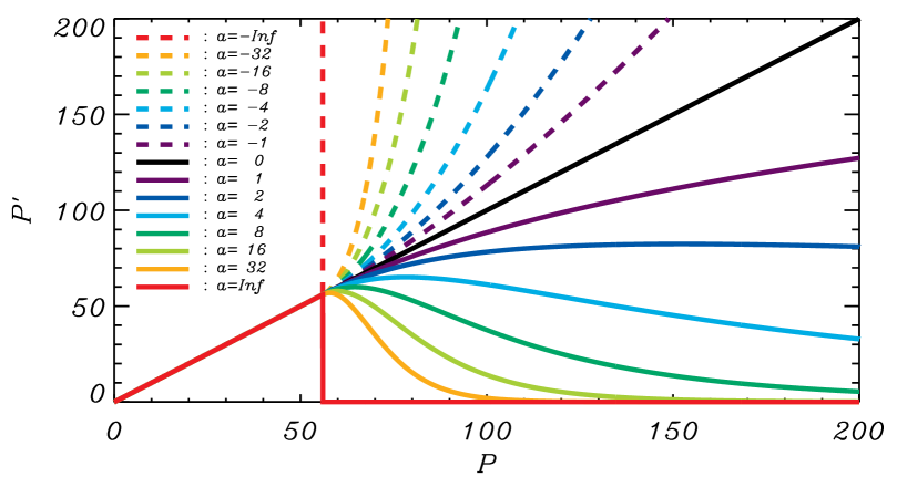
Figure 1: Profiles of P-filters from Eq. 2.1, with various ranks $a$ and the arbitrary choice of $P_{t}\equiv 56$ $\mu$K as example. The horizontal axis is the input polarization intensity, and the vertical axis is the filtered polarization intensity. $a=0$ corresponds to “no filtering”, and $a=\infty$ is top-hat masking.

According to the definition, the sky region with $\mathbf{P}<P_{t}$ will not change, while other regions will be suppressed by the factor $\mathbf{k}(a,P_{t})$. Note that the P-filters are defined directly on $\mathbf{P}$, where $\mathbf{P}$ can be any kind of data, even , e.g., time series data. This means the P-filters potentially have much wider application than merely in CMB science.

The first derivative of the filter function for $\mathbf{P}\geq P_{t}$ is:

$$\frac{dP^{\prime}}{dP}=\left(\frac{P_{t}}{P}\right)^{a}\left(1+\log\frac{P}{P_{t}}\right)^{a-1}\left[1+(1-a)\log\frac{P}{P_{t}}\right].$$ (2.4)

For any finite rank $a$, Eq. 2.4 is always equal to 1 at $P_{t}$, no matter calculated from the left or the right side. Thus the filter function is always continuous to the first derivative. However, discontinuity of the filter does occur for the second derivative, thus it is of differentiability class $C^{1}$ and we call it semi-analytic. Continuity of the whole family up to the first derivative everywhere is a desirable feature, e.g., with special design, it helps to prevent the EB-leakage [12].

In Figure 1, we illustrate the shapes of the P-filter functions when the rank $a$ varies from $-\infty$ to $+\infty$. From this figure, it is easy to see how the P-filter family covers the entire region where $\mathbf{P}>P_{t}$. Each point $(P,P^{\prime})$ in this region belongs to one and only one P-filter. Since the filters with $a<0$ will make $P^{\prime}>P$ (the dashed lines), which is normally unwanted, in this work we consider only those with $a\geq 0$, which means to suppress high intensities. Some specific ranks are noteworthy, for example:

1. $a=0$ gives $\mathbf{P}^{\prime}\equiv\mathbf{P}$ (no filtering).

2. $a=1$ gives the simplest P-filter.

3. $a=\infty$ gives top-hat masking.

From Eq. 2.4, one can derive the conclusion that $a=1$ is the maximal rank for which the P-filter monotonically increases until $P=+\infty$. Any $a>1$ will lead to a point $P_{1}<+\infty$ where $dP^{\prime}/dP=0$ (see Figure 1). The value of $P_{1}$ can be easily calculated from Eq. 2.4 as:

$$P_{1}=P_{t}e^{\frac{1}{a-1}},$$ (2.5)

thus, for a higher rank $a$, $P_{1}$ will be closer to $P_{t}$, and the filter approaches a top-hat mask.

In practice, it is unnecessary to require monotonicity for all positive $P$. Each map has a maximum value of the polarization intensity as $P_{max}$, thus a monotonicity up to $P_{max}$ is practically sufficient. This enables us to determine an upper limit for $a$ by solving $P_{1}=P_{max}$, which gives

$$a_{max}=1+\frac{1}{\ln\frac{P_{max}}{P_{t}}}.$$ (2.6)

This is an important way to reduce the number of parameters of the P-filter, and to make it as simple as possible. If one accept $a_{max}$ given by Eq. 2.6, and assumes $P_{max}/P_{t}=u$, then the point of maximum for the filtered polarization intensity is

$$\frac{P^{\prime}_{max}}{P_{t}}=u\left(\frac{1+\ln(u)}{u}\right)^{1+1/\ln(u)}.$$ (2.7)

2.2 Examples

As explained in Section 1, the threshold $P_{t}$ implements the basic and most important idea of masking in CMB science: masking out the brightest pixels. To show how this idea works with top-hat masking and with the P-filter, we choose the WMAP 23 GHz polarization intensity map and the WMAP polarization analysis mask (PAM) as an example. The PAM has an available sky fraction of $73\%$ (i.e. $f_{sky}=73\%$). Therefore we construct P-filters with $P_{t}=35$ $\mu$K, whose $\mathbf{k}=1$ regions cover the same sky fraction as the PAM. We then let the rank $a=1,2$, and $10$ respectively to produce three different $\mathbf{k}$ maps for the P-filter, and compare them with PAM in Figure 2, where PAM is outlined by blue contour lines. The same procedure is applied to the Planck 353 GHz polarization intensity map together with the Planck 2018 component separation mask (CSM), because CSM is mainly associated with 353 GHz. For illustration, pixels that are 1 on both the $\mathbf{k}(a,P_{t})$ map and PAM/CSM are manually set to green.

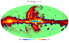
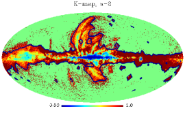
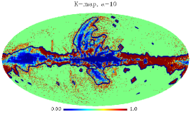
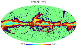
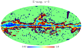
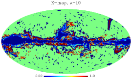
Figure 2: Upper: the $\mathbf{k}(a,P_{t})$ maps in comparison to PAM (dark blue contour line), where $\mathbf{k}(a,P_{t})$ is generated from the WMAP 23 GHz band polarization intensity map with the same sky fraction ($\mathbf{k}=1$) as PAM, and the ranks are 1, 2 and 10 (from left to right). Lower: similar to the upper panels but for the Planck 353 GHz band polarization intensity map and CSM. Note that for better visibility, the area equal to 1 in both the $\mathbf{k}(a,P_{t})$ map and the PAM/CSM masks is set to green.

As is evident from Figure 2, the regions where $\mathbf{k}(a,P_{t})=1$ have approximately the same morphology as the corresponding WMAP/Planck masks, but there are also some different features that are noteworthy. Firstly, outside PAM, one can see a few extended arches that are not masked out by PAM, which does not change significantly with different choices of $a$, while inside the mask the corresponding shape of the filter critically depends on rank $a$. Variation of $a$ from 1 to 10 makes the inner zone approach zero, in agreement with Figure 1.

Another feature of the P-filter is clearly visible along the Galactic plane at the galactic longitudes $180^{\circ}\leq\textbf{l}\leq 300^{\circ}$ (right hand side): For PAM, this zone is indiscriminately removed from analysis, while with a P-filter, there is no strong suppression in this area ($\mathbf{k}\approx 1$), because the polarization intensities here are not much higher than the threshold $P_{t}$. Meanwhile, we can see many red dots outside the PAM, which are not included in the PAM because, to reduce discontinuity, it is not preferable to keep too many tiny holes in a top-hat mask. However, for the P-filter family this is not a problem, because the filter function is always continuous.

By comparing the upper and lower panels of Figure 2, we see that, for the Galactic plane region at $180^{\circ}\leq\textbf{l}\leq 300^{\circ}$, the two top-hat masks (PAM and CSM) are similar, but the corresponding P-filters are able to show more differences between 23 and 353 GHz: the P-filter based on 23 GHz gives less suppression in this region than the one based on 353 GHz. Thus the P-filters automatically trace different map signals and give more dedicated responses than top-hat masking. Also notice that, in full sky, PAM and CSM are morphologically different, which means the design of a common mask for multi-frequency analysis of the CMB foregrounds and cosmological products need more investigations.

We also point out that the P-filter can be applied to both temperature and polarization maps. An example for the temperature map can be found in Appendix B, which is similar to Figure 2.

3 Common P-filter for multiple frequency bands

3.1 Variation of the P-filter threshold

We argue here that, one cannot use the same P-filter threshold for two different frequency bands, if they contain different foregrounds. To illustrate this issue, we take under consideration the WMAP 23–94 and Planck 30–353 GHz bands (at $N_{side}=128$), and construct histograms of the corresponding polarization intensity maps (before P-filtering). Some of these histograms are shown in the top panel of Figure 3. They help to illustrate how the threshold $P_{t}$ for each frequency band should be determined differently. Taking the Planck 353 GHz band for example, in Table 1 we present the values of $P_{t}$ that gives the corresponding sky fraction $f_{sky}$. The vertical line shows $P_{t}=56$ $\mu$K corresponding to $f_{sky}=0.5$ from 353 GHz map. For K-band this threshold removes roughly same amount of pixels, while for 70 and 143 GHz maps only a small fraction of the pixels can exceed $P_{t}=56$ $\mu$K.

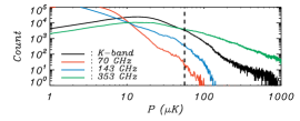
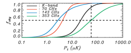
Figure 3: Illustrations of the relationship between $P_{t}$ and frequency bands. Left: Histograms of the polarization intensities for some example frequency bands, where the vertical line marks 56 $\mu$K for example. Middle: fraction of the sky ($f_{sky}$) with $P<P_{t}$ as function of $P_{t}$, the vertical line is the same as in the top panel, and the horizontal line marks the 50$\%$ position. Right: The median polarization intensity within the Planck union mask VS. the frequency bands. The two red points are the WMAP V and W bands.

Table 1: The sky fraction of $\mathbf{k}=1$ for the 353 GHz polarization intensity map with a given threshold $P_{t}$.

$f_{sky}$, $\%$	50	60	70	80
$P_{t}$, $\mu$K	56	80	116	183

The middle panel of Figure 3 shows the dependency of the sky fraction $f_{sky}$ on $P_{t}$ for the same bands in the left panel. From this panel one can see that, for instance, keeping $f_{sky}\simeq 0.5$ requires $P_{t}\simeq 2-5$ $\mu$K for 70 and 143 GHz, and $P_{t}\simeq 20$ $\mu$K for the K band. The bottom panel of Figure 3 illustrates the median polarization intensities of the region covered by an example mask (Planck 2015 Union mask) for all the frequency bands, which also show the tendency of polarization intensity variation in the given region versus frequencies.

3.2 Construction of a common P-filter

We see from above that the P-filter should be different for different frequency bands. However, it is still possible to generate a common P-filter for all frequency bands.

Primarily, to determine the P-filter for all bands, one needs $2N_{band}$ free parameters. However, we can reduce this number to only 1 as follows: We first set $f_{sky}=0.8$ for all frequency bands as a possible variant (one is free to choose another value based on any specific requirement). As we have shown in the previous section, the fraction $f_{sky}$ will determine the thresholds $P^{(i)}_{t}$, and with the corresponding ranks $a^{(i)}_{max}$ determined by Eq. 2.6, one can fully determine the P-filter for all bands with only 1 free parameter: $f_{sky}=0.8$. For convenience, we list all $2N_{band}$ parameters generated from $f_{sky}=0.8$ in Table 2. One can see that for all sky maps the ranks $a$ are close to 1.25, with some small variations like $a=1.33$ for 143 GHz and 1.29 for 353 GHz.

Table 2: The filter parameters used in Section 3.2, which are all correspond to the sky fraction $f_{sky}=80\%$. The unit for $P_{t}$ is $\mu$K.

Band	K	30	Ka	Q	44	V
$P_{t}$	42	20	17	13	9	12
$a$	1.21	1.22	1.21	1.22	1.22	1.27
Band	70	W	100	143	217	353
$P_{t}$	6	16	4	7	23	180
$a$	1.24	1.38	1.26	1.33	1.29	1.29

Based on Table 2, we can define a common filter $\mathbf{K}$ as the multiplication of all 12 $\mathbf{k}_{i}$ (other combinations are also possible) maps as

$$\mathbf{K}=\prod^{N}_{i=1}\mathbf{k}_{i},$$ (3.1)

which is shown in Figure 4. Similarly, we can also define the common filter using only the Planck bands or only the lowest and highest bands (23 and 353 GHz), which are all shown in the same figure.

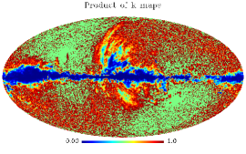
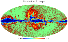
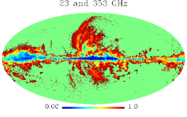
Figure 4: The $K(\textbf{n})$ maps produced from Table 2. Left: for all 12 bands. Middle: for only the Planck frequency bands. Right: for only the 23 and 353 GHz (synchrotron and dust), which is the one to be used in this work. The region where $k(\mathbf{n})=1$ is marked in green for visibility.

The combination of all 12 bands gives a very aggressive common P-filter, which can be used for the most conservative purposes. A curious feature of the $\mathbf{K}$-map that includes the WMAP bands is the presence of the instrumental noise, clearly seen along the Ecliptic plane zone as red dots. Nevertheless, the amplitudes of the $\mathbf{K}$-map in those dots are close to 1 (which still ensures continuity). The $\mathbf{K}$-map for Planck bands alone is less noisy, but it still reveals some features of the synchrotron and thermal dust well outside the Galactic plane, associated with galactic Loop I and arches [13]. As it is seen from Figure 4, the effective common P-filter for Planck data alone is significantly different in respect to the CSM. It is less aggressive than CSM in the Galactic plane zone, but more aggressive in the Loop I and surrounding zones. Recall that, the common P-filter is not fixed: it can vary according to the combination of frequency bands included in Eq. 3.1. Moreover, for the forthcoming CMB experiments the particular shape of the common filter will be based on the new data, keeping in mind, however, the recipe of its construction here and some peculiarities of the filter to be listed below.

Below in Section 4, we will work with a simplified case and use the $\mathbf{K}$-map produced only from the lowest and highest bands (23 and 353 GHz), shown in the right panel of Figure 4. This can reflect the basic properties of the synchrotron and dust polarizations and is least affected by the instrumental noise in the polarized foregrounds.

4 Advantages of a common P-filter

As mentioned above, in this section we use the simplified common P-filter in the right panel of Figure 4 for testing purposes.

4.1 Automatic removal of the strong point sources

If the amplitude of a point source exceeds the threshold $P_{t}$ for some of the frequency band maps included in the $K(\textbf{n})$ map, it will be automatically removed by the P-filter for all the maps without any extra cost and without losing continuity.

For example, with the common P-filter mentioned above (which makes no additional requirements on the method of point source removal), the polarized strong point sources in the WMAP K-band map around $(\textbf{l},\textbf{b})=(309^{\circ},20^{\circ})$ are automatically removed, as shown in Figure 5. Note that the removal will still maintain continuity of the signal in the map, and obviously a better and more thorough point source removal can be done by adjusting the filter parameters for a specific band and a specific local region.

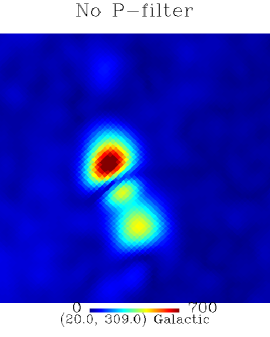
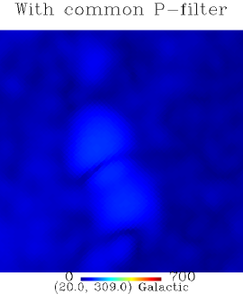
Figure 5: Example of how the common P-filter automatically and smoothly removes a polarized point source in the WMAP K-band map around $(\textbf{l},\textbf{b})=(309^{\circ},20^{\circ})$, without any special design. The map unit is $\mu$K (same for the rest sky maps).

4.2 Reducing the leakage associated with bandpass

In Fourier analysis, it is well known that when a localized signal is cut off in the frequency domain, it will no longer be localized anymore, but instead will start to leak into other regions in the pixel domain, even those far away from the source. In the analysis of a sky map, a similar problem also exists: when a sky map is bandpassed in the harmonic space, the high amplitude signal from the brightest pixels will start to leak into other regions and produce unwanted contamination.

There are several ways to alleviate this kind of leakage due to bandpassing, from simply using a top-hat mask, to harmonic space apodization (see for example [14]) or wavelets (see for example [15]). However, these techniques can exhibit some problems. For example, masking is the simplest solution, but it will generate further Gibbs-like effects, and it will cause other problems like power spectrum leakage [16] and EB-leakage [12, 17, 18, 19, 20]. Harmonic space apodization will inevitably keep some unwanted multipole components; meanwhile, there are countless schemes for apodization, which makes it difficult to make a “natural” choice. Wavelets are computationally expensive, and they do not have straightforward mapping to a single spherical harmonic component.

The P-filter provides an easy, quick and cheap way to prevent the leakages right from the pixel domain. To provide an example, in Figure 6, we show the effect of the above mentioned common P-filter in combination with a simple bandpass from $L=60$ to $L=100$ on the 353 GHz polarization map (P-filtering first, then bandpassing). One can see that, without the P-filter, the bandpass will cause serious stripe-like leakages, but after applying the common P-filter introduced in the end of Section 3.2, the leakage is largely eliminated. This example can be further improved by optimizing the common P-filter based on more specific requirements.

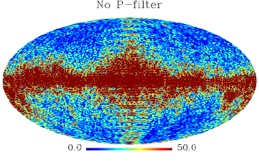
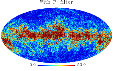
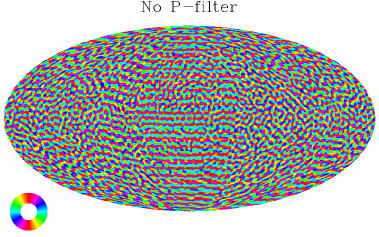
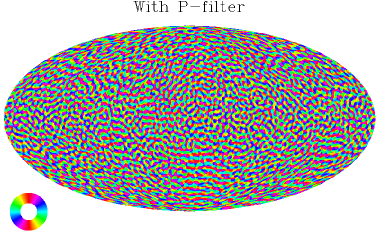
Figure 6: Results of bandpassing the Planck 353 GHz polarization map from $L=60$ to $L=100$ without/with (left/right) the common P-filter in advance. Upper: polarization intensities. Lower: polarization angles.

4.3 Reducing the EE, BB leakages

A full sky polarization map can be decomposed into $(Q_{E},U_{E})$ and $(Q_{B},U_{B})$ families of Stokes parameters that come only from the E or B modes respectively. This decomposition satisfies

$$(Q,U)\equiv(Q_{E},U_{E})+(Q_{B},U_{B}),$$ (4.1)

where $(Q,U)$ are the input Stokes parameter maps. More details can be found in Appendix A and [21, 22].

If a polarized sky map is decomposed into E and B families (or traditional E and B modes) without a P-filter, then there is going to be cross-talk between different regions of the sky, even if one uses a full sky map from the beginning. The reason is that, very bright regions (like the Galactic plane) will produce many extended pixel domain $(Q_{E},U_{E})$ and $(Q_{B},U_{B})$ family components, which are pure contamination for other regions. Note that this phenomenon is unique for polarization, and does not exist for a temperature map, except for some small residuals due to the pixelization and $L_{max}$ limitation. One important advantage of the P-filter is to reduce such EE and BB leakages in estimating the full sky $(Q_{E},U_{E})$ and $(Q_{B},U_{B})$ families. The reason is easy to understand: the brightest pixels will be significantly suppressed by the P-filter in a continuous way,

In Figure 7, we present straightforward comparisons of decomposing the full-sky Planck 353 GHz polarization map into the $(Q_{E},U_{E})$ and $(Q_{B},U_{B})$ families with and without the common P-filter mentioned above. The prevention of leakage can be easy observed by much cleaner results at higher latitudes.

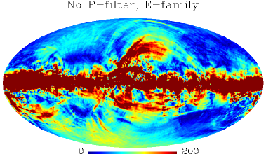
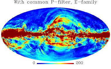
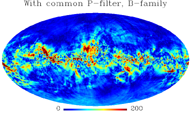
Figure 7: Full sky E/B family components (upper/lower) derived from the Planck 353 GHz map before/after (left/right) applying the common P-filter.

4.4 Reducing the EB-leakage

Formally speaking, calculation and separation of the E and B families (Eq. 4.1) should be done on the full sky. If part of the sky is missing, the two families will be mixed and create E-to-B and B-to-E leakage in the available sky region. For CMB science, one is mainly interested in the E-to-B leakage, because the B-mode of CMB is related to the primordial gravitational waves.

If, from the very beginning, only part of the sky is available, then the E-to-B leakage cannot be precisely estimated. However, we can construct tests using full-sky foreground maps as known inputs to simulate and evaluate the E-to-B leakage. Here we perform such a test using the P-filter.

We take the WMAP K-band full-sky synchrotron polarization maps and separate them into E- and B-families as described in Appendix A. Then we apply a top-hat mask to the E-family and redo the EB-separation. The difference between the resulting B-family in the available sky region and the known real B-family is exactly the E-to-B leakage due to the top-hat masking. We then repeat the procedure using the common P-filter instead of a top-hat mask and compare the results in Figure 8. We can see that, without any correction, the P-filter gives much lower E-to-B leakage than the top-hat mask. Similar tests are done for the Planck 353 GHz map, giving similar results as shown in the same figure. Therefore, although a top-hat mask completely kills all foreground in the “unwanted” region, a P-filter with moderate suppression will actually give much lower E-to-B leakage and a better B-mode in the “desired” region. We use a top-hat mask as a reference here and below to show that the P-filter does not suffer from the same problems related to the top-hat masking. Comparisons to more realistic masking techniques used in CMB analysis, such as masks with smoothed boundaries, will be given in a future paper.

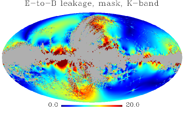
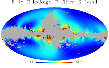
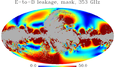
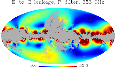
Figure 8: Examples showing how a common P-filter helps to alleviate the E-to-B leakage (without further correction). Upper: K-band. Lower: 353 GHz. Left: with a top-hat mask. Right: with a P-filter.

4.5 Reducing the EB-leakage for a CMB map

When the P-filter is applied to a band map, not only the foregrounds, but also the underlying CMB signal will be multiplied by the common $\mathbf{K}$-map. This could potentially change the polarization angles of the $(Q_{E},U_{E})$ and $(Q_{B},U_{B})$ families, which are defined as

$$\theta_{E} =0.5\mathbf{arctan2}(U_{E},Q_{E}),$$ (4.2)

$$\theta_{B} =0.5\mathbf{arctan2}(U_{B},Q_{B}),$$

where $\mathbf{arctan2}$ is an extension of the $\mathbf{arctan}$ function that returns results in the range $(0,2\pi)$. Here we check the extent to which $\theta_{E}$ and $\theta_{B}$ might change due to the P-filter. We generate a simulated CMB map, filter it with the common P-filter, and bandpass to $\ell=60$–100. Then we extract the polarization angles $\theta_{E}^{\prime}$ and $\theta_{B}^{\prime}$ in interior of the region with $\mathbf{K}=1$, where we discard the edges by excluding a 3-pixel width contour (at $N_{side}=512$) along the edge of the mask. Then we compute the following quantities to compare the angles of the filtered map with those of the real CMB, (denoted by $\theta_{E}$ and $\theta_{B}$):

$$\Delta\theta_{E} =|\arcsin(\theta^{\prime}_{E}-\theta_{E})|,$$ (4.3)

$$\Delta\theta_{B} =|\arcsin(\theta^{\prime}_{B}-\theta_{B})|,$$

where $\theta^{\prime}_{E}$ and $\theta^{\prime}_{B}$ are the polarization angles after filtering. Note that because the change $\Delta\theta_{B}$ is dominated by the E-to-B leakage, this test shows the extent to which the P-filter helps to alleviate the E-to-B leakage problem.

We calculate the histogram of the changes of $\Delta\theta_{E}$ and $\Delta\theta_{B}$ and plot them in Figure 9. We also calculate the mean polarization angle changes, which are only $1.0^{\circ}$ for no separation and $\Delta\theta_{E}$, and only $3.0^{\circ}$ for $\Delta\theta_{B}$, compared to $5.5^{\circ}$ and $17^{\circ}$ respectively for the case with a top-hat mask. Therefore, with a P-filter, the variation of the polarization angle is significantly reduced in comparison to using a top-hat mask.

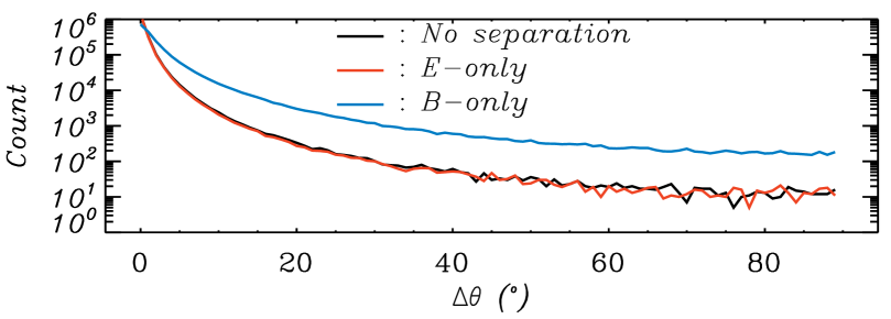
Figure 9: Histogram of the polarization angle differences after the pixel domain filtering using the common P-filter and band passing for $L=60$–$100$, for no separation, $\Delta\theta_{E}$ and $\Delta\theta_{B}$ respectively. The mean polarization angle variations are $1.0^{\circ}(5.5^{\circ})$ for no separation and $\Delta\theta_{E}$, and is $3.0^{\circ}(17^{\circ})$ for $\Delta\theta_{B}$, where the values in brackets are for the reference case with a top-hat mask.

5 Example of optimizing the filter parameter

Here we discuss a more practical situation, where we shall apply the P-filter on a CMB+foreground map directly (without foreground removal), and try to optimize the filter to suppress the leakage of foreground and obtain a CMB B-mode signal that is as reliable as possible in the sky region of interest. Especially, since the P-filters are smooth and continuous, we expect it to give much less E-to-B leakage in the region of interest. Note that for faster optimization, we use $N_{side}=128$ in this section. Also note that here we allow the filter parameters to be variables, so we are not dealing with the common P-filter in Section 3 anymore. Finally, since we are studying the P-filter in this work, we do not use any other correction methods.

A detailed description of the processes is as follows:

1. We generate a test foreground that has a belt shape along the Galactic plane, which decays exponentially at higher latitudes with FWHM = $20^{\circ}$. The central polarization intensity is 4000 $\mu$K, and the polarization angles are randomly and uniformly distributed. The test foreground is shown in the upper-left panel of Figure 10.

2. We generate a simulated CMB map with $r=0.05$, and use the CMB+foreground map as the input of the P-filter. Note that the real CMB map will not be used anymore until the final comparison.

3. We take a “region of interest” that has $|\textbf{b}|>45^{\circ}$, to simulate using high Galactic latitude region. This “region of interest” is only used for comparison of the final results, and one can see later from Figure 10 that the comparison is not sensitive to the size of this region.

4. We try several P-filters with various threshold $P_{t}$ and rank $a$ on the CMB+foreground map, and for each set of $(P_{t},a)$, we calculate the filtered B-mode polarization intensity ($\mathbf{P}_{B}=\sqrt{\mathbf{Q}_{B}^{2}+\mathbf{U}_{B}^{2}}$) from the full sky, and then calculate the average polarization intensity $\langle P_{B}\rangle=\sqrt{\langle\mathbf{P}_{B}^{2}\rangle}$ only in the “region of interest”. The best threshold and rank are determined by minimizing $\langle P_{B}\rangle$. The results are $P_{t}=1.15$ $\mu$K and $a=3$. Note that this step does not require to know the input CMB or foreground, and the optial parameters are specific to the simulated foreground in use.

5. With $P_{t}$=$1.15$ $\mu$K and $a=3$, we filter the CMB+foreground map, and derive $P_{B}$ from the filtered full sky map in the multipole range from $L=60$ to $L=100$. Then we subtract the known CMB $P_{B}$ from the filtered $P_{B}$, and show the difference in the lower-left panel of Figure 10. Note that the region with $\mathbf{k}\neq 1$ is the region in which the P-filter really works, which is called the “working region”. The “working region” is also shown in the upper right panel of the same figure.

6. We use the same threshold $P_{t}$ but infinite rank $a$ to repeat step 5, which represents the performance of a top-hat mask. The corresponding $\mathbf{P}_{B}$ map difference is presented in the lower-right panel of Figure 10.

Except for the final comparison of the $\mathbf{P}_{B}$ map, the above procedure depends only on the combined CMB+foreground map. From Figure 10, we can see that, a P-filter can significantly suppress the leakage due to the foreground and output a B-mode polarization intensity very similar to the real input in the “region of interest”. On the other hand, a top-hat mask certainly kills the foreground more thoroughly, but the price is to leave much more leakage in the whole “region of interest”, which is not preferable.

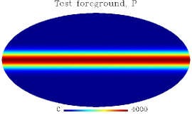
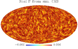
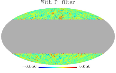
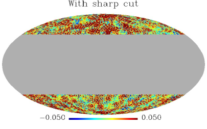
Figure 10: Upper, from left to right: polarization intensity of the input test foreground, real $\mathbf{P}_{B}$ map from the input CMB map in multipole range $L=60$–$100$, and illustration of the common working region of the P-filter (green). Lower left: the map of $P_{B}$ difference, computed as $\mathbf{P}_{B}-\mathbf{P}_{B}^{real}$ in the multipole range $L=60$–$100$. Lower right: same as the lower-left panel, only that top-hat masking is used instead of the P-filter. The “region of interest” is the non-gray region in the lower panels. See Section 5 for more details.

6 Discussion

In this work, we design the P-filter, which succeeds the basic idea of masking in CMB science to “remove the brightest pixels”. Instead of top-hat masking, the P-filter works in a smooth and continuous way, with simple and clear mathematical definition.

The P-filters help to greatly simply the task to design a mask for analysis: For a top hat mask, one has to pay extra attention to the serrated edge and the individual tiny holes, and, to fix them, one often need some arbitrary choice. However, for a P-filter, the serrated edge and the individual tiny holes are not a problem at all, and the filter can be designed with just one parameter. It is also much easier to use P-filter than to use a top-hat mask when working with multiple resolutions, because for a top-hat mask, changing its resolution is often problematic, but a P-filter can be conveniently regenerated at a new resolution using the same set of parameter(s).

The pixel domain form of the P-filter is same as a pixel domain window function/apodization, but they have completely different idea of design. A normal pixel domain window function is defined on independent variables like sky coordinates $(\theta,\phi)$, or time $t$ (for a time series). However, the P-filter is defined directly on dependent variable like polarization intensity or temperature. This is why the P-filter is independent to the coordinate system, and is able to trace the map morphologies automatically.

The idea to work on dependent variables also brings two other advantages on continuity and gradient. Firstly, we know that real maps have to be presented with a finite resolution, thus all window functions defined on the coordinate system (independent variables) will be affected and will bring extra discontinuity depending on the way they are defined (although this effect is normally small). However, the P-filter is defined on the dependent variables, thus it will not bring extra discontinuity due to pixelization. Secondly, window functions defined on independent variables can either increase or decrease the gradient, however, a P-filter will always help suppress the high gradients due to strong foregrounds, which is convenient.

We show in this work that the P-filter family can effectively reduce many leakage problems, including the ones associated with bandpassing and EB-separation. It can also be used to naturally suppress the regions with residual contamination in CMB products or a partial sky map, for example, removal of bright point sources. However, we point out that the P-filter can not resolve the problem of peculiar zones of the maps, especially the ones related to the systematic effects, which should always be treated separately for safety.

The P-filter family has a well-defined semi-analytic form. As shown in Section 3, when applied to multiple frequency bands to create a common P-filter, it is possible to reduce the number of free parameters to only 1, which is the $f_{sky}$ with $\mathbf{k}(a,P_{t})=1$. Note that this is exactly the parameter that represents the basic idea of masking in CMB science.

The family of P-filters also provides a mathematical means to move smoothly from the case of no filtering to the case of top-hap masking, by continuously changing the rank parameter $a$ from 0 to $\infty$, as illustrated in Figure 1. For each intermediate step in the movement, continuity of the filter is always preserved to the first derivative. This provides an excellent way to find a balance between removing more contaminated pixels and keeping more continuity by optimizing the threshold $P_{t}$ and the rank $a$, as shown by the example in Section 5. Mathematically, this also provides a progressive way to study the properties of top-hat masking by letting $a$ approach infinite, which might be interesting.

Appendix A The definition of EB-families

In our work, the E and B families refers to $(Q_{E},U_{E})$ and $(Q_{B},U_{B})$ that contain only E or B mode respectively, and satisfy $(Q,U)\equiv(Q_{E},U_{E})+(Q_{B},U_{B})$. They are defined as follows:

$$\begin{split}\begin{pmatrix}Q_{E}\\ U_{E}\end{pmatrix}(\bm{n})&=\int\begin{pmatrix}G_{1}&+G_{2}\\ +G_{3}&G_{4}\end{pmatrix}(\bm{n},\bm{n}^{\prime})\begin{pmatrix}Q\\ U\end{pmatrix}(\bm{n}^{\prime})\,d\bm{n}^{\prime}\\ \begin{pmatrix}Q_{B}\\ U_{B}\end{pmatrix}(\bm{n})&=\int\begin{pmatrix}G_{4}&-G_{3}\\ -G_{2}&G_{1}\end{pmatrix}(\bm{n},\bm{n}^{\prime})\begin{pmatrix}Q\\ U\end{pmatrix}(\bm{n}^{\prime})\,d\bm{n}^{\prime},\end{split}$$ (A.1)

where the $G_{1-4}$ functions are defined as:

$$\begin{split}G_{1}(\bm{n},\bm{n}^{\prime})&=\sum_{l,m}F_{+,\ell m}(\bm{n})F^{*}_{+,\ell m}(\bm{n}^{\prime}),\\ \quad G_{2}(\bm{n},\bm{n}^{\prime})&=\sum_{l,m}F_{+,\ell m}(\bm{n})F^{*}_{-,\ell m}(\bm{n}^{\prime}),\\ G_{3}(\bm{n},\bm{n}^{\prime})&=\sum_{l,m}F_{-,\ell m}(\bm{n})F^{*}_{+,\ell m}(\bm{n}^{\prime}),\\ \quad G_{4}(\bm{n},\bm{n}^{\prime})&=\sum_{l,m}F_{-,\ell m}(\bm{n})F^{*}_{-,\ell m}(\bm{n}^{\prime}),\end{split}$$ (A.2)

and the $F_{+,-}$ functions are defined in terms of the spin-2 spherical harmonics as:

$$\begin{split}F_{+,\ell m}(\bm{n})&=-\frac{1}{2}\left[{}_{2}Y_{\ell m}(\bm{n})+{}_{-2}Y_{\ell m}(\bm{n})\right],\\ F_{-,\ell m}(\bm{n})&=-\frac{1}{2i}\left[{}_{2}Y_{\ell m}(\bm{n})-{}_{-2}Y_{\ell m}(\bm{n})\right].\end{split}$$ (A.3)

Note that $G_{i}$ are real and $G_{2}=G_{3}$. For more details of these two families, see [21, 22].

Appendix B Example of P-filter for a temperature map

In Figure 2, we already see examples that the P-filter can naturally provide the same sky coverage and similar morphology to existing WMAP and Planck polarization masks. We also provide examples of generating P-filters based on the Planck 353 GHz temperature (not polarization) maps, and compare the results to the Planck power spectrum analysis masks. For those masks, Planck provides 8 different sky coverage with $f_{sky}=$0.2, 0.4, 0.6, 0.7, 0.8, 0.9, 0.97, and 0.99 respectively. For convenience, we take only $f_{sky}=$0.2, 0.4, 0.6, and 0.8 to generate the corresponding variants of the P-filters, and the polarization intensity P is replaced by the temperature, $T$, and the threshold $P_{t}$ by $T_{t}$. In this paragraph, we focus on the effect the threshold has, thus we keep using the same rank $a=1$. In Figure 11 we compare the derived $\mathbf{k}$ maps to the Planck masks in a similar way to Figure 2, where one can see that for either case (30 or 353 GHz), the generated $\mathbf{k}$ maps have similar morphologies to the Planck masks with the same $f_{sky}$. This tells us that the P-filters can easily serve as an alternative of the masks used by WMAP and Planck to suppress the foreground or residual foreground, and at the same time, automatically provide apodizations that are continuous to the first derivative everywhere.

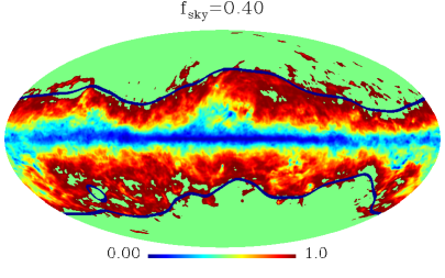
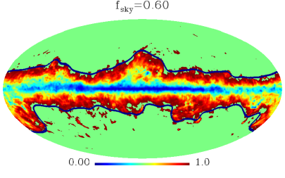
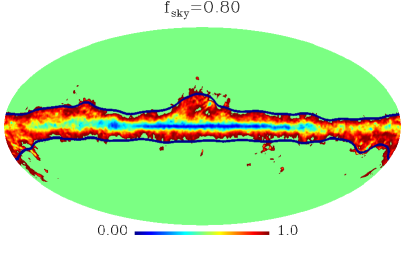
Figure 11: The $\mathbf{k}$ maps generated from the Planck 353 GHz temperature maps with $f_{sky}=0.2,0.4,0.6$, and $0.8$ (upper left to lower right), in comparison to the Planck power spectrum analysis masks with the same $f_{sky}$ (blue contour lines).

References

- [1] Planck Collaboration, P. A. R. Ade, N. Aghanim, M. I. R. Alves, C. Armitage-Caplan, M. Arnaud et al., Planck 2013 results. I. Overview of products and scientific results, Astr. Astrophys. 571 (Nov., 2014) A1, [1303.5062].
- [2] Planck Collaboration, R. Adam, P. A. R. Ade, N. Aghanim, Y. Akrami, M. I. R. Alves et al., Planck 2015 results. I. Overview of products and scientific results, Astr. Astrophys. 594 (Sept., 2016) A1, [1502.01582].
- [3] Planck Collaboration, Y. Akrami, F. Arroja, M. Ashdown, J. Aumont, C. Baccigalupi et al., Planck 2018 results. I. Overview and the cosmological legacy of Planck, ArXiv e-prints (July, 2018) , [1807.06205].
- [4] M. Hazumi, J. Borrill, Y. Chinone, M. A. Dobbs, H. Fuke, A. Ghribi et al., LiteBIRD: a small satellite for the study of B-mode polarization and inflation from cosmic background radiation detection, in Space Telescopes and Instrumentation 2012: Optical, Infrared, and Millimeter Wave, vol. 8442 of Proc. SPIE, p. 844219, Sept., 2012, DOI.
- [5] K. N. Abazajian, P. Adshead, Z. Ahmed, S. W. Allen, D. Alonso, K. S. Arnold et al., CMB-S4 Science Book, First Edition, ArXiv e-prints (Oct., 2016) , [1610.02743].
- [6] B. Keating, S. Moyerman, D. Boettger, J. Edwards, G. Fuller, F. Matsuda et al., Ultra High Energy Cosmology with POLARBEAR, ArXiv e-prints (Oct., 2011) , [1110.2101].
- [7] J. A. Rubiño-Martín, R. Rebolo, M. Aguiar, R. Génova-Santos, F. Gómez-Reñasco, J. M. Herreros et al., The quijote-cmb experiment: studying the polarisation of the galactic and cosmological microwave emissions, Proc.SPIE 8444 (2012) 8444 – 8444 – 11.
- [8] M. Zaldarriaga and U. c. v. Seljak, All-sky analysis of polarization in the microwave background, Phys. Rev. D 55 (Feb, 1997) 1830–1840.
- [9] M. Zaldarriaga, Cosmic microwave background polarization experiments, The Astrophysical Journal 503 (1998) 1.
- [10] BICEP2/Keck Collaboration, Planck Collaboration, P. A. R. Ade, N. Aghanim, Z. Ahmed, R. W. Aikin et al., Joint Analysis of BICEP2/Keck Array and Planck Data, Physical Review Letters 114 (Mar., 2015) 101301, [1502.00612].
- [11] C. L. Bennett, R. S. Hill, G. Hinshaw, M. R. Nolta, N. Odegard, L. Page et al., First-Year Wilkinson Microwave Anisotropy Probe (WMAP) Observations: Foreground Emission, Astrophys. J.Suppl. 148 (Sept., 2003) 97–117, [astro-ph/0302208].
- [12] K. M. Smith, Pseudo-Cℓ estimators which do not mix E and B modes, Phys. Rev. D 74 (Oct., 2006) 083002, [astro-ph/0511629].
- [13] M. Vidal, C. Dickinson, R. D. Davies and J. P. Leahy, Polarized radio filaments outside the Galactic plane, Mon. Not. R. Astr. Soc. 452 (Sept., 2015) 656–675, [1410.4438].
- [14] Planck Collaboration, R. Adam, P. A. R. Ade, N. Aghanim, M. Arnaud, M. Ashdown et al., Planck 2015 results. IX. Diffuse component separation: CMB maps, Astr. Astrophys. 594 (Sept., 2016) A9, [1502.05956].
- [15] S. Basak and J. Delabrouille, A needlet internal linear combination analysis of WMAP 7-year data: estimation of CMB temperature map and power spectrum, Mon. Not. R. Astr. Soc. 419 (Jan., 2012) 1163–1175, [1106.5383].
- [16] E. Hivon, K. M. Górski, C. B. Netterfield, B. P. Crill, S. Prunet and F. Hansen, MASTER of the Cosmic Microwave Background Anisotropy Power Spectrum: A Fast Method for Statistical Analysis of Large and Complex Cosmic Microwave Background Data Sets, Astrophys. J. 567 (Mar., 2002) 2–17, [astro-ph/0105302].
- [17] J. Kim and P. Naselsky, E/B decomposition of CMB polarization pattern of incomplete sky: a pixel space approach, Astr. Astrophys. 519 (Sept., 2010) A104, [1003.2911].
- [18] W. Zhao and D. Baskaran, Separating and types of polarization on an incomplete sky, Phys. Rev. D 82 (Jul, 2010) 023001.
- [19] E. F. Bunn and B. Wandelt, Pure E and B polarization maps via Wiener filtering, Phys. Rev. D 96 (Aug., 2017) 043523, [1610.03345].
- [20] D. Kodi Ramanah, G. Lavaux and B. D. Wandelt, Optimal and fast E/B separation with a dual messenger field, ArXiv e-prints (Jan., 2018) , [1801.05358].
- [21] H. Liu, J. Creswell and P. Naselsky, E and B families of the Stokes parameters in the polarized synchrotron and thermal dust foregrounds, JCAP 5 (May, 2018) 059, [1804.10382].
- [22] H. Liu, Fingerprint of Galactic Loop I on polarized microwave foregrounds, Astr. Astrophys. 617 (Sept., 2018) A90, [1806.06532].
- [23] The WMAP data release. https://lambda.gsfc.nasa.gov/product/map/dr5/, 2013.
- [24] The Planck data release. https://www.cosmos.esa.int/web/planck/pla, 2018.
- [25] K. M. Górski, E. Hivon, A. J. Banday, B. D. Wandelt, F. K. Hansen, M. Reinecke et al., HEALPix: A Framework for High-Resolution Discretization and Fast Analysis of Data Distributed on the Sphere, Astrophys. J. 622 (Apr., 2005) 759–771, [astro-ph/0409513].