Evaporating black-holes, wormholes, and vacuum polarisation:
must they always conserve charge?

Abstract

A careful examination of the fundamentals of electromagnetic theory shows that due to the underlying mathematical assumptions required for Stokes’ Theorem, global charge conservation cannot be guaranteed in topologically non-trivial spacetimes. However, in order to break the charge conservation mechanism we must also allow the electromagnetic excitation fields D, H to possess a gauge freedom, just as the electromagnetic scalar and vector potentials $\varphi$ and A do. This has implications for the treatment of electromagnetism in spacetimes where black holes both form and then evaporate, as well as extending the possibilities for treating vacuum polarisation. Using this gauge freedom of D, H we also propose an alternative to the accepted notion that a charge passing through a wormhole necessarily leads to an additional (effective) charge on the wormhole’s mouth.

There is a popular summary at the end: VIII.

I Introduction

It is not only a well established, but an extremely useful consequence of Maxwell’s equations, that charge is conserved Jackson-ClassicalED . However, this principle relies on some assumptions, in particular those about the topology of the underlying spacetime, which are required for Stokes’ Theorem to hold. Here we describe how to challenge the status of global charge conservation, whilst still keeping local charge conservation intact. We do this by investigating the interaction of electromagnetic theory and the spacetime it inhabits, and go on to discuss the potential consequences of such a scenario.

As well as considering topologically non-trivial spacetimes, we also no longer demand that the excitation fields D, H are directly measurable. This relaxation means that the excitation fields D, H are now allowed a gauge freedom analogous to that of the scalar and vector electromagnetic potentials $\varphi$ and A. This gauge freedom for D, H is given by

$$\textbf{D}\rightarrow\textbf{D}+\nabla\times\textbf{A}_{\textup{g}},\quad \textbf{H}\rightarrow\textbf{H}+\dot{\textbf{A}}_{\textup{g}}+\nabla\varphi_{\textup{g}},$$ (1)

where $\varphi_{\textup{g}}$ and $\textbf{A}_{\textup{g}}$ are the new gauge terms, which vanish when inserted into Maxwell’s equations. Note that there are already long-standing debates about whether – or how – any measurement of the excitation fields might be done (see e.g. Heras-2011ajp ; Gratus-KM-2019ejp-dhfield and references therein). Unlike the case for E, B, there is no native Lorentz force-like equation for magnetic monopoles dependent on D, H, although proposals – based on the assumption that monoples indeed exist – have been discussed Rindler-1989ajp . Neither is there an analogous scheme for measuring E, B inside a disk by using the Aharonov-Bohm effect Ehrenberg-S-1949prsb ; Aharonov-B-1959pr ; Matteucci-IB-2003fp , a method particularly useful inside a medium where collisions may prevent a point charge obeying the Lorentz force equation. This double lack means that whenever making claims about the measurability of D, H, one has to make assumptions about their nature, for example that it is linearly and locally related to E, B, such as in the traditional model of the vacuum. Such assumptions act to fix any gauge for D, H, so that one can measure the remaining parameters; but if D, H are taken to be not measurable, then the gauge no longer needs to be fixed.

The relaxed assumptions about topology and gauge are not merely minor technical details, since many cosmological scenarios involve a non-trivial topology. Notably, black holes have a central singularity that is missing from the host spacetime Schutz-FCRelativity ; MTW , and a forming and then fully evaporated black hole creates a non-trivial topology, which in concert with allowing a gauge freedom for now non-measureable D, H fields, breaks the usual basis for charge conservation. We also consider more exotic scenarios, such as the existence of a universe containing a wormhole (see e.g. Morris-T-1988ajp ), or a “biverse”– a universe consisting of two asymptotically flat regions connected by an Einstein-Rosen bridge. In particular we test the claim that charges passing through such constructions (wormholes) are usually considered to leave it charged Visser-LW ; Susskind-2005arXiv ; Wheeler-1957ap .

Topological considerations and their influence on the conclusions of Maxwell’s theory are not new, but our less restrictive treatment of D, H allows us a wider scope than in previous work. Misner and Wheeler, in Wheeler-1957ap developed an ambitious programme of describing all of classical physics (i.e. electromagnetism and gravity) geometrically, i.e. without including charge at all. Non-trivial topologies, such as spaces with handles, were shown to support situations where charge could be interpreted as the non-zero flux of field lines, which never actually meet, over a closed surface containing the mouth of a wormhole. Baez and Muniain BaezMunain-GFKG show that certain wormhole geometries are simply connected, so that every closed 1-form is exact. In this case charge can then be defined as an appropriate integral of the electric field over a 2-surface. In another example, Diemer and Hadley’s investigation Diemer-H-1999cqg has shown that it is possible, with careful consideration of orientations, to construct wormhole spacetimes containing topological magnetic monopoles or topological charges; and Marsh Marsh-1998jpa has discussed monopoles and gauge field in electromagnetism with reference to topology and de Rham’s theorems.

It is important to note that our investigation here is entirely distinct from and prior to any cosmic censorship conjecture Penrose-1999jaa , the boundary conditions at a singularity, models for handling the event horizon Price-T-1986prd , or other assumptions. Although an event horizon or other censorship arrangement can hide whatever topologically induced effects there might be, such issues are beyond the scope of our paper, which instead focuses on the fundamental issues – i.e. the prior and classical consequences of the violation of the prerequisites of Stokes’ Theorem in spacetimes of non-trivial topology.

In section II we summarise the features of electromagnetism relevant to our analysis. In section III we investigate under what circumstances charge conservation no longer holds, and its consequences for the electromagnetic excitation field $\bm{\mathsf{H}}$, which is the differential form version of the traditional D, H. Next, in section IV we describe further consequences, such as how a description of bound and free charges necessarily supplants a standard approach using constitutive relations based on $\bm{\mathsf{H}}$. Then, in section V we see that topological considerations mean that $\bm{\mathsf{H}}$ can be defined in a way that has implications for the measured charge of wormholes. Lastly, after some discussions in section VI, we summarise our results in section VII.

II Electromagnetism

II.1 Basics

Although perhaps the most famous version of Maxwell’s equations are Heaviside’s vector calculus form in E, B and D, H, here we instead use the language of differential forms Flanders1963 ; HehlObukhov , an approach particularly useful when treating electromagnetism in a fully spacetime context McCall-FMB-2011jo ; Gratus-KMT-2016njp-stdisp ; Cabral-L-2017fp . This more compact notation combines the separate time and space behaviour into a natively spacetime formulation, so that the four vector equations in curl and divergence are reduced to two combined Maxwell’s equations Flanders1963 ; HehlObukhov :

$${d}\bm{\mathsf{F}}=0,$$ (2)

and

$${d}\bm{\mathsf{H}}=\bm{\mathsf{J}}.$$ (3)

Here $\bm{\mathsf{F}},\bm{\mathsf{H}}\in\Gamma\Lambda^{2}\mathscr{M}$ are the Maxwell and excitation 2-form fields on spacetime $\mathscr{M}$, $\bm{\mathsf{J}}\in\Gamma\Lambda^{3}\mathscr{M}$ is the free current density 3-form, and $\Gamma$ indicates that $\bm{\mathsf{F}}$ and $\bm{\mathsf{H}}$ are smooth global sections of the bundle $\Lambda^{2}\mathscr{M}$. Conventionally, $\bm{\mathsf{F}}=\bm{\mathsf{E}}\wedge{dt}+\bm{\mathsf{B}}$, where $\bm{\mathsf{E}}$ is a 1-form representing the electric field, and $\bm{\mathsf{B}}$ is a 2-form representing the magnetic field. Taking the exterior derivative (${d}$) of (3) leads to the differential form of charge conservation, i.e. that $\bm{\mathsf{J}}$ is closed,

$${d}\bm{\mathsf{J}}=0.$$ (4)

As equations (2) and (3) are underdetermined, they need to be supplemented by a constitutive relation, connecting $\bm{\mathsf{F}}$ and $\bm{\mathsf{H}}$. In general this relation can be arbitrarily complicated, but the simplest is the “Maxwell vacuum” where they are related by the Hodge dual ${\star}$, i.e.

$$\bm{\mathsf{H}}={\star}\bm{\mathsf{F}}.$$ (5)

It is worth noting, however, that competing constitutive models exist, even for the vacuum. Two well known examples are the weak field Euler-Heisenberg constitutive relations and Bopp-Podolski Bopp-1940ap ; Podolsky-1942pr ; Gratus-PT-2015jpa constitutive relations, which are respectively

$$\bm{\mathsf{H}}_{\textup{EH}} ={\star}\bm{\mathsf{F}}-\frac{8\alpha^{2}}{45m^{4}}\left[{\star}\left(\bm{\mathsf{F}}\wedge{\star}\bm{\mathsf{F}}\right){\star}\bm{\mathsf{F}}+7{\star}\left(\bm{\mathsf{F}}\wedge\bm{\mathsf{F}}\right)\,\bm{\mathsf{F}}\right],$$ (6)

and

$$\bm{\mathsf{H}}_{\textup{BP}} ={\star}\bm{\mathsf{F}}+\ell^{2}{\star}{d}{\star}{d}{\star}\bm{\mathsf{F}},$$ (7)

where $\alpha$ is the fine structure constant, $m$ is the mass of the electron and length $\ell$ is a small parameter.

However, fixing a constitutive relation where $\bm{\mathsf{H}}$ has a straightforward relationship to $\bm{\mathsf{F}}$, such as those given above, is of itself sufficent to enforce charge conservation. In contrast, we consider more general constitutive models, and so can investigate wider possibilities.

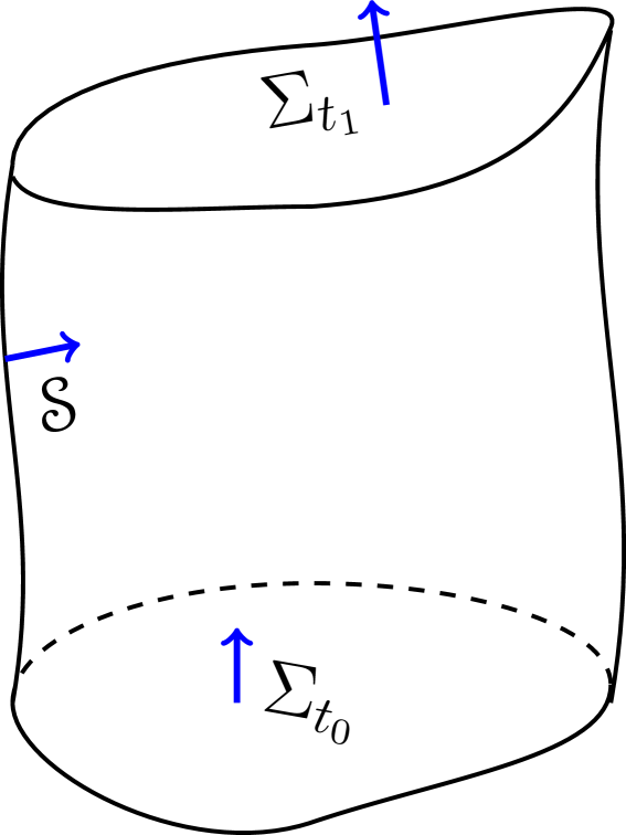
Figure 1: A closed 3-surface $\mathscr{U}$ in spacetime on which to check conservation of charge. This surface is formed from $\mathscr{U}=\mathscr{S}\bigcup{\Sigma}_{t_{0}}\bigcup{\Sigma}_{t_{1}}$, with the orientations of $\mathscr{S}$, ${\Sigma}_{t_{0}}$ and ${\Sigma}_{t_{1}}$ given by the blue arrows. Note that we do not necessarily need to consider a 4-volume enclosed by this boundary $\mathscr{U}$, as can be seen by comparing the topology condition with the gauge-free condition, as discussed in the main text.

II.2 Conservation of charge

The starting point for our investigation of topology, charge conservation, and the role of $\bm{\mathsf{H}}$, is a closed 3-surface $\mathscr{U}$ with no boundary, i.e. ${\partial}\mathscr{U}=\emptyset$. This surface $\mathscr{U}$ is topologically equivalent to the 3-sphere, and is depicted on fig. 1. We can write $\mathscr{U}=\mathscr{S}\bigcup{\Sigma}_{t_{0}}\bigcup{\Sigma}_{t_{1}}$ where ${\Sigma}_{t_{0}}$ and ${\Sigma}_{t_{1}}$ are bounded regions of the space ${\Sigma}$ at times $t_{0}$ and $t_{1}$, and $\mathscr{S}$ is the boundary of ${\Sigma}$ between the times $t_{0}\leq t\leq t_{1}$. As shown in fig. 1, the orientation of ${\Sigma}_{t_{1}}$ is outward, while those of ${\Sigma}_{t_{0}}$ and $\mathscr{S}$ are inward. Charge conservation, expressed as

$$\int_{\mathscr{U}}\bm{\mathsf{J}}=0,$$ (8)

can be expressed in this case as

$$\int_{{\Sigma}_{t_{1}}}\bm{\mathsf{J}}-\int_{{\Sigma}_{t_{0}}}\bm{\mathsf{J}}-\int_{\mathscr{S}}\bm{\mathsf{J}}=~{}~{}\int_{\mathscr{U}}\bm{\mathsf{J}}=~{}~{}0,$$ (9)

which we may interpret as the total charge in ${\Sigma}$ at time $t_{1}$ is given by the total charge in ${\Sigma}$ at time $t_{0}$, plus any charge that entered ${\Sigma}$ in the time $t_{0}\leq t\leq t_{1}$.

Irrespective of possible complications associated with the constitutive relations, charge conservation (8) follows straightforwardly in either of two ways, both due to Stokes’ theorem:

1. Topology condition: The first proof assumes that $\mathscr{U}$ is the boundary of a topologically trivial bounded region of spacetime, i.e. $\mathscr{U}={\partial}\mathscr{N}$, $\mathscr{N}\subset\mathscr{M}$, within which $\bm{\mathsf{J}}$ is defined. A topologically trivial space is one that can be shrunk to a point i.e. it is topologically equivalent to a 4-dimensional ball. Then one has

   $$\int_{\mathscr{U}}\bm{\mathsf{J}}=\int_{{\partial}\mathscr{N}}\bm{\mathsf{J}}=\int_{\mathscr{N}}{d}\bm{\mathsf{J}}=0,$$ (10)

   the last equality arising from (4), which we call the “topology condition”.

2. Gauge-free condition: The second proof arises from integrating (3) over $\mathscr{U}$, and presumes that $\bm{\mathsf{H}}$ is a well-defined 2-form field. We have that

   $$\int_{\mathscr{U}}\bm{\mathsf{J}}=\int_{\mathscr{U}}{d}\bm{\mathsf{H}}=\int_{{\partial}\mathscr{U}}\bm{\mathsf{H}}=0,$$ (11)

   where the last equality, which we call the “gauge-free condition”, results solely from the fact that $\mathscr{U}$ is closed (i.e. ${\partial}\mathscr{U}=\emptyset$), but does not require that $\mathscr{U}$ is itself the boundary of a compact 4-volume.

II.3 Non-conservation of Charge

The arguments for conservation of charge presented thus far have been mathematically rigorous. Given this sound basis, one may ask, why would anyone doubt conservation of charge? One might note, for example, the case of black holes, where charge is one of the few quantities preserved in the no-hair theorem Israel-1968cmp . However, our need to make assumptions about the nature of $\mathscr{U}$ or $\bm{\mathsf{H}}$ in the proofs (10) and (11), when establishing conservation of charge, provides us with an opportunity for testing its true basis and extent of validity. Notably, to create a charge non-conservation loophole, both (10) and (11) must be violated: if either one applies then charge is conserved.

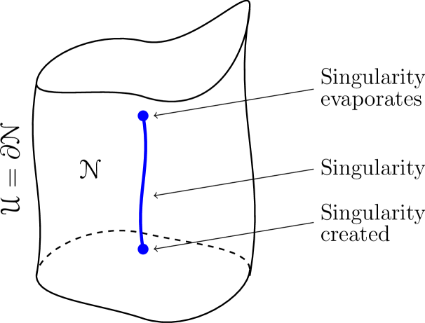
Figure 2: Here we show a region of spacetime $\mathscr{N}$ with a boundary $\mathscr{U}={\partial}\mathscr{N}$ that encloses a singularity with a finite duration. As a consequence, it is topologically non-trivial and not globally hyperbolic. This might occur, for example, due to the formation and subsequent evaporation of a black hole, which would first create and then remove a metric singularity in spacetime. If the singularity instead existed only for an instant, the blue line drawn here would reduce to a single point, and the figure would then depict the manifold $\mathscr{M}$ used in section III.

To break the topology condition (10), it is sufficient that either there is no compact spacetime region $\mathscr{N}$ such that $\mathscr{U}={\partial}\mathscr{N}$, or that there are events in $\mathscr{N}$ where $\bm{\mathsf{J}}$ is undefined. A test scenario is represented in fig. 2, where a black hole forms in an initially unremarkable spacetime, i.e. one that contains spatial hypersurfaces that are topologically trivial. On formation this introduces a singularity, but then later as the black hole evaporates, the singularity also vanishes. The evaporation step also removes the event horizon, thus exposing any effects of the singularity – e.g. in charge conservation – to the rest of the universe. In this case the singularity, which exists for a period of time before evaporating Okon-S-2018fp by means of Hawking radiation Hawking-1975cmp ; Smerlak-S-2013prd , must either be removed from spacetime, meaning that $\mathscr{N}$ is no longer topologically trivial, or alternatively that $\bm{\mathsf{J}}$ is not defined in all of $\mathscr{N}$.

Next, to break the gauge-free condition (11), we take the position that the only fundamental Maxwell’s equations are (2) and (4), that is the closure of $\bm{\mathsf{F}}$ and $\bm{\mathsf{J}}$. Since equation (3), and indeed $\bm{\mathsf{H}}$ itself, would now not be considered fundamental, $\bm{\mathsf{H}}$ may be considered as simply a potential for the current $\bm{\mathsf{J}}$. As such, it will have its own gauge freedom, as discussed in the Introduction. Writing (1) in differential form notation, for any 1-form $\psi_{\textup{g}}\in\Gamma\Lambda^{1}\mathscr{M}$, where $\psi_{\textup{g}}$ encodes $\varphi_{\textup{g}}$ and $\textbf{A}_{\textup{g}}$, we have

$$\bm{\mathsf{H}}\to\bm{\mathsf{H}}+{d}\psi_{\textup{g}}.$$ (12)

This alternative interpretation of Maxwell’s equations implies that similar to the usual 1-form potential $\bm{\mathsf{A}}$ for $\bm{\mathsf{F}}$, the excitation field $\bm{\mathsf{H}}$ is not measurable. Since $\bm{\mathsf{H}}$ is not defined absolutely, the Maxwell equation ${d}\bm{\mathsf{H}}=\bm{\mathsf{J}}$ and the constitutive relation linking $\bm{\mathsf{H}}$ to $\bm{\mathsf{F}}$ must be replaced by a constitutive relation relating the measurable quantities $\bm{\mathsf{F}}$ and $\bm{\mathsf{J}}$. This might take the form of relating $\bm{\mathsf{J}}$ to $\bm{\mathsf{F}}$ and its derivatives, for example. Thus we may interpret (3) and (5) as two aspects of a single constitutive relation for the Maxwell vacuum

$${d}{\star}\bm{\mathsf{F}}-\bm{\mathsf{J}}=0.$$ (13)

An alternative, axion-like, constitutive relation might be given by

$${d}{\star}\bm{\mathsf{F}}-\bm{\mathsf{J}}=\psi\wedge\bm{\mathsf{F}},$$ (14)

where $\psi\in\Gamma\Lambda^{1}\mathscr{M}$ is a prescribed closed 1-form. For the electromagnetic potential $\bm{\mathsf{A}}$, in (14) we can write $\bm{\mathsf{H}}={\star}\bm{\mathsf{F}}+\psi\wedge\bm{\mathsf{A}}$ but this does not define $\bm{\mathsf{H}}$ uniquely. Likewise for a (non unique) $\phi\in\Gamma\Lambda^{0}\mathscr{M}$ with ${d}\phi=\psi$ one has $\bm{\mathsf{H}}={\star}\bm{\mathsf{F}}+\phi\,\bm{\mathsf{F}}$.

When considering constitutive relations in a medium we distinguish the free current ${\bm{\mathsf{J}}_{\textup{f}}}\in\Gamma\Lambda^{3}\mathscr{M}$ from the bound current ${\bm{\mathsf{J}}_{\textup{b}}}\in\Gamma\Lambda^{3}\mathscr{M}$ representing the polarisation of the medium. The total current ${\bm{\mathsf{J}}_{\textup{t}}}\in\Gamma\Lambda^{3}\mathscr{M}$ is given by ${\bm{\mathsf{J}}_{\textup{t}}}={\bm{\mathsf{J}}_{\textup{f}}}+{\bm{\mathsf{J}}_{\textup{b}}}$. We set ${\bm{\mathsf{J}}_{\textup{f}}}=\bm{\mathsf{J}}$ in the above and describe the difference between the ${\bm{\mathsf{J}}_{\textup{f}}}$ and ${d}{\star}\bm{\mathsf{F}}$ as the bound current ${\bm{\mathsf{J}}_{\textup{b}}}$. Thus we replace (3) with

$${d}{\star}\bm{\mathsf{F}}-{\bm{\mathsf{J}}_{\textup{f}}} ={\bm{\mathsf{J}}_{\textup{b}}},$$ (15)

where ${\bm{\mathsf{J}}_{\textup{b}}}$ is related to $\bm{\mathsf{F}}$ via another constitutive relation. For example in (13), ${\bm{\mathsf{J}}_{\textup{b}}}=0$, whereas in (14) ${\bm{\mathsf{J}}_{\textup{b}}}=\psi\wedge\bm{\mathsf{F}}$. The currents ${\bm{\mathsf{J}}_{\textup{f}}}$ and ${\bm{\mathsf{J}}_{\textup{b}}}$ will be used in what follows to encode the effects of charge non-conservation.

It is worth noting that these two apparently distinct cases allowing for non-conservation of charge are related by topological considerations – the choice of spacetime with a line or point removed, the non-existence of a well-defined $\bm{\mathsf{H}}$, and the breaking of global charge conservation are all related to the deRham cohomology of the spacetime manifold.

III Singularity

In this section we construct an orientable manifold $\mathscr{M}$ on which charge is not globally conserved, even though (locally) $d\bm{\mathsf{J}}=0$ everywhere on $\mathscr{M}$. We start by assuming a flat spacetime with a Minkowski metric, except with the significant modification that a single event $\mathbf{0}$ has been removed; i.e. $\mathscr{M}={\mathbb{R}}^{4}\backslash\mathbf{0}$. This spacetime $\mathscr{M}$ is sufficient to demonstrate our mathematical and physical arguments for charge conservation failure – but without introducing any of the additional complications of (e.g.) the Schwarzschild black-hole metric. As already noted in our Introduction, the discussion here is entirely separate from and prior to any assumptions about cosmic censorship, or any imagined model of the singularity behaviour.

III.1 Charge conservation

Figure 3: A bump function ${f(\xi)}$ which we used to construct a smooth current density. The function is completely flat for $\xi>\tfrac{1}{2}$ and for $\xi$ near zero.

Let $(t,x,y,z)$ be the usual Cartesian coordinate system with $\mathbf{0}=(0,0,0,0)$ and let $(t,r,\theta,\phi)$ be the corresponding spherical coordinates. Set ${\mathbb{R}}^{+}={\left\{r\in{\mathbb{R}}|r\geq 0\right\}}$. Let us construct the smooth 3-form current density $\bm{\mathsf{J}}$ defined throughout $\mathscr{M}$ as

$$\bm{\mathsf{J}}=\begin{cases}0&\text{ for }t\leq 0,\\ \bm{\mathsf{J}}^{+}&\text{ for }t>0.\end{cases}$$ (16)

This $\bm{\mathsf{J}}^{+}$ is then defined using a function ${f}:{\mathbb{R}}^{+}\to{\mathbb{R}}^{+}$ ${{f}(\xi)}\geq 0$ for $0\leq\xi<\tfrac{1}{2}$, ${{f}(\xi)}=0$ for $\xi\geq\tfrac{1}{2}$ and all the derivatives ${{f}^{(n)}(0)}=0$ for $n\geq 1$. Such functions are usually called bump functions, an example of which is shown in fig. 3. Here $\xi$ is simply the argument of the function $f$ (and also of the function $h$ below), and it is replaced by $r/t$ when the function is used to define fields. We then have

$$\bm{\mathsf{J}}^{+} =\frac{1}{t^{3}}\,{{f}\!\left(\frac{r}{t}\right)}\,{dx}\wedge{dy}\wedge{dz}$$

$$\quad-\frac{1}{t^{4}}{{f}\!\left(\frac{r}{t}\right)}{dt}\wedge\left(x\,{dy}\wedge{dz}+y\,{dz}\wedge{dx}+z\,{dx}\wedge{dy}\right).$$ (17)

The first term on the right hand side of (17) represents the charge density, while the second term represents the current density. We note that as expressed in the Cartesian coordinates of (17), $\bm{\mathsf{J}}^{+}$ is well defined at the spatial origin for $t>0$. In spherical polar coordinates we have

$$\bm{\mathsf{J}}^{+}=\sin(\theta)~{}{{f}\!\left(\frac{r}{t}\right)}\left(\frac{r^{2}}{t^{3}}\,{dr}-\frac{r^{3}}{t^{4}}\,{dt}\right)\wedge{d\theta}\wedge{d\phi}.$$ (18)

To establish charge conservation on all of $\mathscr{M}$ with ${d}\bm{\mathsf{J}}=0$, we first note, from (18), that ${d}\bm{\mathsf{J}}^{+}=0$ for $r>0$ and $t>0$. Since $f^{(1)}(0)=0$ then, from (17), ${d}\bm{\mathsf{J}}^{+}=0$ for $t>0$ and $r=0$. Moreover, since $\bm{\mathsf{J}}=0$ for $t<0$, we have that ${d}\bm{\mathsf{J}}=0$ for $t<0$. For the hypersurface $t=0$, we note that about any point for which $r\neq 0$ there exists an open set in $\mathscr{M}$ on which $\bm{\mathsf{J}}=0$ and hence $\left.\bm{\mathsf{J}}\right|_{t=0}=0$. Thus ${d}\bm{\mathsf{J}}=0$ on all of $\mathscr{M}$.

Physically, (16) and (18) seems to represent a $\delta$-function of charge ${Q}$ appearing at the origin at $t=0$, and then spreading out spatially from $\mathbf{0}$ into $\mathscr{M}$; where

$${Q} =4\pi\int_{0}^{\infty}\xi^{2}{{f}(\xi)}{d\xi}.$$ (19)

However, the spacetime origin is not an event in $\mathscr{M}$, and the ${Q}$’s appearance at $t=0$ does not induce ${d}J\neq 0$ at some event in $\mathscr{M}$. We see that the total charge is zero for the constant-time hypersurfaces with $t<0$, but for the constant-time hypersurfaces with $t>0$ the charge is ${Q}$.

Similarly, over a region such as that shown in figs. 1 and 2 we have that $\int_{\mathscr{U}}\bm{\mathsf{J}}\neq 0$. Charge is therefore not conserved in $\mathscr{M}$, despite the fact that ${d}\bm{\mathsf{J}}=0$ everywhere in $\mathscr{M}$.

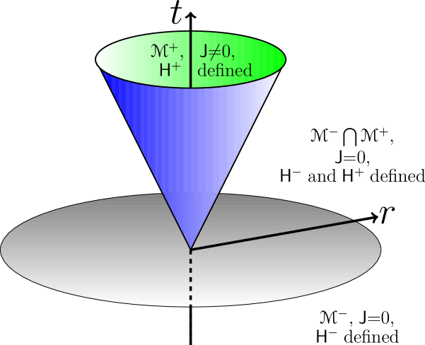
Figure 4: A spacetime $\mathscr{M}$ in which charge is not conserved. The forward cone, lying within the lightcone of the excised event at $\mathbf{0}$ has non-zero charge, whereas the remainder of the spacetime is uncharged. We show the regions $\mathscr{M}^{+}$ and $\mathscr{M}^{-}$ where the excitation 2-forms $\bm{\mathsf{H}}^{+}$ and $\bm{\mathsf{H}}^{-}$ are defined.

Now since $\mathscr{M}$ is topologically non-trivial, it is impossible to find a single $\bm{\mathsf{H}}$ such that ${d}\bm{\mathsf{H}}=0$. This must be the case since if it were not, then we could apply (11) to establish ${Q}=0$. Nevertheless we can find two fields $\bm{\mathsf{H}}^{+}$ and $\bm{\mathsf{H}}^{-}$ with intersecting domains $\mathscr{M}^{+}$ and $\mathscr{M}^{-}$ such that on the intersection, $\bm{\mathsf{H}}^{+}=\bm{\mathsf{H}}^{-}+{d}\psi$, i.e they differ by just a gauge, as per (12). Let

$$\mathscr{M}^{+}=\mathscr{M}\backslash{\left\{t<0\right\}}~{}~{}\textrm{and}~{}~{}\mathscr{M}^{-}=\mathscr{M}\backslash{\left\{t>0~{}\textrm{and}~{}r<\tfrac{1}{2}t\right\}},$$ (20)

and with $\bm{\mathsf{H}}^{+}\in\Gamma\Lambda^{2}\mathscr{M}^{+}$ and $\bm{\mathsf{H}}^{-}\in\Gamma\Lambda^{2}\mathscr{M}^{-}$, let

$$\bm{\mathsf{H}}^{+} ={{h}\left(\frac{r}{t}\right)}\left(x\,{dy}\wedge{dz}+y\,{dz}\wedge{dx}+z\,{dx}\wedge{dy}\right)$$

$$={{h}\left(\frac{r}{t}\right)}\left(r^{3}\sin\theta\,{d\theta}\wedge{d\phi}\right),$$

$$\bm{\mathsf{H}}^{-} =0,$$

as depicted in fig. 4. Here

$${{h}(\xi)} =\frac{1}{\xi^{3}}\int_{0}^{\xi}{{f}({\hat{\xi}})}\,\hat{\xi}^{2}d\hat{\xi}.$$ (21)

Since ${{h}(\xi)}$ is smooth about $\xi=0$ and

$${{h}(\xi)}=\frac{{Q}}{4\pi\xi^{3}}\quad\textup{for}\quad\xi>\tfrac{1}{2},$$ (22)

then on the intersection $\mathscr{M}^{+}\bigcap\mathscr{M}^{-}$$={\left\{\left.\left(t,r,\theta,\phi\right)\,\right|\,r>t>0\right\}}$ we have

$$\bm{\mathsf{H}}^{+}=\frac{{Q}}{4\pi}\sin(\theta){d\theta}\wedge{d\phi}\qquad\textup{and}\qquad\bm{\mathsf{H}}^{-}=0.$$ (23)

Therefore $\bm{\mathsf{H}}^{+}=\bm{\mathsf{H}}^{-}-({Q}/4\pi){d\left(\cos(\theta)\,{d\phi}\right)}$ for the region ${\left\{\left.(t,r,\theta,\phi)\,\right|\,r>t>0,\theta\neq 0,\pi\right\}}$. Choosing other patches of the $(\theta,\phi)$ sphere we can find other gauge fields $\psi$ such that $\bm{\mathsf{H}}^{+}=\bm{\mathsf{H}}^{-}+{d}\psi$. In this example, there is no global $\bm{\mathsf{H}}$-field, and both $\bm{\mathsf{H}}^{+}$ and $\bm{\mathsf{H}}^{-}$ fail in distinct regions of $\mathscr{M}$. This strongly suggests that $\bm{\mathsf{H}}$ need not have absolute physical significance, unlike $\bm{\mathsf{F}}$.

The new gauge freedom for $\bm{\mathsf{H}}$ suggests the possibility of further generalisations to the vacuum constitutive relations. These could now go beyond rather prescriptive vaccum models such as e.g. the Euler-Heisenberg or Bopp-Podolsky ones in (6) and (7), whose Lagrangian formulations insist on a unique $\bm{\mathsf{H}}$.

IV Polarisation of the vacuum

We now stay with the same scenario as in the previous section, but instead apply the bound current version of Maxwell theory as given by (15), interpreting ${\bm{\mathsf{J}}_{\textup{b}}}$ as representing the polarisation of the vacuum. It is known from quantum field theory that vacuum polarization occurs naturally for intense fields, with the first order correction to the excitation 2-form given by (6). Indeed, the strong magnetic fields associated with magnetars are known to induce non-trivial dielectric properties on vacuum Lai-H-2003aj . An alternative model for the polarization of the vacuum is given by the Bopp-Podolski theory of electromagnetism, as outlined in (7). However in these cases the bound currents ${\bm{\mathsf{J}}_{\textup{b}}}^{\!\!\!\!\textup{EH}}=d\bm{\mathsf{H}}_{\textup{EH}}-{d}{\star}\bm{\mathsf{F}}$ and ${\bm{\mathsf{J}}_{\textup{b}}}^{\!\!\!\!\textup{BP}}=d\bm{\mathsf{H}}_{\textup{BP}}-{d}{\star}\bm{\mathsf{F}}$ correspond to a well defined excitation 2-form $\bm{\mathsf{H}}$ and therefore must conserve charge, regardless of topology. Nevertheless we are still free to consider more general versions of ${\bm{\mathsf{J}}_{\textup{b}}}$ which are not exact and contain more than just those corrections.

Since ${\star}\bm{\mathsf{F}}$ is well defined, and ${d}{\star}\bm{\mathsf{F}}={\bm{\mathsf{J}}_{\textup{f}}}+{\bm{\mathsf{J}}_{\textup{b}}}$, one can use the argument (11), replacing $\bm{\mathsf{H}}$ with ${\star}\bm{\mathsf{F}}$, to conclude that ${\bm{\mathsf{J}}_{\textup{f}}}+{\bm{\mathsf{J}}_{\textup{b}}}$ is globally conserved. We now examine whether it is necessary for ${\bm{\mathsf{J}}_{\textup{f}}}$ and ${\bm{\mathsf{J}}_{\textup{b}}}$ to be globally conserved independently. If $\bm{\mathsf{H}}$ is well defined then from (3) (which now becomes $d\bm{\mathsf{H}}={\bm{\mathsf{J}}_{\textup{f}}}$) ${d}{\bm{\mathsf{J}}_{\textup{f}}}=0$ and hence ${d}{\bm{\mathsf{J}}_{\textup{b}}}=0$. Under these circumstances, we find that ${\bm{\mathsf{J}}_{\textup{f}}}$ by itself is globally conserved, and likewise for ${\bm{\mathsf{J}}_{\textup{b}}}$ by itself.

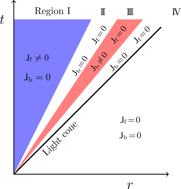
Figure 5: Domains in a spacetime $\mathscr{M}$ where ${\bm{\mathsf{J}}_{\textup{f}}}$ (blue) and ${\bm{\mathsf{J}}_{\textup{b}}}$ (red) may be non-zero; note in particular that the supports of ${\bm{\mathsf{J}}_{\textup{f}}}$ and ${\bm{\mathsf{J}}_{\textup{b}}}$ do not intersect. For completeness, we show several different regions where the various possible combinations of zero and non-zero ${\bm{\mathsf{J}}_{\textup{f}}}$ and ${\bm{\mathsf{J}}_{\textup{b}}}$ hold, although alternative (and simpler) scenarios are possible. Note that Region I matches the cone shown on fig. 4, and Region I​V encompasses both a section above the light line, as well as below.

In the following, we demand only that ${\bm{\mathsf{J}}_{\textup{f}}}$ and hence ${\bm{\mathsf{J}}_{\textup{b}}}$ are closed: $d{\bm{\mathsf{J}}_{\textup{f}}}=d{\bm{\mathsf{J}}_{\textup{b}}}=0$, and do not insist that they are globally conserved independently. This requires us to abandon the concept of a global macroscopic well-defined $\bm{\mathsf{H}}$, and to express the constitutive relations for our spacetime using the microscopic bound current, ${\bm{\mathsf{J}}_{\textup{b}}}$. Unlike $\bm{\mathsf{F}}$, the excitation $\bm{\mathsf{H}}$ cannot be measured directly using either the Lorentz force equation or the Aharonov-Bohm effect.

To demonstrate our replacement of $\bm{\mathsf{H}}$, we now show that we can replace it with a bound current. We start by choosing an appropriate $\bm{\mathsf{F}}$, setting

$$\bm{\mathsf{F}} =h\!\left(\frac{r}{t}\right)\chi\!\left(\frac{r}{t}\right){\textup{hv}}(t)\,r\,{dt}\wedge{dr}={{R}\left(\frac{r}{t}\right)}\,r\,{dt}\wedge{dr},$$ (24)

where

(i)

$h(\xi)$ is defined from (21), i.e. $h(\xi)=\frac{1}{\xi^{3}}\int_{0}^{\xi}f({\hat{\xi}}){\hat{\xi}}^{2}d{\hat{\xi}}$.

(ii)

$f:{\mathbb{R}}^{+}\rightarrow{\mathbb{R}}^{+}$ is again a bump function satisfying $f(\xi)\geq 0$ for $0<\xi<1/2$, $f(\xi)=0$ for $\xi\geq 1/2$, and $f^{(n)}=0$ for $n\geq 1$.

(iii)

${\textup{hv}}:{\mathbb{R}}\to{\mathbb{R}}$ is the Heaviside step function.

(iv)

${\chi}:{\mathbb{R}}^{+}\to{\mathbb{R}}$ is a bump function with ${{\chi}(\xi)}=1$ for $0\leq\chi<\tfrac{2}{3}$ and ${{\chi}(\xi)}=0$ for $\xi>\tfrac{5}{6}$.

Clearly ${d}\bm{\mathsf{F}}=0$. The scalar factor ${{R}(\xi)}$ on the right hand side of (24) has the following properties

$${{R}\left(\frac{r}{t}\right)} =\! \left\{\begin{array}[]{ll@{\quad}l}\rule[-6.0pt]{0.0pt}{12.0pt}~{}~{}0&\text{ for }t<0,&\\ \rule[-6.0pt]{0.0pt}{12.0pt}~{}~{}{{h}\!\left(\frac{r}{t}\right)}&\text{ for }0\leq r<\tfrac{1}{2}t,&\textrm{Region~{}{{{I}}}}\\ \rule[-6.0pt]{0.0pt}{12.0pt}\frac{Q}{4\pi r^{3}}&\text{ for }0<\tfrac{1}{2}t<r<\tfrac{2}{3}t,\!&\textrm{Region~{}{{{I\!I}}}}\\ \rule[-6.0pt]{0.0pt}{12.0pt}{{\chi}\!\left(\frac{r}{t}\right)}\frac{Q}{4\pi r^{3}}\!&\text{ for }0<\tfrac{2}{3}t<r<\tfrac{5}{6}t,\!&\textrm{Region~{}{{{I\!I\!I}}}}\\ \rule[-6.0pt]{0.0pt}{12.0pt}~{}~{}0&\text{ for }0<\tfrac{5}{6}t<r,&\textrm{Region~{}{{{I\!V}}}}\end{array}\right.$$ (30)

(31)

where $Q$ is given by (19), and the regions I to I​V are shown in fig. 5. These regions contain a selection of the possible combinations of ${\bm{\mathsf{J}}_{\textup{f}}}$ and ${\bm{\mathsf{J}}_{\textup{b}}}$. We can then set the constitutive relation to be that of (15), with ${\bm{\mathsf{J}}_{\textup{f}}},{\bm{\mathsf{J}}_{\textup{b}}}\in\Gamma\Lambda^{3}\mathscr{M}$ being independently conserved, but only in a local sense, not globally. For our example, they are respectively given by

$${\bm{\mathsf{J}}_{\textup{f}}}=\left\{\begin{array}[]{ll@{\quad}l}\displaystyle d{\star}\bm{\mathsf{F}}&\text{ for }0<r<\tfrac{1}{2}t,\hfill\qquad\qquad\qquad\text{in Region~{}{{{I}}}}\\ \rule[-6.0pt]{0.0pt}{12.0pt}0&\text{ for }t<0\text{ and }\tfrac{1}{2}t<r<t,\\ &\hfill\text{in Regions~{}{{{I\!I}}}, {{{I\!I\!I}}} and {{{I\!V}}}}\end{array}\right.$$ (32)

and  

$${\bm{\mathsf{J}}_{\textup{b}}}=\left\{\begin{array}[]{ll@{\quad}l}0&\text{ for }t<0\text{ and }0<r<\tfrac{2}{3}t\text{ and }0<\tfrac{5}{6}t<r,{}\\ &\hfill\text{in Regions~{}{{{I}}}, {{{I\!I}}} and {{{I\!V}}}}\\ \rule[-6.0pt]{0.0pt}{12.0pt}\displaystyle d{\star}\bm{\mathsf{F}}\!&\text{ for }0<\tfrac{2}{3}t<r<\tfrac{5}{6}t,\hfill\text{in Region~{}{{{I\!I\!I}}}}\end{array}\right.$$ (33)

or explicitly as

$${\bm{\mathsf{J}}_{\textup{f}}}=\left\{\begin{array}[]{ll@{\quad}l}\displaystyle{{h}^{\prime}\left(\frac{r}{t}\right)}\left[\left(\frac{r^{3}}{t}+3r^{2}\right)\,{dr}-\frac{r^{4}}{t^{2}}{dt}\right]\wedge\sin(\theta){d\theta}\wedge{d\phi}\\ \hfill\text{ for }0<r<\tfrac{1}{2}t,\qquad\text{in Region~{}{{{I}}}}\\ \rule[-6.0pt]{0.0pt}{12.0pt}\displaystyle 0\hfill\text{ for }\tfrac{1}{2}t<r<t,\qquad\text{in Regions~{}{{{I\!I}}}, {{{I\!I\!I}}} and {{{I\!V}}}}\end{array}\right.$$ (34)

and

$${\bm{\mathsf{J}}_{\textup{b}}}=\left\{\begin{array}[]{ll}0\hfill\qquad\text{ for }t<0\text{ and }0<r<\tfrac{2}{3}t\text{ and }0<\tfrac{5}{6}t<r,\\ \hfill\qquad\text{in Regions~{}{{{I}}}, {{{I\!I}}} and {{{I\!V}}}}\\ \rule[-6.0pt]{0.0pt}{12.0pt}\displaystyle\frac{{Q}}{4\pi}{{\chi}^{\prime}\left(\frac{r}{t}\right)}\left[\frac{1}{t}\,{dr}-\frac{r}{t^{2}}{dt}\right]\wedge\sin(\theta){d\theta}\wedge{d\phi}\\ \hfill\qquad\text{ for }0<\tfrac{2}{3}t<r<\tfrac{5}{6}t,\qquad\text{in Region~{}{{{I\!I\!I}}}}.\end{array}\right.$$ (35)

The occurrence of a bound charge of single sign over an extended region of space may seem rather unusual. However, this can be realised in a dielectric with a continuously varying permittivity. For example, a constant bound charge density $\lambda$ can be obtained with the dielectric varying as

$${{\epsilon}(z)} =\epsilon_{0}+\epsilon_{0}\frac{P_{0}-\lambda\,z}{\epsilon_{0}\,V_{0}+\lambda\,z},$$ (36)

which gives

$${{E}(z)}=\frac{\lambda\,z}{\epsilon_{0}}+V_{0}\quad\textup{and}\quad{{P}(z)}=P_{0}-\lambda\,z,$$ (37)

for constants $V_{0}$ and $P_{0}$.

In writing (24) the distinction between free and bound current densities, as arise in the subsequent calculations, is introduced artificially. So whilst our introduced example is certainly artificial, it can be taken to be representative and illustrative of a scenario in which the 2-form field $\bm{\mathsf{H}}$ is no longer globally defined; but that the sum of free and bound charge densities in vacuum is globally conserved, while the two types of charge are not collectively globally conserved, and exist independently in disjoint regions of space. This echoes the previous section, but here we use the non-exactness of $\bm{\mathsf{J}}$ rather than the gauge freedom for $\bm{\mathsf{H}}$; thus suggesting generalisations to the charge and polarization properties of the vacuum constitutive relations.

V Wormhole

A wormhole Morris-T-1988ajp is another example of a non-trivial spacetime, although in this case it is the first deRham cohomology which does not vanish, $\bm{\mathsf{H}}^{1}_{\textup{dR}}={\mathbb{R}}$. In this scenario we do not break conservation of global charge, but instead address the issue of whether a wormhole necessarily gains the charge of any matter passing through it. One simple way of describing this standard viewpoint is to note that the usual process of drawing field lines for a charge, as it moves, forbids them from swapping their end-points from one place to another. This means that a positive charge passing through a wormhole “drags” its field lines behind it like a tail, and the resulting collection of field lines re-entering the wormhole looks like a negative charge, and then as they exit the other side they look like a positive charge; as depicted in fig. 6.

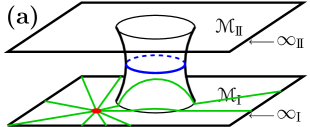
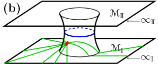
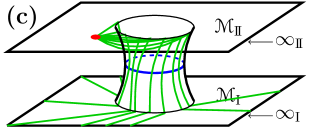
Figure 6: A depiction of the standard interpretation of field line behaviour as a charge $q$ moves from the lower universe $\mathscr{M}_{\textup{I}}$ (a), through the wormhole (b), and into the upper universe $\mathscr{M}_{\textup{I\!I}}$ (c) – all the field lines (green) from the point charge (red dot) must remain attached to $\infty_{\textup{I}}$. Note that despite the similarity in relative charge-wormhole positions between the starting point in (a) and the end point in (c), the field line configuration is very different. Consequently, as the charge moves ever further from the wormhole mouth in $\mathscr{M}_{\textup{I\!I}}$, the effective charges in the biverse would number three and not one: $\mathscr{M}_{\textup{I}}$ has a wormhole mouth with field lines exiting it on the way to infinity, and which integrate to $+{q}$, whilst $\mathscr{M}_{\textup{I\!I}}$ has an overall dipole-like field between an effective charge $-{q}$ on the wormhole mouth and the free charge $+{q}$.

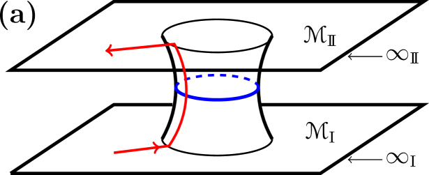
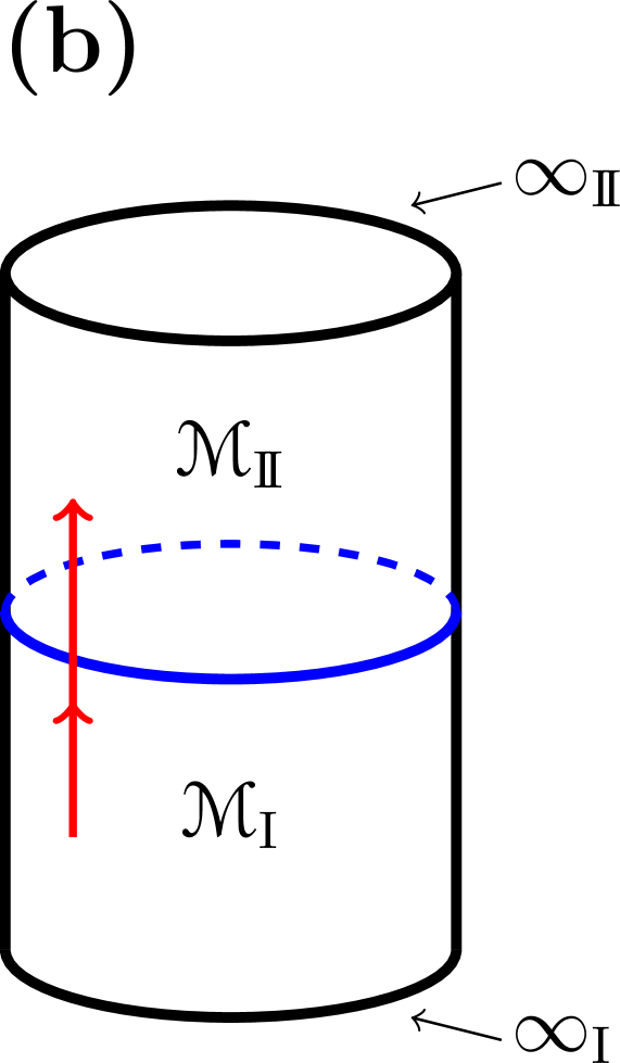
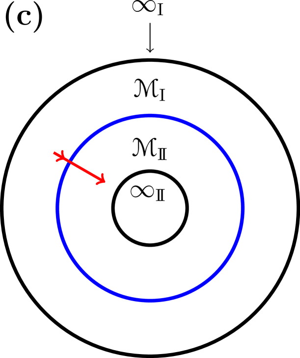
Figure 7: Deforming a “biverse”, i.e. two otherwise distinct universes interconnected by a wormhole, into an annulus. When deforming from (a) into (b), the wormhole’s throat (blue line) is unchanged, whilst the top ($\mathscr{M}_{\textup{I\!I}}$) and bottom ($\mathscr{M}_{\textup{I}}$) universes are deformed into cylinders. The final stage from (b) to (c) requires opening out the cylinders into two nested annuli, which form a single annulus with the throat demarking the join. The red line in each diagram represents the path for a point charge leaving $\mathscr{M}_{\textup{I}}$ and entering $\mathscr{M}_{\textup{I\!I}}$.

The proof of conservation of charge is similar to the arguments of (10) and (11) but in this case the two arguments have different interpretations. First we note from fig. 7 that spatially the wormhole is topologically equivalent to a 3-dimensional annulus, i.e. a 3-ball with an inner 3-ball removed. The inner and outer 2-spheres $\infty_{\textup{I}}$ and $\infty_{\textup{I\!I}}$ represent spacelike infinity in the two universes $\mathscr{M}_{\textup{I}}$ and $\mathscr{M}_{\textup{I\!I}}$. Between the two 2-spheres there is a concentric sphere which is the throat. Although geometrically the throat is the minimum size sphere which connects the two universes, topologically there is nothing special about the throat, and here we take it as a convenient place to talk about where one passes from one universe to the other. Further, since each universe ($\mathscr{M}_{\textup{I}}$ or $\mathscr{M}_{\textup{I\!I}}$) has its own infinity ($\infty_{\textup{I}}$ or $\infty_{\textup{I\!I}}$), there are two ways to be arbitrarily far from the wormhole, and thus there are two possible destinations for the field lines of a charge.

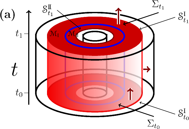
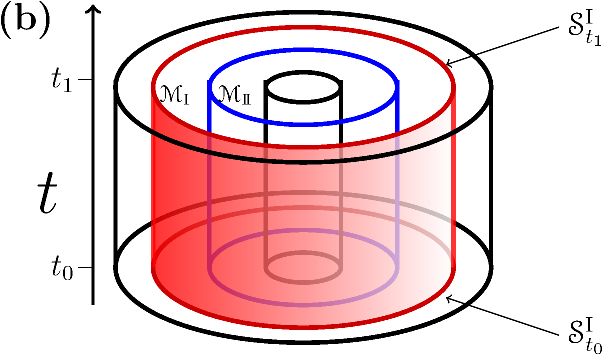
Figure 8: Integration submanifolds for our wormhole example of fig. 7. The upper diagram (a) is for integrating $\bm{\mathsf{J}}$, whereas the lower diagram (b) is for integrating $\bm{\mathsf{H}}$. The orientation is shown in dark red.

Consider the 3-dimensional region ${\Sigma}$ bounded by the spheres $\mathscr{S}^{\textup{I}}$ and $\mathscr{S}^{\textup{I\!I}}$. Then, as illustrated in fig. 8(a), $[t_{0},t_{1}]\times{\Sigma}$ is a 4-dimensional region bounded by ${\Sigma}_{t_{0}}$, ${\Sigma}_{t_{1}}$, $[t_{0},t_{1}]\times\mathscr{S}^{\textup{I\!I}}$ and $[t_{0},t_{1}]\times\mathscr{S}^{\textup{I}}$. Then

$$0 =~{}~{}\int_{[t_{0},t_{1}]\times{\Sigma}}{d}\,\bm{\mathsf{J}}=~{}~{}\int_{{\partial}\left(\rule{0.0pt}{4.89998pt}[t_{0},t_{1}]\times{\Sigma}\right)}\bm{\mathsf{J}}$$

$$=\int_{{\Sigma}_{t_{1}}}\bm{\mathsf{J}}-\int_{{\Sigma}_{t_{0}}}\bm{\mathsf{J}}+\int_{[t_{0},t_{1}]\times\mathscr{S}^{\textup{I\!I}}}\bm{\mathsf{J}}+\int_{[t_{0},t_{1}]\times\mathscr{S}^{\textup{I}}}\bm{\mathsf{J}}.$$ (38)

This states that the total charge in ${\Sigma}$ at time $t_{1}$ equals the charge in ${\Sigma}$ at time $t_{0}$ plus any charge that enters (or leaves) via $\mathscr{S}^{\textup{I\!I}}$ and $\mathscr{S}^{\textup{I}}$. We cannot let $\mathscr{S}^{\textup{I}}$ go to infinity as then it would disappear from the right hand side of (38) and Stokes’ theorem will no longer apply.

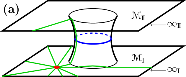
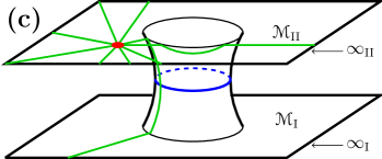
Figure 9: Depiction of the alternative field line behavior when allowing for the topology and the new freedom for $\bm{\mathsf{H}}$. Field lines (green) in the biverse all start a the point charge (red dot), but now have a choice of infinity at which to terminate. Initially, when the charge is (a) well within universe I, relatively few field lines reach through the wormhole into universe I​I and hence off to $\infty_{\textup{I\!I}}$, but as the point charge moves into to the throat (b) more of the field lines will reach $\infty_{\textup{I\!I}}$. In (c) we see that after the charge has moved fully into universe II, in a position mirroring that in (a), the arrangement of field lines is also mirrored, in distinct contrast with the standard treatment of fig. 6.

Another issue arises when considering the second proof of charge conservation (cf. (11)). If $\bm{\mathsf{H}}$ is a well-defined $2$-form field we may integrate it over the 3-dimensional timelike hypersurface $[t_{0},t_{1}]\times\mathscr{S}^{\textup{I}}$, fig. 8(b). Setting ${Q}^{\textup{I}}_{t}=\int_{\mathscr{S}^{\textup{I}}_{t}}\bm{\mathsf{H}}$ as the charge inside $\mathscr{S}^{\textup{I}}$ at time $t$, we have

$${Q}^{\textup{I}}_{t_{1}}-{Q}^{\textup{I}}_{t_{0}} =~{}~{}\int_{\mathscr{S}^{\textup{I}}_{t_{1}}}\bm{\mathsf{H}}-\int_{\mathscr{S}^{\textup{I}}_{t_{0}}}\bm{\mathsf{H}}=~{}~{}\int_{{\partial}\left([t_{0},t_{1}]\times\mathscr{S}^{\textup{I}}\rule{0.0pt}{4.89998pt}\right)}\bm{\mathsf{H}}$$

$$=~{}~{}\int_{[t_{0},t_{1}]\times\mathscr{S}^{\textup{I}}}{d}\bm{\mathsf{H}}=~{}~{}\int_{[t_{0},t_{1}]\times\mathscr{S}^{\textup{I}}}\bm{\mathsf{J}}.$$ (39)

Thus if $\bm{\mathsf{H}}$ is well-defined, and no current passes through $\mathscr{S}^{\textup{I}}$, then ${Q}_{t}^{\textup{I}}$ is a conserved quantity. When a charge $q$ located within the sphere $\mathscr{S}_{\textup{I}}$ passes though the throat of the wormhole to $\mathscr{M}_{\textup{I\!I}}$, an observer in $\mathscr{M}_{\textup{I}}$ who has merely integrated $\bm{\mathsf{H}}$ over $\mathscr{S}^{\textup{I}}$ to establish the conserved quantity ${Q}_{t}^{\textup{I}}$, no longer sees $q$ in their part of the universe. They rather say that after the charge has passed though the throat, the wormhole has gained charge $q$ Visser-LW ; Susskind-2005arXiv ; Wheeler-1957ap .

There may still be aspects of this standard “charged wormhole” view that worry some. Of course, if a charge enters a box, the charge will still be in the box whenever we subsequently look inside, and we can reasonably say that the box has acquired that charge. However, in the current case, after passing to universe $\mathscr{M}_{\textup{I\!I}}$, the charge $q$ might subsequently move arbitrarily far from the throat. At such a distance, some might consider it unreasonable to have the steady-state field of the charge still influenced by some prehistoric transit from $\mathscr{M}_{\textup{I}}$. Nevertheless, the standard viewpoint insists that an observer in $\mathscr{M}_{\textup{I}}$ still sees that the wormhole has acquired, and retained, charge $q$.

However, since our biverse scenario has a non-trivial topology, we can again consider $\bm{\mathsf{H}}$ to be undefined in an absolute sense. Having decided that $\bm{\mathsf{H}}$ is not defined, one is free to consider how to replace it. We consider here a simple extension to Maxwell’s equations in which the charge the wormhole gains depends on the distance from the charge to the throat, and is no longer affected by whether or not the charge made a one-way transit through that throat in the past.

Consider a single point charge $q$, and define ${{Q}^{\textup{I}}({r_{p}})}$ as a function of the radial position, ${r_{p}}$ of the charge. Thus we can set

$${{Q}^{\textup{I}}({r_{p}})} ={q}\,{{\zeta}({r_{p}})}$$ (40)

$$\qquad\textup{where}\qquad{{\zeta}({r_{p}})} =\frac{1}{2}+\frac{\delta{r_{p}}}{2(r_{\textup{th}}^{2}+{\delta{r_{p}}}^{2})^{1/2}},$$ (41)

and where $r_{\textup{th}}$ is the radius of the throat and ${\delta{r_{p}}}$ is the distance to the throat with ${\delta{r_{p}}}>0$ and ${\delta{r_{p}}}<0$ if the charge is in $\mathscr{M}_{\textup{I}}$ and $\mathscr{M}_{\textup{I\!I}}$ respectively. Although this function is arbitrary it does have the useful feature that ${{Q}^{\textup{I}}(r_{p})}\to q$ if ${r_{p}}\to\infty_{\textup{I}}$ and the ${{Q}^{\textup{I}}(r_{p})}\to 0$ if ${r_{p}}\to\infty_{\textup{I\!I}}$, and is inline with physical intuition.

We note below that the field $\bm{\mathsf{H}}$ is still well-defined as long as the charge is moving slowly, $d{r_{p}}/dt\approx 0$. Let $\bm{\mathsf{F}}^{\textup{I}}_{r_{p}}\in\Gamma\Lambda^{2}\mathscr{M}$ and $\bm{\mathsf{F}}^{\textup{I\!I}}_{r_{p}}\in\Gamma\Lambda^{2}\mathscr{M}$ be the static electromagnetic field for a point charge at ${r_{p}}$, so that

$${d}\bm{\mathsf{F}}^{\textup{I}}_{r_{p}}=0\,,\qquad{d}\bm{\mathsf{F}}^{\textup{I\!I}}_{r_{p}}=0\,,\qquad{d}{\star}\bm{\mathsf{F}}^{\textup{I}}_{r_{p}}=\bm{\mathsf{J}}_{r_{p}},$$

$$\qquad\qquad\textup{and}\qquad{d}{\star}\bm{\mathsf{F}}^{\textup{I\!I}}_{r_{p}}=\bm{\mathsf{J}}_{r_{p}},$$ (42)

where $\bm{\mathsf{J}}_{r_{p}}$ is the distributional source corresponding to a point charge at $r={r_{p}}$, $\theta=0$ and $\phi=0$

$$\bm{\mathsf{J}}_{r_{p}}=\,q{{\delta}(r-r_{p})}\,{{\delta}(\theta)}\,{{\delta}(\phi)}\,r^{2}\sin\theta~{}{dr}\wedge{d\theta}\wedge{d\phi},$$ (43)

subject to the boundary conditions

$$\lim_{r\to\infty_{\textup{I}}}\bm{\mathsf{F}}^{\textup{I}}=0\,, \qquad\lim_{r\to\infty_{\textup{I\!I}}}r^{2}\bm{\mathsf{F}}^{\textup{I}}=0,$$

$$\lim_{r\to\infty_{\textup{I}}}r^{2}\bm{\mathsf{F}}^{\textup{I\!I}}=0\,, \qquad\lim_{r\to\infty_{\textup{I\!I}}}\bm{\mathsf{F}}^{\textup{I\!I}}=0.$$ (44)

That is to say the field lines for $\bm{\mathsf{F}}^{\textup{I}}$ due to the point charge all terminate at $\infty_{\textup{I}}$, whereas those for $\bm{\mathsf{F}}^{\textup{I\!I}}$ terminate at $\infty_{\textup{I\!I}}$. Let

$$\bm{\mathsf{H}}_{r_{p}}={{\zeta}({r_{p}})}\,{\star}\bm{\mathsf{F}}^{\textup{I\!I}}_{r_{p}}+\left[1-{{\zeta}({r_{p}})}\right]\,{\star}\bm{\mathsf{F}}^{\textup{I}}_{r_{p}}$$ (45)

which has the property that, as long as the point charge is inside $\mathscr{S}^{\textup{I}}$, which includes all of $\mathscr{M}_{\textup{I\!I}}$, then

$${Q}^{\textup{I}}_{r_{p}}=\int_{\mathscr{S}^{\textup{I}}}\bm{\mathsf{H}}_{r_{p}}.$$ (46)

Thus as the point charge moves closer to the throat more of the field lines reach $\infty_{\textup{I\!I}}$, fig. 9. However we only approximately solve Maxwell’s equations since

$${d}\,\bm{\mathsf{H}}_{r_{p}} =\bm{\mathsf{J}}_{r_{p}}+{{\zeta}^{\prime}(r_{p})}\,\dfrac{r_{p}}{t}\,{dt}\wedge{\star}\left(\bm{\mathsf{F}}^{\textup{I}}_{r_{p}}-F^{\textup{I\!I}}_{r_{p}}\right)$$

$$\qquad+{{\zeta}(r_{p})}\,\dfrac{r_{p}}{t}\,{dt}\wedge{\star}\left(\dfrac{\bm{\mathsf{F}}^{\textup{I}}_{r_{p}}}{r_{p}}-\dfrac{\bm{\mathsf{F}}^{\textup{I\!I}}_{r_{p}}}{r_{p}}\right).$$ (47)

However, we again emphasise that we cannot define a $\bm{\mathsf{H}}_{r_{p}}$ which solves both Maxwell’s equations and eqn. (46).

Another attractive feature of our proposed modification occurs in relation to a wormhole connecting two distinct regions ($\mathscr{A}$ and $\mathscr{B}$, say) in the same universe. In this topology, a charge ${q}$ can circulate multiple ($n$, say) times by entering at $\mathscr{A}$ and exiting at $\mathscr{B}$. Standard Maxwell theory then predicts that $\mathscr{A}$ has a charge of $n{q}$, and $\mathscr{B}$ a charge of $-n{q}$, which can become arbitrarily large. The modification to Maxwell’s theory of (44) avoids this problem, as integrating around $\mathscr{A}$ will yield a charge that does not exceed $q$.

VI Discussion

There are mechanisms for charge conservation that exist independently of the topology or gauge-free conditions that we have discussed above. One of the most notable is a consequence of Noether’s theorem for a $U(1)$ gauge invariant Lagrangian, which enforces local charge conservation ${d}\bm{\mathsf{J}}=0$. For example, if $\Lambda[\bm{\mathsf{A}},\alpha]\in\Gamma\Lambda^{4}\mathscr{M}$ is invariant under substitutions $\alpha\rightarrow e^{\imath\phi}\alpha$ and $\bm{\mathsf{A}}\rightarrow\bm{\mathsf{A}}+\imath{d}\phi$, then the 3-form $\partial\Lambda/\partial\bm{\mathsf{A}}$ is locally conserved, i.e. ${d}(\partial\Lambda/\partial\bm{\mathsf{A}})=0$. Since the variations are purely local, this makes no statement about the global conservation of charge in non trivial spacetimes. It should also be noted that most Lagrangian formulations of electromagnetism implicitly assume a model for $\bm{\mathsf{H}}$. For example the Maxwell vacuum where $\Lambda$ contains the term $\Lambda^{\textup{EM}}=\frac{1}{2}{d}\bm{\mathsf{A}}\wedge\star{d}\bm{\mathsf{A}}$, or a model of a simple non-dispersive “antediluvian” medium where $\Lambda^{\textup{EM}}=\frac{1}{2}{d}\bm{\mathsf{A}}\wedge\star\bm{\mathsf{Z}}({d}\bm{\mathsf{A}})$ and $\bm{\mathsf{Z}}$ is a constitutive tensor Gratus-T-2011jmp . It would also be interesting to attempt to construct Lagrangians which do not imply a well defined excitation 2-form.

We might also broaden our examination of conservation laws beyond just charge to those of energy and momentum, by looking at the divergence-free nature of the stress-energy tensor T. In our discussion of section III, the total energy of the current and electromagnetic field must be zero before the singularity, i.e. on a hypersuface in $\mathscr{M}^{-}$. Likewise, although we did not define the energy, the existence of fields after the singularity, implies that the total energy would be non zero. However, just as in the case of charge conservation, this lack of global energy conservation is not inconsistent with the local energy conservation law ${d}({\bm{\mathsf{\tau}}_{K}})=0$, obtained from the energy 3-form $\bm{\mathsf{\tau}}_{K}=\star\textbf{T}({K},-))$, where $K$ is a timelike Killing field. Of course, in the general relativistic case of an evaporating black hole there are challenges about defining the total energy, but one should not be surprised if an appropriate measure of total energy were also not conserved.

For momentum, if $\mathscr{M}$ possesses a spacelike Killing vector ${K}$, then ${K}$ is locally conserved, i.e. ${d}({\bm{\mathsf{\tau}}_{K}})=0$, but again this has said nothing about the global conservation of momentum. We see from (18) that the construction of $\bm{\mathsf{J}}$ that it is spherically symmetric and hence will not change the total momentum. However, this was a choice and non-spherically symmetric currents can easily be obtained by introducing a Lorentz boost. Of course, when considering the total momentum, i.e. that of the electromagnetic field plus that of the response of the medium, one encounters the thorny issue of the Abraham-Minkowski controversy Dereli-GT-2007pla ; Dereli-GT-2007jpa and choice of Poynting vector Kinsler-FM-2009ejp . From the perspective here, the question of which momentum is most appropriate would be further complicated by the non existence of the excitation 2-form.

As a final remark, our results presented here raise the possibility of developing a way to prescribe dynamic equations for the electromagnetic field $\bm{\mathsf{F}}$ without introducing or referring to an excitation field $\bm{\mathsf{H}}$ at all. One possibility is to combine Maxwell’s equation (3) directly with the constitutive relations, thus eliminating the need for $\bm{\mathsf{H}}$ Gratus-MK-AREA51 .

VII Conclusion

In this paper we have clarified physical issues regarding electromagnetism on spacetimes with a non-trivial topology – either missing points, as can be introduced by the singularity at the heart of a black hole, or the presence of wormhole-like bridges between universes, or between two locations in the same universe.

We have unambiguously shown that such cases have significant implications for charge conservation – i.e. that it need not be conserved; and the role of (or need for) the electromagnetic excitation field $\bm{\mathsf{H}}$ (i.e. the Maxwell D, H vector fields) – i.e. that it is not always globally unique, and thus has a subordinate or even optional status as compared to the more fundamental $\bm{\mathsf{F}}$ comprising the Maxwell E, B vector fields. All of these considerations are purely electromagnetic, and are prior to any considerations about the physics of singularities, such as cosmic censorship hypotheses. Similar statements can be made about the global versus local conservation of leptonic and baryonic charges.

Although our results show that Maxwell’s equations need not conserve charge on topologically non-trivial spaces, neither do they guarantee that they will not (or cannot). But they do insist that charge conservation is not a fundamental property, and can only be maintained with additional assumptions. Further, wormhole mouths do not – or need not – be considered to accumulate a charge that is the sum of all charge that passes through; it is possible to construct a self-consistent electromagnetic solution where the wormhole only temporarily accommodates a passing charge.

VIII Popular summary

Is electromagnetism finished yet?

A popular summary for “Evaporating black-holes, wormholes, and vacuum polarisation: must they always conserve charge?”

Paul Kinsler

You can find interesting things, sometimes, in forgotten corners and disused cellars. We have looked in the obscure filing cabinets holding the planning permissions of Maxwell’s explanation of electromagnetism and found not only a loophole controversial enough to warrant a sign saying “Beware of the leopard”, but an equally disconcerting philosophical consequence. A scientific paper published in Foundations of Physics , explains the mathematical basis for the loophole in forensic detail. In what follows I present a simplified description of this work by Jonathan Gratus, myself, and Martin McCall.

To explain this we start with the mathematical equations for electromagnetism that were famously first developed by James Clerk Maxwell. Equations and mathematical models are key to the process and predictions of physics, since they turn our understanding into a tool for getting precise answers. Maxwell’s equations tell us about how electric charges make electric fields, how electric currents make magnetic fields; and even how combinations of oscillating electric and magnetic fields can form electromagnetic waves. These electromagnetic waves make up the the light we see with, as well as the radio waves, mobile phone signals, X-rays, and so on. They provide a great deal of the communications and imaging technology that we use everyday in our modern civilization.

Here, we just need to know that there are not two but four fields in Maxwell’s equations. In addition to the well-known electric and magnetic fields, there is also a pair of “excitation” fields which act as a complement to the ordinary fields. It is in fact these excitation fields that are directly linked to charge and current by Maxwell’s equations, and not the more famous electric and magnetic fields. Furthermore, the sources of these fields – electrical charges and currents – are always seen to be conserved: they do not suddenly appear from nowhere or disappear to nowhere, and we can track them if they move around. Conservation of charge is widely believed to follow as a consquence of Maxwell’s equations themselves, although there are also other justifications.

The effect of the loophole we have found is this: even if charge is perfectly conserved at every individual place and time, the total charge of the universe might change anyway. However, to expose the loophole in such a well-established structure as electromagnetism is not easy. To show the potential for a failure for global charge conservation, you have to walk a very careful line, one that requires both an exotic spacetime and a fresh look at the electromagnetic excitation fields. Whilst the electric field and magnetic field, familiar to all secondary school science pupils, are an uncontestable part of the structure of electromagnetism, the status of their excitation field counterparts is less robust.

In an ordinary run-of-the-mill universe, with a “topologically trival” spacetime that lacks any holes, Maxwell’s equations alone can guarantee charge conservation. Topologically trival spacetimes make it easy to do your sums and show that global charge conservation always follows from local conservation; but the presence of a hole will break that simplicity and makes the answers uncertain. Next, if the excitation fields are real and physical, Maxwell’s equations also can guarantee charge conservation without help. But if the spacetime has a hole in it, and the excitation fields do not have a real physical existence, Maxwell theory by itself becomes unable to assert a cast-iron law of charge conservation.

So what sort of spacetime has the non-trivial topology required to incite otherwise mild-mannered physicists to try breaking one of the almost sacred tenets of electromagnetism? We can present two possibilities – firstly, a universe in which a black hole forms and then evaporates, so its central singularity creates the necessary temporary hole in spacetime; and secondly, where different regions of an otherwise unremarkable universe are connected by a wormhole. In such spacetimes, if the excitation fields are only aides to calculation, and might not have unique values, then proofs of global charge conservation suddenly develop an Achilles heel.

Firstly, in the black hole case, events can occur where conservation-breaking fields and charge appear around its central singularity – even though that singularity does not exist within the universe’s spacetime, so that there is no place the charge could have come from. A charge emerging in this way is not only an event without a cause, but an event for which there is literally nowhere for any imagined cause to have existed. And in a twist designed to baffle philosophers, if a patch had been applied to the universe in order to provide somewhere for the rogue charge to have actually been created, we would suddenly find that the charge non-conservation we were trying to explain would now be utterly forbidden!

Secondly, this analysis also means we have to re-evaluate electromagnetism in a universe with a wormhole connecting two locations, albeit with consequences that are hopefully less likely to induce anxiety amongst physicists and philosophers. Here, the traditional view says that if a charged object were to pass through the wormhole, the lines of electric field that spread out from the charge are dragged behind it like a very long tail. Then, because the wormhole’s exit now has a bundle of field lines (a ‘tail’) heading back into it, that exit has an effective charge opposite to the object; likewise, the wormhole’s entrance has the field lines emerging in a spray, just as if it were charged itself. The wormhole has, in effect, become charged, and this effect must persist no matter how far the charge moves away from the wormhole, and no matter how long ago it happened. Remarkably, if it is possible to loop around and back through the wormhole entrance in the same direction, again and again, the loops of field line “tail” keep building up, as if you were darning a sock, leaving the wormhole ever more strongly charged. This traditional argument insists that no matter how long you wait, the field pattern of a charge therefore can always depend, not only on the position of the charge and the shape of the universe. It can – it must – also depend on any transits through wormholes, however far back in prehistory they might have occurred.

In contrast, the loophole we have discovered means that the traditional view no longer holds – the field pattern, if left long enough, can forget those past wormhole transits. The field-line tail still exists, but it is no longer wound around in loop after loop through the wormhole. The interesting topology, and the non-physical nature of the excitation fields means that the charging of wormholes need not be permanent – the field lines now need only depend on the position of the charge and the shape of the universe.

The results therefore presents us with a challenge – not only to charge conservation, but to how Maxwell’s theory of electromagnetism is interpreted. It defies us one hand with an effect-without-a-cause philosophical conundrum, but on the other conveniently allows wormholes to forget their possibly chequered past assisting charged particles to take shortcuts through spacetime. Such controversial findings suggest that our understanding of electromagnetism might still have some way to go.