Thin-shell wormholes from Kiselev black holes

Abstract

This paper discusses the theoretical construction of thin-shell wormholes from Kiselev black holes. We assume a barotropic equation of state for the exotic matter on the shell. While most of these wormholes are unstable to linearized radial perturbations, a limit argument is used to show that under certain conditions, stable solutions can be found.

Key words: Wormholes, Kiselev black holes

1 Introduction

A thin-shell wormhole, first proposed by Visser [1], is a theoretical construction by the so-called cut-and-paste technique and consists of grafting two black-hole spacetimes together. The junction surface is a three-dimensional thin shell. A wormhole can only be held open by violating the null energy condition, requiring the use of exotic matter [2]. For a thin-shell wormhole, this requirement becomes less problematical with the realization that the exotic matter is confined to the thin shell.

One of the key issues in the study of thin-shell wormholes is the stability of such structures to linearized radial perturbations. Once again, Visser led the way by considering thin-shell wormholes from Schwarzschild spacetimes using an analysis based on the speed of sound. It was concluded that such wormholes are unstable if the speed of sound on the thin shell is less than the speed of light. (Due to the presence of exotic matter, the speed of sound is presumably uncertain.) Using Visser’s approach, regions of stability have been found for thin-shell wormholes from regular charged black holes [3] and from charged black holes in generalized dilaton-axion gravity [4].

Given that the exotic matter is confined to this shell, a natural alternative to the above approach is to assign an equation of state (EoS) to the exotic matter. Examples are the EoS of Chaplygin and generalized Chaplygin gas [5, 6, 7, 8]. A simpler, and in some ways, more natural choice is the barotropic EoS $\mathcal{P}=\omega\sigma$, where $\mathcal{P}$ is the surface pressure and $\sigma$ the surface density. Not only is this the analogue of the EoS of a perfect fluid, we will see in the next section that in the present study, $\mathcal{P}=\omega\sigma$ may be the only acceptable EoS.

For the EoS $\mathcal{P}=\omega\sigma$, stable solutions have proved to be fairly rare. Thus, in the discussion of thin-shell wormholes in several spacetimes, Kuhfittig [9] found only unstable solutions for Schwarzschild, regular charged, dilaton, and dilaton-axion spacetimes. Other unstable solutions were found for Bardeen and Hayward thin-shell wormholes, respectively [10, 11].

In this paper we study thin-shell wormholes from Kiselev black holes. As in most of the above cases, such wormholes tend to be unstable. Exceptions do exist, however: it is shown by means of a limit argument that for certain choices of the parameters, stable solutions can be constructed.

2 The Kiselev black hole

A Kiselev black hole is a spherically symmetric black hole surrounded by quintessence dark energy and is given by [12]

$$ds^{2}=-f(r)dt^{2}+[f(r)]^{-1}dr^{2}+r^{2}(d\theta^{2}+\sin^{2}\theta\,d\phi^{2}),$$ (1)

where

$$f(r)=1-\frac{2M}{r}-\frac{\alpha}{r^{3\omega_{1}+1}}.$$ (2)

Here $\omega_{1}=p/\rho$, $\omega_{1}<-1/3$, is the EoS of quintessence, $\alpha$ will be referred to as the Kiselev parameter, and $M$ is the mass of the black hole viewed from a distance. (We are using units in which $c=G=1$.) Ref. [13] concentrates on the special case $\omega_{1}=-2/3$, leading to

$$f(r)=1-\frac{2M}{r}-\alpha r.$$ (3)

(This case is also considered below.) By setting $f(r)=0$, we obtain

$$r_{\pm}=\frac{1\pm\sqrt{1-8M\alpha}}{2\alpha},\quad 0<\alpha\leq\frac{1}{8M};$$

$r_{-}$ is the inner horizon and $r_{+}$ is the outer (cosmological) horizon. The special case $\alpha=1/8M$ yields a Schwarzschild black hole with only one horizon $r_{h}=4M$.

We can see from Eq. (3) that there is a curvature singularity at $r=0$. On the other hand, both $r_{-}$ and $r_{+}$ are coordinate singularities, but if $\alpha>1/8M$, then $f(r)=0$ has no real solutions and we get a naked singularity.

It should be noted at this point that since the Kiselev black hole assumes a quintessence dark-energy background, the only plausible EoS on the thin shell is the barotropic EoS $\mathcal{P}=\omega_{2}\sigma$.

3 Thin-shell wormhole construction

As in Ref. [14], our construction begins with two copis of a black-hole spacetime, Eq. (1), and removing from each the four-dimensional region

$$\Omega^{\pm}=\{r\leq a\,|\,a>r_{h}\},$$ (4)

where $r=r_{h}$ is the event horizon of the black hole. Now identify the time-like hypersurfaces

$$\partial\Omega^{\pm}=\{r=a\,|\,a>r_{h}\}.$$ (5)

The resulting manifold is geodesically complete and possesses two asymptotically flat regions connected by a throat. Next, we use the Lanczos equations [1, 7, 14, 15, 16, 17, 18, 19, 20, 21]

$$S^{i}_{\phantom{i}j}=-\frac{1}{8\pi}\left([K^{i}_{\phantom{i}j}]-\delta^{i}_{\phantom{i}j}[K]\right),$$ (6)

where $[K_{ij}]=K^{+}_{ij}-K^{-}_{ij}$ and $[K]$ is the trace of $K^{i}_{\phantom{i}j}$. In terms of the surface energy-density $\sigma$ and the surface pressure $\mathcal{P}$, $S^{i}_{\phantom{i}j}=\text{diag}(-\sigma,\mathcal{P},\mathcal{P})$. The Lanczos equations now imply that

$$\sigma=-\frac{1}{4\pi}[K^{\theta}_{\phantom{\theta}\theta}]$$ (7)

and

$$\mathcal{P}=\frac{1}{8\pi}\left([K^{\tau}_{\phantom{\tau}\tau}]+[K^{\theta}_{\phantom{\theta}\theta}]\right).$$ (8)

According to Ref. [14], a dynamic analysis can be obtained by letting the radius $r=a$ be a function of proper time $\tau$. The result is

$$\sigma=-\frac{1}{2\pi a}\sqrt{f(a)+\dot{a}^{2}}$$ (9)

and

$$\mathcal{P}=-\frac{1}{2}\sigma+\frac{1}{8\pi}\frac{2\ddot{a}+f^{\prime}(a)}{\sqrt{f(a)+\dot{a}^{2}}},$$ (10)

where the overdot denotes the derivative with respect to $\tau$. Since $\sigma$ is negative on this shell, we are dealing with exotic matter. (The reason is that the radial pressure $p$ is zero for a thin shell; so for the radial outgoing null vector $(1,1,0,0)$, we have $T_{\alpha\beta}\mu^{\alpha}\mu^{\beta}=\rho+p=\sigma+0<0$.)

Since $r=a$ is a function of time, one can obtain the following relationship:

$$\frac{d}{d\tau}(\sigma a^{2})+\mathcal{P}\frac{d}{d\tau}(a^{2})=0.$$

This equation can also be written in the form

$$\frac{d\sigma}{da}+\frac{2}{a}(\sigma+\mathcal{P})=0.$$ (11)

Still following Ref. [14], for a static configuration of radius $a_{0}$, we have $\dot{a}=0$ and $\ddot{a}=0$. The “linearized fluctuations around a static solution,” discussed below, are characterized by the constants $a_{0}$ and $\sigma_{0}$. Given the EoS $\mathcal{P}=\omega_{2}\sigma$, Eq. (11) can be solved by separation of variables and yields

$$|\sigma(a)|=|\sigma_{0}|\left(\frac{a_{0}}{a}\right)^{2(\omega_{2}+1)},$$ (12)

where $\sigma_{0}=\sigma(a_{0})$. So the solution is

$$\sigma(a)=\sigma_{0}\left(\frac{a_{0}}{a}\right)^{2(\omega_{2}+1)},\quad\sigma_{0}=\sigma(a_{0}).$$ (13)

Next, we rearrange Eq. (9) to obtain the equation of motion

$$\dot{a}^{2}+V(a)=0.$$

Here the potential $V(a)$ is defined as

$$V(a)=f(a)-\left[2\pi a\sigma(a)\right]^{2}.$$ (14)

Expanding $V(a)$ around $a_{0}$, we obtain

$$V(a) = V(a_{0})+V^{\prime}(a_{0})(a-a_{0})+\frac{1}{2}V^{\prime\prime}(a_{0})(a-a_{0})^{2}$$ (15)

$$+O\left[(a-a_{0})^{3}\right].$$

Since we are linearizing around $a=a_{0}$, we require that $V(a_{0})=0$ and $V^{\prime}(a_{0})=0$. The configuration is in stable equilibrium if $V^{\prime\prime}(a_{0})>0$.

For the Kiselev black hole, where

$$f(r)=1-\frac{2M}{r}-\frac{\alpha}{r^{3\omega_{1}+1}},$$

we first obtain

$$\sigma_{0}=-\frac{1}{2\pi a_{0}}\sqrt{1-\frac{2M}{a_{0}}-\frac{\alpha}{a_{0}^{3\omega_{1}+1}}}$$ (16)

by Eq. (9) with $\dot{a}=0$. Then from Eq. (14), and making use of Eq. (13),

$$V(a)=1-\frac{2M}{a}-\frac{\alpha}{a^{3\omega_{1}+1}}-4\pi^{2}a^{2}\sigma^{2}\\ =1-\frac{2M}{a}-\frac{\alpha}{a^{3\omega_{1}+1}}-4\pi^{2}a^{2}\sigma_{0}^{2}\left(\frac{a_{0}}{a}\right)^{4+4\omega_{2}}\\ =1-\frac{2M}{a}-\frac{\alpha}{a^{3\omega_{1}+1}}-\left(1-\frac{2M}{a_{0}}-\frac{\alpha}{a_{0}^{3\omega_{1}+1}}\right)\frac{a_{0}^{2+4\omega_{2}}}{a^{4+4\omega_{2}}}.$$ (17)

Observe that $V(a_{0})=0$. To satisfy the condition $V^{\prime}(a_{0})=0$, we need to compute $\omega_{2}$. From

$$V^{\prime}(a_{0})=\frac{2M}{a_{0}}+\alpha(3\omega_{1}+1)\frac{1}{a_{0}^{3\omega_{1}+1}}+\left(1-\frac{2M}{a_{0}}-\frac{\alpha}{a_{0}^{3\omega_{1}+1}}\right)(2+4\omega_{2})=0,$$ (18)

we get

$$\omega_{2}=\frac{1}{4}\frac{-2+\frac{2M}{a_{0}}+\alpha\frac{1-3\omega_{1}}{a_{0}^{3\omega_{1}+1}}}{1-\frac{2M}{a_{0}}-\frac{\alpha}{a_{0}^{3\omega_{1}+1}}}.$$ (19)

To allow a substitution into the second derivative, we need to write $V^{\prime\prime}(a_{0})$ in the following convenient form:

$$V^{\prime\prime}(a_{0})=\frac{2}{a_{0}^{2}}\left[-\frac{2M}{a_{0}}-\frac{1}{2}\alpha(3\omega_{1}+1)(3\omega_{1}+2)a_{0}^{-3\omega_{1}-1}\right.\\ \left.-\left(1-\frac{2M}{a_{0}}-\frac{\alpha}{a_{0}^{3\omega_{1}+1}}\right)(1+2\omega_{2})(3+4\omega_{2})\right].$$ (20)

As an intermediate step, let us compute

$$1+2\omega_{2}=-\frac{1}{2}\frac{\frac{2M}{a_{0}}+\alpha\frac{3\omega_{1}+1}{a_{0}^{3\omega_{1}+1}}}{1-\frac{2M}{a_{0}}-\frac{\alpha}{a_{0}^{3\omega_{1}+1}}}$$

and

$$3+4\omega_{2}=\frac{1-\frac{4M}{a_{0}}-\alpha\frac{3\omega_{1}+2}{a_{0}^{3\omega_{1}+1}}}{1-\frac{2M}{a_{0}}-\frac{\alpha}{a_{0}^{3\omega_{1}+1}}}.$$

and substitute in Eq. (20). After simplifying, we obtain

$$V^{\prime\prime}(a)|_{a=a_{0}}=\frac{2}{a^{2}}\left[-\frac{2M}{a}-\frac{1}{2}\alpha(3\omega_{1}+1)(3\omega_{1}+2)\frac{1}{a^{3\omega_{1}+1}}\phantom{\frac{\frac{1+2^{2}}{1+M^{2}}}{\frac{1+3^{2}}{1+a^{2}}}}\right.\\ \left.+\left(\frac{M}{a}+\frac{1}{2}\alpha\frac{3\omega_{1}+1}{a^{3\omega_{1}+1}}\right)\frac{1-\frac{4M}{a}-\alpha\frac{3\omega_{1}+2}{a^{3\omega_{1}+1}}}{1-\frac{2M}{a}-\frac{\alpha}{a^{3\omega_{1}+1}}}\right]_{a=a_{0}}.$$ (21)

Observe that $V^{\prime\prime}$ is continuous for $a>0$.

4 Unstable solutions

Referring to Eq. (21), the special case $\omega_{1}=-2/3$ leads to

$$V^{\prime\prime}(a_{0})=V^{\prime\prime}(a)|_{a=a_{0}}=\frac{2}{a^{2}}\left[-\frac{2M}{a}+\frac{\left(\frac{M}{a}-\frac{1}{2}\alpha a\right)\left(1-\frac{4M}{a}\right)}{1-\frac{2M}{a}-\alpha a}\right]_{a=a_{0}}.$$ (22)

This case is discussed in Refs. [13] and [22] and will be of interest to us, as well. For now it is sufficient to observe that the choice $\omega_{1}=-2/3$ leads to an unstable solution: suppose $M=1$ and $\alpha=1/16$, producing the usual two horizons characteristic of the Kiselev black hole. The graphs of $V^{\prime\prime}(a)$ and $f(a)=1-2/a-\alpha a$ are shown

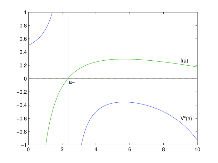
Figure 1: The wormhole is unstable whenever $a_{0}>a_{-}$.

in Fig. 1. It is clear from the figure that $V^{\prime\prime}(a_{0})<0$ whenever $a_{0}>a_{-}$, the inner horizon.

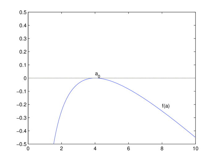
Figure 2: There is a single horizon at $a=a_{0}$.

5 Stable solutions

First we recall that for a Kiselev black hole, the Kiselev parameter is restricted to $0<\alpha\leq 1/8M$. So if $\alpha=1/8M$ and $M=1$, we obtain from Eqs. (2) and (3),

$$f(a)=1-\frac{2}{a}-\frac{a}{8},$$ (23)

yielding a single horizon at some $a=a_{0}$, shown in Fig. 2. For $\alpha>1/8M$, we obtain a naked singularity. This case yields a stable solution. (Stable solutions from naked singularities are also discussed Refs. [7] and [9].) To see why, we choose $M=1$ again. Then for an arbitrarily small $\eta>0$, we obtain a new continuous function of $a$ and $\eta$:

$$f(a,\eta)=1-\frac{2}{a}-\frac{a}{8-\eta}<0.$$ (24)

So

$$\text{lim}_{\eta\rightarrow 0}f(a_{0},\eta)=f(a_{0},0)=f(a_{0})=0.$$ (25)

Substituting in Eq. (22) with the same $\alpha$ yields another new function, this time denoted by

$$V^{\prime\prime}(a,\eta)=\frac{2}{a^{2}}\left[-\frac{2}{a}+\frac{\left(\frac{1}{a}-\frac{a}{2(8-\eta)}\right)\left(1-\frac{4}{a}\right)}{1-\frac{2}{a}-\frac{a}{8-\eta}}\right].$$ (26)

The graph of $V^{\prime\prime}(a,\eta)$, together with $f(a,\eta)$, in Fig. 3 shows two stable regions where $V^{\prime\prime}(a,\eta)>0$. Observe that $V^{\prime\prime}(a,\eta)$ is a continuous function of $a$ and $\eta$. In particular,

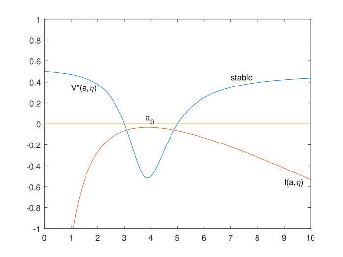
Figure 3: Plot showing the region of stability where $V^{\prime\prime}(a,\eta)>0$.

$$\text{lim}_{\eta\rightarrow 0}V^{\prime\prime}(a,\eta)=V^{\prime\prime}(a,0)=V^{\prime\prime}(a).$$ (27)

To show that one can obtain a stable solution without a naked singularity, we will use a limit argument that depends on the continuity of $V^{\prime\prime}$. Returning to Fig. 3, the two stable regions on opposite sides of $a_{0}$ begin at some value $a$, but since $\eta$ is arbitrarily small, $a$ can be placed as close to $a_{0}$ as we please. To illustrate this point, if $\eta=0.5$, then $V^{\prime\prime}=0$ at $a=3$ and $a=5$. This is the case shown in Fig. 3. If $\eta=0.1$, then the zeros of $V^{\prime\prime}$ are closer together at $a=3.55$ and $a=4.45$, respectively, and if $\eta=0.00001$, the respective zeros are at $a=3.996$ and $a=4.004$, clearly showing the trend, a shrinking interval centered at $a_{0}$. Now we can simply state that $V^{\prime\prime}>0$ outside the closed interval $[a_{0}-a,\,a_{0}+a]$. In particular, if we choose a constant $\beta>0$, then $V^{\prime\prime}(a_{0}-a-\beta,\,\eta)>0$ and $V^{\prime\prime}(a_{0}+a+\beta,\,\eta)>0$ since every $a_{0}\pm(a+\beta)$ lies outside the interval. Next, let us consider a positive sequence $\{a_{n}\}$ such that $\text{lim}_{\rightarrow\infty}a_{n}=0$. Then

$$[a_{0}-a_{n},\,a_{0}+a_{n}]\rightarrow a_{0},\,\text{to be denoted by}\,[a_{0},\,a_{0}],$$

while

$$[a_{0}-a_{n}-\beta,\,a_{0}+a_{n}+\beta]\rightarrow[a_{0}-\beta,\,a_{0}+\beta].$$

From the condition

$$V^{\prime\prime}(a_{0}\pm(a_{n}+\beta,\,\eta))>0,$$

it now follows from the continuity of $V^{\prime\prime}(a,\eta)$ that

$$\text{lim}_{n\rightarrow\infty,\,\eta\rightarrow 0}V^{\prime\prime}(a_{0}\pm(a_{n}+\beta),\,\eta)=V^{\prime\prime}(a_{0}\pm\beta,\,0)=V^{\prime\prime}(a_{0}\pm\beta),$$

making use of Eq. (27). But $V^{\prime\prime}(a_{0}\pm\beta)>0$ since every $a_{0}\pm\beta$ lies outside the interval $[a_{0},a_{0}]$. Referring to Eq. (25), since $f(a_{0},0)=f(a_{0})=0$, there is an event horizon at $a=a_{0}$ and we obtain a stable solution without a naked singularity.

We know from Sec. 2 that the special case $\alpha=1/8M$ of the Kiselev parameter yields a Schwarzschild black hole with only one event horizon, denoted by $a_{0}$ in Fig. 2. We have seen that the limiting case still fits the Kiselev model and therefore has a special significance: the thin-shell wormhole obtained is stable to linearized radial perturbations. By contrast, in Visser’s original formulation discussed in the Introduction, thin-shell wormholes are unstable if constructed directly from the traditional Schwarzschild spacetime, by which is meant a black hole that is not surrounded by quintessence dark energy [Eq. (2) with $\alpha=0$] unless the speed of sound exceeds the speed of light.

As a final comment, the region of interest in Fig. 3 is now restricted to the region on the right side since we have to remain outside the event horizon.

6 Conclusion

This paper employs the standard cut-and-paste technique for the theoretical construction of thin-shell wormholes from Kiselev black holes. Since a Kiselev black hole is surrounded by quintessence dark energy, the only reasonable equation of state for the exotic matter on the shell is the barotropic EoS $\mathcal{P}=\omega\sigma$. Most such wormholes turn out to be unstable to linearized radial perturbations. Exceptions do exist, however: by using the continuity of $V^{\prime\prime}$, it is shown by means of a limit argument that for certain choices of the parameters, stable solutions exist due to the quintessence-dark energy background. The results in this paper complement those in Refs. [3] and [4], which also deal with stable thin-shell wormholes.

References

- [1] Visser, M. Nucl. Phys. B 1989, 328, 203-212.
- [2] Morris, M. S.; Thorne, K. S. Amer. J. Phys. 1988, 56, 395-412.
- [3] Rahaman, F.; Rahman, K. A.; Rakib, Sk. A.; Kuhfittig, P. K. F. Int. J. Theor. Phys. 2010, 49, 2364-2378.
- [4] Usmani, A. A.; Rahaman, F.; Ray, S.; Rakib, Sk. A.; Kuhfittig, P. K. F. Gen. Relativ. Gravit. 2010, 42, 2901-2912.
- [5] Eiroa, E. F.; Simeone, C. Phys. Rev. D 2007, 76, 024021.
- [6] Bandyopadhyay, T.; Baveja, A.; Chakraborty, S. Int. J. Mod. Phys. D 2009, 13, 1977-1990.
- [7] Eiroa, E. F. Phys. Rev. D 2009, 80, 044033.
- [8] Sharif, M.; Azam, M. JACAP 2013, 05, 25.
- [9] Kuhfittig, P. K. F. Acta Physica Pol. B 2010, 41, 2017-2029.
- [10] Sharif, M.; Jared, F. Gen. Relativ. Gravit. 2016, 48, 158.
- [11] Kuhfittig, P. K. F. Scientific Voyage 2016, 2, 21-28.
- [12] Kiselev, V. V. Class. Quantum Grav. 2003, 20, 1187-1197.
- [13] Jiao, L.; Yang, R. Eur. Phys. J. C 2017, 77, 356.
- [14] Poisson, E.; Visser, M. Phys. Rev. D 1995, 52, 7318-7321.
- [15] Lobo, F. S. N.; Crawford, P. Class. Quantum Grav. 2004, 21, 391-404.
- [16] Eiroa, E. F.; Romero, G. E. Gen. Relativ. Gravit. 2004, 36, 651-659.
- [17] Thibeault, M.; Simeone, C.; Eiroa, E. F. Gen. Relativ. Gravit. 2006, 38, 1593-1608.
- [18] Rahaman, F.; Kalam, M.; Chakraborty, S. Gen. Relativ. Gravit. 2006, 38, 1687-1695.
- [19] Rahaman, F.; Kalam, M.; Chakraborty, S. Chin. J. Phys. 2007, 45, 518-529.
- [20] Richarte, M. G.; Simeone, C. Phys. Rev. D 2007, 76, 087502.
- [21] Lemos, J. P. S.; Lobo, F. S. N. Phys. Rev. D 2008, 78, 044030.
- [22] Younas, A.; Jamil, M.; Bahamonde, S.; Hussain, S. Phys. Rev. D 2015, 92, 084042.