Geostatistical Modeling of Positive Definite Matrices: An Application to Diffusion Tensor Imaging

Abstract

Geostatistical modeling for continuous point-referenced data has been extensively applied to neuroimaging because it produces efficient and valid statistical inference. However, diffusion tensor imaging (DTI), a neuroimaging characterizing the brain’s anatomical structure, produces a positive definite matrix for each voxel. Currently, only a few geostatistical models for positive definite matrices have been proposed because introducing spatial dependence among positive definite matrices properly is challenging. In this paper, we use the spatial Wishart process, a spatial stochastic process (random field) where each positive definite matrix-variate marginally follows a Wishart distribution, and spatial dependence between random matrices is induced by latent Gaussian processes. This process is valid on an uncountable collection of spatial locations and is almost-surely continuous, leading to a reasonable means of modeling spatial dependence. Motivated by a DTI dataset of cocaine users, we propose a spatial matrix-variate regression model based on the spatial Wishart process. A problematic issue is that the spatial Wishart process has no closed-form density function. Hence, we propose an approximation method to obtain a feasible Cholesky decomposition model and show that the Cholesky decomposition model is asymptotically equivalent to the spatial Wishart process model. A local likelihood approximation method is also applied to achieve fast computation. The simulation studies and real data analysis demonstrate that the Cholesky decomposition process model produces reliable inference and improved performance compared to other methods.

Keywords: Diffusion tensor imaging; Geostatistical modeling; Random matrix; Positive definite matrix; Spatial random fields; Spatial Wishart process; Cholesky decomposition process

1 Introduction

Diffusion tensor imaging (DTI), a magnetic resonance imaging (MRI) technique, is used to measure the diffusion process of water molecules in the brain (Soares et al., 2013). Estimated $3\times 3$ positive definite matrices summarize the water diffusion at each location in the brain. The positive definite matrix is also called a diffusion tensor (DT), representing the covariance of the local 3D Brownian motion (Schwartzman, 2006; Dryden et al., 2009). Since DTI has been used extensively to map white matter tractography in the brain, it has an advantage over other MRI-based techniques in revealing abnormal topological organization in the brain (Lo et al., 2010). A primary clinical objective is to understand how covariates (e.g., age, gender, drug use) affect DTs, reflecting its effects on brain structure.

Incorporating spatial dependence is important for achieving efficient and valid inference in imaging data analysis (Spence et al., 2007; Wu et al., 2013; Xue et al., 2018). Recently, Lan et al. (2019) also reveal that incorporating spatial dependence leads to improved performance in DTI region of difference selection, validated by an application to a cocaine user data-set (Ma et al., 2017). In point-referred data, geostatistical modeling is a useful approach. It is a class of models based on continuous spatial variation, providing a smooth surface over locations (e.g., spatial Gaussian process model). Current geostatistical modeling only focuses on random variables following univariate or multivariate distributions (e.g., univariate/multivariate Gaussian, Poisson). However, the voxel-level variable in DTI is a positive definite matrix and only a few relevant works have been proposed for spatially-varying positive definite matrices (Gelfand et al., 2004). This triggers our study of geostatistical modeling of positive definite matrices.

Previous attempts to analyze DTI data can be broadly classified into univariate modeling and matrix-variate modeling. To avoid the complexity caused by matrix-variate data, univariate modeling projects a DT onto a descriptive scalar quantity such as the magnitude of isotropy, magnitude/fractional of anisotropy, or mode of anisotropy (Ennis and Kindlmann, 2006). Among these scalar quantities, magnitude/fractional of anisotropy is the most popular (see Lane et al., 2010; Ma et al., 2017). However, since these projections are surjective (e.g., different DTs may project onto the same scalar quantity), the loss of information caused by univariate modeling is irreversible. To this end, matrix-variate modeling has been proposed via parameterizing the DTs as matrix-variate random distributions such as Wishart distribution (Dryden et al., 2009) and Gaussian random ellipsoid distribution (Schwartzman et al., 2008). However, these matrix-variate models have not yet been extended to spatial modeling because incorporating spatial dependence for positive definite matrices is non-trivial.

To mitigate these issues, we propose a spatial matrix-variate regression model. The covariates are incorporated through the Cholesky decomposition (Zhu et al., 2009), and the coefficients are spatially-varying to capture local covariate effects. The spatial dependence among positive definite matrices is achieved by the spatial Wishart process, a spatial random field (stochastic process) supporting spatially dependent Wishart matrices. The first use of the spatial Wishart process was a prior for a spatially-varying covariance matrix (Gelfand et al., 2004). In this paper, the spatial Wishart process is used as a model for positive definite matrix observations. Considering that the literature comprehensively describing the statistical properties of the spatial Wishart process is sparse, we further prove that the spatial Wishart process as a random field on uncountable locations is valid and almost-surely continuous. Although the model based on the spatial Wishart process is elegant with several nice properties, a bottleneck of the spatial Wishart process is that its probability density function is intractable (Viraswami, 1991). Therefore, instead of directly modeling the DTs, we propose a new Cholesky decomposition process model that approximates the original model by taking the Cholesky decomposition of positive definite matrices as the responses. The Cholesky decomposition process model is composed of six univariate spatial Gaussian processes, where the parameters retain the interpretations of the original model. Via theoretical results and simulation studies, we show that the Cholesky decomposition process model is an asymptotic approximation and useful working model. The theoretical results make an important contribution of both direct and potential value in applications of DTI and other fields, simplifying matrix-variate models relying on dependent Wishart matrices (e.g., Karagiannidis et al., 2003; Smith and Garth, 2007; Kuo et al., 2007) to multivariate models relying on Gaussian distributions. We also deal with massive spatial data by Vecchia’s method (Vecchia, 1988; Datta et al., 2016), a local likelihood approximation that approximates the joint density of spatial variables as a product of conditional densities. To demonstrate our proposal, we further investigate its performance using simulation studies, and provide data analysis on cocaine user data (Ma et al., 2017), in comparison to the univariate spatially-varying coefficient process model (Gelfand et al., 2003). To the best of our knowledge, this is the first work on exploring spatial associations in modeling positive definite matrix-variate data under the framework of geostatistical modeling, with some key theoretical contributions of multivariate analysis and applications to DTI.

2 Spatial Wishart Process Model

A typical DTI data set (e.g., Ma et al., 2017) usually includes DTs from each subject $i\in\{1,2,...,N\}$ at each voxel $\bm{s}\in\{\bm{s}_{1},...,\bm{s}_{n}\}$, and subject-level covariates (e.g., age, education level, medical treatments). The primary clinical objective is to detect local covariate effects on DTs. Let $\bm{A}_{i}(\bm{s})$ be the $3\times 3$ positive definite DT matrix of subject $i$ measured at voxel $\bm{s}$ and $\bm{X}_{i}$ be a design matrix containing an intercept and $d$ covariates. The positive definite DT matrices are modeled as parameterized Wishart matrices (Dryden et al., 2009) to have mean matrix $\bm{\Sigma}_{i}(\bm{s})$ and degrees of freedom $m$, denoted as $\bm{A}_{i}(\bm{s})\sim\mathcal{W}(\bm{\Sigma}_{i}(\bm{s}),m)$. To model spatial dependence and ensure that $\bm{A}_{i}(\bm{s})$ is a positive definite matrix, we decompose $\bm{A}_{i}(\bm{s})$ as

$$\bm{A}_{i}(\bm{s})=\bm{L}_{i}(\bm{s})\bm{U}_{i}(\bm{s})\bm{L}_{i}(\bm{s})^{T}.$$ (1)

In this decomposition, $\bm{U}_{i}(\bm{s})$ has mean $\bm{I}_{3}$ and is the spatially dependent residual term modeling variation which cannot be explained by the covariates and the regression term $\bm{L}_{i}(\bm{s})$ is the lower-triangle Cholesky matrix of the mean matrix $\bm{\Sigma}_{i}(\bm{s})$, i.e., $\mathbb{E}\bm{A}_{i}(\bm{s})=\bm{\Sigma}_{i}(\bm{s})=\bm{L}_{i}(\bm{s})\bm{L}_{i}(\bm{s})^{T}$. The spatial Wishart process for $\bm{U}_{i}(\bm{s})$ is described in Section 2.1 and the regression construction for $\bm{L}_{i}(\bm{s})$ as a function of $\bm{X}_{i}$ is described in Section 2.2. We refer to this model as spatial Wishart process model in the rest of the paper.

2.1 Residual Term: Spatial Wishart Process

In this subsection, we introduce the spatial Wishart process as a means of modeling spatial dependence. Gelfand et al. (2004) provide the construction of the spatial Wishart process, which is stated as follows. For $j\in\{1,2,...,m\}$, let $\{\bm{Z}_{j}(\bm{s}):\bm{s}\in\mathcal{D}\}$ be a mean-zero $p$-dimensional multivariate Gaussian process with $p\times p$ cross-covariance matrix $\bm{\Sigma}$ and spatial dependence function $\mathcal{K}(\bm{s},\bm{s}^{\prime}\mid\bm{\Phi})$ determined by parameters $\bm{\Phi}$, i.e., $cov(\bm{Z}_{j}(\bm{s}),\bm{Z}_{j}(\bm{s}^{\prime}))=\mathcal{K}(\bm{s},\bm{s}^{\prime}\mid\bm{\Phi})\times\bm{\Sigma}$, denoted as $\bm{Z}_{j}\sim\mathcal{GP}(\bm{0},\mathcal{K}(\bm{s},\bm{s}^{\prime}\mid\bm{\Phi}),\bm{\Sigma})$. If for each $\bm{s}\in\mathcal{D}$, we collect $\bm{U}(\bm{s})=\sum_{j=1}^{m}\bm{Z}_{j}(\bm{s})\bm{Z}_{j}^{T}(\bm{s})/m\sim\mathcal{W}(\bm{\Sigma},m)$, then the collection $\{\bm{U}(\bm{s}):\bm{s}\in\mathcal{D}\}$ is a spatial Wishart process, a random field supporting spatially dependent Wishart matrices. The spatial Wishart process can be understood as a two-level hierarchical model where the spatial dependence of Wishart matrix $\bm{U}(\bm{s})$ is induced by the latent spatial Gaussian processes $\{\bm{Z}_{j}\}$. Also, in light of the application to DTI, we assume $p=3$ in default.

In applications, the number of locations in $\mathcal{D}$ is usually finite. However, Gelfand et al. (2010) emphasize the importance to ensure a valid mathematical specification of a spatial stochastic process. Thus, in Theorem 1, we use the Kolmogorov extension theorem (Øksendal, 2003) to prove that it is a valid stochastic process if $\mathcal{D}$ is an uncountable collection of spatial locations (Appendix I).

Theorem 1 (Spatial Wishart Process).

The spatial Wishart process $\{\bm{U}(\bm{s}):\bm{s}\in\mathcal{D}\}$ is a valid stochastic process (random field).

Based on the fact that the random field is valid, we can also show that this field is almost-surely continuous (Property 1). The proof of almost-sure continuity is based on Kent (1989) (Appendix I).

Property 1 (Almost-Sure Continuity).

Let $\{\bm{U}(\bm{s}):\bm{s}\in\mathcal{D}\}$ be a spatial Wishart process. If the correlation function $\mathcal{K}(\bm{s},\bm{s}^{\prime}\mid\bm{\Phi})$ has a second-order Taylor series expansion with remainder that goes to $0$ at a rate of $2+\delta$ for some $\delta>0$, $\bm{U}(\bm{s})$ converges weakly to $\bm{U}(\bm{s}_{0})$ with probability one as $\mid\mid\bm{s}-\bm{s}_{0}\mid\mid\rightarrow 0$.

Considering that neuroimaging data is usually is collected at a high resolution and the disease status at proximally-located/neighboring voxels can be similar (see Wu et al., 2013; Xue et al., 2018), the residuals $\bm{U}_{i}(\bm{s})$ should be smooth and spatially dependent. Therefore, we model the residuals $\{\bm{U}_{i}(\bm{s}):\bm{s}\in\mathcal{D}\}$ for $i\in\{1,2,...,N\}$ as realizations of a spatial Wishart process with degrees of freedom $m$, cross-covariance matrix $\bm{I}$, and correlation function $\mathcal{K}(\bm{s},\bm{s}^{\prime}\mid\bm{\Phi})$, denoted as

$$\bm{U}_{i}\sim\mathcal{SWP}(m,\mathcal{K}(\bm{s},\bm{s}^{\prime}\mid\bm{\Phi}),\bm{I}).$$ (2)

Setting the cross-covariance matrix to $\bm{I}$ preserves the designed marginal distribution $\bm{A}_{i}(\bm{s})\sim\mathcal{W}(\bm{\Sigma}_{i}(\bm{s}),m)$.

In spatial statistics and neuroimaging, understanding the spatial dependence is essential. We quantify spatial dependence of the spatial Wishart process using the expected squared Frobenius norm $\mathcal{V}(\bm{s},\bm{s}^{\prime})=\mathbb{E}\mid\mid\bm{U}(\bm{s})-\bm{U}(\bm{s}^{\prime})\mid\mid_{F}^{2}$, where $\mid\mid.\mid\mid_{F}$ is the Frobenius norm. The expected squared Frobenius norm can also be understood as a generalized variogram (Cressie, 1992) for matrix-variate data (Lan et al., 2019), where an increasing spatial dependence of $\bm{U}(\bm{s})$ and $\bm{U}(\bm{s}^{\prime})$ leads to a smaller $\mathcal{V}(\bm{s},\bm{s}^{\prime})$. Through the variogram, we find that the spatial Wishart process $\mathcal{SWP}(m,\mathcal{K}(\bm{s},\bm{s}^{\prime}\mid\bm{\Phi}),\bm{\Sigma})$ is separable (Cressie, 1992) since

$$\mathcal{V}(\bm{s},\bm{s}^{\prime})=\gamma(m,\bm{\Sigma})[1-\mathcal{K}(\bm{s},\bm{s}^{\prime}\mid\bm{\Phi})^{2}],$$ (3)

where the term $1-\mathcal{K}(\bm{s},\bm{s}^{\prime}\mid\bm{\Phi})^{2}$ is the spatial term and $\gamma(m,\bm{\Sigma})=\frac{2}{m}Tr(\bm{\Sigma\Sigma})+\frac{2}{m}Tr(\bm{\Sigma})Tr(\bm{\Sigma})$ is the non-spatial term. The property of spatial separability makes the residual variation more transparent: The cross-dependence of positive definite matrices depends on $\gamma(m,\bm{\Sigma})$ such that an increasing $m$, primarily controlling the variance of a Wishart matrix, leads to smaller cross-dependence; A larger spatial correlation of the underlying Gaussian processes leads to larger spatial dependence.

The spatial dependence can be visualized via realizations of the standard spatial Wishart processes ($\bm{\Sigma}=\bm{I}$) on a $20\times 20$ grid with spacing of 1 between adjacent grid points. Given the spatial correlation function is exponential $\mathcal{K}(\bm{s},\bm{s}^{\prime}\mid\rho)=\exp\left[-\frac{\mid\mid\bm{s}-\bm{s}^{\prime}\mid\mid}{\rho}\right]$, we visualize the positive definite matrices in two dimensions as ellipsoids in Figure 1. In Figure 1(a), the positive definite matrices are simulated with $m=3$ and $\rho=1,4,10$, where a larger $\rho$ leads to stronger spatial dependence; In Figure 1(b), positive definite matrices are simulated with $\rho=4$ and $m=3,6,10$, where a larger $m$ leads smaller cross-dependence. Since the three cases in Figure 1(b) maintain the same level of spatial dependence, we may also identify that the spatial and non-spatial variations are separable.

(a) Simulated positive definite matrices with $m=10$.

(b) Simulated positive definite matrices with $\rho=4$.

Figure 1: Simulated positive definite matrices from standard spatial Wishart processes, i.e., with mean equal to the identity matrix. The spatial dependence of positive definite matrices depends on the range parameter $\rho$. The cross-dependence of positive definite matrices depends on the degrees of freedom $m$.

2.2 Regression Term: Cholesky Decomposition

Expressing the mean matrix $\bm{\Sigma}_{i}(\bm{s})$ in terms of $\bm{X}_{i}$ is not straightforward (Zhu et al., 2009; Yuan et al., 2012) because the responses $\bm{A}_{i}(\bm{s})$ are in a Remannian manifold but the covariates $\bm{X}_{i}$ are in Euclidean space. Following Zhu et al. (2009), we regress the $(k,l)$-th element of $\bm{L}_{i}(\bm{s})$, denoted as $l_{ikl}(\bm{s})$ on $\bm{X}_{i}$ as

$$\log l_{ikk}(\bm{s})=\bm{X}_{i}\bm{\beta}_{kk}(\bm{s}),\quad l_{ikl}(\bm{s})=\bm{X}_{i}\bm{\beta}_{kl}(\bm{s})\quad\text{for $k>l$},$$ (4)

where $\bm{\beta}_{kl}(\bm{s})=[\beta_{0kl}(\bm{s}),\beta_{1kl}(\bm{s}),...,\beta_{dkl}(\bm{s})]^{T}$ is the spatially-varying coefficient vector and $\beta_{jkl}(\bm{s})$ is the coefficient associated with the $j$-th covariate. The roles of the coefficients $\bm{\beta}_{kl}(\bm{s})$ can be explained as linear effect on $\log l_{ikk}(\bm{s})$ or $l_{ikl}(\bm{s})$. To model the spatial dependence of the mean effect, we assign a mean-zero spatial Gaussian process prior on $\bm{\beta}(\bm{s})=[\bm{\beta}_{11}(\bm{s})^{T},\bm{\beta}_{22}(\bm{s})^{T},\bm{\beta}_{33}(\bm{s})^{T},\bm{\beta}_{21}(\bm{s})^{T},\bm{\beta}_{31}(\bm{s})^{T},\bm{\beta}_{32}(\bm{s})^{T}]^{T}$, denoted as $\bm{\beta}\sim\mathcal{GP}(\bm{0},\mathcal{K}(\bm{s},\bm{s}^{\prime}\mid\bm{\Phi}_{\beta}),\sigma_{\beta}^{2}\bm{I})$, where $\bm{\Phi}_{\beta}$ is a set of spatial parameters controlling the spatial dependence of mean process, and $\sigma_{\beta}^{2}$ is the variance of the Gaussian process.

3 Cholesky Decomposition Process Model

Viraswami (1991) and others (e.g., Blumenson and Miller, 1963; Smith and Garth, 2007) show that a closed-form probability density function of the spatial Wishart process model is available if the latent spatial precision matrix is tri-diagonal. However, the joint probability density function of multiple locations is not appropriate to be used for large-scale spatial modeling because this assumption of tri-diagonal precision matrix is unrealistic in spatial modeling. Therefore, to approximate the spatial Wishart process model, we further propose the Cholesky decomposition process model. The Cholesky decomposition process model is specified on the Cholesky decomposition elements of $\bm{A}_{i}(\bm{s})$, denoted as $\{t_{ikl}(\bm{s}):k\geq l,\bm{s}\in\mathcal{D}\}$. The model is

Diagonal: $$\sqrt{2}\log t_{ikk}\sim\mathcal{GP}\left(\sqrt{2}\bm{X}_{i}\bm{\beta}_{kk}(\bm{s}),\mathcal{C}(\bm{s},\bm{s}^{\prime}\mid\bm{\Phi}_{u}),\sigma_{m}^{2}\right) \text{for $k=1,2,3$},$$ (5)

Off-Diagonal: $$t_{{ikl}}\mid\bar{t}_{ikk}\sim\mathcal{GP}(\bm{X}_{i}\bm{\beta}_{kl}(\bm{s}),\mathcal{C}(\bm{s},\bm{s}^{\prime}\mid\bm{\Phi}_{u})\bar{t}_{ikk}(\bm{s})\bar{t}_{ikk}(\bm{s}^{\prime}),\sigma_{m}^{2}) \text{for $k>l$},$$

In this expression, $\sqrt{2}\bm{X}_{i}\bm{\beta}_{kk}(\bm{s})$ and $\bm{X}_{i}\bm{\beta}_{kl}(\bm{s})$ are marginal means of the diagonal and off-diagonal Gaussian processes at location $\bm{s}$, respectively. Also, $\bar{t}_{ikk}(\bm{s})=\exp(\bm{X}_{i}\hat{\bm{\beta}}_{kk}(\bm{s}))$ and $\hat{\bm{\beta}}_{kk}(\bm{s})$ is the ordinary least squares estimates computed using only data at voxel $\bm{s}$ from regressing $\log t_{ikk}(\bm{s})$ on $\bm{X}_{i}$.

To provide a rigorous mathematical validation, we also prove that $\{\bm{A}_{i}(\bm{s})=\bm{T}_{i}(\bm{s})\bm{T}_{i}(\bm{s})^{T}:\bm{s}\in\mathcal{D}\}$ is a valid stochastic process and almost-surely continuous (Theorem 2), where $\bm{T}_{i}(\bm{s})$ is the lower-triangle Cholesky matrix.

Theorem 2 (Cholesky Decomposition Process).

$\{\bm{A}_{i}(\bm{s})=\bm{T}_{i}(\bm{s})\bm{T}_{i}(\bm{s})^{T}:\bm{s}\in\mathcal{D}\}$ is a valid stochastic process. Also, if the correlation function $\mathcal{C}(\bm{s},\bm{s}^{\prime}\mid\bm{\Phi})$ has a second-order Taylor series expansion with remainder that goes to $0$ at a rate of $2+\delta$ for some $\delta>0$, $\bm{A}(\bm{s})$ converges weakly to $\bm{A}(\bm{s}_{0})$ with probability one as $\mid\mid\bm{s}-\bm{s}_{0}\mid\mid\rightarrow 0$.

To link to the spatial Wishart process model, we assume that $\mathcal{C}(\bm{s},\bm{s}^{\prime}\mid\bm{\Phi}_{u})=\mathcal{K}(\bm{s},\bm{s}^{\prime}\mid\bm{\Phi}_{u})^{2}$ and $\sigma_{m}^{2}=\frac{1}{m}$. Given the asymptotic properties in Theorem 3, we may conclude that asymptotically the two models are equivalent and the parameters in the two models have the same interpreations: $\bm{\beta}_{kk}(\bm{s})$ controls the mean of $\log t_{ikk}(\bm{s})$ and partially describes local variation of $t_{ikl}(\bm{s})$; $\bm{\beta}_{kl}(\bm{s})$ controls the mean of $t_{ikl}(\bm{s})$; $\bm{\Phi}_{u}$ controls the spatial residual dependence. Furthermore, if we modify that $\bar{t}_{ikk}(\bm{s})=\exp(\bm{X}_{i}{\bm{\beta}}_{kk}(\bm{s}))$ in (5), the condition that $N\rightarrow\infty$ can be omitted to show that $\{\sqrt{m}[e_{ikl}(\bm{s}_{1}),...,e_{ikl}(\bm{s}_{n})]^{T}\mid\bm{S}_{e_{ikl}}\}$ converges in distribution to $\{\sqrt{m}[t_{ikl}(\bm{s}_{1}),...,t_{ikl}(\bm{s}_{n})]^{T}\mid\bar{t}_{ikk}\}$. However, we show that the specification in (5) leads to computationally efficient Gibbs sampling for coefficients (Section 3.1) and a reasonable trade-off according to the simulation results showing the closeness of parameter estimation (Section 4).

Theorem 3 (Asymptotic Properties).

For $i\in\{1,2,...,N\}$, let $\{t_{ikl}(\bm{s}):k\geq l,\bm{s}\in\mathcal{D}\}$ and $\{e_{ikl}(\bm{s}):k\geq l,\bm{s}\in\mathcal{D}\}$ be Cholesky decomposition elements of $\{\bm{A}_{i}(\bm{s}):\bm{s}\in\mathcal{D}\}$ following the Cholesky decomposition process model and the spatial Wishart process model, respectively. For $\bm{s}_{1},...,\bm{s}_{n}\in\mathcal{D}$, we have the following asymptotic results:

• Diagonal: As $m\rightarrow\infty$, $\sqrt{m}[\log e_{ikk}(\bm{s}_{1})-\bm{X}_{i}\bm{\beta}_{kk}(\bm{s}_{1}),...,\log e_{ikk}(\bm{s}_{n})-\bm{X}_{i}\bm{\beta}_{kk}(\bm{s}_{n})]^{T}$ converges in distribution to $\sqrt{m}[\log t_{ikk}(\bm{s}_{1})-\bm{X}_{i}\bm{\beta}_{kk}(\bm{s}_{1}),...,\log t_{ikk}(\bm{s}_{n})-\bm{X}_{i}\bm{\beta}_{kk}(\bm{s}_{n})]^{T}$ for $k=1,2,3$;
  

• Off-Diagonal:

  • Let $\bm{\mu}_{m,kl}$ (dependent of $m$) and $\bm{\mu}_{kl}$ (independent of $m$) be the means of $\{[e_{ikl}(\bm{s}_{1}),...,e_{ikl}(\bm{s}_{n})]^{T}|\bm{S}_{e_{ikl}}\}$ and $\{[t_{ikl}(\bm{s}_{1}),...,t_{ikl}(\bm{s}_{n})]^{T}|\bar{t}_{ikk}\}$, respectively. As $m\rightarrow\infty$, $\bm{\mu}_{m,kl}$ converges in probability to $\bm{\mu}_{kl}$, and $cor(e_{{ikl}}(\bm{s}),e_{{ikl}}(\bm{s}^{\prime})\mid\bm{S}_{e_{ikl}})$ converges in probability to $cor(t_{{ikl}}(\bm{s}),t_{{ikl}}(\bm{s}^{\prime})\mid\bar{t}_{ikk})=\mathcal{K}(\bm{s},\bm{s}^{\prime}\mid\bm{\Phi})^{2}=\mathcal{C}(\bm{s},\bm{s}^{\prime}\mid\bm{\Phi})$;

  • If $\bm{\beta}_{kl}(\bm{s})=\bm{0}$ for all $\bm{s}\in\mathcal{D}$ and $k>l$, then as $m\rightarrow\infty$ and $N\rightarrow\infty$, $\{\sqrt{m}[e_{ikl}(\bm{s}_{1}),...,e_{ikl}(\bm{s}_{n})]^{T}\mid\bm{S}_{e_{ikl}}\}$ converges in distribution to $\{\sqrt{m}[t_{ikl}(\bm{s}_{1}),...,t_{ikl}(\bm{s}_{n})]^{T}\mid\bar{t}_{ikk}\}$, for $k>l$;

  • If $\bm{\beta}_{kl}(\bm{s})=\bm{0}$ for all $\bm{s}\in\mathcal{D}$ and $k>l$, and that $\bar{t}_{ikk}(\bm{s})=\exp(\bm{X}_{i}{\bm{\beta}}_{kk}(\bm{s}))$, then as $m\rightarrow\infty$, $\{\sqrt{m}[e_{ikl}(\bm{s}_{1}),...,e_{ikl}(\bm{s}_{n})]^{T}\mid\bm{S}_{e_{ikl}}\}$ converges in distribution to $\{\sqrt{m}[t_{ikl}(\bm{s}_{1}),...,t_{ikl}(\bm{s}_{n})]^{T}\mid\bar{t}_{ikk}\}$, for $k>l$;

$\bm{S}_{e_{ikl}}(\bm{s})$ is a partition of the latent Gaussian processes defined in spatial Wishart process i.e., $\{\bm{Z}_{ij}(\bm{s})=[{Z}_{ij1}(\bm{s}),{Z}_{ij2}(\bm{s}),{Z}_{ij3}(\bm{s})]^{T}:\bm{s}\in\mathcal{D}\}$ for $j\in\{1,2,...,m\}$ ($i$ is a fixed and given index here. The partition is to take the dimensions “above” of $e_{ikl}$ such as $\{[{Z}_{ij1}(\bm{s}),...,{Z}_{ij(k-1)}(\bm{s})]^{T}:\bm{s}\in\mathcal{D}\}$ for all $j$. For example, $\bm{S}_{e_{i31}}$ or $\bm{S}_{e_{i32}}$ is $\{[{Z}_{ij1}(\bm{s}),{Z}_{ij2}(\bm{s})]^{T}:\bm{s}\in\mathcal{D}\}$ for all $j$, and $\bm{S}_{e_{i21}}(\bm{s})$ is $\{{Z}_{ij1}(\bm{s}):\bm{s}\in\mathcal{D}\}$ for all $j$.

The asymptotic results apply for large degrees of freedom, $m$. In both models, large m corresponds to small residual variability, i.e., images with small noise. This is a reasonable condition in our motivating data (see Section 5) where the estimated residual variance is small. In comparison to the spatial Wishart process model, the Cholesky decomposition process model is a more computational convenient Gaussian processes. Moreover, since the underlying mechanism of the DT’s spatial dependence is unknown, both models can be treated as proposed geostatistical models for DTI. All the proofs for the results in this section are summarized in Appendix II.

3.1 Computational Details

In this subsection, we give the computational details of this model. We fit the model using Markov chain Monte Carlo and assign weakly informative priors to parameters. Given that $\mathcal{K}$ is the Matern correlation function, we define $\rho_{u},\nu_{u}\in\bm{\Phi}_{u}$ as the range and smoothness parameter of the residual dependence, and $\rho_{\beta},\nu_{\beta}\in\bm{\Phi}_{\beta}$ as the range and smoothness parameter of the mean dependence. We give priors to these parameters: $\log\rho_{u}$ and $\log\rho_{\beta}$ follow a normal distribution with mean $0$ and standard deviation $1$; $\log\nu_{u}$ and $\log\nu_{\beta}$ follow a normal distribution with mean $-1$ and standard deviation $1$; $\sigma_{\beta}^{-2}$ and $\sigma_{m}^{-2}$ follow a gamma distribution with shape $0.01$ and rate $0.01$, which are conjugate priors allowing Gibbs sampling. The coefficients $\bm{\beta}$ are also updated using Gibbs sampling because their full conditional distributions are Gaussian distributions.

The computational bottleneck of the Cholesky decomposition process model is factoring the large $n\times n$ covariance matrix of the residual dependence and mean dependence, known as the $\mathcal{O}(n^{3})$ problem in spatial statistics (e.g., Heaton et al., 2018). We address this problem using Vecchia’s method (Vecchia, 1988), a local likelihood approximation that approximates the joint density of spatial variables as a product of conditional densities. Let $\omega$ be an arbitrary Gaussian process. The approximate joint density is $p[w(\bm{s}_{1}),...,w(\bm{s}_{n})]=\prod_{i=1}^{n}p[w(\bm{s}_{i})\mid w(\bm{s}_{k}),\bm{s}_{k}\in N(\bm{s}_{i})]$, where $N(\bm{s}_{i})$ is a set of neighboring locations of $\bm{s}_{i}$ (Datta et al., 2016). This reduces the computational complexity from $\mathcal{O}(n^{3})$ to $\mathcal{O}(nq^{3})$, where $q\ll n$ is the largest size of $N(\bm{s})$. This approximation is implemented for $t_{ikl}$, $\log t_{ikk}$, and $\bm{\beta}$, where lexicographical order of locations on the regular spatial grid is used and $N(\bm{s}_{i})$ is the following $q$ locations with larger ranks. A sensitivity analysis is presented in Section 4 to investigate the impact of the tuning parameter $q$ on the Cholesky decomposition process model.

4 Simulation

In this section, we first investigate the performance of the Cholesky decomposition process model under data generated from either the spatial Wishart process or Cholesky decomposition process model, demonstrating that the Cholesky decomposition process model produces reliable results under different geostatistical settings. Also, since we apply Vecchia’s approximation for fast computation, we conduct a sensitivity analysis to investigate the impact of $q$ on parameter estimation.

For both models, we generate the synthetic DTs on $20\times 20$ grids with spacing of 1 between adjacent grid points. To mimic a real DTI study, $N=10$ subjects are simulated with drug-use indicator $x_{i,drug}\in\{0,1\}$ and normalized age $x_{i,age}\in\mathbb{R}^{+}$. The simulation study involves 50 replications. For each replication, there are $5$ drug users ($x_{i,drug}=1$) and $5$ non-drug users ($x_{i,drug}=0$), and $x_{i,age}$ is generated by a positive half-normal distribution (Leone et al., 1961) with mean $0$ and variance $1$. For each replication, all the coefficients $\bm{\beta}$ are generated from a spatial Gaussian process with variance $\sigma_{\beta}=0.1$ and correlation function $\mathcal{K}(\bm{s},\bm{s}^{\prime}\mid\bm{\Phi}_{\beta})$. The Gaussian process mean for three covariates (Table 1) simulates a scenario that drug has an effect on certain regions of the brain and increasing age may affect the whole brain. In all replications, we simulate the data with $\rho_{u}=\rho_{\beta}=2$, $\nu_{u}=\nu_{\beta}=0.5$, and $m=50$. To investigate if Vecchia’s approximation with different $q$ affects the model performance, we set $q=10,50$ and compare it to the model without Vecchia’s approximation. For each replication, we collect 5,000 Markov chain Monte Carlo samples after discarding 2,000 samples as burn-in.

Table 1: The spatial Gaussian process mean of the six coefficient vector for three covariates are summarized. $\mathcal{S}$ is a set of spatial locations inside a $4\times 4$ region in the middle of the image.

Covariate	Diagonal	Off-Diagonal
Intercept	$\beta_{int,kk}=0,\ \forall\bm{s}$	$\beta_{int,kk}=0,\ \forall\bm{s}$
$x_{i,drug}$	$\beta_{drug,kk}=0.5,\ \text{for}\bm{s}\in\mathcal{S}$ $\beta_{drug,kk}=0,\ \text{for}\bm{s}\notin\mathcal{S}$	$\beta_{drug,kl}=0,\ \forall\bm{s}$
$x_{i,age}$	$\beta_{kk,age}=0.25,\ \forall\bm{s}$	$\beta_{kl,age}=0.25,\ \forall\bm{s}$

The simulation results in terms of mean absolute deviation of posterior mean estimates, $95\%$ posterior coverage, and Monte Carlo standard deviation are summarized in Tables 2 and 3. To have a concise presentation, the values about coefficient estimates (Table 2) are averaged over replications, voxels ($n$), and covariates ($d$). From the simulation result, we find that Vecchia’s approximation is acceptable since the computational times are 6 hours, 11 hours, and 35 hours for models with 10 neighbors, 50 neighbors, and without Vecchia’s approximation and the mean absolute deviation is nearly identical for all the three methods. We further conduct simulations with $m=3$ (Table 4 and 5). When the degrees of freedom $m$ are large, the theoretical asymptotic results (Theorem 3) apply because the parameter estimations are close. Otherwise, when the degrees of freedom $m$ are small, the theoretical asymptotic results (Theorem 3) does not apply and inflated coverage is found when data is generated from the SWP model.

Table 2: Asymptotic ($m=50$) simulation results for spatially-varying coefficients with the data generated from the Cholesky decomposition process model or the spatial Wishart process model. The results are summarized in terms of mean absolute deviation of posterior mean estimates, $95\%$ posterior coverage, and Monte Carlo standard deviation. The values are averaged over replications, voxels ($n$), and covariates ($d$).

Parameter	$q$	MAD		Coverage $95\%$		MCSD
		CDP	SWP	CDP	SWP	CDP	SWP
$\bm{\beta}_{11}$	10	0.104	0.104	$95\%$	$93\%$	0.05	0.05
	50	0.104	0.104	$95\%$	$95\%$	0.05	0.05
	Standard	0.104	0.094	$95\%$	$96\%$	0.05	0.06
$\bm{\beta}_{22}$	10	0.103	0.103	$94\%$	$95\%$	0.05	0.05
	50	0.103	0.103	$94\%$	$95\%$	0.05	0.06
	Standard	0.104	0.092	$91\%$	$95\%$	0.05	0.05
$\bm{\beta}_{33}$	10	0.104	0.104	$94\%$	$94\%$	0.05	0.05
	50	0.105	0.104	$93\%$	$96\%$	0.05	0.05
	Standard	0.105	0.092	$93\%$	$97\%$	0.05	0.06
$\bm{\beta}_{21}$	10	0.107	0.097	$97\%$	$99\%$	0.08	0.07
	50	0.110	0.097	$97\%$	$97\%$	0.08	0.08
	Standard	0.107	0.096	$93\%$	$97\%$	0.07	0.08
$\bm{\beta}_{31}$	10	0.109	0.097	$95\%$	$99\%$	0.07	0.07
	50	0.110	0.096	$95\%$	$95\%$	0.07	0.08
	Standard	0.109	0.096	$95\%$	$99\%$	0.07	0.08
$\bm{\beta}_{32}$	10	0.109	0.097	$95\%$	$99\%$	0.08	0.08
	50	0.111	0.097	$95\%$	$99\%$	0.08	0.08
	Standard	0.109	0.097	$95\%$	$97\%$	0.07	0.08
MAD: Mean Absolute Deviation;
MCSD: Monte Carlo Standard Deviation;
SWP: Spatial Wishart Process Model;
CDP: Cholesky Decomposition Process Model.

Table 3: Asymptotic ($m=50$) simulation results for spatial parameters with the data generated from the Cholesky decomposition process model or the spatial Wishart process model. The results are summarized in terms of mean absolute deviation of posterior mean estimates, $95\%$ posterior coverage, and Monte Carlo standard deviation. The values are averaged over replications.

Parameter	$q$	MAD		Coverage $95\%$		MCSD
		CDP	SWP	CDP	SWP	CDP	SWP
$\rho_{u}=2$	10	0.17	0.20	$98\%$	$98\%$	0.15	0.19
	50	0.17	0.20	$96\%$	$96\%$	0.16	0.19
	Standard	0.10	0.14	$98\%$	$96\%$	0.16	0.20
$\nu_{u}=0.5$	10	0.033	0.033	$98\%$	$98\%$	0.035	0.027
	50	0.033	0.033	$98\%$	$98\%$	0.032	0.029
	Standard	0.022	0.022	$97\%$	$96\%$	0.040	0.031
$\rho_{\beta}=2$	10	0.13	0.13	$98\%$	$98\%$	0.20	0.25
	50	0.13	0.13	$98\%$	$98\%$	0.20	0.24
	Standard	0.10	0.13	$98\%$	$98\%$	0.21	0.25
$\nu_{\beta}=0.5$	10	0.038	0.038	$96\%$	$96\%$	0.040	0.050
	50	0.038	0.038	$96\%$	$98\%$	0.044	0.052
	Standard	0.038	0.058	$98\%$	$96\%$	0.043	0.053
MAD: Mean Absolute Deviation;
MCSD: Monte Carlo Standard Deviation;
SWP: Spatial Wishart Process Model;
CDP: Cholesky Decomposition Process Model.

Table 4: Non-asymptotic ($m=3$) simulation results for spatially-varying coefficients with the data generated from the Cholesky decomposition process model or the spatial Wishart process model. The results are summarized in terms of mean absolute deviation of posterior mean estimates, $95\%$ posterior coverage, and Monte Carlo standard deviation. The values are averaged over replications, voxels ($n$), and covariates ($d$).

Parameter	$q$	MAD		Coverage $95\%$		MCSD
		CDP	SWP	CDP	SWP	CDP	SWP
$\bm{\beta}_{11}$	10	0.23	0.61	$93\%$	$100\%$	0.22	0.75
	50	0.22	0.60	$95\%$	$100\%$	0.21	0.75
	Standard	0.22	0.58	$96\%$	$100\%$	0.22	0.78
$\bm{\beta}_{22}$	10	0.22	0.74	$95\%$	$100\%$	0.22	0.75
	50	0.22	0.72	$95\%$	$100\%$	0.23	0.75
	Standard	0.22	0.70	$95\%$	$100\%$	0.22	0.75
$\bm{\beta}_{33}$	10	0.23	1.06	$94\%$	$100\%$	0.22	0.75
	50	0.23	0.95	$92\%$	$100\%$	0.23	0.76
	Standard	0.22	0.92	$93\%$	$100\%$	0.23	0.75
$\bm{\beta}_{21}$	10	0.22	0.12	$99\%$	$100\%$	0.24	0.18
	50	0.23	0.13	$97\%$	$100\%$	0.24	0.15
	Standard	0.23	0.13	$94\%$	$100\%$	0.23	0.17
$\bm{\beta}_{31}$	10	0.23	0.24	$99\%$	$100\%$	0.22	0.17
	50	0.22	0.15	$95\%$	$100\%$	0.23	0.13
	Standard	0.12	0.15	$96\%$	$100\%$	0.23	0.17
$\bm{\beta}_{32}$	10	0.23	0.19	$99\%$	$100\%$	0.22	0.19
	50	0.23	0.19	$99\%$	$100\%$	0.23	0.18
	Standard	0.22	0.19	$93\%$	$100\%$	0.24	0.18
MAD: Mean Absolute Deviation;
MCSD: Standard Deviation;
SWP: Spatial Wishart Process Model;
CDP: Cholesky Decomposition Process Model.

Table 5: Non-asymptotic ($m=3$) simulation results for spatial parameters with the data generated from the Cholesky decomposition process model or the spatial Wishart process model. The results are summarized in terms of mean absolute deviation of posterior mean estimates, $95\%$ posterior coverage, and Monte Carlo standard deviation. The values are averaged over replications.

Parameter	$q$	MAD		Coverage $95\%$		MCSD
		CDP	SWP	CDP	SWP	CDP	SWP
$\rho_{u}=2$	10	0.20	0.68	$98\%$	$98\%$	0.19	0.61
	50	0.20	0.66	$96\%$	$100\%$	0.19	0.62
	Standard	0.14	0.66	$94\%$	$98\%$	0.20	0.60
$\nu_{u}=0.5$	10	0.033	0.23	$98\%$	$100\%$	0.027	0.056
	50	0.033	0.24	$98\%$	$100\%$	0.029	0.055
	Standard	0.022	0.22	$96\%$	$100\%$	0.031	0.055
$\rho_{\beta}=2$	10	0.13	0.63	$98\%$	$100\%$	0.25	0.59
	50	0.13	0.53	$93\%$	$100\%$	0.24	0.59
	Standard	0.10	0.53	$95\%$	$100\%$	0.24	0.58
$\nu_{\beta}=0.5$	10	0.038	0.23	$96\%$	$100\%$	0.050	0.055
	50	0.038	0.24	$94\%$	$100\%$	0.052	0.054
	Standard	0.058	0.23	$96\%$	$100\%$	0.053	0.055
MAD: Mean Absolute Deviation;
MCSD: MCStandard Deviation;
SWP: Spatial Wishart Process Model;
CDP: Cholesky Decomposition Process Model.

Next, we compare the performance of the Cholesky decomposition process model and the univariate spatially-varying coefficient model (Gelfand et al., 2003). In clinical studies and neuroimaging, the most interesting covariate effect is the drug-use effect ($x_{i,drug}$) (Brick and Erickson, 1998). The six coefficients comprehensively but not concisely describe the local covariate effects, which may not be affirmative to clinicians who prefer scalar quantities (e.g., fractional anisotropy). However, since the six coefficients capture the covariate effects without information loss, our method can accurately project the information onto any clinically meaningful scalar quantity. One of the useful quantities is fractional anisotropy, projecting a positive definite matrix onto $[0,1]$, defined as

$${\displaystyle{f_{FA}(\bm{A}})={\sqrt{\frac{1}{2}}}{\frac{\sqrt{(\lambda_{1}-\lambda_{2})^{2}+(\lambda_{2}-\lambda_{3})^{2}+(\lambda_{3}-\lambda_{1})^{2}}}{\sqrt{\lambda_{1}^{2}+\lambda_{2}^{2}+\lambda_{3}^{2}}}}},$$ (6)

where $\{\lambda_{1},\lambda_{2},\lambda_{3}\}$ are the eigenvalues of a diffusion tensor $\bm{A}$ (Ennis and Kindlmann, 2006). To demonstrate this, we estimate the treatment effect of cocaine use on each voxel $\bm{s}$ in terms of fractional anisotropy, denoted as $\delta_{FA}(\bm{s})=f_{FA}(\bm{\Sigma}^{(1)}({\bm{s}}))-f_{FA}(\bm{\Sigma}^{(0)}({\bm{s}}))$. Assuming $\bm{X}_{i}^{\prime}$ as the covariates excluding drug use, the term $\bm{\Sigma}^{(d)}({\bm{s}})=\frac{1}{N}\sum_{i=1}^{N}\mathbb{E}[\bm{\Sigma}(\bm{s})\mid\bm{X}_{i}^{\prime},x_{drug}=d]$ is to describe the averaged (over subjects) mean matrix at voxel $\bm{s}$ under drug-use status $d\in\{0,1\}$. We use a Markov chain Monte Carlo-based outcome regression estimator (Rotnitzky et al., 1998) to estimate $\delta_{FA}(\bm{s})$, defined as

$$\hat{\delta}_{FA}(\bm{s})=\frac{1}{N}\sum_{i=1}^{N}\left(\mathbb{E}[f_{FA}[\bm{\Sigma}_{i}(\bm{s})]\mid\bm{x}_{i,drug}=1,rest]-\mathbb{E}[f_{FA}[\bm{\Sigma}_{i}(\bm{s})]\mid\bm{x}_{i,drug}=0,rest]\right),$$ (7)

where the expectation can be empirically obtained by Markov chain Monte Carlo samples.

Since the spatial matrix-variate methods in terms of coefficients estimation have consistent results, we simply use the results of the Cholesky decomposition process model with $q=10$ and $m=50$ for a concise illustration. We plot the posterior means of $\delta_{FA}(\bm{s})$ in Figure 2, combining all voxels $\bm{s}$ and replications. We compare it to the univariate spatially-varying coefficient model (Gelfand et al., 2003) with logit transformation of fractional anisotropy as responses and its associated Markov chain Monte Carlo-based outcome regression estimator (Rotnitzky et al., 1998) is

$$\hat{\delta}_{FA}(\bm{s})=\frac{1}{N}\sum_{i=1}^{N}\left(\mathbb{E}[f_{logit}^{-1}[y_{i}(\bm{s})]\mid\bm{x}_{i,drug}=1,rest]-\mathbb{E}[f_{logit}^{-1}[y_{i}(\bm{s})]\mid\bm{x}_{i,drug}=0,rest]\right),$$ (8)

where $y_{i}(\bm{s})$ is response and $f_{logit}$ is the logit transformation. In Figure 2, the Cholesky decomposition process model produces more precise estimates for $\delta_{FA}(\bm{s})$ for $\bm{s}\in\mathcal{S}$ with smaller uncertainties, revealing that utilizing the whole matrix information plays a key role in detecting covariate effects. This claim is further verified in real data analysis (see Figure 6).

(a) $\delta_{FA}(\bm{s})$ for $\bm{s}\in\mathcal{S}$.

(b) $\delta_{FA}(\bm{s})$ for $\bm{s}\notin\mathcal{S}$

Figure 2: Estimates of $\delta_{FA}(\bm{s})$ produces by the Cholesky decomposition process model and the univariate model. The red dashed lines are the true values. $\mathcal{S}$ is a set of spatial locations inside a $4\times 4$ region in the middle of the image.

5 Application to the Cocaine User Data

In this section, we apply the model to a data set of cocaine users (Ma et al., 2017). The data are provided by the Institute for Drug and Alcohol Studies of Virginia Commonwealth University (VCU). Eleven cocaine users and eleven non-cocaine users participated in this study. Besides their cocaine-use status, their age and education years are also recorded. Following the conventions in cocaine use studies (e.g., Lane et al., 2010; Ma et al., 2017), we focus on the corpus callosum, a brain region playing important roles such as transferring motor, sensory, and cognitive information between the brain hemispheres. This region contains $15,273$ voxels.

We first fit the data to the Cholesky decomposition process model to investigate the covariate effects and spatial dependence among voxels. We set the design matrix $\bm{X}_{i}$ as $[1,x_{i,drug},x_{i,age},x_{i,edu},x_{i,handedness},x_{gender}]$, representing the intercept, drug-use ($x_{i,drug}=1$ if subject $i$ is a cocaine user, otherwise $x_{i,drug}=0$), age, education years, handedness ($x_{i,handedness}=1$ if subject $i$ is a left-handed, otherwise $x_{i,handedness}=0$), and gender ($x_{i,gender}=1$ if subject $i$ is female, otherwise $x_{i,gender}=0$). We set $q=50$ for Vecchia’s approximation and totally $8,000$ Markov chain Monte Carlo samples are collected after $3,000$ samples as burn-in.

To understand the spatial dependence of the DTs, we plot the posterior density of the spatial dependence parameters $\rho_{u}$, $\nu_{u}$, $\rho_{\beta}$, and $\nu_{\beta}$ in Figure 3, where the posterior mean estimates are $3.034$, $1.75$, $3.17$, $1.51$, respectively, and the $95\%$ credible regions are $[2.81,3.19]$, $[1.39,1.93]$, $[2.89,3.38]$, $[1.28,1.67]$, respectively. The result reveals that the spatial dependence of the residual process and mean process are strong and smooth. The approximation of the Cholesky decomposition process to the spatial Wishart process holds if $m=\sigma_{m}^{-2}$ is large. For our data, the posterior $95\%$ interval of $m=\sigma_{m}^{-2}$ is $[33.13,33.89]$, supporting the asymptotic approximation.

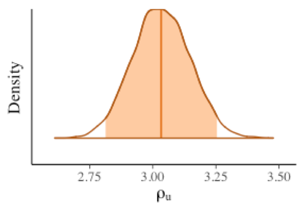
(a) $\rho_{u}$.

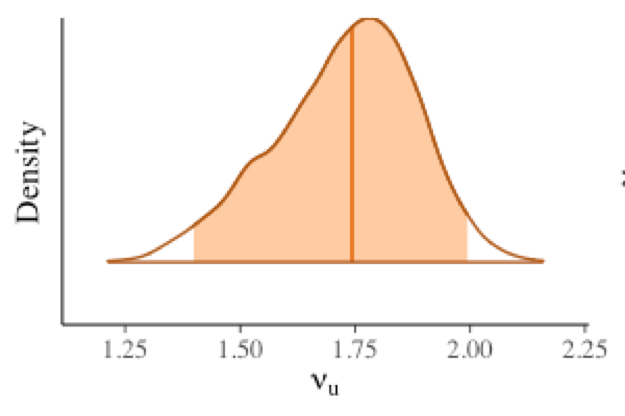
(b) $\nu_{u}$.

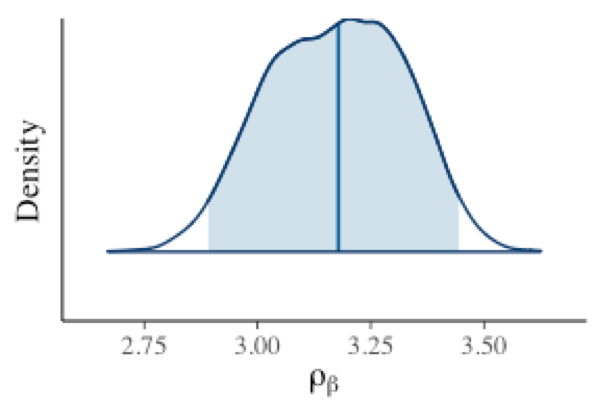
(c) $\rho_{\beta}$.

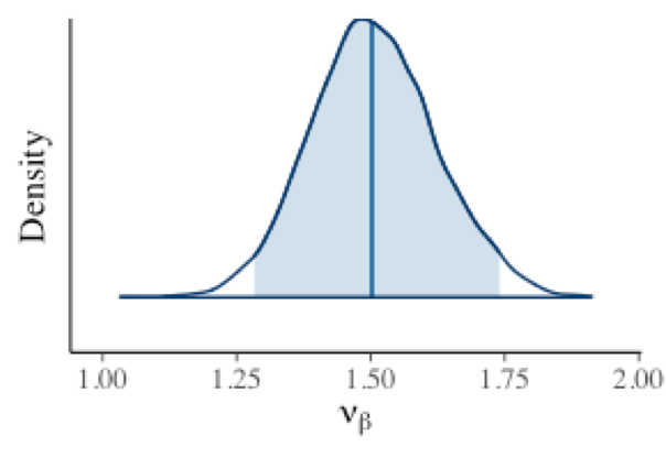
(d) $\nu_{\beta}$.

Figure 3: The posterior densities of spatial parameters for the cocaine user data.

To compare the Bayesian mean estimates to 0 and quantify their uncertainties, the covariate effects on DTs expressed by their posterior z-scores (Louis, 1984) are visualized in Figure 4 and 5, which are smooth over voxels. Among these covariates, cocaine use is the covariate with the most significant impact, where the diagonal coefficients have many absolutely large posterior z-scores located at some regions. Education years has no effect in most areas but a powerful impact at certain areas (see $\beta_{11}$ and $\beta_{31}$), which needs a further scientific investigation. Unlike education years, the effect of age has a significant impact all over the corpus callosum, which may indicate the effect of age on brain structure is little but covers the whole area. Gender and handedness have comparatively small overall effects in comparison to the others but have strong effects in certain areas.

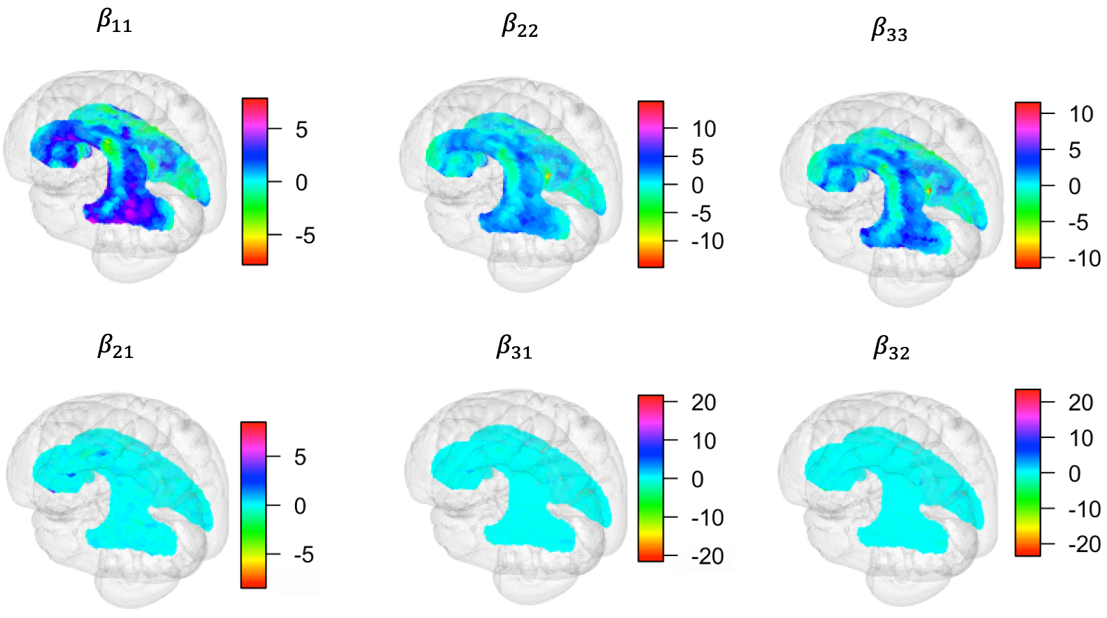
(a) The covariate effects of age.

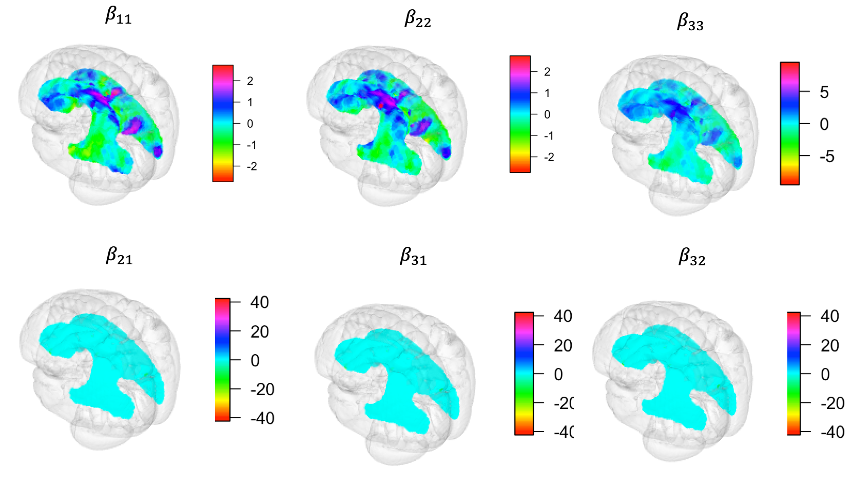
(b) The covariate effects of gender.

Figure 4: The covariate effects of biological attributes on DT expressing by the posterior z-scores of six spatially-varying coefficients.

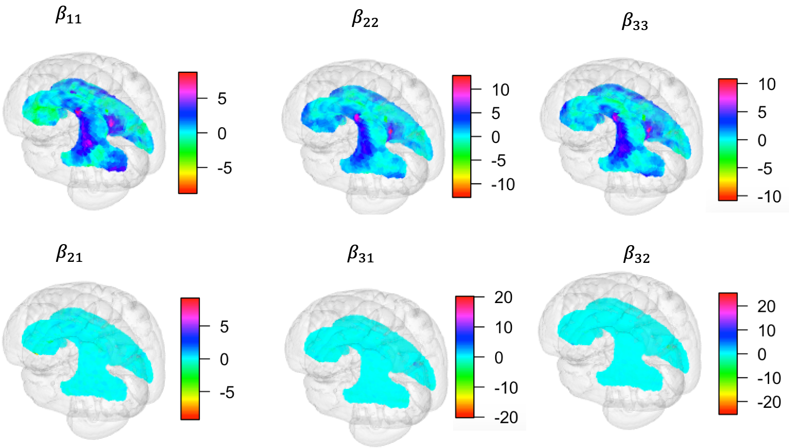
(a) The covariate effects of cocaine use.

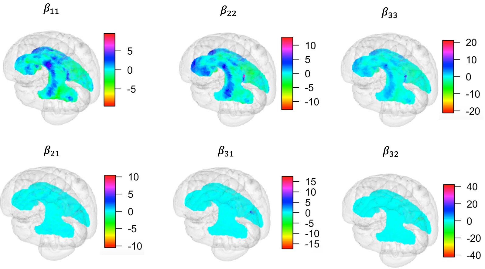
(b) The covariate effects of education years.

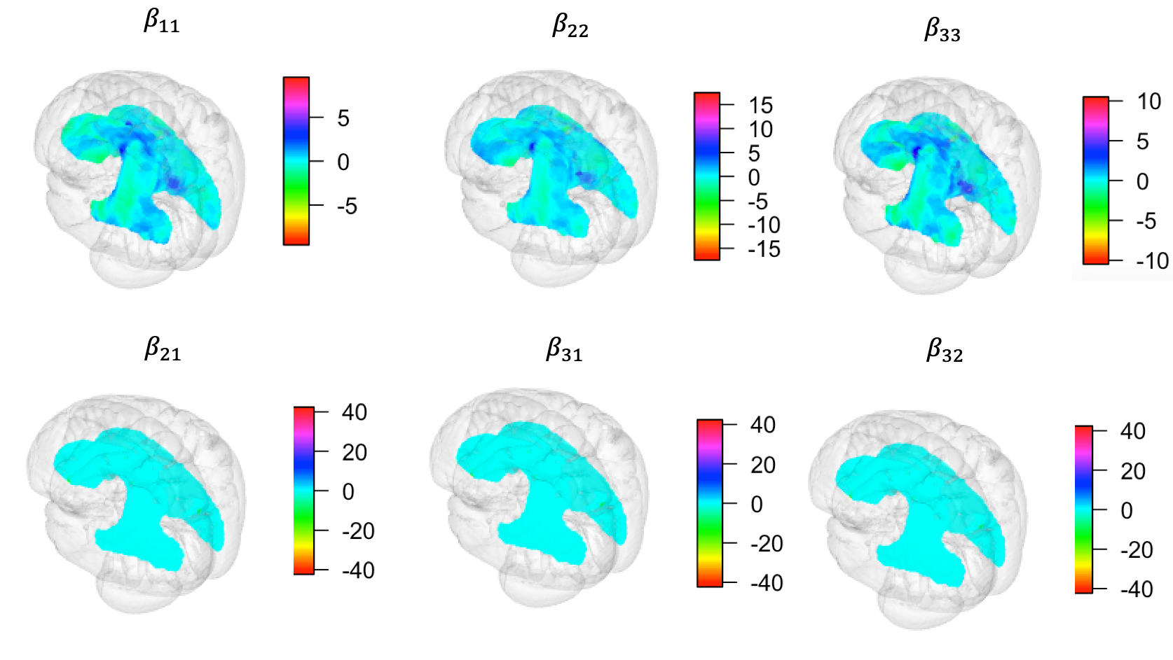
(c) The covariate effects of handedness.

Figure 5: The covariate effects of social attributes on DT expressing by the posterior z-scores of six spatially-varying coefficients.

Furthermore, we use the Markov chain Monte Carlo-based outcome regression estimator to estimate the drug-use effect $\delta_{FA}(\bm{s})$. Figure 6(a) provides the posterior z-scores of $\hat{\delta}_{FA}(\bm{s})$. In comparison, Figure 6(b) provides the posterior z-scores of the Bayesian outcome regression estimator of $\delta_{FA}(\bm{s})$ based on the univariate spatially-varying coefficients model (Gelfand et al., 2003) with the logit transformation of the DTs’ fractional anisotropy as responses. The Cholesky decomposition process model provides a definite region where cocaine use has a significant effect with strong intensity, whereas the effect detected by the univariate model is less distinct. This demonstrates the advantages of the matrix-variate modeling over univariate modeling. The regions of differences are located at the splenium, a component at the posterior end of the corpus callosum, indicating group differences between cocaine users and non-cocaine users. This result is also consistent with previous clinical studies on cocaine use (e.g., Lane et al., 2010), validating the clinical reliability of our proposal.

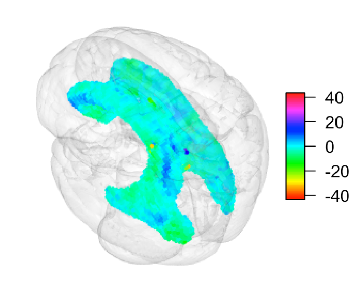
(a) The posterior z-scores of $\delta_{FA}$ based on the Cholesky decomposition process model.

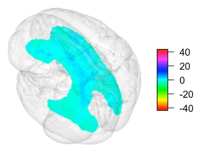
(b) The posterior z-scores of $\delta_{FA}$ based on the univariate model.

Figure 6: The posterior z-scores of $\delta_{FA}$.

6 Discussion

In this paper, we propose geostatistical modeling for positive definite matrices, with applications to DTI. Considering that the literature of spatial modeling of positive definite matrices is sparse, the spatial Wishart process as a random field for spatially dependent positive definite matrices offers a useful and elegant approach. We further propose a Cholesky decomposition process model whose responses are the Cholesky decomposition of positive definite matrices, overcoming the problematic issues caused by the intractable probability density function of the spatial Wishart process. Both the simulation studies and real data application demonstrate the effectiveness in spatial Bayesian inference of positive definite matrices.

Besides neuroimaging application, our work also makes a theoretical contribution to positive definite matrix-variate modeling. A bottleneck of the spatial Wishart process model is that the probability density function is intractable, which here is resolved by proposing the Cholesky decomposition process model. Other attempts are mostly to investigate the special cases where the latent covariance matrix has a certain form (e.g., Mathai and Moschopoulos, 1991; Furman, 2008), compromising the flexibility. Meanwhile, Yu (2004) are proposing characteristic function-based parameter estimation approaches for models whose probability density function is intractable but characteristic function is elegant. In Appendix I, we give the characteristic function of the spatial Wishart process which is simple, providing an alternative inference approach.

The most important contribution is that we have shown that the Cholesky decomposition process model and the spatial Wishart process model are asymptotically equivalent. This might provide an insight that some positive definite matrix-variate models (e.g., Karagiannidis et al., 2003; Smith and Garth, 2007; Kuo et al., 2007) can be approximated to Gaussian processes, allowing statistical and computational benefits brought from Gaussian processes.

Supplementary material

Before showing the proofs, we emphasize again that the Wishart distribution in this paper is a parameterized Wishart distribution in terms of mean matrix and degrees of freedom. That is, let $\bm{A}\sim\mathcal{W}_{p}(\bm{V},n)$, the PDF is

$${\displaystyle f(\mathbf{A})={\frac{\mid\mathbf{A}\mid^{(n-p-1)/2}e^{-\operatorname{tr}([\mathbf{V}/n]^{-1}\mathbf{A})/2}}{2^{\frac{np}{2}}\mid{\mathbf{V}/n}\mid^{n/2}\Gamma_{p}({\frac{n}{2}})}}},$$

with $\mathbb{E}\bm{A}=\bm{V}$. This parameterization is convenient in our model. But this is different from the classic Wishart distribution specified in most classic textbooks of multivariate statistics (i.e., Mardia et al., 1980; Anderson, 1984; Gupta and Nagar, 1999; Eaton et al., 2008), where the mean is $n\bm{V}$. However, there is no difficulty in expressing the results of classic Wishart distribution using this parameterization of the Wishart distribution.

Appendix I

Properties of spatial Wishart process

Before giving the proof, we give the characteristic function of $[\bm{U}(\bm{s}_{1}),...,\bm{U}(\bm{s}_{n})]$ (Corollary 1), making the proof more convenient.

Corollary 1.

The characteristic function of $[\bm{U}(\bm{s}_{1}),...,\bm{U}(\bm{s}_{n})]$ is

$$\phi(\bm{T}_{\bm{s}_{1}},...,\bm{T}_{\bm{s}_{n}})=\mathbb{E}\exp tr[\imath(\bm{T}_{\bm{s}_{1}}\bm{U}(\bm{s}_{1})+...+\bm{T}_{\bm{s}_{n}}\bm{U}(\bm{s}_{n}))]=\mid\bm{I}_{np}-2\imath\bm{T}(\bm{R}\otimes\bm{\Sigma}/m)\mid^{-m/2},$$ (9)

where $\imath$ is the imaginary number with $\imath^{2}=-1$, $\bm{T}_{\bm{s}}$ is a symmetric matrix whose the diagonal entries are $t_{ii}(\bm{s})$ and off-diagonal elements are $\frac{1}{2}t_{ij}(\bm{s})$, $\bm{T}$ is a block diagonal matrix composed of $[\bm{T}_{\bm{s}_{1}},...,\bm{T}_{\bm{s}_{n}}]$, and $\bm{R}$ is the spatial correlation matrix of locations $\{\bm{s}_{1},...,\bm{s}_{n}\}$ constructed by $\mathcal{K}(\bm{s},\bm{s}^{\prime}\mid\bm{\Phi})$.

Proof.

As an extension of Krishnaiah and Rao (1961, Equation 2), the proof largely relies on Anderson (1984, Section 7.3.1), which provides the derivation of characteristic function of a Wishart distribution. We extend Equation (4) of Anderson (1984, Section 7.3.1) to a spatial case:

$$\phi(\bm{T}_{\bm{s}_{1}},...,\bm{T}_{\bm{s}_{n}}) =\prod_{j=1}^{m}\mathbb{E}\exp tr[\imath(\bm{Z}_{j}(\bm{s}_{1})^{T}\bm{T}_{\bm{s}_{1}}\bm{Z}_{j}(\bm{s}_{1})/m+...+\bm{Z}_{j}(\bm{s}_{n})^{T}\bm{T}_{\bm{s}_{n}}\bm{Z}_{j}(\bm{s}_{n})/m)]$$ (10)

$$=(\mathbb{E}\exp tr[\imath(\bm{Z}(\bm{s}_{1})^{T}\bm{T}_{\bm{s}_{1}}\bm{Z}(\bm{s}_{1})/m+...+\bm{Z}(\bm{s}_{n})^{T}\bm{T}_{\bm{s}_{n}}\bm{Z}(\bm{s}_{n})/m)])^{m}$$

$$=(\mathbb{E}\exp tr[\imath\bm{Z}^{T}\bm{T}\bm{Z}/m])^{m}$$

$$=(\mathbb{E}\exp tr[\imath\tilde{\bm{Z}}^{T}\bm{T}\tilde{\bm{Z}}])^{m},$$

where $\tilde{\bm{Z}}$ is a stack vector such as $\tilde{\bm{Z}}=[\bm{Z}(\bm{s}_{1})^{T}/m^{1/2},...,\bm{Z}(\bm{s}_{n})^{T}/m^{1/2}]^{T}$ following a mean-zero Gaussian distribution whose covariance matrix is $\bm{R}\otimes\bm{\Sigma}/m$. Then we can continue to work on the derivation following Anderson (1984, Section 7.3.1) and finally get to Equation (11) of Anderson (1984, Section 7.3.1) under the spatial case. ∎

of Theorem 1.

There are two conditions (K1 and K2) in Kolmogorov’s extension theorem:

K1:

Let $\bm{s}_{1},...,\bm{s}_{K}\in\mathcal{D}$. We want to show for every permutation of observation indices $\pi_{1},...,\pi_{K}$, we have

$$p(\bm{U}(\bm{s}_{1}),...,\bm{U}(\bm{s}_{K}))=p(\bm{U}(\bm{s}_{\pi_{1}}),...,\bm{U}(\bm{s}_{\pi_{K}})).$$

It is equivalent to showing that $\phi(\bm{T}_{\bm{s}_{1}},...,\bm{T}_{\bm{s}_{K}})=\phi(\bm{T}_{\bm{s}_{\pi_{1}}},...,\bm{T}_{\bm{s}_{\pi_{K}}})$; Since the determinant in the characteristic function (9) is invariant to permutation, K1 condition holds.

K2:

The second condition need to verify that, for every location $\bm{s}_{0}\in\mathcal{D}$, we have

$$p(\bm{U}(\bm{s}_{1}),...,\bm{U}(\bm{s}_{K}))=\int p(\bm{U}(\bm{s}_{0}),\bm{U}(\bm{s}_{1}),...,\bm{U}(\bm{s}_{K}))d\bm{U}(\bm{s}_{0}).$$

The characteristic function of $[\bm{U}(\bm{s}_{0}),\bm{U}(\bm{s}_{1}),...,\bm{U}(\bm{s}_{K}))]$ is $\phi(\bm{T}_{\bm{s}_{0}},\bm{T}_{\bm{s}_{1}},...,\bm{T}_{\bm{s}_{K}})$. It is equivalent to showing that $\phi(\bm{T}_{\bm{s}_{0}}=\bm{0},\bm{T}_{\bm{s}_{1}},...,\bm{T}_{\bm{s}_{K}})=\phi(\bm{T}_{\bm{s}_{1}},...,\bm{T}_{\bm{s}_{K}})$, and this follows from the form of the characteristic function (9).

In fact, giving Equation (10) in terms of $\bm{Z}_{j}$ is sufficient to show K1 and K2. Giving Corollary 1 is additional. ∎

of Property 1.

Since Kent (1989) proved that the spatial Gaussian process $\{\bm{Z}_{j}(\bm{s}):\bm{s}\in\mathcal{D}\}$ holds almost-sure continuity under the condition described in the property, we have $\bm{Z}_{j}(\bm{s})\bm{Z}_{j}(\bm{s})^{T}$ converges almost-surely to $\bm{Z}_{j}(\bm{s}_{0})\bm{Z}_{j}(\bm{s}_{0})^{T}$ if $\mid\mid\bm{s}-\bm{s}_{0}\mid\mid\rightarrow 0$ given the continuous mapping theorem (Van der Vaart, 2000, Theorem 2.3). Given the continuous mapping theorem (Van der Vaart, 2000, Theorem 2.3) (we know $[\bm{Z}_{1}(\bm{s})\bm{Z}_{1}(\bm{s})^{T},...,\bm{Z}_{m}(\bm{s})\bm{Z}_{m}(\bm{s})^{T}]^{T}$ converges almost-surely to $[\bm{Z}_{1}(\bm{s}_{0})\bm{Z}_{1}(\bm{s}_{0})^{T},...,\bm{Z}_{m}(\bm{s}_{0})\bm{Z}_{m}(\bm{s}_{0})^{T}]^{T}$ if $\mid\mid\bm{s}-\bm{s}_{0}\mid\mid\rightarrow 0$), we have $\sum_{j}\bm{Z}_{j}(\bm{s})\bm{Z}_{j}(\bm{s})^{T}/m$ converges almost-surely to $\sum_{j}\bm{Z}_{j}(\bm{s}_{0})\bm{Z}_{j}(\bm{s}_{0})^{T}/m$ if $\mid\mid\bm{s}-\bm{s}_{0}\mid\mid\rightarrow 0$, implying that $\{\bm{U}(\bm{s}):\bm{s}\in\mathcal{D}\}$ holds almost-sure continuity. ∎

Appendix II

Preliminary Results

To obtain the asymptotic results, we first establish non-asymptotic results. In particular, we give the marginal distribution (for one location) of spatial Wishart process model by giving Corollary 2 and give the joint distribution (for multiple locations) of spatial Wishart process model by giving Theorem 5.

First, the results of Eaton et al. (2008, Lemma 8.10 and Proposition 8.11) can be summarized as

Theorem 4.

Suppose $\bm{A}\sim\mathcal{W}(\bm{\Sigma},m)$ and $\bm{T}$ is $\bm{A}$’s Cholesky matrix so that $\bm{T}\bm{T}^{T}=\bm{A}$ and $\{t_{kl}\}$ are the elements of $\bm{T}$, then

1. Diagonal: $t_{kk}^{2}\sim\mathcal{GA}(\frac{m-(k-1)}{2},2\sigma_{kk}^{2}/m)$, independent over $k$, where $\sigma_{kk}^{2}$ is the $k$-th diagonal element of $\bm{\Sigma}$;
   

2. Off-Diagonal: if we partition $\bm{A}$, $\bm{T}$ and $\bm{\Sigma}$ as

   $$\bm{A}=\begin{bmatrix}\bm{A}_{11}&\bm{A}_{12}\\ \bm{A}_{21}&\bm{A}_{22}\end{bmatrix},\bm{T}=\begin{bmatrix}\bm{T}_{11}&\bm{0}\\ \bm{T}_{21}&\bm{T}_{22}\end{bmatrix},\bm{\Sigma}=\begin{bmatrix}\bm{\Sigma}_{11}&\bm{\Sigma}_{12}\\ \bm{\Sigma}_{21}&\bm{\Sigma}_{22}\end{bmatrix}$$ (11)

   where $\bm{A}_{kk}$, $\bm{T}_{kk}$, and $\bm{\Sigma}_{kk}$ are $p_{k}\times p_{k}$ square matrices, then

   $$\bm{T}_{21}\mid\bm{T}_{11}\sim\mathcal{MN}_{p_{2},p_{1}}(\bm{T}_{11}\bm{\Sigma}_{11}^{-1}\bm{\Sigma}_{12},[\bm{\Sigma}_{22}-\bm{\Sigma}_{21}\bm{\Sigma}_{11}^{-1}\bm{\Sigma}_{12}]/m,\bm{I}_{p_{1}}).$$

In Theorem 4, $\mathcal{GA}(\alpha,\beta)$ is the gamma distribution with shape parameter $\alpha$ and scale parameter $\beta$; $\mathcal{MN}_{p_{r},p_{c}}(\bm{\mu},\bm{\Sigma}_{r},\bm{\Sigma}_{c})$ is the $p_{r}\times p_{c}$ matrix-variate normal distribution (Dawid, 1981) with mean matrix $\bm{\mu}$, row covariance matrix $\bm{\Sigma}_{r}$ and column covariance matrix $\bm{\Sigma}_{c}$. To apply this result to the spatial Wishart process, let $\bm{T}_{i}(\bm{s})$ be the Cholesky decomposition of $\bm{A}_{i}(\bm{s})$ with $\bm{A}_{i}(\bm{s})=\bm{T}_{i}(\bm{s})\bm{T}_{i}(\bm{s})^{T}$ and $t_{ikl}(\bm{s})$ be the $(k,l)$-th element of $\bm{T}_{i}(\bm{s})$. Since $\bm{A}_{i}(\bm{s})$ can also be decomposed as $\bm{L}_{i}(\bm{s})\bm{U}_{i}(\bm{s})\bm{L}_{i}(\bm{s})^{T}$, we give Corollary 2:

Corollary 2.

Suppose $\bm{A}\sim\mathcal{W}(\bm{\Sigma},m)$ has the Cholesky decomposition $\bm{T}\bm{T}^{T}=\bm{A}$. Also $\bm{A}=\bm{L}\bm{U}\bm{L}^{T}$ where $\bm{L}\bm{L}^{T}=\bm{\Sigma}$ and $\bm{U}\sim\mathcal{W}(\bm{I},m)$ with Cholesky decomposition $\bm{D}\bm{D}^{T}=\bm{U}$. If $\{t_{kl}\}$ and $\{d_{kl}\}$ are the Cholesky decomposition elements of $\bm{A}$ and $\bm{U}$, respectively, then

1. Diagonal: $t_{kk}^{2}=d_{kk}^{2}l_{kk}^{2}\sim\mathcal{GA}(\frac{m-(k-1)}{2},2l_{kk}^{2}/m)$, where $l_{kk}$ is the $k$-th diagonal element of $\bm{L}$;
   

2. Off-Diagonal: if we partition $\bm{L}$, $\bm{T}$, and $\bm{D}$ as

   $$\bm{L}=\begin{bmatrix}\bm{L}_{11}&\bm{0}\\ \bm{L}_{21}&\bm{L}_{22}\end{bmatrix},\bm{T}=\begin{bmatrix}\bm{T}_{11}&\bm{0}\\ \bm{T}_{21}&\bm{T}_{22}\end{bmatrix},\bm{D}=\begin{bmatrix}\bm{D}_{11}&\bm{0}\\ \bm{D}_{21}&\bm{D}_{22}\end{bmatrix}$$ (12)

   where $\bm{L}_{kk}$, $\bm{T}_{kk}$, $\bm{D}_{kk}$ are $p_{k}\times p_{k}$ square matrices, then

   $$\bm{T}_{21}\mid\bm{T}_{11}\sim\mathcal{MN}_{p_{2},p_{1}}(\bm{L}_{21}\bm{D}_{11},\bm{L}_{22}\bm{L}_{22}^{T}/m,\bm{I}_{p_{1}}).$$

Proof.

1. Diagonal: It is easy to show $t_{kk}^{2}=d_{kk}^{2}l_{kk}^{2}$ and $d_{kk}^{2}\sim\mathcal{GA}(\frac{m-(k-1)}{2},2/m)$, hence $t_{kk}^{2}=d_{kk}^{2}l_{kk}^{2}\sim\mathcal{GA}(\frac{m-(k-1)}{2},2l_{kk}^{2}/m)$;
   

2. Off-Diagonal: From Theorem 4 and Gupta and Nagar (1999, Theorem 2.3.1), we have $\bm{D}_{21}\mid\bm{D}_{11}\sim\mathcal{MN}_{p_{2},p_{1}}(\bm{D}_{11},\bm{I}_{p_{2}},\bm{I}_{p_{1}})$. We know

   $$\begin{bmatrix}\bm{T}_{11}&\bm{0}\\ \bm{T}_{21}&\bm{T}_{22}\end{bmatrix}=\begin{bmatrix}\bm{L}_{11}&\bm{0}\\ \bm{L}_{21}&\bm{L}_{22}\end{bmatrix}\begin{bmatrix}\bm{D}_{11}&\bm{0}\\ \bm{D}_{21}&\bm{D}_{22}\end{bmatrix}=\begin{bmatrix}\bm{L}_{11}\bm{D}_{11}&\bm{0}\\ \bm{L}_{21}\bm{D}_{11}+\bm{L}_{22}\bm{D}_{21}&\bm{L}_{22}\bm{D}_{22}\end{bmatrix}$$ (13)

   Given Gupta and Nagar (1999, Theorem 2.3.10), we have

   $$\bm{T}_{21}\mid\bm{T}_{11}\sim\mathcal{MN}_{p_{2},p_{1}}(\bm{L}_{21}\bm{D}_{11},\bm{L}_{22}\bm{L}_{22}^{T}/m,\bm{I}_{p_{1}}).$$

Now, we have proven all the statements. ∎

By Corollary 2, the diagonal elements $t^{2}_{ikk}(\bm{s})$ marginally follow gamma distributions

$$e^{2}_{ikk}(\bm{s})\sim\mathcal{GA}\left(\frac{m-(k-1)}{2},\frac{2e^{2\bm{X}_{i}\bm{\beta}_{kk}(\bm{s})}}{m}\right).$$ (14)

The marginal distributions of off-diagonal elements are

$$e_{{i21}}(\bm{s})\mid d_{{i11}}(\bm{s}) \sim\mathcal{N}(d_{{i11}}(\bm{s})\bm{X}_{i}\bm{\beta}_{21}(\bm{s}),e^{2\bm{X}_{i}\bm{\beta}_{22}(\bm{s})}/m)$$ (15)

$$e_{{i31}}(\bm{s})\mid d_{{i11}}(\bm{s}),d_{{i21}}(\bm{s}) \sim\mathcal{N}(d_{{i11}}(\bm{s})\bm{X}_{i}\bm{\beta}_{31}(\bm{s})+d_{i21}(\bm{s})\bm{X}_{i}\bm{\beta}_{32}(\bm{s}),e^{2\bm{X}_{i}\bm{\beta}_{33}(\bm{s})}/m)$$

$$t_{{i32}}(\bm{s})\mid d_{{i22}}(\bm{s}) \sim\mathcal{N}(d_{{i22}}(\bm{s})\bm{X}_{i}\bm{\beta}_{32}(\bm{s}),e^{2\bm{X}_{i}\bm{\beta}_{33}(\bm{s})}/m),$$

where $\bm{Z}_{ij}(\bm{s})=[Z_{ij1}(\bm{s}),Z_{ij2}(\bm{s}),Z_{ij3}(\bm{s})]^{T}$, $\bm{Z}_{ij}\sim\mathcal{GP}(\bm{0},\mathcal{K}(\bm{s},\bm{s}^{\prime}\mid\bm{\Phi}_{u}),\bm{I})$ (the term is independent distributed over $j$ here, and $i$ is a given and fixed subject index), and $d_{ikl}(\bm{s})$ is the (k,l)-th Cholesky decomposition elements of $\sum_{j=1}^{m}\bm{Z}_{ij}(\bm{s})\bm{Z}_{ij}(\bm{s})^{T}/m$.

Now we give Theorem 5:

Theorem 5.

If $\bm{U}\sim\mathcal{SWP}(m,\mathcal{K}(\bm{s},\bm{s}^{\prime}\mid\bm{\Phi}),\bm{I})$, $\bm{Z}_{j}=[\bm{Z}_{j1}^{T},\bm{Z}_{j2}^{T}]^{T}\sim\mathcal{GP}(\bm{0},\mathcal{K}(\bm{s},\bm{s}^{\prime}\mid\bm{\Phi}),\bm{I})$, and $\{d_{{kl}}(\bm{s})\}$ are elements of $\bm{U}(\bm{s})$’s Cholesky decomposition with $\bm{D}(\bm{s})\bm{D}(\bm{s})^{T}=\bm{U}(\bm{s})$, then

1. Diagonal: $d_{kk}^{2}\sim\mathcal{SWP}(m-(k-1),\mathcal{K}(\bm{s},\bm{s}^{\prime}\mid\bm{\Phi}),1)$;
   

2. Off-diagonal: If we partition $\bm{U}(\bm{s})$ and $\bm{D}(\bm{s})$ as $\bm{U}(\bm{s})=\begin{bmatrix}\bm{U}_{11}(\bm{s})&\bm{U}_{12}(\bm{s})\\ \bm{U}_{21}(\bm{s})&\bm{U}_{22}(\bm{s})\end{bmatrix}$, $\bm{D}(\bm{s})=\begin{bmatrix}\bm{D}_{11}(\bm{s})&\bm{0}\\ \bm{D}_{21}(\bm{s})&\bm{D}_{22}(\bm{s})\end{bmatrix}$, respectively, where $\bm{U}_{kk}(\bm{s})$ and $\bm{D}_{kk}(\bm{s})$ are $p_{k}\times p_{k}$ square matrices with $\bm{U}_{11}(\bm{s})=\frac{1}{m}\sum_{j=1}^{m}\bm{Z}_{j1}(\bm{s})\bm{Z}_{j1}(\bm{s})^{T}$, then conditional on $\mathbf{S}_{\bm{D}_{21}}=\{\bm{Z}_{j1}(\bm{s}):j=\{1,2,...,m\},\bm{s}\in\mathcal{D}\}$, the term $\{vect[\bm{D}_{21}(\bm{s})]:\bm{s}\in\mathcal{D}\}$ is a mean-zero multivariate Gaussian process with spatial covariance ${cov}(vect[\bm{D}_{21}(\bm{s})],vect[\bm{D}_{21}(\bm{s}^{\prime})]\mid\mathbf{S}_{\bm{D}_{21}})=\mathcal{K}(\bm{s},\bm{s}^{\prime}\mid\bm{\Phi})\bm{I}_{p_{2}}\otimes\frac{1}{m}\bm{D}_{11}(\bm{s})^{-1}\left[\sum_{j=1}^{m}\bm{Z}_{j1}(\bm{s})\bm{Z}_{j1}(\bm{s}^{\prime})^{T}/m\right][\bm{D}_{11}(\bm{s}^{\prime})^{-1}]^{T}$. $vect$ is a notation for matrix vectorization.

Proof.

1. Diagonal: Mardia et al. (1980, Theorem 3.4.4) have given the relevant proofs for the non-spatial case and it is not difficult to extend it to the spatial case. Eaton et al. (2008, Section 8.2) give that $m\bm{U}_{22.1}(\bm{s})=m\bm{D}_{22}(\bm{s})\bm{D}_{22}(\bm{s})^{T}=\bm{X}_{2}(\bm{s})^{T}\bm{X}_{2}(\bm{s})-\bm{X}_{2}(\bm{s})^{T}\bm{X}_{1}(\bm{s})(\bm{X}_{1}(\bm{s})^{T}\bm{X}_{1}(\bm{s}))^{-1}\bm{X}_{1}(\bm{s})^{T}\bm{X}_{2}(\bm{s})=\bm{X}_{2}(\bm{s})^{T}\bm{Q}(\bm{s})\bm{X}_{2}(\bm{s})$. In Mardia et al. (1980), the term $\bm{X}_{q}(\bm{s})=[\bm{Z}_{1q}(\bm{s}),...,\bm{Z}_{mq}(\bm{s})]^{T}$ is called normal data matrix of $\mathcal{N}(\bm{0},\bm{I}_{p_{q}})$ (marginally). The term $\bm{Q}(\bm{s})$ is an idempotent matrix with rank $m-p_{1}$. We do spectral decomposition of $\bm{Q}(\bm{s})$ to have $\bm{Q}(\bm{s})=\bm{\Gamma}(\bm{s})^{T}\bm{\Lambda}\bm{\Gamma}(\bm{s})$ and the property of idempotent matrix gives that $\bm{\Lambda}$ is a diagonal matrix with $m-p_{1}$ non-zero eigenvalues which equal to 1. The proof of Mardia et al. (1980, Theorem 3.4.4) shows that $\bm{Y}(\bm{s})=\bm{\Gamma}(\bm{s})\bm{X}_{2}(\bm{s})$ is a normal data matrix of $\mathcal{N}(\bm{0},\bm{I}_{p_{2}})$ given Mardia et al. (1980, Theorem 3.3.2). We have $cor(\bm{Y}(\bm{s}),\bm{Y}(\bm{s}^{\prime})\mid\bm{\Gamma}(\bm{s}))=\mathcal{K}(\bm{s},\bm{s}^{\prime})=cor(\bm{Y}(\bm{s}),\bm{Y}(\bm{s}^{\prime}))$. Then we finally have $\bm{D}_{22}(\bm{s})\bm{D}_{22}(\bm{s})^{T}=\frac{1}{m}\sum_{j=1}^{m-p_{1}}\bm{Y}_{j}(\bm{s})\bm{Y}_{j}(\bm{s})^{T}$ and $\bm{Y}_{j}\sim\mathcal{GP}(0,\mathcal{K}(\bm{s},\bm{s}^{\prime}\mid\bm{\Phi}),\bm{I})$. Therefore, we prove the first statement.
   

2. Off-Diagonal: We show the result using moment generating function. For a concise illustration, we give $p_{1}=p_{2}=1$.

   $$M(t_{\bm{s}_{1}},...t_{\bm{s}_{n}})$$ (16)

   $$=\mathbb{E}[\exp(t_{\bm{s}}d_{21}(\bm{s}_{1})+...+t_{\bm{s}^{\prime}}d_{21}(\bm{s}_{n}))\mid Z_{j1},j=\{1,2,...,m\}]$$

   $$=\mathbb{E}[t_{\bm{s}}\frac{1}{m}\sum_{j=1}^{m}Z_{j2}(\bm{s})Z_{j1}(\bm{s})/d_{11}(\bm{s})+t_{\bm{s}^{\prime}}\frac{1}{m}\sum_{j=1}^{m}Z_{j2}(\bm{s}^{\prime})Z_{j1}(\bm{s}^{\prime})/d_{11}(\bm{s}^{\prime})\mid Z_{j1},j=\{1,2,...,m\}]$$

   because $$\frac{1}{m}\sum_{j=1}^{m}Z_{j2}(\bm{s})Z_{j1}(\bm{s})=U_{21}(\bm{s})=d_{21}(\bm{s})d_{11}(\bm{s})$$), see the proof of Eaton et al. (2008, Lemma 8.10)

   $$=\exp([t_{\bm{s}_{1}},...,t_{\bm{s}_{n}}]^{T}\bm{Q}[t_{\bm{s}_{1}},...,t_{\bm{s}_{n}}])$$

   (because $$Z_{j2}\sim\mathcal{GP}(0,\mathcal{K}(\bm{s},\bm{s}^{\prime}\mid\bm{\Phi}),1)$$)

   $\bm{Q}$ is a symmetric matrix with diagonal elements are $\frac{1}{m^{2}}\sum_{j=1}^{m}Z_{j1}(\bm{s})^{2}$ for $\bm{s}\in\mathcal{D}$ and off-diagonal elements $\frac{1}{m^{2}}\sum_{j=1}^{m}Z_{j1}(\bm{s})Z_{j1}(\bm{s}^{\prime})\mathcal{K}(\bm{s},\bm{s}^{\prime}\mid\bm{\Phi})$ for all $\bm{s}\not=\bm{s}^{\prime}$.

   Then we conclude that the off-diagonal elements $d_{21}$ are conditionally normal distributed. It is not difficult to extend this result to multivariate/matrix-variate cases. Here, we just need to derive the covariance. Following the result that $\frac{1}{m}\sum_{j=1}^{m}\bm{Z}_{j2}(\bm{s})\bm{Z}_{j1}(\bm{s})^{T}=\bm{U}_{21}(\bm{s})=\bm{D}_{21}(\bm{s})\bm{D}_{11}(\bm{s})^{T}$, we have

   $$cov(vect[\bm{D}_{21}(\bm{s})],vect[\bm{D}_{21}(\bm{s}^{\prime})]\mid\bm{S}_{\bm{D}_{21}})$$ (17)

   $$=\mathcal{K}(\bm{s},\bm{s}^{\prime}\mid\bm{\Phi})\bm{I}_{p_{2}}\otimes\frac{1}{m}\bm{D}_{11}(\bm{s})^{-1}\left[\sum_{j=1}^{m}\bm{Z}_{j1}(\bm{s})\bm{Z}_{j1}(\bm{s}^{\prime})^{T}/m\right][\bm{D}_{11}(\bm{s}^{\prime})^{-1}]^{T}$$

Now, we have proven all the statements. ∎

Given Theorem 5, we have that the diagonal element $e^{2}_{ikk}$ follow a spatial Wishart process, denoted as

$$e_{ikk}^{2}\sim\mathcal{SWP}(m-(k-1),\mathcal{K}(\bm{s},\bm{s}^{\prime}\mid\bm{\Phi}_{u})e^{\sum_{\bm{\omega}\in\{\bm{s},\bm{s}^{\prime}\}}2\bm{X}_{i}\bm{\beta}_{kk}(\bm{\omega})},1).$$ (18)

In addition, the off-diagonal element $e_{ikl}$ conditionally follow a univariate spatial Gaussian process, denoted as

$$e_{{i21}}\mid\bm{S}_{e_{i21}}\sim\mathcal{GP}(d_{i11}(\bm{s})\bm{X}_{i}\bm{\beta}_{21}(\bm{s}),\mathcal{K}(\bm{s},\bm{s}^{\prime}\mid\bm{\Phi}_{u})Q_{ij1}\ e^{\sum_{\bm{w}\in\{\bm{s},\bm{s}^{\prime}\}}\bm{X}_{i}\bm{\beta}_{22}(\bm{w})},\frac{1}{m})$$ (19)

$$e_{{i31}}\mid\bm{S}_{e_{i31}}\sim\mathcal{GP}(d_{i11}(\bm{s})\bm{X}_{i}\bm{\beta}_{31}(\bm{s})+d_{{i21}}(\bm{s})\bm{X}_{i}\bm{\beta}_{32}(\bm{s}),\mathcal{K}(\bm{s},\bm{s}^{\prime}\mid\bm{\Phi}_{u})Q_{ij1}\ e^{\sum_{\bm{w}\in\{\bm{s},\bm{s}^{\prime}\}}\bm{X}_{i}\bm{\beta}_{33}(\bm{w})},\frac{1}{m})$$

$$e_{{i32}}\mid\bm{S}_{e_{i32}}\sim\mathcal{GP}(d_{i22}(\bm{s})\bm{X}_{i}\bm{\beta}_{32}(\bm{s}),\mathcal{K}(\bm{s},\bm{s}^{\prime}\mid\bm{\Phi}_{u})Q_{ij2}\ e^{\sum_{\bm{w}\in\{\bm{s},\bm{s}^{\prime}\}}\bm{X}_{i}\bm{\beta}_{33}(\bm{w})},\frac{1}{m}),$$

where $Q_{ijl}=\frac{\sum_{j=1}^{m}Z_{ijl}(\bm{s})Z_{ijl}(\bm{s}^{\prime})/m}{d_{ill}(\bm{s})d_{ill}(\bm{s}^{\prime})}$. Note that the conditional component $\bm{S}_{e_{ikl}}$ is invariant to the terms on the right-hand side.

Proofs of Asymptotic Results

of Theorem 3.

The spatial joint distribution of diagonal elements $e_{ikk}(\bm{s})$ is a multivariate Gamma distribution defined in Krishnaiah and Rao (1961). Krishnaiah and Rao (1961, Lemma 1) also show that the correlation matrix of the Gamma random variables is a matrix defined by $\mathcal{C}(\bm{s},\bm{s}^{\prime}\mid\bm{\Phi}_{u})=\mathcal{K}(\bm{s},\bm{s}^{\prime}\mid\bm{\Phi}_{u})^{2}$. Since Gamma distribution can be considered as a summation of independent squared Gaussian distributed variables ($m$ is an integer), it is not difficult to have that as $m\rightarrow\infty$, we have the result of convergence in distribution:

$$m^{1/2}[e_{ikk}^{2}(\bm{s}_{1})-e^{2\bm{X}_{i}\bm{\beta}_{kk}(\bm{s}_{1})},...,e_{ikk}^{2}(\bm{s}_{n})-e^{2\bm{X}_{i}\bm{\beta}_{kk}(\bm{s}_{n}})]^{T}\rightarrow\mathcal{GP}(0,\mathcal{C}(\bm{s},\bm{s}^{\prime}\mid\bm{\Phi}_{u})e^{\sum_{\bm{\omega}\in\{\bm{s},\bm{s}^{\prime}\}}2\bm{X}_{i}\bm{\beta}_{kk}(\bm{\omega})},2),$$

given the central limit theorem and Slutsky’s theorem. Taking the logarithm on the diagonal elements and applying the delta method, the term $e^{\sum_{\bm{\omega}\in\{\bm{s},\bm{s}^{\prime}\}}2\bm{X}_{i}\bm{\beta}_{kk}(\bm{\omega})}$ is cancelled. We show the detailed steps below:

Let $g(X_{1},...,X_{n})=[\frac{1}{2}\log X_{1},...,\frac{1}{2}\log X_{n}]^{T}$. We have $\nabla g(X_{1},...,X_{n})=\frac{1}{2}diag[\frac{1}{X_{1}},...,\frac{1}{X_{n}}]$. We know the covariance matrix of $m^{1/2}[e_{ikk}^{2}(\bm{s}_{1})-e^{2\bm{X}_{i}\bm{\beta}_{kk}(\bm{s}_{1})},...,e_{ikk}^{2}(\bm{s}_{n})-e^{2\bm{X}_{i}\bm{\beta}_{kk}(\bm{s}_{n}})]^{T}$ is $\bm{O}=2\times diag(e^{2\bm{X}_{i}\bm{\beta}_{kk}(\bm{s}_{1})},...,e^{2\bm{X}_{i}\bm{\beta}_{kk}(\bm{s}_{n})})\bm{R}_{c}diag(e^{2\bm{X}_{i}\bm{\beta}_{kk}(\bm{s}_{1})},...,e^{2\bm{X}_{i}\bm{\beta}_{kk}(\bm{s}_{n})})$, where $\bm{R}_{c}$ is the correlation matrix constructed by $\mathcal{C}(\bm{s},\bm{s}^{\prime}|\bm{\Phi}_{u})$. Following delta method, we have that the covariance matrix of $m^{1/2}[\log e_{ikk}(\bm{s}_{1})-\bm{X}_{i}\bm{\beta}_{kk}(\bm{s}_{1}),...,\log e_{ikk}(\bm{s}_{n})-\bm{X}_{i}\bm{\beta}_{kk}(\bm{s}_{n})]^{T}$ is $\mathbf{K}=\nabla g(X_{1},...,X_{n})^{T}\mathbf{O}\nabla g(X_{1},...,X_{n})=\frac{1}{2}\mathbf{R}_{c}$. Hence, we have the result of convergence in distribution:

$$m^{1/2}[\log e_{ikk}(\bm{s}_{1})-\bm{X}_{i}\bm{\beta}_{kk}(\bm{s}_{1}),...,\log e_{ikk}(\bm{s}_{n})-\bm{X}_{i}\bm{\beta}_{kk}(\bm{s}_{n})]^{T}\rightarrow\mathcal{GP}\left(0,\mathcal{C}(\bm{s},\bm{s}^{\prime}\mid\bm{\Phi}_{u}),{\frac{1}{2}}\right).$$

Therefore, we have proven the first statement. Please note here we abuse the notation $\mathcal{GP}$ because this notation is originally created for a process. However, since it does not cause any problems when used for a distribution, we simply continue to use $\mathcal{GP}$ without introducing any additional notations.

We note that as $m\rightarrow\infty$, $d_{ikk}(\bm{s})$ converges in probability to $1$, $d_{ikl}(\bm{s})$ converges in probability to $0$, and $Q_{ijl}$ converges in probability to $\mathcal{K}(\bm{s},\bm{s}^{\prime}\mid\bm{\Phi}_{u})$, given law of large numbers and continuous mapping theorem (Van der Vaart, 2000, Theorem 2.3). We have $\mathbb{E}[[e_{{ikl}}(\bm{s}_{1}),...,e_{{ikl}}(\bm{s}_{n})]^{T}\mid\bm{S}_{e_{ikl}}]$ converges in probability to $\mathbb{E}[[t_{{ikl}}(\bm{s}_{1}),...,t_{{ikl}}(\bm{s}_{n})]^{T}\mid\bar{t}_{ikk}]$, $cor(e_{{ikl}}(\bm{s}),e_{{ikl}}(\bm{s}^{\prime})\mid\bm{S}_{e_{ikl}})$ converges in probability to $\mathcal{K}(\bm{s},\bm{s}^{\prime}\mid\bm{\Phi})^{2}=\mathcal{C}(\bm{s},\bm{s}^{\prime}\mid\bm{\Phi})$.

Given the Slutsky’s theorem and $\bm{\beta}_{kl}(\bm{s})=\bm{0}$, we have the following results about convergence in distribution:

$$m^{1/2}e_{{i21}}\mid\bm{S}_{e_{i21}}\rightarrow\mathcal{GP}(0,\mathcal{C}(\bm{s},\bm{s}^{\prime}\mid\bm{\Phi}_{u})e^{\sum_{\bm{w}\in\{\bm{s},\bm{s}^{\prime}\}}\bm{X}_{i}\bm{\beta}_{22}(\bm{w})},1)$$ (20)

$$m^{1/2}e_{{i31}}\mid\bm{S}_{e_{i31}}\rightarrow\mathcal{GP}(0,\mathcal{C}(\bm{s},\bm{s}^{\prime}\mid\bm{\Phi}_{u})e^{\sum_{\bm{w}\in\{\bm{s},\bm{s}^{\prime}\}}\bm{X}_{i}\bm{\beta}_{33}(\bm{w})},1)$$

$$m^{1/2}e_{{i32}}\mid\bm{S}_{e_{i32}}\rightarrow\mathcal{GP}(0,\mathcal{C}(\bm{s},\bm{s}^{\prime}\mid\bm{\Phi}_{u})e^{\sum_{\bm{w}\in\{\bm{s},\bm{s}^{\prime}\}}\bm{X}_{i}\bm{\beta}_{33}(\bm{w})},1),$$

Also, we have $\bar{t}_{ikk}(\bm{s})$ converges in probability $e^{\bm{X}_{i}\bm{\beta}_{kk}(\bm{s})}$ as $N\rightarrow\infty$, given law of large number and continuous mapping theorem (Van der Vaart, 2000, Theorem 2.3). Given the Slutsky’s theorem and $\bm{\beta}_{kl}(\bm{s})=\bm{0}$, we have the following results about convergence in distribution:

$$m^{1/2}t_{{i21}}\mid\bar{t}_{{i22}}\rightarrow\mathcal{GP}(0,\mathcal{C}(\bm{s},\bm{s}^{\prime}\mid\bm{\Phi}_{u})e^{\sum_{\bm{w}\in\{\bm{s},\bm{s}^{\prime}\}}\bm{X}_{i}\bm{\beta}_{22}(\bm{w})},1)$$ (21)

$$m^{1/2}t_{{i31}}\mid\bar{t}_{{i33}}\rightarrow\mathcal{GP}(0,\mathcal{C}(\bm{s},\bm{s}^{\prime}\mid\bm{\Phi}_{u})e^{\sum_{\bm{w}\in\{\bm{s},\bm{s}^{\prime}\}}\bm{X}_{i}\bm{\beta}_{33}(\bm{w})},1)$$

$$m^{1/2}t_{{i32}}\mid\bar{t}_{{i33}}\rightarrow\mathcal{GP}(0,\mathcal{C}(\bm{s},\bm{s}^{\prime}\mid\bm{\Phi}_{u})e^{\sum_{\bm{w}\in\{\bm{s},\bm{s}^{\prime}\}}\bm{X}_{i}\bm{\beta}_{33}(\bm{w})},1).$$

Now, we have proven the second statement because both converge to the same distribution/process. ∎

Cholesky Decomposition Process

of Theorem 2.

Since the measures on the Cholesky decomposition process model and the spatial Wishart process model can be one-to-one mutually transformed. It is not difficult to obtain the results based on the proofs in Appendix I. In addition, given the continuous mapping theorem (Van der Vaart, 2000, Theorem 2.3), we have the almost-sure continuity. ∎

References

• Anderson (1984) Anderson, T. W. (1984). An introduction to multivariate statistical analysis. Technical report, Wiley New York.
• Blumenson and Miller (1963) Blumenson, L. and Miller, K. (1963). Properties of generalized rayleigh distributions. The Annals of Mathematical Statistics 34, 903–910.
• Brick and Erickson (1998) Brick, J. and Erickson, C. K. (1998). Drugs, the brain, and behavior: The pharmacology of abuse and dependence. Haworth Medical Press.
• Cressie (1992) Cressie, N. (1992). Statistics for spatial data. Terra Nova 4, 613–617.
• Datta et al. (2016) Datta, A., Banerjee, S., Finley, A. O., and Gelfand, A. E. (2016). Hierarchical nearest-neighbor gaussian process models for large geostatistical datasets. Journal of the American Statistical Association 111, 800–812.
• Dawid (1981) Dawid, A. P. (1981). Some matrix-variate distribution theory: notational considerations and a Bayesian application. Biometrika 68, 265–274.
• Dryden et al. (2009) Dryden, I. L., Koloydenko, A., and Zhou, D. (2009). Non-Euclidean statistics for covariance matrices, with applications to diffusion tensor imaging. The Annals of Applied Statistics pages 1102–1123.
• Eaton et al. (2008) Eaton, M., Euclid, P., Library, C. U., and Press, D. U. (2008). Multivariate Statistics: A Vector Space Approach. Lecture notes-monograph series. Cornell University Library.
• Ennis and Kindlmann (2006) Ennis, D. B. and Kindlmann, G. (2006). Orthogonal tensor invariants and the analysis of diffusion tensor magnetic resonance images. Magnetic Resonance in Medicine: An Official Journal of the International Society for Magnetic Resonance in Medicine 55, 136–146.
• Furman (2008) Furman, E. (2008). On a multivariate gamma distribution. Statistics & Probability Letters 78, 2353–2360.
• Gelfand et al. (2010) Gelfand, A. E., Fuentes, M., Guttorp, P., and Diggle, P. (2010). Continuous parameter stochastic process theory. In Handbook of Spatial Statistics, pages 25–36. CRC Press.
• Gelfand et al. (2003) Gelfand, A. E., Kim, H.-J., Sirmans, C., and Banerjee, S. (2003). Spatial modeling with spatially varying coefficient processes. Journal of the American Statistical Association 98, 387–396.
• Gelfand et al. (2004) Gelfand, A. E., Schmidt, A. M., Banerjee, S., and Sirmans, C. (2004). Nonstationary multivariate process modeling through spatially varying coregionalization. Test 13, 263–312.
• Gupta and Nagar (1999) Gupta, A. K. and Nagar, D. K. (1999). Matrix variate distributions, volume 104. CRC Press.
• Heaton et al. (2018) Heaton, M. J., Datta, A., Finley, A. O., Furrer, R., Guinness, J., Guhaniyogi, R., Gerber, F., Gramacy, R. B., Hammerling, D., Katzfuss, M., et al. (2018). A case study competition among methods for analyzing large spatial data. Journal of Agricultural, Biological and Environmental Statistics pages 1–28.
• Karagiannidis et al. (2003) Karagiannidis, G. K., Zogas, D. A., and Kotsopoulos, S. A. (2003). An efficient approach to multivariate nakagami-m distribution using green’s matrix approximation. IEEE Transactions on Wireless Communications 2, 883–889.
• Kent (1989) Kent, J. T. (1989). Continuity properties for random fields. The Annals of Probability pages 1432–1440.
• Krishnaiah and Rao (1961) Krishnaiah, P. and Rao, M. (1961). Remarks on a multivariate gamma distribution. American Mathematical Monthly pages 342–346.
• Kuo et al. (2007) Kuo, P.-H., Smith, P. J., and Garth, L. M. (2007). Joint density for eigenvalues of two correlated complex wishart matrices: Characterization of mimo systems. IEEE Transactions on Wireless Communications 6, 3902–3906.
• Lan et al. (2019) Lan, Z., Reich, B. J., and Bandyopadhyay, D. (2019). A spatial bayesian semiparametric mixture model for positive definite matrices with applications to diffusion tensor imaging. arXiv preprint arXiv:1903.07509 .
• Lane et al. (2010) Lane, S. D., Steinberg, J. L., Ma, L., Hasan, K. M., Kramer, L. A., Zuniga, E. A., Narayana, P. A., and Moeller, F. G. (2010). Diffusion tensor imaging and decision making in cocaine dependence. PLoS One 5, e11591.
• Leone et al. (1961) Leone, F., Nelson, L., and Nottingham, R. (1961). The folded normal distribution. Technometrics 3, 543–550.
• Lo et al. (2010) Lo, C.-Y., Wang, P.-N., Chou, K.-H., Wang, J., He, Y., and Lin, C.-P. (2010). Diffusion tensor tractography reveals abnormal topological organization in structural cortical networks in Alzheimer’s disease. Journal of Neuroscience 30, 16876–16885.
• Louis (1984) Louis, T. A. (1984). Estimating a population of parameter values using bayes and empirical bayes methods. Journal of the American Statistical Association 79, 393–398.
• Ma et al. (2017) Ma, L., Steinberg, J. L., Wang, Q., Schmitz, J. M., Boone, E. L., Narayana, P. A., and Moeller, F. G. (2017). A preliminary longitudinal study of white matter alteration in cocaine use disorder subjects. Drug and Alcohol Dependence 173, 39–46.
• Mardia et al. (1980) Mardia, K. V., Kent, J. T., and Bibby, J. M. (1980). Multivariate analysis (probability and mathematical statistics).
• Mathai and Moschopoulos (1991) Mathai, A. M. and Moschopoulos, P. G. (1991). On a multivariate gamma. Journal of Multivariate Analysis 39, 135–153.
• Øksendal (2003) Øksendal, B. (2003). Stochastic differential equations. In Stochastic differential equations, pages 65–84. Springer.
• Rotnitzky et al. (1998) Rotnitzky, A., Robins, J. M., and Scharfstein, D. O. (1998). Semiparametric regression for repeated outcomes with nonignorable nonresponse. Journal of the American Statistical Association 93, 1321–1339.
• Schwartzman (2006) Schwartzman, A. (2006). Random ellipsoids and false discovery rates: Statistics for diffusion tensor imaging data. PhD thesis, Stanford University.
• Schwartzman et al. (2008) Schwartzman, A., Mascarenhas, W. F., and Taylor, J. E. (2008). Inference for eigenvalues and eigenvectors of gaussian symmetric matrices. The Annals of Statistics pages 2886–2919.
• Smith and Garth (2007) Smith, P. J. and Garth, L. M. (2007). Distribution and characteristic functions for correlated complex Wishart matrices. Journal of Multivariate Analysis 98, 661–677.
• Soares et al. (2013) Soares, J. M., Marques, P., Alves, V., and Sousa, N. (2013). A hitchhiker’s guide to diffusion tensor imaging. Frontiers in neuroscience 7,.
• Spence et al. (2007) Spence, J. S., Carmack, P. S., Gunst, R. F., Schucany, W. R., Woodward, W. A., and Haley, R. W. (2007). Accounting for spatial dependence in the analysis of SPECT brain imaging data. Journal of the American Statistical Association 102, 464–473.
• Van der Vaart (2000) Van der Vaart, A. W. (2000). Asymptotic statistics, volume 3. Cambridge university press.
• Vecchia (1988) Vecchia, A. V. (1988). Estimation and model identification for continuous spatial processes. Journal of the Royal Statistical Society. Series B (Methodological) pages 297–312.
• Viraswami (1991) Viraswami, K. (1991). On multivariate gamma distributions. Master’s thesis, McGill University.
• Wu et al. (2013) Wu, G.-R., Stramaglia, S., Chen, H., Liao, W., and Marinazzo, D. (2013). Mapping the voxel-wise effective connectome in resting state fMRI. PloS one 8, e73670.
• Xue et al. (2018) Xue, W., Bowman, F. D., and Kang, J. (2018). A Bayesian spatial model to predict disease status using imaging data from various modalities. Frontiers in neuroscience 12, 184.
• Yu (2004) Yu, J. (2004). Empirical characteristic function estimation and its applications. Econometric reviews 23, 93–123.
• Yuan et al. (2012) Yuan, Y., Zhu, H., Lin, W., and Marron, J. S. (2012). Local polynomial regression for symmetric positive definite matrices. Journal of the Royal Statistical Society: Series B (Statistical Methodology) 74, 697–719.
• Zhu et al. (2009) Zhu, H., Chen, Y., Ibrahim, J. G., Li, Y., Hall, C., and Lin, W. (2009). Intrinsic regression models for positive-definite matrices with applications to diffusion tensor imaging. Journal of the American Statistical Association 104, 1203–1212.