Simulating water-entry/exit problems using Eulerian-Lagrangian and fully-Eulerian fictitious domain methods within the open-source IBAMR library

Abstract

In this paper we employ two implementations of the fictitious domain (FD) method to simulate water-entry and water-exit problems and demonstrate their ability to simulate practical marine engineering problems. In FD methods, the fluid momentum equation is extended within the solid domain using an additional body force that constrains the structure velocity to be that of a rigid body. Using this formulation, a single set of equations is solved over the entire computational domain. The constraint force is calculated in two distinct ways: one using an Eulerian-Lagrangian framework of the immersed boundary (IB) method and another using a fully-Eulerian approach of the Brinkman penalization (BP) method. Both FSI strategies use the same multiphase flow algorithm that solves the discrete incompressible Navier-Stokes system in conservative form. A consistent transport scheme is employed to advect mass and momentum in the domain, which ensures numerical stability of high density ratio multiphase flows involved in practical marine engineering applications. Example cases of a free falling wedge (straight and inclined) and cylinder are simulated, and the numerical results are compared against benchmark cases in literature.

1 Introduction

Fluid-structure interaction (FSI) at the free water surface is a fundamental hydrodynamics problem that is of great importance to engineers working in the fields of naval architecture and marine engineering [1, 2, 3, 4]. These unsteady and nonlinear FSI problems can be further divided into two main categories of water-entry and water-exit of structures [5, 6]. Some practical examples of water-entry and exit problems include hydrodynamic impact on bow structures of ships during slamming and wave run-up effects on marine platforms [7]. The water-entry of free falling marine structures produce large impact loads that can threaten their immediate and long-term safety. Therefore, it is important to estimate the impact loads on structures to ensure their safe design and operability. Several experimental [2, 8], theoretical [9, 10, 11], and more recently computational fluid dynamics (CFD) techniques [12, 13, 7, 14] have been used in the literature to study these problems at a fundamental level. The latter approach is the subject matter of the current study.

With the advancement of computing technology, it is now possible to simulate full three dimensional, unsteady FSI problems involving complex structural geometries. Presently, both boundary element method (BEM) based [15, 16, 17] and incompressible Navier-Stokes (INS) method based simulations [18, 19] are routinely employed in the design process of marine structures. The BEM is based on potential flow equations, which ignore the full nonlinear convective and viscous dissipation terms found in the INS equations; hence, BEM based solvers are much faster in compute time than INS based solvers. However, INS solvers are more general than BEM solvers and therefore can reliably model complicated phenomena like wave breaking, wave overtopping, and wave run-up over structures [20, 21, 22]. Moreover, several commercial CFD codes such as Fluent [23] or STAR-CCM+ [24], and open-source codes such as OpenFOAM [25] now include support for modeling structures interacting with free water surface. In these codes, the most robust way of simulating large-displacement FSI is to use two sets of meshes: an underlying fluid mesh and an overlaying structure mesh for providing boundary conditions to the fluid solver. The fluid mesh can be block-structured, whereas the structure mesh is generally unstructured to represent complex geometries. The inside region of the solid is not meshed as it does not participate in the solution process . This dual mesh approach to FSI is also known as the Chimera or overset mesh method [18, 26] in the literature. These codes and the FSI strategy based on overset meshes have been adopted by several marine and ocean research groups to model complicated FSI problems [18, 26, 7, 27].

In this work we discuss a different FSI strategy to simulate water-entry and water-exit problems and demonstrate that it can be efficiently and reliably used to simulate these complex problems. Our FSI strategy is based on the fictitious domain (FD) methodology [28, 29], in which the fluid equations are extended into the solid domain. The velocity field inside the solid is obtained by solving the common momentum and incompressibility equations. The main advantage of this FSI strategy is that complex structures can be modeled without employing an unstructured mesh for the solid. Additionally, the momentum and continuity equations can be solved on structured Cartesian grids using fast linear solvers. Another benefit of this strategy is the implicit-coupling of the fluid and structure; stability-preserving sub-iterations between the fluid and solid domains are not required, in contrast with overset mesh based methods. For non neutrally-buoyant structures that are frequently encountered in marine engineering applications, numerically stable solutions are obtained in a single iteration using the strongly-coupled FD formulations. This stability preserving characteristics of FD methods are attributed to resolution of a correct or physical density field in the inertial term of the momentum equation (including the inner region occupied by the immersed solid); this circumvents any numerical issues pertaining to added/reduced mass effects.

There are various approaches to implement FD methods. Two of the most popular approaches are the immersed boundary (IB) method [30] and the Brinkman penalization (BP) method [31, 32]. In the FD/IB approach the structure is tracked in Lagrangian frame of reference, whereas in FD/BP method the immersed structure is tracked on the Eulerian grid itself (usually by some indicator function). Both methods solve the INS equations in the entire domain with an additional body forcing term in the solid domain. The additional force in the momentum equation acts like a constraint force, which imposes rigid body velocity in the region occupied by the structure. FD/IB methods estimate this constraint force in the Lagrangian form and transfers it back to the Eulerian grid using suitable IB kernels [33, 34]. FD/BP methods calculate the constraint force in Eulerian form directly [35]. An efficient time-splitting approach using the distributed Lagrange multiplier method (DLM) of Sharma and Patankar [29] is employed to calculate the Lagrangian constraint force. In contrast, FD/BP methods apply the constraint force in a time-implicit manner while solving the momentum equation. Sec. 4 describes the full time-stepping algorithm for these two methods in detail. We remark that there are various versions of the IB method described in the literature [36]; in this work the original IB method machinery of Peskin [30] is employed.

More recently, fully-implicit FD methods have been proposed in the literature. In these methods, the unknown constraint forces are solved for as a part of an extended system of INS equations; i.e. the fluid velocity, pressure, and rigidity-enforcing constraint forces are solved for simultaneously as a large block matrix system [37, 38, 39, 40, 41]. These developments have been enabled due to advances in linear algebra techniques such as physics-based preconditioning for iterative Krylov solvers [39, 40], and large scale sparse direct solvers for systems involving dense Schur complements [41]. Some of these methods also allow for higher-order spatiotemporal discretization schemes and general boundary condition treatments on the fluid-structure interface [37, 38].

Another class of hybrid overset mesh/IB methods, known as the sharp-interface approach [42, 43, 44, 45], is often used to simulate complicated FSI problems. These methods solve the fluid equations on regular Cartesian grids but zero-out solution inside the solid domain programmatically. The computational domain is divided into fluid nodes, solid nodes, and IB nodes. IB nodes are located near the solid surface in the fluid side and provide velocity boundary conditions to the fluid nodes. Sub-iterations are generally required to couple the two domains in order to maintain numerical stability. These methods also require complicated computational geometry algorithms to impose structure velocities at the IB nodes. Sharp-interface methods have also been used to model marine engineering FSI problems with success [45, 13]. However, we do not consider them in this work as they are fundamentally different to FD methods.

The remainder of the paper is organized as follows. We first introduce the continuous and discrete system of equations in Secs. 2 and 4, respectively. Next we describe the time-stepping schemes of the FD/BP and FD/IB methods in Sec. 4.2. Comparisons and salient features of the two FD implementations are described in Sec. 5. Software implementation is described in Sec. 6. A 2D free-falling inclined wedge with three free degrees of freedom is simulated in Sec. 7.1 to validate the implementation of the FD/BP method, which is relatively new compared to our more mature FD/IB implementations [33, 46, 47, 39, 40]. Simulations of water-entry and water-exit of a free falling wedge and a cylinder with both FD methods are shown in the remainder of Sec. 7 and the results are compared with literature. Finally, computational costs of the two FD implementations are compared in Sec. 8.

2 The continuous equations of motion

2.1 Multiphase fictitious domain formulation

We begin by describing the continuous governing equations for a coupled multiphase fluid-structure system occupying a fixed region of space $\Omega\subset\mathbb{R}^{d}$, for $d=2$ or $3$ spatial dimensions. In fictitious domain FSI formulations, the momentum and divergence-free condition for the domain occupied by the fluid and structure are described in a fixed Eulerian coordinate system $\bm{\mathrm{x}}=(x_{1},\ldots,x_{d})\in\Omega$. For the FD/IB method, a Lagrangian description of the immersed body configuration is employed, in which $\bm{\mathrm{s}}=(s_{1},\ldots s_{d})\in B$ denotes the fixed material coordinate system attached to the structure and $B\subset\mathbb{R}^{d}$ is the Lagrangian curvilinear coordinate domain. The position of the immersed structure is denoted by $\bm{\mathrm{X}}(\bm{\mathrm{s}},t)$ in the Lagrangian frame, with the body occupying the volumetric Eulerian region $V_{b}(t)\subset\Omega$ at time $t$. In contrast, the FD/BP method uses an indicator function $\chi(\bm{\mathrm{x}},t)$ defined on the Eulerian grid to describe the location of the body. The indicator function is non-zero only in the structure domain $V_{b}(t)$. We use spatially and temporally varying density $\rho(\bm{\mathrm{x}},t)$ and dynamic viscosity $\mu(\bm{\mathrm{x}},t)$ fields to model not only multiple fluids occupying the domain, but also non neutrally-buoyant structures. The equations of motion for the coupled fluid-structure system for the fictitious domain formulation read as

$$\frac{\partial\rho\bm{\mathrm{u}}(\bm{\mathrm{x}},t)}{\partial t}+\nabla\cdot\mbox{}\rho\bm{\mathrm{u}}(\bm{\mathrm{x}},t)\bm{\mathrm{u}}(\bm{\mathrm{x}},t) =-\nabla p(\bm{\mathrm{x}},t)+\nabla\cdot\mbox{}\left[\mu\left(\nabla\bm{\mathrm{u}}(\bm{\mathrm{x}},t)+\nabla\bm{\mathrm{u}}(\bm{\mathrm{x}},t)^{T}\right)\right]+\rho\bm{\mathrm{g}}+\bm{\mathrm{f}}_{\text{c}}(\bm{\mathrm{x}},t),$$ (1)

$$\nabla\cdot\mbox{}\bm{\mathrm{u}}(\bm{\mathrm{x}},t) =0.$$ (2)

Eqs. (1) and (2) are the incompressible Navier-Stokes momentum and continuity equations written in conservative form for the fixed region in space $\Omega$. Here, $\bm{\mathrm{u}}(\bm{\mathrm{x}},t)$ is the fluid velocity, $p(\bm{\mathrm{x}},t)$ is the pressure, and $\bm{\mathrm{f}}_{\text{c}}(\bm{\mathrm{x}},t)$ is the Eulerian constraint force density that is non-zero only in the region occupied by the structure. The gravitational acceleration is denoted by $\bm{\mathrm{g}}=(g_{1},\ldots,g_{d})$. In the present study, we choose to directly work with the conservative form of the momentum equation, since it has been shown that methods based on the non-conservative form exhibit numerical instabilities for problems involving air-water interfaces [48, 49, 50, 51, 52].

The specific form of the constraint force $\bm{\mathrm{f}}_{\text{c}}(\bm{\mathrm{x}},t)$ depends on the particular fluid-structure interaction algorithm employed. For the FD/IB methodology, the constraint forces are first calculated on the Lagrangian mesh and later transferred to the background Eulerian grid. Conversely, the Lagrangian structure is displaced by interpolating the background Eulerian velocity onto the Lagrangian domain. The interactions between Eulerian and Lagrangian quantitates are mediated by integral transformations using a Dirac delta function, usually defined as a tensor product of one-dimensional singular kernels $\delta(\bm{\mathrm{x}})=\Pi_{i=1}^{d}\delta_{i}(x_{i})$. The Lagrangian-Eulerian interaction equations are written as

$$\bm{\mathrm{f}}_{\text{c}}(\bm{\mathrm{x}},t) =\int_{B}\bm{\mathrm{F}}(\bm{\mathrm{s}},t)\,\delta(\bm{\mathrm{x}}-\bm{\mathrm{X}}(\bm{\mathrm{s}},t))\,{\mathrm{d}}\bm{\mathrm{s}},$$ (3)

$$\bm{\mathrm{U}}(\bm{\mathrm{s}},t) =\int_{\Omega}\bm{\mathrm{u}}(\bm{\mathrm{x}},t)\,\delta(\bm{\mathrm{x}}-\bm{\mathrm{X}}(\bm{\mathrm{s}},t))\,{\mathrm{d}}\bm{\mathrm{x}},$$ (4)

$$\frac{\partial\bm{\mathrm{X}}}{\partial t}(\bm{\mathrm{s}},t) =\bm{\mathrm{U}}(\bm{\mathrm{s}},t).$$ (5)

Eq. (3) relates the Lagrangian force density $\bm{\mathrm{F}}(\bm{\mathrm{s}},t)$ to a corresponding Eulerian density $\bm{\mathrm{f}}_{\text{c}}(\bm{\mathrm{x}},t)$, which is commonly known as force spreading operation in the IB literature [30]. Eq. (4) relates the physical velocity of each Lagrangian material point $\bm{\mathrm{U}}(\bm{\mathrm{s}},t)$ to the background Eulerian velocity field $\bm{\mathrm{u}}(\bm{\mathrm{x}},t)$, hence defining the velocity interpolation operation. The velocity interpolation operation ensures that the immersed structure moves according to the local fluid velocity $\bm{\mathrm{u}}(\bm{\mathrm{x}},t)$ (see Eq. (5)), and that the no-slip condition is implicitly satisfied at the fluid-solid interfaces. The standard discretization of these operators are described later in Sec. 3.3, and we refer readers to Peskin [30] for a detailed analysis of their properties. In the FD/IB formulation the appearance of the Eulerian constraint force density $\bm{\mathrm{f}}_{\text{c}}(\bm{\mathrm{x}},t)$ is due to a rigidity constraint imposed on the Lagrangian velocity field $\frac{1}{2}\left[\nabla\bm{\mathrm{U}}(\bm{\mathrm{s}},t)+\nabla\bm{\mathrm{U}}(\bm{\mathrm{s}},t)^{T}\right]=0$, which is continuously enforced through a distributed Lagrange multiplier force field (see Patankar et al. [28] and Sharma and Patankar [29]). Discretely, an approximation to the Lagrangian force density $\bm{\mathrm{F}}(\bm{\mathrm{s}},t)$ is computed and spread onto the background Eulerian grid; this process is described briefly in Sec. 4.2.4, and in more detail by Shirgaonkar et al. [53] and Bhalla et al [33].

In the FD/BP method, the constraint force $\bm{\mathrm{f}}_{\text{c}}(\bm{\mathrm{x}},t)$ is defined as a (Brinkman) penalization force that enforces a desired motion $\bm{\mathrm{u}}_{\text{b}}(\bm{\mathrm{x}},t)$ in the spatial location occupied by the body. More specifically, the immersed structure is treated as a porous body with a vanishing permeability $K\ll 1$ (effectively making the region impenetrable and translate with the desired rigid body velocity) and the penalization force is formulated as [31, 35, 54]

$$\bm{\mathrm{f}}_{\text{c}}(\bm{\mathrm{x}},t) =\frac{\chi(\bm{\mathrm{x}},t)}{K}\left(\bm{\mathrm{u}}_{\text{b}}(\bm{\mathrm{x}},t)-\bm{\mathrm{u}}(\bm{\mathrm{x}},t)\right).$$ (6)

In contrast with the immersed boundary method, the FD/BP method is a purely Eulerian approach to modeling the fluid-structure system. Sec. 4.2.3 describes the numerical algorithm for computing the rigid body velocity $\bm{\mathrm{u}}_{\text{b}}(\bm{\mathrm{x}},t)$ from the fluid-structure interaction.

2.2 Interface tracking

To prescribe the material properties (i.e. density and viscosity) for the three phases on the Eulerian grid, we use two scalar level set functions $\phi(\bm{\mathrm{x}},t)$ and $\psi(\bm{\mathrm{x}},t)$. The zero-contour of $\phi$ function implicitly defines the liquid-gas interface, whereas the zero-contour of $\psi$ function defines the structure boundary. The level set function $\phi$ conveniently allows prescription of the liquid density $\rho_{\text{l}}$ and viscosity $\mu_{\text{l}}$ in the spatial region $\Omega_{\text{l}}(t)\subset\Omega$ occupied by the liquid, and the gas density $\rho_{\text{g}}$ and viscosity $\mu_{\text{g}}$ in the spatial region $\Omega_{\text{g}}(t)\subset\Omega$ occupied by the gas. The codimension-1 interface between these two fluids is denoted as $\Gamma(t)=\Omega_{\text{l}}\cap\Omega_{\text{g}}$. The complex topological changes in the liquid-gas interface due to fluid-fluid and fluid-structure interactions can be easily handled within the level set framework without employing any remeshing procedures [55, 56, 57]. Level set methods are also relatively simple to implement on locally-refined meshes. Similar to the $\phi$ level set, the $\psi$ level set function allows prescription of the solid density $\rho_{\text{s}}$ and viscosity $\mu_{\text{s}}$ in the region occupied by the structure $V_{b}(t)$. The codimension-1 boundary of the immersed structure is denoted as $S_{b}(t)=\partial V_{b}(t)$.

As the simulation progresses in time, all three phases are advected by the incompressible Eulerian velocity field. This phase transport is governed by the conservative, linear level set advection equations

$$\frac{\partial\phi}{\partial t}+\nabla\cdot\mbox{}\phi\bm{\mathrm{u}} =0,$$ (7)

$$\frac{\partial\psi}{\partial t}+\nabla\cdot\mbox{}\psi\bm{\mathrm{u}} =0.$$ (8)

The density and viscosity in the three phases are determined as a function of these auxiliary fields as

$$\rho(\bm{\mathrm{x}},t) =\rho(\phi(\bm{\mathrm{x}},t),\psi(\bm{\mathrm{x}},t)),$$ (9)

$$\mu(\bm{\mathrm{x}},t) =\mu(\phi(\bm{\mathrm{x}},t),\psi(\bm{\mathrm{x}},t)).$$ (10)

In practice, regularized Heaviside functions (see Sec. 4.1) are used to obtain the discretized form of Eqs. (9) and (10).

Although various functional forms can be used to define the level sets in multiphase flow applications, the most practical form is the signed distance function. At time $t=0$, the distances to $\Gamma(t)$ and $S_{b}(0)$ are computed and set as initial conditions to the level set advection equations (7) and (8):

$$\phi\left(\bm{\mathrm{x}},0\right) =\begin{cases}\min\limits_{\bm{\mathrm{y}}\in\Gamma(0)}\|\bm{\mathrm{x}}-\bm{\mathrm{y}}\|,&\bm{\mathrm{x}}\in\Omega_{\text{g}}(0),\\ -\min\limits_{\bm{\mathrm{y}}\in\Gamma(0)}\|\bm{\mathrm{x}}-\bm{\mathrm{y}}\|,&\bm{\mathrm{x}}\in\Omega_{\text{l}}(0),\end{cases}$$ (11)

$$\psi\left(\bm{\mathrm{x}},0\right) =\begin{cases}\min\limits_{\bm{\mathrm{y}}\in S_{b}(0)}\|\bm{\mathrm{x}}-\bm{\mathrm{y}}\|,&\bm{\mathrm{x}}\not\in V_{b}(0),\\ -\min\limits_{\bm{\mathrm{y}}\in S_{b}(0)}\|\bm{\mathrm{x}}-\bm{\mathrm{y}}\|,&\bm{\mathrm{x}}\in V_{b}(0).\end{cases}$$ (12)

Notice that under advection, there is no guarantee that $\phi$ and $\psi$ will remain signed distance functions [58]. At each time step, a reinitialization procedure is used to maintain the signed distance properties. Note that by using this formulation, initial conditions are only required for $\phi$ and $\psi$ and not for $\rho$ and $\mu$.

3 Spatial discretization

This section describes the discretization of the governing equations for the coupled FSI system for both fictitious domain formulations. For the FD/BP method, we use only Eulerian quantities that are discretized on a staggered Cartesian grid, whereas for the FD/IB method, additional Lagrangian quantities are approximated on a collection of immersed markers. The Lagrangian markers can be arbitrarily positioned on the background Eulerian grid without conforming to the grid lines. Regularized versions of the Dirac delta function are used to define discrete grid transfer operations for the FD/IB method. To simplify the treatment of the two methods, we focus on describing the $d=2$ spatial dimensions case; the discretization in three spatial dimensions is analogous. We refer readers to prior studies [33, 47] for a description of the FD/IB method in $3$D.

3.1 Eulerian discretizaton for FD methods

We employ a staggered Cartesian grid discretization for quantities described in the Eulerian frame; see Fig. 1. A Cartesian grid made up of $N_{x}\times N_{y}$ cells covers the physical, rectangular domain $\Omega$ with mesh spacing $\Delta x$ and $\Delta y$ in each direction. Assuming that the bottom left corner of the domain is situated at the origin $(0,0)$, each cell center of the grid has position $\bm{\mathrm{x}}_{i,j}=\left((i+\frac{1}{2})\Delta x,(j+\frac{1}{2})\Delta y\right)$ for $i=0,\ldots,N_{x}-1$ and $j=0,\ldots,N_{y}-1$. For a given cell $(i,j)$, $\bm{\mathrm{x}}_{i-\frac{1}{2},j}=\left(i\Delta x,(j+\frac{1}{2})\Delta y\right)$ is the physical location of the cell face that is half a grid space away from $\bm{\mathrm{x}}_{i,j}$ in the $x$-direction, and $\bm{\mathrm{x}}_{i,j-\frac{1}{2},k}=\left((i+\frac{1}{2})\Delta x,j\Delta y\right)$ is the physical location of the cell face that is half a grid cell away from $\bm{\mathrm{x}}_{i,j}$ in the $y$-direction. The flow and structure level sets, and pressure degrees of freedom are approximated at cell centers and are denoted by $\phi_{i,j}^{n}\approx\phi\left(\bm{\mathrm{x}}_{i,j},t^{n}\right)$, $\psi_{i,j}^{n}\approx\psi\left(\bm{\mathrm{x}}_{i,j},t^{n}\right)$, and $p_{i,j}^{n}\approx p\left(\bm{\mathrm{x}}_{i,j},t^{n}\right)$, respectively. Here, $t^{n}$ denotes the time at time step $n$. The material properties are also approximated at cell centers, $\rho_{i,j}^{n}\approx\rho\left(\bm{\mathrm{x}}_{i,j},t^{n}\right)$ and $\mu_{i,j}^{n}\approx\mu\left(\bm{\mathrm{x}}_{i,j},t^{n}\right)$; these quantities are interpolated onto the required degrees of freedom as needed (see  [52] for further details). Velocity components are staggered and are defined on their respective cell faces: $u_{i-\frac{1}{2},j}^{n}\approx u\left(\bm{\mathrm{x}}_{i-\frac{1}{2},j},t^{n}\right)$, and $v_{i,j-\frac{1}{2}}^{n}\approx v\left(\bm{\mathrm{x}}_{i,j-\frac{1}{2}},t^{n}\right)$. The components of the gravitational and constraint forces on the right-hand side of the momentum equation are also approximated on respective faces of the staggered grid.

Classic second-order finite differences are used to discretize spatial derivative operators and are denoted with $h$ subscripts; i.e. $\nabla\approx\nabla_{h}$. We refer readers to prior studies [52, 59, 60, 33] for a full description of these staggered grid discretizations.

3.2 Lagrangian discretization for the FD/IB method

Lagrangian quantities such as positions, velocities, and forces are defined on immersed markers that are allowed to arbitrarily cut through the background Cartesian mesh (see Fig. 1(d)). These markers are indexed by $(l,m)$ with curvilinear mesh spacings $(\Delta s_{1},\Delta s_{2})$.

A discrete approximation to any general quantity defined on marker points is described by $\Phi^{n}_{l,m}\approx\Phi(\bm{\mathrm{s}}_{l,m},t^{n})=\Phi(l\Delta s_{1},m\Delta s_{2},t^{n})$ at time $t^{n}$. More specifically, the position, velocity, and force of a marker point are denoted as $\bm{\mathrm{X}}_{l,m}$, $\bm{\mathrm{U}}_{l,m}$, and $\bm{\mathrm{F}}_{l,m}$, respectively. Fig. 1(c) shows a sketch of Lagrangian-Eulerian discretization in two spatial dimensions.

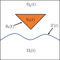
(a) Continuous domain

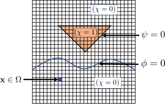
(b) FD/BP discretized domain

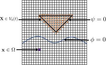
(c) FD/IB discretized domain

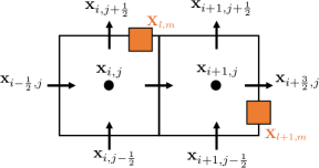
(d) Two grid cells & Lagrangian markers

Figure 1: 1(a) Sketch of the immersed structure interacting with liquid and gas phases in a rectangular domain. 1(b) Numerical discretization of the domain $\Omega$ into Eulerian grid cells ($\blacksquare$, purple) and the indicator function $\chi$ used in the FD/BP method to differentiate between the fluid and solid regions; $\chi=1$ inside the structure domain and $\chi=0$ in liquid and gas domains. 1(c) Numerical discretization of the domain $\Omega$ into Eulerian grid cells ($\blacksquare$, purple) and Lagrangian markers ($\blacksquare$, orange) for the FD/IB method. 1(d) Two Cartesian grid cells on which the components of the velocity field $\bm{\mathrm{u}}$ are approximated on the cell faces ($\rightarrow$, black); the pressure $p$ and level sets $\phi$ and $\psi$ are approximated on the cell center ($\bullet$, black); and the Lagrangian quantities are approximated on the marker points ($\blacksquare$, orange), which can arbitrarily cut through the Eulerian grid.

3.3 Lagrangian-Eulerian interaction for the FD/IB method

The transfer of quantities between the Eulerian and Lagrangian grids requires discrete approximations to the velocity interpolation and force spreading integrals described by Eqs. (3) and (4). It is convenient to use short-hand notation to denote these integrals. More specifically, the force spreading integral of Eq. (3) is denoted by $\bm{\mathrm{f}}=\bm{\mathrm{\mathcal{S}}}_{h}[\bm{\mathrm{X}}]\,\bm{\mathrm{F}}$, in which $\bm{\mathrm{\mathcal{S}}}_{h}[\bm{\mathrm{X}}]$ is the discrete version of the force-spreading operator. The velocity interpolation integral of Eq. (4) is denoted by $\bm{\mathrm{U}}=\bm{\mathrm{\mathcal{J}}}_{h}[\bm{\mathrm{X}}]\,\bm{\mathrm{u}}$, in which $\bm{\mathrm{\mathcal{J}}}_{h}[\bm{\mathrm{X}}]$ is the discrete version of velocity-interpolation operator. It can be shown that if $\bm{\mathrm{\mathcal{S}}}_{h}$ and $\bm{\mathrm{\mathcal{J}}}_{h}$ are taken to be adjoint operators, i.e. $\bm{\mathrm{\mathcal{S}}}_{h}=\bm{\mathrm{\mathcal{J}}}_{h}^{*}$, then the Lagrangian-Eulerian coupling conserves energy [30].

The discrete velocity interpolation of the staggered grid fluid velocity onto a specific configuration of Lagrangian markers (i.e. $\bm{\mathrm{U}}=\bm{\mathrm{\mathcal{J}}}_{h}[\bm{\mathrm{X}}]\bm{\mathrm{u}})$ reads

$$U_{l,m} =\sum_{\bm{\mathrm{x}}_{i-\frac{1}{2},j}\in\Omega}u_{i-\frac{1}{2},j}\delta_{h}\left(\bm{\mathrm{x}}_{i-\frac{1}{2},j}-\bm{\mathrm{X}}_{l,m}\right)\Delta x\Delta y,$$ (13)

$$V_{l,m} =\sum_{\bm{\mathrm{x}}_{i,j-\frac{1}{2}}\in\Omega}v_{i,j-\frac{1}{2}}\delta_{h}\left(\bm{\mathrm{x}}_{i,j-\frac{1}{2}}-\bm{\mathrm{X}}_{l,m}\right)\Delta x\Delta y,$$ (14)

The discrete spreading of a force density (defined on Lagrangian markers) onto faces of the staggered grid (i.e. $\bm{\mathrm{f}}=\bm{\mathrm{\mathcal{S}}}_{h}[\bm{\mathrm{X}}]\bm{\mathrm{F}}$) reads

$$(f_{1})_{i-\frac{1}{2},j} =\sum_{\bm{\mathrm{X}}_{l,m}\in V_{b}}(F_{1})_{l,m}\delta_{h}\left(\bm{\mathrm{x}}_{i-\frac{1}{2},j}-\bm{\mathrm{X}}_{l,m}\right)\Delta s_{1}\Delta s_{2},$$ (15)

$$(f_{2})_{i,j-\frac{1}{2}} =\sum_{\bm{\mathrm{X}}_{l,m}\in V_{b}}(F_{2})_{l,m}\delta_{h}\left(\bm{\mathrm{x}}_{i,j-\frac{1}{2}}-\bm{\mathrm{X}}_{l,m}\right)\Delta s_{1}\Delta s_{2}.$$ (16)

In the above expressions, $\delta_{h}(\bm{\mathrm{x}})$ denotes a regularized version of the two-dimensional Dirac delta function based on a four-point kernel function [30]. We use the same discrete Dirac delta function for both force-spreading and velocity interpolation operators, which ensures that $\bm{\mathrm{\mathcal{S}}}_{h}=\bm{\mathrm{\mathcal{J}}}_{h}^{*}$. We refer readers to [33, 30] for more details on various properties (including the spatial invariance property) and implementation of the grid transfer operations.

4 Solution methodology

In this section, we describe the full time-stepping scheme and the fluid-structure interaction algorithms employed for the FD/BP and FD/IB methods. We first describe the numerical elements common to both implementations, such as material property specification, level set advection and reinitialization, and incompressible Navier-Stokes solver for high density ratio multiphase flows. The main difference between the two FD methods is the fluid-structure coupling algorithm, which is detailed thereafter.

4.1 Material property specification

As described earlier in Sec. 2.2, the zero isocontours of $\phi(\bm{\mathrm{x}},t)$ and $\psi(\bm{\mathrm{x}},t)$ represent the liquid-air interface $\Gamma(t)$ and the boundary of the immersed structure $S_{b}(t)$, respectively. Using the signed distance property of $\phi$ and $\psi$, we define smoothed Heaviside functions that are regularized over $n_{\text{cells}}$ grid cells on either side of the interfaces (assuming $\Delta x=\Delta y)$,

$$\widetilde{H}^{\text{flow}}_{i,j} =\begin{cases}0,&\phi_{i,j}<-n_{\text{cells}}\Delta x,\\ \frac{1}{2}\left(1+\frac{1}{n_{\text{cells}}\Delta x}\phi_{i,j}+\frac{1}{\pi}\sin\left(\frac{\pi}{n_{\text{cells}}\Delta x}\phi_{i,j}\right)\right),&|\phi_{i,j}|\leq n_{\text{cells}}\Delta x,\\ 1,&\textrm{otherwise},\end{cases}$$ (17)

$$\widetilde{H}^{\text{body}}_{i,j} =\begin{cases}0,&\psi_{i,j}<-n_{\text{cells}}\Delta x,\\ \frac{1}{2}\left(1+\frac{1}{n_{\text{cells}}\Delta x}\psi_{i,j}+\frac{1}{\pi}\sin\left(\frac{\pi}{n_{\text{cells}}\Delta x}\psi_{i,j}\right)\right),&|\psi_{i,j}|\leq n_{\text{cells}}\Delta x,\\ 1,&\textrm{otherwise},\end{cases}$$ (18)

A given material property $\zeta$ (such as $\rho$ or $\mu$) is then prescribed in the whole domain using a two-step process. First, the material property in the “flowing” phase is set via the liquid-gas level set function

$$\zeta^{\text{flow}}_{i,j}=\zeta_{\text{l}}+(\zeta_{\text{g}}-\zeta_{\text{l}})\widetilde{H}^{\text{flow}}_{i,j}.$$ (19)

Next, the material property is set on cell centers throughout the computational domain, taking into account the solid phase 

$$\zeta_{i,j}^{\text{full}}=\zeta_{\text{s}}+(\zeta^{\text{flow}}_{i,j}-\zeta_{\text{s}})\widetilde{H}^{\text{body}}_{i,j}.$$ (20)

Without the loss of generality, the liquid phase is represented by the negative values of $\phi$ and the solid phase is represented by the negative $\psi$ values. Note that in the above equations, we have assumed that the number of transition cells is the same across $\Gamma$ and $S_{b}$. This is not a strict requirement of the numerical method, but it is true for all the cases considered in the present work.

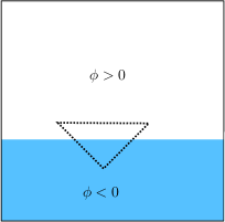
(a) Material properties in the “flowing” phases

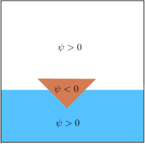
(b) Material properties in the entire domain

Figure 2: Sketch of the two-stage process for prescribing the material properties in the computational domain. 2(a) Density and viscosity are first prescribed in the “flowing” phase based on the liquid-gas level set function $\phi$ (—, black) and ignoring the body’s level set function $\psi$ (---, orange). 2(b) Density and viscosity are then corrected in the solid phase

In general, the signed distance property of $\phi$ and $\psi$ is not preserved under advection governed by Eqs. (7) and (8). Therefore, a reinitialization process is carried out at the end of each time step such that $\phi^{n+1}$ and $\psi^{n+1}$ represent a signed distance to their respective interfaces. This is described briefly in Appendix A, and in more detail by Nangia et al. [47].

4.2 Full time stepping scheme

We now describe the general time stepping scheme employed over the time interval $\left[t^{n},t^{n}+\Delta t\right]=\left[t^{n},t^{n+1}\right]$; within each time step, $n_{\text{cycles}}$ cycles of fixed-point iteration are used. In the present work, we always use $n_{\text{cycles}}=2$. Note that $k$ appears as a superscript to distinguish the cycle number. At the beginning of each time step we set $k=0$, with $\bm{\mathrm{u}}^{n+1,0}=\bm{\mathrm{u}}^{n}$, $p^{n+\frac{1}{2},0}=p^{n-\frac{1}{2}}$, $\phi^{n+1,0}=\phi^{n}$, $\psi^{n+1,0}=\psi^{n}$, and $\bm{\mathrm{X}}^{n+1,0}=\bm{\mathrm{X}}^{n}$. At the first time step $n=0$, these quantities are prescribed initial conditions. The midpoint, time-centered approximation to Lagrangian positions is given by $\bm{\mathrm{X}}^{n+\frac{1}{2},k}=\frac{1}{2}\left(\bm{\mathrm{X}}^{n+1,k}+\bm{\mathrm{X}}^{n}\right)$.

4.2.1 Scalar advection

The level set Eqs. (7) and (8) are discretized using a standard time-stepping approach as

$$\frac{\phi^{n+1,k+1}-\phi^{n}}{\Delta t}+Q\left(\bm{\mathrm{u}}^{n+\frac{1}{2},k},\phi^{n+\frac{1}{2},k}\right) =0,$$ (21)

$$\frac{\psi^{n+1,k+1}-\psi^{n}}{\Delta t}+Q\left(\bm{\mathrm{u}}^{n+\frac{1}{2},k},\psi^{n+\frac{1}{2},k}\right) =0,$$ (22)

in which $Q(\cdot,\cdot)$ represents a discretization of the linear advection term on cell centers via an explicit piecewise parabolic method. More specifically, the xsPPM7-limited version described in [60, 62] is employed. Homogenous Neumann boundary conditions are enforced for $\phi$ and $\psi$ on $\partial\Omega$ using a standard ghost cell treatment [63].

4.2.2 Incompressible Navier-Stokes solver: Conservative and consistent transport formulation

The conservative form of the incompressible Navier-Stokes equations Eqs. (1) and (2) are discretized as

$$\frac{\breve{\bm{\mathrm{\rho}}}^{n+1,k+1}\bm{\mathrm{u}}^{n+1,k+1}-{\bm{\mathrm{\rho}}}^{n}\bm{\mathrm{u}}^{n}}{\Delta t}+\bm{\mathrm{C}}^{n+1,k}=-\nabla_{h}p^{n+\frac{1}{2},k+1}+\left(\bm{\mathrm{L}}_{\mu}\bm{\mathrm{u}}\right)^{n+\frac{1}{2},k+1}+\bm{\mathrm{\wp}}^{n+1,k+1}\bm{\mathrm{g}}+\theta^{\text{FD}}\bm{\mathrm{f}}_{\text{c}}^{n+1,k+1},$$ (23)

$$\nabla_{h}\cdot\bm{\mathrm{u}}^{n+1,k+1}=0,$$ (24)

in which $\theta^{\text{FD}}=1$ for the FD/BP method and $\theta^{\text{FD}}=0$ for the FD/IB method, i.e., the Eulerian constraint forces are included when solving the INS momentum equation for the FD/BP method and ignored for the FD/IB method. The reason for ignoring constraint forces in the FD/IB method will become apparent later when we discuss its FSI algorithm. Similarly, the specific value of density $\bm{\mathrm{\wp}}$ field used to compute the gravitational body force $\bm{\mathrm{\wp}}\bm{\mathrm{g}}$ will be explained in the context of each fluid-structure coupling algorithm.

Note that $\left(\bm{\mathrm{L}}_{\mu}\bm{\mathrm{u}}\right)^{n+\frac{1}{2},k+1}=\frac{1}{2}\left[\left(\bm{\mathrm{L}}_{\mu}\bm{\mathrm{u}}\right)^{n+1,k+1}+\left(\bm{\mathrm{L}}_{\mu}\bm{\mathrm{u}}\right)^{n}\right]$ is a semi-implicit approximation to the viscous strain rate with $\left(\bm{\mathrm{L}}_{\mu}\right)^{n}=\nabla_{h}\cdot\left[\mu^{n}\left(\nabla_{h}\bm{\mathrm{u}}+\nabla_{h}\bm{\mathrm{u}}^{T}\right)^{n}\right]$, making the above time-stepping scheme with $n_{\text{cycles}}=2$ resemble a combination of Crank-Nicolson for the viscous terms and explicit midpoint rule for the convective term. The newest approximation to viscosity $\mu^{n+1,k+1}$ is obtained via the two-stage process described in Eqs. (19) and (20). The newest approximation to density $\breve{\bm{\mathrm{\rho}}}^{n+1,k+1}$ and the discretization of the convective term $\bm{\mathrm{C}}^{n+1,k}$ are computed such that they satisfy consistent mass/momentum transport, which is required to maintain numerical stability for air-water density ratios. We briefly describe this approach in Appendix B and refer the reader to Nangia et al. [47] for more details.

4.2.3 Fluid-structure coupling: FD/BP method

In the fictitious domain Brinkman penalization formulation, we retain the constraint force in the momentum equation by taking $\theta^{\text{FD}}=1$. The constraint/penalization force enforcing the rigid body motion is proportional to the difference between the desired structure velocity and the fluid velocity. For the time-stepping scheme it reads

$$\bm{\mathrm{f}}_{\text{c}}^{n+1,k+1}=\frac{\widetilde{\chi}}{K}\left(\bm{\mathrm{u}}_{\text{b}}^{n+1,k+1}-\bm{\mathrm{u}}^{n+1,k+1}\right),$$ (25)

in which $\widetilde{\chi}=1-\widetilde{H}^{\text{body}}$, $\widetilde{H}^{\text{body}}$ is the regularized structure Heaviside function (Eq. (18)) and $K\sim\mathcal{O}(10^{-8})$; this is sufficiently small to enforce the rigidity constraint in the structure domain, as described by prior studies [35, 64, 54]. The rigid body velocity $\bm{\mathrm{u}}_{\text{b}}$ in Eq. (25) can be expressed in terms of the translational $\bm{\mathrm{U}}_{\text{r}}$ and rotational $\bm{\mathrm{W}}_{\text{r}}$ center of mass velocities

$$\bm{\mathrm{u}}_{\text{b}}^{n+1,k+1}=\bm{\mathrm{U}}_{\text{r}}^{n+1,k+1}+\bm{\mathrm{W}}_{\text{r}}^{n+1,k+1}\times\left(\bm{\mathrm{x}}-\bm{\mathrm{X}}_{\text{com}}^{n+1,k+1}\right).$$ (26)

The center of mass velocities can be obtained in two distinct ways:

1. Fully prescribed motion:
   For some specified rigid body motion of the structure, i.e, the translational and rotational velocities of the body are known a priori, we can directly prescribe the velocity field at time step $n+1$ as

   $$\bm{\mathrm{u}}_{\text{b}}^{n+1,k+1}=\bm{\mathrm{U}}_{\text{r}}^{n+1}+\bm{\mathrm{W}}_{\text{r}}^{n+1}\times\left(\bm{\mathrm{x}}-\bm{\mathrm{X}}_{\text{com}}^{n+1}\right).$$ (27)

   This algorithm can be used to simulate one-way FSI problems such as flows over stationary bluff bodies or structures entering or exiting fluid-gas interfaces with known velocity.

2. Free-body motion:
   The rigid body velocity in this case can be obtained by integrating Newton’s second law of motion

   $$\text{M}_{\text{b}}\frac{\bm{\mathrm{U}}_{\text{r}}^{n+1,k+1}-\bm{\mathrm{U}}_{\text{r}}^{n}}{\Delta t} =\bm{\mathrm{\mathcal{F}}}^{n+1,k}+\text{M}_{\text{b}}\bm{\mathrm{g}},$$ (28)

   $$\bm{\mathrm{I}}_{\text{b}}\frac{\bm{\mathrm{W}}_{\text{r}}^{n+1,k+1}-\bm{\mathrm{W}}_{\text{r}}^{n}}{\Delta t} =\bm{\mathrm{\mathcal{M}}}^{n+1,k},$$ (29)

   in which $\text{M}_{\text{b}}$ is the mass, $\bm{\mathrm{I}}_{\text{b}}$ is the moment of inertia, $\bm{\mathrm{\mathcal{F}}}$ is the net hydrodynamic force, $\bm{\mathrm{\mathcal{M}}}$ is the net hydrodynamic torque and $\text{M}_{\text{b}}\bm{\mathrm{g}}$ is the net gravitational force acting on the body. Eqs. (28) and (29) are integrated using a forward-Euler scheme to compute $\bm{\mathrm{U}}_{\text{r}}^{n+1,k+1}$, $\bm{\mathrm{W}}_{\text{r}}^{n+1,k+1}$ and $\bm{\mathrm{X}}_{\text{com}}^{n+1,k+1}$. In practice we employ quaternions to integrate Eq. (29) in the initial reference frame, which avoids recomputing $\bm{\mathrm{I}}_{\text{b}}$ as the body rotates in a complex manner in three spatial dimensions.

We remark that since the gravitational force is included in the rigid body equation of motion (28), it is not necessary to include the volumetric gravity term $\bm{\mathrm{\rho}}_{\text{s}}\bm{\mathrm{g}}$ in the momentum equation (23). In fact, it is advantageous to just use $\bm{\mathrm{\rho}}^{\text{flow}}\bm{\mathrm{g}}$ to avoid spurious velocity currents near the fluid-solid interface due to high density gradients [47]. Similar arguments hold for the prescribed motion case. Therefore, we use $\bm{\mathrm{\wp}}\bm{\mathrm{g}}=\bm{\mathrm{\rho}}^{\text{flow}}\bm{\mathrm{g}}$ in Eq. (23) for the FD/BP method.

The hydrodynamic forces $\bm{\mathrm{\mathcal{F}}}$ and torques $\bm{\mathrm{\mathcal{M}}}$ acting on the body are calculated by directly summing pressure and viscous forces from the surrounding fluid on the areal elements of the body surface

$$\bm{\mathrm{\mathcal{F}}}^{n+1,k} =\sum_{f}\left(-p^{n+1,k}\bm{\mathrm{n}}_{f}+\mu_{f}\left(\nabla_{h}\bm{\mathrm{u}}^{n+1,k}+\left(\nabla_{h}\bm{\mathrm{u}}^{n+1,k}\right)^{T}\right)\cdot\bm{\mathrm{n}}_{f}\right)\Delta A_{f},$$ (30)

$$\bm{\mathrm{\mathcal{M}}}^{n+1,k} =\sum_{f}\left(\bm{\mathrm{x}}-\bm{\mathrm{X}}_{\text{com}}^{n+1,k}\right)\times\left(-p^{n+1,k}\bm{\mathrm{n}}_{f}+\mu_{f}\left(\nabla_{h}\bm{\mathrm{u}}^{n+1,k}+\left(\nabla_{h}\bm{\mathrm{u}}^{n+1,k}\right)^{T}\right)\cdot\bm{\mathrm{n}}_{f}\right)\Delta A_{f}.$$ (31)

In general, the surface boundary $S_{b}$ does not conform to the underlying Eulerian grid. Therefore, the above sums are evaluated by representing the body’s surface in a stair step manner using the grid cells adjacent to $S_{b}$. Fig. 3 depicts such a representation. More specifically, a grid face is considered to be a part of the structure boundary if the two grid cells containing it have structure level set $\psi$ values of opposite sign; the summation $\sum_{f}$ shown in Eqs (30) and (31) are over these particular grid faces. This simplifies the hydrodynamic force and torque computations significantly, since all of the required quantities are readily available or can be interpolated (by simple averaging) onto the Cartesian cell faces (e.g. face-centered pressure or viscosity $\mu_{f}$). This is one of the main advantages of fictitious domain methods over sharp interface methods: the solution variables are valid on either side of the interface. The latter methods require one-sided interpolations using computational geometry constructs.

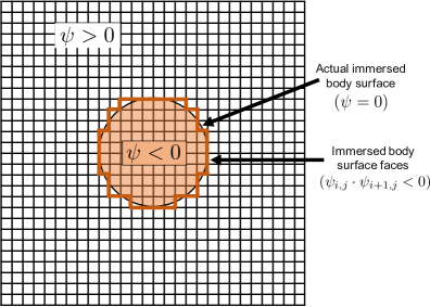
Figure 3: Discrete, stair step representation of the body’s surface $S_{b}$ on a Cartesian grid. For two adjacent cells with structure level set $\psi$ values of opposite sign, the common face with normal vector $\bm{\mathrm{n}}_{f}$ and surface area $\Delta A_{f}$ is used to evaluate the hydrodynamic force and torque integrals.

4.2.4 Fluid-structure coupling: FD/IB method

In the fictitious domain immersed boundary formulation, we ignore the constraint forces in the momentum equation by setting $\theta^{\text{FD}}=0$. Therefore, the velocity field computed by the flow solver using Eqs. (23) and (24) will not satisfy the rigid body motion constraints placed in the structure domain. However, the velocity field will be correct in the fluid domain. If $\widetilde{\bm{\mathrm{u}}}^{n+1,k+1}$ denotes the velocity solution obtained by ignoring the constraint forces, then to correct the velocity in $V_{b}(t)$ to $\bm{\mathrm{u}}^{n+1,k+1}$, we carry out the following projection step [33]

$$\breve{\bm{\mathrm{\rho}}}^{n+1,k+1}\left(\frac{\bm{\mathrm{u}}^{n+1,k+1}-\widetilde{\bm{\mathrm{u}}}^{n+1,k+1}}{\Delta t}\right)=\bm{\mathrm{f}}_{\text{c}}^{n+1,k+1}.$$ (32)

Similar to Brinkman penalization, the constraint force can be computed using the difference between two velocity fields: the desired body velocity and the interpolated uncorrected fluid velocity on the Lagrangian mesh $\Delta\bm{\mathrm{U}}^{n+1,k+1}_{l,m}$

$$\bm{\mathrm{f}}_{\text{c}}^{n+1,k+1} =\frac{\breve{\bm{\mathrm{\rho}}}^{n+1,k+1}}{\Delta t}\bm{\mathrm{\mathcal{S}}}_{h}\left[\bm{\mathrm{X}}^{n+\frac{1}{2},k}\right]\Delta\bm{\mathrm{U}}^{n+1,k+1}$$

$$=\frac{\breve{\bm{\mathrm{\rho}}}^{n+1,k+1}}{\Delta t}\bm{\mathrm{\mathcal{S}}}_{h}\left[\bm{\mathrm{X}}^{n+\frac{1}{2},k}\right]\left(\bm{\mathrm{U}}_{\text{b}}^{n+1,k+1}-\bm{\mathrm{\mathcal{J}}}_{h}\left[\bm{\mathrm{X}}^{n+\frac{1}{2},k}\right]\widetilde{\bm{\mathrm{u}}}^{n+1,k+1}\right),$$ (33)

which vanishes outside the structure domain. By correcting the fluid velocity in this way, we ensure that the Eulerian velocity in $V_{b}(t)$ approximately matches that of the solid’s Lagrangian velocity $\bm{\mathrm{U}}_{\text{b}}^{n+1,k+1}$. Combining the above two equations yields a simplified update equation for the Eulerian velocity field

$$\bm{\mathrm{u}}^{n+1,k+1}=\widetilde{\bm{\mathrm{u}}}^{n+1,k+1}+\bm{\mathrm{\mathcal{S}}}_{h}\left[\bm{\mathrm{X}}^{n+\frac{1}{2},k}\right]\left(\bm{\mathrm{U}}_{\text{b}}^{n+1,k+1}-\bm{\mathrm{\mathcal{J}}}_{h}\left[\bm{\mathrm{X}}^{n+\frac{1}{2},k}\right]\widetilde{\bm{\mathrm{u}}}^{n+1,k+1}\right).$$ (34)

We note that there is no guarantee that this corrected velocity will satisfy the divergence-free condition discretely; it is likely that $\nabla_{h}\cdot\bm{\mathrm{u}}^{n+1,k+1}\neq 0$. However, we have found that an additional divergence-free velocity projection is not necessary to obtain physically accurate results, corroborating previous investigations by Bhalla et al [33].

To compute $\bm{\mathrm{f}}_{\text{c}}^{n+1,k+1}$, we first determine $\bm{\mathrm{U}}_{\text{b}}^{n+1,k+1}$ in the Lagrangian frame. The rigid body velocity of each Lagrangian marker can be written as (omitting the time superscripts)

$$(\bm{\mathrm{U}}_{\text{b}})_{l,m}=\bm{\mathrm{U}}_{\text{r}}+\bm{\mathrm{W}}_{\text{r}}\times\bm{\mathrm{R}}_{l,m},$$ (35)

in which $\bm{\mathrm{R}}_{l,m}=\bm{\mathrm{X}}_{l,m}-\bm{\mathrm{X}}_{\text{com}}$ is the radius vector pointing from the center of mass to the Lagrangian marker position. Again considering the two FSI scenarios:

1. Fully prescribed motion:
   For problems in which the motion of the body is known a priori as a function of time, we can directly prescribe the Lagrangian velocity field at time step $n+1$ as

   $$(\bm{\mathrm{U}}_{\text{b}})^{n+1,k+1}_{l,m}=\bm{\mathrm{U}}_{\text{r}}^{n+1}+\bm{\mathrm{W}}_{\text{r}}^{n+1}\times\bm{\mathrm{R}}^{n+\frac{1}{2},k}_{l,m},$$ (36)

   which can be used to update the positions of the Lagrangian markers

   $$\bm{\mathrm{X}}_{l,m}^{n+1,k+1}=\bm{\mathrm{X}}_{l,m}^{n}+\Delta t(\bm{\mathrm{U}}_{\text{b}})^{n+\frac{1}{2},k+1}_{l,m}.$$ (37)

2. Free-body motion:
   For fully coupled problems in which the body moves as a result of the fluid-structure interaction, the Lagrangian velocity field at time step $n+1$ is determined by redistributing the linear and angular momentum [28, 53, 33] in the structure domain

   $$\text{M}_{\text{b}}\bm{\mathrm{U}}_{\text{r}}^{n+1,k+1} =\sum_{\bm{\mathrm{X}}_{l,m}\in V_{b}}\rho_{\text{s}}\left(\bm{\mathrm{\mathcal{J}}}_{h}\left[\bm{\mathrm{X}}^{n+\frac{1}{2},k}\right]\widetilde{\bm{\mathrm{u}}}^{n+1,k+1}\right)_{l,m}\Delta s_{1}\Delta s_{2},$$ (38)

   $$\bm{\mathrm{I}}_{\text{b}}\bm{\mathrm{W}}_{\text{r}}^{n+1,k+1} =\sum_{\bm{\mathrm{X}}_{l,m}\in V_{b}}\rho_{\text{s}}\bm{\mathrm{R}}^{n+\frac{1}{2},k}_{l,m}\times\left(\bm{\mathrm{\mathcal{J}}}_{h}\left[\bm{\mathrm{X}}^{n+\frac{1}{2},k}\right]\widetilde{\bm{\mathrm{u}}}^{n+1,k+1}\right)_{l,m}\Delta s_{1}\Delta s_{2}.$$ (39)

   The structure’s velocity and position are then updated via Eqs. (36) and (37).

Note that for fully prescribed motion, the gravitational force does not affect the body’s (specified) velocity. To avoid spurious flow currents near the fluid-structure interface (due to sharp density gradients) we simply use $\bm{\mathrm{\wp}}\bm{\mathrm{g}}=\bm{\mathrm{\rho}}^{\text{flow}}\bm{\mathrm{g}}$ for prescribed motion FSI problems. The free-body motion scenario requires special consideration. Because a momentum redistribution procedure is employed to obtain $\bm{\mathrm{U}}_{\text{r}}$ and $\bm{\mathrm{W}}_{\text{r}}$, the algorithm assumes that the uncorrected fluid momentum $\widetilde{\bm{\mathrm{u}}}$ is obtained by including all (including gravitational) body forces in the momentum equation (23). Therefore, the gravitational body force should account for the solid density and we use $\bm{\mathrm{\wp}}\bm{\mathrm{g}}=\bm{\mathrm{\rho}}^{\text{full}}\bm{\mathrm{g}}$ for free-body motion FSI problems. See [47] for more discussion.

The net hydrodynamic force $\bm{\mathrm{\mathcal{F}}}$ and torque $\bm{\mathrm{\mathcal{M}}}$ for the FD/IB method can be computed as a post-processing step using the Lagrangian quantities [46]

$$\bm{\mathrm{\mathcal{F}}}^{n+1} =\sum_{\bm{\mathrm{X}}_{l,m}\in V_{b}}\rho_{\text{s}}\left[\frac{\left(\bm{\mathrm{U}}_{\text{b}}\right)^{n+1}_{l,m}-\left(\bm{\mathrm{U}}_{\text{b}}\right)^{n}_{l,m}}{\Delta t}-\frac{\Delta\bm{\mathrm{U}}^{n+1}_{l,m}}{\Delta t}\right]\Delta s_{1}\Delta s_{2},$$ (40)

$$\bm{\mathrm{\mathcal{M}}}^{n+1} =\sum_{\bm{\mathrm{X}}_{l,m}\in V_{b}}\rho_{\text{s}}\bm{\mathrm{R}}^{n+1}_{l,m}\times\left[\frac{\left(\bm{\mathrm{U}}_{\text{b}}\right)^{n+1}_{l,m}-\left(\bm{\mathrm{U}}_{\text{b}}\right)^{n}_{l,m}}{\Delta t}-\frac{\Delta\bm{\mathrm{U}}^{n+1}_{l,m}}{\Delta t}\right]\Delta s_{1}\Delta s_{2},$$ (41)

in which the discrete approximations of the quantities on the right-hand side are readily available during each time step.

Finally, we remark that the above methodologies assume that all rigid-body degrees of freedom either are all fully prescribed (locked) or all undergoing free-body motion (unlocked). In our practical implementation, we are able to mix and match which degrees of freedom are locked and unlocked. We make use of this flexibility in the numerical examples presented in this work .

5 Comparison of the two fictitious domain methods

Below, we list some of the similarities and differences of the two previously described FD algorithms:

• Both methods extend the fluid momentum equation into the solid domain, which results in a valid solution on both sides of the structure interface.

• Both methods formulate the constraint force in terms of a difference between the desired body and fluid velocities. For a specific value of permeability $K=\Delta t/\breve{\bm{\mathrm{\rho}}}$, identical forms of the constraint force $\bm{\mathrm{f}}_{\text{c}}$ are obtained .

• The FD/BP method treats the constraint force implicitly, whereas the FD/IB method treats it explicitly. The explicit treatment of $\bm{\mathrm{f}}_{\text{c}}$ allows the use of an existing fluid solver without any modifications. The implicit Brinkman penalization method necessarily requires changes to an existing fluid solver infrastructure .

• The fully Eulerian nature of the FD/BP method is an attractive feature from a domain decomposition perspective, which can enable parallel scalability. In contrast, special load-balancing techniques must be employed to efficiently distribute Lagrangian and Eulerian data used in the FD/IB method.

• The momentum redistribution step of the FD/IB method avoids the need to compute hydrodynamic forces and torques on the immersed surface explicitly (which is a requirement of the FD/BP algorithm). The former approach requires Eulerian-Lagrangian interpolation and spreading routines, which may become expensive for large volumetric bodies.

• The FD/IB method works best for volumetric forces that are defined throughout the interior region of the structure. Incorporating point forces and torques that act only at certain points of the body (e.g. hinge forces or spring/damper forces) is not straightforward. Such forces and torques can be easily incorporated in Newton’s law of motion used in the FD/BP method.

6 Software implementation

The numerical algorithm described here is implemented within the IBAMR library [65], which is an open-source C++ simulation software focused on immersed boundary methods with adaptive mesh refinement. All of the numerical examples presented here are publicly available via https://github.com/IBAMR/IBAMR. IBAMR relies on SAMRAI [66, 67] for Cartesian grid management and the AMR framework. Linear and nonlinear solver support in IBAMR is provided by the PETSc library [68, 69, 70]. All of the example cases in the present work made use of distributed-memory parallelism using the Message Passing Interface (MPI) library. All of the example cases described in this section were carried out using 72 processors on the Fermi cluster at SDSU.

7 Numerical examples

We begin by simulating the challenging case of a two-dimensional, freely falling inclined wedge with three free degrees of freedom to validate the FD/BP method. We have extensively validated FD/IB implementations in previous work [33, 71, 46, 39, 40, 47, 72, 73] in the context of both two and three phase flows.

Next, we simulate water-entry and exit of a freely falling wedge and cylinder in two-spatial dimensions, and compare the fluid-structure dynamics obtained from FD/BP and FD/IB methods. For these cases, the only unlocked degree of freedom is the vertical ($y$) direction.

We use $n_{\text{cycles}}=2$ for both methods. Two grid cells of smearing $n_{\text{cells}}=2$ are used to transition between different material properties on either side of the interfaces. Water and air densities are taken to be $1000$ kg/m³ and $1.2$ kg/m³, respectively, and their respective viscosities are taken to be $10^{-3}$ Pa$\cdot$s and $1.8\times 10^{-5}$ Pa$\cdot$s. Surface tensions effects are neglected. No-slip boundary conditions are imposed along $\partial\Omega$.

7.1 Water-entry of a free falling inclined wedge

In this section, we consider the case of an inclined, 2D wedge-shaped object impacting an air-water interface. The wedge is initially rotated counterclockwise through a heel angle of $5^{\circ}$ as shown in Fig. 4. The isosceles triangle body has length $L=0.61$ m and a deadrise angle of $20^{\circ}$. Its mass and moment of inertia are $124$ kg and $8.85$ kg $\cdot$ m², respectively. The structure’s dimensions and material properties are chosen to match the experimental study conducted by Xu et al. [74]. Additionally, this case has been studied numerically using a weakly compressible smoothed particle hydrodynamics (SPH) method by Oger et al. [75], and an artificial compressibility method combined with Chimera grid-based Navier-Stokes solver by Nguyen et al. [76]. That is, the prior numerical studies [75, 76] simulate the compressible version of the Navier-Stokes equation in the low Mach number regime in contrast to the incompressible Navier-Stokes solver used in the present study.

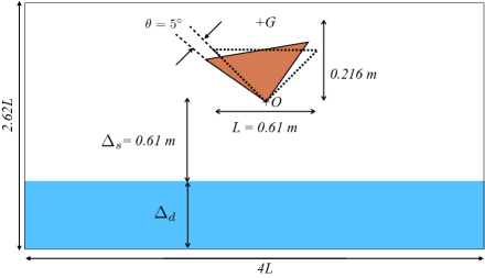
Figure 4: Schematic of a free falling wedge with an initial heel angle of $5^{\circ}$. $G$ is the center of mass location for the unrotated wedge, while $O$ is the initial location of the bottom vertex of the wedge. The distance $O-G=0.216$ m is the distance between the wedge tip and its COM point. Sketch is not to scale.

The computational domain is taken to be $\Omega=[0,4L]\times[0,2.62L]$, which is discretized by uniform computational grids. The initial distance between the bottom vertex of the wedge (point O in the Schematic 4) and the air-water interface is $\Delta_{s}=0.61$ m. We note that the domain dimensions and the depth of the initially quiescent water are not mentioned in prior experimental and numerical  investigations [74, 75, 76]. Therefore as a preliminary test case, four different water depths are considered: $\Delta_{d}=0.13$ m, $0.225$ m, $0.35$ m, and $0.45$ m and the results are compared to the experimental data of Xu et al. [74]. The domain is discretized by a $488\times 320$ grid (medium resolution), and a constant time step size of $\Delta t=2.5\times 10^{-5}$ is used. Fig. 5 shows the time evolution of vertical acceleration (normalized by $g=9.81$ m/s²) and angular acceleration for varying water depths. Note that the peak linear acceleration decreases with increased water depth [77]. Based on Fig. 5(a), it is evident that the best agreement with mean experimental data is achieved when simulating this problem using a water depth of $\Delta_{d}=0.13$ m. However, the wedge itself has a height of $0.11$ m, making this value of water depth inadequate for simulating long-term dynamics (in particular, experimental data are available up to a final time of around $t=0.45$ s). Therefore, we choose to use $\Delta_{d}=0.225$ m for the remaining cases in this section. Finally we note that although the peaks in our simulated angular accelerations match well with experimental data (Fig. 5(b)), there are some differences over the time interval $t=0.37$ s to $t=0.4$ s. We attribute these differences to three possibilities:

1. Compressibility effects during initial impact. Chen et al. [78] found that it can be important to consider compressibility of the water phase for problems involving substantial impact forces. Since our solver assumes incompressibility of liquid phases, fluid oozes from the sides of the object more quickly (compared to a compressible fluid), which may explain the faster angular dynamics observed in our simulations.

2. Minor differences in problem set up (such as domain boundaries or initial water depth) could also explain the deviations from the experimental data.

3. Unlike the linear acceleration data, which is reported as a mean of two experiments with a significant standard deviation, the angular acceleration data is reported from a single trial in Xu et al. [74]. It is unclear how repeatable these results are (i.e. multiple trials could exhibit large variability in results). In spite of some differences in the angular acceleration, we obtain an excellent match with the experimental data for angle of heel (see Fig. 6(a)).

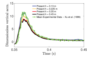
(a) Dimensionless vertical acceleration ($\ddot{y}/g)$

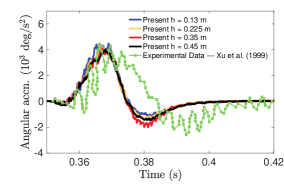
(b) Angular acceleration

Figure 5: Temporal evolution of 5(a) dimensionless vertical acceleration, and 5(b) angular acceleration for a 2D inclined wedge freely falling into water. (—) Present FD/BP simulation data for varying water depths; (–$\blacksquare$–, green) experimental data from Xu et al. [74].

For a fixed water depth $\Delta_{d}=0.225$ m, we now simulate this problem with three different mesh resolutions; a coarse grid ($244\times 160$ with $\Delta t=5\times 10^{-5})$, a medium grid ($488\times 320$ with $\Delta t=2.5\times 10^{-5}$) and a fine grid ($814\times 534$ with $\Delta t=1\times 10^{-5}$) are considered. Figs. 6(a) and 6(b) show time evolution of the wedge’s heel angle and vertical velocity, respectively, for all three mesh resolutions. For both quantities the solutions on the finest grid are in excellent agreement with the experimental data of Xu et al. [74], and grid convergence towards these data is also seen. In particular, a medium grid resolution that corresponds to approximately 120 grid cells per wedge length is adequate to resolve the FSI dynamics of a free-falling wedge. In Figs. 6(c) and 6(d), we show the dimensionless vertical acceleration and angular acceleration for the finest grid resolution as a function of time. Although the maximum vertical acceleration from the FD/BP method is slightly smaller than seen in experiments, the overall trend and values away from this peak match reasonably well. It is evident that the numerical simulations presented in Oger et al. [75] and Nguyen et al. [76] suffer from the same mismatch in peak linear acceleration. The peaks in angular acceleration are in decent agreement with the experimental study, although we again observe some differences in the trend over the time interval $t=0.37$ s to $t=0.4$ s even at the finest grid resolution. This implies that a converged solution for angular acceleration has been achieved for our simulations. The simulations from Oger et al. and Nguyen et al. are in much better agreement with the experiment, which we attribute to the fact that these authors considered compressibility effects in their numerical schemes. Finally in Fig. 7, we show the convergence of hydrodynamic vertical force and torque for three different grid resolutions. As expected, large impulses are seen as the wedge slams into the water just before $t=0.4$ s.

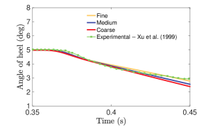
(a) Heel angle

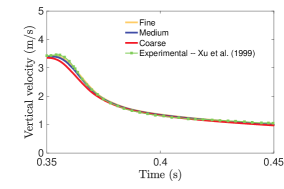
(b) Vertical velocity

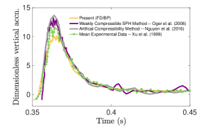
(c) Dimensionless vertical acceleration ($\ddot{y}/g)$

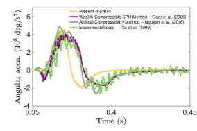
(d) Angular acceleration

Figure 6: Temporal evolution of 6(a) heel angle, 6(b) vertical velocity, 6(c) dimensionless vertical acceleration, and 6(d) angular acceleration, for a 2D inclined wedge freely falling into water. (—, yellow) Present FD/BP simulation data for a fine grid resolution $814\times 534$; (—, blue) Present FD/BP simulation data for a medium grid resolution $488\times 320$; (—, red) Present FD/BP simulation data for a coarse grid resolution $244\times 160$; (–$\blacksquare$–, green) experimental data from Xu et al. [74]; (—, purple) 2D simulation data from Oger et al. [75]; (—, grey) 2D simulation data from Nguyen et al. [76].

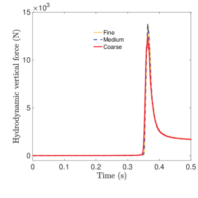
(a) Hydrodynamic vertical force

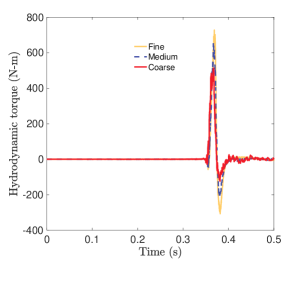
(b) Hydrodynamic torque

Figure 7: Temporal evolution of hydrodynamic 7(a) vertical force, and 7(b) torque for a 2D inclined wedge freely falling into water. (—, yellow) Present FD/BP simulation data for a fine grid resolution $814\times 534$; (---, blue) Present FD/BP simulation data for a medium grid resolution $488\times 320$; (—, red) Present FD/BP simulation data for a coarse grid resolution $244\times 160$.

Fig. 8 shows the evolution of fluid-structure interaction along with the vorticity generated by the inclined wedge for the medium and fine grid resolutions. As the wedge falls through the air phase, vortical structures are shed from the top corners. Upon impact these large scale vortices retain their structure on the medium grid, while they break down into smaller, satellite vortices on the fine grid. However, the overall trend of the vortex dynamics remains the same for the two grid resolutions. Asymmetric splashes emanate from the air-water interface at later times, as the fine grid resolves the small scale droplets. Note that the fine grid is able to capture emanating spray droplets better than the medium grid, which tends to dissipate them. The measured FSI quantities (heel angle, vertical velocity, and hydrodynamic moments) do not vary significantly between the grids, however. The overall dynamics are in relatively good agreement with the other numerical results in literature [75, 76].

(a) Fluid & structure medium grid

(b) Fluid & structure fine grid

(c) Medium grid, $t=0.220$ s

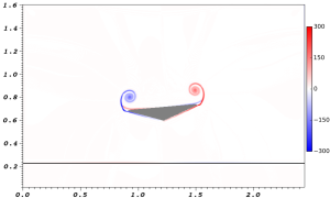
(d) Fine grid, $t=0.220$ s

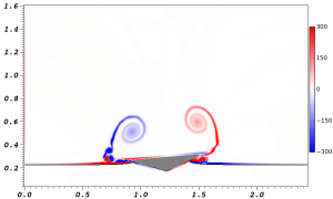
(e) Medium grid, $t=0.371$ s

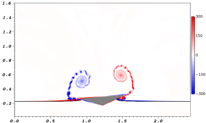
(f) Fine grid, $t=0.371$ s

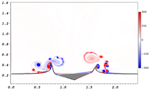
(g) Medium grid, $t=0.411$ s

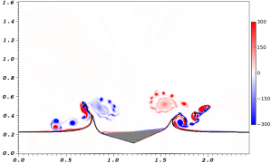
(h) Fine grid, $t=0.411$ s

Figure 8: Vorticity generated by a 2D inclined wedge freely falling into water at three different time instances using the FD/BP method on medium and fine grids. The plotted vorticity is in the range $-300$ to $300$ s^-1.

Finally, Fig. 9 shows the dimensionless pressure field $C_{p}=p/(\rho_{\text{l}}gL)$ as the wedge slams into the air-water interface. Immediately following impact high pressures are seen at the bottom tip of the wedge. This high pressure region shifts towards the left side of the body, which has more surface area covered with water. The results are in excellent agreement with the simulations shown in Nguyen et al. [76]. With this example, we have validated the accuracy the FD/BP method for simulating complex, high inertia FSI. Hereafter, we focus our attention on comparing and contrasting the FD/BP and FD/IB methodologies.

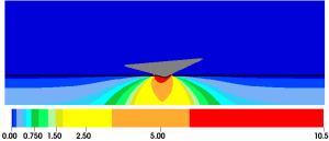
(a) $t=0.3570$ s

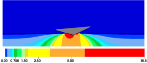
(b) $t=0.3608$ s

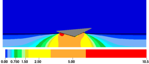
(c) $t=0.3676$ s

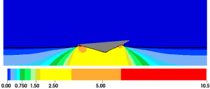
(d) $t=0.3726$ s

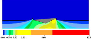
(e) $t=0.3826$ s

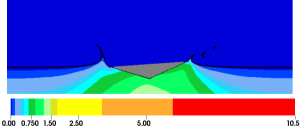
(f) $t=0.3950$ s

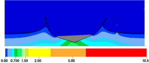
(g) $t=0.4500$ s

Figure 9: Dimensionless pressure field $C_{p}=p/(\rho_{\text{l}}gL)$ around a 2D inclined wedge freely falling into water at seven different time instances using the FD/BP method on fine grid.

7.2 Water-entry/exit of a free falling wedge

Next, we consider the problem of a wedge-shaped object impacting a pool of water. A 2D triangular body with top length $L=1.2$ m is placed within a computational domain of size $\Omega=[0,10L]\times[0,2.5L]$. The wedge is oriented with one of its vertices pointing downwards, making a $25^{\circ}$ deadrise angle with the horizontal. Water occupies the bottom third of the domain, while air occupies the remainder of the tank. The bottom point of the wedge is placed with initial position $(X_{0},Y_{0})=(5L,23L/12)$ and the wedge has a density of $\rho_{\text{s}}=466.6$ kg/m³. The free fall height of wedge is $\Delta s=13L/12$.

The 2D domain is discretized by a $1200\times 300$ uniform grid, which corresponds to 120 grid cells per wedge length. This grid resolution was found sufficient to resolve the FSI dynamics of a free-falling wedge in the previous section. A constant time step size of $\Delta t=6.25\times 10^{-5}$ s is used. Fig. 10 shows the time evolution of center of mass vertical position and velocity. The results are in good agreement with prior numerical [79] and experimental studies [8]. The wedge reaches a peak velocity in the air phase just before impacting the water surface. The vertical velocity keeps descending as it penetrates further into water. Eventually the buoyancy forces reverse the wedge’s velocity and it begins to exit the pool. Additionally, the hydrodynamic forces on the wedge in the vertical direction are compared. As seen in Fig. 10(c), the FD/IB method produces smooth forces compared to the FD/BP method. This is because evaluation of hydrodynamic forces for the FD/IB method is done in an extrinsic manner (Eqs. (40)-(41)). In contrast, the FD/BP method computes the forces in an intrinsic manner through direct stress evaluation involving derivatives of the velocity field. This is known (see Bergmann and Iollo [35]) to produce spurious oscillations in the force evaluation. In our prior work (Nangia et al. [46]) we proposed a moving control volume approach to obtain smooth forces by converting intrinsic integrals to extrinsic integrals over a moving Cartesian box. Others (Verma et al. [64] and Patel et al. [80]) have proposed to evaluate stress derivatives on a “lifted” surface that is two cells distance away from the original surface to avoid small scale oscillations for the FD/BP method.

Table 1 compares the time and velocity of impact obtained from FD/BP, FD/IB and Newton’s second law of motion. Aerodynamic air resistance is neglected from Newton’s law of motion. Both methods are in reasonable agreement with each other and also agree with the analytically predicted impact time and velocity. Fig. 12 compares the initial interfacial dynamics of wedge impact with prior experimental [81] and numerical studies [76]; decent agreement is seen. Fig. 11 shows the evolution of fluid-structure interaction along with the vorticity generated by the two methods. Upon impact, the FD/IB method sheds two counter-rotating vortices that are oriented inwards, whereas the FD/BP method, upon impact, sheds them in a slightly outward orientation (see time panel $t=0.5625$ s of Fig. 11). This is attributed to the differences in the impact forces and velocities predicted by the two methods. Another difference is in the fluid-structure interface handling in the two methods. This can also have some minor effects on the vortex shedding dynamics at high Reynolds numbers. There is also a slight delay in the vortical dynamics of the FD/BP method compared to the FD/IB method which can be explained by considering the lag in the impact time predicted by the former method. Similarly, the higher impact force of the FD/IB method as seen in Fig. 10(c) can be attributed to a higher impact velocity as compared to the FD/BP method.

Table 1: Water impact time and velocity of a free falling 2D wedge in air, computed using FD/BP, FD/IB, and Newton’s second law of motion.

Method	$t_{\text{impact}}$ (s)	$v_{\text{impact}}$ (m/s)
FD/BP	${0.5253}$	${4.7409}$
FD/IB	$0.5189$	$4.8347$
Newton’s law	$\sqrt{2\Delta s/g}=0.5148$	$gt_{\text{impact}}=5.0502$

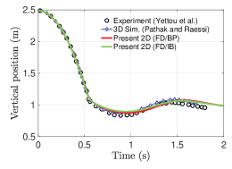
(a) Vertical position

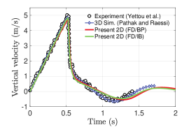
(b) Vertical velocity

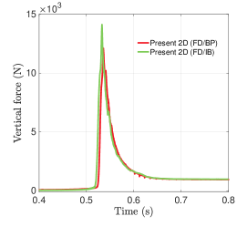
(c) Vertical force

Figure 10: Temporal evolution of 10(a) vertical position, 10(b) vertical velocity, and 10(c) vertical force on a 2D wedge freely falling in water. ($\circ$, black) experimental data from Yettou et al. [8]; ($\diamond$, blue) 3D simulation data from Pathak and Raessi [79]; (—, red) present FD/BP simulation data; (—, green) present FD/IB simulation data.

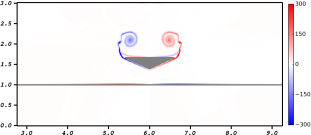
(a) FD/BP, $t=0.45$ s

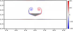
(b) FD/IB, $t=0.45$ s

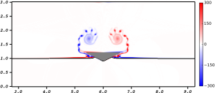
(c) FD/BP, $t=0.5625$ s

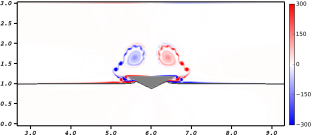
(d) FD/IB, $t=0.5625$ s

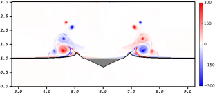
(e) FD/BP, $t=0.875$ s

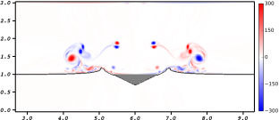
(f) FD/IB, $t=0.875$ s

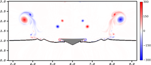
(g) FD/BP, $t=1.25$ s

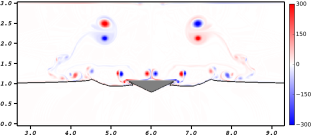
(h) FD/IB, $t=1.25$ s

Figure 11: Vorticity generated by a free falling 2D wedge at four different time instances using the FD/BP and FD/IB methods. The plotted vorticity is in the range $-300$ to $300$ s^-1.

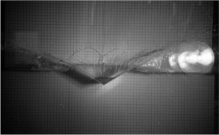
(a) Experiment [81]

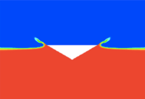
(b) Simulation [76]

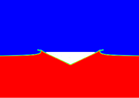
(c) Present FD/BP simulation

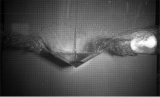
(d) Experiment [81]

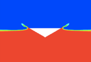
(e) Simulation [76]

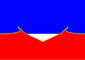
(f) Present FD/BP simulation

Figure 12: Visual comparisons of density and free surface: 12(a) and 12(d) experimental photographs from Greenhow and Lin [81]; 12(b) and 12(e) simulation snapshots from Nguyen et al. [76]; 12(c) and 12(f) simulation snapshots from the present the FD/BP method. Results from the FD/IB method are similar. Image permissions from the journals [81] and [76] pending.

7.3 Water-entry/exit of a free falling cylinder

In this section, we investigate the problem of a half-buoyant cylinder freely falling in water. This case has been studied numerically by Sun et al. [82] using a weakly compressible smoothed particle hydrodynamics (SPH) method, and by Patel and Natarajan [61] using an incompressible volume of fluid (VOF) solver. A circular cylinder of diameter $D=0.11$ m and density $\rho_{\text{s}}=500$ kg/m³ is placed in a two dimensional computational domain of size $\Omega=[0,20D]\times[0,12D]$ with initial center position $(X_{0},Y_{0})=(10D,8.05D)$. The domain is filled from $y=0$ to $y=3D$ with water; the remainder of the tank from $y=3D$ to $y=12D$ is filled with air. The cylinder has a free fall height of $\Delta s=4.55D$. The domain is discretized using a $880\times 528$ uniform grid, which corresponds to 44 cells per diameter. This grid resolution was found sufficient in our prior work for similar water-impact cases [47]. A constant time step size $\Delta t=10^{-5}$ s is used.

We again compare the rigid body dynamics of the cylinder obtained from the two methods. Figs. 13(a) and 13(b) show the time evolution of the center of mass vertical position and velocity, respectively. The hydrodynamic forces in the vertical direction obtained from the two methods are plotted in Fig. 13(c). Fig. 13(d) compares the variation of the depth of penetration as time progresses with the prior numerical studies [82, 61]. An excellent agreement is found between the FD/BP and SPH methods for most of the times. The FD/IB method gives slightly reduced penetration depth at later times compared to the FD/BP method. However, FSI results obtained from both FD implementations fall in the range of prior numerical studies.

Table 2 compares the time and velocity of impact obtained from FD/BP, FD/IB, prior numerical studies, and Newton’s second law of motion. Again, both methods are in reasonable agreement with each other and also agree well with the analytically predicted impact time and velocity. The impact time simulated by Patel and Natarajan underpredicts the expected value of $t_{\text{impact}}$. Sun et al. release the cylinder with an initial velocity of $v_{\text{impact}}$ (as predicted by Newton’s law) at the air-water interface and do not simulate the free-fall motion of the cylinder in the air phase. Fig. 14 shows the time evolution of interfacial dynamics using the two methods. The impacting cylinder produces distinct water jets while moving downward into the liquid. The initial impact of the cylinder produces ragged and non-smooth deformations in the separated water layer, as seen distinctly at $t=0.465$ s. These deformations are also observed in the weakly compressible SPH simulations of Sun et al. [83] and the incompressible VOF simulations of Patel and Natarajan [61]. Sun et al. attribute these deformations to negative pressure regions created in the receded water layer and numerically “fix” them by zeroing out the negative pressure. They refer this fix as a numerical model of water repellent coating on the cylinder surface. At around $t=0.52$ s, the cylinder reverses its direction of motion and pushes a layer of liquid along its surface as it rises up at $t=0.735$ s. Eventually, two opposite traveling waves on either side of the cylinder are formed when the cylinder enters back into the water for the second time. This can be distinctly seen at $t=1.365$ s. The slightly stronger water jets produced by the FD/IB method (compared to the FD/BP method) at the initial impact affects the interfacial dynamics at even later times. They also cause slight asymmetries on opposite sides of the cylinder at later times. In contrast, the FD/BP method maintains interfacial symmetry for most of the times shown.

Table 2: Water impact time and velocity of a free falling cylinder in air computed by FD/BP, FD/IB, Patel and Natarajan [61], Sun et al. [82], and Newton’s second law of motion.

Method	$t_{\text{impact}}$ (s)	$v_{\text{impact}}$ (m/s)
FD/BP	$0.3187$	$3.0690$
FD/IB	$0.3287$	$2.8936$
Patel and Natarajan [61]	$0.2997$	N/A
Sun et al. [82]	0.3194	3.1337
Newton’s law	$\sqrt{2\Delta s/g}=0.3194$	$gt_{\text{impact}}=3.1337$

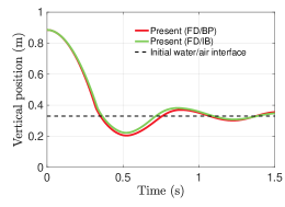
(a) Vertical position

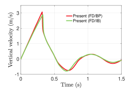
(b) Vertical velocity

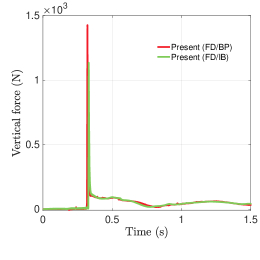
(c) Vertical force

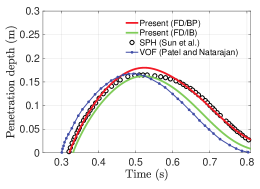
(d) Penetration depth

Figure 13: Temporal evolution of 13(a) vertical position, 13(b) vertical velocity, and 13(c) vertical force on a half-buoyant cylinder freely falling in water. (—, red) present FD/BP simulation data; ; (—, green) present FD/IB simulation data; ($\circ$, black) SPH simulation data from Sun et al. [82].

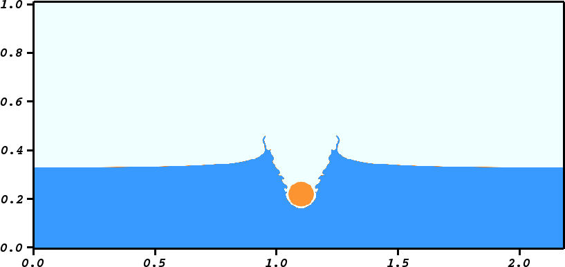
(a) FD/BP, $t=0.465$ s

(b) FD/IB, $t=0.465$ s

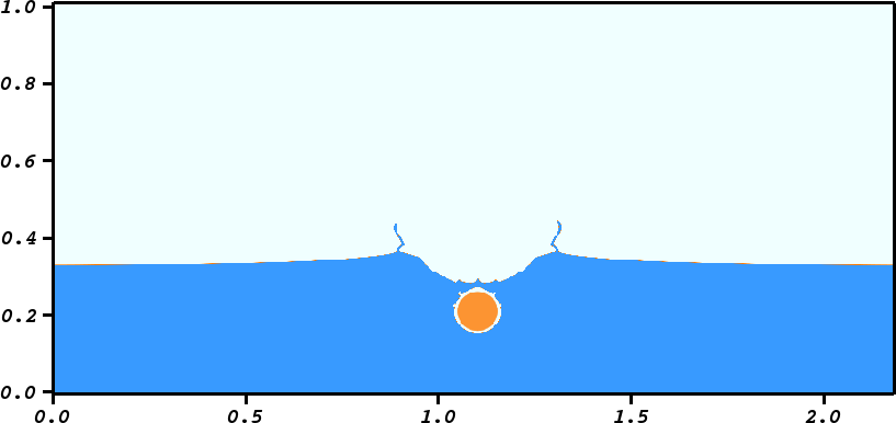
(c) FD/BP, $t=0.56$ s

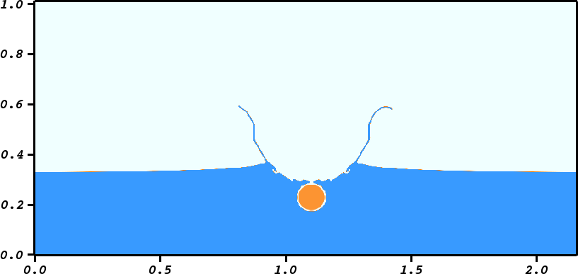
(d) FD/IB, $t=0.56$ s

(e) FD/BP, $t=0.735$ s

(f) FD/IB, $t=0.735$ s

(g) FD/BP, $t=1.365$ s

(h) FD/IB, $t=1.365$ s

Figure 14: Splash dynamics generated by a half-buoyant cylinder freely falling in water at four different time instances using the FD/BP and the FD/IB methods. Lighter blue color represents the air phase whereas darker blue color represents the water phase. The solid phase is shown in orange shade.

8 Comparison of computational costs

Finally, we briefly discuss and compare the computational costs associated with both methods. We consider the same two-dimensional test case described in the previous section: a half buoyant cylinder falling into an air-water interface. We discretize the problem on a coarser mesh of size $440\times 263$ so that the problem can be run relatively quickly on a single processor. A constant time step size of $\Delta t=1\times 10^{-5}$ is used. This test problem is simulated for $60$ time steps with both the FD/IB and FD/BP methods. The wall-clock time is measured for the final $50$ time steps of each simulation, and three experimental trials are conducted (and averaged) for each method. All of the solver options are identical across each trial. The total wall-clock time is broken up into four categories:

1. ‘INS Solver’, which corresponds to the operations required to solve the discrete fluid flow equations described by Eqs. (23) and (24) in Sec. 4.2.2.

2. ‘Level Set Update’, which corresponds to the operations required to discretely advect the level set variables (Eqs. (21) and (22) in Sec. 4.2.1, and reinitialize them to signed distances functions (see Appendix A).

3. ‘BP FSI Correction’ or ‘IB FSI Correction’, which correspond to the operations required to correct the fluid velocity in the domain occupied by the structure (described in Sec. 4.2.3 for the FD/BP method and in Sec. 4.2.4 for the FD/IB method.

4. ‘Other’, which corresponds to any operations not covered by the previous three descriptors. This includes allocation and deallocation of data structures and various pre- and post-processing function calls.

Fig. 15 shows the computation breakdown for each method. It is clear that discretely solving the fluid flow equations is by far the costliest operation, taking over $95\%$ of the total computation time for both methods. In contrast, the level set advection and reinitialization routines take very little wall-clock time; this is unsurprising since there are no Krylov iterative solvers employed in computing $\phi^{n+1}$ and $\psi^{n+1}$ – the update is purely explicit in nature. Finally, we note that the FSI correction for each method is incredibly fast, each taking only a fraction of a percent of total computation time. These results show that the present strong FSI coupling schemes are extremely efficient.

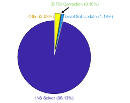
(a) FD/IB computation breakdown

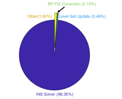
(b) FD/BP computation breakdown

Figure 15: Breakdown of computing time spent for the 15(a) FD/IB and 15(b) FD/BP methods. Note that the fraction of time spent for the FSI coupling computations is barely visible at this scale. All runs were carried out on a single processor.

Table 3 shows the average wall-clock time (in CPU units) required to compute each major component of the FD/BP and FD/IB algorithms. Unsurprisingly, the level set update takes approximately the same amount of time for both methods. Moreover, it is clear the the FSI coupling for the FD/BP method is more expensive than the FD/IB method. This can be attributed to the fact that the Brinkman penalization approach requires additional computations of hydrodynamic forces and torques (e.g. Eqs. (30) and (31)) and setting the matrix entries of the modified implicit fluid solver. Finally, it can be seen that the fluid solver for the FD/BP method is computationally more expensive than for the FD/IB method. This is because of the additional term present in the discrete INS equations due to the Brinkman penalization formulation ($\theta^{\text{FD}}=1$ in Eq. (23)). This term is treated implicitly, which changes the underlying discrete operator (and hence the linear solver convergence properties). For this particular example, the fluid solver for the FD/IB method converged in $1-2$ iterations each time step, while the fluid solver for the FD/BP (using the same solver settings) converged in $2-4$ iterations, explaining the disparity in wall-clock time.

We expect that the computational cost results would be similar for the other two cases described in this work. The FD/IB method outperforms the FD/BP method because the two-dimensional Lagrangian meshes considered in the present work are relatively simple and small. Moreover, we should note that the implementation of the IB transfer operators (e.g. spreading and interpolation) is quite mature; these computations have been well optimized and vectorized over the past two decades or so [65]. In contrast, the FD/BP has been recently implemented in IBAMR and we have not fully investigated speedup efforts. In particular, we believe that development of special multigrid smoothers (or other solver settings) for the implicit Brinkman penalization equations would help to reduce the number of Krylov iterations. These could make the computational cost of the FD/BP method comparable to the FD/IB method even for these small-scale 2D problems. We note that a more fair comparison of computational cost would be to compare timing data between the FD/IB method and an explicit version of the FD/BP method. The multigrid smoothers and an explicit FD/BP method will be explored in future endeavors.

For full, 3D engineering geometries (such as a wave energy converter device), we expect a critical problem size to exist at which the FD/BP method would outperform the FD/IB method. This is especially true when considering distributed memory parallelism; when two separate meshes exist (i.e. Lagrangian and Eulerian), two different domain decompositions must be maintained and mapped onto one another to achieve an efficient and scalable method. Even though the implicit FD/BP method will in general require more Krylov iterations, we expect that its purely Eulerian formulation will be advantageous for large engineering problems requiring scalable load balancing. The run time ratios and trends described in Fig. 15 and Table 3 would not necessarily hold for large, multi-processor runs. This will be the subject of future investigations.

Table 3: Average ($n=3$) wall-clock time required to compute each major component of the FD/BP and FD/IB algorithms. All runs were carried out on a single processor.

Method	INS Solver (CPU units)	Level Set Update (CPU units)	FSI Coupling (CPU units)
FD/BP	$541.79$	$2.82$	$0.79$
FD/IB	$229.57$	$2.73$	$0.38$

9 Conclusions

In this study, we described two implementations of the fictitious domain method capable of simulating water-entry/exit problems. One algorithm, based on the immersed boundary method, relied on an Eulerian description of the fluid variables and a Lagrangian representation of the immersed structure. The second algorithm, based on Brinkman penalization, was a purely Eulerian approach that imposed constraint forces implicitly rather than explicitly. We demonstrated that both methods can adequately resolve complex floating and splashing dynamics that are ubiquitous in practical marine engineering problems. They provide a good alternative to overset mesh based methods for simulating complex FSI problems.

For both methods, standard level set machinery was used to track air-water interfaces and the surface of the immersed body. The similarities and differences between the FD/BP and FD/IB methods were discussed, and several advantages and disadvantages of each technique were also described in Sec. 5. An efficient method for computing hydrodynamic forces and torques was detailed as a part of the FD/BP solution algorithm. We compared the techniques using two standard test cases: a half-buoyant, free-falling wedge and cylinder impacting an air-water interface. Both methods produced results that are in reasonable agreement with each other and compared favorably with prior results shown in literature.

The techniques described here have been implemented within the open-source IBAMR library. IBAMR is a flexible software infrastructure that provides support for several versions of the immersed boundary and fictitious domain methods. We are actively working on extending these methods to solve more complex problems. Future work includes implementation of a RANS or LES turbulence model and computational geometry algorithms to initialize and transport level set functions of more sophisticated solid geometries.

Appendix A Level set reinitialization

It is well-known that the signed distance property of $\phi$ and $\psi$ is disrupted under linear advection, Eqs. (7) and (8). Letting $\widetilde{\phi}^{n+1}$ denote the flow level set function following a single time step of transport through the interval $\left[t^{n},t^{n+1}\right]$, we need a procedure that reinitializes the field into a signed distance function $\phi^{n+1}$. This can be achieved by computing a steady-state solution to the Hamilton-Jacobi equation

$$\frac{\partial\phi}{\partial\tau}+\textrm{sgn}\left(\widetilde{\phi}^{n+1}\right)\left(\|\nabla\phi\|-1\right)=0,$$ (42)

$$\phi(\bm{\mathrm{x}},\tau=0)=\widetilde{\phi}^{n+1}(\bm{\mathrm{x}}),$$ (43)

which will yield a solution to the Eikonal equation $\|\nabla\phi\|=1$ at the end of each time step. More details on the specific discretization of Eqs. (42) and (43), which employs second-order ENO finite differences combined with a subcell-fix method described by Min [84], and an immobile interface condition described by Son [85], can be found in [52].

Since we consider simple geometries in this work, the solid level set $\psi^{n+1}$ is analytically calculated by using the new location of center of mass at $t^{n+1}$. For more complex structures, computational geometry techniques can be employed to compute the signed distance function.

Appendix B Discretization of the convective term: consistent mass/momentum transport

We use an explicit cubic upwind interpolation (CUI-limited) scheme [86, 87, 88] to approximate the $\bm{\mathrm{C}}^{n+1,k}$ nonlinear term in the momentum Eq. (23). A discretized mass balance equation is integrated directly on the faces of the staggered grid to obtain the newest approximation to density $\breve{\bm{\mathrm{\rho}}}^{n+1,k+1}$ in Eq. (23) from the previous time step and level set synchronized density field $\bm{\mathrm{\rho}}^{n}$ (obtained after averaging $\phi^{n}$ and $\psi^{n}$ onto faces):

$$\breve{\bm{\mathrm{\rho}}}^{(1)}=\bm{\mathrm{\rho}}^{n}-\Delta t\bm{\mathrm{R}}\left(\bm{\mathrm{u}}^{n}_{\text{adv}},\bm{\mathrm{\rho}}^{n}_{\text{lim}}\right),$$ (44)

$$\breve{\bm{\mathrm{\rho}}}^{(2)}=\frac{3}{4}\bm{\mathrm{\rho}}^{n}+\frac{1}{4}\breve{\bm{\mathrm{\rho}}}^{(1)}-\frac{1}{4}\Delta t\bm{\mathrm{R}}\left(\bm{\mathrm{u}}^{(1)}_{\text{adv}},\breve{\bm{\mathrm{\rho}}}^{(1)}_{\text{lim}}\right),$$ (45)

$$\breve{\bm{\mathrm{\rho}}}^{n+1,k+1}=\frac{1}{3}\bm{\mathrm{\rho}}^{n}+\frac{2}{3}\breve{\bm{\mathrm{\rho}}}^{(2)}-\frac{2}{3}\Delta t\bm{\mathrm{R}}\left(\bm{\mathrm{u}}^{(2)}_{\text{adv}},\breve{\bm{\mathrm{\rho}}}^{(2)}_{\text{lim}}\right).$$ (46)

A third-order accurate strong stability preserving Runge-Kutta (SSP-RK3) time integrator [89] is employed for the above update. Here $\bm{\mathrm{R}}\left(\bm{\mathrm{u}}_{\text{adv}},\bm{\mathrm{\varrho}}_{\text{lim}}\right)\approx\left[\left(\nabla\cdot\mbox{}\left(\bm{\mathrm{u}}_{\text{adv}}\bm{\mathrm{\varrho}}_{\text{lim}}\right)\right)_{i-\frac{1}{2},j},\left(\nabla\cdot\mbox{}\left(\bm{\mathrm{u}}_{\text{adv}}\bm{\mathrm{\varrho}}_{\text{lim}}\right)\right)_{i,j-\frac{1}{2}}\right]$ is an explicit CUI-limited approximation to the linear density advection term; $\bm{\mathrm{\varrho}}$ is either $\bm{\mathrm{\rho}}$ or $\breve{\bm{\mathrm{\rho}}}$. To clarify the various approximations to the density field, we make a distinction between $\breve{\bm{\mathrm{\rho}}}$, the density vector obtained via the SSP-RK3 integrator, and $\bm{\mathrm{\rho}}$, the density vector that is set from the level set fields. The subscript “adv” indicates the interpolated advective velocity on the faces of face-centered control volume, and the subscript “lim” indicates the limited value. Readers are referred to Nangia et al. [52] for details on obtaining advective and flux-limited fields. Notice that this density update procedure is occurring within the overall fixed-point iteration scheme.

In the SSP-RK3 update, we note that $\bm{\mathrm{u}}^{(1)}$ is an approximation to ${\bm{\mathrm{u}}}^{n+1}$, and $\bm{\mathrm{u}}^{(2)}$ is an approximation to ${\bm{\mathrm{u}}}^{n+\frac{1}{2}}$. Moreover, $\breve{\bm{\mathrm{\rho}}}^{(1)}$ is an approximation to $\breve{\bm{\mathrm{\rho}}}^{n+1}$, and $\breve{\bm{\mathrm{\rho}}}^{(2)}$ is an approximation to $\breve{\bm{\mathrm{\rho}}}^{n+\frac{1}{2}}$. We obtain these intermediate velocity and density approximations by using suitable interpolation and extrapolation procedures. For example, for the first cycle ($k=0$), the velocities are

$$\bm{\mathrm{u}}^{(1)}=2\bm{\mathrm{u}}^{n}-\bm{\mathrm{u}}^{n-1},$$ (47)

$$\bm{\mathrm{u}}^{(2)}=\frac{3}{2}\bm{\mathrm{u}}^{n}-\frac{1}{2}\bm{\mathrm{u}}^{n-1}.$$ (48)

For all remaining cycles ($k>0$), the velocities are

$$\bm{\mathrm{u}}^{(1)}={\bm{\mathrm{u}}}^{n+1,k},$$ (49)

$$\bm{\mathrm{u}}^{(2)}=\frac{3}{8}{\bm{\mathrm{u}}}^{n+1,k}+\frac{3}{4}\bm{\mathrm{u}}^{n}-\frac{1}{8}\bm{\mathrm{u}}^{n-1}.$$ (50)

To ensure consistent transport of mass and momentum fluxes, the convective derivative in Eq. (23) is given by

$$\bm{\mathrm{C}}\left(\bm{\mathrm{u}}^{(2)}_{\text{adv}},\breve{\bm{\mathrm{\rho}}}^{(2)}_{\text{lim}}\bm{\mathrm{u}}^{(2)}_{\text{lim}}\right)\approx\begin{bmatrix}\left(\nabla\cdot\mbox{}\left(\bm{\mathrm{u}}^{(2)}_{\text{adv}}\breve{\bm{\mathrm{\rho}}}^{(2)}_{\text{lim}}u^{(2)}_{\text{lim}}\right)\right)_{i-\frac{1}{2},j}\\ \left(\nabla\cdot\mbox{}\left(\bm{\mathrm{u}}^{(2)}_{\text{adv}}\breve{\bm{\mathrm{\rho}}}^{(2)}_{\text{lim}}v^{(2)}_{\text{lim}}\right)\right)_{i,j-\frac{1}{2}}\end{bmatrix},$$ (51)

which uses the same velocity $\bm{\mathrm{u}}^{(2)}_{\text{adv}}$ and density $\breve{\bm{\mathrm{\rho}}}^{(2)}_{\text{lim}}$ used to update $\breve{\bm{\mathrm{\rho}}}^{n+1}$ in Eq (46). This is the key step required to strongly couple the mass and momentum convective operators.

Bibliography

Bibliography

- [1] T. Tveitnes, A. Fairlie-Clarke, K. Varyani, An experimental investigation into the constant velocity water entry of wedge-shaped sections, Ocean Engineering 35 (14-15) (2008) 1463–1478.
- [2] G. Wu, H. Sun, Y. He, Numerical simulation and experimental study of water entry of a wedge in free fall motion, Journal of Fluids and Structures 19 (3) (2004) 277–289.
- [3] S. Howison, J. Ockendon, S. Wilson, Incompressible water-entry problems at small deadrise angles, Journal of Fluid Mechanics 222 (1991) 215–230.
- [4] X. Zhu, O. M. Faltinsen, C. Hu, Water entry and exit of a horizontal circular cylinder, Journal of Offshore Mechanics and Arctic Engineering 129 (4) (2007) 253–264.
- [5] M. Greenhow, Wedge entry into initially calm water, Applied Ocean Research 9 (4) (1987) 214–223.
- [6] M. Greenhow, Water-entry and-exit of a horizontal circular cylinder, Applied Ocean Research 10 (4) (1988) 191–198.
- [7] Z. Hou, T. Sun, X. Quan, G. Zhang, Z. Sun, Z. Zong, Large eddy simulation and experimental investigation on the cavity dynamics and vortex evolution for oblique water entry of a cylinder, Applied Ocean Research 81 (2018) 76–92.
- [8] E.-M. Yettou, A. Desrochers, Y. Champoux, Experimental study on the water impact of a symmetrical wedge, Fluid Dynamics Research 38 (1) (2006) 47.
- [9] T. von Kàrmàn, The impact on seaplane floats during landing, NACA TN 321.
- [10] Z. Dobrovol’Skaya, On some problems of similarity flow of fluid with a free surface, Journal of Fluid Mechanics 36 (4) (1969) 805–829.
- [11] I. Watanabe, Analytical expression of hydrodynamic impact pressure by matched asymptotic expansion technique, in: TRANSACTIONS OF THE WEST-JAPAN SOCIETY OF NAVAL ARCHITECTS 71, THE JAPAN SOCIETY OF NAVAL ARCHITECTS AND OCEAN ENGINEERS, 1986, pp. 77–85.
- [12] K. Kleefsman, G. Fekken, A. Veldman, B. Iwanowski, B. Buchner, A volume-of-fluid based simulation method for wave impact problems, Journal of Computational Physics 206 (1) (2005) 363–393.
- [13] Y. Zhang, Q. Zou, D. Greaves, D. Reeve, A. Hunt-Raby, D. Graham, P. James, X. Lv, A level set immersed boundary method for water entry and exit, Comm. Comput. Phys 8 (2) (2010) 265–288.
- [14] V. V. Nair, S. Bhattacharyya, Water entry and exit of axisymmetric bodies by CFD approach, Journal of Ocean Engineering and Science 3 (2) (2018) 156–174.
- [15] K. Takagi, Numerical evaluation of three-dimensional water impact by the displacement potential formulation, Journal of engineering mathematics 48 (3-4) (2004) 339–352.
- [16] C.-H. Lee, WAMIT theory manual, Massachusetts Institute of Technology, Department of Ocean Engineering, 1995.
- [17] C.-H. Lee, J. N. Newman, Wamit user manual, WAMIT, Inc.
- [18] Z. Shen, D. Wan, P. M. Carrica, Dynamic overset grids in OpenFOAM with application to KCS self-propulsion and maneuvering, Ocean Engineering 108 (2015) 287–306.
- [19] S. Bhushan, P. Carrica, J. Yang, F. Stern, Scalability studies and large grid computations for surface combatant using cfdship-iowa, The International Journal of High Performance Computing Applications 25 (4) (2011) 466–487.
- [20] N. G. Jacobsen, D. R. Fuhrman, J. Fredsøe, A wave generation toolbox for the open-source CFD library: OpenFOAM®, International Journal for Numerical Methods in Fluids 70 (9) (2012) 1073–1088.
- [21] T. H. Kasem, J. Sasaki, Multiphase modeling of wave propagation over submerged obstacles using weno and level set methods, Coastal Engineering Journal 52 (03) (2010) 235–259.
- [22] L. Chen, J. Zang, A. Hillis, G. Morgan, A. Plummer, Numerical investigation of wave–structure interaction using OpenFOAM, Ocean Engineering 88 (2014) 91–109.
- [23] ANSYS Fluent 12.0 Theory Guide (2009).
- [24] STAR-CCM+ Guide User Version (7.04) (2012).
- [25] P. Higuera, J. L. Lara, I. J. Losada, Realistic wave generation and active wave absorption for Navier–Stokes models: Application to OpenFOAM®, Coastal Engineering 71 (2013) 102–118.
- [26] P. M. Carrica, R. V. Wilson, R. W. Noack, F. Stern, Ship motions using single-phase level set with dynamic overset grids, Computers & fluids 36 (9) (2007) 1415–1433.
- [27] A. L. Facci, M. Porfiri, S. Ubertini, Three-dimensional water entry of a solid body: A computational study, Journal of Fluids and Structures 66 (2016) 36–53.
- [28] N. A. Patankar, P. Singh, D. D. Joseph, R. Glowinski, T.-W. Pan, A new formulation of the distributed Lagrange multiplier/fictitious domain method for particulate flows, International Journal of Multiphase Flow 26 (9) (2000) 1509–1524.
- [29] N. Sharma, N. A. Patankar, A fast computation technique for the direct numerical simulation of rigid particulate flows, Journal of Computational Physics 205 (2) (2005) 439–457.
- [30] C. S. Peskin, The immersed boundary method, Acta Numer 11 (2002) 479–517.
- [31] P. Angot, C.-H. Bruneau, P. Fabrie, A penalization method to take into account obstacles in incompressible viscous flows, Numerische Mathematik 81 (4) (1999) 497–520.
- [32] G. Carbou, P. Fabrie, et al., Boundary layer for a penalization method for viscous incompressible flow, Advances in Differential equations 8 (12) (2003) 1453–1480.
-
[33]
A. P. S. Bhalla, R. Bale, B. E. Griffith, N. A. Patankar,
A
unified mathematical framework and an adaptive numerical method for
fluid-structure interaction with rigid, deforming, and elastic bodies, J
Comput Phys 250 (1) (2013) 446–476.
doi:10.1016/j.jcp.2013.04.033.
URL http://linkinghub.elsevier.com/retrieve/pii/S0021999113003173 - [34] M. Vanella, E. Balaras, Short note: A moving-least-squares reconstruction for embedded-boundary formulations, Journal of Computational Physics 228 (18) (2009) 6617–6628.
- [35] M. Bergmann, A. Iollo, Modeling and simulation of fish-like swimming, Journal of Computational Physics 230 (2) (2011) 329–348.
- [36] R. Mittal, G. Iaccarino, Immersed boundary methods, Annu. Rev. Fluid Mech. 37 (2005) 239–261.
- [37] D. B. Stein, R. D. Guy, B. Thomases, Immersed boundary smooth extension: a high-order method for solving pde on arbitrary smooth domains using fourier spectral methods, Journal of Computational Physics 304 (2016) 252–274.
- [38] D. B. Stein, R. D. Guy, B. Thomases, Immersed boundary smooth extension (IBSE): A high-order method for solving incompressible flows in arbitrary smooth domains, Journal of Computational Physics 335 (2017) 155–178.
- [39] B. Kallemov, A. Bhalla, B. Griffith, A. Donev, An immersed boundary method for rigid bodies, Communications in Applied Mathematics and Computational Science 11 (1) (2016) 79–141.
- [40] F. Balboa Usabiaga, B. Kallemov, B. Delmotte, A. Bhalla, B. Griffith, A. Donev, Hydrodynamics of suspensions of passive and active rigid particles: a rigid multiblob approach, Communications in Applied Mathematics and Computational Science 11 (2) (2017) 217–296.
- [41] Y. Feldman, Y. Gulberg, An extension of the immersed boundary method based on the distributed Lagrange multiplier approach, Journal of Computational Physics 322 (2016) 248–266.
- [42] I. Borazjani, L. Ge, T. Le, F. Sotiropoulos, A parallel overset-curvilinear-immersed boundary framework for simulating complex 3D incompressible flows, Computers & Fluids 77 (2013) 76–96.
- [43] R. Mittal, H. Dong, M. Bozkurttas, F. Najjar, A. Vargas, A. von Loebbecke, A versatile sharp interface immersed boundary method for incompressible flows with complex boundaries, J Comput Phys 227 (10) (2008) 4825–4852.
- [44] Y.-H. Tseng, J. H. Ferziger, A ghost-cell immersed boundary method for flow in complex geometry, J Comput Phys 192 (2) (2003) 593–623.
- [45] A. Calderer, S. Kang, F. Sotiropoulos, Level set immersed boundary method for coupled simulation of air/water interaction with complex floating structures, Journal of Computational Physics 277 (2014) 201–227.
- [46] N. Nangia, H. Johansen, N. A. Patankar, A. P. S. Bhalla, A moving control volume approach to computing hydrodynamic forces and torques on immersed bodies, Journal of Computational Physics 347 (2017) 437–462.
- [47] N. Nangia, N. A. Patankar, A. P. S. Bhalla, A DLM immersed boundary method based wave-structure interaction solver for high density ratio multiphase flows, Journal of Computational Physics, In press.
- [48] M. Raessi, A level set based method for calculating flux densities in two-phase flows, Annual Research Briefs (Center for Turbulence Research, Stanford).
- [49] M. Raessi, H. Pitsch, Consistent mass and momentum transport for simulating incompressible interfacial flows with large density ratios using the level set method, Computers & Fluids 63 (2012) 70–81.
- [50] O. Desjardins, V. Moureau, Methods for multiphase flows with high density ratio, Center for Turbulent Research, Summer Programm 2010 (2010) 313–322.
- [51] S. Ghods, M. Herrmann, A consistent rescaled momentum transport method for simulating large density ratio incompressible multiphase flows using level set methods, Physica Scripta 2013 (T155) (2013) 014050.
- [52] N. Nangia, B. E. Griffith, N. A. Patankar, A. P. S. Bhalla, A robust incompressible Navier-Stokes solver for high density ratio multiphase flows, Journal of Computational Physics 390 (2019) 548–594.
- [53] A. A. Shirgaonkar, M. A. MacIver, N. A. Patankar, A new mathematical formulation and fast algorithm for fully resolved simulation of self-propulsion, Journal of Computational Physics 228 (7) (2009) 2366–2390.
- [54] M. Gazzola, O. V. Vasilyev, P. Koumoutsakos, Shape optimization for drag reduction in linked bodies using evolution strategies, Computers & Structures 89 (11-12) (2011) 1224–1231.
- [55] S. Osher, J. A. Sethian, Fronts propagating with curvature-dependent speed: algorithms based on hamilton-jacobi formulations, Journal of Computational Physics 79 (1) (1988) 12–49.
- [56] J. A. Sethian, P. Smereka, Level set methods for fluid interfaces, Annual review of fluid mechanics 35 (1) (2003) 341–372.
- [57] M. Sussman, P. Smereka, S. Osher, A level set approach for computing solutions to incompressible two-phase flow, Journal of Computational Physics 114 (1) (1994) 146–159.
- [58] D. L. Chopp, Computing minimal surfaces via level set curvature flow, Journal of Computational Physics 106 (1993) 77–91.
- [59] M. Cai, A. Nonaka, J. B. Bell, B. E. Griffith, A. Donev, Efficient variable-coefficient finite-volume stokes solvers, Communications in Computational Physics 16 (5) (2014) 1263–1297.
- [60] B. E. Griffith, An accurate and efficient method for the incompressible Navier-Stokes equations using the projection method as a preconditioner, Journal of Computational Physics 228 (20) (2009) 7565–7595.
- [61] J. K. Patel, G. Natarajan, Diffuse interface immersed boundary method for multi-fluid flows with arbitrarily moving rigid bodies, Journal of Computational Physics 360 (2018) 202–228.
- [62] W. J. Rider, J. A. Greenough, J. R. Kamm, Accurate monotonicity-and extrema-preserving methods through adaptive nonlinear hybridizations, Journal of Computational Physics 225 (2) (2007) 1827–1848.
- [63] F. H. Harlow, J. E. Welch, Numerical calculation of time-dependent viscous incompressible flow of fluid with free surface, The physics of fluids 8 (12) (1965) 2182–2189.
- [64] S. Verma, G. Abbati, G. Novati, P. Koumoutsakos, Computing the force distribution on the surface of complex, deforming geometries using vortex methods and brinkman penalization, International Journal for Numerical Methods in Fluids 85 (8) (2017) 484–501.
- [65] IBAMR: An adaptive and distributed-memory parallel implementation of the immersed boundary method, https://github.com/IBAMR/IBAMR.
- [66] R. D. Hornung, S. R. Kohn, Managing application complexity in the SAMRAI object-oriented framework, Concurrency Comput Pract Ex 14 (5) (2002) 347–368.
- [67] SAMRAI: Structured Adaptive Mesh Refinement Application Infrastructure, http://www.llnl.gov/CASC/SAMRAI.
- [68] S. Balay, W. D. Gropp, L. C. McInnes, B. F. Smith, Efficient management of parallelism in object oriented numerical software libraries, in: E. Arge, A. M. Bruaset, H. P. Langtangen (Eds.), Modern Software Tools in Scientific Computing, Birkhäuser Press, 1997, pp. 163–202.
-
[69]
S. Balay, S. Abhyankar, M. F. Adams, J. Brown, P. Brune, K. Buschelman,
L. Dalcin, V. Eijkhout, W. D. Gropp, D. Kaushik, M. G. Knepley, L. C.
McInnes, K. Rupp, B. F. Smith, S. Zampini, H. Zhang,
PETSc users manual, Tech. Rep.
ANL-95/11 - Revision 3.6, Argonne National Laboratory (2015).
URL http://www.mcs.anl.gov/petsc -
[70]
S. Balay, S. Abhyankar, M. F. Adams, J. Brown, P. Brune, K. Buschelman,
L. Dalcin, V. Eijkhout, W. D. Gropp, D. Kaushik, M. G. Knepley, L. C.
McInnes, K. Rupp, B. F. Smith, S. Zampini, H. Zhang,
PETSc Web page,
http://www.mcs.anl.gov/petsc (2015).
URL http://www.mcs.anl.gov/petsc - [71] A. P. S. Bhalla, B. E. Griffith, N. A. Patankar, A forced damped oscillation framework for undulatory swimming provides new insights into how propulsion arises in active and passive swimming, PLoS computational biology 9 (6) (2013) e1003097.
- [72] A. P. S. Bhalla, R. Bale, B. E. Griffith, N. A. Patankar, Fully resolved immersed electrohydrodynamics for particle motion, electrolocation, and self-propulsion, Journal of Computational Physics 256 (2014) 88–108.
- [73] T. Dombrowski, S. K. Jones, G. Katsikis, A. P. S. Bhalla, B. E. Griffith, D. Klotsa, Transition in swimming direction in a model self-propelled inertial swimmer, Physical Review Fluids 4 (2) (2019) 021101.
- [74] L. Xu, A. Troesch, R. Peterson, Asymmetric hydrodynamic impact and dynamic response of vessels, Journal of Offshore Mechanics and Arctic Engineering 121 (2) (1999) 83–89.
- [75] G. Oger, M. Doring, B. Alessandrini, P. Ferrant, Two-dimensional SPH simulations of wedge water entries, Journal of computational physics 213 (2) (2006) 803–822.
- [76] V.-T. Nguyen, D.-T. Vu, W.-G. Park, C.-M. Jung, Navier–Stokes solver for water entry bodies with moving Chimera grid method in 6 DOF motions, Computers & Fluids 140 (2016) 19–38.
- [77] H. Ghazizade-Ahsaee, A. Nikseresht, Numerical solution of the asymmetric water impact of a wedge in three degrees of freedom, China Ocean Engineering 27 (3) (2013) 313–322.
- [78] C. Chen, X. Yuan, X. Liu, J. Dang, Experimental and numerical study on the oblique water-entry impact of a cavitating vehicle with a disk cavitator, International Journal of Naval Architecture and Ocean Engineering 11 (1) (2019) 482–494.
- [79] A. Pathak, M. Raessi, A 3D, fully Eulerian, VOF-based solver to study the interaction between two fluids and moving rigid bodies using the fictitious domain method, Journal of Computational Physics 311 (2016) 87–113.
- [80] N. K. Patel, A. P. S. Bhalla, N. A. Patankar, A new constraint-based formulation for hydrodynamically resolved computational neuromechanics of swimming animals, Journal of Computational Physics 375 (2018) 684–716.
- [81] M. Greenhow, W.-M. Lin, Nonlinear-free surface effects: experiments and theory, Tech. rep., Massachusetts Inst Of Tech Cambridge Dept Of Ocean Engineering (1983).
- [82] P. Sun, F. Ming, A. Zhang, Numerical simulation of interactions between free surface and rigid body using a robust SPH method, Ocean Engineering 98 (2015) 32–49.
- [83] P. Sun, A.-M. Zhang, S. Marrone, F. Ming, An accurate and efficient SPH modeling of the water entry of circular cylinders, Applied Ocean Research 72 (2018) 60–75.
- [84] C. Min, On reinitializing level set functions, Journal of Computational Physics 229 (8) (2010) 2764–2772.
- [85] G. Son, A level set method for incompressible two-fluid flows with immersed solid boundaries, Numerical Heat Transfer, Part B 47 (5) (2005) 473–489.
- [86] P. Roe, M. Baines, Algorithms for advection and shock problems, in: Numerical Methods in Fluid Mechanics, 1982, pp. 281–290.
- [87] N. P. Waterson, H. Deconinck, Design principles for bounded higher-order convection schemes–a unified approach, Journal of Computational Physics 224 (1) (2007) 182–207.
- [88] J. K. Patel, G. Natarajan, A generic framework for design of interface capturing schemes for multi-fluid flows, Computers & Fluids 106 (2015) 108–118.
- [89] S. Gottlieb, C.-W. Shu, E. Tadmor, Strong stability-preserving high-order time discretization methods, SIAM review 43 (1) (2001) 89–112.