Plasma living in a curved surface at some special temperature

Abstract

The simplest statistical mechanics model of a Coulomb plasma in two spatial dimensions admits an exact analytic solution at some special temperature in several (curved) surfaces. We present in a unifying perspective these solutions for the (non-quantum) plasma, made of point particles carrying an absolute charge $e$, in thermal equilibrium at a temperature $T=e^{2}/2k_{B}$, with $k_{B}$ Boltzmann’s constant, discussing the importance of having an exact solution, the role of the curvature of the surface, and the densities of the plasma.

Part I Introduction

The physics of fluids of particles living in (curved) surfaces is a well known chapter of surface physics. It arises in situations in which particles are adsorbed or confined on a substrate with nonzero curvature, be it the wall of a porous material, or a membrane, a vesicle, a micelle for example made of ampiphilic surfactant molecules such as lipids, or a biological membrane, or the surface of a large solid particle, or an interface in an oil-water emulsion Fantoni et al. (2012). On the other hand it often occurs that by lowering the number of spatial dimensions, the statistical mechanics problem of a given fluid in the whole space, greatly simplifies, to the point of becoming, in certain cases, exactly solvable analytically in the continuum. A relevant feature of such low dimensional exactly solvable fluids is that they often play an important role as exact standards and guides to test approximate solutions and numerical experiments for (higher dimensional) fluid’s models. In a more general context, the few exact analytical results have helped form new qualitative insights given by sum rules and in clarifying the nature of the long distance asymptotic decay of the truncated two (or more) particle distribution functions Martin (1988); Tarjus et al. (2010).

In the statistical physics of continuous fluids, those where the particles are allowed to move in a continuous space, one finds examples of exactly solvable ones especially among the non-quantum in lower dimensions (one and two).

Coulomb systems March and Tosi (1984); Henderson et al. (2005) such as plasmas, electrolytes, or generally ionic materials are made of charged particles interacting through the long-range Coulomb law. They are an important chapter of ionic condensed matter (in systems like molten salts, transition metal ions in solution, molten alkali halides, $\ldots$) or ionic soft matter (in systems like natural or synthetic saline environments like aqueous and non aqueous electrolyte solutions, polyelectrolytes, colloidal suspensions, $\ldots$). The simplest model of a Coulomb system is the one-component plasma (OCP), also called jellium: an assembly of identical point charges of charge $e$, embedded in a neutralizing uniform background of the opposite sign. Here we consider the classical (i.e. non-quantum) equilibrium statistical mechanics of the OCP. According to the proof of Sari and Merlini Sari and Merlini (1976) which goes through “H-stability” and the “cheese theorem”, the OCP must have a well behaved thermodynamic limit. Though this model might seem, at first sight, oversimplified as to bear little resemblance to molten salts or liquid metals, it is nevertheless of great value in clarifying general effects which emerge as a direct consequence of long-range Coulomb’s interaction. This model constitutes the basic link between the microscopic description and the phenomenology of ionic condensed and soft matter.

The two-dimensional version (2D OCP) of the OCP has been much studied. Provided that the Coulomb potential due to a point-charge is defined as the solution of the Poisson equation “in” a two-dimensional world, i.e., is a logarithmic function $-\ln r$ of the distance $r$ to that point-charge, the 2D OCP mimics many generic properties of the three-dimensional Coulomb systems. In this case the electric field lines are not allowed to leave the surface as it happens in the satirical novella of Edwin Abbott Abbott Abbott (1884). Of course, this toy logarithmic model does not describe real charged particles, such as electrons, confined on a surface, which nevertheless interact through the three dimensional Coulomb potential $1/r$. One motivation for studying the 2D OCP is that its equilibrium statistical mechanics is analytically exactly solvable at one special temperature: both the thermodynamical quantities and the correlation functions are available.

The OCP is exactly solvable in one dimension Edwards and Lenard (1962); Fantoni (2016). In two dimensions, Jancovici and Alastuey Ginibre (1965); Metha (1967); Jancovici (1981a); Alastuey and Jancovici (1981) proved that the OCP is exactly solvable analytically at a special value of the coupling constant, $\Gamma=\beta e^{2}=2$ where $\beta=1/k_{B}T$ with $k_{B}$ Boltzmann’s constant and $T$ the absolute temperature, on a plane. Since then, a growing interest in two-dimensional plasmas has lead to study this system on various flat geometries Rosinberg and Blum (1984); Jancovici et al. (1994); Jancovici and Téllez (1996) and two-dimensional curved surfaces like the cylinder Choquard (1981); Choquard et al. (1983), the sphere Caillol (1981); Téllez and Forrester (1999); Jancovici (2000); Salazar and Téllez (2016), the the pseudosphere Jancovici and Téllez (1998); Fantoni et al. (2003); Jancovici and Téllez (2004), and Flamm paraboloid Fantoni and Téllez (2008). Among these surfaces only the last one is of non-constant curvature.

How the properties of a system are affected by the curvature of the space in which the system lives is a question which arises in general relativity. This is an incentive for studying simple models.

The two-component plasma (TCP) is a neutral mixture of point-wise particles of charge $\pm e$. The equation of state of the TCP living in a plane is known since the work of Salzberg and Prager Salzberg and Prager (1963). In the plasma the attraction between oppositely charged particles competes with the thermal motion and makes the partition function of the finite system diverge when $\Gamma=\beta e^{2}\geq 2$, where $\beta=1/k_{B}T$ with $k_{B}$ Boltzmann constant. The system becomes unstable against the collapse of pairs of oppositely charged particles, and as a consequence all thermodynamic quantities diverge, so that the point particle model is well behaved only for $\Gamma<2$ Hauge and Hemmer (1971) when the Boltzmann factor for unlike particles is integrable at small separations of the charges. In this case rescaling the particles coordinates so as to stay in the unit disk one easily proves that the grand canonical partition function is a function of $\sqrt{\zeta_{-}\zeta_{+}}V^{(1-\Gamma/4)}$, where $V$ is the volume occupied by the plasma and $\zeta_{\pm}$ the fugacities of the two charge species, and as a consequence the equation of state is $\beta p=n(1-\Gamma/4)$ where $n=\rho_{+}+\rho_{-}$ is the total particle number density. However, if the collapse is avoided by some short range repulsion (hard cores for instance), the model remains well defined for lower temperatures. Then, for $\Gamma>4$ the long range Coulomb attraction binds positive and negative particles in pairs of finite polarizability. Thus, at some critical value $\Gamma_{c}\sim 4$ the system undergoes the Kosterlitz-Thouless transition Kosterlitz and Thouless (1973) between a high temperature ($\Gamma<4$) conductive phase and a low temperature ($\Gamma>4$) dielectric phase. For $\Gamma\geq 2$ it is necessary to regularize the system of point charges allowing for a short-range strong repulsion between unlike charge which may be modeled as hard (impenetrable) disks, i.e. giving a physical dimension to the particles to prevent the collapse. The same behavior also occurs in the TCP living in one dimension Lenard (1961); Fantoni (2016).

The structure of the TCP living in a plane at the special value $\Gamma=2$ of the coupling constant is also exactly solvable analytically Gaudin (1985); Cornu and Jancovici (1987). Through the use of an external potential it has also been studied in various confined geometries Cornu and Jancovici (1989); Forrester (1991); Téllez and Merchán (2002); Merchán and Téllez (2004) and in a gravitational field Téllez (1997, 1998). It has been studied in surfaces of constant curvature as the sphere Forrester et al. (1992); Forrester and Jancovici (1996) and the pseudosphere Jancovici and Téllez (1998) and on the Flamm paraboloid of non-constant curvature Fantoni (2012a). Unlike the OCP where the properties of the van der Monde determinant allowed the analytical solution a Cauchy identity is used for the solution of the TCP. Unlike in the one-component case where the solution was possible for the plasma confined in a region of the surface now this is not possible, anymore, without the use of an external potential. In these cases the external potential is rather given by $-(\Gamma/e^{2})\ln\sqrt{g}$ where $g$ is the determinant of the metric tensor of the Riemannian surface Fantoni (2012b). On a curved surface, even though the finite system partition function will still be finite for $\Gamma<2$ since the surface is locally flat, the structure will change respect to the flat case.

Purpose of this review is to describe the state of the art for the studies on the exactly solvable statistical physics models of a plasma on a (curved) surface. In section II we will treat the OCP in the various surfaces and in section III the TCP in the various surfaces. Except for the OCP on the plane we will stop at the solution for the partition function and the densities of the finite OCP. If the reader wishes he can refer to the original papers for the resulting expressions in the thermodynamic limit. The solutions for the TCP do not give the results for the finite system but only its thermodynamic limit. For the OCP we use the canonical ensemble for the plane, the cylinder and the sphere, and the grand canonical ensemble for the pseudosphere and the Flamm paraboloid on half surface with grounded horizon. For the TCP we only use the grand canonical ensemble. When appropriate we point out the ensemble inequivalence which arise for the finite system.

I The surface

We will generally consider Riemannian surfaces ${\cal S}$ with a coordinate frame $\mathbf{q}=(x^{1},x^{2})$ and with a metric

$$d\mathbf{s}^{2}=g_{\mu\nu}(\mathbf{q})\,dx^{\mu}dx^{\nu},$$ (1)

with $g_{\mu\nu}$ the metric tensor. We will denote with $g(\mathbf{q})$ the Jacobian of the transformation to an orthonormal coordinate reference frame, i.e. the determinant of the metric tensor $g_{\mu\nu}$. The surface may be embeddable in the three dimensional space or not. It is important to introduce a disk $\Omega_{R}$ of radius $R$ and its boundary $\partial\Omega_{R}$. The connection coefficients, the Christoffel symbols, in a coordinate frame are

$$\Gamma_{\mu\beta\gamma}=\frac{1}{2}(g_{\mu\beta,\gamma}+g_{\mu\gamma,\beta}-g_{\beta\gamma,\mu}),$$ (2)

where the comma denotes a partial derivative as usual. The Riemann tensor in a coordinate frame reads

$${R^{\alpha}}_{\beta\gamma\delta}={\Gamma^{\alpha}}_{\beta\delta,\gamma}-{\Gamma^{\alpha}}_{\beta\gamma,\delta}+{\Gamma^{\alpha}}_{\mu\gamma}{\Gamma^{\mu}}_{\beta\delta}-{\Gamma^{\alpha}}_{\mu\delta}{\Gamma^{\mu}}_{\beta\gamma},$$ (3)

in a two-dimensional space has only $2^{2}(2^{2}-1/12)=1$ independent component. The scalar curvature is then given by the following indexes contractions (the trace of the Ricci curvature tensor),

$${\cal R}={R^{\mu}}_{\mu}={R^{\mu\nu}}_{\mu\nu},$$ (4)

and the (intrinsic) Gaussian curvature is $K={\cal R}/2$. In an embeddable surface we may define also a (extrinsic) mean curvature $H=(k_{1}+k_{2})/2$, where the principal curvatures $k_{i}$, $i=1,2$ are the eigenvalues of the shape operator or equivalently the second fundamental form of the surface and $1/k_{i}$ are the principal radii of curvature. The Euler characteristic of the disk $\Omega_{R}$ is given by

$$\chi=\frac{1}{2\pi}\left(\int_{\Omega_{R}}K\,dS+\int_{\partial\Omega_{R}}k\,dl\right),$$ (5)

where $k$ is the geodesic curvature of the boundary $\partial\Omega_{R}$.

II The Coulomb potential

The Coulomb potential $G(\mathbf{q},\mathbf{q}_{0})$ created at $\mathbf{q}$ by a unit charge at $\mathbf{q}_{0}$ is given by the Green function of the Laplacian

$$\Delta G(\mathbf{q},\mathbf{q}_{0})=-2\pi\delta^{(2)}(\mathbf{q};\mathbf{q}_{0}),$$ (6)

with appropriate boundary conditions. Here $\Delta$ is the Laplace-Beltrami operator. This equation can often be solved by using the decomposition of $G$ as a Fourier series.

III The background

The Coulomb potential generated by the background, with a constant surface charge density $\rho_{b}=-en_{b}$ satisfies the Poisson equation

$$\Delta v_{b}=-2\pi\rho_{b}.$$ (7)

The Coulomb potential of the background can be obtained by solving Poisson equation with the appropriate boundary conditions. Also, it can be obtained from the Green function computed in the previous section

$$v_{b}(\mathbf{q})=\int G(\mathbf{q},\mathbf{q}^{\prime})\rho_{b}(\mathbf{q}^{\prime})\,dS^{\prime}.$$ (8)

This integral can be performed easily by using the Fourier series decomposition of Green’s function $G$.

IV The total potential energy

The total potential energy of the plasma is then

$$V_{N} = V_{N}^{pp}+V_{N}^{pb}+V_{N}^{0}=\frac{e^{2}}{2}\sum_{i\neq j}G(|\mathbf{q}_{i}-\mathbf{q}_{j}|)+e\sum_{i}\int_{\Omega_{R}}v_{b}(|\mathbf{q}-\mathbf{q}_{i}|)\,d\mathbf{q}+$$ (9)

$$\frac{1}{2}\iint_{\Omega_{R}}\rho_{b}v_{b}(|\mathbf{q}-\mathbf{q}^{\prime}|)\,d\mathbf{q}d\mathbf{q}^{\prime},$$

where the last term $V_{N}^{0}$ is the self energy of the background and the first two terms $V_{N}^{pp}$ and $V_{N}^{pb}$ are the interaction potential energy between the charges at $\mathbf{q}_{i}$, $i=1,\ldots,N$ and between the charges and the background, respectively.

V The densities and distribution functions

Given either the canonical partition function in a fixed region $\Omega\in{\cal S}$ of a Riemannian surface ${\cal S}$, $Z_{N}(\Gamma)$ with $\Gamma=\beta e^{2}$ the coupling constant, or the grand canonical one $\Xi[\{\lambda_{p}(\mathbf{q})\},\Gamma]$, with $\lambda_{p}$ some position dependent fugacities, we can define the $n$-body density functions. Denoting with $\mathbf{p}=(p,\mathbf{q})$ the species $p$ and the position $\mathbf{q}$ of a particle of this species, we have,

$$\rho^{(n)}(\mathbf{p}_{1},\ldots,\mathbf{p}_{n};N,\Gamma) = \rho(\mathbf{p}_{1};N,\Gamma)\cdots\rho(\mathbf{p}_{n};N,\Gamma)g_{p_{1}\ldots p_{n}}(\mathbf{q}_{1},\ldots,\mathbf{q}_{n};N,\Gamma)$$ (10)

$$= \left\langle{\sum_{i_{1},\ldots,i_{n}}}^{DP}\delta^{(2)}(\mathbf{q}_{1};\mathbf{q}_{i_{1}})\delta_{p_{1},p_{i_{1}}}\cdots\delta^{(2)}(\mathbf{q}_{n};\mathbf{q}_{i_{n}})\delta_{p_{n},p_{i_{n}}}\right\rangle_{N,\Gamma},$$

where $\delta_{p,q}$ is the Kronecker delta, $\delta^{(2)}$ is the Dirac delta function on the curved surface such that $\int\delta^{(2)}(\mathbf{q};\mathbf{q}^{\prime})\,dS=1$ with $dS=\sqrt{g(\mathbf{q})}\,d\mathbf{q}$ the elementary surface area on ${\cal S}$, $\langle\ldots\rangle_{N,\Gamma}=\sum_{p_{1},\ldots,p_{N}}\int_{\Omega}\ldots e^{-\beta V_{N}}\,dS_{1}\cdots dS_{N}/Z_{N}$ is the thermal average in the canonical ensemble, ${\sum}^{DP}$ denotes the inclusion in the sum only of addends containing the product of delta functions relative to different particles, and we omitted the superscript $\mbox{}^{(1)}$ in the one-body densities. The $g_{p_{1},\ldots,p_{n}}$ are known as the $n$-body distribution functions. It is convenient to introduce another set of correlation functions which decay to zero as two groups of particles are largely separated Martin (1988), namely the truncated (Ursell) correlation functions,

$$\rho^{(n)T}(\mathbf{p}_{1},\ldots,\mathbf{p}_{n};N,\Gamma)=\rho^{(n)}(\mathbf{p}_{1},\ldots,\mathbf{p}_{n};N,\Gamma)-\sum\prod_{m<n}\rho^{(m)T}(\mathbf{p}_{i_{1}},\ldots,\mathbf{p}_{i_{m}};N,\Gamma),$$ (11)

where the sum of products is carried out over all possible partitions of the set $(1,\ldots,n)$ into subsets of cardinal number $m<n$.

In terms of the grand canonical partition function we will have,

$$\rho^{(n)}(\mathbf{p}_{1},\ldots,\mathbf{p}_{n};\{\lambda_{p}\},\Gamma)=\prod_{i=1}^{n}\lambda_{p_{i}}(\mathbf{q}_{i})\frac{1}{\Xi[\{\lambda_{p}\},\Gamma]}\frac{\delta^{(n)}\Xi[\{\lambda_{p}\},\Gamma]}{\delta\lambda_{p_{1}}(\mathbf{q}_{1})\ldots\delta\lambda_{p_{n}}(\mathbf{q}_{n})},$$ (12)

and

$$\rho^{(n)T}(\mathbf{p}_{1},\ldots,\mathbf{p}_{n};\{\lambda_{p}\},\Gamma)=\prod_{i=1}^{n}\lambda_{p_{i}}(\mathbf{q}_{i})\frac{\delta^{(n)}\ln\Xi[\{\lambda_{p}\},\Gamma]}{\delta\lambda_{p_{1}}(\mathbf{q}_{1})\ldots\delta\lambda_{p_{n}}(\mathbf{q}_{n})}.$$ (13)

We may also use the notation $\rho^{(n)}(\mathbf{p}_{1},\ldots,\mathbf{p}_{n};\{\lambda_{p}\},\Gamma)=\rho^{(n)}_{p_{1}\ldots p_{n}}(\mathbf{q}_{1},\ldots,\mathbf{q}_{n};\{\lambda_{p}\},\Gamma)$ where for example in the two-component mixture each $p=\pm$ denotes either a positive or a negative charge. And sometimes we may omit the dependence from the number of particles, the fugacities, and the coupling constant. From the structure it is possible to derive the thermodynamic properties of the plasma (but not the contrary).

Part II The One-Component Plasma

An one-component plasma is a system of $N$ identical particles of charge $e$ embedded in a uniform neutralizing background of opposite charge.

VI The plane

The metric tensor in the Cartesian coordinates $\mathbf{q}=(x,y)$ of the plane is,

$$\mathbf{g}=\left(\begin{array}[]{cc}1&0\\ 0&1\end{array}\right),$$ (16)

and the curvature is clearly zero. We will use polar coordinates $\mathbf{q}=(r,\varphi)$ with $r=\sqrt{x^{2}+y^{2}}$ and $\varphi=\arctan(y/x)$.

VI.1 The Coulomb potential

The Coulomb interaction potential between a particle at $\mathbf{q}$ and a particle at $\mathbf{q}_{0}$ a distance $r=|\mathbf{q}-\mathbf{q}_{0}|$ from one another is

$$G(\mathbf{q},\mathbf{q}_{0})=-\ln(|\mathbf{q}-\mathbf{q}_{0}|/L),$$ (17)

where $L$ is a length scale.

VI.2 The background

If one assumes the particles to be confined in a disk $\Omega_{R}=\{\mathbf{q}\in{\cal S}|\,0\leq\varphi\leq 2\pi,0\leq r\leq R\}$ of area ${\cal A}_{R}=\pi R^{2}$ the background potential is

$$v_{b}(r)=en_{b}\frac{\pi}{2}\left(r^{2}-R^{2}+2R^{2}\ln\frac{R}{L}\right),$$ (18)

where $r=|\mathbf{q}|$.

VI.3 The total potential energy

The total potential energy of the system is then given by Eq. (9). Developing all the terms and using $n_{b}=n=N/{\cal A}_{R}$ (this is not a necessary condition since we can imagine a situation where $n_{b}\neq n$. In this case the system would not be electrically neutral) we then find

$$V_{N}/e^{2}=-\sum_{i<j}\ln\left(\frac{r_{ij}}{L}\right)+\frac{n_{b}\pi}{2}\sum_{i}r^{2}_{i}+n_{b}^{2}\pi^{2}R^{4}\left(-\frac{3}{8}+\frac{1}{2}\ln\frac{R}{L}\right),$$ (19)

where $r_{ij}=|\mathbf{q}_{i}-\mathbf{q}_{j}|$ and $r_{i}=|\mathbf{q}_{i}|$. This can be rewritten as follows

$$V_{N}/e^{2} = -\sum_{i<j}\ln\left(\frac{r_{ij}}{R}\right)+\frac{N}{2}\sum_{i}\left(\frac{r_{i}}{R}\right)^{2}+$$ (20)

$$N^{2}\left(-\frac{3}{8}+\frac{1}{2}\ln\frac{R}{L}\right)-\frac{N(N-1)}{2}\ln\left(\frac{R}{L}\right).$$

We can then introduce the new variables Jancovici (1981a) $\mathbf{z}_{i}=\sqrt{N}\mathbf{q}_{i}/R$ to find

$$V_{N}/e^{2} = f(\{\mathbf{z}_{i}\})+f_{c}$$ (21)

$$f = -\sum_{i<j}\ln z_{ij}+\frac{1}{2}\sum_{i}z_{i}^{2},$$ (22)

$$f_{c} = \frac{N(N-1)}{4}\ln(n\pi L^{2})+N^{2}\left(-\frac{3}{8}+\frac{1}{2}\ln\frac{R}{L}\right).$$ (23)

We can always choose $L=R$ so that in the thermodynamic limit $\lim_{N\to\infty}f_{c}/N=-\ln(n\pi L^{2})/4$ and the excess Helmholtz free energy per particle

$$a_{\text{exc}}=F_{\text{exc}}/N\to-\frac{e^{2}}{4}\ln(\pi nL^{2})+a_{0}(T),$$ (24)

with $a_{0}$ some function of the temperature $T$ alone. Therefore, the equation of state has the simple form

$$p=(1/\beta-e^{2}/4)n,$$ (25)

where $\beta=1/k_{B}T$ with $k_{B}$ Boltzmann’s constant.

VI.4 Partition function and densities at a special temperature

At the special temperature $T_{0}=e^{2}/2k_{B}$ the partition function can be found exactly analytically using the properties of the van der Monde determinant Jancovici (1981a); Alastuey and Jancovici (1981). Using polar coordinates $\mathbf{z}_{i}=(z_{i},\theta_{i})$, one obtains at $T_{0}$ a Boltzmann factor

$$e^{-\beta V_{N}}=A_{N}e^{-\sum_{i}z_{i}^{2}}\left|\prod_{i<j}(Z_{i}-Z_{j})\right|^{2},$$ (26)

where $A_{N}$ is a constant and $Z_{i}=z_{i}\exp(i\theta_{i})$. This expression can be integrated upon variables $\mathbf{z}_{i}$ ($0\leq z_{i}\leq\sqrt{N}$) by expanding the van der Monde determinant $\prod(Z_{i}-Z_{j})$. One obtains the partition function

$$Z_{N}(2)=\int e^{-\beta V_{N}}\,d\mathbf{z}_{1}\cdots d\mathbf{z}_{N}=A_{N}\pi^{N}N!\prod_{j=1}^{N}\gamma(j,N),$$ (27)

where

$$\gamma(j,N)=\int_{0}^{\sqrt{N}}e^{-z^{2}}z^{2(j-1)}2z\,dz=\int_{0}^{N}e^{-t}t^{j-1}\,dt,$$ (28)

is the incomplete gamma function. Taking the thermodynamic limit of $-[\ln(Z_{N}(2)/{\cal A}_{R}^{N})]/N$ $\to\beta a_{\text{exc}}(2)$ we obtain the Helmholtz free energy per particle

$$a_{\text{exc}}(2)=-\frac{e^{2}}{4}\ln(\pi nL^{2})+\frac{e^{2}}{2}\left[1-\frac{1}{2}\ln(2\pi)\right].$$ (29)

One can also obtain the $n$-body distribution functions from the truncated densities Martin (1988) as follows

$$g(1,\ldots,n;N)=e^{-\sum_{i=1}^{n}z_{i}^{2}}\mathop{\mathrm{det}}\left[K_{N}(Z_{i}\bar{Z}_{j})\right]_{i,j=1,\ldots,n},$$ (30)

where $\bar{Z}$ is the complex conjugate of $Z$ and

$$K_{N}(x)=\sum_{i=1}^{N}\frac{x^{i-1}}{\gamma(i,N)}.$$ (31)

In the thermodynamic limit $N\to\infty$, $\gamma(i,N)\to(i-1)!$, and $K_{N}(x)\to e^{x}$. In this limit, one obtains from Eq. (30) the following explicit distribution functions Jancovici (1981a)

$$g(1) = 1,$$ (32)

$$g(1,2) = 1-e^{-\pi nr_{12}^{2}},$$ (33)

$$g(1,2,3) = \ldots.$$ (34)

This Gaussian falloff is in agreement with the general result according to which, among all possible long-range pair potentials, it is only in the Coulomb case that a decay of correlations faster than any inverse power is compatible with the structure of equilibrium equations like the Born-Green-Yvon hierarchic set (see Ref. Martin (1988) section II.B.3). A somewhat surprising result is that the correlations does not have the typical exponential falloff typical of the high-temperature Debye-Hückel approximation Debye and Hückel (1923). One easily checks that the distribution functions obey the perfect screening and other sum rules.

Expansions around $\Gamma=2$ suggests that the pair correlation function changes from the exponential form to an oscillating one for a region with $\Gamma>2$. This behavior of the pair correlation function as the coupling is stronger has been observed in Monte Carlo simulations Caillol et al. (1982). For sufficient high values of $\Gamma$ (low temperatures) the 2D OCP begins to crystallize and there are several works where the freezing transition is found. For the case of the sphere Caillol et al. Caillol et al. (1982) localized the coupling parameter for melting at $\Gamma\approx 140$. In the limit $\Gamma\to\infty$ the 2D OCP becomes a Wigner crystal. In particular, the spatial configuration of the charges which minimizes the energy at zero temperature for the 2D OCP on a plane is the usual hexagonal lattice. Nowadays, the corresponding Wigner crystal of the 2D OCP on sphere or Thomson problem may be solved numerically Fantoni et al. (2012).

VII The cylinder

The cylinder may be useful to compare an exactly soluble fluid with the results from its Monte Carlo simulation for example, where one needs to use periodic boundary conditions. The two dimensional system studied in the simulation would actually live on a torus but the cylinder is already a relevant step forward in this direction.

The metric tensor in the cartesian coordinates $\mathbf{q}=(x,y)$ is,

$$\mathbf{g}=\left(\begin{array}[]{cc}1&0\\ 0&1\end{array}\right),$$ (37)

and again the curvature is zero.

VII.1 The Coulomb potential

We now consider Choquard (1981); Choquard et al. (1983) a rectangular disk $\Omega_{L,W}=\{\mathbf{q}\in{\cal S}|\,-L/2\leq x\leq L/2,-W/2\leq y\leq W/2\}$. We then solve Eq. (6) imposing periodicity in $y$ with period $W$ expanding $G$ in a Fourier series in $y$ where the coefficients are functions of $x$ and written as inverse Fourier transforms. The solution is

$$G(\mathbf{q}_{1},\mathbf{q}_{2}) = -\frac{\pi}{W}|x_{1}-x_{2}|+$$ (38)

$$\frac{\text{sgn}(x_{1}-x_{2})}{2}\ln\left\{1-2e^{-\frac{2\pi}{W}|x_{1}-x_{2}|}\cos\frac{2\pi}{W}(y_{1}-y_{2})+e^{-\frac{4\pi}{W}|x_{1}-x_{2}|}\right\},$$

where $\text{sgn}(x)=|x|/x$ is the sign of $x$. The term proportional to $|x_{1}-x_{2}|$ comes from the constant term in the Fourier series solution, while the other terms sum to give the logarithmic part.

VII.2 The background

The potential of the background (7) is then

$$v_{b}(x)=en_{b}\frac{\pi}{4}(L^{2}+4x^{2}),$$ (39)

since the second term on the right hand side of Eq. (38) is an odd function of $x_{1}-x_{2}$.

VII.3 The total potential energy

The total potential energy (9) for $n_{b}=n=N/WL$ can then be written as

$$V_{N}/e^{2}=\sum_{i<j}G(\mathbf{q}_{i},\mathbf{q}_{j})+\pi n\sum_{i}x_{i}^{2}+B_{N},$$ (40)

where $B_{N}$ is a constant irrelevant to the distribution function.

VII.4 Partition function and densities at a special temperature

The energy of Eq. (40) can be inserted into the formula for the canonical partition function $Z_{N}(\Gamma)$ at $\Gamma=\beta e^{2}=2$ to obtain

$$Z_{N}(2) = A_{N}\int_{-L/2}^{L/2}dx_{N}\int_{-L/2}^{x_{N}}dx_{N-1}\cdots\int_{-L/2}^{x_{2}}dx_{1}e^{-2\pi n\sum_{i}x_{i}^{2}}\times$$ (41)

$$\int_{-W/2}^{W/2}dy_{1}\cdots\int_{-W/2}^{W/2}dy_{1}\prod_{i<j}\left(e^{\frac{2\pi}{W}(x_{i}+x_{j})}\left|e^{-\frac{2\pi}{W}(x_{i}-iy_{i})}-e^{-\frac{2\pi}{W}(x_{j}-iy_{j})}\right|^{2}\right),$$

Where $A_{N}$ is a constant. Now we notice that the $y$-dependent part of the integrand is contained in the square modulus of a van der Monde determinant. We use the permutation notation to write the expansion of the determinant and its conjugate as follows

$$\int_{-W/2}^{W/2}dy_{1}\cdots\int_{-W/2}^{W/2}dy_{N}\prod_{i<j}\left|e^{-\frac{2\pi}{W}(x_{i}-iy_{i})}-e^{-\frac{2\pi}{W}(x_{j}-iy_{j})}\right|^{2}=$$

$$\sum_{P,Q}\epsilon(P)\epsilon(Q)\prod_{i=1}^{N}\left(e^{-\frac{2\pi x_{i}}{W}[P(i)+Q(i)-2]}\int_{-W/2}^{W/2}dy_{i}\,e^{-\frac{2\pi iy_{i}}{W}[P(i)-Q(i)]}\right),$$ (42)

where the sums are over the $N!$ permutations, $\epsilon(P)$ denotes the sign of permutation $P$. Only permutations for which $P(i)=Q(i)$, $1\leq i\leq N$ contribute. Recalling that $n=N/WL$ we obtain

$$Z_{N}(2) = A_{N}W^{N}\sum_{P}\int_{-L/2}^{L/2}dx_{N}\int_{-L/2}^{x_{N}}dx_{N-1}\cdots\int_{-L/2}^{x_{2}}dx_{1}\times$$ (43)

$$\prod_{i=1}^{N}e^{-2\pi n\left\{x_{i}^{2}-2x_{i}\frac{L}{2}\left[1-2\frac{P(i)-1}{N}\right]\right\}}.$$

For permutation $P$, make the substitution $x_{i}=z_{P(i)}$, $1\leq i\leq N$. We then have a sum over ordered integrals over the $z_{i}$. The integrand is the same for each permutation and each possible ordering of the $z_{i}$ occurs exactly once. Hence, the sum over ordered integrals may be written as an unrestricted multiple integral over $[-L/2,L/2]^{N}$. Renaming $z_{i}=x_{i}$ for $1\leq i\leq N$ and using the appropriately defined $B_{N}$, we obtain

$$Z_{N}(2)=B_{N}W^{N}\prod_{i=1}^{N}\int_{-L/2}^{L/2}dx_{i}e^{-2\pi n\left[x_{i}-\frac{L}{2}\left(1-2\frac{i-1}{N}\right)\right]^{2}}$$ (44)

This equation describes the canonical partition function for an assembly of $N$ independent harmonic oscillators with mean position evenly spaced on $[-L/2,L/2]$. Using the correct form of $B_{N}$ we may now take the thermodynamic limit of $-[\ln(Z_{N}(2)/{\cal A}_{R}^{N})]/N$ to obtain for the excess free energy per particle $\beta a_{\text{exc}}(2)=\beta a_{\text{exc,plane}}(2)+M$ where $a_{\text{exc,plane}}(2)$ is expression (29) with the choice $L=W/2\pi$ and $M=\pi/6nW^{2}$ is a Madelung constant for the potential in the semiperiodic boundary conditions used.

To calculate the one-particle distribution function in the finite system we simply leave out the integrations over $x_{1}$ and $y_{1}$. Define $x_{0}=-L/2,x_{N+1}=L/2$, and the ordering of the $x$ variables with $x_{0}\leq x_{2}\leq x_{3}\leq\ldots\leq x_{p}\leq x_{1}<x_{p+1}\leq\ldots\leq x_{N}\leq x_{N+1}$ . There are $(N-1)!$ orderings, each giving the same contribution to $g(1;N)$. We use the van der Monde determinant representation of the integrand and carry out the integrations over $y_{2},\ldots,y_{N}$ giving $P(i)=Q(i)$, $2\leq i\leq N$, and so $P(1)=Q(1)$ by default. Collect all the integrals with $P(1)=q$ and change variables with $x_{i}=z_{P(i)}$, $2\leq i\leq N$; $P(i)\neq q$ and $x_{1}=z_{q}$. This generates ordered integrals with respect to $(N-l)$ of the $z_{i}$, all possible orderings occurring exactly once. An unrestricted integral over

$$\{z_{1},\ldots,z_{q-1},z_{q+1},\ldots,z_{N}\}\in[-L/2,L/2]^{N-1},$$ (45)

results. The final form for the one-particle distribution function is then

$$g(1;N) = \frac{1}{Wn}\sum_{q=1}^{N}e^{-2\pi n\left[x_{1}-\frac{L}{2}\left(1-2\frac{q-1}{N}\right)\right]^{2}}/I(q,L,N),$$ (46)

$$I(i,L,N) = \int_{-L/2}^{L/2}dx\,e^{-2\pi n\left[x_{1}-\frac{L}{2}\left(1-2\frac{i-1}{N}\right)\right]^{2}}.$$ (47)

The higher orders distribution functions are determined in Ref. Choquard et al. (1983).

VIII The sphere

The metric tensor in the polar coordinates $\mathbf{q}=(\theta,\varphi)$ is now,

$$\mathbf{g}=\left(\begin{array}[]{cc}a^{2}&0\\ 0&a^{2}\sin^{2}\theta\end{array}\right),$$ (50)

where $a$ is the radius of the sphere. The sphere is embeddable in the three dimensional Euclidean space. The intrinsic Gaussian curvature of the sphere is a constant $K=1/a^{2}$ and the surface area of the sphere is ${\cal A}_{\cal S}=4\pi a^{2}$. So the sphere is the surface of constant positive curvature by Liebmann’s theorem. Also by Minding’s theorem we know that surfaces with the same constant curvature are locally isometric.

VIII.1 The Coulomb potential

The Coulomb interaction between a particle at $\mathbf{r}_{i}$ and a particle at $\mathbf{r}_{j}$ is

$$G(\mathbf{r}_{i},\mathbf{r}_{j}) = -\ln(r_{ij}/L),$$ (51)

$$r_{ij} = 2a\sin(\theta_{ij}/2),$$ (52)

$$\varphi_{ij} = \arccos(\mathbf{r}_{i}\cdot\mathbf{r}_{j}/a^{2}),$$ (53)

where $\mathbf{r}_{k}$ is the three-dimensional vector from the center of the sphere to particle $k$ on the sphere surface and $r_{ij}$ is the length of the chord joining $\mathbf{r}_{i}$ and $\mathbf{r}_{j}$.

VIII.2 The background

The background potential is then a constant

$$v_{b}=en_{b}2\pi a^{2}\left(-1+\ln\frac{4a^{2}}{L^{2}}\right).$$ (54)

VIII.3 The total potential energy

The total potential energy of the system (9) is then

$$V_{N}/e^{2}=-\frac{1}{2}\sum_{i<j}\ln\left[\frac{2a^{2}}{L^{2}}(1-\cos\theta_{ij})\right]-\frac{N^{2}}{4}\left(1-\ln\frac{4a^{2}}{L^{2}}\right).$$ (55)

VIII.4 Partition function and densities at a special temperature

At $\Gamma=\beta e^{2}=2$ the excess canonical partition function is

$$Z_{N}(2)=e^{N^{2}/2}\left(\frac{L}{2a}\right)^{N}\int\prod_{i=1}^{N}d\mathbf{q}_{i}\prod_{j<k}\left(\frac{1-\cos\theta_{jk}}{2}\right),$$ (56)

where denoting with $g=\mathop{\mathrm{det}}[g_{\mu\nu}]$ we have $d\mathbf{q}=dS=\sqrt{g}\,dq^{1}\,dq^{2}=a^{2}\sin\theta\,d\theta\,d\varphi$. Introducing the Cayley-Klein parameters defined by

$$\alpha_{i} = \cos\frac{\theta_{i}}{2}e^{i\varphi_{i}/2},$$ (57)

$$\beta_{i} = -i\sin\frac{\theta_{i}}{2}e^{-i\varphi_{i}/2},$$ (58)

we can write

$$1-\cos\theta_{ij}=2|\alpha_{i}\beta_{j}-\alpha_{j}\beta_{i}|^{2}.$$ (59)

The integrand of Eq. (56) takes the form

$$\prod_{i<j}\left(\frac{1-\cos\theta_{jk}}{2}\right)=\left|\prod_{k=1}^{N}\beta_{k}^{N-1}\prod_{i<j}\left(\frac{\alpha_{i}}{\beta_{i}}-\frac{\alpha_{j}}{\beta_{j}}\right)\right|^{2}.$$ (60)

The second product in the right hand side of this equation is a van der Monde determinant. Expanding it and inserting in Eq. (56) we find

$$Z_{N}(2)=e^{N^{2}/2}(2\pi L)^{N}a^{N}N!\prod_{k=1}^{N}\frac{(k-1)!(N-k)!}{N!}.$$ (61)

This result is similar to the result (27) on the plane apart from the fact that now only complete gamma functions are involved. The excess free energy per particle is identical to the result (29) for the plane.

For the distribution functions we find Caillol (1981)

$$g(1,2,\ldots,n;N)=\mathop{\mathrm{det}}[(\alpha_{i}\bar{\alpha}_{j}+\beta_{i}\bar{\beta}_{j})^{N-1}],$$ (62)

where $\bar{\alpha}$ is the complex conjugate of $\alpha$. In particular

$$g(1;N) = 1,$$ (63)

$$g(1,2;N) = 1-\left(\frac{1+\cos\theta_{12}}{2}\right)^{N-1}.$$ (64)

The system appears to be homogeneous for all $N$ and the distribution functions are invariant under a rotation of the sphere.

The thermodynamic limit is obtained defining $\rho_{i}=R\theta_{i}$ and taking the limit $N\to\infty$ and $R\to\infty$ at $n$ constant, keeping $\rho_{i}$ and $\varphi_{i}$ constant for each particle $i$. For an infinitely large sphere the particles will be situated in the tangent plane at the North pole and there positions will be characterized by the polar coordinates $(\rho_{i},\varphi_{i})$. The solution for the planar geometry of section VI is thereby recovered.

IX The pseudosphere

The pseudosphere is non-embeddable in the three dimensional Euclidean space and it is a non-compact Riemannian surface of constant negative curvature. Unlike the sphere it has an infinite area and this fact makes it interesting from the point of view of statistical physics because one can take the thermodynamic limit on it.

Riemannian surfaces of negative curvature play a special role in the theory of dynamical systems Steiner (1995). Hadamard study of the geodesic flow of a point particle on a such surface Hadamard (1898) has been of great importance for the future development of ergodic theory and of modern chaos theory. In 1924 the mathematician Emil Artin Artin (1924) studied the dynamics of a free point particle of mass $m$ on a pseudosphere closed at infinity by a reflective boundary (a billiard). Artin’ s billiard belongs to the class of the so called Anosov systems. All Anosov systems are ergodic and posses the mixing property Arnold and Avez (1968). Sinai Sinai (1963) translated the problem of the Boltzmann-Gibbs gas into a study of the by now famous “Sinai’ s billiard”, which in turn could relate to Hadamard’ s model of 1898. Recently, smooth experimental versions of Sinai’ s billiard have been fabricated at semiconductor interfaces as arrays of nanometer potential wells and have opened the new field of mesoscopic physics Beenakker and van Houten (1991).

The following important theorem holds for Anosov systems Arnold et al. (1993),Anosov (1967):

Theorem IX.1

Let $M$ be a connected, compact, orientable analytic surface which serves as the configurational manifold of a dynamical system whose Hamiltonian is $H=K+U$. Let the dynamical system be closed and its total energy be $h$. Consider the manifold ${\cal M}$ defined by the Maupertuis Riemannian metric $d\mathbf{s}^{2}=2(h-U)K\,dt^{2}$ on $M$, where $t$ is time. If the curvature of ${\cal M}$ is negative everywhere then the dynamical system is an Anosov system and in particular is ergodic on $M_{h}=\{{h=H}\}$.

If the dynamical system is composed of $N$ particles, the same conclusions hold, we need only require that the curvature be negative when we keep the coordinates of all the particles but anyone constant.

The metric tensor of the pseudosphere in the coordinates $\mathbf{q}=(\theta,\varphi)$ with $\theta\in[0,\infty[$ is,

$$\mathbf{g}=\left(\begin{array}[]{cc}a^{2}&0\\ 0&a^{2}\sinh^{2}\theta\end{array}\right),$$ (67)

where $a$ is the “radius” of the pseudosphere.

Introducing the alternative coordinates $\mathbf{q}=(r,\varphi)$ with $r/2a=\tanh(\theta/2)$ we find

$$\mathbf{g}=\left(\begin{array}[]{cc}[1-(r/2a)^{2}]^{-2}&0\\ 0&r^{2}[1-(r/2a)^{2}]^{-2}\end{array}\right).$$ (70)

These are the polar coordinates $\omega=(r/2a,\varphi)$ of a disk of the unitary disk, ${\cal D}=\{\omega\in\mathbb{C}\mid|\omega|<1\}$, which with such a metric is called the Poincaré disk.

A third set of coordinates used is $\mathbf{q}=(x,y)$ obtained from $(r/2a,\varphi)$ through the Cayley transformation,

$$z=x+iy=\frac{\omega+i}{1+i\omega}.$$ (71)

which establishes a bijective transformation between the unitary disk and the complex half plane,

$${\cal H}=\{z=x+iy\mid x\in\mathbb{R},y>0\}.$$ (72)

The center of the unitary disk corresponds to the point $z_{o}=i$, “the center of the plane”. The metric becomes,

$$\mathbf{g}=\left(\begin{array}[]{cc}a^{2}/y^{2}&0\\ 0&a^{2}/y^{2}\end{array}\right).$$ (75)

The complex half plane with such a metric is called the hyperbolic plane, and the metric the Poincaré’ s metric.

Cayley transformation is a particular Möbius transformation. Poincaré metric is invariant under Möbius transformations. And any transformation that preserves Poincaré metric is a Möbius transformation.

The geodesic distance $d_{01}$ between any two points $\mathbf{q}_{0}=(\tau_{0},\varphi_{0})$ and $\mathbf{q}_{1}=(\tau_{1},\varphi_{1})$ on the pseudosphere $\cal S$ is given by,

$$\cosh(d_{01}/a)=\cosh\tau_{1}\cosh\tau_{0}-\sinh\tau_{1}\sinh\tau_{0}\cos(\varphi_{1}-\varphi_{0}).$$ (76)

Given the set of points $\Omega_{d}$ at a geodesic distance from the origin less or equal to $d$,

$$\Omega_{d}=\{(\tau,\varphi)\in{\cal S}\mid\tau a\leq d,\varphi\in[0,2\pi)\},$$ (77)

that we shall call a disk of radius $d$, we can determine its circumference,

$${\cal C} = {\cal L}(\partial\Omega_{d})=a\int_{\tau=d/a}\sqrt{{\dot{\tau}}^{2}+\sinh^{2}\tau\,\dot{\varphi}^{2}}\,dt$$ (80)

$$= 2\pi\,a\,\sinh\left(\frac{d}{a}\right)\begin{array}[t]{c}\mbox{{\Huge$\sim$}}\\[-10.0pt] \mbox{\scriptsize$d\rightarrow\infty$}\end{array}\pi\,a\,e^{d/a},$$

and its area,

$${\cal A} = {\cal V}(\Omega_{d})=\int_{0}^{2\pi}d\varphi\int_{0}^{d/a}d\tau\,a^{2}\sinh\tau$$ (83)

$$= 4\pi\,a^{2}\,\sinh^{2}\left(\frac{d}{2a}\right)\begin{array}[t]{c}\mbox{{\Huge$\sim$}}\\[-10.0pt] \mbox{\scriptsize$d\rightarrow\infty$}\end{array}\pi\,a^{2}\,e^{d/a}.$$

The Laplace-Beltrami operator on $\cal S$ is,

$$\Delta = \frac{1}{\sqrt{g}}\frac{\partial}{\partial q^{\mu}}\left(\sqrt{g}\,g^{\mu\nu}\frac{\partial}{\partial q^{\nu}}\right)$$ (84)

$$= \frac{1}{a^{2}}\left(\frac{1}{\sinh\tau}\frac{\partial}{\partial\tau}\sinh\tau\frac{\partial}{\partial\tau}+\frac{1}{\sinh^{2}\tau}\frac{\partial^{2}}{\partial\varphi^{2}}\right),$$

where $g$ is the determinant of the metric tensor $g=\mathop{\mathrm{det}}[g_{\mu\nu}]$.

The characteristic component of the Riemann tensor is,

$$R^{\tau}_{\;\>\varphi\tau\varphi}=-\sinh^{2}\tau.$$ (85)

The Gaussian curvature is given by

$${R^{\tau\varphi}}_{\tau\varphi}=g^{\varphi\varphi}{R^{\tau}}_{\varphi\tau\varphi}=-\frac{1}{a^{2}},$$ (86)

except at its singular cusp, in agreement with Hilbert’s theorem. Contraction gives the components of the Ricci tensor,

$${R^{\tau}}_{\tau}={R^{\varphi}}_{\varphi}=-\frac{1}{a^{2}}~{}~{},~{}~{}~{}~{}{R^{\tau}}_{\varphi}=0,$$ (87)

and further contraction gives the scalar curvature,

$$R=-\frac{2}{a^{2}}.$$ (88)

The ensemble of $N$ identical point-wise particles of charge $e$ are constrained to move in a connected and compact domain $\Omega\subset{\cal S}$ by an infinite potential barrier on the boundary of the domain $\partial\Omega$ with a number density $n=N/{\cal V}(\Omega)$.

IX.1 The Coulomb potential

The pair Coulomb potential between two unit charges a geodesic distance $d$ apart, satisfies Poisson equation on ${\cal S}$,

$$\Delta G(d)=-2\pi\delta^{(2)}(d),$$ (89)

where $\delta^{(2)}(d_{01})=\delta(\mathbf{q}_{0}-\mathbf{q}_{1})/\sqrt{g}$ is the Dirac delta function on the curved manifold. Poisson equation admits a solution vanishing at infinity,

$$G(d_{ij})=-\ln\left[\tanh\left(\frac{d_{ij}}{2a}\right)\right].$$ (90)

IX.2 The background

If we choose $\Omega=\Omega_{a\tau_{0}}$, the electrostatic potential of the background inside $\Omega$ can be chosen (see appendix A) to be just a function of $\tau$,

$$v_{b}(\tau)=en_{b}2\pi a^{2}\left\{\ln\left[\frac{1-\tanh^{2}(\tau_{0}/2)}{1-\tanh^{2}(\tau/2)}\right]+\sinh^{2}(\tau_{0}/2)\ln[\tanh^{2}(\tau_{0}/2)]\right\}.$$ (91)

IX.3 Ergodicity

Consider a closed one component Coulomb plasma of $N$ charges and total energy $h$, confined in the domain $\Omega_{a\tau_{0}}\subset{\cal S}$. Let the coordinates of particle $i$ be $\mathbf{q}_{i}={q_{(i)}}^{\alpha}\vec{e}_{\alpha}=({q_{(i)}}^{1},{q_{(i)}}^{2})\in\Omega_{a\tau_{0}}$, where $\vec{e}_{\alpha}=\partial/\partial q^{\alpha}$ ($\alpha=1,2$) is a coordinate basis for ${\cal S}$. The trajectory of the dynamical system,

$${\cal T}_{t_{0}}=\{q^{N}(t)\equiv(\mathbf{q}_{1},\ldots,\mathbf{q}_{N})\mid t\in[0,t_{0}]\},$$ (92)

is a geodesic on the $2N$ dimensional manifold $\cal M$ defined by the metric,

$${\cal G}_{\alpha\beta}=(h-V_{N})g_{\mu\nu}(\mathbf{q}_{i})\otimes\cdots\otimes g_{\mu\nu}(\mathbf{q}_{N}),$$ (93)

on ${\cal S}^{N}$. We now assume $n_{b}=n$ and rewrite $V_{N}^{pb}=v_{1}+v_{pb}$ where

$$v_{1}=N\,2\pi a^{2}\,e^{2}n\,\{\ln[1-\tanh^{2}(\tau_{0}/2)]+\sinh^{2}(\tau_{0}/2)\ln[\tanh^{2}(\tau_{0}/2)]\},$$ (94)

is a constant. Since the interaction between the particles is repulsive we conclude that, up to an additive constant ($V_{N}^{0}+v_{1}$), the potential $V_{N}$ is a positive function of the coordinates of the particles. Since $v_{pb}$ and $V_{N}^{pp}$ are positive on $\Omega_{a\tau_{0}}$ we have,

$${\cal G}_{\alpha\beta}<{\cal G}^{\prime}_{\alpha\beta}=(h-V_{N}^{0}-v_{1})g_{\mu\nu}(\mathbf{q}_{i})\otimes\cdots\otimes g_{\mu\nu}(\mathbf{q}_{N}),$$ (95)

where $\cal G^{\prime}$ has a negative curvature along the coordinates of any given particle. In the next subsection we will calculate the curvature of $\cal G$ along the coordinates of one particle. According to the theorem stated in the introduction we will require the curvature to be negative everywhere on ${\cal S}^{N}$. This will determine a condition on the kinetic and potential energy of the system, sufficient for its ergodicity to hold on $M_{h}$.

Let $\tilde{\mathbf{p}}_{i}={p_{(i)}}_{\alpha}\tilde{\omega}^{\alpha}$ be the momentum of charge $i$, where $\tilde{\omega}^{\alpha}=\tilde{d}q^{\alpha}$ are the 1-forms of the dual coordinate basis, and define $p^{N}(t)\equiv(\tilde{p}_{1},\ldots,\tilde{p}_{N}),q^{N}(t)\equiv(\mathbf{q}_{1},\ldots,\mathbf{q}_{N})$. The ergodicity of the system tells us that given any dynamical quantity $A(q^{N},p^{N})$, its time average,

$$\langle A\rangle_{t}=\lim_{T\rightarrow\infty}\frac{1}{T}\int_{0}^{T}A(q^{N},p^{N})\,dt,$$ (96)

coincides with its microcanonical phase space average,

$$\langle A\rangle_{h}=\frac{\int_{M_{ps}}A(q^{N},p^{N})\,\delta(h-H)\,d^{4N}\mu_{ps}}{\int_{M_{ps}}\delta(h-H)\,d^{4N}\mu_{ps}},$$ (97)

where the phase space of the system is,

$$M_{ps}=\{(q^{N},p^{N}) \mid \mathbf{q}_{i}\in{\cal S}~{}~{}i=1,\ldots,N;$$ (98)

$${p_{(i)}}_{\alpha}\in[-\infty,\infty]~{}~{}i=1,\ldots,N,\alpha=1,2\},$$

the phase space measure is,

$$d^{4N}\mu_{ps}=\prod_{\alpha=1}^{2}d{q_{(1)}}^{\alpha}\cdots d{q_{(N)}}^{\alpha}d{p_{(1)}}_{\alpha}\cdots d{p_{(N)}}_{\alpha},$$ (99)

and $\delta$ is the Dirac delta function.

IX.4 Calculation of the curvature of ${\cal M}$

We calculate the curvature of ${\cal M}$ along particle $1$ using Cartan structure equations. Let $K=h-U(\tau,\varphi)$ be the kinetic energy of the $N$ particle system of total energy $h$, as a function of the coordinates of particle $1$ (all the other particles having fixed coordinates). We choose an orthonormal basis,

$$\left\{\begin{array}[]{l}\tilde{\omega}^{\hat{\tau}}=a\sqrt{K}\tilde{d}\tau\\ \tilde{\omega}^{\hat{\varphi}}=a\,\sinh(\tau)\sqrt{K}\tilde{d}\varphi\end{array}\right.$$ (102)

By Cartan second theorem we know that the connection 1-form satisfies $\tilde{\omega}_{\hat{\alpha}\hat{\beta}}+\tilde{\omega}_{\hat{\beta}\hat{\alpha}}=0$. Then we must have,

$$\left\{\begin{array}[]{l}{\tilde{\omega}\mbox{}^{\hat{\tau}}}_{\hat{\tau}}={\tilde{\omega}\mbox{}^{\hat{\varphi}}}_{\hat{\varphi}}=0\\ {\tilde{\omega}\mbox{}^{\hat{\tau}}}_{\hat{\varphi}}=-{\tilde{\omega}\mbox{}_{\hat{\varphi}}}^{\hat{\tau}}=-{\tilde{\omega}\mbox{}^{\hat{\varphi}}}_{\hat{\tau}}\end{array}\right.$$ (105)

We use Cartan first theorem to calculate ${\tilde{\omega}\mbox{}^{\hat{\tau}}}_{\hat{\varphi}}$,

$$\tilde{d}\tilde{\omega}^{\hat{\tau}} = -{\tilde{\omega}\mbox{}^{\hat{\tau}}}_{\hat{\varphi}}\wedge\tilde{\omega}^{\hat{\varphi}}$$

$$= \tilde{d}(a\sqrt{K}\tilde{d}\tau)$$

$$= a\,{K^{\frac{1}{2}}}_{,\varphi}\,\tilde{d}\varphi\wedge\tilde{d}\tau=0,$$

where in the last equality we used the fact that the pair interaction is a function of $\varphi_{i}-\varphi_{j}$ and that the interaction with the background is a function of $\tau$ only (being the system confined in a domain which is symmetric under translations of $\varphi$). We must then conclude that ${\tilde{\omega}\mbox{}^{\hat{\tau}}}_{\hat{\varphi}}$ is either zero or proportional to $\tilde{\omega}^{\hat{\varphi}}$. We proceed then calculating,

$$\tilde{d}\tilde{\omega}^{\hat{\varphi}} = -{\tilde{\omega}\mbox{}^{\hat{\varphi}}}_{\hat{\tau}}\wedge\tilde{\omega}^{\hat{\tau}}$$

$$= \tilde{d}(a\,\sinh(\tau)\sqrt{T}\tilde{d}\varphi)$$

$$= a(\sinh(\tau)K^{\frac{1}{2}})_{,\tau}\,\tilde{d}\tau\wedge\tilde{d}\varphi,$$

which tells us that indeed,

$${\tilde{\omega}\mbox{}^{\hat{\varphi}}}_{\hat{\tau}}=\frac{(\sinh(\tau)K^{\frac{1}{2}})_{,\tau}}{a\,\sinh(\tau)K}\tilde{\omega}^{\hat{\varphi}}.$$ (108)

Next we calculate the characteristic component of the curvature 2-form ${{\cal R}^{\hat{\alpha}}}_{\hat{\beta}}=\tilde{d}{\tilde{\omega}\mbox{}^{\hat{\alpha}}}_{\hat{\beta}}+{\tilde{\omega}\mbox{}^{\hat{\alpha}}}_{\hat{\gamma}}\wedge{\tilde{\omega}\mbox{}^{\hat{\gamma}}}_{\hat{\beta}}$,

$${{\cal R}^{\hat{\tau}}}_{\hat{\varphi}} = \tilde{d}{\tilde{\omega}\mbox{}^{\hat{\tau}}}_{\hat{\varphi}}$$ (109)

$$= \tilde{d}[-(\sinh(\tau)K^{\frac{1}{2}})_{,\tau}K^{-\frac{1}{2}}\tilde{d}\varphi]$$

$$= -\frac{[(\sinh(\tau)K^{\frac{1}{2}})_{,\tau}K^{-\frac{1}{2}}]_{,\tau}}{a^{2}\sinh(\tau)K}\tilde{\omega}^{\hat{\tau}}\wedge\tilde{\omega}^{\hat{\varphi}}.$$

and use Cartan third theorem to read off the characteristic component of the Riemann tensor,

$${R^{\hat{\tau}}}_{\hat{\varphi}\hat{\tau}\hat{\varphi}}=-\frac{[(\sinh(\tau)K^{\frac{1}{2}})_{,\tau}K^{-\frac{1}{2}}]_{,\tau}}{a^{2}\sinh(\tau)K}.$$ (110)

We find then for the scalar curvature,

$$R={R^{\hat{\alpha}\hat{\beta}}}_{\hat{\alpha}\hat{\beta}} = 2{R^{\hat{\tau}\hat{\varphi}}}_{\hat{\tau}\hat{\varphi}}$$ (111)

$$= -\frac{2}{a^{2}}\left\{\frac{[(\sinh(\tau)\,K^{\frac{1}{2}})_{,\tau}K^{-\frac{1}{2}}]_{,\tau}}{\sinh(\tau)\,K}\right\},$$

which can be rewritten in terms of the Laplacian as follows,

$$R=-\frac{2}{a^{2}K}\left\{1+\frac{1}{2K}\left[-a^{2}\Delta U+\frac{U_{,\varphi\varphi}}{\sinh^{2}\tau}-\frac{(U_{,\tau})^{2}}{K}\right]\right\}.$$ (112)

For finite values of $h$, the condition for $R$ to be negative on all the accessible region of ${\cal S}^{N}$ is then,

$$2\pi a^{2}\,q^{2}n-\frac{U_{,\varphi\varphi}}{\sinh^{2}\tau}+\frac{(U_{,\tau})^{2}}{K}<2K.$$ (113)

IX.5 Ergodicity of the semi-ideal Coulomb plasma

Consider a one component Coulomb plasma where we switch off the mutual interactions between the particles, leaving unchanged the interaction between the particles and the neutralizing background ($U=V_{N}^{0}+V_{N}^{pb}$). We will call it the “semi-ideal” system. Define,

$$\Omega(h,\tau_{0})=\{q^{N}|\mathbf{q}_{i}\in\Omega_{a\tau_{0}}~{}~{}\forall i,h-U(q^{N})\geq 0\},$$ (114)

and call $h^{\prime}=h-V_{N}^{0}-v_{1}$ and

$$f(N) = -N\ln[1-\tanh^{2}(\tau_{0}/2)]=N\ln[1+\sinh^{2}(\tau_{0}/2)]$$ (115)

$$= N\ln\left(1+\frac{N}{4\pi a^{2}n}\right).$$

We will have ($\alpha=2\pi a^{2}ne^{2}$)

$$r=\inf_{q^{N}\in\Omega(h,\tau_{0})}2K^{2}=\left\{\begin{array}[c]{ll}2[h^{\prime}-\alpha f(N)]^{2}&h^{\prime}>\alpha f(N)\\ 0&h^{\prime}\leq\alpha f(N)\end{array}\right.,$$ (118)

Notice that for large $N$, at constant $n$, we have (see appendix A),

$$-V_{N}^{0}/\alpha = \frac{\alpha}{e^{2}}\left[-2\frac{N}{4\pi a^{2}n}+\ln\left(1+\frac{N}{4\pi a^{2}n}\right)+\frac{1}{2}\right]+O(1/N),$$ (119)

$$-v_{1}/\alpha = f(N)+N-\frac{\alpha}{e^{2}}+O(1/N).$$ (120)

Using the extensive property of the energy we may assume that $h=Nh_{0}$, where $h_{0}$ is the total energy per particle. Then for large $N$ we will have

$$h^{\prime}=Nh_{0}+\alpha f(N)+\left(\frac{\alpha}{e}\right)^{2}\left[\ln\left(1+\frac{N}{4\pi a^{2}n}\right)-\frac{1}{2}\right]+O(1/N)>\alpha f(N),$$ (121)

if $h_{0}\geq 0$.

On the other hand for $h^{\prime}>\alpha f(N)$ we have

$$l = \sup_{q^{N}\in\Omega(h,\tau_{0})}[\alpha K+(U_{,\tau})^{2}]\leq\sup_{q^{N}\in\Omega(h,\tau_{0})}[\alpha K]+\sup_{q^{N}\in\Omega(h,\tau_{0})}[(U_{,\tau})^{2}]$$ (122)

$$= l_{+}=\alpha h^{\prime}+\alpha^{2}\tanh^{2}(\tau_{0}/2),$$

Condition (113) is always satisfied if $l<r$. Then the semi-ideal system is ergodic if,

$$h^{\prime}>h^{\prime}_{+}=\alpha f(N)+\frac{\alpha}{4}\left[1+\sqrt{1+8f(N)+8\tanh^{2}(\tau_{0}/2)}\right],$$ (123)

where $h^{\prime}_{+}$ is the largest root of the equation $l_{+}=r$. Recalling that $\tanh^{2}(\tau_{0}/2)\to 1$ at lare $N$, one can verify that, given Eq. (121), Eq. (123) must be satisfied at large $N$ if $h_{0}>0$.

We conclude that the semi ideal system is certainly ergodic if the total enery is extensive and the total energy per particle is positive.

IX.6 Partition function and densities at a special temperature

Working with the set of coordinates $(r,\varphi)$ on the pseudosphere (the Poincaré disk representation), the particle $i$-particle $j$ interaction term in the Hamiltonian can be written as Jancovici and Téllez (1998)

$$G(d_{ij})=-\ln\tanh(d_{ij}/2a)=-\ln\left|\frac{(z_{i}-z_{j})/2a}{1-(z_{i}\bar{z}_{j}/4a^{2})}\right|,$$ (124)

where $z_{j}=r_{j}e^{i\varphi_{j}}$ and $\bar{z}_{j}$ is the complex conjugate of $z_{j}$. This interaction (124) happens to be the Coulomb interaction in a flat disc of radius $2a$ with ideal conductor walls. Therefore, it is possible to use the techniques which have been developed Forrester (1991); Jancovici and Téllez (1996) for dealing with ideal conductor walls, in the grand canonical ensemble.

The grand canonical partition function of the OCP at fugacity $\zeta$ with a fixed background density $n_{b}$, when $\Gamma=\beta e^{2}=2$, is

$$\Xi(2)=C_{0}\left[1+\sum_{N=1}^{\infty}\frac{1}{N!}\int\prod_{i=1}^{N}\frac{r_{i}dr_{i}d\varphi_{i}}{[1-(r_{i}^{2}/4a^{2})]}\prod_{i<j}\left|\frac{(z_{i}-z_{j})/2a}{1-(z_{i}\bar{z}_{j}/4a^{2})}\right|^{2}\prod_{i=1}^{N}\zeta(r_{i})\right]$$ (125)

where for $N=1$ the product $\prod_{i<j}$ must be replaced by 1. We have defined a position-dependent fugacity $\zeta(r)=\zeta[1-r^{2}/4a^{2}]^{4\pi n_{b}a^{2}-1}e^{C}$ which includes the particle-background interaction (91) and only one factor $[1-r^{2}/4a^{2}]^{-1}$ from the integration measure $dS=[1-r^{2}/4a^{2}]^{-2}\,d\mathbf{r}$. This should prove to be convenient later. The $e^{C}$ factor is

$$e^{C}=\exp\left[4\pi n_{b}a^{2}\left(\ln\cosh^{2}\frac{\tau_{0}}{2}-\sinh^{2}\frac{\tau_{0}}{2}\ln\tanh^{2}\frac{\tau_{0}}{2}\right)\right]$$ (126)

which is a constant term coming from the particle-background interaction term (91) and

$$\ln C_{0}=\frac{(4\pi n_{b}a^{2})^{2}}{2}\left[\ln\cosh^{2}\frac{\tau_{0}}{2}+\sinh^{2}\frac{\tau_{0}}{2}\,\left(\sinh^{2}\frac{\tau_{0}}{2}\ln\tanh^{2}\frac{\tau_{0}}{2}-1\right)\right]$$ (127)

which comes from the background-background interaction. Notice that for large domains, when $\tau_{0}\to\infty$, we have

$$e^{C}\sim\left[\frac{e^{\tau_{0}+1}}{4}\right]^{4\pi n_{b}a^{2}}$$ (128)

and

$$\ln C_{0}\sim-\frac{(4\pi n_{b}a^{2})^{2}e^{\tau_{0}}}{4}$$ (129)

Let us define a set of reduced complex coordinates $u_{i}=(z_{i}/2a)$ inside the Poincaré disk and its corresponding images $u_{i}^{*}=(2a/\bar{z}_{i})$ outside the disk. By using the following Cauchy identity Aitken (1956)

$$\mathop{\mathrm{det}}\left(\frac{1}{u_{i}-u_{j}^{*}}\right)_{(i,j)\in\{1,\cdots,N\}^{2}}=(-1)^{N(N-1)/2}\>\frac{\prod_{i<j}(u_{i}-u_{j})(u^{*}_{i}-u^{*}_{j})}{\prod_{i,j}(u_{i}-u_{j}^{*})}$$ (130)

the particle-particle interaction term together with the $[1-(r_{i}^{2}/4a^{2})]^{-1}$ other term from the integration measure can be cast into the form

$$\prod_{i<j}\left|\frac{(z_{i}-z_{j})/2a}{1-(z_{i}\bar{z}_{j}/4a^{2})}\right|^{2}\prod_{i=1}^{N}[1-(r_{i}^{2}/4a^{2})]^{-1}=\mathop{\mathrm{det}}\left(\frac{1}{1-u_{i}\bar{u}_{j}}\right)_{(i,j)\in\{1,\cdots,N\}^{2}}$$ (131)

The grand canonical partition function then is

$$\Xi(2)=\left[1+\sum_{N=1}^{\infty}\frac{1}{N!}\int\prod_{i=1}^{N}d^{2}\mathbf{r}_{i}\prod_{i=1}^{N}\zeta(r_{i})\mathop{\mathrm{det}}\left(\frac{1}{1-u_{i}\bar{u}_{j}}\right)\right]C_{0}$$ (132)

We shall now show that this expression can be reduced to an infinite continuous determinant, by using a functional integral representation similar to the one which has been developed for the two-component Coulomb gas Zinn-Justin (1993). Let us consider the Gaussian partition function

$$Z_{0}=\int{\cal D}\psi{\cal D}\bar{\psi}\,\exp\left[\int\bar{\psi}(\mathbf{r})M^{-1}(z,\bar{z}^{\prime})\psi(\mathbf{r}^{\prime})\,d^{2}\mathbf{r}\,d^{2}\mathbf{r}^{\prime}\right]$$ (133)

The fields $\psi$ and $\bar{\psi}$ are anticommuting Grassmann variables. The Gaussian measure in (133) is chosen such that its covariance is equal to

$$\left<\bar{\psi}(\mathbf{r}_{i})\psi(\mathbf{r}_{j})\right>=M(z_{i},\bar{z}_{j})=\frac{1}{1-u_{i}\bar{u}_{j}}$$ (134)

where $\langle\ldots\rangle$ denotes an average taken with the Gaussian weight of (133). By construction we have

$$Z_{0}=\mathop{\mathrm{det}}(M^{-1})$$ (135)

Let us now consider the following partition function

$$Z=\int{\cal D}\psi{\cal D}\bar{\psi}\exp\left[\int\bar{\psi}(\mathbf{r})M^{-1}(z,\bar{z}^{\prime})\psi(\mathbf{r}^{\prime})d^{2}\mathbf{r}d^{2}\mathbf{r}^{\prime}+\int\zeta(r)\bar{\psi}(\mathbf{r})\psi(\mathbf{r})\,d^{2}\mathbf{r}\right]$$ (136)

which is equal to

$$Z=\mathop{\mathrm{det}}(M^{-1}+\zeta)$$ (137)

and then

$$\frac{Z}{Z_{0}}=\mathop{\mathrm{det}}[M(M^{-1}+\zeta)]=\mathop{\mathrm{det}}[1+K]$$ (138)

where

$$K(\mathbf{r},\mathbf{r}^{\prime})=M(z,\bar{z}^{\prime})\,\zeta(r^{\prime})=\frac{\zeta(r^{\prime})}{1-u\bar{u}^{\prime}}$$ (139)

The results which follow can also be obtained by exchanging the order of the factors $M$ and $M^{-1}+\zeta$ in (138), i.e. by replacing $\zeta(r^{\prime})$ by $\zeta(r)$ in (139), however using the definition (139) of $K$ is more convenient. Expanding the ratio $Z/Z_{0}$ in powers of $\zeta$ we have

$$\frac{Z}{Z_{0}}=1+\sum_{N=1}^{\infty}\frac{1}{N!}\int\prod_{i=1}^{N}d^{2}\mathbf{r}_{i}\prod_{i=1}^{N}\zeta(r_{i})\left<\bar{\psi}(\mathbf{r}_{1})\psi(\mathbf{r}_{1})\cdots\bar{\psi}(\mathbf{r}_{N})\psi(\mathbf{r}_{N})\right>$$ (140)

Now, using Wick theorem for anticommuting variables Zinn-Justin (1993), we find that

$$\left<\bar{\psi}(\mathbf{r}_{1})\psi(\mathbf{r}_{1})\cdots\bar{\psi}(\mathbf{r}_{N})\psi(\mathbf{r}_{N})\right>=\mathop{\mathrm{det}}M(z_{i},\bar{z}_{j})=\mathop{\mathrm{det}}\left(\frac{1}{1-u_{i}\bar{u}_{j}}\right)$$ (141)

Comparing equations (140) and (132) with the help of equation (141) we conclude that

$$\Xi(2)=C_{0}\,\frac{Z}{Z_{0}}=C_{0}\mathop{\mathrm{det}}(1+K)$$ (142)

The problem of computing the grand canonical partition function has been reduced to finding the eigenvalues of the operator $K$. The eigenvalue problem for $K$ reads

$$\int\zeta e^{C}\frac{\left(\displaystyle 1-\frac{r^{\prime 2}}{4a^{2}}\right)^{4\pi n_{b}a^{2}-1}}{\displaystyle 1-\frac{z\bar{z}^{\prime}}{4a^{2}}}\,\Phi(\mathbf{r}^{\prime})\,r^{\prime}\,dr^{\prime}d\varphi^{\prime}=\lambda\Phi(\mathbf{r})$$ (143)

For $\lambda\neq 0$ we notice from equation (143) that $\Phi(\mathbf{r})=\Phi(z)$ is an analytical function of $z$. Because of the circular symmetry it is natural to try $\Phi(z)=\Phi_{\ell}(z)=z^{\ell}=r^{\ell}e^{i\ell\varphi}$ with $\ell$ a positive integer. Expanding

$$\frac{1}{\displaystyle 1-\frac{z\bar{z}^{\prime}}{4a^{2}}}=\sum_{n=0}^{\infty}\left(\frac{z\bar{z}^{\prime}}{4a^{2}}\right)^{n}$$ (144)

and replacing $\Phi_{\ell}(z)=z^{\ell}$ in equation (143) one can show that $\Phi_{\ell}$ is actually an eigenfunction of $K$ with eigenvalue

$$\lambda_{\ell}=4\pi a^{2}\zeta e^{C}B_{t_{0}}(\ell+1,4\pi n_{b}a^{2})$$ (145)

with $t_{0}=r_{0}^{2}/4a^{2}=\tanh^{2}(\tau_{0}/2)$ and

$$B_{t_{0}}(\ell+1,4\pi n_{b}a^{2})=\int_{0}^{t_{0}}(1-t)^{4\pi n_{b}a^{2}-1}t^{\ell}\,dt$$ (146)

the incomplete beta function. So we finally arrive to the result for the grand potential

$$\beta\Omega=-\ln\Xi(2)=-\ln C_{0}-\sum_{\ell=0}^{\infty}\ln\left(1+4\pi a^{2}\zeta e^{C}B_{t_{0}}(\ell+1,4\pi n_{b}a^{2})\right)$$ (147)

with $e^{C}$ and $\ln C_{0}$ given by equations (126) and (127). This result is valid for any disk domain of radius $a\tau_{0}$. A more explicit expression of the grand potential for large domains $\tau_{0}\to\infty$ can also be obtained Fantoni et al. (2003).

As usual one can compute the density by doing a functional derivative of the grand potential with respect to the position-dependent fugacity:

$$n^{(1)}(\mathbf{r})=\left(1-\frac{r^{2}}{4a^{2}}\right)^{2}\zeta(r)\frac{\delta\ln\Xi(2)}{\delta\zeta(r)}$$ (148)

The factor $[1-(r^{2}/4a^{2})]^{2}$ is due to the curvature Jancovici and Téllez (1998), so that $n^{(1)}(\mathbf{r})\,dS$ is the average number of particles in the surface element $dS=[1-(r^{2}/4a^{2})]^{-2}\,d\mathbf{r}$. Using a Dirac-like notation, one can formally write

$$\ln\Xi(2)=\mathop{\mathrm{tr}}\ln(1+K)+\ln C_{0}=\int\left<\mathbf{r}\left|\ln(1+\zeta(r)M)\right|\mathbf{r}\right>\,d\mathbf{r}+\ln C_{0}$$ (149)

Then, doing the functional derivative (148), one obtains

$$n^{(1)}(\mathbf{r})=\left(1-\frac{r^{2}}{4a^{2}}\right)^{2}\zeta(r)\left<\mathbf{r}\left|(1+K)^{-1}M\right|\mathbf{r}\right>=4\pi a\left(1-\frac{r^{2}}{4a^{2}}\right)^{2}\zeta(r)\tilde{G}(\mathbf{r},\mathbf{r})$$ (150)

where we have defined $\tilde{G}(\mathbf{r},\mathbf{r}^{\prime})$ by $\tilde{G}=(1+K)^{-1}M/4\pi a$. More explicitly, $\tilde{G}$ is the solution of $(1+K)\tilde{G}=M/4\pi a$, that is

$$\tilde{G}(\mathbf{r},\mathbf{r}^{\prime})+\zeta e^{C}\int\tilde{G}(\mathbf{r}^{\prime\prime},\mathbf{r}^{\prime})\,\frac{\left(\displaystyle 1-\frac{r^{\prime\prime 2}}{4a^{2}}\right)^{4\pi n_{b}a^{2}-1}}{\displaystyle 1-\frac{z\bar{z}^{\prime\prime}}{4a^{2}}}\,d\mathbf{r}^{\prime\prime}=\frac{1}{\displaystyle 4\pi a\left[1-\frac{z\bar{z}^{\prime}}{4a^{2}}\right]}$$ (151)

and the density is given by

$$n^{(1)}(\mathbf{r})=4\pi a\zeta e^{C}\left(1-\frac{r^{2}}{4a^{2}}\right)^{4\pi n_{b}a^{2}+1}\tilde{G}(\mathbf{r},\mathbf{r})$$ (152)

From the integral equation (151) one can see that $\tilde{G}(\mathbf{r},\mathbf{r}^{\prime})$ is an analytical function of $z$. Trying a solution of the form

$$\tilde{G}(\mathbf{r},\mathbf{r}^{\prime})=\sum_{\ell=0}^{\infty}a_{\ell}(\mathbf{r}^{\prime})z^{\ell}$$ (153)

into equation (151) yields

$$\tilde{G}(\mathbf{r},\mathbf{r}^{\prime})=\frac{1}{4\pi a}\sum_{\ell=0}^{\infty}\left(\frac{z\bar{z}^{\prime}}{4a^{2}}\right)^{\ell}\frac{1}{1+4\pi a^{2}\zeta e^{C}B_{t_{0}}(\ell+1,4\pi n_{b}a^{2})}$$ (154)

Then the density is given by

$$n^{(1)}(r)=\zeta e^{C}\left(1-\frac{r^{2}}{4a^{2}}\right)^{4\pi n_{b}a^{2}+1}\sum_{\ell=0}^{\infty}\left(\frac{r^{2}}{4a^{2}}\right)^{\ell}\frac{1}{1+4\pi a^{2}\zeta e^{C}B_{t_{0}}(\ell+1,4\pi n_{b}a^{2})}$$ (155)

After some calculation (see appendix B), it can be shown that, in the limit $a\rightarrow\infty$, the result for the flat disk in the canonical ensemble Jancovici (1981b)

$$\frac{n^{(1)}(r)}{n_{b}}=\exp(-\pi n_{b}r^{2})\sum_{\ell=0}^{N_{b}-1}\frac{(\pi n_{b}r^{2})^{\ell}}{\gamma(\ell+1,\,N_{b})}$$ (156)

is recovered. up to a correction due to the non-equivalence of ensembles in finite systems. In (156), $\gamma$ is the incomplete gamma function

$$\gamma(\ell+1,\,x)=\int_{0}^{x}t^{\ell}e^{-t}dt$$ (157)

In that flat-disk case, in the thermodynamic limit (half-space), $n^{(1)}(r_{0})=n_{\mathrm{contact}}\rightarrow n_{b}\ln\,2$.

In a flat space, the neighborhood of the boundary of a large domain has a volume which is a negligible fraction of the whole volume. This is why, for the statistical mechanics of ordinary fluids, usually there is a thermodynamic limit: when the volume becomes infinite, quantities such as the free energy per unit volume or the pressure have a unique limit, independent of the domain shape and of the boundary conditions. However, even in a flat space, the one-component plasma is special. For the OCP, it is possible to define several non-equivalent pressures, some of which, for instance the kinetic pressure Fantoni et al. (2003), obviously are surface-dependent even in the infinite-system limit.

Even for ordinary fluids, statistical mechanics on a pseudosphere is expected to have special features, which are essentially related to the property that, for a large domain, the area of the neighborhood of the boundary is of the same order of magnitude as the whole area. Although some bulk properties, such as correlation functions far away from the boundary, will exist, extensive quantities such as the free energy or the grand potential are strongly dependent on the boundary neighborhood and surface effects. For instance, in the large-domain limit, no unique limit is expected for the free energy per unit area $F/{\cal A}$ or the pressure $-(\partial F/\partial{\cal A})_{\beta,N}$.

In the present section, we have studied the 2D OCP on a pseudosphere, for which surface effects are expected to be important for both reasons: because we are dealing with a one-component plasma and because the space is a pseudosphere. Therefore, although the correlation functions far away from the boundary have unique thermodynamic limits Jancovici and Téllez (1998), many other properties are expected to depend on the domain shape and on the boundary conditions. This is why we have considered a special well-defined geometry: the domain is a disk bounded by a plain hard wall, and we have studied the corresponding large-disk limit. Our results have been derived only for that geometry.

X The Flamm paraboloid

The metric tensor of Flamm’s paraboloid in the coordinates $\mathbf{q}=(r,\varphi)$ is now,

$$\mathbf{g}=\left(\begin{array}[]{cc}(1-2M/r)^{-1}&0\\ 0&r^{2}\end{array}\right),$$ (160)

where $M$ is a constant. This is an embeddable surface in the three-dimensional Euclidean space with cylindrical coordinates $(r,\varphi,Z)$ with $d\mathbf{s}^{2}=dZ^{2}+dr^{2}+r^{2}d\varphi^{2}$, whose equation is

$$Z(r)=\pm 2\sqrt{2M(r-2M)}.$$ (161)

This surface is illustrated in Fig. 1. It has a hole of radius $2M$. As the hole shrinks to a point (limit $M\to 0$) the surface becomes flat. We will from now on call the $r=2M$ region of the surface its “horizon”. The Schwarzschild geometry in general relativity is a vacuum solution to the Einstein field equation which is spherically symmetric and in a two dimensional world its spatial part is a Flamm paraboloid ${\cal S}$. In general relativity, $M$ (in appropriate units) is the mass of the source of the gravitational field.

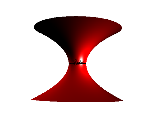
Figure 1: The Riemannian surface ${\cal S}$ of Eq. (161).

The “Schwarzschild wormhole” provides a path from the upper “universe” ${\cal S}_{+}$ ($Z>0$) to the lower one ${\cal S}_{-}$ ($Z<0$). These are both multiply connected surfaces. We will study the OCP on a single universe, on the whole surface, and on a single universe with the “horizon” (the region $r=2M$) grounded.

Since the curvature of the surface is not a constant but varies from point to point, the plasma will not be uniform even in the thermodynamic limit.

The system of coordinates $(r,\varphi)$ with the metric (160) has the disadvantage that it requires two charts to cover the whole surface ${\cal S}$. It can be more convenient to use the variable

$$u=\frac{Z}{4M}=\pm\sqrt{\frac{r}{2M}-1}$$ (162)

instead of $r$. Replacing $r$ as a function of $Z$ using equation (161) gives the following metric when using the system of coordinates $\mathbf{q}=(u,\varphi)$,

$$\mathbf{g}=\left(\begin{array}[]{cc}(4M)^{2}(1+u^{2})&0\\ 0&4M^{2}(1+u^{2})^{2}\end{array}\right),$$ (165)

The region $u>0$ corresponds to ${\cal S}_{+}$ and the region $u<0$ to ${\cal S}_{-}$.

Let us consider that the OCP is confined in a disk defined as

$$\Omega_{R}^{+}=\{\mathbf{q}=(r,\varphi)\in{\cal S}_{+}|0\leq\varphi\leq 2\pi,2M\leq r\leq R\}~{}.$$ (166)

The area of this disk is given by

$$\mathcal{A}_{R}=\int_{\Omega_{R}}dS=\pi\left[\sqrt{R(R-2M)}(3M+R)+6M^{2}\ln\left(\frac{\sqrt{R}+\sqrt{R-2M}}{\sqrt{2M}}\right)\right]~{},$$ (167)

where $dS=\sqrt{g}\,dr\,d\varphi$ and $g=\mathop{\mathrm{det}}[g_{\mu\nu}]$. The perimeter is $\mathcal{C}_{R}=2\pi R$.

The Riemann tensor characteristic component is

$${R^{r}}_{\varphi r\varphi}=-\frac{M}{r}~{}.$$ (168)

The scalar curvature is then given by the following indexes contractions

$$\mathcal{R}={R^{\mu}}_{\mu}={R^{\mu\nu}}_{\mu\nu}=2{R^{r\varphi}}_{r\varphi}=2g^{\varphi\varphi}{R^{r}}_{\varphi r\varphi}=-\frac{2M}{r^{3}}~{},$$ (169)

and the (intrinsic) Gaussian curvature is $K=\mathcal{R}/2=-M/r^{3}$. The (extrinsic) mean curvature of the manifold turns out to be $H=-\sqrt{M/8r^{3}}$.

The Euler characteristic (5) of the disk $\Omega_{R}^{+}$ turns out to be $\chi=0$, in agreement with the Gauss-Bonnet theorem $\chi=2-2h-b$ where $h=0$ is the number of handles and $b=2$ the number of boundaries.

We can also consider the case where the system is confined in a “double” disk

$$\Omega_{R}=\Omega_{R}^{+}\cup\Omega_{R}^{-}\,,$$ (170)

with $\Omega_{R}^{-}=\{\mathbf{q}=(r,\varphi)\in{\cal S}_{-}|0\leq\varphi\leq 2\pi,2M\leq r\leq R\}$, the disk image of $\Omega_{R}^{+}$ on the lower universe ${\cal S}_{-}$ portion of ${\cal S}$. The Euler characteristic of $\Omega_{R}$ is also $\chi=0$.

The fact that the Euler characteristic is zero implies that the asymptotic expansion in the thermodynamic limit of the free energy does not exhibit the logarithmic corrections predicted by Ref. Jancovici et al. (1994).

The Laplacian for a function $f$ is

$$\Delta f = \frac{1}{\sqrt{g}}\frac{\partial}{\partial q^{\mu}}\left(\sqrt{g}\,g^{\mu\nu}\frac{\partial}{\partial q^{\nu}}\right)f$$ (171)

$$= \left[\left(1-\frac{2M}{r}\right)\frac{\partial^{2}}{\partial r^{2}}+\frac{1}{r^{2}}\frac{\partial^{2}}{\partial\varphi^{2}}+\left(\frac{1}{r}-\frac{M}{r^{2}}\right)\frac{\partial}{\partial r}\right]f~{},$$

where $\mathbf{q}\equiv(r,\varphi)$. In appendix C, we show how, finding the Green function of the Laplacian, naturally leads to consider the system of coordinates $(x,\varphi)$, with

$$x=(\sqrt{u^{2}+1}+u)^{2}\,.$$ (172)

The range for the variable $x$ is $\left]0,+\infty\right[$. The lower paraboloid ${\cal S}_{-}$ corresponds to the region $0<x<1$ and the upper one ${\cal S}_{+}$ to the region $x>1$. A point in the upper paraboloid with coordinate $(x,\varphi)$ has a mirror image by reflection ($u\to-u$) in the lower paraboloid, with coordinates $(1/x,\varphi)$, since if

$$x=(\sqrt{u^{2}+1}+u)^{2}$$ (173)

then

$$\frac{1}{x}=(\sqrt{u^{2}+1}-u)^{2}\,.$$ (174)

In the upper paraboloid ${\cal S}_{+}$, the new coordinate $x$ can be expressed in terms of the original one, $r$, as

$$x=\frac{(\sqrt{r}+\sqrt{r-2M})^{2}}{2M}\,.$$ (175)

Using this system of coordinates, the metric takes the form of a flat metric multiplied by a conformal factor

$$\mathbf{g}=\left(\begin{array}[]{cc}(M/2)^{2}(1+1/x)^{4}&0\\ 0&(M/2)^{2}(1+1/x)^{4}x^{2}\end{array}\right),$$ (176)

The Laplacian also takes a simple form

$$\Delta f=\frac{4}{M^{2}\left(1+\frac{1}{x}\right)^{4}}\,\Delta_{\mathrm{flat}}f$$ (177)

where

$$\Delta_{\mathrm{flat}}f=\frac{\partial^{2}f}{\partial x^{2}}+\frac{1}{x}\frac{\partial f}{\partial x}+\frac{1}{x^{2}}\frac{\partial^{2}f}{\partial\varphi^{2}}$$ (178)

is the Laplacian of the flat Euclidean space $\mathbb{R}^{2}$. The determinant of the metric is now given by $g=[M^{2}x(1+x^{-1})^{4}/4]^{2}$.

With this system of coordinates $(x,\varphi)$, the area of a disk $\Omega_{R}^{+}$ of radius $R$, in the original system $(r,\varphi)$, is given by

$$\mathcal{A}_{R}=\frac{\pi M^{2}}{4}\,p(x_{m})$$ (179)

with

$$p(x)=x^{2}+8x-\frac{8}{x}-\frac{1}{x^{2}}+12\ln x$$ (180)

and $x_{m}=(\sqrt{R}+\sqrt{R-2M})^{2}/(2M)$.

The Coulomb potential $G(x,\varphi;x_{0},\varphi_{0})$ created at $(x,\varphi)$ by a unit charge at $(x_{0},\varphi_{0})$ is given by the Green function of the Laplacian

$$\Delta G(x,\varphi;x_{0},\varphi_{0})=-2\pi\delta^{(2)}(x,\varphi;x_{0},\varphi_{0})$$ (181)

with appropriate boundary conditions. The Dirac distribution on ${\cal S}$ is given by

$$\delta^{(2)}(x,\varphi;x_{0},\varphi_{0})=\frac{4}{M^{2}x(1+x^{-1})^{4}}\,\delta(x-x_{0})\delta(\varphi-\varphi_{0})$$ (182)

Notice that using the system of coordinates $(x,\varphi)$ the Laplacian Green function equation takes the simple form

$$\Delta_{\mathrm{flat}}G(x,\varphi;x_{0},\varphi_{0})=-2\pi\frac{1}{x}\,\delta(x-x_{0})\delta(\varphi-\varphi_{0})$$ (183)

which is formally the same Laplacian Green function equation for flat space.

We shall consider three different situations: when the particles can be in the whole surface ${\cal S}$, or when the particles are confined to the upper paraboloid universe ${\cal S}_{+}$, confined by a hard wall or by a grounded perfect conductor.

The geodesic distance on the Flamm paraboloid is determined in appendix D.

X.1 Coulomb potential in the whole surface (ws)

To complement the Laplacian Green function equation (181), we impose the usual boundary condition that the electric field $-\nabla G$ vanishes at infinity ($x\to\infty$ or $x\to 0$). Also, we require the usual interchange symmetry $G(x,\varphi;x_{0},\varphi_{0})=G(x_{0},\varphi_{0};x,\varphi)$ to be satisfied. Additionally, due to the symmetry between each universe ${\cal S}_{+}$ and ${\cal S}_{-}$, we require that the Green function satisfies the symmetry relation

$$G^{\mathrm{ws}}(x,\varphi;x_{0},\varphi_{0})=G^{\mathrm{ws}}(1/x,\varphi;1/x_{0},\varphi_{0})$$ (184)

The Laplacian Green function equation (181) can be solved, as usual, by using the decomposition as a Fourier series, as shown in appendix C. Since equation (181) reduces to the flat Laplacian Green function equation (183), the solution is the standard one

$$G(x,\varphi;x_{0},\varphi_{0})=\sum_{n=1}^{\infty}\frac{1}{n}\left(\frac{x_{<}}{x_{>}}\right)^{n}\cos\left[n(\varphi-\varphi_{0})\right]+g_{0}(x,x_{0})$$ (185)

where $x_{>}=\max(x,x_{0})$ and $x_{<}=\min(x,x_{0})$. The Fourier coefficient for $n=0$, has the form

$$g_{0}(x,x_{0})=\begin{cases}a_{0}^{+}\ln x+b_{0}^{+}\,,&x>x_{0}\\ a_{0}^{-}\ln x+b_{0}^{-}\,,&x<x_{0}\,.\end{cases}$$ (186)

The coefficients $a_{0}^{\pm},b_{0}^{\pm}$ are determined by the boundary conditions that $g_{0}$ should be continuous at $x=x_{0}$, its derivative discontinuous $\partial_{x}g_{0}|_{x=x_{0}^{+}}-\partial_{x}g_{0}|_{x=x_{0}^{-}}=-1/x_{0}$, and the boundary condition at infinity $\nabla g_{0}|_{x\to\infty}=0$ and $\nabla g_{0}|_{x\to 0}=0$. Unfortunately, the boundary condition at infinity is trivially satisfied for $g_{0}$, therefore $g_{0}$ cannot be determined only with this condition. In flat space, this is the reason why the Coulomb potential can have an arbitrary additive constant added to it. However, in our present case, we have the additional symmetry relation (184) which should be satisfied. This fixes the Coulomb potential up to an additive constant $b_{0}$. We find

$$g_{0}(x,x_{0})=-\frac{1}{2}\ln\frac{x_{>}}{x_{<}}+b_{0}\,,$$ (187)

and summing explicitly the Fourier series (185), we obtain

$$G^{\mathrm{ws}}(x,\varphi;x_{0},\varphi_{0})=-\ln\frac{\left|z-z_{0}\right|}{\sqrt{\left|zz_{0}\right|}}+b_{0}~{},$$ (188)

where we defined $z=xe^{i\varphi}$ and $z_{0}=x_{0}e^{i\varphi_{0}}$. Notice that this potential does not reduce exactly to the flat one when $M=0$. This is due to the fact that the whole surface $\mathcal{S}$ in the limit $M\to 0$ is not exactly a flat plane $\mathbb{R}^{2}$, but rather it is two flat planes connected by a hole at the origin, this hole modifies the Coulomb potential.

X.2 Coulomb potential in the half surface (hs) confined by hard walls

We consider now the case when the particles are restricted to live in the half surface ${\cal S}_{+}$, $x>1$, and they are confined by a hard wall located at the “horizon” $x=1$. The region $x<1$ (${\cal S}_{-}$) is empty and has the same dielectric constant as the upper region occupied by the particles. Since there are no image charges, the Coulomb potential is the same $G^{\mathrm{ws}}$ as above. However, we would like to consider here a new model with a slightly different interaction potential between the particles. Since we are dealing only with half surface, we can relax the symmetry condition (184). Instead, we would like to consider a model where the interaction potential reduces to the flat Coulomb potential in the limit $M\to 0$. The solution of the Laplacian Green function equation is given in Fourier series by equation (185). The zeroth order Fourier component $g_{0}$ can be determined by the requirement that, in the limit $M\to 0$, the solution reduces to the flat Coulomb potential

$$G^{\mathrm{flat}}(\mathbf{r},\mathbf{r}^{\prime})=-\ln\frac{|\mathbf{r}-\mathbf{r}^{\prime}|}{L}$$ (189)

where $L$ is an arbitrary constant length. Recalling that $x\sim 2r/M$, when $M\to 0$, we find

$$g_{0}(x,x_{0})=-\ln x_{>}-\ln\frac{M}{2L}$$ (190)

and

$$G^{\mathrm{hs}}(x,\varphi;x_{0},\varphi_{0})=-\ln|z-z_{0}|-\ln\frac{M}{2L}\,.$$ (191)

X.3 Coulomb potential on half surface with a grounded horizon (gh)

Let us consider now that the particles are confined to ${\cal S}_{+}$ by a grounded perfect conductor at $x=1$ which imposes Dirichlet boundary condition to the electric potential. The Coulomb potential can easily (see appendix C) be found from the Coulomb potential $G^{\mathrm{ws}}$ (188) using the method of images

$$G^{\mathrm{gh}}(x,\varphi;x_{0},\varphi_{0})=-\ln\frac{|z-z_{0}|}{\sqrt{|zz_{0}|}}+\ln\frac{|z-\bar{z}_{0}^{-1}|}{\sqrt{|z\bar{z}_{0}^{-1}|}}=-\ln\left|\frac{z-z_{0}}{1-z\bar{z}_{0}}\right|$$ (192)

where the bar over a complex number indicates its complex conjugate. We will call this the grounded horizon Green function. Notice how its shape is the same of the Coulomb potential on the pseudosphere Fantoni et al. (2003) or in a flat disk confined by perfect conductor boundaries Jancovici and Téllez (1996).

This potential can also be found using the Fourier decomposition. Since it will be useful in the following, we note that the zeroth order Fourier component of $G^{\mathrm{gh}}$ is

$$g_{0}(x,x_{0})=\ln x_{<}\,.$$ (193)

X.4 The background

The Coulomb potential generated by the background, with a constant surface charge density $\rho_{b}$ satisfies the Poisson equation, for $r>2M$,

$$\Delta v_{b}=-2\pi\rho_{b}~{},$$ (194)

Assuming that the system occupies an area $\mathcal{A}_{R}$, the background density can be written as $\rho_{b}=-qN_{b}/\mathcal{A}_{R}=-qn_{b}$, where we have defined here $n_{b}=N_{b}/\mathcal{A}_{R}$ the number density associated to the background. For a neutral system $N_{b}=N$. The Coulomb potential of the background can be obtained by solving Poisson equation with the appropriate boundary conditions for each case. Also, it can be obtained from the Green function computed in the previous section

$$v_{b}(x,\varphi)=\int G(x,\varphi;x^{\prime},\varphi^{\prime})\rho_{b}\,dS^{\prime}$$ (195)

This integral can be performed easily by using the Fourier series decomposition (185) of the Green function $G$. Recalling that $dS=\frac{1}{4}M^{2}x(1+x^{-1})^{4}\,dx\,d\varphi$, after the angular integration is done, only the zeroth order term in the Fourier series survives

$$v_{b}(x,\varphi)=\frac{\pi\rho_{b}M^{2}}{2}\int_{1}^{x_{m}}g_{0}(x,x^{\prime})\,x^{\prime}\left(1+\frac{1}{x^{\prime}}\right)^{4}\,dx^{\prime}\,.$$ (196)

The previous expression is for the half surface case and the grounded horizon case. For the whole surface case, the lower limit of integration should be replaced by $1/x_{m}$, or, equivalently, the integral multiplied by a factor two.

Using the explicit expressions for $g_{0}$, (187), (190), and (193) for each case, we find, for the whole surface,

$$v_{b}^{\mathrm{ws}}(x,\varphi)=-\frac{\pi\rho_{b}M^{2}}{8}\left[h(x)-h(x_{m})+2p(x_{m})\ln x_{m}-4b_{0}p(x_{m})\right]$$ (197)

where $p(x)$ was defined in equation (180), and

$$h(x)=x^{2}+16x+\frac{16}{x}+\frac{1}{x^{2}}+12(\ln x)^{2}-34\,.$$ (198)

Notice the following properties satisfied by the functions $p$ and $h$

$$p(x)=-p(1/x)\,,\qquad h(x)=h(1/x)$$ (199)

and

$$p(x)=xh^{\prime}(x)/2\,,\qquad p^{\prime}(x)=2x\left(1+\frac{1}{x}\right)^{4}$$ (200)

where the prime stands for the derivative.

The background potential for the half surface case, with the pair potential $-\ln(|z-z^{\prime}|M/2L)$ is

$$v_{b}^{\mathrm{hs}}(x,\varphi)=-\frac{\pi\rho_{b}M^{2}}{8}\left[h(x)-h(x_{m})+2p(x_{m})\ln\frac{x_{m}M}{2L}\right]\,.$$ (201)

Also, the background potential in the half surface case, but with the pair potential $-\ln(|z-z^{\prime}|/\sqrt{|zz^{\prime}|})+b_{0}$ is

$$v_{b}^{\overline{\mathrm{hs}}}(x,\varphi)=-\frac{\pi\rho_{b}M^{2}}{8}\left[h(x)-\frac{h(x_{m})}{2}+p(x_{m})\left(\ln\frac{x_{m}}{x}-2b_{0}\right)\right]\,.$$ (202)

Finally, for the grounded horizon case,

$$v_{b}^{\mathrm{gh}}(x,\varphi)=-\frac{\pi\rho_{b}M^{2}}{8}\left[h(x)-2p(x_{m})\ln x\right]\,.$$ (203)

X.5 Partition function and densities at a special temperature

We will now show how at the special value of the coupling constant $\Gamma=\beta e^{2}=2$ the partition function and $n$-body correlation functions can be calculated exactly.

X.5.1 The 2D OCP on half surface with potential $-\ln|z-z^{\prime}|-\ln M/(2L)$

For this case, we work in the canonical ensemble with $N$ particles and the background neutralizes the charges: $N_{b}=N$, and $n=N/\mathcal{A}_{R}=n_{b}$. The potential energy of the system takes the explicit form

$$V^{\mathrm{hs}} = -e^{2}\sum_{1\leq i<j\leq N}\ln|z_{i}-z_{j}|+\frac{e^{2}}{2}\alpha\sum_{i=1}^{N}h(x_{i})+\frac{e^{2}}{2}N\ln\frac{M}{2L}-\frac{e^{2}}{4}N\alpha h(x_{m})$$ (204)

$$+\frac{e^{2}}{2}N^{2}\ln x_{m}-\frac{e^{2}}{4}\alpha^{2}\int_{1}^{x_{m}}h(x)p^{\prime}(x)\,dx$$

where we have used the fact that $dS=\pi M^{2}x(1+x^{-1})^{4}\,dx/2=\pi M^{2}p^{\prime}(x)\,dx/4$, and we have defined

$$\alpha=\frac{\pi n_{b}M^{2}}{4}\,.$$ (205)

Integrating by parts the last term of (204) and using (200), we find

$$V^{\mathrm{hs}} = -e^{2}\sum_{1\leq i<j\leq N}\ln|z_{i}-z_{j}|+\frac{e^{2}}{2}\alpha\sum_{i=1}^{N}h(x_{i})+\frac{e^{2}}{2}N\ln\frac{M}{2L}+\frac{e^{2}}{2}N^{2}\ln x_{m}$$ (206)

$$+\frac{e^{2}}{2}\alpha^{2}\int_{1}^{x_{m}}\frac{[p(x)]^{2}}{x}\,dx-\frac{e^{2}}{2}N\alpha h(x_{m})\,.$$

When $\beta e^{2}=2$, the canonical partition function can be written as

$$Z^{\mathrm{hs}}=\frac{1}{\Lambda^{2N}}\,Z_{0}^{\mathrm{hs}}\exp(-\beta F_{0}^{\mathrm{hs}})$$ (207)

with

$$-\beta F_{0}^{\mathrm{hs}}=-N\ln\frac{M}{2L}-N^{2}\ln x_{m}-\alpha^{2}\int_{1}^{x_{m}}\frac{[p(x)]^{2}}{x}\,dx+N\alpha h(x_{m})$$ (208)

and

$$Z_{0}^{\mathrm{hs}}(2)=\frac{1}{N!}\int\prod_{i=1}^{N}dS_{i}\,e^{-\alpha h(x_{i})}\prod_{1\leq i<j\leq N}|z_{i}-z_{j}|^{2}\,.$$ (209)

where $\Lambda=\sqrt{2\pi\beta\hbar^{2}/m}$ is the de Broglie thermal wavelength. $Z_{0}(2)$ can be computed using the original method for the OCP in flat space Jancovici (1981a); Alastuey and Jancovici (1981), which was originally introduced in the context of random matrices Mehta (1991); Ginibre (1965), and which was presented in section VI. By expanding the van der Monde determinant $\prod_{i<j}(z_{i}-z_{j})$ and performing the integration over the angles, the partition function can be written as

$$Z_{0}^{\mathrm{hs}}(2) = \prod_{k=0}^{N-1}{\cal B}_{N}(k)~{},$$ (210)

where

$${\cal B}_{N}(k) = \int x^{2k}e^{-\alpha h(x)}\,dS$$ (211)

$$= \frac{\alpha}{n_{b}}\int_{1}^{x_{m}}x^{2k}e^{-\alpha h(x)}p^{\prime}(x)\,dx\,.$$ (212)

In the flat limit $M\to 0$, we have $x\sim 2r/M$, with $r$ the radial coordinate of flat space $\mathbb{R}^{2}$, and $h(x)\sim p(x)\sim x^{2}$. Then, $\mathcal{B}_{N}$ reduces to

$$\mathcal{B}_{N}(k)\sim\frac{1}{n_{b}\alpha^{k}}\,\gamma(k+1,N)$$ (213)

where $\gamma(k+1,N)=\int_{0}^{N}t^{k}e^{-t}\,dt$ is the incomplete Gamma function. Replacing into (210), we recover the partition function (29) for the OCP in a flat disk of radius $R$ Alastuey and Jancovici (1981)

$$\ln Z^{\mathrm{hs}}(2)=\frac{N}{2}\ln\frac{\pi L^{2}}{n_{b}\Lambda^{4}}+\frac{3N^{2}}{4}-\frac{N^{2}}{2}\ln N+\sum_{k=1}^{N}\ln\gamma(k,N)\,.$$ (214)

Following Jancovici (1981a), we can also find the $k$-body distribution functions

$$n^{(k){\mathrm{hs}}}(\mathbf{q}_{1},\ldots,\mathbf{q}_{k})=\mathop{\mathrm{det}}[{\cal K}_{N}^{\mathrm{hs}}(\mathbf{q}_{i},\mathbf{q}_{j})]_{(i,j)\in\{1,\ldots,k\}^{2}}~{},$$ (215)

where $\mathbf{q}_{i}=(x_{i},\varphi_{i})$ is the position of the particle $i$, and

$${\cal K}_{N}^{\mathrm{hs}}(\mathbf{q}_{i},\mathbf{q}_{j})=\sum_{k=0}^{N-1}\frac{z_{i}^{k}\bar{z}_{j}^{k}e^{-\alpha[h(|z_{i}|)+h(|z_{j}|)]/2}}{{\cal B}_{N}(k)}~{}.$$ (216)

where $z_{k}=x_{k}e^{i\varphi_{k}}$. In particular, the one-body density is given by

$$n^{\mathrm{hs}}(x)=\mathcal{K}_{N}(\mathbf{q},\mathbf{q})=\sum_{k=0}^{N-1}\frac{x^{2k}e^{-\alpha h(x)}}{\mathcal{B}_{N}(k)}\,.$$ (217)

The density shows a peak in the neighborhoods of each boundary, tends to a finite value at the boundary and to the background density far from it, in the bulk. This is shown in Fig. 2

Figure 2: The one body density $n^{\mathrm{hs}}(r)/n$ of Eq. (217), for the 2D OCP on just one universe of the surface ${\cal S}$, obtained with $N=300$. On the left at fixed $M=1$ and on the right at fixed $n=1$.

X.5.2 Internal screening

Internal screening means that at equilibrium, a particle of the system is surrounded by a polarization cloud of opposite charge. It is usually expressed in terms of the simplest of the multipolar sum rules Martin (1988): the charge or electroneutrality sum rule, which for the OCP reduces to the relation

$$\int n^{(2){\mathrm{hs}}}(\mathbf{q}_{1},\mathbf{q}_{2})\,dS_{2}=(N-1)n^{(1){\mathrm{hs}}}(\mathbf{q}_{1})~{},$$ (218)

This relation is trivially satisfied because of the particular structure (215) of the correlation function expressed as a determinant of the kernel $\mathcal{K}_{N}^{\mathrm{hs}}$, and the fact that $\mathcal{K}_{N}^{\mathrm{hs}}$ is a projector

$$\int dS_{3}\,\mathcal{K}_{N}^{\mathrm{hs}}(\mathbf{q}_{1},\mathbf{q}_{3})\mathcal{K}_{N}^{\mathrm{hs}}(\mathbf{q}_{3},\mathbf{q}_{2})=\mathcal{K}_{N}^{\mathrm{hs}}(\mathbf{q}_{1},\mathbf{q}_{2})\,.$$ (219)

Indeed,

$$\int n^{(2){\mathrm{hs}}}(\mathbf{q}_{1},\mathbf{q}_{2})\,dS_{2} = \int[{\cal K}_{N}^{\mathrm{hs}}(\mathbf{q}_{1},\mathbf{q}_{1}){\cal K}_{N}^{\mathrm{hs}}(\mathbf{q}_{2},\mathbf{q}_{2})-{\cal K}_{N}^{\mathrm{hs}}(\mathbf{q}_{1},\mathbf{q}_{2}){\cal K}_{N}^{\mathrm{hs}}(\mathbf{q}_{2},\mathbf{q}_{1})]\,dS_{2}$$ (220)

$$= \int n^{(1){\mathrm{hs}}}(\mathbf{q}_{1})n^{(1){\mathrm{hs}}}(\mathbf{q}_{2})\,dS_{2}-{\cal K}_{N}^{\mathrm{hs}}(\mathbf{q}_{1},\mathbf{q}_{1})$$

$$= (N-1)n^{(1){\mathrm{hs}}}(\mathbf{q}_{1})\,.$$

X.5.3 External screening

External screening means that, at equilibrium, an external charge introduced into the system is surrounded by a polarization cloud of opposite charge. When an external infinitesimal point charge $Q$ is added to the system, it induces a charge density $\rho_{Q}(\mathbf{q})$. External screening means that

$$\int\rho_{Q}(\mathbf{q})\,dS=-Q~{}.$$ (221)

Using linear response theory we can calculate $\rho_{Q}$ to first order in $Q$ as follows. Imagine that the charge $Q$ is at $\mathbf{q}$. Its interaction energy with the system is $\hat{H}_{int}=Q\hat{\phi}(\mathbf{q})$ where $\hat{\phi}(\mathbf{q})$ is the microscopic electric potential created at $\mathbf{q}$ by the system. Then, the induced charge density at $\mathbf{q}^{\prime}$ is

$$\rho_{Q}(\mathbf{q}^{\prime})=-\beta\langle\hat{\rho}(\mathbf{q}^{\prime})\hat{H}_{int}\rangle_{T}=-\beta Q\langle\hat{\rho}(\mathbf{q}^{\prime})\hat{\phi}(\mathbf{q})\rangle_{T}~{},$$ (222)

where $\hat{\rho}(\mathbf{q}^{\prime})$ is the microscopic charge density at $\mathbf{q}^{\prime}$, $\langle AB\rangle_{T}=\langle AB\rangle-\langle A\rangle\langle B\rangle$, and $\langle\ldots\rangle$ is the thermal average. Assuming external screening (221) is satisfied, one obtains the Carnie-Chan sum rule Martin (1988)

$$\beta\int\langle\hat{\rho}(\mathbf{q}^{\prime})\hat{\phi}(\mathbf{q})\rangle_{T}\,dS^{\prime}=1~{}.$$ (223)

Now in a uniform system starting from this sum rule one can derive the second moment Stillinger-Lovett sum rule Martin (1988). This is not possible here because our system is not homogeneous since the curvature is not constant throughout the surface but varies from point to point. If we apply the Laplacian respect to $\mathbf{q}$ to this expression and use Poisson equation

$$\Delta_{\mathbf{q}}\langle\hat{\rho}(\mathbf{q}^{\prime})\hat{\phi}(\mathbf{q})\rangle_{T}=-2\pi\langle\hat{\rho}(\mathbf{q}^{\prime})\hat{\rho}(\mathbf{q})\rangle_{T}~{},$$ (224)

we find

$$\int\rho_{e}^{(2)}(\mathbf{q}^{\prime},\mathbf{q})\,dS^{\prime}=0~{},$$ (225)

where $\rho_{e}^{(2)}(\mathbf{q}^{\prime},\mathbf{q})=\langle\hat{\rho}(\mathbf{q}^{\prime})\hat{\rho}(\mathbf{q})\rangle_{T}$ is the excess pair charge density function. Eq. (225) is another way of writing the charge sum rule Eq. (218) in the thermodynamic limit.

X.5.4 The 2D OCP on the whole surface with potential $-\ln(|z-z^{\prime}|/\sqrt{|zz^{\prime}|})$

Until now we studied the 2D OCP on just one universe. Let us find the thermodynamic properties of the 2D OCP on the whole surface ${\cal S}$. In this case, we also work in the canonical ensemble with a global neutral system. The position $z_{k}=x_{k}e^{i\varphi_{k}}$ of each particle can be in the range $1/x_{m}<x_{k}<x_{m}$. The total number particles $N$ is now expressed in terms of the function $p$ as $N=2\alpha p(x_{m})$. Similar calculations to the ones of the previous section lead to the following expression for the partition function, when $\beta e^{2}=2$,

$$Z^{\mathrm{ws}}=\frac{1}{\Lambda^{2N}}Z_{0}^{\mathrm{ws}}\exp(-\beta F_{0}^{\mathrm{ws}})$$ (226)

now, with

$$-\beta F_{0}^{\mathrm{ws}}=Nb_{0}+N\alpha h(x_{m})-\frac{N^{2}}{2}\ln x_{m}-\alpha^{2}\int_{1/x_{m}}^{x_{m}}\frac{\left[p(x)\right]^{2}}{x}\,dx$$ (227)

and

$$Z_{0}^{\mathrm{ws}}(2)=\frac{1}{N!}\int\prod_{i=1}^{N}dS_{i}\,e^{-\alpha h(x_{i})}x_{i}^{-N+1}\prod_{1\leq i<j\leq N}|z_{i}-z_{j}|^{2}\,.$$ (228)

Expanding the van der Monde determinant and performing the angular integrals we find

$$Z_{0}^{\mathrm{ws}}(2)=\prod_{k=0}^{N-1}\tilde{\mathcal{B}}_{N}(k)$$ (229)

with

$$\tilde{{\cal B}}_{N}(k) = \int x^{2k-N+1}e^{-\alpha h(x)}\,dS$$ (230)

$$= \frac{\alpha}{n}\int_{1/x_{m}}^{x_{m}}x^{2k-N+1}e^{-\alpha h(x)}p^{\prime}(x)\,dx\,.$$ (231)

The function $\tilde{\mathcal{B}}_{N}(k)$ is very similar to $\mathcal{B}_{N}$, and its asymptotic behavior for large values of $N$ can be obtained by Laplace method as explained in Ref. Fantoni and Téllez (2008).

The one body density for the 2D OCP on the whole manifold is drawn in Fig. 3. From the figure we can see how the peaks in the neighborhood of the horizon are now disappeared. The density approaches the horizon with zero slope.

Figure 3: The one body density $n^{(1)}(s)/n$, where $s=2Mx$, for the 2D OCP on the whole manifold, obtained using Eq. (231) with $N=300$. On the left at fixed $M=1$ and on the right at fixed $n=1$.

X.5.5 The 2D OCP on the half surface with potential $-\ln(|z-z^{\prime}|/\sqrt{|zz^{\prime}|})$

In this case, we have $N=\alpha p(x_{m})$. In this case the partition function at $\beta e^{2}=2$ is

$$Z^{\overline{\mathrm{hs}}}=Z_{0}^{\overline{\mathrm{hs}}}e^{-\beta F_{0}^{\overline{\mathrm{hs}}}}$$ (232)

with

$$-\beta F_{0}^{\overline{\mathrm{hs}}}=\alpha^{2}p(x_{m})h(x_{m})-p(x_{m})^{2}\ln x_{m}+\int_{1}^{x_{m}}\frac{\left[p(x)\right]^{2}}{x}\,dx-Nb_{0}$$ (233)

and

$$Z_{0}^{\overline{\mathrm{hs}}}(2)=\prod_{k=0}^{N-1}\hat{\mathcal{B}}_{N}(k)$$ (234)

with

$$\hat{\mathcal{B}}_{N}(k)=\frac{\alpha}{n_{b}}\int_{1}^{x_{m}}x^{2k+1}e^{-\alpha h(x)}\,dx$$ (235)

In Fig. 4 we compare the one body density obtained in this case with the one of the previous section.

Figure 4: The one body density $n^{(1)}(r)/n$, for the 2D OCP on just one universe of the surface ${\cal S}$, obtained using both the pair potential $-\ln|z-z^{\prime}|$ and $-\ln(|z-z^{\prime}|/\sqrt{|zz^{\prime}|})$ at fixed $M=n=1$.

X.5.6 The grounded horizon case

In order to find the partition function for the system in the half space, with a metallic grounded boundary at $x=1$, when the charges interact through the pair potential of Eq. (192) it is convenient to work in the grand canonical ensemble instead, and use the techniques developed in Refs. Forrester (1985); Jancovici and Téllez (1996). We consider a system with a fixed background density $\rho_{b}$. The fugacity $\zeta=e^{\beta\mu}/\Lambda^{2}$, where $\mu$ is the chemical potential, controls the average number of particles $\langle N\rangle$, and in general the system is non-neutral $\langle N\rangle\neq N_{b}$, where $N_{b}=\alpha p(x_{m})$. The excess charge is expected to be found near the boundaries at $x=1$ and $x=x_{m}$, while in the bulk the system is expected to be locally neutral. In order to avoid the collapse of a particle into the metallic boundary, due to its attraction to the image charges, we confine the particles to be in a disk domain $\tilde{\Omega}_{R}$, where $x\in[1+w,x_{m}]$. We introduced a small gap $w$ between the metallic boundary and the domain containing the particles, the geodesic width of this gap is $W=\sqrt{\alpha p^{\prime}(1)/(2\pi n_{b})}\,w$. On the other hand, for simplicity, we consider that the fixed background extends up to the metallic boundary.

In the potential energy of the system (9) we should add the self energy of each particle, that is due to the fact that each particle polarizes the metallic boundary, creating an induced surface charge density. This self energy is $\frac{e^{2}}{2}\ln[|x^{2}-1|M/2L]$, where the constant $\ln(M/2L)$ has been added to recover, in the limit $M\to 0$, the self energy of a charged particle near a plane grounded wall in flat space.

The grand partition function, when $\beta e^{2}=2$, is

$$\Xi(2)=e^{-\beta F_{0}^{\text{gh}}}\left[1+\sum_{N=1}^{\infty}\frac{\zeta^{N}}{N!}\int\prod_{i=1}^{N}dS_{i}\prod_{i<j}\left|\frac{z_{i}-z_{j}}{1-z_{i}\bar{z}_{j}}\right|^{2}\prod_{i=1}^{N}\left||z_{i}|^{2}-1\right|^{-1}\prod_{i=1}^{N}e^{-\alpha[h(x_{i})-2N_{b}\ln x_{i}]}\right]$$ (236)

where for $N=1$ the product $\prod_{i<j}$ must be replaced by 1. The domain of integration for each particle is $\tilde{\Omega}_{R}$. We have defined a rescaled fugacity $\zeta=2L\zeta/M$ and

$$-\beta F_{0}^{\text{gh}}=\alpha N_{b}h(x_{m})-N_{b}^{2}\ln x_{m}-\alpha^{2}\int_{1}^{x_{m}}\frac{[p(x)]^{2}}{x}\,dx$$ (237)

which is very similar to $F_{0}^{\text{hs}}$, except that here $N_{b}=\alpha p(x_{m})$ is not equal to $N$ the number of particles.

Let us define a set of reduced complex coordinates $u_{i}=z_{i}$ and its corresponding images $u_{i}^{*}=1/\bar{z}_{i}$. By using Cauchy identity (130),

$$\mathop{\mathrm{det}}\left(\frac{1}{u_{i}-u_{j}^{*}}\right)_{(i,j)\in\{1,\cdots,N\}^{2}}=(-1)^{N(N-1)/2}\>\frac{\prod_{i<j}(u_{i}-u_{j})(u^{*}_{i}-u^{*}_{j})}{\prod_{i,j}(u_{i}-u_{j}^{*})},$$ (238)

the particle-particle interaction and self energy terms can be cast into the form

$$\prod_{i<j}\left|\frac{z_{i}-z_{j}}{1-z_{i}\bar{z}_{j}}\right|^{2}\prod_{i=1}^{N}\left(|z_{i}|^{2}-1\right)^{-1}=(-1)^{N}\mathop{\mathrm{det}}\left(\frac{1}{1-z_{i}\bar{z}_{j}}\right)_{(i,j)\in\{1,\cdots,N\}^{2}}\,.$$ (239)

The grand canonical partition function is then

$$\Xi(2)=e^{-\beta F_{0}^{\text{gh}}}\left[1+\sum_{N=1}^{\infty}\frac{1}{N!}\int\prod_{i=1}^{N}dS_{i}\prod_{i=1}^{N}\left[-\zeta(x_{i})\right]\,\mathop{\mathrm{det}}\left(\frac{1}{1-z_{i}\bar{z}_{j}}\right)\right]\,,$$ (240)

with $\zeta(x)=\zeta e^{-\alpha[h(x)-2N_{b}\ln x]}$. We now notice that we already found an analogous expression (132) when studying the pseudosphere. We therefore proceed as we did for that case. For ease of reading we repeat here the relevant steps reducing this expression to a Fredholm determinant Forrester (1985). Then let us consider the Gaussian partition function

$$Z_{0}=\int{\cal D}\psi{\cal D}\bar{\psi}\,\exp\left[\int\bar{\psi}(\mathbf{q})A^{-1}(z,\bar{z}^{\prime})\psi(\mathbf{q}^{\prime})\,dS\,dS^{\prime}\right]$$ (241)

The fields $\psi$ and $\bar{\psi}$ are anticommuting Grassmann variables. The Gaussian measure in (241) is chosen such that its covariance is equal to

$$\left<\bar{\psi}(\mathbf{q}_{i})\psi(\mathbf{q}_{j})\right>=A(z_{i},\bar{z}_{j})=\frac{1}{1-z_{i}\bar{z}_{j}}$$ (242)

where $\langle\ldots\rangle$ denotes an average taken with the Gaussian weight of (241). By construction we have

$$Z_{0}=\mathop{\mathrm{det}}(A^{-1})$$ (243)

Let us now consider the following partition function

$$Z=\int{\cal D}\psi{\cal D}\bar{\psi}\exp\left[\int\bar{\psi}(\mathbf{q})A^{-1}(z,\bar{z}^{\prime})\psi(\mathbf{q}^{\prime})dSdS^{\prime}-\int\zeta(x)\bar{\psi}(\mathbf{q})\psi(\mathbf{q})\,dS\right]$$ (244)

which is equal to

$$Z=\mathop{\mathrm{det}}(A^{-1}-\zeta)$$ (245)

and then

$$\frac{Z}{Z_{0}}=\mathop{\mathrm{det}}[A(A^{-1}-\zeta)]=\mathop{\mathrm{det}}(1+K)$$ (246)

where $K$ is an integral operator (with integration measure $dS$) with kernel

$$K(\mathbf{q},\mathbf{q}^{\prime})=-\zeta(x^{\prime})\,A(z,\bar{z}^{\prime})=-\frac{\zeta(x^{\prime})}{1-z\bar{z}^{\prime}}\,.$$ (247)

Expanding the ratio $Z/Z_{0}$ in powers of $\zeta$ we have

$$\frac{Z}{Z_{0}}=1+\sum_{N=1}^{\infty}\frac{1}{N!}\int\prod_{i=1}^{N}dS_{i}(-1)^{N}\prod_{i=1}^{N}\zeta(x_{i})\left<\bar{\psi}(\mathbf{q}_{1})\psi(\mathbf{q}_{1})\cdots\bar{\psi}(\mathbf{q}_{N})\psi(\mathbf{q}_{N})\right>$$ (248)

Now, using Wick theorem for anticommuting variables Zinn-Justin (1993), we find that

$$\left<\bar{\psi}(\mathbf{q}_{1})\psi(\mathbf{q}_{1})\cdots\bar{\psi}(\mathbf{q}_{N})\psi(\mathbf{q}_{N})\right>=\mathop{\mathrm{det}}A(z_{i},\bar{z}_{j})=\mathop{\mathrm{det}}\left(\frac{1}{1-z_{i}\bar{z}_{j}}\right)$$ (249)

Comparing equations (248) and (240) with the help of equation (249) we conclude that

$$\Xi(2)=e^{-\beta F_{0}^{\text{gh}}}\,\frac{Z(2)}{Z_{0}(2)}=e^{-\beta F_{0}^{\text{gh}}}\mathop{\mathrm{det}}(1+K)$$ (250)

The problem of computing the grand canonical partition function has been reduced to finding the eigenvalues $\lambda$ of the operator $K$. The eigenvalue problem for $K$ reads

$$-\int_{\tilde{\Omega}_{R}}\frac{\zeta(x^{\prime})}{1-z\bar{z}^{\prime}}\,\Phi(x^{\prime},\varphi^{\prime})dS^{\prime}=\lambda\Phi(x,\varphi)$$ (251)

For $\lambda\neq 0$ we notice from equation (251) that $\Phi(x,\varphi)=\Phi(z)$ is an analytical function of $z=xe^{i\varphi}$ in the region $|z|>1$. Because of the circular symmetry, it is natural to try $\Phi(z)=\Phi_{\ell}(z)=z^{-\ell}$ with $\ell\geq 1$ a positive integer. Expanding

$$\frac{1}{1-z\bar{z}^{\prime}}=-\sum_{n=1}^{\infty}\left(z\bar{z}^{\prime}\right)^{-n}$$ (252)

and replacing $\Phi_{\ell}(z)=z^{-\ell}$ in equation (251) we show that $\Phi_{\ell}$ is indeed an eigenfunction of $K$ with eigenvalue

$$\lambda_{\ell}=\zeta\mathcal{B}_{N_{b}}^{\text{gh}}(N_{b}-\ell)$$ (253)

where

$$\mathcal{B}_{N_{b}}^{\text{gh}}(k)=\frac{\alpha}{n_{b}}\int_{1+w}^{x_{m}}x^{2k}e^{-\alpha h(x)}\,p^{\prime}(x)\,dx$$ (254)

which is very similar to $\mathcal{B}_{N}$ defined in Eq. (212), except for the small gap $w$ in the lower limit of integration. So, we arrive to the result for the grand potential

$$\beta\Omega=-\ln\Xi(2)=\beta F_{0}-\sum_{\ell=1}^{\infty}\ln\left[1+\zeta{\cal B}_{N_{b}}^{\text{gh}}(N_{b}-\ell)\right]\,.$$ (255)

As usual one can compute the density by doing a functional derivative of the grand potential with respect to a position-dependent fugacity $\zeta(\mathbf{q})$

$$n^{\text{gh}}(\mathbf{q})=\zeta(\mathbf{q})\frac{\delta\ln\Xi(2)}{\delta\zeta(\mathbf{q})}\,.$$ (256)

For the present case of a curved space, we shall understand the functional derivative with the rule $\delta\zeta(\mathbf{q}^{\prime})/\delta\zeta(\mathbf{q})=\delta^{(2)}(\mathbf{q};\mathbf{q}^{\prime})$ where $\delta^{(2)}(\mathbf{q};\mathbf{q}^{\prime})=\delta(x-x^{\prime})\delta(\varphi-\varphi^{\prime})/\sqrt{g}$ is the Dirac distribution on the curved surface.

Using a Dirac-like notation, one can formally write

$$\ln\Xi(2)=\mathop{\mathrm{tr}}\ln(1+K)-\beta F_{0}^{\text{gh}}=\int\left<\mathbf{q}\left|\ln(1-\zeta(\mathbf{q})A)\right|\mathbf{q}\right>\,dS-\beta F_{0}^{\text{gh}}$$ (257)

Then, doing the functional derivative (256), one obtains

$$n^{\text{gh}}(\mathbf{q})=\zeta\left<\mathbf{q}\left|(1+K)^{-1}(-A)\right|\mathbf{q}\right>=\zeta\tilde{G}(\mathbf{q},\mathbf{q})$$ (258)

where we have defined $\tilde{G}(\mathbf{q},\mathbf{q}^{\prime})$ by $\tilde{G}=(1+K)^{-1}(-A)$. More explicitly, $G$ is the solution of $(1+K)\tilde{G}=-A$, that is

$$\tilde{G}(\mathbf{q},\mathbf{q}^{\prime})-\int_{\tilde{\Omega}_{R}}\zeta(x^{\prime\prime})\frac{\tilde{G}(\mathbf{q}^{\prime\prime},\mathbf{q}^{\prime})}{1-z\bar{z}^{\prime\prime}}\,dS^{\prime\prime}=-\frac{1}{1-z\bar{z}^{\prime}}\,.$$ (259)

From this integral equation, one can see that $\tilde{G}(\mathbf{q},\mathbf{q}^{\prime})$ is an analytical function of $z$ in the region $|z|>1$. Then, we look for a solution in the form of a Laurent series

$$\tilde{G}(\mathbf{q},\mathbf{q}^{\prime})=\sum_{\ell=1}^{\infty}a_{\ell}(\mathbf{r}^{\prime})z^{-\ell}$$ (260)

into equation (259) yields

$$\tilde{G}(\mathbf{q},\mathbf{q}^{\prime})=\sum_{\ell=1}^{\infty}\frac{\left(z\bar{z}^{\prime}\right)^{-\ell}}{1+\lambda_{\ell}}\,.$$ (261)

Recalling that $\lambda_{\ell}=\zeta\mathcal{B}_{N}^{\text{gh}}(N_{b}-\ell)$, the density is given by

$$n^{\text{gh}}(x)=\zeta\sum_{k=-\infty}^{N_{b}-1}\frac{x^{2k}e^{-\alpha h(x)}}{1+\zeta\mathcal{B}_{N}^{\text{gh}}(k)}$$ (262)

The density reaches the background density far from the boundaries. In this case, the fugacity and the background density control the density profile close to the metallic boundary (horizon). In the bulk and close to the outer hard wall boundary, the density profile is independent of the fugacity. In Fig. 5 we show the density for various choices of the parameters $M,n$, and $\zeta$. The figure shows how the density tends to the background density far from the horizon. The value of the density at the horizon depends on $n$ and $\zeta$.

Figure 5: The one body density $n^{\text{gh}}(r)/n$ obtained truncating the sum of Eq. (262) after the first $300$ terms and choosing $(\sqrt{R}+\sqrt{R-2M})^{2}/2M=10$. On top on the left at fixed $M=\zeta=1$ and on the right at fixed $n=\zeta=1$. On the bottom at fixed $M=n=1$.

Part III The Two-Component Plasma

A two-component plasma is a neutral mixture of two species of $2N$ point charges of opposite charge $\pm e$.

XI The plane

We represent the Cartesian components of the position $\mathbf{q}=(x,y)$ of a particle by the complex number $z=x+iy$. For a system of $N$ positive charges with complex coordinates $u_{i}$ and $N$ negative charges with complex coordinates $v_{i}$ the Boltzmann factor at $\Gamma=\beta e^{2}=2$ is,

$$e^{2\sum_{i<j}\left[\ln\frac{|u_{i}-u_{j}|}{L}+\ln\frac{|v_{i}-v_{j}|}{L}\right]-2\sum_{i,j}\ln\frac{|u_{i}-v_{j}|}{L}} = L^{2N}\left|\frac{\prod_{i<j}(u_{i}-u_{j})(v_{i}-v_{j})}{\prod_{i,j}(u_{i}-v_{j})}\right|^{2}$$ (263)

$$= L^{2N}\left|\mathop{\mathrm{det}}\left(\frac{1}{u_{i}-v_{j}}\right)_{(i,j)\in\{1,\cdots,N\}^{2}}\right|^{2},$$

where the last equality stems from the Cauchy identity (130). Following Ref. Cornu and Jancovici (1987), it is convenient to start with a discretized model for which there are no divergencies. Two interwoven sublattices $U$ and $V$ are introduced. The positive (negative) particles sit on the sublattice $U(V)$. Each lattice site is occupied no or one particle. A possible external potential is described by position dependent fugacities $\zeta_{+}(u_{i})$ and $\zeta_{-}(v_{i})$. The the grand partition function reorganized as a sum including only neutral systems is

$$\Xi(2) = 1+\sum_{N=1}^{\infty}L^{2N}\prod_{i=1}^{N}\zeta_{+}(u_{i})\zeta_{-}(v_{i})\mathop{\sum_{u_{1},\ldots,u_{N}\in U}}_{v_{1},\ldots,v_{N}\in V}\left|\mathop{\mathrm{det}}\left(\frac{1}{u_{i}-v_{j}}\right)_{(i,j)\in\{1,\ldots,N\}^{2}}\right|^{2}~{},$$ (264)

where the sums are defined with the prescription that configurations which differ only by a permutation of identical particles are counted only once. This grand partition function is the determinant of an anti-Hermitian matrix $\mathbf{M}$ explicitly shown in Ref. Cornu and Jancovici (1989).

When passing to the continuum limit in the element $\mathbf{M}_{ij}$ one should replace $u_{i}$ or $v_{i}$ by $z$ and $u_{j}$ or $v_{j}$ by $z^{\prime}$, i.e. $i\to z$ and $j\to z^{\prime}$. Each lattice site is characterized by its complex coordinate $z$ and an isospinor which is $\left(\begin{array}[]{c}1\\ 0\end{array}\right)$ if the site belongs to the positive sublattice $U$ and $\left(\begin{array}[]{c}0\\ 1\end{array}\right)$ if it belongs to the negative sublattice $V$. We then define a matrix $\boldsymbol{\mathcal{M}}$ by

$$\langle z|\boldsymbol{\mathcal{M}}|z^{\prime}\rangle=\frac{\boldsymbol{\sigma_{x}}+i\boldsymbol{\sigma_{y}}}{2}\frac{L}{z-z^{\prime}}+\frac{\boldsymbol{\sigma_{x}}-i\boldsymbol{\sigma_{y}}}{2}\frac{L}{\overline{z}-\overline{z}^{\prime}}~{},$$ (265)

where the $\boldsymbol{\sigma}$ are the $2\times 2$ Pauli matrices operating in the isospinor space.

The matrix $\boldsymbol{\mathcal{M}}$ can be expressed in terms of a simple Dirac operator $\not{\partial}=\boldsymbol{\sigma_{x}}\partial_{x}+\boldsymbol{\sigma_{y}}\partial_{y}$ as follows,

$$\langle z|\boldsymbol{\mathcal{M}}|z^{\prime}\rangle=L(\boldsymbol{\sigma_{x}}\partial_{x}+\boldsymbol{\sigma_{y}}\partial_{y})\ln|z-z^{\prime}|~{},$$ (266)

and the grand partition function can be rewritten as

$$\Xi(2) = \mathop{\mathrm{det}}\left\{\mathbf{1}\delta^{(2)}(z;z^{\prime})+\left[\zeta_{+}(z)\frac{\mathbf{1}+\boldsymbol{\sigma_{z}}}{2}+\zeta_{-}(z)\frac{\mathbf{1}-\boldsymbol{\sigma_{z}}}{2}\right]\langle z|\boldsymbol{\mathcal{M}}|z^{\prime}\rangle\right\}$$ (267)

$$= \mathop{\mathrm{det}}[\mathbf{1}+\boldsymbol{\mathcal{K}}^{-1}]~{},$$

where $\mathbf{1}$ is the $2\times 2$ identity matrix and

$$\boldsymbol{\lambda} = \zeta_{+}\frac{\mathbf{1}+\boldsymbol{\sigma_{z}}}{2}+\zeta_{-}\frac{\mathbf{1}-\boldsymbol{\sigma_{z}}}{2}~{},$$ (268)

$$\boldsymbol{\mathcal{K}}^{-1} = \boldsymbol{\lambda}\boldsymbol{\mathcal{M}}~{}.$$ (269)

Then, since $\Delta\ln|z|=2\pi\delta(r)\delta(\varphi)/r=2\pi\delta(z)$, where $(r=|z|,\varphi=\arg z)$ are the polar coordinates in the plane, the inverse operator is $\boldsymbol{\mathcal{K}}=\boldsymbol{\mathcal{O}}\mathbf{m}^{-1}$, where

$$\mathbf{m}(z) = m_{+}(z)\frac{\mathbf{1}+\boldsymbol{\sigma_{z}}}{2}+m_{-}(z)\frac{\mathbf{1}-\boldsymbol{\sigma_{z}}}{2}~{},$$ (270)

$$\boldsymbol{\mathcal{O}} = \boldsymbol{\sigma_{x}}\partial_{x}+\boldsymbol{\sigma_{y}}\partial_{y}=\not{\partial}~{}.$$ (271)

Here $m_{\pm}(z)=2\pi L\zeta_{\pm}(z)/S$ are rescaled position dependent fugacities and $S$ is the area per lattice site which appears when the discrete sums are replaced by integrals.

We then find

$$\ln\Xi(2) = \mathop{\mathrm{tr}}\left\{\ln\left[\mathbf{1}+\boldsymbol{\mathcal{K}}^{-1}\right]\right\}~{},$$

which expresses the well known equivalence between the 2D OCP at $\Gamma=2$ and a free Fermi field Samuel (1978).

The one-body densities and $n$-body truncated densities Martin (1988) can be obtained in the usual way by taking functional derivatives of the logarithm of the grand partition function with respect to the fugacities $\zeta_{\pm}$. Marking the sign of the particle charge at $z_{i}$ by an index $p_{i}=\pm$, and defining the matrix

$$R_{p_{1}p_{2}}(z_{1},z_{2})=\langle z_{1}p_{1}|\boldsymbol{\mathcal{K}}^{-1}(1+\boldsymbol{\mathcal{K}}^{-1})^{-1}|z_{2}p_{2}\rangle~{},$$ (272)

it can then be shown Cornu and Jancovici (1987, 1989) that they are given by

$$\rho_{p_{1}}^{(1)}(z_{1}) = R_{p_{1}p_{1}}(z_{1},z_{1})~{},$$ (273)

$$\rho_{p_{1}p_{2}}^{(2)T}(z_{1},z_{2}) = -R_{p_{1}p_{2}}(z_{1},z_{2})R_{p_{2}p_{1}}(z_{2},z_{1})~{},$$ (274)

$$\rho_{p_{1}p_{2},\ldots,p_{n}}^{(n)T}(z_{1},z_{2},\ldots,z_{n}) = (-)^{n+1}\sum_{(i_{1},i_{2},\ldots,i_{n})}R_{p_{i_{1}}p_{i_{2}}}(z_{i_{1}},z_{i_{2}})\cdots R_{p_{i_{n}}p_{i_{1}}}(z_{i_{n}},z_{i_{1}})~{},$$ (275)

where the summation runs over all cycles $(i_{1},i_{2},\ldots,i_{n})$ built with $\{1,2,\ldots,n\}$.

XI.1 Symmetries of Green’s function $R$

Since $\mathbf{m}^{\dagger}=\mathbf{m}$ and $\boldsymbol{\mathcal{O}}^{\dagger}=-\boldsymbol{\mathcal{O}}$ we find

$$\overline{R_{p_{1}p_{2}}(z_{1},z_{2})}=\langle z_{2}p_{2}|\mathbf{m}(z)(\mathbf{m}(z)-\boldsymbol{\mathcal{O}})^{-1}|z_{1}p_{1}\rangle~{}.$$ (276)

Expanding in $\boldsymbol{\mathcal{O}}$ and comparing with the definition $R_{p_{1}p_{2}}(z_{1},z_{2})=\langle z_{1}p_{1}|\mathbf{m}(z)(\mathbf{m}(z)+\boldsymbol{\mathcal{O}})^{-1}|z_{2}p_{2}\rangle$ we find

$$\overline{R_{pp}(z_{1},z_{2})}=R_{pp}(z_{2},z_{1})~{},$$ (277)

$$\overline{R_{p-p}(z_{1},z_{2})}=-R_{-pp}(z_{2},z_{1})~{}.$$ (278)

From which also follows that $R_{pp}(z_{1},z_{1})$ has to be real. If $\zeta_{+}=\zeta_{-}$ then we additionally must have

$$R_{pp}(z_{1},z_{2})=R_{-p-p}(z_{1},z_{2})~{}.$$ (279)

XI.2 Two-body truncated correlation functions and perfect screening sum rule

For the two-body truncated correlation functions of Eq. (274) we then find

$$\rho_{++}^{(2)T}(z_{1},z_{2}) = -|R_{++}(z_{1},z_{2})|^{2}~{},$$ (280)

$$\rho_{+-}^{(2)T}(z_{1},z_{2}) = |R_{+-}(z_{1},z_{2})|^{2}~{}.$$ (281)

Notice that the total correlation function for the like particles $h_{++}(z_{1},z_{2})$ $=$ $\rho_{++}^{(2)T}(z_{1},z_{2})$ $/\rho_{+}^{(1)}(z_{1})\rho_{+}^{(1)}(z_{2})$ goes to $-1$ when the particles coincide $z_{1}\to z_{2}$ as follows from the structure of Eqs. (273) and (274). Moreover the truncated densities of any order has to decay to zero as two groups of particles are infinitely separated. In particular $|R_{++}(z_{1},z_{2})|=|R_{++}(r_{1},r_{2},\varphi_{2}-\varphi_{1})|$ has to decay to zero as $|\mathbf{q}_{1}-\mathbf{q}_{2}|\to\infty$.

The perfect screening sum rule has to be satisfied for the symmetric mixture

$$\int[\rho_{+-}^{(2)T}(z_{1},z_{2})-\rho^{(2)T}_{++}(z_{1},z_{2})]\sqrt{g_{1}}dr_{1}d\varphi_{1}=\rho_{\pm}(z_{2})~{},$$ (282)

where $g_{1}$ is $g$ calculated on particle 1.

XI.3 Determination of Green’s function $R$

The Green function matrix $\mathbf{R}$ is the solution of a system of four coupled partial differential equations, namely

$$(\mathbf{1}+\boldsymbol{\mathcal{K}}^{-1})\boldsymbol{\mathcal{K}}\mathbf{R}(z_{1},z_{2})=(\mathbf{1}+\boldsymbol{\mathcal{K}})\mathbf{R}(z_{1},z_{2})=\mathbf{1}\delta^{(2)}(z_{1};z_{2})$$ (283)

where $\delta^{(2)}(z_{1};z_{2})$ $=$ $(\sqrt{g})^{-1}\delta(r-r_{0})\delta(\varphi-\varphi_{0})$, with $\sqrt{g}=r$ is the Dirac delta function on the plane which we will call $\delta(z_{1}-z_{2})$ the flat Dirac delta and $\mathbf{1}$ is the $2\times 2$ identity matrix. These coupled equations can be rewritten as follows

$$\left[\boldsymbol{\mathcal{O}}+\mathbf{m}(z_{1})\right]\mathbf{R}(z_{1},z_{2})=\mathbf{m}(z_{1})\delta^{(2)}(z_{1};z_{2})~{}.$$

If instead of $\mathbf{R}$ one uses $\mathbf{R}=\mathbf{G}\mathbf{m}$, $\mathbf{G}$ satisfies the equation

$$[\boldsymbol{\mathcal{O}}+\mathbf{m}(z_{1})]\mathbf{G}(z_{1},z_{2})=\mathbf{1}\delta^{(2)}(z_{1};z_{2})~{}.$$ (284)

By combining the components of this equation one obtains decoupled equations for $G_{++}$ and $G_{--}$ as follows

$$\left\{m_{+}(z_{1})+A^{\dagger}[m_{-}(z_{1})]^{-1}A\right\}G_{++}(z_{1},z_{2}) = \delta^{(2)}(r_{1},\varphi_{1};r_{2},\varphi_{2})~{},$$ (285)

$$\left\{m_{-}(z_{1})+A[m_{+}(z_{1})]^{-1}A^{\dagger}\right\}G_{--}(z_{1},z_{2}) = \delta^{(2)}(r_{1},\varphi_{1};r_{2},\varphi_{2})~{},$$ (286)

where $A=\partial_{x}+i\partial_{y}$, while

$$G_{-+}(z_{1},z_{2}) = -\left[m_{-}(z_{1})\right]^{-1}AG_{++}(z_{1},z_{2})~{},$$ (287)

$$G_{+-}(z_{1},z_{2}) = +\left[m_{+}(z_{1})\right]^{-1}A^{\dagger}G_{--}(z_{1},z_{2})~{},$$ (288)

Then Eq. (318) can be rewritten in Cartesian coordinates as

$$\left[m_{+}m_{-}-\frac{1}{r_{1}}\partial_{r_{1}}(r_{1}\partial_{r_{1}})-\frac{1}{r_{1}^{2}}\partial^{2}_{\varphi_{1}}\right]G_{++}(z_{1},z_{2})=\frac{m_{-}}{r_{1}}\delta(r_{1}-r_{2})\delta(\varphi_{1}-\varphi_{2})~{}.$$ (289)

which, when $m_{+}(z)=m_{-}(z)=m$, has the following solution Cornu and Jancovici (1989, 1987)

$$G_{++}(z_{1},z_{2}) = \frac{m}{2\pi}K_{0}(m|\mathbf{q}_{1}-\mathbf{q}_{2}|)~{},$$ (290)

$$G_{-+}(z_{1},z_{2}) = \frac{m}{2\pi}\frac{(x_{1}-x_{2})+i(y_{1}-y_{2})}{|\mathbf{q}_{1}-\mathbf{q}_{2}|}K_{1}(m|\mathbf{q}_{1}-\mathbf{q}_{2}|)~{},$$ (291)

where $K_{0}$ and $K_{1}$ are modified Bessel functions. These functions decay at large distances on a characteristic length scale $m^{-1}$. The $n$-body truncated densities (275) are well defined quantities for the point particle system. The two-body truncated densities, for example, have the simple forms

$$\rho_{++}^{(2)T}(r) = -\left(\frac{m^{2}}{2\pi}\right)^{2}K_{0}^{2}(mr),$$ (292)

$$\rho_{+-}^{(2)T}(r) = -\left(\frac{m^{2}}{2\pi}\right)^{2}K_{1}^{2}(mr).$$ (293)

The one-body densities, however, as given by Eq. (273), are infinite since $K_{0}(mr)$ diverges logarithmically as $r\to 0$. This divergence can be suppressed by a short distance cutoff $R$. We replace the point particles by small hard discs of diameter $R$ and use a regularized form of Eq. (273),

$$\rho_{\pm}=\frac{m^{2}}{2\pi}K_{0}(mR)\sim\frac{m^{2}}{2\pi}\left[\ln\frac{2}{mR}-\gamma\right],$$ (294)

where $\gamma=0.5772$ is Euler’s constant. Keeping the point charge expression for the correlation functions for separations larger than $R$ the perfect screening rule (282) is satisfied.

Integrating $\rho_{+}+\rho_{-}=m\partial(\beta p)/\partial m$, from Eq. (294) one obtains for the pressure $p$,

$$\beta p=\frac{1}{2}(\rho_{+}+\rho_{-})+\frac{m^{2}}{4\pi}.$$ (295)

The same result can be obtained by using the regularized form of Eq. (267). In the limit $mR\to 0$ one finds the expected result for an ideal gas of collapsed neutral pairs.

XII The sphere

We consider the stereographic projection Forrester et al. (1992) of the sphere of radius $a$ on the plane tangent to its south pole. The coordinates of the point $\mathbf{p}=(x,y)$ stereographic projection of a point $\mathbf{q}=(\theta,\varphi)$ of the sphere from the north pole is given in terms of the complex coordinate $z=x+iy$ by $z=2ae^{i\varphi}\text{cotan}(\theta/2)$. This projection is a conformal transformation. The conformal metric in the new coordinates $(x,y)$ is then

$$\mathbf{g}=\left(\begin{array}[]{cc}e^{\omega}&0\\ 0&e^{\omega}\end{array}\right),$$ (298)

with the conformal factor given by

$$e^{\omega}=\sin^{2}\frac{\theta}{2}=\frac{1}{1+(|z|/2a)^{2}}.$$ (299)

The length $r_{ij}$ (52) of the chord joining two particles $i$ and $j$ has a simple relation with its projection $|z_{i}-z_{j}|$,

$$r_{ij}=e^{\omega_{i}/2}|z_{i}-z_{j}|e^{\omega_{j}/2}=\sin\frac{\theta_{i}}{2}|z_{i}-z_{j}|\sin\frac{\theta_{j}}{2}.$$ (300)

We can then follow the same steps as in section XI with $z-z^{\prime}$ replaced by $e^{\omega/2}(z-z^{\prime})e^{\omega^{\prime}/2}$. In particular the matrix $\boldsymbol{\mathcal{M}}$ will now become,

$$\langle z|\boldsymbol{\mathcal{M}}|z^{\prime}\rangle=\frac{\boldsymbol{\sigma_{x}}+i\boldsymbol{\sigma_{y}}}{2}\frac{L}{e^{\omega/2}(z-z^{\prime})e^{\omega^{\prime}/2}}+\frac{\boldsymbol{\sigma_{x}}-i\boldsymbol{\sigma_{y}}}{2}\frac{L}{e^{\omega/2}(\overline{z}-\overline{z}^{\prime})e^{\omega^{\prime}/2}}~{},$$ (301)

In the inverse operator $\boldsymbol{\mathcal{K}}$ we now have

$$\boldsymbol{\mathcal{O}}=e^{-3\omega/2}\not{\partial}e^{\omega/2}=\not{D},$$ (302)

since the Dirac delta function on the sphere $\delta^{(2)}(z;z^{\prime})=e^{-2\omega}\delta(z-z^{\prime})$ where $\delta$ is the flat Dirac delta function.

Thus, the Dirac operator $\not{\partial}$ in the plane has to be replaced by $\not{D}$ defined by (302). It turns out that $\not{D}$ is the Dirac operator on the sphere. The Dirac operators in curved spaces have been investigated by many authors.

XII.1 Thermodynamic properties

If we define $m=2\pi L\zeta/S$ in terms of the fugacity $\zeta$ and the area per lattice site $S$ (a local property of the surface), we have

$$\ln\Xi(2)=\mathop{\mathrm{tr}}\ln[1+m\not{D}^{-1}].$$ (303)

The eigenvalues of $\not{D}$ are Jayewardena (1988) $\pm in/a$ where $n$ is any positive integer, with multiplicity $2n$. Thus the pressure is given by

$$\beta p=\frac{\ln\Xi(2)}{4\pi a^{2}}=\frac{1}{8\pi a^{2}}\mathop{\mathrm{tr}}\ln[1-m^{2}\not{D}^{-2}]=\frac{1}{2\pi a^{2}}\sum_{n=1}^{\infty}n\ln\left[1+\frac{m^{2}a^{2}}{n^{2}}\right],$$ (304)

and the densities are

$$\rho_{+}+\rho_{-}=m\frac{\partial}{\partial m}(\beta p)=\frac{m^{2}}{4\pi a^{2}}\mathop{\mathrm{tr}}\frac{1}{m^{2}-\not{D}^{2}}=\frac{m^{2}}{\pi}\sum_{n=1}^{\infty}\frac{n}{m^{2}a^{2}+n^{2}}.$$ (305)

These pressure and densities are divergent quantities, unless they are regularized by a short distance cutoff, as in the planar case. In the limit $a\to\infty$, setting $k=n/a$, one retrieves the non-regularized planar results.

XII.2 Determination of Green’s function $G$

Eq. (284) now becomes

$$(\not{D}+\mathbf{m})\mathbf{G}(\mathbf{p},\mathbf{p}^{\prime})=e^{-2\omega}\mathbf{1}\delta(\mathbf{p}-\mathbf{p}^{\prime}),$$ (306)

which in terms of

$$\mathbf{\widetilde{G}}(\mathbf{p},\mathbf{p}^{\prime})=e^{\omega/2}\mathbf{G}(\mathbf{p},\mathbf{p}^{\prime})e^{\omega^{\prime}/2},$$ (307)

can be rewritten as

$$(\not{\partial}+\mathbf{m}e^{\omega})\mathbf{\widetilde{G}}(\mathbf{p},\mathbf{p}^{\prime})=\mathbf{1}\delta(\mathbf{p}-\mathbf{p}^{\prime}).$$ (308)

This equation has a remarkably simple interpretation. $\mathbf{\widetilde{G}}(\mathbf{p},\mathbf{p}^{\prime})$ is the Green function of the planar problem with a position dependent fugacity $me^{\omega}=m/[1+(r/2a)^{2}]$. This equation correctly reduces to the flat analogue (284) in the $a\to\infty$ limit. Moreover, it admits solutions in term of some hypergeometric functions Forrester et al. (1992).

XIII The pseudosphere

The pseudosphere has already been discussed in section IX.

We then observe that the curved system can be mapped onto a flat system in the Poincaré disk. The Boltzmann factor gain a multiplicative contribution $[1-(r_{i}/2a)^{2}]$ for each particle and in the computation of the partition function the area element $dS_{i}=[1-(r_{i}/2a)^{2}]^{-2}\,d\mathbf{r}_{i}$. Thus, the original system with a constant fugacity $\zeta$ maps onto a flat system with a position dependent fugacity $\zeta[1-(r_{i}/2a)^{2}]^{-1}$.

The Dirac operator on the pseudosphere is then,

$$\not{D}=\left(1-\frac{r^{2}}{4a^{2}}\right)^{3/2}\not{\partial}\left(1-\frac{r^{2}}{4a^{2}}\right)^{-1/2}.$$ (309)

XIII.1 Determination of Green’s function $G$

Eq. (307) now becomes,

$$\mathbf{\widetilde{G}}(z_{1},z_{2})=\left(1-\frac{r_{1}^{2}}{4a^{2}}\right)^{-1/2}\mathbf{G}(z_{1},z_{2})\left(1-\frac{r_{2}^{2}}{4a^{2}}\right)^{-1/2},$$ (310)

and Eq. (308) becomes,

$$\left[\not{\partial}+\frac{\mathbf{m}}{1-(r/2a)^{2}}\right]\mathbf{\widetilde{G}}(z,z^{\prime})=\mathbf{1}\delta(z-z^{\prime}).$$ (311)

where $\delta$ is the flat Dirac delta.

Thus $\mathbf{G}$ is the Green function of $\not{D}+\mathbf{m}$ on the pseudosphere. The solution of these coupled partial differential equations can be found in terms of hypergeometric functions Téllez (1998). Again the flat limit results by taking $a\to\infty$ at a fixed value of $m$.

XIII.2 Thermodynamic properties

If we define $m=4\pi a\zeta/S$ in terms of the fugacity $\zeta$ and the area per lattice site $S$ (a local property of the surface), we have,

$$\Xi(2)=\mathop{\mathrm{det}}[1+m\not{D}^{-1}].$$ (312)

Then the equation of state can be otained integrating $n=m\partial(\beta p)/\partial m$ where $n=2\rho_{+}$. The one-body density $\rho_{+}$ can be obtained from Eq. (273) where $\mathbf{R}=\mathbf{G}\mathbf{m}$. However, the integration cannot be performed in terms of known functions for arbitrary $m$.

XIV The Flamm paraboloid

Flamm’s paraboloid has already been discussed in section X.

XIV.1 Half surface with an insulating horizon

When the TCP lives in the half surface with an insulating horizon the Coulomb potential is given by Eq. (191). We will use $u_{i}=s_{i}e^{i\varphi_{i}}$ and $v_{j}=s_{j}e^{i\varphi_{j}}$ to denote the complex coordinates of the positively and negatively charged particles respectively, where, according to (175), we set $s=(\sqrt{r}+\sqrt{r-2M})^{2}/2M>1$. Note that the following small $M$ behaviors holds: $s=2r/M-2-M/2r+O(M^{2})$ and $\sqrt{g}=rM/2+O(M^{2})$.

The Boltzmann factor at $\Gamma=\beta e^{2}=2$ now becomes

$$\left(\frac{2L}{M}\right)^{2N}\left|\mathop{\mathrm{det}}\left(\frac{1}{u_{i}-v_{j}}\right)_{(i,j)\in\{1,\cdots,N\}^{2}}\right|^{2},$$ (313)

where $L$ is a length scale.

We can then repeat the analysis of Eqs. (263)-(282) noticing that now $\delta^{(2)}(z_{1};z_{2})$ $=$ $(\sqrt{g})^{-1}\delta(s-s_{0})\delta(\varphi-\varphi_{0})$ is the Dirac delta function on the curved surface and $\delta(s-s_{0})\delta(\varphi-\varphi_{0})/s$ $=$ $\delta(z-z_{0})$ is the flat Dirac delta. Which gives the following,

$$m_{\pm}(z)=(2\pi L\zeta_{\pm}\sqrt{g}/sS)(2/M)^{2},$$ (314)

rescaled position dependent fugacities which tends to $\widetilde{m}_{\pm}=2\pi L\zeta_{\pm}/S$, the ones of the flat system, in the $M\to 0$ limit. Here $S$ is a local property of the surface independent of its curvature. Moreover Eqs. (266) and (271) read

$$\langle z|\boldsymbol{\mathcal{M}}_{\text{hs}}|z^{\prime}\rangle = \frac{2L}{M}(\boldsymbol{\sigma_{x}}\partial_{x}+\boldsymbol{\sigma_{y}}\partial_{y})\ln|z-z^{\prime}|~{},$$ (315)

$$\boldsymbol{\mathcal{O}}_{\text{hs}} = \frac{2}{M}(\boldsymbol{\sigma_{x}}\partial_{x}+\boldsymbol{\sigma_{y}}\partial_{y})=\frac{2}{M}\not{\partial}~{}.$$ (316)

XIV.2 Determination of Green’s function $R$

Upon defining $\mathbf{R}=\mathbf{G}\mathbf{\widetilde{m}}$, $\mathbf{G}$ satisfies the equation

$$[\boldsymbol{\mathcal{O}}+\mathbf{m}(z_{1})]\mathbf{G}(z_{1},z_{2})=\mathbf{1}(4/M^{2})\delta(z_{1};z_{2})~{}.$$ (317)

which in the flat limit $M\to 0$ reduces to Eq. (284). Unfortunately this equation does not admit an analytical solution for $\mathbf{G}$. By combining the components of this equation one obtains decoupled equations for $G_{++}$ and $G_{--}$ as follows

$$\left\{m_{+}(z_{1})+A^{\dagger}[m_{-}(z_{1})]^{-1}A\right\}G_{++}(z_{1},z_{2}) = \frac{4}{M^{2}}\delta(s_{1},\varphi_{1};s_{2},\varphi_{2})~{},$$ (318)

$$\left\{m_{-}(z_{1})+A[m_{+}(z_{1})]^{-1}A^{\dagger}\right\}G_{--}(z_{1},z_{2}) = \frac{4}{M^{2}}\delta(s_{1},\varphi_{1};s_{2},\varphi_{2})~{},$$ (319)

while

$$G_{-+}(z_{1},z_{2}) = -\left[m_{-}(z_{1})\right]^{-1}AG_{++}(z_{1},z_{2})~{},$$ (320)

$$G_{+-}(z_{1},z_{2}) = +\left[m_{+}(z_{1})\right]^{-1}A^{\dagger}G_{--}(z_{1},z_{2})~{},$$ (321)

Then Eq. (318) can be rewritten in Cartesian coordinates as

$$\left\{m_{+}(z_{1})m_{-}(z_{1})-\left(\frac{2}{M}\right)^{2}\left[(\partial_{x_{1}}^{2}+\partial_{y_{1}}^{2})-\right.\right.$$

$$\left.\left.\frac{4(-x_{1}+iy_{1})}{s_{1}^{2}(1+s_{1})}(\partial_{x_{1}}+i\partial_{y_{1}})\right]\right\}G_{++}(z_{1},z_{2})=$$

$$\left(\frac{2}{M}\right)^{4}\frac{\widetilde{m}_{-}\sqrt{g_{1}}}{s_{1}^{2}}\delta(s_{1}-s_{2})\delta(\varphi_{1}-\varphi_{2})=$$

$$\left(\frac{2}{M}\right)^{4}\frac{\widetilde{m}_{-}\sqrt{g_{1}}}{\sqrt{x_{1}^{2}+y_{1}^{2}}}\delta(x_{1}-x_{2})\delta(y_{1}-y_{2})~{},$$ (322)

where $s=\sqrt{x^{2}+y^{2}}$. From the expression of the gradient in polar coordinates follows

$$\left\{\begin{array}[]{c}\displaystyle\partial_{x}=\cos\varphi\partial_{s}-\frac{\sin\varphi}{s}\partial_{\varphi}~{},\\ \displaystyle\partial_{y}=\sin\varphi\partial_{s}+\frac{\cos\varphi}{s}\partial_{\varphi}~{}.\end{array}\right.$$ (325)

Which allows us to rewrite Eq. (322) in polar coordinates as

$$\left[\widetilde{m}_{+}\widetilde{m}_{-}\left(1+\frac{1}{s_{1}}\right)^{8}-\left(\frac{2}{M}\right)^{2}\left(\frac{1}{s_{1}}\partial_{s_{1}}(s_{1}\partial_{s_{1}})+\frac{1}{s_{1}^{2}}\partial^{2}_{\varphi_{1}}+\right.\right.$$

$$\left.\left.\frac{4}{s_{1}(1+s_{1})}\partial_{s_{1}}+\frac{4i}{s_{1}^{2}(1+s_{1})}\partial_{\varphi_{1}}\right)\right]G_{++}(z_{1},z_{2})=$$

$$\left(\frac{2}{M}\right)^{4}\frac{\widetilde{m}_{-}\sqrt{g_{1}}}{s_{1}^{2}}\delta(s_{1}-s_{2})\delta(\varphi_{1}-\varphi_{2})~{}.$$ (326)

From this equation we immediately see that $G_{++}(z_{1},z_{2})$ cannot be real. Notice that in the flat limit $M\to 0$ we have $s\sim 2r/M$ and Eq. (326) reduces to

$$\left[\widetilde{m}_{+}\widetilde{m}_{-}-\frac{1}{r_{1}}\partial_{r_{1}}(r_{1}\partial_{r_{1}})-\frac{1}{r_{1}^{2}}\partial^{2}_{\varphi_{1}}\right]G_{++}(z_{1},z_{2})=$$

$$\frac{\widetilde{m}_{-}}{r_{1}}\delta(r_{1}-r_{2})\delta(\varphi_{1}-\varphi_{2})~{}.$$ (327)

which, when $\widetilde{m}_{+}=\widetilde{m}_{-}=\widetilde{m}$, has the following well known solution Cornu and Jancovici (1989, 1987)

$$G_{++}(z_{1},z_{2})=\frac{\widetilde{m}}{2\pi}K_{0}(\widetilde{m}|\mathbf{r}_{1}-\mathbf{r}_{2}|)~{},$$ (328)

where $K_{0}$ is a modified Bessel function.

Let us from now on restrict to the case of equal fugacities of the two species. Then $\zeta_{-}=\zeta_{+}=\zeta$ with

$$\widetilde{m}=\frac{2\pi L}{S}\zeta=\frac{2\pi Le^{\beta\mu}}{\Lambda^{2}}=\left(2\pi L\frac{me^{2}}{4\pi\hbar^{2}}\right)e^{2\mu/e^{2}}~{},$$ (329)

where $\hbar$ is Planck’s constant, $m$ is the mass of the particles, and $\mu$ the chemical potential. So $\widetilde{m}$ has the dimensions of an inverse length. From the symmetry of the problem we can say that $G_{++}=G_{++}(s_{1},s_{2};\varphi_{1}-\varphi_{2})$. We can then express the Green function as the following Fourier series expansion

$$G_{++}(s_{1},s_{2};\varphi)=\frac{1}{2\pi}\sum_{k=-\infty}^{\infty}g_{++}(s_{1},s_{2};k)e^{ik\varphi}~{}.$$ (330)

Then, using the expansion of the Dirac delta function, $\sum_{k}e^{ik\varphi}=2\pi\delta(\varphi)$, we find that $g_{++}$, a continuous real function symmetric under exchange of $s_{1}$ and $s_{2}$, has to satisfy the following equation

$$\left[Q_{0}\left(k,s_{1}\right)+Q_{1}\left(s_{1}\right)\partial_{s_{1}}+Q_{2}\left(s_{1}\right)\partial_{s_{1}}^{2}\right]g_{++}\left(s_{1},s_{2};k\right)=$$

$$\left(\frac{2}{M}\right)^{2}\widetilde{m}s_{1}^{3}(1+s_{1})^{5}\delta\left(s_{1}-s_{2}\right)~{},$$ (331)

where

$$Q_{0}\left(k,s\right) = {\widetilde{m}}^{2}\left(1+s\right)^{9}+\left(\frac{2}{M}\right)^{2}ks^{6}\left(4+k\left(1+s\right)\right)~{},$$

$$Q_{1}\left(s\right) = -\left(\frac{2}{M}\right)^{2}s^{7}\left(5+s\right)~{},$$

$$Q_{2}\left(s\right) = -\left(\frac{2}{M}\right)^{2}s^{8}\left(1+s\right)~{}.$$

And the coefficients $Q_{i}$ are polynomials of up to degree 9.

XIV.3 Method of solution

We start from the homogeneous form of Eq. (331). We note that, for a given $k$, the two linearly independent solutions $f_{\alpha}(s;k)$ and $f_{\beta}(s;k)$ of this linear homogeneous second order ordinary differential equation are not available in the mathematical literature to the best of our knowledge. Assuming we knew those solutions we would then find the Green function, $g_{++}(s_{1},s_{2};k)$, writing Jackson (1999)

$$f(t_{1},t_{2};k)=c_{k}f_{\alpha}(s_{<};k)f_{\beta}(s_{>};k)~{},$$ (332)

where $s_{<}=\min(s_{1},s_{2})$, $s_{>}=\max(s_{1},s_{2})$, and $f_{\beta}$ has the correct behavior at large $s$. Then we determine $c_{k}$ by imposing the kink in $f$ due to the Dirac delta function at $s_{1}=s_{2}$ as follows

$$\partial_{s_{1}}f(s_{1},s_{2};k)|_{s_{1}=s_{2}+\epsilon}-\partial_{s_{1}}f(s_{1},s_{2};k)|_{s_{1}=s_{2}-\epsilon}=-\widetilde{m}\frac{(1+s_{2})^{4}}{s_{2}^{5}}~{},$$ (333)

where $\epsilon$ is small and positive.

The Green function, symmetric under exchange of $s_{1}$ and $s_{2}$, is reconstructed as follows

$$G_{++}(z_{1},z_{2}) = G_{++}(s_{1},s_{2};\varphi)=\frac{1}{2\pi}\sum_{k=-\infty}^{\infty}c_{k}f_{\alpha}(s_{<};k)f_{\beta}(s_{>};k)e^{ik\varphi}$$ (334)

XIV.4 Whole surface

On the whole surface, using Eq. (188) with $b_{0}=-\ln(L_{0}/L)$, we can now write the Boltzmann factor at a coupling constant $\Gamma=\beta e^{2}=2$ as follows,

$$\left|\mathop{\mathrm{det}}\left(\frac{L}{L_{0}}\frac{\sqrt{|u_{j}v_{j}|}}{u_{i}-v_{j}}\right)_{(i,j)\in\{1,\ldots,N\}^{2}}\right|^{2}~{},$$ (335)

where $L_{0}$ is another length scale.

The grand partition function will then be,

$$\Xi(2)=\mathop{\mathrm{det}}\left[\mathbf{1}+\boldsymbol{\mathcal{K}}_{\text{ws}}^{-1}\right]~{},$$ (336)

where now Eqs. (266) and the ones following read,

$$\langle z|\boldsymbol{\mathcal{M}}_{\text{ws}}|z^{\prime}\rangle = \frac{L}{L_{0}}(\boldsymbol{\sigma_{x}}\partial_{x}+\boldsymbol{\sigma_{y}}\partial_{y})\ln|z-z^{\prime}|~{},$$ (337)

$$\boldsymbol{\mathcal{K}}^{-1}_{\text{ws}} = \boldsymbol{\lambda}_{\text{ws}}\boldsymbol{\mathcal{M}}_{\text{ws}}~{},$$ (338)

$$\boldsymbol{\lambda}_{\text{ws}} = \zeta_{+}|z|\frac{\mathbf{1}+\boldsymbol{\sigma_{z}}}{2}+\zeta_{-}|z|\frac{\mathbf{1}-\boldsymbol{\sigma_{z}}}{2}~{},$$ (339)

$$\mathbf{K_{\text{ws}}} = \boldsymbol{\mathcal{M}}^{-1}_{\text{ws}}\boldsymbol{\lambda}_{\text{ws}}^{-1}~{},$$ (340)

$$\boldsymbol{\lambda}_{\text{ws}}^{-1} = \frac{1}{\zeta_{+}|z|}\frac{\mathbf{1}+\boldsymbol{\sigma_{z}}}{2}+\frac{1}{\zeta_{-}|z|}\frac{\mathbf{1}-\boldsymbol{\sigma_{z}}}{2}~{}.$$ (341)

Introducing position dependent fugacities

$$m_{\pm}(z)=\frac{2\pi(L/L_{0})\zeta_{\pm}\sqrt{g}}{Ss}=\widetilde{m}_{\pm}\frac{\sqrt{g}}{s}~{},$$ (342)

where now $\widetilde{m}_{\pm}/L_{0}\to\widetilde{m}_{\pm}$, we can rewrite

$$\boldsymbol{\mathcal{K}}_{\text{ws}} = \frac{\boldsymbol{\sigma_{x}}+i\boldsymbol{\sigma_{y}}}{2}a_{-}+\frac{\boldsymbol{\sigma_{x}}-i\boldsymbol{\sigma_{y}}}{2}a_{+}~{},$$ (343)

with the operators

$$a_{-} = -\frac{\overline{z}}{m_{-}(z)|z|^{3}}+\frac{1}{m_{-}(z)|z|}(\partial_{x}-i\partial_{y})~{},$$ (344)

$$a_{+} = -\frac{z}{m_{+}(z)|z|^{3}}+\frac{1}{m_{+}(z)|z|}(\partial_{x}+i\partial_{y})~{}.$$ (345)

Then the equation for the Green functions are

$$(1-a_{-}a_{+})R_{++}(z_{1},z_{2})=\delta^{(2)}(z_{1};z_{2})~{},$$ (346)

$$(1-a_{+}a_{-})R_{--}(z_{1},z_{2})=\delta^{(2)}(z_{1};z_{2})~{},$$ (347)

$$R_{+-}=-a_{-}R_{--}~{},$$ (348)

$$R_{-+}=-a_{+}R_{++}~{}.$$ (349)

The equation for $R_{++}$ in the symmetric mixture case is

$$\left[m^{2}(z_{1})-\frac{2}{s_{1}^{4}}+\frac{2\partial_{s_{1}}}{s_{1}^{3}}-\frac{\partial_{s_{1}}^{2}}{s_{1}^{2}}-\frac{-i\partial_{\varphi_{1}}+\partial_{\varphi_{1}}^{2}}{s_{1}^{4}}\right]R_{++}(z_{1},z_{2})=$$

$$\frac{m^{2}(z_{1})}{\sqrt{g_{1}}}\delta(s_{1}-s_{2})\delta(\varphi_{1}-\varphi_{2})=\frac{\widetilde{m}^{2}\sqrt{g_{1}}}{s_{1}^{2}}\delta(s_{1}-s_{2})\delta(\varphi_{1}-\varphi_{2})~{},$$ (350)

From this equation we see that $R_{++}(z_{1},z_{2})$ will now be real.

By expanding Eq. (350) in a Fourier series in the azimuthal angle we now find

$$\left[Q_{0}\left(k,s_{1}\right)+Q_{1}(s_{1})\partial_{s_{1}}+Q_{2}\left(s_{1}\right)\partial_{s_{1}}^{2}\right]g_{++}\left(s_{1},s_{2};k\right)=$$

$$\left(\frac{M}{2}\right)^{2}\widetilde{m}s_{1}^{3}(1+s_{1})^{4}\delta\left(s_{1}-s_{2}\right)~{},$$ (351)

where

$$Q_{0}\left(k,s\right) = \left(\frac{M}{2}\right)^{4}{\widetilde{m}}^{2}\left(1+s\right)^{8}+s^{4}(k^{2}-k-2)~{},$$

$$Q_{1}(s) = 2s^{5}~{},$$

$$Q_{2}\left(s\right) = -s^{6}~{}.$$

And the coefficients $Q_{i}$ are now polynomials of up to degree 8.

In the flat limit we find, for $G_{++}=R_{++}/\widetilde{m}$, the following equation

$$\left[\widetilde{m}^{2}-\frac{2}{r_{1}^{4}}+\frac{2\partial_{r_{1}}}{r_{1}^{3}}-\frac{\partial^{2}_{r_{1}}}{r_{1}^{2}}-\frac{-i\partial_{\varphi_{1}}+\partial^{2}_{\varphi_{1}}}{r_{1}^{4}}\right]G_{++}(z_{1},z_{2})=$$

$$\frac{\widetilde{m}}{r_{1}}\delta(r_{1}-r_{2})\delta(\varphi_{1}-\varphi_{2})~{}.$$ (352)

We then see that we now do not recover the TCP in the plane Cornu and Jancovici (1989, 1987). This has to be expected because in the flat limit, Flamm’s paraboloid reduces to two planes connected by the origin.

After the Fourier expansion of Eq. (330) we now get

$$[P_{0}(k,r_{1})+P_{1}(r_{1})\partial_{r_{1}}+P_{2}(r_{1})\partial_{r_{1}}^{2}]g_{++}(r_{1},r_{2};k)=\widetilde{m}\delta(r_{1}-r_{2})~{},$$ (353)

where

$$P_{0}(k,r) = \widetilde{m}^{2}r+\frac{k^{2}-k-2}{r^{3}}~{},$$

$$P_{1}(r) = \frac{2}{r^{2}}~{},$$

$$P_{2}(r) = -\frac{1}{r}~{}.$$

The homogeneous form of this equation admits the following two linearly independent solutions

$$\left.\begin{array}[]{ll}f_{1}(r;-1)=&[D_{-1/2}(i\sqrt{2\widetilde{m}}r)+\overline{D_{-1/2}(i\sqrt{2\widetilde{m}}r)}]/2\\ f_{2}(r;-1)=&D_{-1/2}(\sqrt{2\widetilde{m}}r)\\ \end{array}\right\}~{}~{}~{}k=-1~{},$$ (356)

$$\left.\begin{array}[]{ll}f_{1}(r;2)=&[D_{-1/2}((-2)^{1/4}\sqrt{\widetilde{m}}r)+\\ &\overline{D_{-1/2}((-2)^{1/4}\sqrt{\widetilde{m}}r)}]/2\\ f_{2}(r;2)=&[D_{-1/2}(i(-2)^{1/4}\sqrt{\widetilde{m}}r)+\\ &\overline{D_{-1/2}(i(-2)^{1/4}\sqrt{\widetilde{m}}r)}]/2\end{array}\right\}~{}~{}~{}k=2~{},$$ (361)

$$\left.\begin{array}[]{ll}f_{1}(t;k)=&\sqrt{r}I_{-\sqrt{7-4k+4k^{2}}/4}(\widetilde{m}r^{2}/2)\\ f_{2}(t;k)=&\sqrt{r}I_{\sqrt{7-4k+4k^{2}}/4}(\widetilde{m}r^{2}/2)\end{array}\right\}~{}~{}~{}\mbox{else}~{},$$ (364)

where $D_{\nu}(x)$ are parabolic cylinder functions and $I_{\mu}(x)$ are the modified Bessel functions of the first kind which diverge as $e^{x}/\sqrt{2\pi x}$ for large $x\gg|\mu^{2}-1/4|$.

Again we write $g_{++}(r_{1},r_{2};k)=c_{k}f_{\alpha}(r_{<};k)f_{\beta}(r_{>};k)$ and impose the kink condition,

$$\partial_{r_{1}}g_{++}(r_{1},r_{2};k)|_{r_{1}=r_{2}+\epsilon}-\partial_{r_{1}}g_{++}(r_{1},r_{2};k)|_{r_{1}=r_{2}-\epsilon}=-\widetilde{m}r_{2}~{},$$ (365)

to find the $c_{k}$. The Green function is then reconstructed using Eq. (334). But we immediately see that curiously $|G_{++}|$ diverges. Even the structure of the plasma is not well defined in this situation. The collapse of opposite charges at the horizon shrinking to the origin makes the structure of the plasma physically meaningless.

Part IV Conclusions

We presented a review of the analytical exact solutions of the one-component and two-component plasma at the special value of the coupling constant $\Gamma=2$ in various Riemannian surfaces. Starting from the pioneering work Jancovici (1981a) of Bernard Jancovici in 1981 showing the analytic exact solution for the Jellium on the plane, many other curved surfaces with a conformal metric has been considered. Namely: the cylinder, the sphere, the pseudosphere, and the Flamm paraboloid. From a physical point of view we can see the curvature of the surface as an additional external field acting on the system of charges moving in the corresponding flat space Fantoni (2012b). Even if this point of view does not take into account the fact that the Coulomb pair potential always reflect its harmonicity inside the given surface. For this reason we did not try a unifying treatment but rather a detailed presentation of each case individually as characteristic of the diverse scenarios which stem out of the various surfaces so far studied in the literature.

In our review we put light on the description of the surface, of the Coulomb potential (and the background potential for the OCP) in the surface, and of the exact solution for the partition function and for the correlation functions. The surfaces considered exhaust to the best of our knowledge all the cases considered in the literature until now. We hope that the review could be a valuable instrument for the reader who needs to have a broad overview on this fascinating exactly solvable fluid model giving the opportunity of finding in one place a self contained summary of various results appeared in the literature at different times and in different journals. We did our best to fill in all the conceptual gaps between the lines so that the reader can follow the various derivations without needing to refer to the original papers which would require an interruption of the reading. This choice required a certain degree of detail which we thought necessary in place of a more conversational presentation.

We decided to leave out the results of taking the thermodynamic limit of the various finite OCP expressions. If the reader desires he can always go back to the original references to find this lacking piece of information. It is well known that Coulomb systems have to exhibit critical finite-size effects Jancovici et al. (1994). The last surface considered, Flamm’s paraboloid, is the only surface of non-constant curvature considered. Nonetheless the one-body density of the plasma is a constant even in this surface in the thermodynamic limit Fantoni (2012b). On the Flamm paraboloid two different thermodynamic limits can be considered Fantoni and Téllez (2008): the one where the radius $R$ of the disk confining the plasma is allowed to become very big while keeping the surface hole radius $M$ constant, and the one where both $R\to\infty$ and $M\to\infty$ with the ratio $R/M$ kept constant (fixed shape limit). When the horizon shrinks to a point the upper half surface reduces to a plane and one recovers the well known result valid for the one-component plasma on the plane. In the same limit the whole surface reduces to two flat planes connected by a hole at the origin. When only one-half of the surface is occupied by the plasma the density shows a peak in the neighborhoods of each boundary, tends to a finite value at the boundary and to the background density far from it, in the bulk. In the thermodynamic limit at fixed shape, we find that the density profile is the same as in flat space near a hard wall. In the grounded horizon case the density reaches the background density far from the boundaries. In this case, the fugacity and the background density control the density profile close to the metallic boundary (horizon). In the bulk and close to the outer hard wall boundary, the density profile is independent of the fugacity. In the thermodynamic limit at fixed shape, the density profile is the same as for a flat space.

The importance of having an exactly soluble many-body systems at least at one special temperature relies in the fact that it can serve as a guide for numerical experiments or for approximate solutions of the same system at other temperatures or for different more realistic systems. For example the 2D OCP thermodynamics and structure can now be efficiently expanded in Jack polynomials for even values of the coupling constant $\Gamma$ Šamaj (2004); Téllez and Forrester (1999, 2012). And the TCP can be solved in the whole stability range of temperatures Šamaj (2003).

The original 1981 work of Jancovici Jancovici (1981a) has been important for the understanding of the fractional quantum Hall effect in the Laughlin development Laughlin (1983) of a Jastrow correlation factor of the variational wave function of the Landau problem Landau and Lifshitz (1958) for an Hall system in its ground state. We expect the results on the curved surface to be relevant in the developments towards a general relativistic statistical mechanics Rovelli (2013) which is still missing. The main difficulty being the lack of a canonical Hamiltonian in a generally covariant theory where the dynamics is only given relationally rather than in terms of evolution in physical time. And without a Hamiltonian it is difficult to even start doing statistical physics Rovelli (2004).

The quantum 2D OCP does not admit an analytic exact solution but it has been studied through a computer experiment either in its ground state Tanatar and Ceperley (1989); Kwon et al. (1996) or at finite temperature Militzer et al. (2003); Ceperley (2004); Brown et al. (2013a, b).

Appendix A Electrostatic potential of the background for the OCP in the pseudosphere

In this appendix we give the expression for the electrostatic potential of the background,

$$v_{b}(\mathbf{q}_{1})=\int\rho_{b}\,G(d_{10})\,dS_{0}=-n_{b}e\int_{\Omega}G(d_{10})\,dS_{0}.$$ (366)

The electric potential of the background satisfies equation (7). Using the coordinates $(r,\varphi)$ we have,

$$v_{b}^{\prime\prime}(r)+\frac{1}{r}v_{b}^{\prime}(r)=\alpha_{b}\frac{4a^{2}}{(1-r^{2})^{2}},$$ (367)

where $\alpha_{b}=-2\pi\rho_{b}$ and we denote with a prime a derivative with respect to $r$. This differential equation admits the following solution for $v_{b}^{\prime}$,

$$v_{b}^{\prime}(r) = e^{-\int_{r_{0}}^{r}\frac{1}{r^{\prime}}\,dr^{\prime}}\left[v_{b}^{\prime}(r_{0})+4a^{2}\int_{r_{0}}^{r}\frac{\alpha_{b}}{(1-{r^{\prime}}^{2})^{2}}\,e^{\int_{r_{0}}^{r^{\prime}}\frac{1}{s}\,ds}\,dr^{\prime}\right]$$ (368)

$$= \frac{r_{0}v_{b}^{\prime}(r_{0})}{r}+\frac{4a^{2}}{r}\int_{r_{0}}^{r}\alpha_{b}\frac{r^{\prime}}{(1-{r^{\prime}}^{2})^{2}}\,dr^{\prime}.$$

Since the potential has to be chosen continuous at $r_{0}$ we set $v_{b}^{\prime}(r_{0})=2a^{2}\alpha_{b}r_{0}/(1-r_{0}^{2})$ to find,

$$v_{b}^{\prime}(r)=2a^{2}\alpha_{b}\left\{\begin{array}[c]{ll}\displaystyle\frac{r}{1-r^{2}}&r\leq r_{0}\\ \displaystyle\frac{r_{0}^{2}}{1-r_{0}^{2}}\frac{1}{r}&r>r_{0}\end{array}\right.,$$ (371)

where $r_{0}=\tanh(\tau_{0}/2)$. For the potential inside $\Omega_{a\tau_{0}}$ we then have,

$$v_{b}(r)=-\alpha_{b}a^{2}\ln(1-r^{2})+{\rm constant},$$ (372)

or using the coordinates $(\tau,\varphi)$,

$$v_{b}(\tau)=-\alpha_{b}a^{2}\ln[1-\tanh^{2}(\tau/2)]+{\rm constant}.$$ (373)

We need to adjust the additive constant in such a way that this potential at $\tau=\tau_{0}$ has the correct value corresponding to the total background charge. We then have,

$${\rm constant} = v_{b}(0)=-en\int_{\Omega_{a\tau_{0}}}G(\tau a)\,dS$$ (374)

$$= 2\pi a^{2}qn\int_{0}^{\tau_{0}}\ln[\tanh(\tau/2)]\sinh\tau\,d\tau$$

$$= \alpha_{b}a^{2}[\ln[1-\tanh^{2}(\tau_{0}/2)]+\sinh^{2}(\tau_{0}/2)\ln[\tanh^{2}(\tau_{0}/2)]].$$

We reach then the following expression for the potential inside $\Omega_{a\tau_{0}}$,

$$v_{b}(\tau)=\alpha_{b}a^{2}\left\{\ln\left[\frac{1-\tanh^{2}(\tau_{0}/2)}{1-\tanh^{2}(\tau/2)}\right]+\sinh^{2}(\tau_{0}/2)\ln[\tanh^{2}(\tau_{0}/2)]\right\}.$$ (375)

The self energy of the background is,

$$V_{N}^{0} = \frac{1}{2}\int_{\cal S}\rho_{b}v_{b}\,dS$$

$$= \frac{1}{2}\rho_{b}\alpha_{b}a^{2}2\pi a^{2}\left\{\int_{0}^{\tau_{0}}\ln\left[\frac{1-\tanh^{2}(\tau_{0}/2)}{1-\tanh^{2}(\tau/2)}\right]\sinh\tau\,d\tau+\right.$$

$$\hskip 85.35826pt\left.\sinh^{2}(\tau_{0}/2)\ln[\tanh^{2}(\tau_{0}/2)]\int_{0}^{\tau_{0}}\sinh\tau\,d\tau\right\}$$

$$= -2a^{4}(\pi\rho_{b})^{2}\{1-\cosh\tau_{0}+4\,\ln[\cosh(\tau_{0}/2)]+2\sinh^{4}(\tau_{0}/2)\ln[\tanh^{2}(\tau_{0}/2)]\}.$$

Notice that if we drop the last term on the right hand side of this equation, i.e. if we adjust the additive constant so that the potential of the background vanishes on the boundary $\partial\Omega_{a\tau_{0}}$, then in the limit $a\rightarrow\infty$ we recover the self energy of the flat system $N^{2}e^{2}/8$.

Appendix B The flat limit for the OCP in the pseudosphere

In this Appendix we study the flat limit $a\to\infty$ of the expressions found for the density in section IX.6. We shall study the limit $a\to\infty$ for a finite system and then take the thermodynamic limit. Since for a large system on the pseudosphere boundary effects are of the same order as bulk effects it is not clear a priori whether computing these two limits in different order would give the same results. In Ref. Fantoni et al. (2003) we show that it does.

For a finite disk of radius $d=a\tau_{0}$, we have in the flat limit $a\to\infty$, $d\sim r_{0}$. In equation (262), in the limit $a\to\infty$, the term $e^{C}$ given by (126) becomes

$$e^{C}\sim\left(\frac{r_{0}^{2}}{4a^{2}}\right)^{-N_{b}}e^{N_{b}}$$ (377)

where $N_{b}=\pi n_{b}r_{0}^{2}$ is the number of particles in the background in the flat limit. Since for large $a$, $t_{0}=r_{0}^{2}/4a^{2}$ is small, the incomplete beta function in equation (262) is

$$B_{t_{0}}(\ell+1,\alpha)=\int_{0}^{t_{0}}e^{(\alpha-1)\ln(1-t)}\,t^{\ell}\,dt\sim\int_{0}^{t_{0}}e^{-(\alpha-1)t}\,t^{\ell}\,dt\sim\frac{\gamma(\ell+1,N_{b})}{\alpha^{\ell+1}}$$ (378)

Expanding $(1-(r^{2}/4a^{2}))^{4\pi n_{b}a^{2}}\sim\exp(-\pi n_{b}r^{2})$ in equation (262) we finally find the density as a function of the distance $r$ from the center

$$n^{(1)}(r)=n_{b}e^{-\pi n_{b}r^{2}}\sum_{\ell=0}^{\infty}\frac{(\pi n_{b}r^{2})^{\ell}}{\alpha^{\ell-N_{b}}N_{b}^{N_{b}}e^{-N_{b}}(n_{b}/\zeta)+\gamma(\ell+1,N_{b})}$$ (379)

When $\alpha\to\infty$ the terms for $\ell>N_{b}$ in the sum vanish because $\alpha^{\ell-N_{b}}\to\infty$. Then

$$n^{(1)}(r)=n_{b}e^{-\pi n_{b}r^{2}}\sum_{\ell=0}^{E(N_{b})-1}\frac{(\pi n_{b}r^{2})^{\ell}}{\gamma(\ell+1,N_{b})}+\Delta n^{(1)}(r)$$ (380)

The first term is the density for a flat OCP in the canonical ensemble with a background with $E(N_{b})$ elementary charges ($E(N_{b})$ is the integer part of $N_{b}$). The second term is a correction due to the inequivalence of the ensembles for finite systems and it depends on whether $N_{b}$ is an integer or not. If $N_{b}$ is not an integer

$$\Delta n^{(1)}(r)=n_{b}\frac{(\pi n_{b}r^{2})^{E(N_{b})}e^{-\pi n_{b}r^{2}}}{\gamma(E(N_{b})+1,N_{b})}$$ (381)

and if $N_{b}$ is an integer

$$\Delta n^{(1)}(r)=n_{b}\frac{(\pi n_{b}r^{2})^{N_{b}}e^{-\pi n_{b}r^{2}}}{N_{b}^{N_{b}}e^{-N_{b}}(n_{b}/\zeta)+\gamma(N_{b}+1,N_{b})}$$ (382)

In any case in the thermodynamic limit $r_{0}\to\infty$, $N_{b}\to\infty$, this term $\Delta n^{(1)}(r)$ vanishes giving the known results for the OCP in a flat space in the canonical ensemble Jancovici (1981a, b). Integrating the profile density (380) one finds the average number of particles. For a finite system it is interesting to notice that the average total number of particles $N$ is

$$N=E(N_{b})+1$$ (383)

for $N_{b}$ not an integer and

$$N=N_{b}+\frac{1}{\displaystyle 1+\frac{N_{b}^{N_{b}}e^{-N_{b}}n_{b}}{\zeta\gamma(N_{b}+1,N_{b})}}$$ (384)

for $N_{b}$ an integer. In both cases the departure from the neutral case $N=N_{b}$ is at most of one elementary charge as it was noticed before Jancovici (1986, 2003).

Appendix C Green’s function of Laplace equation in Flamm’s paraboloid

In this appendix, we illustrate the calculation of the Green function, for the various situations considered, using the original system of coordinates $(r,\varphi)$.

C.1 Laplace equation

We first find a solution $v(\mathbf{q})$, not circularly symmetric, to Laplace equation

$$\Delta v=0~{},$$ (385)

through the separation of variables technique. We then write

$$v(r,\varphi)=R(r)\phi(\varphi)~{},$$ (386)

so that Laplace equation splits into the two ordinary differential equations

$$\phi^{\prime\prime}=-k^{2}\phi~{},$$ (387)

$$(r^{2}-2Mr)R^{\prime\prime}+(r-M)R^{\prime}=k^{2}R~{}.$$ (388)

Taking care of the boundary condition $\phi(\varphi+2\pi)=\phi(\varphi)$ we find that the first equation admits solution only when $k$ is an integer. The solutions being

$$\phi_{n}=C_{+}e^{in\varphi}+C_{-}e^{-in\varphi}~{}~{}~{}n=0,1,2,3,\ldots$$ (389)

The solutions of the second equation are

$$R_{n}=\left\{\begin{array}[]{ll}C_{1}\cosh(na)+C_{2}\sinh(na)&r>2M\\ C_{1}\cos(na)+C_{2}\sin(na)&r<2M\end{array}\right.$$ (392)

where

$$a=\left\{\begin{array}[]{ll}\displaystyle 2\arctan\sqrt{\frac{r}{2M-r}}&r<2M\\ \displaystyle 2\ln\frac{\sqrt{r}+\sqrt{r-2M}}{\sqrt{2M}}&r>2M\end{array}\right.$$ (395)

Here $C_{-},C_{+},C_{1},$ and $C_{2}$ are the integration constants.

Then the general solution is real for $C_{+}=C_{-}=C_{0}$

$$v(r,\varphi)=\sum_{n=0}^{\infty}R_{n}(r)\phi_{n}(\varphi)=\left\{\begin{array}[]{ll}\displaystyle C_{0}\left(C_{1}+C_{2}\frac{\sin a}{\cos\varphi-\cos a}\right)&r<2M\\ \displaystyle C_{0}\left(C_{1}+C_{2}\frac{\sinh a}{\cos\varphi-\cosh a}\right)&r>2M\end{array}\right.$$ (398)

If we require the Coulomb potential to go to zero at $r=\infty$ we must choose $C_{1}-C_{2}=0$ so that (for $C_{0}=1$)

$$v(r,\varphi)=\left\{\begin{array}[]{ll}\displaystyle 1+\frac{\sin a}{\cos\varphi-\cos a}&r<2M\\ \displaystyle 1+\frac{\sinh a}{\cos\varphi-\cosh a}&r>2M\end{array}\right.$$ (401)

Moreover $v(2M,\varphi)=1$.

C.2 Green’s function of Laplace equation

We now want to find the Coulomb potential generated at $\mathbf{q}=(r,\varphi)$ by a charge at $\mathbf{q}_{0}=(r_{0},\varphi_{0})$ with $r_{0}>2M$. We then have to solve the Poisson equation

$$\Delta G(r,\varphi;r_{0},\varphi_{0})=-2\pi\delta(r-r_{0})\delta(\varphi-\varphi_{0})/\sqrt{g}~{},$$ (402)

where $g=\mathop{\mathrm{det}}(g_{\mu\nu})=r^{2}/(1-2M/r)$. To this end we expand the Green function $G$ and the second delta function in a Fourier series as follows

$$G(r,\varphi;r_{0},\varphi_{0}) = \sum_{n=-\infty}^{\infty}e^{in(\varphi-\varphi_{0})}g_{n}(r,r_{0})~{},$$ (403)

$$\delta(\varphi-\varphi_{0}) = \frac{1}{2\pi}\sum_{n=-\infty}^{\infty}e^{in(\varphi-\varphi_{0})}~{},$$ (404)

to get an ordinary differential equation for $g_{n}$

$$\left[\left(1-\frac{2M}{r}\right)\frac{\partial^{2}}{\partial r^{2}}+\left(\frac{1}{r}-\frac{M}{r^{2}}\right)\frac{\partial}{\partial r}-\frac{n^{2}}{r^{2}}\right]g_{n}(r,r_{0})=-\delta(r-r_{0})/\sqrt{g}~{}.$$ (405)

To solve this equation we first solve the homogeneous one for $r<r_{0}$: $g_{n,-}(r,r_{0})$ and $r>r_{0}$: $g_{n,+}(r,r_{0})$. This equation was already solved in (392) for $n\neq 0$

$$g_{n,\pm}=A_{n,\pm}(\sqrt{r}+\sqrt{r-2M})^{2n}+B_{n,\pm}(\sqrt{r}+\sqrt{r-2M})^{-2n}~{}$$ (406)

and for $n=0$ one finds

$$g_{0,\pm}=A_{0,\pm}+B_{0,\pm}\ln(\sqrt{r}+\sqrt{r-2M})~{}.$$ (407)

The form of the solution immediately suggest that it is more convenient to work with the variable $x=(\sqrt{r}+\sqrt{r-2M})^{2}/(2M)$. For this reason, we introduced this new system of coordinates $(x,\varphi)$ which is used in the main text.

We then impose the following boundary conditions: (i) the solution at $r=r_{0}$ should be continuous, (ii) the first derivative at $r=r_{0}$ should have a jump due to the delta function, (iii) at $r=2M$ the solution should tend to the solution of the flat system ($M\to 0$), and (iv) the solution should vanish at $r=\infty$, namely,

$$g_{n,-}(r_{0},r_{0}) = g_{n,+}(r_{0},r_{0})~{},$$ (408)

$$g_{n,-}^{\prime}(r_{0},r_{0}) = g_{n,+}^{\prime}(r_{0},r_{0})+\frac{1}{\sqrt{r_{0}(r_{0}-2M)}}~{},$$ (409)

$$B_{n,-}=0~{}~{}~{}\mbox{for $n>0$} A_{n,-}=0~{}~{}~{}\mbox{for $n<0$}~{},$$ , (410)

$$A_{n,+}=0~{}~{}~{}\mbox{for $n>0$} B_{n,+}=0~{}~{}~{}\mbox{for $n<0$}~{}.$$ , (411)

Performing the Fourier series of Eq. (403) then leads to the following result,

$$G^{\rm{hs}}(r,\varphi;r_{0},\varphi_{0})=-\ln\left|z-z_{0}\right|~{},$$ (412)

where the complex coordinates $z=(\sqrt{r}+\sqrt{r-2M})^{2}e^{i\varphi}$ and $z_{0}=(\sqrt{r_{0}}+\sqrt{r_{0}-2M})^{2}e^{i\varphi_{0}}$ have been introduced. This solution reduces to the correct Coulomb green function on a plane as $M\to 0$ and it is the Coulomb potential on one universe of the surface $\cal S$.

In order to find the Coulomb potential on the whole surface we can then start from the definition (162) and go back to the $s=(\sqrt{r}+\sqrt{r-2M})^{2}$ variable. If we do this we find as solutions,

$$s_{\pm}=2M(\sqrt{u^{2}+1}\pm u)^{2}~{},$$ (413)

So that for the Coulomb potential one can choose one of the two definitions depending on which charge is in the upper or lower universe. Neglecting an additive constant we could then set

$$G^{\rm{ws}}(u,\varphi;u_{0},\varphi_{0})=-\ln|z-z_{0}|~{},$$ (414)

where $z=(\sqrt{u^{2}+1}+u)^{2}e^{i\varphi}$ and $z_{0}=(\sqrt{u_{0}^{2}+1}+u_{0})^{2}e^{i\varphi_{0}}$. Actually this potential as it stands does not have the correct symmetry properties under the exchange of the charges from one universe to the other. It can easily be shown that if $z$ is a point in the upper universe then $1/z$ is its symmetric in the lower universe. Then we should expect that if we take $z_{0}=1$ (in the horizon) the potential created at $z$ should be the same as the one created at $1/z$, by symmetry. More generally, one should have $G^{\rm{ws}}(z,z_{0})=G^{\rm{ws}}(1/z,1/z_{0})$.

We then need to revise the calculations of the Coulomb potential. We define the Coulomb potential as the solution of Poisson equation with the boundary condition that the electric field vanishes at infinity (this also happens for a flat space). However it turns out that with this boundary condition one still have several different solutions, and contrary to the flat case, there are some that differ in more than a constant term. One can see this by solving Poisson equation using the Fourier transform, the constants of integration for the term which does not depend on the angular variable cannot be determined.

However one can impose some additional conditions. For instance we expect the Coulomb potential to be symmetric in the exchange of $z$ and $z_{0}$. The previous solution $-\ln|z-z_{0}|$ does satisfy this, but it is not the unique solution with this property. Additionally, we can impose the symmetry relation $G^{\rm{ws}}(z,z_{0})=G^{\rm{ws}}(1/z,1/z_{0})$. Then one finds the solution

$$G^{\rm{ws}}(z,z_{0})=-\ln(|z-z_{0}|/\sqrt{|zz_{0}|})~{}.$$ (415)

We have not verified if this is the only solution (up to a constant) satisfying this symmetry, but we think so. For the whole surface we think that we should use this Coulomb potential instead of the original one , which does not treat on the same foot the upper and lower parts of the surface. However we have noticed that this potential does not reduce to the flat one when $M=0$, but this is normal: if we work with the whole surface the limit $M=0$ is not exactly the flat one, it is two flat planes connected by a hole at the origin, this hole modifies the Coulomb potential.

C.3 The grounded horizon case

Imagine now that the horizon at $r=2M$ is a perfect conductor. We then start from

$$g_{n,\pm}=A_{n,\pm}\cosh\left[2n\ln(\sqrt{r}+\sqrt{r-2M})\right]+B_{n,\pm}\sinh\left[2n\ln(\sqrt{r}+\sqrt{r-2M})\right]~{}.$$ (416)

We fix the four integration constants, for each $n$, requiring that: (i) the solution at $r=r_{0}$ should be continuous, (ii) the first derivative at $r=r_{0}$ should have a jump due to the delta function, (iii) at $r=2M$ the solution should vanish, and (iv) the solution has the correct behavior at $r=\infty$, namely,

$$g_{n,-}(r_{0},r_{0}) = g_{n,+}(r_{0},r_{0})~{},$$ (417)

$$g_{n,-}^{\prime}(r_{0},r_{0}) = g_{n,+}^{\prime}(r_{0},r_{0})+\frac{1}{\sqrt{r_{0}(r_{0}-2M)}}~{},$$ (418)

$$g_{n,-}(2M,r_{0}) = 0~{},$$ (419)

$$A_{n,+}=B_{n,+}~{}~{}~{}\mbox{for $n\geq 0$} A_{n,+}=-B_{n,+}~{}~{}~{}\mbox{for $n<0$}~{}.$$ , (420)

Performing the Fourier series of Eq. (403) then leads to the following result for $r>r_{0}$

$$G(r,\varphi;r_{0},\varphi_{0}) = -\ln\sqrt{\frac{1+c^{2}-2c\cos(\varphi-\varphi_{0})}{1+b^{2}-2b\cos(\varphi-\varphi_{0})}}+2\ln\frac{\sqrt{r_{0}}+\sqrt{r_{0}-2M}}{\sqrt{2M}}~{},$$ (421)

$$b = \left(\frac{\sqrt{r}+\sqrt{r-2M}}{\sqrt{r_{0}}+\sqrt{r_{0}-2M}}\right)^{2}~{},$$ (422)

$$c = \left(\frac{(\sqrt{r}+\sqrt{r-2M})(\sqrt{r_{0}}+\sqrt{r_{0}-2M})}{2M}\right)^{2}~{},$$ (423)

and the solution for $r<r_{0}$ is obtained by merely exchanging $r$ with $r_{0}$.

In terms of the complex numbers $z$ and $z_{0}$ this can be rewritten as follows

$$G^{\rm{gh}}(r,\varphi;r_{0},\varphi_{0})=-\ln\left|\frac{(z-z_{0})/2M}{1-z\bar{z}_{0}/4M^{2}}\right|$$ (424)

where the bar over a complex number indicates its complex conjugate. We will call this the grounded horizon green function. Notice how its shape is the same of the Coulomb potential on the pseudosphere Fantoni et al. (2003) $M$ playing the role of the complex radius. This green function could have been found from the Coulomb one (412) by using the images method from electrostatics.

Appendix D The geodesic distance on the Flamm paraboloid

The geodesics are determined by the following equation

$$\ddot{r}+(\Gamma_{rrr}\dot{r}^{2}+\Gamma_{r\varphi\varphi}\dot{\varphi}^{2})/g_{rr} = 0~{},$$ (425)

$$\ddot{\varphi}+2\Gamma_{\varphi\varphi r}\dot{\varphi}\dot{r}/g_{\varphi\varphi} = 0~{},$$ (426)

where the dot stands for a total differentiation with respect to time and the Christoffel symbols are as follows

$$\Gamma_{rrr} = g_{rr,r}/2~{},$$ (427)

$$\Gamma_{\varphi\varphi r} = -\Gamma_{r\varphi\varphi}=g_{\varphi\varphi,r}/2~{}.$$ (428)

Here the comma means partial differentiation as usual.

The geodesics equation (425)-(426) is then

$$\ddot{r}-\left[\frac{M}{(r-2M)^{2}}\dot{r}^{2}+r\dot{\varphi}^{2}\right]\left(1-\frac{2M}{r}\right) = 0~{},$$ (429)

$$\ddot{\varphi}+\frac{2}{r}\dot{\varphi}\dot{r} = 0~{},$$ (430)

The geodesic distance between two points on the surface is

$$d(\mathbf{q}_{1},\mathbf{q}_{2}) = \int_{t_{1}}^{t_{2}}\frac{d\mathbf{s}}{dt}\,dt=\int_{r_{1}}^{r_{2}}y\,dr=\int_{r_{1}}^{r_{2}}\sqrt{\frac{1}{1-\frac{2M}{r}}+r^{2}x^{2}}\,dr$$

where $x(r)=d\varphi/dr$ and $y(r)=d\mathbf{s}/dr$.

Using $\dot{\varphi}=x\dot{r}$ in Eqs. (429) and (430) we find

$$x^{\prime} = \left(\frac{2}{r}+\frac{M}{r^{2}-2Mr}\right)x+r\left(1-\frac{2M}{r}\right)x^{3}~{},$$ (431)

where the prime stands for differentiation with respect to $r$.

The solution for $x(r)$ and $y(r)$ are as follows

$$x(r) = \pm\sqrt{\frac{15r^{3}(2M-r)}{r^{4}(30M^{2}-24Mr+5r^{2})-C}}~{},$$ (432)

$$y(r) = \sqrt{r^{2}x^{2}+\frac{r}{r-2M}}~{},$$ (433)

with $C$ the integration constant, so that,

$$d(\mathbf{q},\mathbf{q}_{0}) = \int_{r_{0}}^{r}y(r^{\prime})\,dr^{\prime}~{},$$ (434)

$$\varphi-\varphi_{0} = \int_{r_{0}}^{r}x(r^{\prime})\,dr^{\prime}~{}.$$ (435)