Stellar 3-D kinematics in the Draco dwarf spheroidal galaxy

Abstract

Aims. We present the first three-dimensional internal motions for individual stars in the Draco dwarf spheroidal galaxy.

Methods. By combining first-epoch Hubble Space Telescope observations and second-epoch Gaia Data Release 2 positions, we measured the proper motions of $149$ sources in the direction of Draco. We determined the line-of-sight velocities for a sub-sample of $81$ red giant branch stars using medium resolution spectra acquired with the DEIMOS spectrograph at the Keck II telescope. Altogether, this resulted in a final sample of $45$ Draco members with high-precision and accurate 3D motions, which we present as a table in this paper.

Results. Based on this high-quality dataset, we determined the velocity dispersions at a projected distance of $\sim 120$ pc from the centre of Draco to be $\sigma_{R}=11.0^{+2.1}_{-1.5}$ km/s, $\sigma_{T}=9.9^{+2.3}_{-3.1}$ km/s and $\sigma_{LOS}=9.0^{+1.1}_{-1.1}$ km/s in the projected radial, tangential, and line-of-sight directions. This results in a velocity anisotropy $\beta=0.25^{+0.47}_{-1.38}$ at $r\gtrsim 120$ pc. Tighter constraints may be obtained using the spherical Jeans equations and assuming constant anisotropy and Navarro-Frenk-White (NFW) mass profiles, also based on the assumption that the 3D velocity dispersion should be lower than$\approx 1/3$ of the escape velocity of the system. In this case, we constrain the maximum circular velocity $V_{max}$ of Draco to be in the range of $10.2-17.0$ km/s. The corresponding mass range is in good agreement with previous estimates based on line-of-sight velocities only.

Conclusions. Our Jeans modelling supports the case for a cuspy dark matter profile in this galaxy. Firmer conclusions may be drawn by applying more sophisticated models to this dataset and with new datasets from upcoming Gaia releases.

1 Introduction

The success of $\Lambda$-cold dark matter ($\Lambda$CDM) cosmology relies on its ability to describe many of the observed global properties of the Universe, from the cosmic microwave background (Planck Collaboration et al. 2014) to large-scale structure (Springel et al. 2006). However, this model is subject to some inconsistencies when considering the properties of dark matter haloes on small cosmological scales, such as dwarf galaxies. One example is the so-called cusp-core problem according to which the observed internal density profile of dwarf galaxies is less steep than that predicted by CDM simulations (Flores & Primack 1994; Moore 1994). While several solutions have been proposed to explain the evolution of cusps into cores based on the interaction with baryons (e.g. Navarro et al. 1996a; Read & Gilmore 2005; Mashchenko et al. 2008), it remains critical to directly measure the dark matter density profile in these small stellar systems.

One of the best ways to do this is to measure the stellar kinematics in dark-matter dominated dwarf spheroidal satellites of the Milky Way. Dwarf spheroidals are well-suited for the investigation of the behaviour of dark matter as the weak stellar feedback they have experienced is not likely to have significantly perturbed the shape of their gravitational potential, particularly for objects with $M_{\star}\lesssim 10^{6}$ M_⊙ (see e.g. Fitts et al., 2017, and references therein). Thus far, many investigations have tried to exploit line-of-sight (LOS) velocity measurements in these systems in combination with Jeans modelling to assess whether cuspy dark matter profiles, such as Navarro-Frenk-White profiles (NFW, Navarro et al. 1996b) provide a better fit to the data than cored profiles (e.g. Burkert 1995). However, the results have been conflicting, sometimes favouring the former case (e.g. Strigari et al. 2010; Jardel & Gebhardt 2013) and sometimes the latter (e.g. Gilmore et al. 2007), or concluding that both are consistent with the observations (e.g. Battaglia et al. 2008; Breddels & Helmi 2013; Strigari et al. 2017).

Most of these studies are affected by the mass-anisotropy degeneracy (Binney & Mamon 1982), which prevents an unambiguous determination of the dark matter density (Walker 2013) given LOS velocity measurements only. However, internal proper motions in distant dwarf spheroidal galaxies are now becoming possible (e.g. Massari et al. 2018, hereafter M18) and so we can break this degeneracy. This is thanks to the outstanding astrometric capabilities of the Hubble Space Telescope (HST, see e.g. Bellini et al. 2014 and the series of papers from the HSTPROMO collaboration) and Gaia (Gaia Collaboration et al. 2016a, b, 2018a). The combination of these two facilities provides sub-milliarcsec positional precision and a large temporal baseline, enabling the measurement of proper motions in distant ($>80$ kpc) stellar systems with a precision of $\sim 10$ km/s (e.g. Massari et al. 2017, M18).

Despite the measurement of the proper motions in the case of the Sculptor dwarf spheroidal galaxy (M18), the limited number of stars (ten) with measured 3D kinematics resulted in uncertainties too large to pin down whether the profile is cusped or cored for that galaxy (Strigari et al. 2017). In this paper, we try to obtain more precise 3D kinematics for stars in the Draco dwarf spheroidal by measuring proper motions from the combination of HST and Gaia positions, and by combining them with LOS velocities purposely obtained from observations recently undertaken with the Deep Imaging Multi-Object Spectrograph (DEIMOS, Faber et al. 2003) at the Keck II telescope.

Draco is an ideal dwarf spheroidal for tackling the cusp-core problem as it most likely maintained a pristine dark matter halo, having stopped its star-formation about 10 Gyr ago (Aparicio et al. 2001) and as one of the most dark matter dominated satellites of the Milky Way (Kleyna et al. 2002; Łokas et al. 2005), with no sign of tidal disturbances (Ségall et al. 2007). Read et al. (2018) recently presented the results of a dynamical modelling that exploit about $500$ LOS velocity measurements and favour a cuspy dark matter profile. Here we will test this conclusion based on 3D kinematics. This is the second galaxy for which this kind of study has been undertaken.

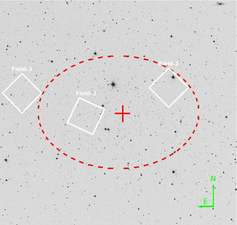
Figure 1: Location on the sky of the three HST fields (white boxes). Draco’s centre, half-light radius (shown as red cross and dashed red circle, respectively) and ellipticity are taken from Muñoz et al. (2018). The background $\sim 15\arcmin\times 15\arcmin$ image comes from the Sloan Digital Sky Survey.

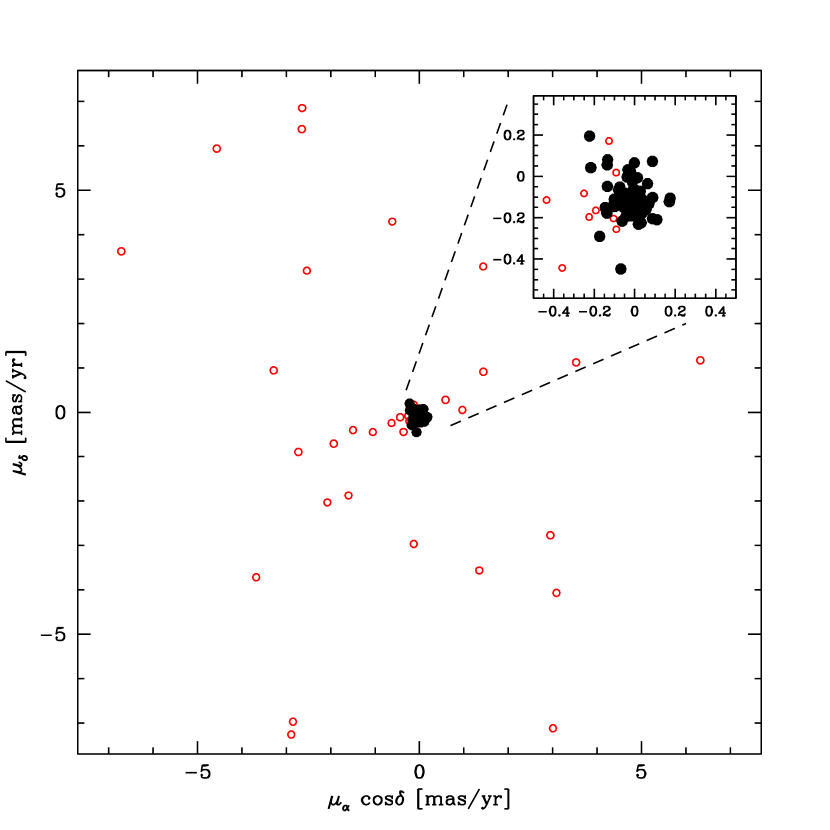
Figure 2: Vector point diagram for the sources in the direction of Draco with measured proper motions. Likely members are shown as black symbols, while likely foreground contaminants are marked with red empty symbols. The region zoomed around the bulk of likely Draco members is highlighted in the inset, where the few red symbols represent stars fainter than $G=20.8$ which are excluded from the analysis (see Sect.2).

2 Proper motions

Relative proper motions for Draco stars are measured from the combination of HST and Gaia positions. The first-epoch positional measurements come from observations acquired with the Wide Field Channel (WFC) of the Advanced Camera for Survey (ACS) on board HST. This camera consists of two $2048\times 4096$ pixel detectors, with a pixel scale of $\sim 0.05\arcsec\,$pixel^-1, and separated by a gap of about 50 pixels for a total field of view (FoV) $\sim 200\arcsec\times 200\arcsec$. The data set (GO-10229, PI: Piatek) consists of three pointings, located at $\sim 4\arcmin$, $\sim 5\arcmin$ and $\sim 11.7\arcmin$ distances from the dwarf nominal centre (Muñoz et al. 2018), as shown in Fig. 1. Each pointing was observed $19$ times, with each exposure having a duration of $430$ s. Exposures in Field-1 were taken in the F555W filter, while those in the other two fields were acquired in the F606W filter. The observations took place on the 30th and 31st of October, 2004.

The data reduction was performed using the img2xym$\_$WFC.09$\times$10 programme from Anderson & King (2006) on _FLC images, which were corrected for charge transfer efficiency (CTE) losses by the pre-reduction pipeline adopting the pixel-based correction described in Anderson & Bedin (2010); Ubeda & Anderson (2012). Each chip of each exposure was analysed independently using a pre-determined, filter-dependent model of the Point Spread Function (PSF), and for each chip we obtained a catalogue of all the unsaturated sources with positions, instrumental magnitudes, and PSF fitting-quality parameter. We used filter-dependent geometric distortions (Anderson 2007) to correct the stellar positions. The 19 catalogues of each field and chip were then rotated to be aligned with the equatorial reference frame and cross-matched using the stars in common for at least 15 of them. Once the coordinate transformations were determined, a catalogue containing average positions, magnitudes, and corresponding uncertainties (defined as the rms of the residuals around the mean value) for all of the sources detected in at least four individual exposures was created. In this way, at the end of the reduction we have six ACS/WFC catalogues, one per chip and field, ready to be matched with the Gaia second-epoch data.

Second-epoch positions are provided by the Gaia second data release (DR2, Gaia Collaboration et al. 2018a). This is a significant upgrade with respect to our previous work on the Sculptor dwarf spheroidal (M18) as DR2 is more complete than DR1 and allows us to have more faint stars in common between the two epochs because DR2 positions are more accurate and precise (the Gaia astrometric solution improves as more observations are collected with time, see Lindegren et al. 2018; Arenou et al. 2018). From the Gaia archive , we retrieved a catalogue with J2015.5 positions, related uncertainty and correlations, as well as magnitudes and astrometric excess noise for all the sources within a distance of $20\arcmin$ from the centre of Draco. In order to exclude sources with a clearly problematic solution from the analysis, we discarded all those with positional errors larger than $2$ mas (whereas the median positional uncertainty is $0.4$ mas). This dataset provides a total temporal baseline for proper-motion measurements of $10.593$ years.

As the final step in measuring the stellar proper motions, we transform HST first-epoch positions to the Gaia reference frame using a six-parameter linear transformation as described in M18. The difference between Gaia - and HST-transformed positions divided by the temporal baseline provides our proper-motion measurements, whereas the sum in quadrature between the two epochs’ positional errors divided by the same baseline provides the corresponding proper-motion uncertainties. We refined the coordinate transformations iteratively, each time using only likely members of Draco based on their location in the colour magnitude diagram (CMD) and the previous proper-motion determination. After three iterative steps, the procedure was converged (no stars were added or lost in the list used to compute the transformations in subsequent steps) and the final list of stellar proper motions was built, including $149$ sources. We bring these relative proper motions to an absolute reference frame using the Draco mean absolute motion of ($\mu_{\alpha}\cos(\delta),\mu_{\delta}$)$=(-0.019,-0.145)$ ${\rm mas/yr}$  as reported in Gaia Collaboration et al. (2018b).

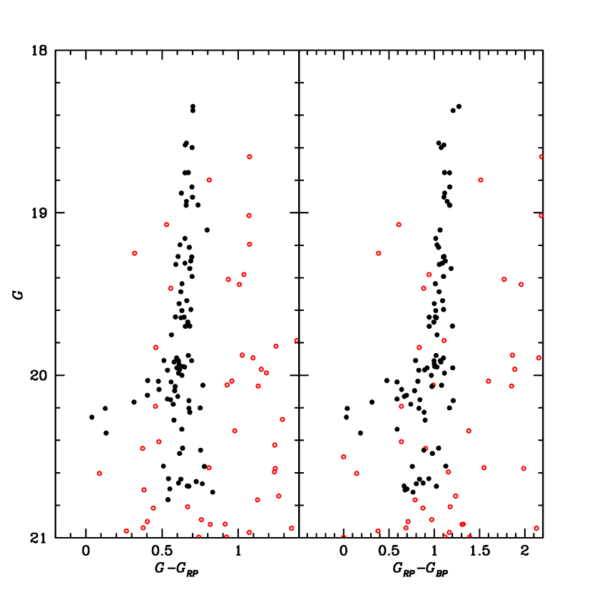
Figure 3: Gaia ($G$, $G$-$G_{\rm RP}$) and ($G$, $G_{\rm BP}$-$G_{\rm RP}$) colour magnitude diagrams. Likely members roughly selected from the VPD as described in the text are marked with black-filled symbols and correspond to those shown in Fig. 2.

The proper-motion measurements for all of the sources are shown in the Vector Point Diagram (VPD) in Fig. 2. The clump is centred around the Draco mean absolute motion, thus describing the likely members, and clearly separates them from the distribution of likely foreground stars, which have much larger proper motions. As a consistency check, Fig. 3 shows the Gaia ($G$, $G_{\rm RP}$) and ($G$, $G_{\rm BP}$-$G_{\rm RP}$) CMDs for the same sources. Black symbols indicate likely members, roughly selected as all the stars located within a 1 ${\rm mas/yr}$ distance from Draco’s absolute motion. They describe the well-defined sequences expected for the red giant and horizontal branches of Draco, whereas red symbols are mostly distributed in regions of the CMD populated by field stars. We note that this selection is not at all refined but has only been carried out as a first check that the proper-motion measurement procedure worked correctly. The final kinematic membership will be assessed after coupling the proper motions with radial velocity measurements.

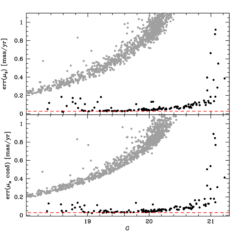
Figure 4: Intrinsic uncertainties as a function of Gaia $G$-band magnitude for the proper-motion component along $\alpha$ (lower panel) and $\delta$ (upper panel). Black-filled symbols are our HST+Gaia estimates, while grey-filled symbols are Gaia DR2 proper-motion uncertainties for sources in the direction of Draco. The red dashed line corresponds to a velocity of 10 km/s at the distance of Draco, roughly mimicking the system velocity dispersion.

Since our goal is to determine the velocity dispersion for the two proper-motion components in the plane of the sky, it is of primary importance to have all of the uncertainties, both statistical and systematic, under control.

Fig. 4 shows the distribution of the proper-motion statistical errors as a function of Gaia $G$-band magnitude. For comparison, grey symbols show Gaia DR2 proper-motion errors (on a baseline of $22$ months) for stars in the direction of the Draco dwarf spheroidal. The gain in precision obtained through our method is remarkable thanks to the larger baseline of $\sim 126$ month. At $G\simeq 19.5$, our measurements are one order of magnitude better than the Gaia DR2 proper motions alone and the improvement is even greater at fainter magnitudes.

To check for systematic effects, we look for possible trends between our relative proper-motion measurements and all the parameters entered into the analysis, such as Gaia colours, positions on the sky, HST magnitudes, location on the HST detector, etc. We always found consistency with no apparent trends within a 1-$\sigma$ uncertainty. In Fig. 5, we provide as an example the behaviour of the proper motions with respect to the Gaia $G_{\rm BP}$-$G_{\rm RP}$ colour. The only case where we find a significant systematic effect is when plotting the relative proper motion as a function of Gaia $G$ magnitude and this is shown in Fig. 6. This effect is only apparent for stars fainter than $G=20.8$ in the $\mu_{\alpha}\cos(\delta)$ versus G panel, with the proper motions being systematically negative. For this reason, we exclude all of the stars fainter than this (empty symbols in Fig. 6) from the analysis that follows. Note that these stars are also the ones with the largest statistical errors in Fig. 4 and that because of their faint magnitude, they will also lack a LOS velocity measurement, implying that in any case they would not be considered for the dynamical analysis presented later in this paper.

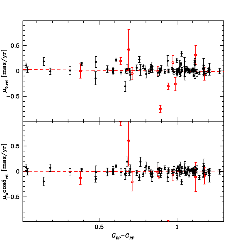
Figure 5: Trend of the two proper-motion components as a function of Gaia $G_{\rm BP}$-$G_{\rm RP}$ colour (same colour-coding as in Fig. 3). The best linear fits (red dashed lines) are not consistent with any trend among the uncertainties.

Figure 6: Trend for two components of the measured proper motions as a function of Gaia $G$-band magnitude (same colour-coding as in Fig. 3). The only systematic effect is visible for stars fainter than $G=20.8$, which are, therefore, excluded from the analysis. Red dashed lines show the best linear fit after their exclusion and show no trend among the uncertainties.

3 Line-of-sight velocities

Line-of-sight velocities (v_LOS) provide the third kinematic dimension needed for dynamical modelling. As a first step, we searched the literature for stars with available v_LOS measurements included in our proper-motion catalogue. By using the publicly available samples of Armandroff et al. (1995); Kleyna et al. (2002); Walker et al. (2015), consisting of more than two thousand measurements, we found a match for only 30 out of 149 stars, all based on the compilation from Walker et al. (2015). This is not surprising, due to the HST field of view being much smaller than the typical area sampled by spectroscopic surveys. Moreover, the stars for which we have proper motions are quite faint for spectroscopy and they can only be observed with 8-m class telescopes instrumentation to achieve a good signal-to-noise ratio (S/N$>10-15$) within a reasonable length of observing time.

It is for this reason that we targeted all of the stars in our proper-motion sample that are brighter than $G=20.8$ in a campaign with the DEIMOS spectrograph at the Keck II telescope. The strategy adopted to acquire the spectra is the same as that described in Massari et al. (2014a, b). We used the $1200$ line/mm grating, centred at $8000$ Å  (to retain the CaII triplet lines and avoid the inter-CCD gap) and coupled it with the GG$495$ and the GG$550$ order blocking filters. The slit width was chosen to be $0.75\arcsec$. In this way, we covered the range $6500-9500$Å  with a spectral resolution of R$\simeq 7000$ to sample prominent features like Ca triplet, H$\alpha$ and several strong metallic lines, which are all well-suited for v_LOS determination.

Since the field of view of each DEIMOS mask is approximately $16\arcmin\times 5\arcmin$, two out of three HST fields can be covered by a single pointing. Because of the high stellar density in the HST fields and the minimum slit length of 5 arcsec, we needed four masks to cover most of the desired targets, and to avoid issues of contamination from neighbouring targets. Some of the (faintest) targets had to be dropped because they could not fit any allowed mask configuration. Two mask configurations are shown in Fig. 7.

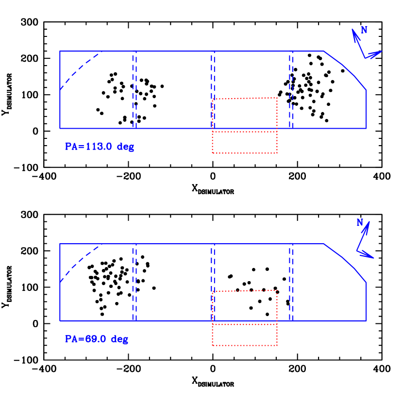
Figure 7: Here we show two of the DEIMOS masks. Blue lines outline the field of view of DEIMOS, with dashed lines separating individual chips. Blue arrows show the mask orientation on the sky. The red dotted square indicates DEIMOS guider. Black-filled symbols mark the available targets.

The observations were performed over two nights, on the 11th and 12th of August 2018 (Project code: U108, PI: Sales). In order to obtain a v_LOS precision comparable to or better than that of the tangential velocities, we observed each target with at least two $2100$ s long exposures (see Table 1).

Table 1: DEIMOS spectroscopic observations

Mask	Night	texp (s)	Seeing (″)
Mask-1A	August 11th	$2\times 2100$	0.8
Mask-2A	August 11th	$1\times 2100$	0.7
	August 12th	$1\times 2400$	0.7
	August 12th	$1\times 900$	0.7
Mask-1B	August 12th	$2\times 2400$	0.7
Mask-2B	August 12th	$2\times 2100$	0.7

One-dimensional spectra were extracted using the DEEP2 DEIMOS pipeline (Cooper et al. 2012; Newman et al. 2013). The software takes calibration (flat fields and arcs) and science images as input to produce output 1D spectra that are wavelength calibrated and combined. The frames are combined using an inverse-variance weighted algorithm to properly take account of different exposure times.

The LOS velocities of the observed stars were measured by cross-correlation against a synthetic template spectrum using the IRAF task fxcor. The template spectrum has been calculated with the SYNTHE code (Sbordone et al. 2004; Kurucz 2005), adopting atmospheric parameters typical for a metal-poor giant star in Draco, namely T${}_{\rm eff}\simeq 4500$ K, log g$=1.5$, [Fe/H]$=-2.0$. The synthetic template is convoluted with a Gaussian profile corresponding to the instrumental resolution of DEIMOS. Spectra that were either too contaminated by neighbours, or with too low of a S/N to be used to obtain a v_LOS measurement, were discarded from the analysis. All the v_LOS have been corrected for heliocentric motion. To check for possible wavelength calibration systematics, we also cross-correlated the observed spectra with synthetic spectra for the Earth’s atmosphere calculated with the code TAPAS (Bertaux et al. 2014) around the atmospheric absorption Fraunhofer A band ($7600$-$7700$ Å). We found an average offset of $2.8\pm 0.2$ km/s, which was applied to each spectrum.

Because of our desire to combine our set of v_LOS with that of Walker et al. (2015), a number of slits in each mask were used to observe targets in common to assess systematic offsets between the two samples. We thus calibrated the velocities obtained for each DEIMOS mask to the measurements by Walker et al. (2015). The offsets (ZP) are shown in Fig. 8, amounting to $ZP_{1A}=-9.6$ km/s ($\sigma_{ZP,1A}=3.5$ km/s); $ZP_{1B}=-8.5$ km/s ($\sigma_{ZP,1B}=4.1$ km/s); $ZP_{2A}=-9.3$ km/s ($\sigma_{ZP,2A}=3.6$ km/s); $ZP_{2B}=-8.9$ km/s ($\sigma_{ZP,2B}=1.6$ km/s). They are all consistent within 1$\sigma$, yet we decided to apply to the targets of each mask the appropriate zero-point (ZP) correction. We also checked that by applying the same zero-point to all of the target v_LOS, the results of the study do not change as the net effect is a change in the v_LOS dispersion by $\sim 0.05$ km/s.

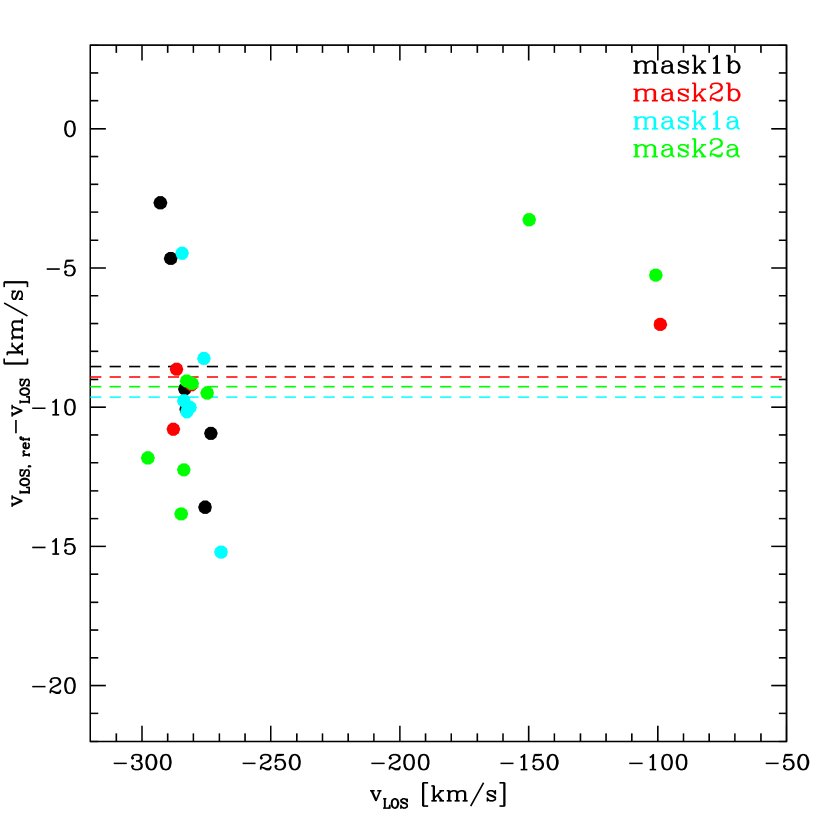
Figure 8: Offset between our measurements and those of Walker et al. (2015) for the targets in common. The colours mark different masks as indicated by the labels. Dashed lines are the adopted zero-points.

The intrinsic uncertainties in the measured v_LOS have been estimated with Monte Carlo simulations following the approach described in Simon & Geha (2007). We added Poisson noise to each pixel of one of the extracted 1D spectra with the highest S/N in order to reproduce different noise conditions. This procedure has been repeated to cover the entire range of S/N measured in the observed spectra, in steps of $\Delta$S/N$=10$. For each set of 300 ”noisy” spectra with a given S/N, v_LOS was measured with the procedure described above and the associated uncertainty $\epsilon_{LOS}$ was computed as the dispersion around the mean v_LOS value. In this way, we can derive a S/N-$\epsilon_{LOS}$ relation and use it to provide a v_LOS uncertainty to each observed spectrum, based on its S/N. The distribution of the intrinsic errors as a function of Gaia G magnitude is given in Fig. 9.

Figure 9: Intrinsic uncertainties on the LOS velocity as function of Gaia G-band magnitude.

As shown in Simon & Geha (2007) and Kirby et al. (2015), however, these intrinsic uncertainties do not take into account other possible sources of systematic effects. The first of these two papers quantified the systematic error to be 2.2 km/s, whereas the second paper reduced it to 1.5 km/s thanks to significant improvements in the standard reduction pipeline. Since we used the public version of the pipeline, we decided to add in quadrature the additional 2.2 km/s term quoted by Simon & Geha (2007) to the intrinsic uncertainties.

After the application of the offsets and the computation of the total uncertainty $\epsilon^{TOT}_{LOS}$, we computed the v_LOS for the stars in common between Walker et al. (2015) and our list using the weighted mean. Our final v_LOS catalogue thus includes $81$ stars (their distribution is the black histogram in Fig. 10), of which $51$ had never been targeted before, $18$ are in common with Walker et al. (2015), while the remaining $12$ come from Walker et al. (2015) only (red histogram in Fig. 10). The peak in the distribution defined by Draco-likely members emerges clearly from the rest and has a mean v_LOS of $-293.7\pm 1.2$ km/s, which is in good agreement with the Draco mean velocity of $-292.8\pm 0.5$ km/s found using the entire sample of Walker et al. (2015).

Figure 10: LOS velocity distribution for the entire sample of 81 stars. The red histogram shows the distribution of targets with LOS velocities coming from Walker et al. (2015) only. Grey dashed lines mark the boundaries of the adopted membership criterion.

The list of all the LOS velocities used here is given in Table 2, and is available in its entirety through the Centre de Données astronomiques de Strasbourg (CDS).

4 Velocity dispersions

With all the ingredients in hand, we selected the final sample of member stars with 3-D kinematics to be used to determine the velocity dispersions in the radial, tangential, and LOS direction. The criteria for a star to belong to such a sample are: $i$) $-326<$v${}_{LOS}<-260$ km/s (see the grey dashed lines in Fig. 10), meaning that a member is within $3.5$ times the dispersion around the mean receding velocity of Draco; $ii$) that the proper motion of a star differs from the mean proper motion of Draco by less than 1 ${\rm mas/yr}$. This corresponds to $\sim 360$ km/s at the distance of Draco and is about a factor of $50$ larger than the typical errors on the proper motions. Therefore, it is a very weak constraint that will not artificially affect the measurement of the velocity dispersion; $iii$) Gaia astrometric_excess_noise $<1$ to ensure that a source is a single star (and not an extended object or unresolved binary); $iv$) $G>19$ in order to avoid stars that are in the non-linear regime of the HST detector, where there may be systematic effects on their positional measurements.

We determined $45$ stars fulfilling these selection criteria and they will be used in the analysis below. Table 3 lists their positions, magnitudes, proper motions, v_LOS , and related errors for the first $10$ entries and is available in its entirety through CDS.

We then followed the prescriptions in M18 to determine the velocity dispersion on the plane of the sky. First, we transformed the proper motions from the measured equatorial reference to radial and tangential components according to the equatorial-polar coordinates relation in Binney & Tremaine (2008):

$$\left[\begin{array}[]{c}\mu_{R}\\ \mu_{T}\end{array}\right]=\begin{bmatrix}\cos(\phi)&\sin(\phi)\\ -\sin(\phi)&\cos(\phi)\end{bmatrix}\times\left[\begin{array}[]{c}\mu_{\alpha}\cos(\delta)\\ \mu_{\delta}\end{array}\right],$$

where $\phi=\arctan(y/x)$, and $x$ and $y$ are the (local Cartesian) gnomonic projected coordinates. Uncertainties are fully propagated, taking into account the correlation coefficient between the $\alpha$ and $\delta$ positions from Gaia. The projected velocities in the radial and tangential direction are, therefore, $v_{R,T}=4.74\mu_{R,T}d$, where we assumed $d=76$ kpc to be the distance to Draco (Bonanos et al. 2004).

We modelled the velocity dispersion for the sample of 45 stars using a multivariate Gaussian and including a covariance term. The parameters of the Gaussian are the velocity dispersions in the (projected) radial and tangential directions ($\sigma_{R},\sigma_{T}$), their correlation coefficient $\rho_{R,T}$ , and the mean velocities ($v_{0,R},v_{0,T}$). We used the Bayes theorem to derive the posterior distribution for these parameters. We assumed a weak Gaussian prior on the dispersions (centred on $10$ km/s and with $\sigma=3$ km/s) and on the correlation coefficient (with mean 0, and dispersion 0.8), and a flat prior for the mean velocities. The likelihood is a product of Gaussians, and the covariance matrix is the sum of the covariance matrices associated to the intrinsic kinematics of the population and to the measurement uncertainties (see equation 3 in the Methods Section of M18).

We used the Markov Chain Monte Carlo (MCMC) algorithm from Foreman-Mackey et al. (2013) to estimate the posterior for all the kinematic parameters and the results are shown in Fig. 11. For our sample, we find $\sigma_{R}=11.0^{+2.1}_{-1.5}$ km/s and $\sigma_{T}=9.9^{+2.3}_{-3.1}$ km/s, where the quoted errors correspond to the 16th and 84th percentiles. In our analysis, we have left the mean projected velocities $v_{0,R}$ and $v_{0,T}$ as free (nuisance) parameters, finding these values in good agreement with Draco’s estimated mean motion (Gaia Collaboration et al. 2018b).

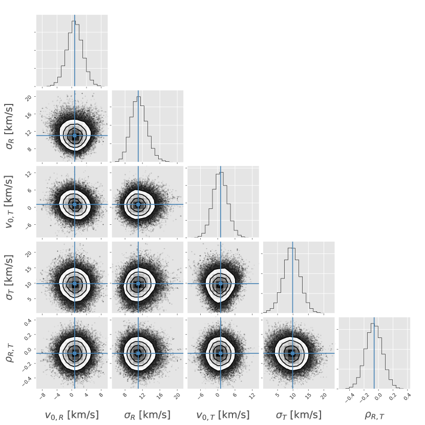
Figure 11: Corner plot for the modelled parameters. The maximum a posteriori value for each parameter is highlighted in blue.

To estimate the dispersion in the LOS velocity and its uncertainty, we applied the maximum-likelihood method described in Walker et al. (2006), finding $\sigma_{LOS}=9.0\pm 1.1$ km/s. This value is in good agreement with the LOS velocity dispersion profiles in Kleyna et al. (2002); Wilkinson et al. (2004); Walker et al. (2015) as per the location of our stars (the mean distance of our sample from Draco centre is R${}_{HST}\simeq 5.57\arcmin\simeq 120$ pc). We note that if we remove the subset of $8$ stars with v_LOS coming from Walker et al. (2015) from our final sample of $45$ stars, $\sigma_{LOS}$ changes by only $0.02$ km/s. This further demonstrates that the relative calibration between our measurements and theirs worked adequately.

5 Dynamical modelling

We now explore the constraints provided by our measurements on the internal dynamics of Draco. We focus on the velocity anisotropy $\beta$ and mass distribution, and, in particular, on the maximum circular velocity $V_{max}$. In what follows, we assume that our measurements of the velocity dispersions were obtained at the same location, namely at R_HST, which is the average projected distance from the centre of Draco.

5.1 A direct measurement of $\beta$

The velocity anisotropy is defined as $\beta(r)=1-(\sigma_{t}/\sigma_{r})^{2}$ (Binney 1980), where $\sigma_{t}(r)$ and $\sigma_{r}(r)$ are the intrinsic (3D) velocity dispersions in the tangential and radial directions, respectively. The anisotropy $\beta(r)$, the stellar 3D density profile of the stars $\nu_{\star}(r)$, and $\sigma_{r}(r)$ are related to the observed, projected velocity dispersions at projected distance $R$ as follows (Strigari et al., 2007a):

$$\sigma_{\rm los}^{2}(R)=\frac{2}{I_{\star}(R)}\int_{R}^{\infty}\left(1-\beta\frac{R^{2}}{r^{2}}\right)\frac{\nu_{\star}\sigma_{r}^{2}rdr}{\sqrt{r^{2}-R^{2}}}\,,$$ (1)

$$\sigma_{R}^{2}(R)=\frac{2}{I_{\star}(R)}\int_{R}^{\infty}\left(1-\beta+\beta\frac{R^{2}}{r^{2}}\right)\frac{\nu_{\star}\sigma_{r}^{2}rdr}{\sqrt{r^{2}-R^{2}}}\,,$$ (2)

$$\sigma_{T}^{2}(R)=\frac{2}{I_{\star}(R)}\int_{R}^{\infty}\left(1-\beta\right)\frac{\nu_{\star}\sigma_{r}^{2}rdr}{\sqrt{r^{2}-R^{2}}}.$$ (3)

From these equations, we can derive an estimate for the anisotropy at a radius $\hat{r}$ using the intermediate value theorem (see the full derivation in Massari et al. 2018):

$$\hat{\beta}=\beta(\hat{r})=1-\frac{\sigma^{2}_{T}}{\sigma^{2}_{\text{\rm LOS}}+\sigma^{2}_{R}-\sigma^{2}_{T}}\Bigg{\rvert}_{{\rm R}_{HST}}.$$ (4)

with $\hat{r}\in$ [R${}_{HST},r_{tid})$ and where $r_{tid}$ is the tidal radius of Draco (i.e. the stellar density is zero beyond this radial distance). This relation is also valid if we assume $\beta$ is constant (see M18).

Fig. 12 shows the posterior distribution for $\hat{\beta}$ obtained using our measurements and Eq. 4. This figure shows that radial anisotropies are favoured (although the uncertainties are large), with a median value of $\hat{\beta}=0.25^{+0.47}_{-1.38}$, and where the lower and upper limits correspond to the 16th and 84th percentiles of the distribution, respectively.

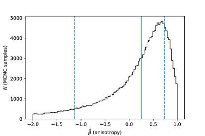
Figure 12: Posterior distribution for anisotropy $\hat{\beta}$ computed using Eq. 4. The median value is highlighted with the vertical solid line, whereas the 16th and 84th percentiles are highlighted with blue dashed lines. These have been computed using the whole range of possible anisotropies spanned by the distribution, even though this figure shows a shorter range for visualisation purposes.

5.2 Joint constraints on $V_{max}$ and $\beta$

We now use our measurements at R${}_{HST}\simeq 120$ pc to simultaneously constrain $\beta$ and $V_{max}$. To this end, we introduce the Jeans equation for a spherical system (Battaglia et al. 2013):

$$\sigma_{r}^{2}=\frac{GM(r)}{r}\frac{1}{\gamma-2\beta-\alpha},$$ (5)

where $\gamma=d\log\nu_{\star}/d\log r$, and $\alpha=d\log\sigma_{r}^{2}/d\log r$. For Draco, we may assume that $\alpha<<\gamma$ because its v_LOS dispersion profile is known to be relatively flat (e.g. Kleyna et al., 2002; Walker et al., 2009, 2015).

We compute $\sigma_{r}(r)$ from Eq. 5, for different mass models assuming different (constant) values of $\beta$. Replacing these in Eqs. 1, 2, and 3 allows us to derive confidence contours in the characteristic parameters of the models that are consistent with the measured values of the projected velocity dispersions.

We model the mass of the system as the sum of a dark and a stellar component. For the stellar component, we adopt a Plummer profile (Plummer 1911) with a projected half-light radius of R${}_{1/2}=196$ pc (Walker et al. 2007) and stellar mass of $3.2\times 10^{5}$ M_⊙ (Martin et al. 2008). For the dark halo component, we assume an NFW profile (Navarro et al. 1996b), for which

$$M(r)=4\pi\rho_{0}r_{s}^{3}[f(r/r_{s})]=M_{s}f(r/r_{s}),$$ (6)

where $\rho_{0}$ is a characteristic density, $r_{s}$ the scale radius, and $f(x)=\ln(1+x)-x/(1+x)$. The mass $M_{s}$ and the peak circular velocity $V_{max}$ are related via

$$M_{s}=\frac{R_{max}V_{max}^{2}}{{\rm G}f(2.163)},$$ (7)

where G is the gravitational constant, and where the peak circular velocity is at radius $R_{max}=2.163r_{s}$ for the NFW profile. On the other hand, the virial mass is $M(r_{vir})=M_{vir}=M_{s}f(c_{vir})$, where $c_{vir}=r_{vir}/r_{s}$.

Cosmological simulations have shown that there is a tight relation between the virial mass of a halo and its concentration $c_{vir}=r_{vir}/r_{s}$, such that the NFW profiles are effectively a one-parameter family (e.g. Bullock et al. 2001). For sub-haloes, that is, haloes surrounding satellite galaxies such as Draco, the concept of virial mass is ill-defined, however. This is why we prefer to work with the peak circular velocity $V_{max}$, which has been shown to vary little when a halo becomes a satellite (Kravtsov et al. 2004). For sub-haloes, there also is a relation between the mass-related parameter $V_{max}$ and a concentration parameter $c_{V}$ defined as (Diemand et al., 2007)

$$c_{V}=2\left(\frac{V_{max}}{H_{0}R_{max}}\right)^{2},$$ (8)

where $H_{0}$ is the Hubble constant, which we assume to be $H_{0}=70$ km/s/Mpc. Using high-resolution N-body cosmological simulations Moliné et al. (2017) found that

$$c_{V}=c_{0}[1+b\log(x_{sub})]\left[1+\sum_{i=1}^{3}\left[a_{i}\log\left(\frac{V_{max}}{\rm 10km/s}\right)\right]^{i}\right],$$ (9)

where $c_{0}=35000$, $a_{i}={-1.38,0.83,-0.49}$, $b=-2.5$ for a sub-halo located at the distance of Draco, that is, for d = $76$ kpc and the virial radius of the host halo to be $221.6$ kpc (McMillan 2017), for which $x_{sub}=0.34$.

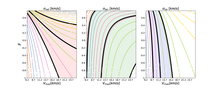
Figure 13: Velocity dispersion maps in the $V_{max}$-anisotropy space. Left, central and right panels show the velocity dispersions in the projected radial, tangential and in the LOS components, respectively. Black solid lines and coloured-shaded areas indicate the range defined by our mean measurements and their 16th and 84th percentiles, at R_HST. Coloured lines indicate contours of constant dispersion in steps of $0.5$ km/s.

We proceed to sample the space of parameters defined by ($V_{max}$, $\beta$). For each $V_{max}$ , we derive $R_{max}$ (and hence $r_{s}$) using Eqs. 8 and 9, and $M_{s}$ from Eq. 7. We then insert Eq. 6 (through Eq. 5) in Eqs. 1–3 to compute the predicted values of $\sigma_{LOS}$, $\sigma_{R}$ and $\sigma_{T}$ at R_HST for each pair of input parameters.

The three panels in Fig. 13 show the results of this procedure. Coloured lines indicate contours of constant dispersion in steps of $0.5$ km/s in the space of ($V_{max}$, $\beta$). In each panel, black solid lines mark the range defined by our mean measurements and the corresponding 16th and 84th percentiles (also highlighted by the coloured shaded areas). From Fig. 13 we note that at R_HST, $\sigma_{LOS}$ gives basically no constraint on $\beta$, whereas $\sigma_{R}$ is the most sensitive parameter in this respect. On the other hand, $\sigma_{LOS}$ provides the strongest information on the $V_{max}$ of the system, while $\sigma_{T}$ does so only for tangential anisotropy and becomes sensitive to $\beta$ for radial anisotropy.

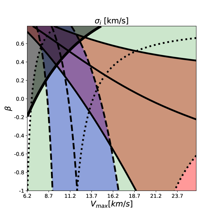
Figure 14: Three independent constraints coming from the measured velocity dispersions (from Fig. 13) over-plotted together. Their intersection (dark purple area) shows the range of allowed values for $V_{max}$ and constant anisotropy $\beta$.

To better highlight the constraints on $V_{max}$ and $\beta$ given by our measurements, we over-plot the three independent constraints in Fig. 14, using different line styles and colour-coding to demarcate each contribution. The three independent estimates all intersect in the darkest shaded region. The existence of a common solution demonstrates that our results are consistent with the NFW profile predicted by CDM models for the halo of Draco.

To check whether the entire range of parameters sampled by our solution is physically meaningful, we use the escape velocity expected for an NFW halo as a constraint (see Eq.16 from Shull, 2014) since $V_{esc}$ is related to $V_{max}$. Assuming stars in Draco follow a Gaussian velocity distribution, with a characteristic dispersion of $\sigma_{3D}=\sqrt{\sigma_{R}^{2}+\sigma_{T}^{2}+\sigma_{LOS}^{2}}$, we require that most of our stars in Draco be bound, that is, $3*\sigma_{3D}<V_{esc}$. At r=r_HST (where our measurements lie) this constraint results in a large portion of the ($V_{max},\beta$) plane being excluded. The allowed region is shown as a black-shaded area delimited by a thick solid line in Fig. 14. When taking this argument into account, we see that radial anisotropy seems to be preferred, although the allowed region extends down to $\beta\simeq-0.6$. This behaviour is fully consistent with the posterior distribution for $\hat{\beta}$ (Fig. 12) obtained directly from the data, but shows that different regions are preferred depending on the $V_{max}$ of the halo in which Draco is embedded. The range of preferred values for $V_{max}$ goes from $10.2$ km/s to $17.0$ km/s. This agrees within the errors with the previous estimate from Martinez (2015) who quote $V_{max}=18.2_{-1.6}^{+3.2}$ km/s, and it is consistent with the lower limits set by the analysis of Strigari et al. (2007b), who find $V_{max}>15$ km/s.

Fig. 15 shows the range of dark halo mass profiles for Draco that best describe our measurements. The grey shaded area has been derived using the range of $V_{max}$ values allowed by the joint constraints shown in Fig. 14 (together with the NFW profile given by Eq.6), while the green-shaded area corresponds to the range of profiles obtained when also taking into account the $1-\sigma$ scatter on the concentration relation (Eq. 9). Moliné et al. (2017) quote a scatter of $\sigma_{{\rm log}\leavevmode\nobreak\ c_{vir}}=0.11$. Since $c_{V}$ and $c_{vir}$ are related through

$$c_{V}=200\left(\frac{c_{vir}}{2.163}\right)^{3}\frac{f(R_{max}/r_{s})}{f(c_{vir})},$$ (10)

(Diemand et al., 2007), this implies that

$$\sigma_{{\rm log}c_{V}}\simeq\frac{\delta c_{V}}{c_{V}}=\left[3-\frac{c_{vir}^{2}}{(1+c_{vir})^{2}}\frac{1}{f(c_{vir})}\right]\frac{\delta c_{vir}}{c_{vir}},$$ (11)

which for the range of $V_{max}$ permitted by our measurements, results in $\sigma_{{\rm log}c_{V}}\simeq 2.54\sigma_{{\rm log}c_{vir}}$ or $\sigma_{{\rm log}\leavevmode\nobreak\ c_{V}}=0.28$.

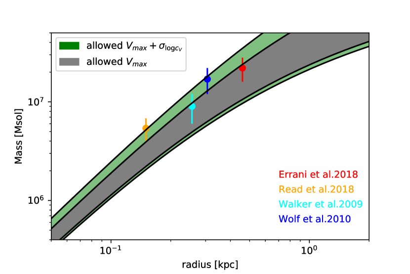
Figure 15: Comparison between our derived mass profile (grey shaded area) and previous mass estimates, colour-coded as indicated by the labels. Green-shaded area marks the range of mass allowed by our solution when also considering the scatter on the concentration relation.

We now compare the results of our mass modelling with published studies based on the use of line-of-sight velocities (see also Fig. 15). We first focus on three robust mass estimators which suffer little from the mass-anisotropy degeneracy. Walker et al. (2009) determine the mass enclosed within the projected half-light radius R_1/2, to be M${}_{1/2}=0.9\pm 0.3\times 10^{7}$ M_⊙. In comparison, we obtain $0.4\times 10^{7}<$ M${}_{1/2}<1.0\times 10^{7}$ M_⊙, for the $V_{max}$ range favoured by our measurements. Wolf et al. (2010) propose a mass estimator M${}_{-3}=3\sigma_{LOS}^{2}r_{-3}/G$, where $r_{-3}$ is the radius at which the logarithmic slope of the stellar density profile, ${\rm d}\log\nu_{\star}/{\rm d}\log r=-3$. For our measured $\sigma_{LOS}=9.0\pm 1.1$ km/s and for $r_{-3}=306$ pc, this yields M${}_{-3}=1.7\pm 0.5\times 10^{7}$ M_⊙, while the range of masses allowed by our models is $0.7\times 10^{7}<$ M${}_{-3}<1.3\times 10^{7}$ M_⊙. Note that the upper limit of our mass range increases to $1.8\times 10^{7}$ M_⊙ when considering the uncertainty on the mass-concentration relation. Finally, Errani et al. (2018) provide as an estimator the mass enclosed within 1.8 times R_1/2, defined as M${}_{1.8}=3.5\times 1.8$R${}_{1/2}\sigma_{LOS}^{2}/G$. According to our $\sigma_{LOS}$, this gives M${}_{1.8}=2.2\pm 0.7\times 10^{7}$ M_⊙, which is well within our range of solutions $1.0\times 10^{7}<$ M${}_{1.8}<2.3\times 10^{7}$ M_⊙.

Another interesting comparison is made with Read et al. (2018), who use the $\sigma_{LOS}$ profile find a spherically-averaged dark matter density at $r=150$ pc of $\rho_{DM}=2.4^{+0.5}_{-0.6}\times 10^{8}$ M_⊙ kpc^-3, which the authors argue favours the case for a cusp in Draco. In our case, given the allowed $V_{max}$ range and the scatter on the concentration relation, we find $0.8\times 10^{8}<\rho_{DM}<2.3\times 10^{8}$ M_⊙ kpc^-3, which is consistent with their estimate. It is worthwhile noticing that Read et al. (2018) infer a slightly tangential anisotropy and that, indeed, the similarity with our results is stronger when we consider the high mass side of our range (i.e. when our $\beta$ is more tangential).

Therefore, our mass models based on the use of proper motions and line-of-sight velocities of stars in Draco are in good agreement with published results from analytical estimators (Walker et al., 2009; Wolf et al., 2010) and with the more sophisticated modelling using the full line-of-sight velocity dispersion profile (e.g. Read et al., 2018). Still, our mass estimate tends to be closer to the lower limit of previously reported measurements (although well within the uncertainties). This could potentially indicate that Draco is more concentrated than has been predicted by the median $V_{max}$-concentration relation, which is also favoured by the analysis of Read et al. (2018). The latter work favoured a cold dark matter cusp for Draco mass profile. Our measurements and the consistent density estimate support the same conclusion.

6 Conclusions

In this paper, we present the first measurement of the velocity dispersion tensor of the Draco dwarf spheroidal galaxy. The proper motions on the plane of the sky were derived combining HST and Gaia data, following the procedure developed by M18 for the Sculptor dwarf spheroidal. We complemented the proper motions with $51$ new LOS velocity measurements from the DEIMOS spectrograph. After making a selection based on S/N and likely membership, we constructed a sample of $45$ stars having 3D velocities of exceptional quality (with typical errors on the individual 3D velocity $<10$ km/s). For this sample, located on average at 120 pc from the centre of Draco, we find dispersions of $\sigma_{R}=11.0^{+2.1}_{-1.5}$ km/s, $\sigma_{T}=9.9^{+2.3}_{-3.1}$ km/s, and $\sigma_{los}=9.0^{+1.1}_{-1.1}$ km/s. The uncertainties are almost a factor of two smaller than those in M18 for Sculptor.

These measurements allowed us to derive the posterior distribution of the orbital anisotropy $\beta$, at a radius $r\gtrsim$R_HST. This distribution is extended and peaks at $\hat{\beta}\sim 0.68$, with a median of $\hat{\beta}=0.25^{+0.47}_{-1.38}$, where the lower and upper limits indicate the 16th and 84th percentiles.

We also used these measurements to place simultaneous constraints on the $V_{max}$ of Draco and its orbital anisotropy (assuming the latter is constant). Using the Jeans equations (together with a requirement that the stars be bound) both for an NFW dark halo and a Plummer stellar profile, we find $V_{max}$ values in the range $10.2$ km/s to $17.0$ km/s, which is in good agreement with previous mass estimates based on LOS velocity measurements only. Although tangential anisotropy is allowed (up to $\beta\sim-0.6$), the range of allowed mass models is larger for radial anisotropy.

The fact that a family of solutions for Draco’s anisotropy and $V_{max}$ exist, given our 3D velocity dispersion measurements under the assumption of an NFW profile, demonstrates consistency with expectations drawn from cold dark matter models. More detailed dynamical modelling, together with more precise estimates on the 3D velocity dispersions, are required to establish firmer conclusions (see also Lazar, & Bullock 2019). Nonetheless, it is particularly encouraging that Gaia , as it continues its operations, is making proper-motion measurements ever more accurate. It should soon be possible to determine on more secure grounds whether the dark haloes of dwarf spheroidal galaxies follow the predictions of cosmological galaxy formation models.

Table 2: List of v_LOS measurements for Draco targets. Flag indicates whether the measurement is taken from (Walker et al., 2015, flag$=0$), if it is new (flag$=1$), or if it comes from the weighted mean between ours and Walker et al. (2015) measurements (flag$=2$). The entire list is available through the CDS.

$\alpha$	$\delta$	G	vLOS	$\epsilon^{TOT}_{v_{LOS}}$	flag
deg	deg		km/s	km/s
259.8451248562	57.9478908265	19.380	-300.7	2.5	1
259.8192040232	57.9691005474	18.930	-289.8	2.3	2
259.8417154779	57.9840860321	19.197	-298.4	2.6	2
259.8884861598	57.9438841701	19.318	-286.1	2.5	2
259.8647236300	57.9442576339	20.178	-311.0	3.8	1
259.8225679085	57.9641182530	20.191	-219.3	2.9	1
259.9216037743	57.9618490671	18.346	-302.5	2.6	1
259.8598480665	57.9932178145	18.599	-299.4	2.8	1
259.9041829235	57.9631190310	18.954	-286.6	2.5	1
259.9215205028	57.9811054827	19.194	+0.4	2.8	1

Table 3: List of positions, Gaia G-band magnitude, $\mu_{\alpha}\cos(\delta)$, $\mu_{\delta}$, v_LOS and related uncertainties for sample of 45 stars with 3D motions used in the dynamical analysis. The entire list is available through the CDS.

$\alpha$	$\delta$	G	$\mu_{\alpha}\cos(\delta)$	$\epsilon_{\mu_{\alpha}\cos(\delta)}$	$\mu_{\delta}$	$\epsilon_{\mu_{\delta}}$	vLOS	$\epsilon^{TOT}_{v_{LOS}}$
deg	deg		${\rm mas/yr}$	${\rm mas/yr}$	${\rm mas/yr}$	${\rm mas/yr}$	km/s	km/s
259.8417154779	57.9840860321	19.197	-0.027	0.034	-0.154	0.028	-298.4	2.6
259.8568904104	57.9515551582	19.269	0.014	0.032	-0.176	0.032	-308.5	1.4
259.8884861598	57.9438841701	19.318	-0.054	0.044	-0.117	0.038	-286.1	2.5
259.8647236300	57.9442576339	20.178	-0.048	0.052	-0.103	0.056	-311.0	3.8
259.8722406668	57.9796046445	19.297	0.014	0.052	-0.178	0.035	-309.1	2.9
259.8666938634	57.9941772891	19.392	-0.012	0.032	-0.143	0.030	-290.4	3.0
259.9192783256	57.9774115703	20.069	-0.043	0.050	-0.170	0.055	-298.5	2.9
259.8789532265	57.9830671561	20.150	-0.063	0.056	-0.135	0.058	-315.5	2.9
259.9211108657	57.9681922763	20.201	-0.056	0.058	-0.117	0.053	-302.0	3.0
259.8645763982	57.9846580785	20.204	-0.025	0.065	-0.139	0.055	-286.6	4.9