The giants arcs as modeled by the superbubbles

Abstract

The giant arcs in the clusters of galaxies are modeled in the framework of the superbubbles. The density of the intracluster medium is assumed to follow a hyperbolic behavior. The analytical law of motion is function of the elapsed time and the polar angle. As a consequence the flux of kinetic energy in the expanding thin layer decreases with increasing polar angle making the giant arc invisible to the astronomical observations. In order to calibrate the arcsec-parsec conversion three cosmologies are analyzed.

Keywords: galaxy groups, clusters, and superclusters; large scale structure of the Universe Cosmology

1 Introduction

The giant arcs in the cluster of galaxies start to be observed as narrow-like shape by [1, 2, 3] and the first theoretical explanation was the gravitational lensing, see [4, 5, 6, 7]. The determination of the statistical parameters of the giant arcs has been analyzed in order to derive the cosmological parameters, see [8], in connection with the $\Lambda$CDM cosmology, see [9], in the framework of the triaxiality and substructure of CDM halo, see [10], in connection with the Wilkinson Microwave Anisotropy Probe (WMAP) data, see [11], including the effects of baryon cooling in dark matter N-body simulations, see [12] and in order to derive the photometric properties of 105 giant arcs that in the Second Red-Sequence Cluster Survey (RCS-2), see [13]. The gravitational lensing is the most common theoretical explanation, we select some approaches among others: [14] evaluated the mass distribution inside distant clusters, [15] studied the statistics of giant arcs in flat cosmologies with and without a cosmological constant, [16] analyzed how the gravitational lensing influences the surface brightness of giant luminous arcs and [17] used the warm dark matter (WDM) cosmologies to explain the lensing in galaxy clusters. Another theoretical line of research explains the giant arcs as shells originated by the galaxies in the cluster: [18, 19] analyzed the the limb-brightened shell model, the gravitational lens model and the echo model, [20] suggested that the Gamma-ray burst (GRB) explosions are the sources of the shells with sizes of many kpc, and [21] suggested a connection between the Einstein ring associated to SDP.81 and the evolution of a superbubble (SB) in the intracluster medium.

This paper analyzes in Section 2 three cosmologies in order to calibrate the transversal distance which allows to convert the arcsec in pc. Section 3 is devoted to the evolution of a SB in the intracluster medium. Section 4 reports the observations of the giant arcs and the first phase of a SB. Section 5 reports the various steps which allow to reproduce the shape of the giant arc A2267 and the multiple arcs visible in the cluster of galaxies. Section 6 is dedicated to theory of the image: analytical formulae explain the hole in the central part of the SBs and numerical results reproduce the details of a giant arc.

2 Adopted cosmologies

In the following we review three cosmological theories.

2.1 $\Lambda$CDM cosmology

The basic parameters of $\Lambda$CDM cosmology are: the Hubble constant, $H_{0}$, expressed in $\mathrm{km\,s^{-1}\,Mpc^{-1}}$, the velocity of light, $c$, expressed in $\mathrm{km\,s^{-1}}$, and the three numbers $\Omega_{\rm M}$, $\Omega_{K}$, and $\Omega_{\Lambda}$, see [22] for more details. In the case of the Union 2.1 compilation, see [23], the parameters are $H_{0}=69.81\mathrm{km\,s^{-1}\,Mpc^{-1}}$, $\Omega_{\rm M}=0.239$ and $\Omega_{\Lambda}=0.651$. To have the luminosity distance, $D_{L}(z;H_{0},c,\Omega_{\rm M},\Omega_{\Lambda})$, as a function of the redshift only, we apply the minimax rational approximation, which is characterized by two parameters, $p$ and $q$. The luminosity distance, $D_{L,3,2}$, when $p=3$ and $q=2$

$$D_{L,3,2}=\frac{-7.761-1788.53\,z-3203.06\,{z}^{2}-65.8463\,{z}^{3}}{-0.438025-0.334872\,z+0.0203996\,{z}^{2}}\,Mpc$$ (1)

$$\quad for\quad 0.001<z<4\quad.$$

The transversal distance in $\Lambda$CDM cosmology, $D_{T,3,2}$, which corresponds to the angle $\delta$ expressed in arcsec is

$$D_{T,3,2}=\frac{4.84813\,{\it\delta}\,\left(2.328+502.067\,z+113.03\,{z}^{2}\right)}{0.124085+0.149501\,z+0.0932928\,{z}^{2}}\,pc\quad.$$ (2)

2.2 Flat Cosmology

The two parameters of the flat cosmology are $H_{0}$, the Hubble constant expressed in $\mathrm{km\,s^{-1}\,Mpc^{-1}}$, and $\Omega_{\rm M}$ which is

$$\Omega_{\rm M}=\frac{8\pi\,G\,\rho_{0}}{3\,H_{0}^{2}}\quad,$$ (3)

where $G$ is the Newtonian gravitational constant and $\rho_{0}$ is the mass density at the present time. In the case of $m$=2 and $n$=2 the minimax rational expression for the luminosity distance, $d_{L,m,2,2}$, when $H_{0}=70\,\mathrm{km\,s^{-1}\,Mpc^{-1}}$ and $\Omega_{\rm M}=0.277$, is

$$d_{L,m,2,2}=\frac{0.0889+748.555\,z+5.58311\,{z}^{2}}{0.175804+0.206041\,z+0.068685\,{z}^{2}}\,Mpc\quad.$$ (4)

The transversal distance in flat cosmology, $D_{Tf,3,2}$, which corresponds to the angle $\delta$ expressed in arcsec is

$$D_{Tf,3,2}=\frac{4.84813\,{\it\delta}\,\left(0.0889+748.555\,z+5.58311\,{z}^{2}\right)}{0.175804+0.206041\,z+0.0686854\,{z}^{2}}\,pc$$ (5)

2.3 Modified tired light

In an Euclidean static framework the modified tired light (MTL) has been introduced in Section 2.2 in [24]. The distance in MTL is

$$d=\frac{c}{H_{0}}\ln(1+z)\quad.$$ (6)

The distance modulus in the modified tired light (MTL) is

$$m-M=\frac{5}{2}\,{\frac{\beta\,\ln\left(z+1\right)}{\ln\left(10\right)}}+5\,{\frac{1}{\ln\left(10\right)}\ln\left({\frac{\ln\left(z+1\right)c}{H_{{0}}}}\right)}+25\quad.$$ (7)

Here $\beta$ is a parameter comprised between 1 and 3 which allows to match theory with observations. The number of free parameters in MTL is two: $H_{0}$ and $\beta$. The fit of the distance modulus with the data of Union 2.1 compilation gives $\beta$=2.37, $H_{0}=69.32\pm 0.34$, see [22], which means the following distance

$$d=4324.761\,\ln\left(1+z\right)\left(1+z\right)^{1.185}\,Mpc\quad.$$ (8)

The transversal distance in MTL, $d_{T}$, which corresponds to the angle $\delta$ expressed in arcsec is

$$d_{T}=20967\,{\it\delta}\,\ln\left(1+z\right)\left(1+z\right)^{1.185}\,pc$$ (9)

We report the angular distance for a fixed $delta$ as function of redshift for the three cosmologies, see Figure 1. The angular distance in flat and $\Lambda$CDM cosmology does not increase with z, see [25], in contrast with the modified tired light .

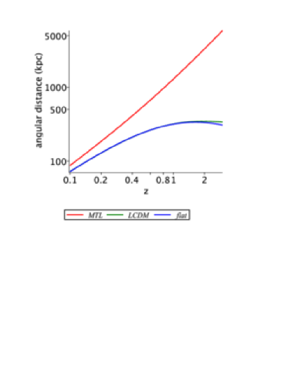
Figure 1: Angular distances in kpc for the three cosmologies here considered when $\delta=38.913456$

3 The motion of a SB

We now summarize the adopted profile of density and the equation of motion for a SB.

3.1 The profile

The density is assumed to have the following hyperbolic dependence on $Z$ which is the third Cartesian coordinate,

$$\rho(Z;Z_{0},\rho_{0})=\left\{\begin{array}[]{ll}\rho_{0}&\mbox{if z $\leq Z_{0}$ }\\ \rho_{0}\frac{Z_{0}}{z}&\mbox{if z $>Z_{0}$ }\\ \end{array}\right.$$ (10)

where the parameter $Z_{0}$ fixes the scale and $\rho_{0}$ is the density at $Z=Z_{0}$. In spherical coordinates the dependence on the polar angle is

$$\rho(r;\theta,Z_{0},\rho_{0})=\left\{\begin{array}[]{ll}\rho_{0}&\mbox{ if $\cos(\theta)\leq Z_{0}$}\\ \rho_{0}\frac{Z_{0}}{r\cos(\theta)}&\mbox{if $r\cos(\theta)>Z_{0}$}\\ \end{array}\right.$$ (11)

Given a solid angle $\Delta\Omega$ the mass $M_{0}$ swept in the interval $[0,r_{0}]$ is

$$M_{0}=\frac{1}{3}\,\rho_{{0}}\,{r_{{0}}}^{3}\Delta\Omega\quad.$$ (12)

The total mass swept, $M(r;r_{0},Z_{0},\alpha,\theta,\rho_{0})$, in the interval $[0,r]$ is

$$M(r;r_{0},Z_{0},\alpha,\theta,\rho_{0})=\bigl{(}\frac{1}{3}\,\rho_{{0}}{r_{{0}}}^{3}+\frac{1}{2}\,{\frac{\rho_{{0}}Z_{{0}}\left({r}^{2}-{r_{{0}}}^{2}\right)}{\cos\left(\theta\right)}}\bigr{)}\Delta\Omega\quad.$$ (13)

and its approximate value at high values of $r$ is

$$M(r;Z_{0},\alpha,\theta,\rho_{0})\approx\frac{1}{2}\,{\frac{{r}^{2}\rho_{{0}}Z_{{0}}}{\cos\left(\theta\right)}}\Delta\Omega\quad.$$ (14)

The density $\rho_{0}$ can be obtained by introducing the number density, $n_{0}$, expressed in particles $\mathrm{cm}^{-3}$, the mass of hydrogen, $m_{H}$, and a multiplicative factor $f$, which is chosen to be 1.4, see [26],

$$\rho_{0}=fm_{H}n_{0}\quad.$$ (15)

The astrophysical version of the total approximate swept mass as given by equation (14), expressed in solar mass units, $M_{\odot}$, is

$$M(r_{pc};Z_{0,pc},n_{0},\theta)\approx\frac{0.0172\,n_{{0}}{z}_{{{0,pc}}}{r_{{{pc}}}}^{2}}{cos(\theta)}\,M_{\odot}\,\Delta\Omega\quad,$$ (16)

where $Z_{0,pc}$, and $r_{0,pc}$ are $Z_{0}$, and $r$ expressed in pc.

3.2 The equation of motion

The conservation of the classical momentum in spherical coordinates along the solid angle $\Delta\Omega$ in the framework of the thin layer approximation states that

$$M_{0}(r_{0})\,v_{0}=M(r)\,v\quad,$$ (17)

where $M_{0}(r_{0})$ and $M(r)$ are the swept masses at $r_{0}$ and $r$, and $v_{0}$ and $v$ are the velocities of the thin layer at $r_{0}$ and $r$. This conservation law can be expressed as a differential equation of the first order by inserting $v=\frac{dr}{dt}$:

$$M(r)\,\frac{dr}{dt}-M_{0}\,v_{0}=0\quad.$$ (18)

The velocity as a function of the radius $r$ is

$$v(r;r_{0},Z_{0},v_{0},\theta)=2\,{\frac{{r_{{0}}}^{3}v_{{0}}\cos\left(\theta\right)}{2\,{r_{{0}}}^{3}\cos\left(\theta\right)-3\,{r_{{0}}}^{2}Z_{{0}}+3\,{r}^{2}Z_{{0}}}}\quad.$$ (19)

The differential equation which models the momentum conservation in the case of a hyperbolic profile is

$$\left(\frac{1}{3}\,{r_{{0}}}^{3}+\frac{1}{2}\,{\frac{Z_{{0}}\left(-{r_{{0}}}^{2}+\left(r\left(t\right)\right)^{2}\right)}{\cos\left(\theta\right)}}\right){\frac{\rm d}{{\rm d}t}}r\left(t\right)-\frac{1}{3}\,{r_{{0}}}^{3}v_{{0}}=0\quad,$$ (20)

where the initial conditions are $r=r_{0}$ and $v=v_{0}$ when $t=t_{0}$.

The variables can be separated and the radius as a function of the time is

$$r(t;t_{0},r_{0},Z_{0},v_{0},\theta)=\frac{HN}{HD}\quad,$$

where

$$HN=-\sqrt[3]{3}\Bigg{(}2\,\cos(\theta)\sqrt[3]{3}r_{{0}}-3\,\sqrt[3]{3}Z_{{0}}-\bigg{(}-9\,{Z_{{0}}}^{3/2}+((9\,t-9\,t_{{0}})v_{{0}}$$

$$+9\,r_{{0}})\cos(\theta)\sqrt{Z_{{0}}}+\sqrt{3}\sqrt{27}\sqrt{{\it AHN}}\bigg{)}^{2/3}\Bigg{)}r_{{0}}\quad,$$ (21)

with

$$AHN=\Bigg{(}{\frac{8\,(\cos(\theta))^{2}{r_{{0}}}^{3}}{27}}$$

$$+Z_{{0}}\bigg{(}(t-t_{{0}})^{2}{v_{{0}}}^{2}+2\,r_{{0}}(t-t_{{0}})v_{{0}}-\frac{1}{3}\,{r_{{0}}}^{2}\bigg{)}\cos(\theta)$$

$$-2\,v_{{0}}{Z_{{0}}}^{2}(t-t_{{0}})\Bigg{)}\cos(\theta)$$ (22)

and

$$HD=3\,\sqrt{Z_{{0}}}\times$$

$$\sqrt[3]{-9\,{Z_{{0}}}^{3/2}+\left(\left(9\,t-9\,t_{{0}}\right)v_{{0}}+9\,r_{{0}}\right)\cos\left(\theta\right)\sqrt{Z_{{0}}}+9\,\sqrt{{\it BHD}}}\quad,$$ (23)

with

$$BHD=\Bigg{(}{\frac{8\,(\cos(\theta))^{2}{r_{{0}}}^{3}}{27}}+$$

$$Z_{{0}}\bigg{(}(t-t_{{0}})^{2}{v_{{0}}}^{2}+2\,r_{{0}}(t-t_{{0}})v_{{0}}-\frac{1}{3}\,{r_{{0}}}^{2}\bigg{)}\cos(\theta)$$

$$-2\,v_{{0}}{Z_{{0}}}^{2}(t-t_{{0}})\Bigg{)}\cos(\theta)\quad.$$ (24)

As a consequence the velocity as function of the time is

$$v(t;t_{0},r_{0},Z_{0},v_{0},\theta)=\frac{dr(t;t_{0},r_{0},Z_{0},v_{0},\theta)}{dt}\quad.$$

More details as well the exploration of other profiles of density can be found in [27]. We now continue evaluating the flux of kinetic energy, $F_{ek}$, in the thin emitting layer which is supposed to have density $\rho_{l}$

$$F_{ek}(t;t_{0},r_{0},Z_{0},v_{0},\theta)=\frac{1}{2}\rho_{l}4\pi r(t)^{2}v(t)^{3}\quad.$$ (25)

The volume of the thin emitting layer, $V_{l}$, is approximated by

$$V_{l}=4\,{\it\Delta}\,\pi\,{r}^{2}\quad,$$ (26)

where $\Delta$ is thickness of the layer; as an example [26] quotes $\Delta=\frac{r}{12}$. The two approximations for mass, equation (14), and volume, equation (26), allows to derive an approximate value for the density in the thin layer

$$\rho_{l}=\frac{1}{8}\,{\frac{\rho_{{0}}Z_{{0}}f}{\cos\left(\theta\right)r\pi}}\quad.$$ (27)

Inserted in equation (25) the radius, velocity and density as given by equations (3.2), (3.2) and (27), we obtain

$$F_{ek}(t;t_{0},r_{0},Z_{0},v_{0},\theta)=\frac{FN}{FD}\quad,$$ (28)

where

$$FN=\quad,-\sqrt{27}\left(-3\,\sqrt{3}{Z_{{0}}}^{3/2}+\sqrt{27}\sqrt{F_{{1}}\cos\left(\theta\right)}+3\,F_{{5}}\right)^{3}f\times$$

$$\left(2\,\sqrt[3]{3}F_{{3}}+\left(-9\,{Z_{{0}}}^{3/2}+F_{{2}}+\sqrt{27}\sqrt{F_{{1}}\cos\left(\theta\right)}\sqrt{3}\right)^{2/3}\right)^{3}{r_{{0}}}^{4}\times$$

$$\cos\left(\theta\right){{\it v0}}^{3}\sqrt{Z_{{0}}}\bigg{(}2\,\sqrt[3]{3}F_{{3}}-\big{(}-9\,{Z_{{0}}}^{3/2}+F_{{2}}+$$

$$\sqrt{27}\sqrt{F_{{1}}\cos(\theta)}\sqrt{3}\big{)}^{2/3}\bigg{)}\sqrt[3]{3}\rho_{{0}}$$ (29)

and

$$FD=108\,\sqrt{F_{{1}}\cos\left(\theta\right)}\times$$

$$\left(-9\,{Z_{{0}}}^{3/2}+F_{{2}}+\sqrt{27}\sqrt{F_{{1}}\cos\left(\theta\right)}\sqrt{3}\right)^{13/3}F_{{4}}$$ (30)

being

$$F_{1}={\frac{8\left(\cos\left(\theta\right)\right)^{2}{r_{{0}}}^{3}}{27}}+\left(\left(t-t_{{0}}\right)^{2}{{\it v0}}^{2}+2r_{{0}}\left(t-t_{{0}}\right){\it v0}-\frac{1}{3}{r_{{0}}}^{2}\right)\times$$

$$Z_{{0}}\cos\left(\theta\right)-2{\it v0}{Z_{{0}}}^{2}\left(t-t_{{0}}\right)\quad,$$ (31)

$$F_{2}=\left(\left(9t-9t_{{0}}\right){\it v0}+9r_{{0}}\right)\cos\left(\theta\right)\sqrt{Z_{{0}}}\quad,$$ (32)

$$F_{3}=\cos\left(\theta\right)r_{{0}}-3/2Z_{{0}}$$ (33)

$$F_{4}=8\,(\cos(\theta))^{2}{r_{{0}}}^{3}+27\,\Bigr{(}(t-t_{{0}})^{2}{{\it v0}}^{2}+2\,r_{{0}}(t-t_{{0}}){\it v0}-$$

$$\frac{1}{3}\,{r_{{0}}}^{2}\Bigl{)}Z_{{0}}\cos(\theta)-54\,{\it v0}\,{Z_{{0}}}^{2}(t-t_{{0}})\quad,$$ (34)

$$F_{5}=\left({\it v0}\,\left(t-t_{{0}}\right)+r_{{0}}\right)\cos\left(\theta\right)\sqrt{3}\sqrt{Z_{{0}}}\quad.$$ (35)

We now assumes that the amount of luminosity, $L_{theo}$, reversed in the shocked emission is proportional to the flux of kinetic energy as given by equation (28)

$$L_{theo}(t;t_{0},r_{0},Z_{0},v_{0},\theta)\propto F_{ek}(t;t_{0},r_{0},Z_{0},v_{0},\theta)\quad.$$ (36)

The theoretical luminosity is not equal along all the SB but is function of the polar angle $\theta$. In this framework is useful to introduce the ratio, $\kappa$, between theoretical luminosity at $\theta$ and and that one at $\theta=0$,

$$\kappa=\frac{L_{theo}(t;t_{0},r_{0},Z_{0},v_{0},\theta)}{L_{theo}(t;t_{0},r_{0},Z_{0},v_{0},\theta=0)}\quad.$$ (37)

The above model for the theoretical luminosity is independent from the image theory, see Section 6, and does not explains the hole of luminosity visible in the shells.

4 Astrophysical Environment

We now analyze the catalogue for the giant arcs, the two giant arcs SDP.81 and A2267 and the initial astrophysical conditions for the SBs.

4.1 The catalogue

Some parameters of the giant arcs as detected as images by cluster lensing and the supernova survey with Hubble (CLASH) which is available as a catalogue at http://vizier.u-strasbg.fr/viz-bin/VizieR, see [28]. We are interested in the arc length which is given in arcsec, the arc length to width ratio, the photometric redshift, and in the radial distance from the arc center to the cluster center in arcsec. Table 1 reports the statistical parameters of the radial distance from the arc center to the cluster center in kpc and Figure 2, Figure 3, and Figure 4 the histogram of the frequencies in the framework of flat,$\Lambda$CDM and MTL cosmology respectively.

Table 1: Statistical parameters of the radial distance from the arc center to the cluster center in kpc

Cosmology	minimum (kpc)	average (kpc)	maximum (Mpc)
Flat	89	270	313
$\Lambda$CDM	89	288	323
MTL	7	3810	1540

Figure 2: Histogram of the radial distance from the arc center to the cluster center in Mpc in flat cosmology with conversion formula (5).

Figure 3: Histogram of the radial distance from the arc center to the cluster center in Mpc in $\Lambda$CDM cosmology with conversion formula (2).

Figure 4: Histogram of the radial distance from the arc center to the cluster center in Mpc in MTL cosmology with conversion formula (9).

4.2 Single giant arcs

The ring associated with the galaxy SDP.81, see [29], is characterized by a foreground galaxy at $z=0.2999$ and a background galaxy at $z=0.3042$. This ring has been studied with the Atacama Large Millimeter/sub-millimeter Array (ALMA) by [30, 31, 32, 33, 34, 35] and has the observed parameters as in Table 2.

Table 2: Observed parameters of the giants arcs.

Name	redshift	radius arcsec
SDP.81	3.04	1.54
A2667	1.033	42

Another giant arc is that in A2667 which is made by three pieces: A, B and C , see Figure 1 in [36]. The radius can be found from the equation of the circle given the three points A, B and C, see Table 3. The three pieces can be digitalized for a further comparison with a simulation, see empty red stars in Figure 8.

Table 3: Radius of the giant arcs in kpc.

Cosmology	SDP.81	A2667
Flat	12.09	345.39
$\Lambda$CDM	13.33	347.42
MTL	235.82	1456.32

4.3 The initial conditions

We review the starting equations for the evolution of the SB [37, 38, 39] which can be derived from the momentum conservation applied to a pyramidal section. The parameters of the thermal model are $N^{*}$, the number of SN explosions in $5.0\cdot 10^{7}$ yr, $Z_{\mathrm{OB}}$, the distance of the OB associations from the galactic plane, $E_{51}$, the energy in $10^{51}$ erg usually chosen equal to one, $v_{0}$, the initial velocity which is fixed by the bursting phase, $t_{0}$, the initial time in $yr$ which is equal to the bursting time, and $t$ the proper time of the SB. With the above definitions the radius of the SB is

$$R=111.56\,(\frac{E_{51}t_{7}^{3}N^{*}}{n_{0}})^{\frac{1}{5}}\,\mathrm{pc},$$ (38)

and its velocity

$$V=6.567\,{\frac{1}{{{\it t_{7}}}^{2/5}}\sqrt[5]{{\frac{E_{{51}}{\it N^{*}}}{n_{{0}}}}}}\,\mathrm{\frac{km}{s}}\quad.$$ (39)

In the following, we will assume that the bursting phase ends at $t=t_{7,0}$ (the bursting time is expressed in units of $10^{7}$ yr) when $N_{SN}$ SN are exploded

$$N_{SN}=N^{*}\frac{t_{7,0}\cdot 10^{7}}{5\cdot 10^{7}}\quad.$$ (40)

The two following inverted formula allows to derive the parameters of the initial conditions for the SB with ours $r_{0}$ expressed in pc and $v_{0}$ expressed in $km\,s^{-1}$ are

$$t_{7,0}=0.05878095238\,{\frac{r_{{0}}}{v_{{0}}}}\quad,$$ (41)

and

$$N^{*}=2.8289\,10^{-7}\,{\frac{{r_{{0}}}^{2}n_{{0}}{v_{{0}}}^{3}}{E_{{51}}}}\quad.$$ (42)

5 Astrophysical Simulation

We simulate a single giant arc, A2267, and then we simulate the statistics of many giant arcs.

5.1 Simulation of A2667

The final stage of the SB connected with A2267 is simulated with the parameters reported in Table 4 ; in particular Figure 5 displays the 3D shape and Figure 6 reports the 2D section.

Table 4: Theoretical parameters of the SB connected with A2267.

theory	parameter	value
initial thermal model	$E_{51}$	1
initial thermal model	$n_{0}$	1
initial thermal model	$t_{7,0}$	0.0078
initial thermal model	$N^{*}$	$1.22\,10^{14}$
initial thermal model	$N_{SN}$	$1.91\,10^{11}$
SB	$r_{0}$	4000 pc
SB	$Z_{0}$	74.07 pc
SB	$v_{0}$	30000 km/s
SB	t	$8\,10^{8}$ yr

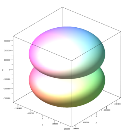
Figure 5: 3D surface of the SB connected with A2267, parameters as in Table 4 and axes in pc.

Figure 6: 2D section in the $z=0$ plane of the SB connected with A2267, parameters as in Table 4 and axes in kpc.

Figure 7 reports the 2D section of the SB as well the three pieces of the giant arc connected with A2267.

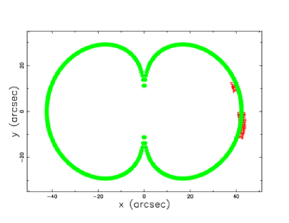
Figure 7: 2D section in the $z=0$ plane of the SB connected with A2267, parameters as in Table 4 (full green points) and the three pieces of the giant arc in A2667 (empty red stars); axes in arcsec.

The similarity between the observed radius of curvature of the giant arc as well the theoretical one is reported in a zoom, see Figure 8.

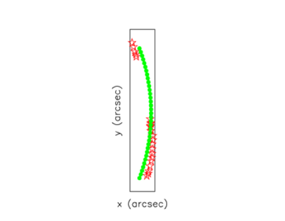
Figure 8: Enlarged view of the three pieces of the giant arc in A2667 (empty red stars) and the theoretical radius (full green points); axes in arcsec.

We can understand the reason for which the giant arc A2267 has a limited angular extension of $\approx~{}31^{\circ}$ by plotting the ratio $\kappa$, equation (37), between the theoretical luminosity as function of $\theta$ and the theoretical luminosity at $\theta=0$ with parameters as in Table 4, see Figure 9.

Figure 9: Normalized luminosity as function of the polar angle in deg, parameters as in Table 4

As a practical example at $\approx~{}31^{\circ}/2$, where the factor two arises from the symmetry of the framework, the theoretical luminosity is decreased of a factor $\kappa=0.987$ in respect to the value at $\theta=0$. We now introduce the threshold luminosity, $L_{tr}$, which is an observational parameter. The theoretical luminosity will scale as function of the polar angle as $L_{theo}(\theta)\propto L_{0}*r$ where $L_{0}$ is the theoretical luminosity at $\theta=0$ and $\kappa$ has been defined in equation (37). When the inequality $L_{theo}<L_{tr}$ is verified the giant arc is impossible to detect and only the zone characterized by low values of the polar angle will be detected.

In our model the velocity with parameters as in Table 4 is function of the polar angle, see Figure 10, and has range $37~{}km/s\,<\,v(\theta)\,<\,142\,km/s$. As a comparison a velocity $50~{}km/s\,<\,v\,<\,75\,km/s$ is measured in A2267, see Figure 5 in [36].

Figure 10: Velocity in km/s as function of the polar angle in deg.

5.2 Simulation of many giants arcs

The presence of multiple giants arcs in the CLASH cluster, see as an example Figure 11 in [28], can be simulated adopting the following steps

• A given number of SBs, as an example 15, are generated with variable lifetime, $t$, see Figure 11

• For each SB we select a section around polar angle equal to zero characterized by a fixed angle of $\approx~{}31^{\circ}$ and we randomly rotate it around the origin, see Figure 12

• The centers of the SBs are randomly placed in a squared box with side of 300 kpc, see Figure 13

Figure 11: Multiple sections of the SB with time,$t$ comprised in $[10^{6}~{}yr,~{}10^{8}~{}yr]$ and other parameters as in Table 4.

Figure 12: Multiple sections of the SB as in Figure 11 with angular extension of the polar angle, $\theta$, of $\approx~{}31^{\circ}$ and progressive rotation of the selected piece of section.

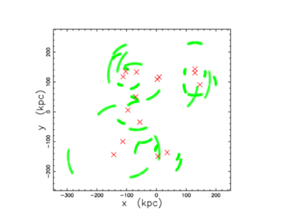
Figure 13: Multiple sections of SB as in Figure 12 with random shift of the origin of the selected SB (green empty stars). The random shift denotes the galaxies (red crosses).

Table 5 reports the theoretical statistical parameters of the above simulation for the radial distance from the arc center to the cluster center in kpc. A comparison should be done with the astronomical parameters for the CLASH clusters of Table 1.

Table 5: Statistical parameters of the radial distance from the theoretical arc center to the cluster center in kpc

50

165

349

6 Theory of the image

We now review the theory of the image for the case of optically thin medium both from an analytical and an analytical point of view.

6.1 The elliptical shell

A real ellipsoid represents a first approximation of the asymmetric giants arcs and has equation

$$\frac{z^{2}}{a^{2}}+\frac{x^{2}}{b^{2}}+\frac{y^{2}}{d^{2}}=1\quad,$$ (43)

in which the polar axis is the z-axis.

We are interested in the section of the ellipsoid $y=0$ which is defined by the following external ellipse

$$\frac{z^{2}}{a^{2}}+\frac{x^{2}}{b^{2}}=1\quad.$$ (44)

We assume that the emission takes place in a thin layer comprised between the external ellipse and the internal ellipse defined by

$$\frac{z^{2}}{(a-c)^{2}}+\frac{x^{2}}{(b-c)^{2}}=1\quad,$$ (45)

see Figure 14.

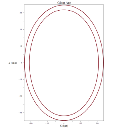
Figure 14: Internal and external ellipses when $a=347\,kpc$,$b=237\,kpc$ and $c=\frac{a}{12}\,kpc$.

We therefore assume that the number density $C$ is constant and in particular rises from 0 at (0,a) to a maximum value $C_{m}$, remains constant up to (0,a-c) and then falls again to 0. The length of sight, when the observer is situated at the infinity of the $x$-axis, is the locus parallel to the $x$-axis which crosses the position $z$ in a Cartesian $x-z$ plane and terminates at the external ellipse. The locus length is

$$l_{I}=2\,{\frac{\sqrt{{a}^{2}-{z}^{2}}b}{a}}$$ (46)

$$when\quad(a-c)\leq z<a$$

$$l_{II}=2\,{\frac{\sqrt{{a}^{2}-{z}^{2}}b}{a}}-2\,{\frac{\sqrt{{a}^{2}-2\,ac+{c}^{2}-{z}^{2}}\left(b-c\right)}{a-c}}$$ (47)

$$when\quad 0\leq z<(a-c)\quad.$$

In the case of optically thin medium, the intensity is split in two cases

$$I_{I}(z;a,b)=I_{m}\times 2\,{\frac{\sqrt{{a}^{2}-{z}^{2}}b}{a}}$$ (48)

$$when\quad(a-c)\leq z<a$$

$$I_{II}(z;a,,c)=$$

$$I_{m}\times\Big{(}2\,{\frac{\sqrt{{a}^{2}-{z}^{2}}b}{a}}-2\,{\frac{\sqrt{{a}^{2}-2\,ac+{c}^{2}-{z}^{2}}\left(b-c\right)}{a-c}}\Big{)}$$ (49)

$$when\quad 0\leq z<(a-c)\quad,$$

where $I_{m}$ is a constant which allows to compare the theoretical intensity with the observed one. A typical profile in intensity along the z-axis is reported in Figure 15.

Figure 15: The intensity profile along the z-axis when when $a=347\,kpc$,$b=237\,kpc$ $c=\frac{a}{12}\,kpc$ and $I_{m}$=1.

The ratio, $\kappa$, between the theoretical intensity at the maximum, $(z=a-c)$, and at the minimum, ($z=0$), is given by

$$\frac{I_{I}(z=a-c)}{I_{II}(z=0)}=\kappa={\frac{\sqrt{2\,a-c}b}{\sqrt{c}a}}\quad.$$ (50)

As an example the values $a=6\,kpc$,$b=4\,kpc$, $c=\frac{a}{12}\,kpc$ gives $\kappa=3.19$. The knowledge of the above ratio from the observations allows to deduce $c$ once $a$ and $b$ are given by the observed morphology

$$c=2\,{\frac{a{b}^{2}}{{a}^{2}{r}^{2}+{b}^{2}}}\quad.$$ (51)

The above analytical model explains the hole in luminosity visible in the astrophysical shells such as supernovae and SBs. More details can be found in [40].

6.2 The numerical shell

The source of luminosity is assumed here to be the flux of kinetic energy, $L_{m}$,

$$L_{m}=\frac{1}{2}\rho AV^{3}\quad,$$ (52)

where $A$ is the considered area, $V$ is the velocity and $\rho$ is the density. In our case $A=r^{2}\Delta\Omega$, where $\Delta\Omega$ is the considered solid angle and $r(\theta)$ the temporary radius along the chosen direction . The observed luminosity along a given direction can be expressed as

$$L=\epsilon L_{m}\quad,$$ (53)

where $\epsilon$ is a constant of conversion from the mechanical luminosity to the observed luminosity.

We review the algorithm that allows to build the image, see [41]:

• An empty memory grid ${\mathcal{M}}(i,j,k)$ which contains $NDIM^{3}$ pixels is considered

• We first generate an internal 3D surface of revolution by rotating the ideal image of $360^{\circ}$ around the polar direction and a second external surface of revolution at a fixed distance $\Delta R$ from the first surface. As an example, we fixed $\Delta R=R/12$, where $R$ is the momentary radius of expansion. The points on the memory grid which lie between the internal and external surfaces are memorized on ${\mathcal{M}}(i,j,k)$ by a variable integer number according to formula (52) and density $\rho$ proportional to the swept mass.

• Each point of ${\mathcal{M}}(i,j,k)$ has spatial coordinates $x,y,z$ which can be represented by the following $1\times 3$ matrix, $A$,

  $$A=\left[\begin{array}[]{c}x\\ \vskip 6.0pt plus 2.0pt minus 2.0pt\cr y\\ \vskip 6.0pt plus 2.0pt minus 2.0pt\cr{\it z}\end{array}\right]\quad.$$ (54)

  The orientation of the object is characterized by the Euler angles $(\Phi,\Theta,\Psi)$ and therefore by a total $3\times 3$ rotation matrix, $E$. The matrix point is represented by the following $1\times 3$ matrix, $B$,

  $$B=E\cdot A\quad.$$ (55)

• The intensity map is obtained by summing the points of the rotated images along a particular direction.

The image of A2267 built with the above algorithm is shown in Figure 16.

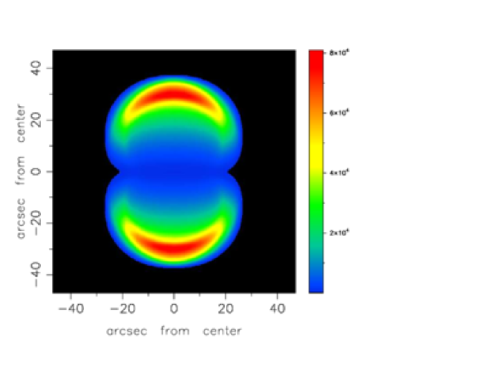
Figure 16: Contour map of ${\it I}$ for A2267, the $x$ and $y$ axes are in $arcsec$. The three Euler angles characterizing the orientation are $\Phi$=0^∘, $\Theta$=90 ^∘ and $\Psi$=90 ^∘, and NDIM=400.

The threshold intensity, $I_{tr}$, is

$$I_{max}\,\kappa=I_{max}\quad,$$ (56)

where $I_{max}$, is the maximum value of intensity characterizing the ring and $\kappa$ is a parameter which allows matching theory with observations and was previously defined in equation (37). A typical image with a hole is visible in Figure 17.

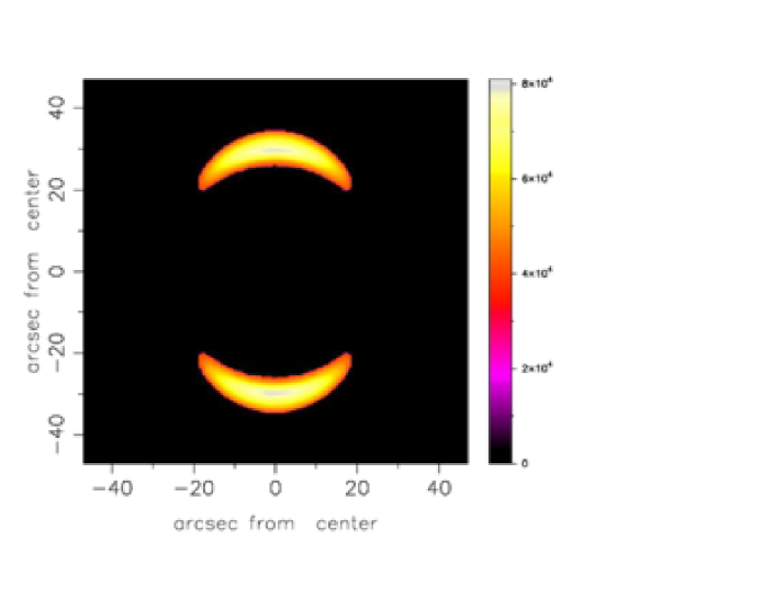
Figure 17: The same as Figure 16 parameters as in Figure 16 and $\kappa=0.5$.

The opening angle of the visible arc can be parametrized as function of the ratio $\kappa$, see Figure 18. An opening of $\approx~{}31^{\circ}$ is reached at $\kappa\approx 0.95$.

Figure 18: The opening angle of the visible simulated arc as function of $\kappa$; parameters as in Figure 16.

7 Conclusions

The equation of motion

The giants arcs are connected with the visible part of the SBs which advance in the intracluster medium surrounding the host galaxies. The chosen profile of density is hyperbolic, see equation (10), and the momentum conservation along a given direction allows to derive the equation of motion as function of the polar angle, see equation (3.2). The image

According to the theory here presented the giants arcs are the visible part of an advancing SB. An analytical explanation for the limited angular extent of the giant arcs is represented by the theoretical luminosity as function of the polar angle, see equation (37). An increase in the polar angle produces a decrease of the theoretical luminosity and the arc becomes invisible. Selecting a given numbers of SBs with variable lifetime and randomly inserting them in a cubic box of side $\approx~{}600\,kpc$ is possible to simulate the giants arcs visible in the clusters of galaxies, see Figure 13 and relative statistical parameters in Table 5.

References

- [1] Lynds R and Petrosian V 1986 Giant Luminous Arcs in Galaxy Clusters in Bulletin of the American Astronomical Society vol 18 of Bulletin of the American Astronomical Society p 1014
- [2] Paczynski B 1987 Giant luminous arcs discovered in two clusters of galaxies Nature 325, 572
- [3] Soucail G, Fort B, Mellier Y and Picat J 1987 A blue ring-like structure, in the center of the a 370 cluster of galaxies Astronomy and Astrophysics 172, L14
- [4] Kovner I 1987 Giant luminous arcs from gravitational lensing Nature 327, 193
- [5] Waldrop M M 1987 The Giant Arcs are Gravitational Mirages Science 238, 1351
- [6] Soucail G, Mellier Y, Fort B, Mathez G and Cailloux M 1988 The giant arc in A 370 - Spectroscopic evidence for gravitational lensing from a source at Z = 0.724 A&A 191, L19
- [7] Narasimha D and Chitre S M 1988 Giant Luminous Arcs in Galaxy Clusters ApJ 332, 75
- [8] Kaufmann R and Straumann N 2000 Giant Arc Statistics and Cosmological Parameters Annalen der Physik 512, 384 (Preprint %****␣ms.tex␣Line␣1600␣****astro-ph/9911037)
- [9] Wambsganss J, Bode P and Ostriker J P 2004 Giant Arc Statistics in Concord with a Concordance Lambda Cold Dark Matter Universe ApJ 606, L93 (Preprint astro-ph/0306088)
- [10] Dalal N, Holder G and Hennawi J F 2004 Statistics of Giant Arcs in Galaxy Clusters ApJ 609, 50 (Preprint astro-ph/0310306)
- [11] Li G L, Mao S, Jing Y P, Mo H J, Gao L and Lin W P 2006 The giant arc statistics in the three-year Wilkinson Microwave Anisotropy Probe cosmological model MNRAS 372, L73 (Preprint astro-ph/0608192)
- [12] Wambsganss J, Ostriker J P and Bode P 2008 The Effect of Baryon Cooling on the Statistics of Giant Arcs and Multiple Quasars ApJ 676, 753 (Preprint 0707.1482)
- [13] Bayliss M B 2012 Broadband Photometry of 105 Giant Arcs: Redshift Constraints and Implications for Giant Arc Statistics ApJ 744 156
- [14] Hammer F and Rigaut F 1989 Giant luminous arcs from lensing - Determination of the mass distribution inside distant cluster cores A&A 226, 45
- [15] Wu X P and Mao S 1996 The Cosmological Constant and Statistical Lensing of Giant Arcs ApJ 463, 404 (Preprint astro-ph/9512014)
- [16] Lewis G F 2001 Gravitational Microlensing of Giant Luminous Arcs: a Test for Compact Dark Matter in Clusters of Galaxies PASA 18, 182
- [17] Mahdi H S, van Beek M, Elahi P J, Lewis G F, Power C and Killedar M 2014 Gravitational lensing in WDM cosmologies: the cross-section for giant arcs MNRAS 441, 1954 (Preprint 1404.1644)
- [18] Dekel A and Braun E 1988 Giant Arcs-Spherical Shells ? in J Audouze, M C Pelletan, A Szalay, Y B Zel’dovich and P J E Peebles, eds, Large Scale Structures of the Universe vol 130 of IAU Symposium p 598
- [19] Braun E and Dekel A 1988 On the giant arcs in clusters of galaxies - Can they be shells? Comments on Astrophysics 12, 233
- [20] Efremov Y N, Elmegreen B G and Hodge P W 1998 Giant Shells and Stellar Arcs as Relics of Gamma-Ray Burst Explosions ApJ 501, L163 (Preprint astro-ph/9805236)
- [21] Zaninetti L 2017 The ring produced by an extra-galactic superbubble in flat cosmology Journal of High Energy Physics, Gravitation and Cosmology 3, 339
- [22] Zaninetti L 2016 Pade approximant and minimax rational approximation in standard cosmology Galaxies 4(1), 4 ISSN 2075-4434 URL http://www.mdpi.com/2075-4434/4/1/4
- [23] Suzuki N, Rubin D, Lidman C, Aldering G, Amanullah R, Barbary K and Barrientos L F 2012 The Hubble Space Telescope Cluster Supernova Survey. V. Improving the Dark-energy Constraints above z greater than 1 and Building an Early-type-hosted Supernova Sample ApJ 746 85
- [24] Zaninetti L 2015 On the Number of Galaxies at High Redshift Galaxies 3, 129
- [25] Peebles P J E 1993 Principles of Physical Cosmology (Princeton, N.J.: Princeton University Press)
- [26] McCray R A 1987 Coronal interstellar gas and supernova remnants in A Dalgarno & D Layzer, ed, Spectroscopy of Astrophysical Plasmas (Cambridge, UK: Cambridge University Press) pp 255–278
- [27] Zaninetti L 2018 The physics of asymmetric supernovae and supernovae remnants Applied Physics Research 6, 25
- [28] Xu B, Postman M, Meneghetti M, Seitz S, Zitrin A, Merten J, Maoz D, Frye B, Umetsu K, Zheng W, Bradley L, Vega J and Koekemoer A 2016 The Detection and Statistics of Giant Arcs behind CLASH Clusters ApJ 817 85 (Preprint 1511.04002)
- [29] Eales S, Dunne L, Clements D and Cooray A 2010 The Herschel ATLAS PASP 122, 499 (Preprint 0910.4279)
- [30] Tamura Y, Oguri M, Iono D, Hatsukade B, Matsuda Y and Hayashi M 2015 High-resolution ALMA observations of SDP.81. I. The innermost mass profile of the lensing elliptical galaxy probed by 30 milli-arcsecond images PASJ 67 72 (Preprint 1503.07605)
- [31] ALMA Partnership, Vlahakis C, Hunter T R and Hodge J A 2015 The 2014 ALMA Long Baseline Campaign: Observations of the Strongly Lensed Submillimeter Galaxy HATLAS J090311.6+003906 at z = 3.042 ApJ 808 L4 (Preprint 1503.02652)
- [32] Rybak M, Vegetti S, McKean J P, Andreani P and White S D M 2015 ALMA imaging of SDP.81 - II. A pixelated reconstruction of the CO emission lines MNRAS 453, L26 (Preprint 1506.01425)
- [33] Hatsukade B, Tamura Y, Iono D, Matsuda Y, Hayashi M and Oguri M 2015 High-resolution ALMA observations of SDP.81. II. Molecular clump properties of a lensed submillimeter galaxy at z = 3.042 PASJ 67 93 (Preprint 1503.07997)
- [34] Wong K C, Suyu S H and Matsushita S 2015 The Innermost Mass Distribution of the Gravitational Lens SDP.81 from ALMA Observations ApJ 811 115 (Preprint 1503.05558)
- [35] Hezaveh Y D, Dalal N and Marrone D P 2016 Detection of Lensing Substructure Using ALMA Observations of the Dusty Galaxy SDP.81 ApJ 823 37 (Preprint 1601.01388)
- [36] Yuan T T, Kewley L J, Swinbank A M and Richard J 2012 The A2667 Giant Arc at z = 1.03: Evidence for Large-Scale Shocks at High Redshift ApJ 759 66 (Preprint 1209.3805)
- [37] Dyson, J E and Williams, D A 1997 The physics of the interstellar medium (Bristol: Institute of Physics Publishing)
- [38] McCray R and Kafatos M 1987 Supershells and propagating star formation ApJ 317, 190
- [39] Zaninetti L 2004 On the Shape of Superbubbles Evolving in the Galactic Plane PASJ 56, 1067
- [40] Zaninetti L 2018 The Fermi Bubbles as a Superbubble International Journal of Astronomy and Astrophysics 8, 200 (Preprint 1806.09092)
- [41] Zaninetti L 2013 Three dimensional evolution of sn 1987a in a self-gravitating disk International Journal of Astronomy and Astrophysics 3, 93