Testing the $f(R)$-theory of gravity

Abstract

A procedure of testing the $f(R)$-theory of gravity is discussed. The latter is an extension of the general theory of relativity (GR). In order this extended theory (in some variant) to be really confirmed as a more precise theory it must be tested. To do that we first have to solve an equation generalizing Einstein’s equation in the GR. However, solving this generalized Einstein’s equation is often very hard, even it is impossible in general to find an exact solution. It is why the perturbation method for solving this equation is used. In a recent work [1] a perturbation method was applied to the $f(R)$-theory of gravity in a central gravitational field which is a good approximation in many circumstances. There, perturbative solutions were found for a general form and some special forms of $f(R)$. These solutions may allow us to test an $f(R)$-theory of gravity by calculating some quantities which can be verified later by the experiment (observation). In [1] an illustration was made on the case $f(R)=R+\lambda R^{2}$. For this case, in the present article, the orbital precession of S2 orbiting around Sgr A* is calculated in a higher-order of approximation. The $f(R)$-theory of gravity should be also tested for other variants of $f(R)$ not considered yet in [1]. Here, several representative variants are considered and in each case the orbital precession is calculated for the Sun–Mercury- and the Sgr A*–S2 gravitational systems so that it can be compared with the value observed by a (future) experiment. Following the same method of [1] a light bending angle for an $f(R)$ model in a central gravitational field can be also calculated and it could be a useful exercise.

1 Introduction

The General theory of Relativity (GR) is one of the greatest theories of the 20th century. The heart of the GR is Einstein’s equation [2, 3, 4]

$$R^{\mu}_{~{}\nu}-\frac{1}{2}R\delta^{\mu}_{~{}\nu}=-\frac{8\pi{G}}{c^{4}}T^{\mu}_{~{}\nu},$$ (1)

derived from the Lagrangian (Lagrangian density)

$$L_{G}=R,$$ (2)

where $T^{\mu}_{~{}\nu}$ is the enery-momentum tensor of the matter. This theory can explain and predict many gravitational phenomena (of the normal matter) in the Universe. Remarkably, recent detections of gravitational waves by the LIGO and Vigro collaborations (see, for instance, [5, 6]) proved once again the predictive power of the GR. If the latter can excellently describe gravitational phenomena of the normal matter, it is not, however, a good theory for explanation of a number of other phenomena such as dark matter, dark energy, cosmic inflation, etc., as well as it cannot accommodate quantum gravity. Various models and theories have been suggested to solve these problems. For example, for solving the dark energy problem, one of the first and simplest attempts is to add a cosmological constant $\Lambda$ to the Lagrangian (2), becoming $L^{\Lambda}_{G}=R-2\Lambda$. This theory has, however, its own problems (see, for example, [7, 8, 9] for more details).

One more general but still relatively simple theory, expected to solve a wider range of problems in cosmology, is the so-called $f(R)$-theory of gravity (or just $f(R)$-theory or $f(R)$-gravity for short) in which Lagrangian (2) is replaced by

$${\cal L}_{G}=f(R),$$ (3)

which is a scalar function of the scalar curvature $R$. Thus, Einstein’s equation must be replaced by the equation [8, 9, 10]

$$f^{\prime}(R)R^{\mu}_{~{}\nu}-\delta^{\mu}_{~{}\nu}\square f^{\prime}(R)+\nabla^{\mu}\nabla_{\nu}f^{\prime}(R)-\frac{1}{2}f(R)\delta^{\mu}_{~{}\nu}=-kT^{\mu}_{~{}\nu},$$ (4)

where $k=\frac{8\pi G}{c^{4}}$, $\square=\nabla_{\mu}\nabla^{\mu}$ with $\nabla_{\mu}$ being a covariant derivative and $f^{\prime}(R)=\frac{df(R)}{dR}$. Presently, the $f(R)$-theory is one of the hotest topics in cosmology with different versions of $f(R)$ considered (for review, see, for example, [8] – [26]) such as those with $f(R)=R+\lambda R^{2}$ or $f(R)=R-\frac{\lambda}{R^{n}}$, etc. However, to solve Eq. (4), especially, for an exact solution, is usually very difficult, even impossible. To get rid of this situation, some approximation conditions are sometimes required so that approximate solutions can be found. Among such conditions the spherical symmetry which is a quite good approximation in many cases is often chosen. Following this strategy in a recent work [1] we solved Eq. (4) for a general $f(R)$-theory in a central (gravitational) field which in general is not static, and obtained approximate solutions in vacuum and in the presence of matter. Then, as a test and illustration, applications of these solutions for $f(R)=R+\lambda R^{2}$ are presented. In the present paper we continue testing other versions of the $f(R)$-theory. Before doing that in Sect. 3, we will briefly recall in the next section some results of [1] to make this paper more self-contained. Some conclusions and comments are given in the last section, Sect. 4. Here, for convenience, we keep the conventions used in [1].

2 Perturbative solutions of the $f(R)$-theory in a central field

Let us summarize some results obtained in [1]. As the GR is a very precise theory, it is reasonable to assume that a realistic $f(R)$ theory differs just slightly from the GR, that is, $f(R)$ can be written in the form

$$f(R)=R+\lambda h(R),$$ (5)

where $\lambda$ is a parameter and $h(R)$ is a scalar function of $R$ such that $\lambda h(R)$ and its derivatives are very small quantities in comparison with $R$. With $f(R)$ given in (5) the modified Einstein’s equation (4) becomes

$$R^{\mu}_{~{}\nu}-\frac{1}{2}\delta^{\mu}_{~{}\nu}R+\lambda h^{\prime}(R)R^{\mu}_{~{}\nu}-\frac{\lambda}{2}\delta^{\mu}_{~{}\nu}h(R)-\lambda\delta^{\mu}_{~{}\nu}\square h^{\prime}(R)+\lambda\nabla^{\mu}\nabla_{\nu}h^{\prime}(R)=-kT^{\mu}_{~{}\nu}.$$ (6)

Solving this equation for a central field of a gravitational source of mass $M$ we obtain a Schwarzschild-type solution ($x^{0}=ct$)

$$ds^{2}=\left[1-\frac{2GM_{f}(t)}{c^{2}r}\right]{dx^{0}}^{2}-\frac{dr^{2}}{1-\frac{2GM_{f}(t)}{c^{2}r}}-r^{2}(d\theta^{2}+\sin^{2}\theta{d\varphi^{2}})$$ (7)

with

$$M_{f}(t)=M-\lambda M_{1}(t)-\lambda M_{2}(t),$$ (8)

treated as an effective mass, which in general is a function of time, even for a constant $M$, where

$$\lambda M_{1}(t)=\frac{2\pi\lambda[R_{0}(t)]^{3}}{3kc^{2}}\left[h(kT^{0}_{~{}0})+kT^{0}_{~{}0}h^{\prime}(kT^{0}_{~{}0})\right],$$ (9)

$$\lambda M_{2}(t)=\frac{4\pi\lambda}{kc^{2}}h^{\prime\prime}(kT^{0}_{~{}0})\left[\frac{\partial}{\partial t}\frac{M}{[R_{0}(t)]^{3}}\right]^{2}~{}\alpha(t),$$ (10)

$$T^{0}_{~{}0}={Mc^{2}\over{\frac{4}{3}}\pi{[R_{0}(t)]}^{3}},$$ (11)

$$\alpha(t)=~{} \frac{3k^{2}c^{2}R_{0}(t)}{256\pi^{2}[\xi(t)]^{4}}\left\{\frac{3}{\xi(t)R_{0}(t)}\arcsin[\xi(t)R_{0}(t)]-\left(3+2[\xi(t)R_{0}(t)]^{2}\right)\sqrt{1-[\xi(t)R_{0}(t)]^{2}}\right\}$$

$$\times\left(1-[\xi(t)R_{0}(t)]^{2}\right)^{-3/2},$$ (12)

and

$$\xi^{2}(t)=\frac{kMc^{2}}{4\pi[R_{0}(t)]^{3}}.$$ (13)

Above, the radius of the considered body-gravitational source $R_{0}$ is also a function of time, $R_{0}=R_{0}(t)$, in general. If the body-gravitational source shrinks or expands (it means that its radius varies with time), the metric would depend on time. This affect does not happen in the GR and may lead to new phenomena which is a subject of our current research.

Applying the solution (7) to the problem of a planet orbiting around an isotropic star of mass $M$ we find the equation of motion

$$\frac{l^{2}(t)}{m\beta(t)r}=1+\sqrt{1+\frac{2E(t)l^{2}(t)}{m\beta^{2}(t)}}\mbox{cos}\left(\sqrt{1-\frac{6m^{2}G^{2}M_{f}^{2}(t)}{c^{2}\mu^{2}}}\varphi\right),$$ (14)

with $r$ and $\varphi$ being polar coordinates of the planet in a frame with origin at the star’s center, while

$$\beta(t)=~{} mGM_{f}(t)\left[1+\frac{4E(t)}{mc^{2}}\right],$$ (15)

$$l^{2}(t)=~{} \mu^{2}\left[1-\frac{6m^{2}G^{2}M_{f}^{2}(t)}{c^{2}\mu^{2}}\right],$$ (16)

where $E(t)$ is the energy of the planet (subtracted by the rest energy $mc^{2}$) in the gravitational field, and $\mu$ is the angular momentum (which is conserved). The orbit described by (14) is nearly-elliptic with parameters, such as major and minor axes, changing with time if the central field is not static (even when the total mass $M$ is constant, as, for example, in the case of a start expanding or collapsing but keeping its isotropic form). Following [1] we can calculate the minimal value $r_{p}$ and the maximal value $r_{a}$ of $r$

$$r_{p/a}= \frac{l^{2}(t_{e})}{m\beta(t_{e})\pm\sqrt{m^{2}\beta^{2}(t_{e})+2mE(t_{n})l^{2}(t_{e})}},$$ (17)

where the signs plus and minus are for $r_{p}$ and $r_{a}$, respectively, and $t_{e}$ is the time at the extremum $r_{e}$ being $r_{p}$ or $r_{a}$. The orbital precession can be also calculated

$$\Delta\varphi_{e}(k)=\frac{6\pi m^{2}G^{2}M_{f}^{2}(t_{k})}{c^{2}\mu^{2}}.$$ (18)

The latter differs from Einstein’s precession by a correction which at the first order of perturbation reads

$$\delta\varphi_{e}(k)\cong\frac{-12\pi m^{2}G^{2}\lambda M[M_{1}(t_{k})+M_{2}(t_{k})]}{c^{2}\mu^{2}},$$ (19)

where $t_{k}$ ($k=1,2,3,...$) is the time when the planet passes the extremum points $r_{k}$, which are either $r_{p}$ or $r_{a}$ (but not both). If the central field is static, $\Delta\varphi_{e}$ (therefore, $\delta\varphi_{e}$) remains always constant (see Figure 1 for illustration),

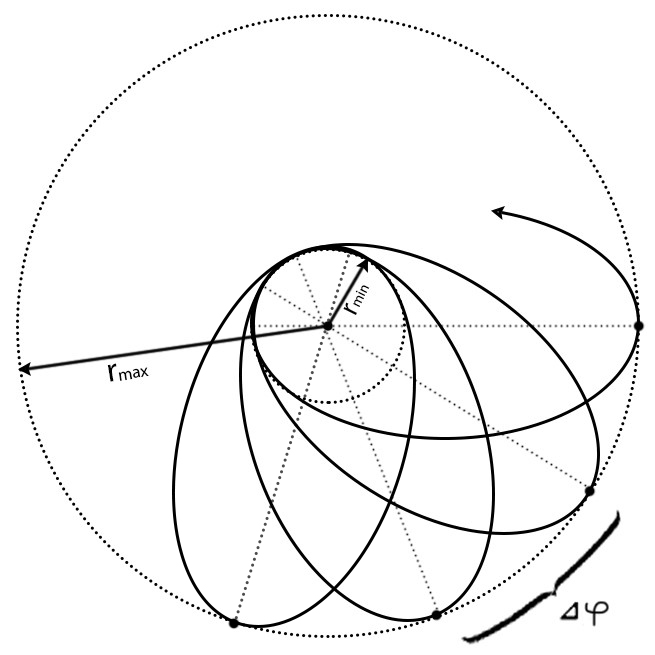
Figure 1: In a static central field, both $r_{p/a}$ and $\Delta\varphi$ remain constant as in the GR but differ from the corresponding Einstein’s values by constant corrections[1].

but when the central field is not static, $\Delta\varphi_{e}$ (therefore, $\delta\varphi_{e}$) may change with time.

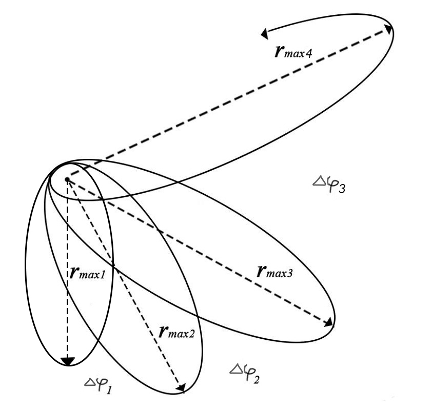
Figure 2: In a non-static case, both $r_{p/a}$ and $\Delta\varphi$ in general vary with time, unlike in the GR they remain always constant in a central field (if the source has a constant mass) [1].

There is not only a correction (18) to the orbital precession, but, as seen from (17), the orbital axes also change with time (for illustration, see Figure 2). They are new effects compared with the GR and require to be tested. In [1] testing the $f(R)$-theory was illustrated with $f(R)=R+\lambda R^{2}$, here, in this paper, we will do that with other variants.

3 Testing the $f(R)$-theory in some variants

For simplicity, let us consider an $f(R)$-theory in a static central field. As seen before, our perturbative solution looks like a Schwarzschild solution in the GR with the original mass $M$ replaced by an effective mass $M_{f}=M-\lambda M_{1}-\lambda M_{2}$ which now is just $M_{f}=M-\lambda M_{1}$ because $M_{2}=0$ for a static field. Then, from (18) we have

$$\Delta\varphi_{f(R)}=\frac{6\pi G^{2}m^{2}M_{f}^{2}}{c^{2}\mu^{2}}=\frac{6\pi G^{2}m^{2}(M-\lambda M_{1})^{2}}{c^{2}\mu^{2}}.$$ (20)

This latter can be written in the form

$$\Delta\varphi_{f(R)}=\frac{6\pi G(M-\lambda M_{1})}{c^{2}a(1-e^{2})},$$ (21)

where

$$\frac{\mu^{2}}{GM_{f}m^{2}}=a(1-e^{2})$$ (22)

is used, with $a$ being the length of a semi-major axis and $e$ being the eccentricity of an orbital ellipse [3], hence

$$\lambda M_{1}=M-\frac{c^{2}a(1-e^{2})}{6\pi G}\Delta\varphi_{f(R)}.$$ (23)

It is worth noting that this formula, valid for any (well-defined) $f(R)$, not only for $f(R)=R+\lambda R^{2}$, is different from (149) in [1] because it is calculated in a higher order of precision by using in (22) the effective mass $M_{f}=M-\lambda M_{1}$ instead of the ”bare” mass $M$ used in [1]. The value of $\lambda M_{1}$ is the same for an arbitrary $f(R)$ but $M_{1}$, thus $\lambda$, is different for different $f(R)$. Next, using the following data [27]:

$$c=299792458m/s;$$

$$G=6.67259\times 10^{-11}kg^{-1}m^{3}s^{-2};$$

$$\frac{2GM}{c^{2}}=2.95325008\times 10^{3}m;$$

$$k=\frac{8\pi G}{c^{4}}=2.0761154\times 10^{-43}kg^{-1}m^{-1}s^{2};$$ (24)

$$M=1.988919\times 10^{30}kg;$$

$$a=5.7909175\times 10^{10}m;$$

$$e=0.20563069;$$

$$\Delta\varphi_{obs}=2\pi(7.98734\pm 0,00037)\times 10^{-8}~{}radian/revolution,$$

we obtain the deviation between the observed value and the GR value of the Mercury’s orbital precession

$$\Delta\varphi_{obs}-\Delta\varphi_{GR}=-0.1906\pi\times 10^{-11}radian/revolution.$$ (25)

This deviation may come from the imperfection, though small, of the GR, and suppose it can be explained by the $f(R)$- theory, that is,

$$\Delta\varphi_{f(R)}=\Delta\varphi_{obs}$$ (26)

(upto some smaller errors), or

$$\delta\varphi= ~{}\Delta\varphi_{f(R)}-\Delta\varphi_{GR}=-0.1906\pi\times 10^{-11}radian/revolution.$$ (27)

This requirement can be satisfied if the correction $\lambda M_{1}$ to the mass $M$ equals

$$\lambda M_{1}=23.285244\times 10^{24}kg,$$ (28)

according to (23) and (26). The effective reduction of the Sun’s mass $M=1.988919\times 10^{30}kg$

$$\frac{\lambda M_{1}}{M}=11.707487\times 10^{-6}=0.0011707487~{}\%.$$ (29)

is quite small compared with the Sun’s mass but it may be measurable if a measurement technique precise enough is invented. It is worth noting that the value of $\lambda M_{1}$ is model-independent, i.e., for any well-defined $f(R)$. To estimate $\lambda$ we need, however, a concrete $f(R)$.

Using the perturbation condition $\lambda h(R)\ll R$ for (5) and $R=kT$, where $T=T^{\mu}_{\mu}$, we get

$$\lambda h(kT)\ll kT,$$ (30)

or if $T\approx T^{0}_{~{}0}$, we have

$$\lambda h(kT^{0}_{~{}0})\ll kT^{0}_{~{}0}.$$ (31)

With $T^{0}_{~{}0}=\frac{Mc^{2}}{\frac{4}{3}\pi[R_{0}]^{3}}$ the latter inequation becomes

$$\lambda h(kT^{0}_{~{}0})\ll\frac{6GM}{c^{2}[R_{0}]^{3}}.$$ (32)

From this formula with the Sun’s radius [28]

$$R_{0}\approx 6.957\times 10^{8}m$$ (33)

we see that $\lambda h$ is very small,

$$\lambda h(kT^{0}_{~{}0})\ll 26.3120915\times 10^{-24},$$ (34)

as expected. All results listed above are for an arbitrary $f(R)$. Now let us consider several concrete variants of the $f(R)$-theory.

3.1 Model $f(R)=R+\lambda R^{2}$

This called Starobinsky model [29] was already considered in [1] (more discussions on the meaning of this model can be found in [8]) as model II with $b=2$, but here we reconsider it by doing some calculations at a higher order of precision, namely, as said above, formula (22) with $M_{f}$ replacing $M$ is used instead of $\frac{\mu^{2}}{GMm^{2}}=a(1-e^{2})$ used in [1]. In this model $h(R)=R^{2}$, that is $h(kT^{0}_{~{}0})=[kT^{0}_{~{}0}]^{2}$, and, therefore, due to (11) we have

$$h(kT^{0}_{~{}0})=\left[\frac{kMc^{2}}{\frac{4}{3}\pi[R_{0}]^{3}}\right]^{2},$$ (35)

and

$$kT^{0}_{~{}0}h^{\prime}(kT^{0}_{~{}0})=2\left[\frac{kMc^{2}}{\frac{4}{3}\pi[R_{0}]^{3}}\right]^{2}.$$ (36)

Thus, the perturbation condition (32) for this model imposes an upper bound on $\lambda$:

$$\lambda\ll\frac{c^{2}[R_{0}]^{3}}{6GM}.$$ (37)

Using the data in (24) and (33) we can calculate this bound,

$$\lambda\ll 0.380053\times 10^{23}.$$ (38)

Now inserting (35) and (36) in (9) we write $M_{1}$ in the form

$$M_{1}=\frac{9kc^{2}M^{2}}{8\pi[R_{0}]^{3}},$$ (39)

which, with using (24) and (33) again, gives

$$M_{1}=78.4989\times 10^{6}kg.$$ (40)

From here and (28) we obtain a numerical value of $\lambda$,

$$\lambda=0.296631\times 10^{18}.$$ (41)

The latter is compatible with the perturbation condition (38). The model $f(R)=R+\lambda R^{2}$ with $\lambda$ given in (41) makes a small correction to the GR and fits the observed Mercury’s orbital precession. Now, assuming that the obtained value of $\lambda$ is universal (at least within some range of gravitational field strength) we can predict an orbital precession for another gravitational system. Following this procedure described in more details in [1] and using the data [30]

$$M=4.31\times 10^{6}M_{\odot}=8.57\times 10^{36}kg$$

$$R_{0}=22\times 10^{9}m$$ (42)

$$a=0.123arcsec=14.7\times 10^{13}m$$

$$e=0.88,$$

we can calculate an improved S2 orbital precession $\Delta\varphi^{S2}_{f(R)}$ around SgrA* as

$$\Delta\varphi^{S2}_{f(R)}=1.149305\pi\times 10^{-3}radian/revolution.$$ (43)

This value of $\Delta\varphi^{S2}_{f(R)}$ slightly improves the one calculated in [1] and its deviation from the GR’s value is a bit bigger, thus, more measurable. Now we are moving to other models not considered in details yet in the previous work [1], but we should note first that any function $f(R)$ which can develop a Taylor expansion around $R=0$, coincides at the leading order with $f(R)=R+\lambda R^{2}$.

3.2 Model $f(R)=R+\lambda R^{2}\sum\limits_{n=0}^{+\infty}{a_{n}R^{n}}$

This model is inspired by the Taylor expansion of $f(R)$ considered also in [31, 32] stating that an $f(R)$ theory can be distinguished with the GR only beyond a Kerr solution. Here $a_{n}$ is a coefficient regulating a right dimension of each term $a_{n}R^{n}$, where, $a_{0}$ can be normalized to be 1, $a_{0}=1$. As according to (34)

$$R=kT^{0}_{~{}0}=26.3120915\times 10^{-24}$$ (44)

for the Sun and

$$R=kT^{0}_{~{}0}=35.8523036\times 10^{-22}$$ (45)

for the SgrA*, i.e., $R\ll 1$ in both cases, this model (3.2) is convergent if $a_{n}$ are not very big. As $R\ll 1$ the approximation $f(R)\approx R+\lambda R^{2}$ can be used, and the investigation of this model is similar to that of the previous one (3.1). We classify those models with the same lower-order approximation into one class. The next model also belongs to this class.

3.3 Model $f(R)=Re^{\lambda R}$

Similar to the model considered above, the present model is also inspired by the Taylor expansion of an $f(R)$ for a special choice of coefficients $a_{n}$ (see [33] for another resembling model). One can see from the Taylor series

$$f(R)=Re^{\lambda R}=R\sum\limits_{n=0}^{+\infty}\frac{(\lambda R)^{n}}{n!}=R+\lambda R^{2}+\frac{\lambda^{2}R^{3}}{2}+\frac{\lambda^{3}R^{4}}{3!}+\dotsb$$ (46)

that this model belongs to the same class with the models (3.1) and (3.2). These models describe the same physics, including the same $\lambda$, at the order $R^{2}$ of approximation of $f(R)$. There are other models belonging to this class but we cannot list all here. Of course, if we go to a higher order of approximation we have to do more cumbersome, sometimes, impossible, calculations but the general procedure remains the same. As the correction to the GR is already very small even at the leading order of approximation there is no need at the present to make calculations at the next orders. Therefore, all the $f(R)$ models with $f(R)$ developing a Taylor expansion around $R=0$, describe at the leading order of approximation the same physics as Starobinsky model, that is, they belong to one and the same class referred hereafter to as Starobinsky class. Below we will consider some alternative models, not equivalent to Starobinsky model.

3.4 Model $f(R)=\alpha R^{1+\varepsilon}$

Here $\varepsilon$ is an infinitesimally small number and $\alpha$, which may depend on $\varepsilon$, is a coefficient regulating a right dimension of $f(R)$. To get Einstein’s GR at $\varepsilon=0$ requires $\lim\limits_{\varepsilon\rightarrow 0}\alpha(\varepsilon)=1$. Perturbative solutions of the current model were already considered in [1] but here we suggest a testing procedure. This model for $\varepsilon<0$ (as seen below) does not belong to Starobinsly class as the function $f(R)=\alpha R^{1+\varepsilon}$ cannot develop a Taylor expansion around $R=0$ (but it could belong to a class of a type with a cosmological constant). Now we have

$$\lambda h(R)=\alpha R^{1+\varepsilon}-R,$$ (47)

and, thus,

$$\lambda Rh^{\prime}(R)=(1+\varepsilon)\alpha R^{1+\varepsilon}-R.$$ (48)

Inserting (47) and (48) in (9) we get

$$\lambda M_{1}=-M+\alpha\frac{M}{2}(\varepsilon+2)\left(\frac{3kc^{2}M}{4\pi[R_{o}]^{3}}\right)^{\varepsilon}$$ (49)

and then combining (49) with (28) we obtain the equation

$$-M+\alpha\frac{M}{2}(\varepsilon+2)\left(\frac{3kc^{2}M}{4\pi[R_{o}]^{3}}\right)^{\varepsilon}=23.285244\times 10^{24}.$$ (50)

Using the data from (24) we solve this equation for $\varepsilon$ to get

$$\varepsilon=-2.27364\times 10^{-7},$$ (51)

and from here with (44) and (47) we find $\lambda h(R)=31.1040024\times 10^{-29}$. This value of $\lambda h(R)$ also satisfies the perturbation condition $\lambda h(R)\ll R$. With the value of $\epsilon$ given in (51) we can calculate an orbital precession of Mercury fitting the observed one with the correction (27) to the Einstein value as we did earlier for other models.

In this way we can calculate the orbital precession of S2 orbiting around our Galaxy’s center Sgr A*. Taking (51), (49), (42) and (21) into account we get

$$\Delta\varphi_{f(R)}^{S2}=1.15113\pi\times 10^{-3}radian/revolution,$$ (52)

and the correction to the Einstein value is

$$\delta\varphi^{S2}=\Delta\varphi_{f(R)}^{S2}-\Delta\varphi_{GR}^{S2}=-\pi\times 10^{-8}radian/revolution,$$ (53)

where

$$\Delta\varphi^{S2}_{GR}=1.15114\pi\times 10^{-3}radian/revolution$$ (54)

is the orbital precession calculated by the GR.

3.5 Model $f(R)=R+\lambda\sqrt{R}$

Assuming $\lambda\sqrt{R}\ll R$, the present model is inspired by the model $f(R)=R+\lambda R^{n}$ with $n>0$ (see, for example, [8]). This model does not belong to Starobinsky class (but a class with a cosmological-type constant) either, because $f(R)=R+\lambda\sqrt{R}$ cannot develop a Taylor expansion around $R=0$. In this case

$$h(R)=\sqrt{R},$$ (55)

$$Rh^{\prime}(R)=\frac{\sqrt{R}}{2}.$$ (56)

Now with (55) the perturbation condition (32) becomes

$$\lambda\ll\sqrt{kT^{0}_{~{}0}}=5.129531314\times 10^{-12}.$$ (57)

Inserting (55) and (56) in (9) we obtain the formula

$$M_{1}=\frac{\sqrt{3\pi M}[R_{0}]^{\frac{3}{2}}}{2c\sqrt{k}},$$ (58)

which with (33) and (24) taken into account gives

$$M_{1}=2.908041992\times 10^{41}.$$ (59)

Combining (59) with (28) we get

$$\lambda=8.007189739\times 10^{-17}.$$ (60)

We see that this value of $\lambda$ satisfies the perturbation condition (28) securing the orbital precession of Mercury calculated by the present model fits the observed one, and, therefore, it makes a correction to the Einstein value as given by (27). Following the same procedure we can calculate the orbital precession of S2 around Sgr A*

$$\Delta\varphi_{f(R)}^{S2}=1.15114\pi\times 10^{-3}radian/revolution,$$ (61)

which is (almost) the same as the value (54) obtained by the GR.

4 Conclusions

The general theory of relativity is very successful theory which is the foundation of the modern cosmology, but it cannot solve a number of problems like those of dark matter, dark energy, inflation, quantum gravity, etc., that require a modification or an extension of this theory. The so-called $f(R)$-theory of gravity is one of the most popular and simplest modified theories of gravity generalizing the GR in order to resolve difficulties of the latter. As any other new theory the $f(R)$-theory must be verified by the experiment (observation). One of the ways to do that is to compare some theoretically derived quantities with the corresponding measured (observed) ones. Therefore, we have to prepare theoretical samples to be checked later experimentally. In the present article, using the method of [1] we have calculated for several representative variants of the $f(R)$-theory orbital precessions, which should be compared with the available measured values. Following [1] it is not difficult to calculate a light bending angle for an $f(R)$ model in a central gravitational field, but here we have calculated orbital precessions as examples and leave the calculations on the light bending as an exercise for those interested. We hope a precision measurement of these quantities can be organized in a not very far future. For conclusion, we have considered for testing several variants of the $f(R)$-gravity, but so far, before having experimental/observation data, we cannot compare them in order to say which is a better, i.e., more realistic, model. However, we can state that the orbital precessions calculated by the models of the class III.1 – III.3 deviate more from the GR than those for III.4 and III.5, thus, the former are easier to be experimentally tested. Some of the above considered models have found physical interpretations (to be verified experimentally) but other ones suggested just as alternative possibilities within a mathematical completion may find later physical interpretations.

References

- [1] Nguyen Anh Ky, Pham Van Ky and Nguyen Thi Hong Van, Eur. Phys. J. C 78 (2018) no. 7 539.
- [2] S. Weinberg, Gravitation and cosmology: Principles and applications of the general theory of relativity, John Wiley Son, New York, 1972.
- [3] L. D. Landau and E. M. Lifshitz, The classical theory of fields, vol. 2, Elsevier, Oxford, 1994.
- [4] P. J. E. Peebles, Principles of physical cosmology, Princeton University Press, Princeton, New Jersey, 1993.
- [5] B. P. Abbott et al. [LIGO scientific and Virgo collaborations], Phys. Rev. Lett. 116 (2016) 061102.
- [6] B. P. Abbott et al. [LIGO scientific and Virgo collaborations], Phys. Rev. Lett. 119 (2017) 161101.
- [7] S. Weinberg, Rev. Mod. Phys. 61 (1989) 1-23.
- [8] A. De Felice and S. Tsujikawa, Living Rev. Rel. 13 (2010) 3.
- [9] Thomas P. Sotiriou and Valerio Faraoni, Rev. Mod. Phys. 82 (2010) 451.
- [10] S. Capozziello and M. De Laurentis, Phys. Rept. 509 (2011) 167.
- [11] L. Amendola, D. Polarski and S. Tsujikawa, Phys. Rev. Lett. 98 (2007) 131302.
- [12] H. Wei, H. Y. Li and X. B. Zou, Nucl. Phys. B 903 (2016) 132.
- [13] L. Amendola, D. Polarski and S. Tsujikawa, Phys. Rev. Lett. 98 (2007) 131302.
- [14] S. Nojiri and S. D. Odintsov, Phys. Rev. D 68 (2003) 123512.
- [15] H. Liu, X. Wang, H. Li and Y. Ma, Eur. Phys. J. C 77 (2017) no. 11 723.
- [16] Z. Amirabi, M. Halilsoy and S. Habib Mazharimousavi, Eur. Phys. J. C 76 (2016) no. 6 338.
- [17] D. Müller, V. C. de Andrade, C. Maia, M. J. Rebouças and A. F. F. Teixeira, Eur. Phys. J. C 75 (2015) no. 1 13.
- [18] T. Multamaki and I. Vilja, Phys. Rev. D 74 (2006) 064022.
- [19] K. Kainulainen, J. Piilonen, V. Reijonen and D. Sunhede, Phys. Rev. D 76 (2007) 024020.
- [20] A. Shojai and F. Shojai, Gen. Rel. Grav. 44 (2012) 211.
- [21] M. Sharif and H. R. Kausar, J. Phys. Soc. Jap. 80 (2011) 044004.
- [22] L. Sebastiani and S. Zerbini, Eur. Phys. J. C 71 (2011) 1591.
- [23] A. L. Erickcek, T. L. Smith and M. Kamionkowski, Phys. Rev. D 74 (2006) 121501.
- [24] E. V. Arbuzova, A. D. Dolgov and L. Reverberi, Astropart. Phys. 54 (2014) 44.
- [25] A. Stabile, Phys. Rev. D 82 (2010) 064021.
- [26] S. Capozziello, A. Stabile and A. Troisi, Mod. Phys. Lett. A 24 (2009) 659.
- [27] B. Majumder, arXiv (2011) 1105.2428v1.
- [28] M. Haberreiter, W. Schmutz and A. G. Kosovichev, Phys. Rev. A 77 (2008) 022107.
- [29] A. A. Starobinsky, Phys. Lett. B 91 (1980) 99.
- [30] S. Gillessen, F. Eisenhauer, S. Trippe, T. Alexander, R. Genzel, F. Martins and T. Ott, Astrophys. J. 692 (2009) 1075.
- [31] D. Psaltis, D. Perrodin, K. R. Dienes and I. Mocioiu, Phys. Rev. Lett. 100 (2008) 091101.
- [32] C. P. L. Berry and J. R. Gair, Phys. Rev. D 83 (2011) 104022.
- [33] E. V. Linder, Phys. Rev. D 80 (2009) 123528.