THE UNIVERSITY OF READING
Department of Mathematics

PhD Thesis

Abstract

In this thesis we study four problems in the area of scattering of time harmonic acoustic or electromagnetic waves by unbounded rough surfaces/unbounded inhomogeneous layers. Specifically the four problems we study are:
i) A boundary value problem for the Helmholtz equation, in both 2 and 3 dimensions, modelling scattering of time harmonic waves due to a source that lies within a finite distance of the boundary and which decays along the boundary, by a layer of spatially varying refractive index above an unbounded rough surface on which the field vanishes. In particular, in the 2D case, the boundary value problem models the scattering of time harmonic electromagnetic waves by an inhomogeneous conducting or dielectric layer above a perfectly conducting unbounded rough surface, with the magnetic permeability a fixed positive constant in the media, in the transverse electric polarization case;
ii) a boundary value problem for the Helmholtz equation with an impedance boundary condition, in 2 and 3 dimensions, modelling the scattering of time harmonic acoustic waves due to a source that lies within a finite distance of the boundary and which decays along the boundary, by an unbounded rough impedance surface;
iii) a problem of scattering of time harmonic waves by a layer of spatially varying refractive index at the interface between semi-infinite half-spaces of fixed positive refractive index (the waves arising due to a source that lies within a finite distance of the layer and which decays along the layer). In the 2D case this models the scattering of time harmonic electromagnetic waves by an infinite inhomogeneous dielectric layer at the interface between semi-infinite homogeneous dielectric half-spaces, with the magnetic permeability a fixed positive constant in the media, in the transverse electric polarization case;
iv) a boundary value problem for the Helmholtz equation with a Dirichlet boundary condition, in 3 dimensions, modelling the scattering of time harmonic acoustic waves due to a point source, by an unbounded, rough, sound soft surface.

We study problems i), ii) and iiii) by variational methods; via analysis of equivalent variational formulations we prove these problems to be well-posed in the following cases: For i) we show that the problem is well-posed for arbitrary rough surfaces that are a finite perturbation of an infinite plane, in the case that the frequency is small or when the medium in the layer has some energy absorption; and when the rough surface is such that the resulting domain has the property that if $x$ is in the domain then so to is every point above $x$, we show the problem to be well-posed for arbitrary large frequency with certain restrictions on the rate of change of the refractive index; for ii) we show that the problem is well-posed for arbitrary rough Lipschitz surfaces that are a finite perturbation of an infinite plane, in the case that the frequency is small; and when the rough surface is the graph of a bounded Lipschitz function, we show the problem to be well-posed for arbitrary frequency; for iii) we establish that the problem is well-posed under certain restrictions on the variation of the index of refraction.

We study problem iv) via a Brakhage-Werner type integral equation formulation, based on an ansatz for the solution as a combined single- and double-layer potential, but replacing the usual fundamental solution of the Helmholtz equation with an appropriate half-space Green’s function. We establish, in the case that the rough surface is the graph of a bounded Lipschitz function, that the problem is well-posed for arbitrary frequency.

An attractive feature of our results is that the bounds we derive, on the inf-sup constants of the sesquilinear forms in problems i), ii) and iii), and on the inverse operator associated with the single- and double-layer potentials in problem iv), are explicit in terms of the index of refraction, the geometry of the scatterer and the other parameters of the respective problems.

Chapter 1 Introduction

1.1 Preamble

Consider, if you will, the following problem: An aeroplane flying above the surface of the earth, generates some noise. This noise travels through the air striking the rough surface of the earth beneath it. The noise bounces off or scatters from the surface. Given that we know the exact nature of the noise produced by the aeroplane, and given that we know the exact shape of the earth’s surface beneath it, can we predict the resultant propagation of noise as it strikes the earth’s surface and scatters?

The above problem is a typical example of what are known as rough surface scattering problems. Rough surface scattering problems arise frequently in the natural world and the study of these problems has been borne out of research in many diverse areas of science. The above example shows their importance to the science of sound propagation and noise control; on a much smaller scale, in the field of nano-technology, they are relevant in the study of the scattering of light from the surface of materials; and in the technology of solar heating, their understanding is important for the correct choice of solar paneling; in addition these problems crop up in medical imaging and seismic exploration.

It is the overall aim then, of the mathematical and engineering community, to resolve these problems. This thesis is intended as a contribution to this subject. We are concerned primarily with the initial, mathematical and theoretical questions that should – to a mathematician at least – be answered, in this field, prior to the implementation of numerical and computational techniques that will simulate the process of rough surface scattering, and ultimately give answers to the problems stated above.

Thus, in what follows, we are concerned with the mathematical aspects of rough surface scattering problems. In particular we are interested in the correct mathematical formulation of these problems and we intend to analyze under which conditions they are well-posed. Specifically we study four rough surface scattering problems. Three of these we study by variational methods – these are acoustic scattering by an impedance surface; electromagnetic scattering by inhomogeneous layers above a perfectly conducting rough surface (the Transverse electric polarization case); and the transmission problem – and one by integral equation methods: acoustic scattering by a sound soft surface. We will shortly take a more precise look at what these problems are and look at the mathematical models that govern acoustic and electromagnetic propagation.

We wish to end this first section by introducing some nomenclature and notation used throughout and by setting the scene of our scattering problems. In accordance with the terminology of the engineering literature, we use the phrase rough surface to denote a surface which is a (usually non-local) perturbation of an infinite plane surface, such that the whole surface lies within a finite distance of the original plane.

Let $x=(x_{1},\dots,x_{n})$ denote a point in $\mathbb{R}^{n}$, $(n=2,3)$, and let $\tilde{x}=(x_{1},\dots,x_{n-1})$ so that $x=(\tilde{x},x_{n})$. Further, for $H\in\mathbb{R}$ let $U_{H}=\{x:x_{n}>H\}$ and $\Gamma_{H}=\{x:x_{n}=H\}$. We will denote the region of space in which the acoustic or electromagnetic waves propagate, i.e. the air above the earth’s surface in the aeroplane problem we described above, as $D$. Thus $D\subset\mathbb{R}^{n}$, and $D$ will be assumed to be a connected open set or domain. Moreover we’ll assume there exist constants $f_{-}<f_{+}$ such that

$$U_{f_{+}}\subset D\subset U_{f_{-}}.$$

We let $\Gamma$ denote the boundary of $D$, i.e. the rough surface. The unit outward normal to $D$ will be denoted $\nu$. Finally, we define $S_{H}:=D\backslash\overline{U_{H}}$.

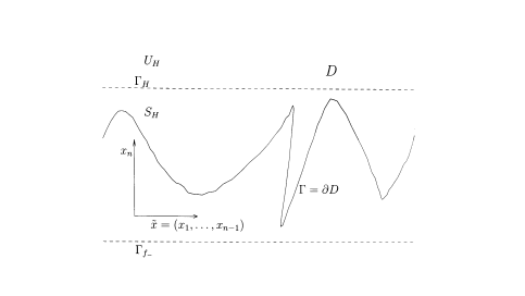
Figure 1.1: Sketch of the geometry.

This definition of $D$ is rather complicated – see the picture below. It may help the reader, in coming to terms with this abstract description to keep in mind the following case, included in our definition of $D$. This is the case where the scattering surface $\Gamma$ is the graph of some bounded continuous function. For example in the 3D case, we have that for a bounded and continuous function $f:\mathbb{R}^{2}\to\mathbb{R}$,

$$\Gamma:=\{x=(x_{1},x_{2},x_{3})\in\mathbb{R}^{3}:x_{3}=f(x_{1},x_{2})\},$$ (1.1)

after which the domain $D$ is given by

$$D=\{x=(x_{1},x_{2},x_{3})\in\mathbb{R}^{3}:x_{3}>f(x_{1},x_{2})\}.$$

Of course, in general one wishes to consider rough surfaces that are not simply the graphs of functions, but of more complex geometry that one encounters in reality. It is a major point of this thesis that we establish well-posedness results for wave scattering by rough surfaces that are not the graphs of functions, under certain other restrictions (low frequency of the waves, for example). Nevertheless a great deal of the well-posedness results we establish in this thesis are restricted to this setting, where the rough surface is the graph of a bounded continuous function.

We aim in the next sections to turn our attention to the mathematical modelling of these problems. We’ll begin by looking at acoustics; then we’ll take a look at electromagnetics.

1.2 The mathematical description of the scattering problems

1.2.1 Acoustics

The wave equation is the classical model that describes acoustic propagation. Let $U(x,t):D\times\mathbb{R}\to\mathbb{C}$ denote the perturbation of pressure at a point $x$ in $D$ and at a time $t>0$. It is this that we seek to find. In other words, for example, it represents the resultant sound distribution that we desired to predict in the aeroplane example earlier. Let $G(x,t):D\times\mathbb{R}\to\mathbb{C}$ denote the source of acoustic disturbance, i.e. the noise produced by the aeroplane, which we suppose we know or are given. Then the inhomogeneous wave equation relates the two via,

$$\frac{1}{c^{2}}\frac{\partial^{2}U}{\partial t^{2}}-\Delta U=-G,\mbox{ in }D\times\mathbb{R}.$$ (1.2)

Here $c$ is the speed of sound in the medium. We may wish to assume that $c$ is a constant, which is appropriate if the region $D$ is occupied by one medium, such as air which is at rest; but also we will consider the case when the medium in $D$ varies throughout $D$, in which case $c$ depends on position. We note also at this point that the density perturbation $\rho$ of the air, also satisfies (1.2), though with a different function $G$, and, provided the wave motion is initially irrotational, then, the velocity, $v$, of the air is the gradient of a scalar field $\Psi$ the velocity potential, which also satisfies the wave equation, with a yet different function $G$. Further, the relationships between these three quantities are given by

$$v=\nabla\Psi,\mbox{ }U=-\rho_{0}\Psi_{t},\mbox{ }U=c^{2}\rho,$$ (1.3)

where $\rho_{0}$ denotes the density of the unperturbed state. We will suppose that our waves are time harmonic. This means we will assume that $G(x,t)={\rm Re}(g(x)e^{-i\omega t})$ for a function $g:D\to\mathbb{C}$ and then look for solutions to the wave equation in the form $U(x,t)={\rm Re}(u(x)e^{-i\omega t})$ for some function $u:D\to\mathbb{C}$. Here $\omega>0$ denotes the angular frequency of the waves. On making this assumption one sees that equation (1.2) reduces to

$$\Delta u+k^{2}u=g,\mbox{ in }D,$$ (1.4)

where $k:=\omega/c$, is the wavenumber. Equation (1.4) is known as the inhomogeneous Helmholtz equation. We should mention at this stage that a slightly different model for acoustical scattering that takes into account the effect of dampening in the region $D$, and which takes as it’s starting point the dissipative wave equation, leads once again, with similar manipulations to those above, to the inhomogeneous Helmholtz equation (1.4), but this time with $k$ being a complex valued function (see [32] pages 66-67). Thus the case when $k$ is complex valued in (1.4) is also of interest in acoustics.

Thus given $D\subset\mathbb{R}^{n}$ and given $g:D\to\mathbb{C}$ our aim will be to find $u:D\to\mathbb{C}$ satisfying (1.4). That (1.4) be satisfied in a classical sense, requires that we should find $u$ belonging to the space $C^{2}(D).$ Alternatively we may, to get a handle on solving the problem, seek to find a solution $u$ satisfying (1.4) in a weaker sense, for example a distributional sense, in which case it would be more appropriate to look for a solution $u$ in $C^{1}(D)$ perhaps. When we precisely pose our problems, later on, it will be important to know in what exact function space to look for $u$. This will depend on the function space setting of $g$. For the meantime though we wish to brush over such issues and set up the basic problem. However we should mention here something about the nature of $g$. In our motivating problem of the aeroplane it is appropriate to view $g$ as a function of compact support. In fact, in our variational formulations of the problem, $g$ will be given more generally as a function in $L^{2}(D)$ although its support will lie at a finite distance from the boundary $\Gamma$. This means that the support of $g$ will lie in $\overline{S_{H}}$ for some $H\geq f_{+}$.

Another source of acoustic excitation that we will consider in this thesis, is that due to a point source. Here $g=\delta_{y}$ – a delta function situated at $y\in D$. The interest in this sort of excitation again stems from the wish to study wave sources of compact support: any such source can be represented as superpositions of point sources located in the compact support.

Finally we should mention one important type of acoustic incidence, not covered in the work of this thesis. This is plane wave incidence. Generally the analysis that we apply in this thesis requires that sources should decay along the boundary; as such none of our results apply to scattering of plane waves.

Boundary conditions.

Finding a unique solution to equation (1.4) will not be possible without requiring the solution $u$ to satisfy an appropriate boundary condition. We will look at two such boundary conditions: the Dirichlet boundary condition and the impedance boundary condition.

Dirichlet boundary condition.

Here we require that $u=0$ on the boundary $\Gamma$. In this case $\Gamma$ is said to be a sound soft surface. Physically it corresponds to there being no pressure on the surface. It is appropriate to assume this when there is a huge jump in pressure across a surface. An example of this arises in underwater acoustics: If we imagine a submarine beneath the sea emitting sound and if we wish to know just how this sound propagates, then, the problem domain $D$ would be the region occupied by the sea and the rough surface $\Gamma$ would be the surface of the sea. Given the large drop in pressure as one moves from the sea to the air above it, then, it would be appropriate in this case to assume that the pressure is zero on this rough surface $\Gamma$.

Impedance boundary condition.

In order to motivate this boundary condition let us just note that the relation between pressure $U$ and velocity potential $\Psi$ given in (1.3), can be simplified, on making our time harmonic assumptions that

$$U={\rm Re}(u(x)e^{-i\omega t})\mbox{ and }\Psi={\rm Re}(\psi(x)e^{-i\omega t})$$

for $u,\psi:D\to\mathbb{C}$. The new relation between $u$ and $\psi$ is then

$$u=i\omega\rho_{0}\psi.$$ (1.5)

Now, the classical Neumann boundary condition, that

$$\frac{\partial\psi}{\partial\nu}=0$$

on the boundary $\Gamma$, assumes that the component of fluid velocity normal to the surface vanishes. This makes sense for a rigid surface. But for more general surfaces, the normal velocity is non-zero and the quantity $Z_{s}$, defined by

$$Z_{s}=\frac{u}{\partial\psi/\partial\nu}$$ (1.6)

is finite on the boundary. $Z_{s}$ is called the surface impedance (e.g. [58]). In general $Z_{s}$ depends on the variation of the acoustic field throughout the medium of propagation. Often however $Z_{s}$ depends only on the properties of the boundary surface (and on the angular frequency $\omega$, but we will assume that this is constant in our study of the impedance problem): specifically, for a given stretch of surface, for example a concrete road surface, the ratio $u/(\partial\psi/\partial\nu)$ is constant; and then for a different stretch of surface, for example that covered by a field, it assumes yet a different constant value. In this thesis we will always assume that $Z_{s}$ is independent of the distribution of the acoustic field, in which case we say that the boundary is locally reacting.

Thus defining $\beta$ as

$$\beta=\frac{\rho_{0}c}{Z_{s}}$$ (1.7)

we see that, from the above discussion, $\beta$ is a function of the boundary $\Gamma$, and we will suppose that $\beta\in L^{\infty}(\Gamma)$. Using (1.7) and (1.5), equation (1.6) can be rewritten as,

$$\frac{\partial\psi}{\partial\nu}=ik\beta\psi\mbox{ or }\frac{\partial u}{\partial\nu}=ik\beta u,\mbox{ on }\Gamma,$$

and we have arrived at the impedance boundary condition, also known as the Robin boundary condition or the third boundary condition.

It can be shown – see for example [28] page 24 – that if the ground/boundary is not to be a source of energy then a necessary condition on $\beta$ is that

$${\rm Re}\beta\geq 0.$$

In chapter 3 we’ll make – and to some extent justify – some extra assumptions on $\beta$.

The Radiation condition

The solution to (1.4) will still not be unique even when we impose one of the boundary conditions. A radiation condition is also required, many authors referring to this as an extra boundary condition at infinity. The role of the radiation condition is to pick out the physically realistic solution.

In this thesis we make use of a radiation condition called the upward propagating radiation condition, (UPRC). To state this we introduce the fundamental solutions to the Helmholtz equation (1.4) in the case when the wavenumber $k$ is a positive constant i.e. $k=k_{+}>0$. This is $\Phi$, given by

$$\Phi(x,y)=\left\{\begin{array}[]{ll}\displaystyle\frac{{\rm i}}{4}H_{0}^{(1)}(k_{+}|x-y|),&n=2,\\ \displaystyle\frac{\exp({\rm i}k_{+}|x-y|)}{4\pi|x-y|},&n=3,\end{array}\right.$$

for $x,y\in\mathbb{R}^{n}$, $x\neq y$, where $H_{0}^{(1)}$ is the Hankel function of the first kind of order zero. $\Phi(x,y)$ is a solution to the Helmholtz equation (1.4) with $k=k_{+}$ in the special case when $D=\mathbb{R}^{n}$ and $g=\delta_{y}$, a point source located at $y\in\mathbb{R}^{n}$. The (UPRC) then states that

$$u(x)=2\int_{\Gamma_{H}}\frac{\partial\Phi(x,y)}{\partial x_{n}}u(y)\,ds(y),\quad x\in U_{H},$$ (1.8)

for all $H$ such that the support of $g$ is contained in $S_{H}$.

The (UPRC) was proposed in [14]. In the case that the wavenumber $k$ has imaginary part, one can derive this representation for the solution of the Helmholtz equation in $U_{H}$, under mild assumptions on the growth of the solution at infinity: see [13].

In the case that $u|_{\Gamma_{H}}\in L^{2}(\Gamma_{H})$ we can rewrite (1.8) in terms of the Fourier transform of $u|_{\Gamma_{H}}$. For $\phi\in L^{2}(\Gamma_{H})$, which we identify with $L^{2}(\mathbb{R}^{n-1})$, we denote by $\hat{\phi}={\cal F}\phi$ the Fourier transform of $\phi$ which we define by

$${\cal F}\phi(\xi)=(2\pi)^{-(n-1)/2}\int_{\mathbb{R}^{n-1}}\exp(-{\rm i}\tilde{x}\cdot\xi)\phi(\tilde{x})\,d\tilde{x},\quad\xi\in\mathbb{R}^{n-1}.$$ (1.9)

Our choice of normalization of the Fourier transform ensures that $\cal F$ is a unitary operator on $L^{2}(\mathbb{R}^{n-1})$, so that, for $\phi,\psi\in L^{2}(\mathbb{R}^{n-1})$,

$$\int_{\mathbb{R}^{n-1}}\phi\bar{\psi}d\tilde{x}=\int_{\mathbb{R}^{n-1}}\hat{\phi}\bar{\hat{\psi}}d\xi.$$ (1.10)

If $F_{H}:=u|_{\Gamma_{H}}\in L^{2}(\Gamma_{H})$ then (see [16, 7] in the case $n=2$), (1.8) can be rewritten as

$$u(x)=\frac{1}{(2\pi)^{(n-1)/2}}\int_{\mathbb{R}^{n-1}}\exp({\rm i}[(x_{n}-H)\sqrt{k_{+}^{2}-\xi^{2}}+\tilde{x}\cdot\xi])\hat{F}_{H}(\xi)\,d\xi,\;\;x\in U_{H}.$$

(1.11)

In this equation $\sqrt{k_{+}^{2}-\xi^{2}}={\rm i}\sqrt{\xi^{2}-k_{+}^{2}}$, when $|\xi|>k_{+}$.

Equation (1.11) is a representation for $u$, in the upper half-plane $U_{H}$, as a superposition of upward propagating homogeneous and inhomogeneous plane waves. A requirement that (1.11) holds is commonly used (e.g. [34]) as a formal radiation condition in the physics and engineering literature on rough surface scattering. The meaning of (1.11) is clear when $F_{H}\in L^{2}(\mathbb{R}^{n-1})$ so that $\hat{F}_{H}\in L^{2}(\mathbb{R}^{n-1})$; indeed the integral (1.11) exists in the Lebesgue sense for all $x\in U_{H}$. Recently Arens and Hohage [7] have explained, in the case $n=2$, in what precise sense (1.11) can be understood when $F_{H}\in BC(\Gamma_{H})$ so that $\hat{F}_{H}$ must be interpreted as a tempered distribution. Arens and Hohage also show the equivalence of this radiation condition with another known as the Pole Condition.

In summary, our acoustic problems will be to look for a solution to the Helmholtz equation (1.4), satisfying the radiation condition (1.11), and satisfying one of the boundary conditions: if it is the Dirichlet boundary condition, then we will refer to this problem as the Dirichlet problem for the Helmholtz equation, or simply the Dirichlet problem; in the case where we use an impedance boundary condition, we will refer to the problem as the impedance problem for the Helmholtz equation or simply the impedance problem.

1.2.2 Electromagnetics

In classical electromagnetics, Maxwell’s equations relate the electric field intensity $\mathbf{E}(x,t):D\times\mathbb{R}\to\mathbb{C}^{n}$, the magnetic field intensity $\mathbf{H}(x,t):D\times\mathbb{R}\to\mathbb{C}^{n}$, the electric displacement $\mathbf{D}(x,t):D\times\mathbb{R}\to\mathbb{C}^{n}$ and the magnetic induction $\mathbf{B}:D\times\mathbb{R}\to\mathbb{C}^{n}$, to the cause of electromagnetic excitation, namely the charge density function $\rho:D\times\mathbb{R}\to\mathbb{C}$ and the current density function $\mathbf{J}:D\times\mathbb{R}\to\mathbb{C}^{n}$. Maxwell’s equations are (see [65] pages 1-9):

$$\frac{\partial\mathbf{B}}{\partial t}+\nabla\times\mathbf{E}=0\mbox{ in }D,$$ (1.12)

$$\nabla.\mathbf{D}=\rho\mbox{ in }D,$$ (1.13)

$$\frac{\partial\mathbf{D}}{\partial t}-\nabla\times\mathbf{H}=-\mathbf{J}\mbox{ in }D,$$ (1.14)

$$\nabla.\mathbf{B}=0\mbox{ in }D.$$ (1.15)

Note that equations (1.13) and (1.14) can be combined to give

$$\nabla.\mathbf{J}+\frac{\partial\rho}{\partial t}=0.$$ (1.16)

Making the assumption that the current density and charge density are time harmonic, i.e. that

$$\mathbf{J}(x,t)={\rm Re}(\exp(-i\omega t)\hat{\mathbf{J}}(x))$$

and that

$$\rho(x,t)={\rm Re}(\exp(-i\omega t)\hat{\rho}(x))$$

for known $\hat{\mathbf{J}}:D\to\mathbb{C}^{n}$ and $\hat{\rho}:D\to\mathbb{C}$, and that also

$$\mathbf{E}(x,t)={\rm Re}(\exp(-i\omega t)\hat{\mathbf{E}}(x))$$

$$\mathbf{D}(x,t)={\rm Re}(\exp(-i\omega t)\hat{\mathbf{D}}(x))$$

$$\mathbf{H}(x,t)={\rm Re}(\exp(-i\omega t)\hat{\mathbf{H}}(x))$$

$$\mathbf{B}(x,t)={\rm Re}(\exp(-i\omega t)\hat{\mathbf{B}}(x))$$

for unknown functions $\hat{\mathbf{E}}:D\to\mathbb{C}^{n}$, $\hat{\mathbf{D}}:D\to\mathbb{C}^{n}$, $\hat{\mathbf{H}}:D\to\mathbb{C}^{n}$, and $\hat{\mathbf{B}}:D\to\mathbb{C}^{n}$, we obtain the time harmonic Maxwell’s equations:

$$-i\omega\hat{\mathbf{B}}+\nabla\times\hat{\mathbf{E}}=0\mbox{ in }D,$$ (1.17)

$$\nabla.\hat{\mathbf{D}}=\hat{\rho}\mbox{ in }D,$$ (1.18)

$$-i\omega\hat{\mathbf{D}}-\nabla\times\hat{\mathbf{H}}=-\hat{\mathbf{J}}\mbox{ in }D,$$ (1.19)

$$\nabla.\hat{\mathbf{B}}=0\mbox{ in }D.$$ (1.20)

We now reduce these 4 equations down to 2, eliminating the quantities $\hat{\mathbf{D}}$ and $\hat{\mathbf{B}}$, by supposing there hold two constitutive laws that relate $\hat{\mathbf{E}}$ and $\hat{\mathbf{H}}$ to $\hat{\mathbf{D}}$ and $\hat{\mathbf{B}}$, respectively. These laws depend on the matter in the domain $D$ occupied by the electromagnetic field. In this thesis we suppose that the material occupying $D$ is inhomogeneous, that is, it is a composition of different materials (e.g copper, air etc.); that the material is isotropic, in other words the material properties do not depend on the direction of the field; and also we assume the material is linear. It then follows that the constitutive equations are ([65] page 5)

$$\hat{\mathbf{D}}=\epsilon\hat{\mathbf{E}}$$ (1.21)

and

$$\hat{\mathbf{B}}=\mu\hat{\mathbf{H}},$$ (1.22)

where $\epsilon:D\to\mathbb{R}$ is positive and bounded and is known as the electric permittivity; whilst $\mu>0$ is the magnetic permeability, and is assumed to be a constant. One further constitutive equation is that

$$\hat{\mathbf{J}}=\sigma\hat{\mathbf{E}}+\hat{\mathbf{J}}_{a},\mbox{ in D}$$ (1.23)

where $\sigma:D\to\mathbb{R}$ is non-negative and is called the conductivity and the vector function $\hat{\mathbf{J}}_{a}$ is the applied current density. Regions of $D$ where $\sigma$ is strictly positive are termed conducting. Where $\sigma=0$ the material in $D$ is termed dielectric.

Now using the constitutive relations (1.21), (1.22), (1.23) and also using equation (1.16) in its time harmonic form,

$$\nabla.\hat{\mathbf{J}}-i\omega\hat{\rho}=0\mbox{ in }D,$$

in the time harmonic Maxwell’s equations (1.17), (1.18), (1.19), (1.20), we derive that

$$-i\omega\mu\hat{\mathbf{H}}+\nabla\times\hat{\mathbf{E}}=0\mbox{ in }D,$$ (1.24)

$$\nabla.(\epsilon\hat{\mathbf{E}})=\frac{1}{i\omega}\nabla.(\sigma\hat{\mathbf{E}}+\hat{\mathbf{J}}_{a})\mbox{ in }D,$$ (1.25)

$$-i\omega\epsilon\hat{\mathbf{E}}+\sigma\hat{\mathbf{E}}-\nabla\times\hat{\mathbf{H}}=-\hat{\mathbf{J}}_{a}\mbox{ in }D,$$ (1.26)

$$\nabla.(\mu\hat{\mathbf{H}})=0\mbox{ in }D.$$ (1.27)

We remark that by supposing the constitutive relations to hold, equations (1.25) and (1.27) are now redundant; they can be derived by taking the divergence of (1.26) and (1.24) respectively. Moreover we can eliminate the variable $\hat{\mathbf{H}}$ by substituting (1.24) into (1.26), to arrive at one equation for $\hat{\mathbf{E}}$:

$$\nabla\times(\nabla\times\hat{\mathbf{E}})-\omega^{2}\mu\epsilon\left[1+\frac{i\sigma}{\omega\epsilon}\right]\hat{\mathbf{E}}=i\omega\mu\hat{\mathbf{J}}_{a}\mbox{ in }D,$$ (1.28)

recalling that $\mu$ is assumed to be constant. Letting $\mathbf{G}=i\omega\mu\hat{\mathbf{J}}_{a}$, and letting

$$k^{2}=\omega^{2}\mu\epsilon\left[1+\frac{i\sigma}{\omega\epsilon}\right]$$ (1.29)

we see that (1.28) becomes

$$\nabla\times(\nabla\times\hat{\mathbf{E}})-k^{2}\hat{\mathbf{E}}=\mathbf{G}.$$ (1.30)

In this thesis we assume that the problem is two dimensional: precisely we suppose that the electric permittivity $\epsilon$, the magnetic permeability $\mu$ and the conductivity $\sigma$ are invariant in the $x_{3}$ direction. Moreover we only study the Transverse Electric (T.E.) case. In the T.E. case we seek the electric field intensity in the form $\hat{\mathbf{E}}=(0,0,E)$ where $E$ is supposed to be independent of the $x_{3}$ variable and also we assume that $\mathbf{G}=(0,0,-g)$. On making these assumptions we see that (1.30) becomes

$$\Delta E+k^{2}E=g\mbox{ in }D.$$ (1.31)

It is the solution $E$ to this equation that we will seek to find when we are given $g$. We see that we have once more arrived at the inhomogeneous Helmholtz equation. As in the last section it must be supplemented by boundary and radiation conditions.

Boundary and radiation conditions.

We will look at two, two-dimensional problems involving the scattering of electromagnetic waves. The first involves scattering by a perfectly conducting rough surface. In this case the appropriate boundary condition is that

$$\nu.\hat{\mathbf{E}}=0\mbox{ on }\Gamma.$$

Since we are assuming that $\hat{\mathbf{E}}=(0,0,E)$, this means we should require that $E=0$ on $\Gamma$. In addition we then impose the radiation condition (1.11); for this it’s necessary to assume that outside a neighbourhood of the boundary $\Gamma$ the quantity $k$ in (1.31) takes on a constant positive value $k_{+}$. We will call this problem, that of scattering by an unbounded rough inhomogeneous layer.

The second electromagnetic problem we wish to study will be known as the transmission problem. Here the domain $D$ of electromagnetic propagation is assumed to be the whole of $\mathbb{R}^{n}$. As such no boundary conditions are required, but rather we impose the radiation condition both in the upward and downward directions, assuming that the function $k$ in (1.31) assumes positive constant values $k_{+}$ and $k_{-}$ above and below a strip of finite height within which $k$ may vary. We will return to to this idea and elaborate on it when we come to study the transmission problem in chapter 4.

1.3 Hadamard’s criterion and numerical implementation

It is our general aim to solve the problems that we posed in the last section. It is instructive to consider a little why we cannot find explicit solutions to these problems, via mathematical techniques. There are essentially two answers to this question. One is that, put simply, these problems are too difficult. Another involves the complex nature of the problem: for if, in the earlier aeroplane example, we consider the scattering surface to possess a complicated, that is realistic, geometry, and if the source of acoustic waves is similarly of a complex and realistic nature, then one can hardly expect that the scattered acoustic field will have such a simple form as to be able to be described by an explicit mathematical function. Indeed, such complicated scattered fields are best described by pictures generated on a computer.

Thus to solve such problems numerical and computational techniques are essential. On the theoretical side we should ensure that the mathematical problems we set are well-posed, in that they satisfy Hadamard’s criterion. This states that for a given mathematical model:
1)there should exist a solution;
2)the solution should be unique;
3)the solution should depend continuously on the data. For example any solution $u$ to equation (1.4) should satisfy an inequality

$$\|u\|_{X}\leq C\|g\|_{Y},$$

where $C>0$ is a constant and $X$ and $Y$ are normed spaces to which $u$ and $g$ respectively belong.

In this thesis we are primarily concerned with showing that the problems we state are well-posed and not with the approximate solution to these problems using numerical techniques. However, our approach to our problems is geared toward the ultimate goal of numerical computation of the solution: specifically, the variational formulations that we derive from our problems in chapters 2, 3 and 4 should be suitable for finite element implementation; similarly the boundary integral equation that we derive from our problem in chapter 5 should be suitable for solution via boundary element methods. In particular the explicit bounds we establish, on the sesquilinear form, in chapters 2, 3 and 4, and on the inverse operator associated with the double- and single-layer potentials in chapter 5, should prove helpful in the analysis of the numerical implementation.

1.4 Literature review: Overview

We conclude this introduction with a broad review of the literature.

The problem of rough surface scattering has long been studied and there have been many contributors to the subject. Principally research has focused on the use of numerical methods to solve these problems. The review of Warnick and Chew [77], summarises numerical strategies, implemented over the past 30 years or so, that seek to simulate the scattering of electromagnetic (and also acoustic) waves by rough surfaces. Warnick and Chew roughly group these numerical strategies into three categories: differential equation methods, boundary integral equation methods and numerical methods based on analytical scattering approximations. A critical survey of scattering approximations is carried out in the review of Elfouhaily and Guerin [40].

In the review [71], Saillard and Sentenac are interested in formulating rough surface scattering problems from a statistical point of view. Here, the rough surface is not a known quantity in the problem, but rather, one only has information on certain statistical properties of the surface, so that the shape of the rough surface is described by a random function of space coordinates and time. The problem is then to determine the statistical properties of the scattered field, such as it’s mean value and mean intensity, as functions of the statistical properties of the surface. Obviously such a problem is of interest, since in reality, one often will not know the precise shape of the rough surface. In this thesis however, we always assume that the rough surface is known. Saillard and Sentenac then proceed to describe approximate methods for solving these problems numerically. They point out, however, that few authors have undertaken a rigourous mathematical study of the problem.

In [61] Ogilvy reviews research in this area, again with an emphasis on random rough surfaces and on numerical techniques. See also the books by Voronovich [76], Petit [63] and Wilcox [78] and the review of DeSanto [34].

Finally we should make mention of the closely related field of scattering by bounded obstacles. A very complete theory of this class of problems has been developed, especially by use of boundary integral equation methods, see for example [32].

We will return to the literature review, with a much closer scrutiny of the papers that are related to the work in this thesis, as we tackle the various problems in chapters 2, 3, 4 and 5.

Part I Variational Methods

In the next three chapters we apply variational methods to three of our scattering problems. An excellent introduction to the theory of variational methods can be found in Lawrence C. Evans’s book ‘Partial Differential Equations’ [43] chapters 5 and 6.

There are two main theorems that we will require:

Theorem 1.1.

Lax-Milgram. [e.g. [65] Lemma 2.21.] Let $H$ be a Hilbert space, with norm and inner product given by $\|\cdot\|$, $(\quad,\quad)$ respectively. Suppose that $b:H\times H\to\mathbb{C}$ is a bounded sesquilinear form such that for some $\alpha>0$ it holds that

$$|b(u,u)|\geq\alpha\|u\|^{2},\quad u\in H.$$

Then for each $G\in H^{*}$ there exists a unique $u\in H$ such that

$$b(u,v)=G(v)\quad v\in H,$$

and

$$\|u\|\leq\alpha^{-1}\|G\|_{H^{*}},$$

where $\|\cdot\|_{H^{*}}$ denotes the norm of $H^{*}$.

Theorem 1.2.

Generalized Lax-Milgram Theorem. [e.g. [47] Theorem 2.15.] Let $H$ be a Hilbert space, with norm and inner product given by $\|\cdot\|$, $(\quad,\quad)$ respectively. Suppose that $b:H\times H\to\mathbb{C}$ is a bounded sesquilinear form such that for some $\alpha>0$ the inf-sup condition holds:

$$\alpha:=\inf_{0\not=u\in H}\sup_{0\not=v\in H}\frac{|b(u,v)|}{\|u\|\|v\|}>0;$$ (1.32)

and the transposed inf-sup condition holds:

$$\sup_{0\not=u\in H}\frac{|b(u,v)|}{\|u\|}>0.$$ (1.33)

Then for each $G\in H^{*}$ there exists a unique $u\in H$ such that

$$b(u,v)=G(v)\quad v\in H,$$

and

$$\|u\|\leq\alpha^{-1}\|G\|_{H^{*}}.$$

Chapter 2 Scattering by unbounded, rough, inhomogeneous layers

2.1 Literature review

In this chapter we study, via variational methods, a boundary value problem for the Helmholtz equation modelling scattering of time harmonic waves by a layer of spatially-varying refractive index above a rough surface on which the field vanishes (we called this the problem of scattering by unbounded, rough, inhomogeneous layers in chapter 1 – see the electromagnetics section). We recall from chapter 1 that in the 2D case this problem models the scattering of time harmonic electromagnetic waves by an inhomogeneous conducting or dielectric layer above a perfectly conducting rough surface in the transverse electric polarization case. Moreover it is a model, in 2 and 3 dimensions, of time harmonic acoustic scattering by a rough surface in a medium in which the wavespeed varies with position or in which there is dissipation.

We commence with a thorough survey of the literature on this problem. In fact this problem, in which we study the Helmholtz equation (1.4) with $k$ a function of position, seems to have received little attention with the exception of [20]. Mainly this problem has been studied in the special case when $k$ is constant throughout the region $D$, (in which case the problem reduces to what we have called the Dirichlet problem for the Helmholtz equation in chapter 1.) Thus, let us begin this survey by looking at contributions to this problem when $k$ is assumed constant.

The pioneering paper on this subject seem to be the uniqueness proof of Rellich [67]. Here Rellich assumed that the rough surface roughly resembled a paraboloid. In [60] Odeh proves uniqueness of solution in the case that the rough surface is smooth and is either a cone or approaches a flat boundary at infinity. Willers proves the existence of a unique solution to this problem, in [79], making the assumption that the boundary is $C^{2}$ and is flat outside a compact set.

In another, somewhat related body of work existence of solution to the Dirichlet problem is established by the limiting absorption method, via a priori estimates in weighted Sobolev spaces (see Eidus and Vinnik [39], Vogelsang [75], Minskii [57] and the references therein.) The results obtained are still however limited in that one must assume that the rough surface approaches a flat boundary sufficiently rapidly at infinity and/or that the sign of $x.\nu(x)$ is constant on $\partial D$ outside a large sphere, where $\nu(x)$ denotes the unit normal at $x\in\partial D$.

The most recent, and indeed most complete results in this field, have been developed by Chandler-Wilde and his collaborators. Principally Chandler-Wilde et al have concentrated on employing boundary integral equation (BIE) techniques to settle the question of unique existence of solution to these problems. However, the loss of compactness of the associated boundary integral operators in the case when the boundary is infinite, meant that the theory of boundary integral equations for scattering by bounded obstacles did not translate easily to the problem of rough surface scattering (c.f. the literature review in chapter 5). As such generalizations of part of the Riesz theory of compact operators have been developed - see the work of Arens, Chandler-Wilde and Haseloh, [4], [5] - requiring only that the associated boundary integral operators be locally compact, and ensuring that existence of solution to the boundary integral equation follows from uniqueness.

In [11] Chandler-Wilde and Ross prove a uniqueness theorem for the Dirichlet problem, in an arbitrary domain $D$ with the assumption that ${\rm Im}k>0$. The same authors in [12], then derive some existence results in 2D for mildly rough surfaces, using BIE techniques.

In [16], Chandler-Wilde and Zhang show uniqueness to the Dirichlet problem in a non-locally perturbed half-plane with piecewise Lyapunov boundary. This time the wavenumber $k$ is assumed real and the problem is formulated with a radiation condition. Moreover an integral equation formulation is proposed and existence of solution is established, for mildly rough surfaces, in 2 dimensions, by using the results of [12]. Finally, in [14], Chandler-Wilde, Ross and Zhang show existence of solution for domains with Lyapunov boundary, in 2D, but this time with no limit on the surface slope or amplitude. They do this by employing novel solvability results on integral equations, contained in the paper. See also [83], where similar results are obtained but with an alternative integral equation formulation.

Recently Chandler-Wilde, Heinemeyer and Potthast looked at the Dirichlet problem in 3 dimensions, again by an integral equation approach, and were able in [22], [23], to establish that the problem was well-posed in the case that the boundary is the graph of a Lyapunov function. We will in fact extend these results, to the case when the boundary is the graph of a Lipschitz function in chapter 5. Indeed, see the literature review in chapter 5 for further details on the use of BIE techniques.

In other recent work [25] Chandler-Wilde and Monk adopted a different approach to this problem. Using variational methods they were able to establish the well-posedness of the Dirichlet problem, in both 2 and 3 dimensions, for much more general boundaries: specifically, for small wavenumber $k$ they showed the problem to be well-posed for totally general boundaries, that were not the graphs of functions and requiring no regularity; and for arbitrary wavenumber $k$ they established the same for those domains $D$ having the property that if $x\in D$ then so too is every point above $x$. To prove their results they first reformulated their boundary value problem as an equivalent variational problem on a strip; they then analyzed the variational problem and made use of the Lax-Milgram and generalised Lax-Milgram theorem of Babuška, to prove well-posedness. A key ingredient in their proofs was the derivation of an a priori bound on the solution.

The purpose then of this first chapter is to extend these results to the problem of scattering by rough inhomogeneous layers; indeed we will make use of a lot of the results contained in [25] and mimic their methods throughout.

We should mention some papers, that are related, in terms of the methods they employ, to the paper of Chandler-Wilde and Monk. These are [49] by Kirsch, and [41] by Elschner and Yamamoto, who study the Dirichlet problem; and the papers [8] of Bonnet-Bendhia and Starling and [72] of Szemberg-Strycharz who study the diffraction grating or transmission problem as we’ve called it here. In all of these papers a variational approach is used. All of the authors begin by reducing their problems to a variational problem on a strip; however the assumption made in all of these papers, that the scattering surface/diffraction grating is periodic and that the source $g$ is quasi-periodic, leads to a variational problem over a bounded region, so that compact embedding arguments can be applied and the sesquilinear form that arises satisfies a Gårding inequality which simplifies the mathematical arguments. However we should say that the approach adopted in [25] – and the one that we adopt here – is very similar to the one adopted in [49], [41], [8] and [72]; in particular the use of the Dirichlet to Neumann map (see (2.3) and (2.10) below) and the exploitation of its properties was done in [49], [41], [8] and [72].

An attractive feature of our results and indeed of those in [25] is the explicit bounds we obtain on the solution in terms of the data $g$, which exhibit explicitly dependence of constants on the wave number and on the geometry of the domain. Our methods of argument to obtain these bounds are inspired in part by the work of Melenk [54], Cummings and Feng [33], Feng and Sheen [45] and Chandler-Wilde and Monk [25].

Finally we should also discuss the paper [20] of Chandler-Wilde and Zhang; the authors here deal with the same problem as we deal with here, (i.e. the wavenumber $k$ varies throughout the domain) and employ an integral equation approach to establish well-posedness in 2D when the surface is flat so that the domain is a half-space. This paper would appear to present the best results on this problem to date. We should point out in what ways our results are an improvement on these:
1) Our results work in both 2 and 3 dimensions;
2) our rough surfaces are much more general: Specifically, when the maximal value of $k$ is small or $k$ has strictly positive imaginary part we show the problem to be well-posed for totally general boundaries, that are constrained to lie in a strip and which require no regularity; and for arbitrary $k\in L^{\infty}(D)$ subject to assumption 1 (see below) we establish well-posedness for those domains $D$ having the property that if $x\in D$ then so too is every point above $x$;
3) the assumption (see assumption 1 below) that we make in order to prove theorem 2.3 is slightly more general than the assumption 2.4 that is used in [20].

Finally we should mention some other spin-off papers of [25]: these are [27] in which the same authors apply similar methods to scattering by bounded obstacles; and [30] in which Claeys and Haddar use the same approach to tackle the problem of scattering from infinite rough tubular surfaces.

Note that the results contained in the section ‘$V_{H}$-ellipticity of the sesqulinear form’ were presented at the Waves 2005 Conference.

2.2 The boundary value problem and variational formulation

In this section we introduce the boundary value problem and its equivalent variational formulation that will be analyzed in later sections. For $x=(x_{1},\ldots,x_{n})\in\mathbb{R}^{n}$ ($n=2,3$) let $\tilde{x}=(x_{1},\ldots,x_{n-1})$ so that $x=(\tilde{x},x_{n})$. For $H\in\mathbb{R}$ let $U_{H}=\left\{x\;:\;x_{n}>H\right\}$ and $\Gamma_{H}=\left\{x\;:\;x_{n}=H\right\}$. Let $D\subset\mathbb{R}^{n}$ be a connected open set such that for some constants $f_{-}<f_{+}$ it holds that

$$U_{f_{+}}\subset D\subset U_{f_{-}},$$ (2.1)

and let $\Gamma=\partial D$ denote the boundary of $\partial D$. The variational problem will be posed on the open set $S_{H}:=D\setminus\overline{U}_{H}$, for some $H\geq f_{+}$, and we denote the unit outward normal to $S_{H}$ by $\nu$.

Let $H_{0}^{1}(D)$ denote the standard Sobolev space, the completion of $C_{0}^{\infty}(D)$ in the norm $\|\cdot\|_{H^{1}(D)}$ defined by

$$\|u\|_{H^{1}(D)}=\left\{\int_{D}(|\nabla u|^{2}+|u|^{2})dx\right\}^{1/2}.$$

The main function space in which we set our problem will be the Hilbert space $V_{H}$, defined, for $H\geq f_{+}$, by $V_{H}:=\{\phi|_{S_{H}}\;:\;\phi\in H_{0}^{1}(D)\}$, on which we will impose a wave number dependent scalar product $(u,v)_{V_{H}}:=\int_{S_{H}}(\nabla u\cdot\overline{\nabla v}+k_{+}^{2}u\bar{v})\,dx$ and norm, $\|u\|_{V_{H}}=\{\int_{S_{H}}(|\nabla u|^{2}+k_{+}^{2}|u|^{2})dx\}^{1/2}$.

Recalling the basic model from chapter 1, we will make the assumption that the variation in $k$ is confined to a neighbourhood of the boundary. The following then is our exact formulation:

The Boundary Value Problem. Given $g\in L^{2}(D)$, and $k\in L^{\infty}(D)$ such that for some $H\geq f_{+}$, it holds that the support of $g$ lies in $\overline{S_{H}}$, and that $k(x)=k_{+}$, $x\in\overline{U_{H}}$, for some $k_{+}>0$, find $u:D\to\mathbb{C}$ such that $u|_{S_{a}}\in V_{a}$ for every $a>f_{+}$,

$$\Delta u+k^{2}u=g\mbox{ in }D$$

in a distributional sense, and the radiation condition (1.11) holds, with $F_{H}=u|_{\Gamma_{H}}$.

Remark 2.1.

We note that, as one would hope, the solutions of the above problem do not depend on the choice of $H$. Precisely, if $u$ is a solution to the above problem for one value of $H\geq f_{+}$ for which ${\mathrm{supp}}g\subset\overline{S_{H}}$ and $k(x)=k_{+}$, $x\in\overline{U_{H}}$ then $u$ is a solution for all $H\geq f_{+}$ with this property. To see that this is true is a matter of showing that, if (1.11) holds for one $H$ with ${\mathrm{supp}}g\subset\overline{S_{H}}$ and $k(x)=k_{+}$, $x\in\overline{U_{H}}$ then (1.11) holds for all $H$ with this property. It is shown in Lemma 2.1 below that if (1.11) holds, with $F_{H}=u|_{\Gamma_{H}}$, for some $H\geq f_{+}$, then it holds for all larger values of $H$. One way to show that (1.11) holds also for every smaller value of $H$, $\tilde{H}$ say, for which $\tilde{H}\geq f_{+}$ and ${\mathrm{supp}}g\subset\overline{S_{\tilde{H}}}$ and $k(x)=k_{+}$, $x\in\overline{U_{\tilde{H}}}$, is to consider the function

$$v(x) := u(x)-$$

$$\frac{1}{(2\pi)^{(n-1)/2}}\int_{\mathbb{R}^{n-1}}\exp({\rm i}[(x_{n}-\tilde{H})\sqrt{k_{+}^{2}-\xi^{2}}+\tilde{x}\cdot\xi])\hat{F}_{\tilde{H}}(\xi)\,d\xi,\;\;x\in U_{\tilde{H}},$$

with $F_{\tilde{H}}:=u|_{\Gamma_{\tilde{H}}}$, and show that $v$ is identically zero. To see this we note that, by Lemma 2.1, $v$ satisfies the above boundary value problem with $D=U_{\tilde{H}}$ and $g=0$. That $v\equiv 0$ then follows from Theorem 2.3 below.

We should give some motivation for looking for a solution $u$ such that $u|_{S_{a}}\in V_{a}$ for every $a>f_{+}$. In the special case when the boundary is flat, so that $D$ is a half-space, $D=U_{0}$ say, $k$ is constant and $g$ is smooth and has compact support we can explicitly construct the solution. Suppose $n=3$. Then if $\delta_{y}$ denotes a point source located at $y=(\tilde{y},y_{3})\in D$, with $y_{3}>0$, then a solution to the problem, find $u:D\to\mathbb{C}$, such that

$$\Delta u+k^{2}u=\delta_{y}\mbox{ in }D,$$

and $u=0\mbox{ on }\Gamma$, is given by

$$u(x)=G(x,y):=\Phi(x,y)-\Phi(x,y^{\prime}),$$

where $y^{\prime}=(y_{1},y_{2},-y_{3})$ is the reflection of $y$ in the boundary $\Gamma:=\{(x\in\mathbb{R}^{3}:x_{3}=0\}$, and $G$ is the Green’s function for $U_{0}$. Note that

$$|u(x)|\leq\,C\,\frac{(1+x_{3})(1+y_{3})}{|x-y|^{2}}$$ (2.2)

for some $C>0$, (see for example chapter 5, (5.35)).

Moreover, a solution to the problem, find $u:D\to\mathbb{C}$ such that

$$\Delta u+k^{2}u=g\mbox{ in }D,$$

and

$$u=0\mbox{ on }\Gamma,$$

is, for compactly supported and smooth $g\in L^{2}(D)$, given by

$$u(x)=\int_{D}G(x,y)g(y)dy,\quad x\in D.$$

It follows from the bound (2.2) that $u\in L^{2}(S_{H})$ for every $H>0$, where $S_{H}:=D\setminus\overline{U_{H}}$ (one can deduce this by using the techniques of section 5.4 of chapter 5, for example). Further, by an application of Green’s theorem it follows also that $u\in H^{1}(S_{H})$, for every $H>f_{+}$. This motivates, that in the general case, we seek a solution such that $u|_{S_{a}}\in V_{a}$, for all $a>f_{+}$.

We now derive a variational formulation of the boundary value problem above. To derive this alternative formulation we require a preliminary lemma. In this lemma and subsequently throughout the thesis, we use standard fractional Sobolev space notation, except that we adopt a wave number dependent norm, equivalent to the usual norm, and reducing to the usual norm if the unit of length measurement is chosen so that $k_{+}=1$. Thus, identifying $\Gamma_{H}:=\{x:x_{n}=H\}$ with $\mathbb{R}^{n-1}$, $H^{s}(\Gamma_{H})$, for $s\in\mathbb{R}$, denotes the completion of $C_{0}^{\infty}(\Gamma_{H})$ in the norm $\|\cdot\|_{H^{s}(\Gamma_{H})}$ defined by

$$\|\phi\|_{H^{s}(\Gamma_{H})}=\left(\int_{\mathbb{R}^{n-1}}(k_{+}^{2}+\xi^{2})^{s}|{\cal F}\phi(\xi)|^{2}\,d\xi\right)^{1/2}.$$

We recall [2] that, for all $a>H\geq f_{+}$, there exist continuous embeddings $\gamma_{+}:H^{1}(U_{H}\setminus U_{a})\to H^{1/2}(\Gamma_{H})$ and $\gamma_{-}:V_{H}\to H^{1/2}(\Gamma_{H})$ (the trace operators) such that $\gamma_{\pm}\phi$ coincides with the restriction of $\phi$ to $\Gamma_{H}$ when $\phi$ is $C^{\infty}$. In the case when $H=f_{+}$, when $\Gamma_{H}$ may not be the boundary of $S_{H}$ (if part of $\partial D$ coincides with $\Gamma_{H}$) we understand this trace by first extending $\phi\in V_{H}$ by zero to $U_{f_{-}}\setminus\overline{U}_{f_{+}}$. We recall also that, if $u_{+}\in H^{1}(U_{H}\setminus U_{a})$, $u_{-}\in V_{H}$, and $\gamma_{+}u_{+}=\gamma_{-}u_{-}$, then $v\in V_{a}$, where $v(x):=u_{+}(x)$, $x\in U_{H}\setminus U_{a}$, $:=u_{-}(x)$, $x\in S_{H}$. Conversely, if $v\in V_{a}$ and $u_{+}:=v|_{U_{H}\setminus U_{a}}$, $u_{-}:=v|_{S_{H}}$, then $\gamma_{+}u_{+}=\gamma_{-}u_{-}$. We introduce the operator $T$, which will prove to be a Dirichlet to Neumann map on $\Gamma_{H}$, (see (2.10) below), defined by

$$T:={\cal F}^{-1}M_{z}{\cal F},$$ (2.3)

where $M_{z}$ is the operation of multiplying by

$$z(\xi):=\left\{\begin{array}[]{ll}-{\rm i}\sqrt{k_{+}^{2}-\xi^{2}}&\mbox{if }|\xi|\leq k_{+},\\[3.0pt] \sqrt{\xi^{2}-k_{+}^{2}}&\mbox{for }|\xi|>k_{+}.\end{array}\right.$$

We shall prove shortly in Lemma 2.2 that $T:H^{1/2}(\Gamma_{H})\to H^{-1/2}(\Gamma_{H})$ and is bounded. We now state lemma 2.2 from [25]. For completeness we include the proof.

Lemma 2.1.

If (1.11) holds, with $F_{H}\in H^{1/2}(\Gamma_{H})$, then $u\in H^{1}(U_{H}\setminus U_{a})\cap C^{2}(U_{H})$, for every $a>H$,

$$\Delta u+k_{+}^{2}u=0\mbox{ in }U_{H},$$

$\gamma_{+}u=F_{H}$, and

$$\int_{\Gamma_{H}}\bar{v}T\gamma_{+}u\,ds+k_{+}^{2}\int_{U_{H}}u\bar{v}\,dx-\int_{U_{H}}\nabla u\cdot\nabla\bar{v}\,dx=0,\quad v\in C_{0}^{\infty}(D).$$ (2.4)

Further, the restrictions of $u$ and $\nabla u$ to $\Gamma_{a}$ are in $L^{2}(\Gamma_{a})$, for all $a>H$, and

$$\int_{\Gamma_{a}}\left[\left|\frac{\partial u}{\partial x_{n}}\right|^{2}-\left|\nabla_{\tilde{x}}u\right|^{2}+k_{+}^{2}|u|^{2}\right]\,ds\leq 2k_{+}{\rm Im}\int_{\Gamma_{a}}\bar{u}\frac{\partial u}{\partial x_{n}}\,ds.$$ (2.5)

Moreover, for all $a>H$, where $F_{a}\in H^{1/2}(\Gamma_{a})$ denotes the restriction of $u$ to $\Gamma_{a}$, (1.11) holds with $H$ replaced by $a$.

Proof.

If $F_{H}\in L^{2}(\Gamma_{H})$ then, as a function of $\xi$, $\exp(i[(x_{n}-H)\sqrt{k_{+}^{2}-\xi^{2}}$ $+\tilde{x}\cdot\xi])\hat{F}_{H}(\xi)(1+\xi^{2})^{s}\in L^{1}(\mathbb{R}^{n-1})$ for every $x\in U_{H}$ and $s\geq 0$. It follows that (1.11) is well-defined for every $x\in U_{H}$, and that $u\in C^{2}(U_{H})$, with all partial derivatives computed by differentiating under the integral sign, so that $\Delta u+k_{+}^{2}u=0$ in $U_{H}$. Thus, for $a>H$ and almost all $\xi\in\mathbb{R}^{n-1}$,

$${\cal F}(u|_{\Gamma_{a}})(\xi) = \exp({\rm i}(a-H)\sqrt{k_{+}^{2}-\xi^{2}}\,)\hat{F}_{H}(\xi),$$ (2.6)

$${\cal F}\left(\left.\frac{\partial u}{\partial x_{n}}\right|_{\Gamma_{a}}\right)(\xi) = {\rm i}\sqrt{k_{+}^{2}-\xi^{2}}\exp({\rm i}(a-H)\sqrt{k_{+}^{2}-\xi^{2}}\,)\hat{F}_{H}(\xi),$$ (2.7)

$${\cal F}(\nabla_{\tilde{x}}u|_{\Gamma_{a}})(\xi) = {\rm i}\xi\exp({\rm i}(a-H)\sqrt{k_{+}^{2}-\xi^{2}}\,)\hat{F}_{H}(\xi).$$

Therefore, by the Plancherel identity (1.10), $u|_{\Gamma_{a}}$, $\nabla u|_{\Gamma_{a}}\in L^{2}(\Gamma_{a})$ with

$$\int_{\Gamma_{a}}|u|^{2}ds=\int_{\mathbb{R}^{n-1}}|\exp(2{\rm i}(a-H)\sqrt{k_{+}^{2}-\xi^{2}}\,)|\;|\hat{F}_{H}(\xi)|^{2}\,d\xi\leq\int_{\Gamma_{H}}|F_{H}|^{2}\,ds$$

and

$$\hskip 8.61108pt\int_{\Gamma_{a}}|\nabla u|^{2}ds\leq\int_{\mathbb{R}^{n-1}}[|k_{+}^{2}-\xi^{2}|+\xi^{2}]|\exp(2{\rm i}(a-H)\sqrt{k_{+}^{2}-\xi^{2}}\,)|\;|\hat{F}_{H}(\xi)|^{2}\,d\xi,$$ (2.8)

while

$$\int_{\Gamma_{a}}\left[\left|\frac{\partial u}{\partial x_{n}}\right|^{2}-|\nabla_{\tilde{x}}u|^{2}+k_{+}^{2}|u|^{2}\right]\,ds=2\int_{|\xi|<k_{+}}(k_{+}^{2}-\xi^{2})|\hat{F}_{H}(\xi)|^{2}\,d\xi$$

and

$${\rm Im}\int_{\Gamma_{a}}\bar{u}\frac{\partial u}{\partial x_{n}}\,ds=\int_{|\xi|<k_{+}}\sqrt{k_{+}^{2}-\xi^{2}}\,|\hat{F}_{H}(\xi)|^{2}\,d\xi.$$

Thus (2.5) holds and

$$\int_{U_{H}\setminus U_{a}}|u|^{2}\,dx\leq(a-H)\int_{\Gamma_{H}}|F_{H}|^{2}\,ds.$$ (2.9)

Further, from (2.8) it follows that

$$\int_{U_{H}\setminus U_{a}}|\nabla u|^{2}\,dx \leq (a-H)k_{+}^{2}\int_{|\xi|<k_{+}}|\hat{F}_{H}(\xi)|^{2}\,d\xi+$$

$$\int_{|\xi|>k_{+}}\xi^{2}\frac{1-\exp(-2[a-H]\sqrt{\xi^{2}-k_{+}^{2}}\,)}{\sqrt{\xi^{2}-k_{+}^{2}}}|\hat{F}_{H}(\xi)|^{2}\,d\xi$$

$$\leq \int_{\mathbb{R}^{n-1}}(2(a-H)k_{+}^{2}+\sqrt{2}|\xi|)|\hat{F}_{H}(\xi)|^{2}\,d\xi,$$

since $1-{\rm e}^{-z}\leq z$ for $z\geq 0$ and $\sqrt{\xi^{2}-k_{+}^{2}}\geq|\xi|/\sqrt{2}$ for $\xi^{2}\geq 2k_{+}^{2}$. Thus $u\in H^{1}(U_{H}\setminus U_{a})$ if $F_{H}\in H^{1/2}(\Gamma_{H})$. That $u|_{\Gamma_{H}}=F_{H}$ is clear when $F_{H}\in C_{0}^{\infty}(\Gamma_{H})$, and $\gamma_{+}u=F_{H}$ for all $F_{H}\in H^{1/2}(\Gamma_{H})$ follows from the continuity of $\gamma_{+}$, (2.9) and (LABEL:nabu_bound2), and the density of $C_{0}^{\infty}(\Gamma_{H})$ in $H^{1/2}(\Gamma_{H})$. Similarly, in the case that $F_{H}\in C_{0}^{\infty}(\Gamma_{H})$ so that $u\in C^{\infty}(\overline{U_{H}})$, it is easily seen that

$$T\gamma_{+}u=-\partial u/\partial x_{n}|_{\Gamma_{H}}$$ (2.10)

and (2.4) follows by Green’s theorem. The same equation for the general case follows from the density of $C_{0}^{\infty}(\Gamma_{H})$ in $H^{1/2}(\Gamma_{H})$, (2.9) and (LABEL:nabu_bound2) and the continuity of the operator $T$.

That (1.11) holds with $H$ replaced by $a$, for all $a>H$, is clear from (2.6). ∎

Now suppose that $u$ satisfies the boundary value problem. Then $u|_{S_{a}}\in V_{a}$ for every $a>f_{+}$ and, by definition, since $\Delta u+k^{2}u=g$ in a distributional sense,

$$\int_{D}[g\bar{v}+\nabla u\cdot\nabla\bar{v}-k^{2}u\bar{v}]dx=0,\quad v\in C_{0}^{\infty}(D).$$ (2.11)

Applying Lemma 2.1, and defining $w:=u|_{S_{H}}$, it follows that

$$\int_{S_{H}}[g\bar{v}+\nabla w\cdot\nabla\bar{v}-k^{2}w\bar{v}]\,dx+\int_{\Gamma_{H}}\bar{v}T\gamma_{-}w\,ds=0,\quad v\in C_{0}^{\infty}(D).$$

From the denseness of $\{\phi|_{S_{H}}:\phi\in C_{0}^{\infty}(D)\}$ in $V_{H}$ and the continuity of $\gamma_{-}$, it follows that this equation holds for all $v\in V_{H}$.

Let $\|\cdot\|_{2}$ and $(\cdot,\cdot)$ denote the norm and scalar product on $L^{2}(S_{H})$, so that $\|v\|_{2}=\sqrt{\int_{S_{H}}|v|^{2}\,dx}$ and $(u,v)=\int_{S_{H}}u\overline{v}\,dx$, and define the sesquilinear form $b:V_{H}\times V_{H}\to\mathbb{C}$ by

$$b(u,v)=(\nabla u,\nabla v)-(k^{2}u,v)+\int_{\Gamma_{H}}\gamma_{-}\bar{v}T\gamma_{-}u\,ds.$$ (2.12)

Then we have shown that if $u$ satisfies the boundary value problem then $w:=u|_{S_{H}}$ is a solution of the following variational problem: find $u\in V_{H}$ such that

$$b(u,v)=-(g,v),\quad v\in V_{H}.$$ (2.13)

Conversely, suppose that $w$ is a solution to the variational problem and define $u(x)$ to be $w(x)$ in $S_{H}$ and to be the right hand side of (1.11), with $F_{H}:=\gamma_{-}w$, in $U_{H}$. Then, by Lemma 2.1, $u\in H^{1}(U_{H}\setminus U_{a})$ for every $a>H$, with $\gamma_{+}u=F_{H}=\gamma_{-}w$. Thus $u|_{S_{a}}\in V_{a}$, $a\geq f_{+}$. Further, from (2.4) and (2.13) it follows that (2.11) holds, so that $\Delta u+k^{2}u=g$ in $D$ in a distributional sense. Thus $u$ satisfies the boundary value problem.

We have thus proved the following theorem.

Theorem 2.1.

If $u$ is a solution of the boundary value problem then $u|_{S_{H}}$ satisfies the variational problem. Conversely, if $u$ satisfies the variational problem, $F_{H}:=\gamma_{-}u$, and the definition of $u$ is extended to $D$ by setting $u(x)$ equal to the right hand side of (1.11), for $x\in U_{H}$, then the extended function satisfies the boundary value problem, with $g$ extended by zero from $S_{H}$ to $D$ and $k$ extended from $S_{H}$ to $D$ by taking the value $k_{+}$ in $\overline{U_{H}}$.

It remains to prove the mapping properties of $T$.

Lemma 2.2.

The Dirichlet-to-Neumann map $T$ defined by (2.3) is a bounded linear map from $H^{1/2}(\Gamma_{H})$ to $H^{-1/2}(\Gamma_{H})$, with $\|T\|=1$.

Proof.

From the definitions of $T$ and the Sobolev norms we see that, as a map from $H^{1/2}(\Gamma_{H})$ to $H^{-1/2}(\Gamma_{H})$,

$$\|T\|=\max_{\xi\in\mathbb{R}^{n-1}}\frac{|\sqrt{k_{+}^{2}-\xi^{2}}|}{|\sqrt{k_{+}^{2}+\xi^{2}}|}=1.$$ (2.14)

∎

2.3 $V_{H}$-Ellipticity of the sesquilinear form

In this section we shall investigate under what conditions the sesquilinear form $b$ is $V_{H}$-elliptic (we shall give explicit restrictions on $k\in L^{\infty}(S_{H})$ to guarantee this). From the point of view of numerical solution by e.g. finite element methods, the ellipticity we establish is of course highly desirable, guaranteeing, by Céa’s lemma, unique existence and stability of the numerical solution method.

Let $V_{H}^{*}$ denote the dual space of $V_{H}$, i.e. the space of continuous anti-linear functionals on $V_{H}$. Then our analysis will also apply to the following slightly more general problem: given $\mathcal{G}\in V_{H}^{*}$ find $u\in V_{H}$ such that

$$b(u,v)=\mathcal{G}(v),\quad v\in V_{H}.$$ (2.15)

It will be assumed in the remainder of this chapter that $k\in L^{\infty}(D)$ satisfies that ${\rm Re}(k^{2})\geq 0$, ${\rm Im}(k^{2})\geq 0$, which is certainly the case in the electromagnetic case where $k^{2}$ is given by (1.29), i.e.

$$k^{2}=\omega^{2}\mu\epsilon[1+{\rm i}\sigma/(\omega\epsilon)].$$

Under these assumptions there exist constants $k_{\infty}\geq k_{0}\geq 0$ and $\theta\in[0,\pi/2]$ such that

$$k_{0}\leq|k(x)|\leq k_{\infty},\quad\arg(k^{2}(x))\geq\theta,$$

for almost all $x\in S_{H}$. It is convenient to introduce the dimensionless parameters

$$\kappa_{\infty}:=k_{\infty}(H-f_{-}),\quad\kappa_{0}:=k_{0}(H-f_{-}),\mbox{ and }\kappa_{+}:=k_{+}(H-f_{-}).$$

We shall prove the following theorem.

Theorem 2.2.

Suppose that either $\kappa_{\infty}<\sqrt{2}$ or $\theta>0$. Then, for some constant $\alpha>0$,

$$|b(u,u)|\geq\alpha||u||^{2}_{V_{H}},\quad u\in V_{H},$$

so that the variational problem (2.15) is uniquely solvable. Moreover, the solution satisfies the estimate

$$\|u\|_{V_{H}}\leq C\|\mathcal{G}\|_{V_{H}^{*}}$$ (2.16)

where $C:=\alpha^{-1}$ satisfies $C\leq(2+\kappa_{+}^{2})/(2-\kappa_{\infty}^{2})$ if $\kappa_{\infty}<\sqrt{2}$, and satisfies $C\leq\csc\theta(1+\kappa_{+}^{2}/\max(2,\kappa_{0}^{2}))$ if $\theta>0$. In particular, the scattering problem (2.13) is uniquely solvable and the solution satisfies the bound

$$k_{+}\|u\|_{V_{H}}\leq\frac{\kappa_{+}}{\sqrt{2}}\,C\|g\|_{2}.$$ (2.17)

We begin by recalling some results from [25]; namely a trace theorem and a Friedrich’s inequality, that are needed to prove Theorem 2.2.

Lemma 2.3.

For all $u\in V_{H}$,

$$\|\gamma_{-}u\|_{H^{1/2}(\Gamma_{H})}\leq\|u\|_{V_{H}}\mbox{ and }\|u\|_{2}\leq\frac{H-f_{-}}{\sqrt{2}}\left\|\frac{\partial u}{\partial x_{n}}\right\|_{2}.$$

We next state another lemma from [25] whose proof we include for completeness.

Lemma 2.4.

For all $\phi,\psi\in H^{1/2}(\Gamma_{H})$,

$$\int_{\Gamma_{H}}\phi T\psi ds=\int_{\Gamma_{H}}\psi T\phi ds.$$

For all $\phi\in H^{1/2}(\Gamma_{H})$,

$${\rm Re}\int_{\Gamma_{H}}\bar{\phi}\,T\phi\,ds\geq 0,\quad{\rm Im}\int_{\Gamma_{H}}\bar{\phi}\,T\phi\,ds\leq 0.$$

Proof.

Let $\hat{\phi}={\cal F}\phi$, $\hat{\psi}={\cal F}\psi$. Then ${\cal F}(T\phi)=z\hat{\phi}$. Thus, using the Plancherel identity (1.10) and since ${\hat{\bar{\psi}}}(\xi)=\overline{\hat{\psi}(-\xi)}$ and $z$ is even,

$$\int_{\Gamma_{H}}\psi\,T\phi\,ds=\int_{\mathbb{R}^{n-1}}\hat{\psi}(-\xi)z(\xi)\hat{\phi}(\xi)\,d\xi=\int_{\mathbb{R}^{n-1}}\hat{\psi}(\xi)z(\xi)\hat{\phi}(-\xi)\,d\xi=\int_{\Gamma_{H}}\phi\,T\psi\,ds.$$

In particular, putting $\psi=\bar{\phi}$,

$$\int_{\Gamma_{H}}\bar{\phi}\,T\phi\,ds = \int_{\mathbb{R}^{n-1}}z(\xi)|\hat{\phi}(\xi)|^{2}\,d\xi$$

$$= \int_{|\xi|>k}\sqrt{\xi^{2}-k^{2}}|\hat{\phi}(\xi)|^{2}\,d\xi-{\rm i}\int_{|\xi|<k}\sqrt{k^{2}-\xi^{2}}|\hat{\phi}(\xi)|^{2}\,d\xi,$$

from which the second result follows. ∎

The above lemma implies that $b(\cdot,\cdot)$ has the following important symmetry property.

Corollary 2.1.

For all $u,v\in V_{H}$, $b(v,u)=b(\bar{u},\bar{v}).$

We are now in a position to show that the sesquilinear form is bounded, establishing an explicit value for the bound.

Lemma 2.5.

For all $u,v\in V_{H}$,

$$|b(u,v)|\leq\left[\frac{k^{2}_{\infty}}{k_{+}^{2}}+1\right]\|u\|_{V_{H}}\|v\|_{V_{H}}$$

so that the sesquilinear form $b(.,.)$ is bounded.

Proof.

From the definition of the sesquilinear form $b(.,.)$ and the Cauchy-Schwarz inequality we have

$$|b(u,v)|\leq\|\nabla u\|_{2}\|\nabla v\|_{2}+\frac{k^{2}_{\infty}k_{+}^{2}}{k_{+}^{2}}\|u\|_{2}\|v\|_{2}+\|\gamma_{-}u\|_{H^{1/2}(\Gamma_{H})}\|T\|\,\|\gamma_{-}v\|_{H^{1/2}(\Gamma_{H})}.$$

Using (2.14), and Lemma 2.3 we obtain the desired estimate. ∎

Our last lemma of this section shows that the sesquilinear form $b(.,.)$ is $V_{H}$-elliptic provided that $\kappa_{\infty}$ is not too large or $\arg(k^{2})$ is strictly positive.

Lemma 2.6.

i) For all $u\in V_{H}$,

$$|b(u,u)|\geq\frac{2-\kappa^{2}_{\infty}}{2+\kappa_{+}^{2}}\|u\|_{V_{H}}^{2}.$$

ii)If $\theta>0$ then, for all $u\in V_{H}$,

$$|b(u,u)|\geq\frac{\sin\theta}{1+\kappa_{+}^{2}/\max(2,\kappa_{0}^{2})}\|u\|_{V_{H}}^{2}.$$

Proof.

i) By Lemma 2.4, ${\rm Re}\,b(u,u)\geq\|u\|_{V_{H}}^{2}-k_{+}^{2}\|u\|_{2}^{2}-k^{2}_{\infty}\|u\|_{2}^{2}$. The result follows from Lemma 2.3 which implies that $\|u\|_{V_{H}}^{2}\geq k_{+}^{2}(2/\kappa_{+}^{2}+1)\|u\|_{2}^{2}$.

ii) Choose $\alpha\geq 0$ and define $\beta\in(0,\theta]$ by

$$\tan\beta=\frac{\sin\theta}{\alpha+\cos\theta},$$

so that $\alpha\sin\beta=\sin(\theta-\beta)$ and

$$\sin\beta=\frac{\sin\theta}{\sqrt{\alpha^{2}+2\alpha\cos\theta+1}}\geq\frac{\sin\theta}{1+\alpha}.$$

Then, by Lemma 2.4, and since $\pi/2-\beta\in[0,\pi/2),$

$${\rm Re}\left({\rm e}^{i(\pi/2-\beta)}\int_{\Gamma_{H}}\gamma_{-}\bar{u}T\gamma_{-}uds\right)\geq 0.$$

Hence

$$R := {\rm Re}\left({\rm e}^{i(\pi/2-\beta)}b(u,u)\right)\geq\sin\beta\|\nabla u\|_{2}^{2}+\int_{S_{H}}\sin(\arg(k^{2})-\beta)|k^{2}|\,|u|^{2}dx$$

$$\geq \sin\beta\|\nabla u\|_{2}^{2}+\sin(\theta-\beta)\frac{k_{0}^{2}}{k_{+}^{2}}k_{+}^{2}||u||_{2}=\sin\beta\left(\|\nabla u\|_{2}^{2}+\alpha\frac{k_{0}^{2}}{k_{+}^{2}}k_{+}^{2}||u||^{2}_{2}\right).$$

Thus, and by Lemma 2.3, for $0\leq\gamma\leq 1$,

$$R\geq\sin\beta\,\left(\gamma\,\|\nabla u\|_{2}^{2}+\frac{2(1-\gamma)+\alpha\kappa_{0}^{2}}{\kappa_{+}^{2}}\;k_{+}^{2}||u||_{2}\right).$$

Choosing first $\gamma=1$ and $\alpha=\kappa_{+}^{2}/\kappa_{0}^{2}$, we see that

$$R\geq\sin\beta\|u\|_{V_{H}}^{2}\geq\frac{\sin\theta}{1+\kappa_{+}^{2}/\kappa_{0}^{2}}\,\|u\|_{V_{H}}^{2}.$$

Alternatively, choosing $\gamma=2/(2+\kappa_{+}^{2})$ and $\alpha=0$, so that $\beta=\theta$, we see that

$$R\geq\frac{\sin\theta}{1+\kappa_{+}^{2}/2}\,\|u\|_{V_{H}}^{2}.$$

∎

Theorem 2.2 now follows from Lemmas 2.5 and 2.6 and the Lax-Milgram lemma. The final bound (2.17) is a consequence of Lemma 2.3 which implies, in the particular case that $\mathcal{G}(v):=-(g,v)$, for some $g\in L^{2}(S_{H})$, that

$$\|\mathcal{G}\|_{V_{H}^{*}}=\sup_{v\in V_{H}}\frac{|(v,g)|}{\|v\|_{V_{H}}}\leq\sup_{v\in V_{H}}\frac{\|v\|_{2}\|g\|_{2}}{\|v\|_{V_{H}}}\leq\frac{H-f_{-}}{\sqrt{2}}\|g\|_{2}.$$

2.4 Analysis of the variational problem at arbitrary frequency

In this section we will consider the case where there is no restriction on $k_{\infty}$ and where $\theta$ may be identically zero. We do however impose some additional constraints on the vertical decay of $k\in L^{\infty}(D)$, and also on the domain. Under these assumptions we then prove that the boundary value problem and the equivalent variational problem are uniquely solvable by using the generalized Lax-Milgram theory of Babuška.

The domains $D$ for which we will establish this result are those which, in addition to our assumption throughout that $U_{f_{+}}\subset D\subset U_{f_{-}}$, satisfy the condition that

$$x\in D\Rightarrow x+se_{n}\in D,\mbox{ for all }s>0,$$ (2.18)

where $e_{n}$ denotes the unit vector in the direction $x_{n}$. Condition (2.18) is satisfied if $\Gamma$ is the graph of a continuous function, but certainly does not require that this be the case. Nor does (2.18) impose any regularity on $\partial D$.

In what follows we always assume that $k_{0}>0$, and moreover that ${\rm Re}(k^{2})\geq k_{0}^{2}$. Recall that $H\geq f_{+}$ is such that the support of $g$ lies in $\overline{S_{H}}$ and such that $k=k_{+}$ in $\overline{U_{H}}$. We now state the assumption we make on the vertical decay of $k$ in addition to the assumptions that $k\in L^{\infty}(D)$, takes the value $k_{+}$ in $\overline{U_{H}}$, and satisfies ${\rm Re}(k^{2})\geq k_{0}^{2}$:
Assumption 1. There exist $0<\lambda_{1}<4/(H-f_{-})^{3}$, $0\leq\lambda_{2}$ such that $k\in L^{\infty}(D)$ satisfies

$${\rm Re}(k^{2}(x))=\pi(x)-\lambda_{1}x_{n}-\int^{x_{n}}_{-\infty}\lambda_{2}{\rm Im}(k^{2})(\tilde{x},t)dt\quad\mbox{ for almost all }x\in D,$$

where $\pi:D\to\mathbb{R}$ is monotonic non-decreasing, i.e. for all $h>0$,

$$\mbox{ess}\inf_{x\in D}[\pi(x+e_{n}h)-\pi(x)]\geq 0.$$

Here ${\rm Im}(k^{2})$ is extended onto $\mathbb{R}^{n}$ by taking the value zero on $\mathbb{R}^{n}\backslash D$.

Remark 2.2.

If assumption 1 holds and $k^{2}\in C^{1}(D)$, then

$$\frac{\partial{\rm Re}(k^{2})}{\partial x_{n}}\geq-\lambda_{1}-\lambda_{2}{\rm Im}(k^{2})\quad\mbox{ in }D.$$

Remark 2.3.

Assumption 1 can be justified to some extent: Suppose the domain $D$ to be two dimensional and the boundary $\Gamma$ to be flat. Let $k^{2}\in C(\overline{D})$ be such that ${\rm Im}(k^{2})=0$, such that $\partial k^{2}/\partial x_{1}=0$ and $\partial k^{2}/\partial x_{2}=-\lambda_{1}$ where $\lambda_{1}>a^{3}/(H-f_{-})^{3}$, with $-a\approx-1.987$ being the largest negative zero of the Airy function $Ai(z)+Bi(z)/{\sqrt{3}}$ (so that assumption 1 is violated, and note also $\kappa_{\infty}>\sqrt{2}$). In this case, using separation of variables, one can show that the boundary value problem is not well-posed.

Our main result in this section is then the following:

Theorem 2.3.

If (2.18) and Assumption 1 hold then the variational problem (2.15) has a unique solution $u\in V_{H}$ for every ${\cal G}\in V_{H}^{*}$ and

$$\|u\|_{V_{H}}\leq C\|{\cal G}\|_{V_{H}^{*}}$$ (2.19)

where

$$C=\left(1+k_{0}^{-1}\left[k_{+}+\frac{k_{\infty}^{2}}{k_{+}}\right]\sqrt{[(\kappa_{+}^{2}+\kappa_{\infty}^{2})A^{-1}B+1]\kappa_{0}^{2}A^{-1}B}\right)$$

where $A=2-\lambda_{1}(H-f_{-})^{3}/2$ and $B=2\kappa_{+}+1+2\sqrt{2}+\lambda_{2}(H-f_{-})+2\kappa_{\infty}^{2}A^{-1}$. In particular, the boundary value problem and the equivalent variational problem (2.13) have exactly one solution, and the solution satisfies the bound

$$k_{0}\|u\|_{V_{H}}\leq\sqrt{[(\kappa_{+}^{2}+\kappa_{\infty}^{2})A^{-1}B+1]\kappa_{0}^{2}A^{-1}B}\|g\|_{2}.$$

To apply the generalized Lax-Milgram theorem we need to show that $b$ is bounded, which we have done in Lemma 2.5; to establish the inf-sup condition that

$$\alpha:=\inf_{0\not=u\in V_{H}}\sup_{0\not=v\in V_{H}}\frac{|b(u,v)|}{\|u\|_{V_{H}}\|v\|_{V_{H}}}>0;$$ (2.20)

and to establish the “transposed” inf-sup condition. It follows easily from Corollary 2.1 that the transposed inf-sup condition follows automatically if (2.20) holds.

Lemma 2.7.

If (2.20) holds then, for all non-zero $v\in V_{H}$,

$$\sup_{0\not=u\in V_{H}}\frac{|b(u,v)|}{\|u\|_{V_{H}}}>0.$$

Proof.

If (2.20) holds and $v\in V_{H}$ is non-zero then

$$\sup_{0\not=u\in V_{H}}\frac{|b(u,v)|}{\|u\|_{V_{H}}}=\sup_{0\not=u\in V_{H}}\frac{|b(\bar{v},u)|}{\|u\|_{V_{H}}}\geq\alpha\|v\|_{V_{H}}>0.$$

This proves the lemma. ∎

The following result follows from [47, Theorem 2.15] and Lemmas 2.5 and 2.7.

Corollary 2.2.

If (2.20) holds then the variational problem (2.15) has exactly one solution $u\in V_{H}$ for all ${\cal G}\in V_{H}^{*}$. Moreover

$$\|u\|_{V_{H}}\leq\alpha^{-1}\|{\cal G}\|_{V_{H}^{*}}.$$

To show (2.20) we will establish an a priori bound for solutions of (2.15), from which the inf-sup condition will follow by the following easily established lemma (see [47, Remark 2.20]).

Lemma 2.8.

Suppose that there exists $C>0$ such that, for all $u\in V_{H}$ and ${\cal G}\in V_{H}^{*}$ satisfying (2.15) it holds that

$$\|u\|_{V_{H}}\leq C\|{\cal G}\|_{V_{H}^{*}}.$$ (2.21)

Then the inf-sup condition (2.20) holds with $\alpha\geq C^{-1}$.

The following lemma reduces the problem of establishing (2.21) to that of establishing an a priori bound for solutions of the special case (2.13).

Lemma 2.9.

Suppose there exists $\tilde{C}>0$ such that, for all $u\in V_{H}$ and $g\in L^{2}(S_{H})$ satisfying (2.13) it holds that

$$\|u\|_{V_{H}}\leq k_{0}^{-1}\tilde{C}\,\|g\|_{2}.$$ (2.22)

Then, for all $u\in V_{H}$ and ${\cal G}\in V_{H}^{*}$ satisfying (2.15), the bound (2.21) holds with

$$C\leq\left(1+k_{0}^{-1}\tilde{C}\left[k_{+}+\frac{k_{\infty}^{2}}{k_{+}}\right]\right).$$

Proof.

Suppose $u\in V_{H}$ is a solution of

$$b(u,v)={\cal G}(v),\quad v\in V_{H},$$ (2.23)

where ${\cal G}\in V_{H}^{*}$. Let $b_{0}:V_{H}\times V_{H}\to\mathbb{C}$ be defined by

$$b_{0}(u,v)=(\nabla u,\nabla v)+k_{+}^{2}(u,v)+\int_{\Gamma_{H}}\gamma_{-}\overline{v}\,T\gamma_{-}u\,ds,\quad u,v\in V_{H}.$$

It follows from Lemma 2.4 that $b_{0}$ is $V_{H}$-elliptic, in fact that

$${\rm Re}\,b_{0}(v,v)\geq\|v\|_{V_{H}}^{2},\quad v\in V_{H}.$$

Thus the problem of finding $u_{0}\in V_{H}$ such that

$$b_{0}(u_{0},v)={\cal G}(v),\quad v\in V_{H},$$ (2.24)

has a unique solution which satisfies

$$\|u_{0}\|_{V_{H}}\leq\|{\cal G}\|_{V_{H}^{*}}.$$ (2.25)

Furthermore, defining $w=u-u_{0}$ and using (2.23) and (2.24), we see that

$$b(w,v)=b(u,v)-b(u_{0},v)={\cal G}(v)-({\cal G}(v)-k_{+}^{2}(u_{0},v)-(k^{2}u_{0},v))=((k_{+}^{2}+k^{2})u_{0},v),$$

for all $v\in V_{H}$. Thus $w$ satisfies (2.13) with $g=-(k_{+}^{2}+k^{2})u_{0}$. It follows, using (2.25) and (2.22), that

$$\|w\|_{V_{H}}\leq k_{0}^{-1}\tilde{C}(k_{+}^{2}+k_{\infty}^{2})\|u_{0}\|_{2}\leq k_{0}^{-1}\tilde{C}\left[k_{+}+\frac{k_{\infty}^{2}}{k_{+}}\right]\|{\cal G}\|_{V_{H}^{*}}.$$ (2.26)

The bound (2.21), with

$$C\leq\left(1+k_{0}^{-1}\tilde{C}\left[k_{+}+\frac{k_{\infty}^{2}}{k_{+}}\right]\right),$$

follows from (2.25) and (2.26). ∎

Following these preliminary lemmas we turn now to establishing the a priori bound (2.22), at first just for the case when $\Gamma$ is the graph of a smooth function so that

$$\Gamma=\{(\tilde{x},f(\tilde{x})):\tilde{x}\in\mathbb{R}^{n-1}\},$$ (2.27)

where $f\in C^{\infty}(\mathbb{R}^{n-1})$; and when $k\in C^{\infty}(D)$. We recall that $\nu$ is the outward unit normal to $S_{H}$ and $\nu_{n}=\nu\cdot e_{n}$ is the $n$th (vertical) component of $\nu$.

Lemma 2.10.

Suppose $\Gamma$ is given by (2.27) with $f\in C^{\infty}(\mathbb{R}^{n-1})$. Let $H\geq f_{+}$, $g\in L^{2}(S_{H})$ and suppose that $k\in C^{\infty}(D)$ is such that $k=k_{+}$ in $\overline{U_{H}}$ and such that it satisfies assumption 1. Then, if $w\in V_{H}$ satisfies

$$b(w,\phi)=-(g,\phi),\quad\phi\in V_{H},$$ (2.28)

then

$$\|w\|_{V_{H}}\leq k_{0}^{-1}\sqrt{[(\kappa_{+}^{2}+\kappa_{\infty}^{2})A^{-1}B+1]\kappa_{0}^{2}A^{-1}B}\|g\|_{2}$$

where $A=2-{\lambda_{1}(H-f_{-})^{3}}/{2}$ and $B=2\kappa_{+}+1+2\sqrt{2}+\lambda_{2}(H-f_{-})+2\kappa_{\infty}^{2}A^{-1}$.

Proof.

Let $r=|\tilde{x}|$. For $A\geq 1$ let $\phi_{A}\in C_{0}^{\infty}(\mathbb{R})$ be such that $0\leq\phi_{A}\leq 1$, $\phi_{A}(r)=1$ if $r\leq A$ and $\phi_{A}(r)=0$ if $r\geq A+1$ and finally such that $\|\phi_{A}^{\prime}\|_{\infty}\leq M$ for some fixed $M$ independent of $A$.

Extending the definition of $w$ to $D$ by defining $w$ in $U_{H}$ by (1.11) with $F_{H}:=\gamma_{-}w$, it follows from Theorem 2.1 that $w$ satisfies the boundary value problem, with $g$ extended by zero from $S_{H}$ to $D$ and $k$ extended from $S_{H}$ to $D$ by taking the value $k_{+}$ in $U_{H}$. By standard local regularity results (e.g. [53] Theorem 4.18) it holds, since $g\in L^{2}(D)$, $w=0$ on $\Gamma$, $k\in C^{0,1}_{\rm loc}(D)$ and the boundary is smooth, that $w\in H^{2}_{\rm loc}(D)$. Further, $w\in H^{2}(U_{b}\setminus U_{c})$ for $c>b>f_{+}$. Moreover, by Lemma 2.1, $w$ is given by the right hand side of (1.11) in $U_{b}$ for all $b>H$ if $H$ is replaced in (1.11) by $b$ and $F_{b}$ denotes the restriction of $w$ to $\Gamma_{b}$. Thus $w$ satisfies the boundary value problem with $H$ replaced by $b$, for all $b>H$, and so, by Theorem 2.1,

$$\int_{S_{b}}(\nabla w\cdot\nabla\bar{v}-k^{2}w\bar{v})\,dx=-\int_{\Gamma_{b}}\gamma_{-}\bar{v}\,T\gamma_{-}w\,ds-\int_{S_{b}}\bar{v}g\,dx,$$ (2.29)

for all $b\geq H$.

In view of this regularity and since $w$ satisfies the boundary value problem, we have, for all $a>H$,

$$2{\rm Re}\int_{S_{a}}\phi_{A}(r)(x_{n}-f_{-})g\frac{\partial\bar{w}}{\partial x_{n}}\,dx$$

$$= 2{\rm Re}\int_{S_{a}}\phi_{A}(r)(x_{n}-f_{-})(\Delta w+k^{2}w)\frac{\partial\bar{w}}{\partial x_{n}}\,dx$$

$$= \int_{S_{a}}\left\{2{\rm Re}\left\{\nabla\cdot\left(\phi_{A}(r)(x_{n}-f_{-})\frac{\partial\bar{w}}{\partial x_{n}}\nabla w\right)\right\}-2\phi_{A}(r)\left|\frac{\partial w}{\partial x_{n}}\right|^{2}\right.$$

$$\left.-2{\rm Re}\left[(x_{n}-f_{-})\phi_{A}(r)\frac{\partial\nabla\bar{w}}{\partial x_{n}}.\nabla w\right]-2\phi_{A}^{\prime}(r)(x_{n}-f_{-})\frac{\tilde{x}}{|\tilde{x}|}\cdot{\rm Re}\left(\nabla_{\tilde{x}}w\frac{\partial\bar{w}}{\partial x_{n}}\right)\right\}\,dx$$

$$+2{\rm Re}\int_{S_{a}}{\rm Re}(k^{2})(x_{n}-f_{-})\phi_{A}(r)\frac{\partial\bar{w}}{\partial x_{n}}w+i{\rm Im}(k^{2})(x_{n}-f_{-})\phi_{A}(r)\frac{\partial\bar{w}}{\partial x_{n}}wdx.$$

Using the divergence theorem and integration by parts

$$2{\rm Re}\int_{S_{a}}\phi_{A}(r)(x_{n}-f_{-})g\frac{\partial\bar{w}}{\partial x_{n}}\,dx$$

$$= (a-f_{-})\int_{\Gamma_{a}}\phi_{A}(r)\left\{\left|\frac{\partial w}{\partial x_{n}}\right|^{2}-\left|\nabla_{\tilde{x}}w\right|^{2}+k_{+}^{2}\left|w\right|^{2}\right\}\,ds$$

$$- \int_{\Gamma}(x_{n}-f_{-})\phi_{A}(r)\left\{\nu_{n}|\nabla w|^{2}-2{\rm Re}\left(\frac{\partial\bar{w}}{\partial x_{n}}\frac{\partial w}{\partial\nu}\right)\right\}\,ds$$

$$+ \int_{S_{a}}\left\{\phi_{A}(r)\left(|\nabla w|^{2}-{\rm Re}(k^{2})|w|^{2}-2\left|\frac{\partial w}{\partial x_{n}}\right|^{2}\right)\right.$$

$$\left.-2\phi_{A}^{\prime}(r)(x_{n}-f_{-}){\rm Re}\left(\frac{\partial\bar{w}}{\partial x_{n}}\frac{\partial w}{\partial r}\right)\right\}\,dx$$

$$- \int_{S_{a}}\phi_{A}(r)\frac{\partial{\rm Re}(k^{2})}{\partial x_{n}}(x_{n}-f_{-})|w|^{2}dx$$

$$+ 2{\rm Re}\int_{S_{a}}i{\rm Im}(k^{2})\phi_{A}(r)(x_{n}-f_{-})\frac{\partial\bar{w}}{\partial x_{n}}wdx.$$

Using the fact that $w=0$ on $\Gamma$, so that $\nabla w=(\partial w/\partial\nu)\nu$ and

$$\frac{\partial w}{\partial x_{n}}=e_{n}\cdot\nabla w=e_{n}\cdot\nu\frac{\partial w}{\partial\nu}=\nu_{n}\frac{\partial w}{\partial\nu},$$

and rearranging terms we find that

$$-\int_{\Gamma}\phi_{A}(r)(x_{n}-f_{-})\nu_{n}\left|\frac{\partial w}{\partial\nu}\right|^{2}\,ds+2\int_{S_{a}}\phi_{A}(r)\left|\frac{\partial w}{\partial x_{n}}\right|^{2}\,dx$$

$$+\int_{S_{a}}\phi_{A}(r)\frac{\partial{\rm Re}(k^{2})}{\partial x_{n}}(x_{n}-f_{-})|w|^{2}dx$$

$$= (a-f_{-})\int_{\Gamma_{a}}\phi_{A}(r)\left\{\left|\frac{\partial w}{\partial x_{n}}\right|^{2}-\left|\nabla_{\tilde{x}}w\right|^{2}+k_{+}^{2}\left|w\right|^{2}\right\}\,ds$$

$$+\int_{S_{a}}\left\{\phi_{A}(r)\left(|\nabla w|^{2}-{\rm Re}(k^{2})|w|^{2}\right)-2\phi_{A}^{\prime}(r)(x_{n}-f_{-}){\rm Re}\left(\frac{\partial\bar{w}}{\partial x_{n}}\frac{\partial w}{\partial r}\right)\right\}\,dx$$

$$-2{\rm Re}\int_{S_{a}}\phi_{A}(r)(x_{n}-f_{-})g\frac{\partial\bar{w}}{\partial x_{n}}\,dx+2{\rm Re}\int_{S_{a}}i{\rm Im}(k^{2})(x_{n}-f_{-})\frac{\partial\bar{w}}{\partial x_{n}}wdx.$$

We now wish to let $A\to\infty$. The only problem is the term involving $\phi^{\prime}_{A}$ which we estimate as follows. Let $S_{a}^{b}=\left\{x\in S_{a}\;:\;|\tilde{x}|<b\right\}$ for $b\geq 1$. Then

$$\left|\int_{S_{a}}\left\{2\phi_{A}^{\prime}(r)(x_{n}-f_{-}){\rm Re}\left(\frac{\partial\bar{w}}{\partial x_{n}}\frac{\partial w}{\partial r}\right)\right\}\,dx\right|\leq 2M(a-f_{-})\int_{S_{a}^{A+1}\setminus\overline{S}_{a}^{A}}|\nabla w|^{2}\,dx\to 0$$

as $A\to\infty$, where the convergence follows from the fact that $w\in H^{1}(S_{H})$. In addition since $w\in H^{2}(U_{b}\setminus U_{c})$, for $c>a>b>f_{+}$, $\nabla w|_{\Gamma_{a}}\in H^{1/2}(\Gamma_{a})$ and so, by the Lebesgue dominated and monotone convergence theorems, (note that $\partial{\rm Re}(k^{2})/\partial x_{n}$ is bounded below by assumption 2),

$$-\int_{\Gamma}(x_{n}-f_{-})\nu_{n}\left|\frac{\partial w}{\partial\nu}\right|^{2}\,ds+2\int_{S_{a}}\left|\frac{\partial w}{\partial x_{n}}\right|^{2}\,dx+\int_{S_{a}}\frac{\partial{\rm Re}(k^{2})}{\partial x_{n}}(x_{n}-f_{-})|w|^{2}dx$$

$$=(a-f_{-})\int_{\Gamma_{a}}\left\{\left|\frac{\partial w}{\partial x_{n}}\right|^{2}-\left|\nabla_{\tilde{x}}w\right|^{2}+k_{+}^{2}\left|w\right|^{2}\right\}\,ds$$

$$+\int_{S_{a}}\left(|\nabla w|^{2}-{\rm Re}(k^{2})|w|^{2}-2{\rm Re}\left((x_{n}-f_{-})g\frac{\partial\bar{w}}{\partial x_{n}}\right)\right)\,dx$$

$$+2{\rm Re}\int_{S_{a}}i{\rm Im}(k^{2})(x_{n}-f_{-})\frac{\partial\bar{w}}{\partial x_{n}}wdx.$$

(2.30)

Now, since $w$ satisfies the boundary value problem, including the radiation condition (1.11), applying Lemma 2.1 it follows that

$$\int_{\Gamma_{a}}\left\{\left|\frac{\partial w}{\partial x_{n}}\right|^{2}-\left|\nabla_{\tilde{x}}w\right|^{2}+k_{+}^{2}\left|w\right|^{2}\right\}\,ds \leq -2k_{+}{\rm Im}\int_{\Gamma_{a}}\gamma_{-}\bar{w}T\gamma_{-}w\,ds.$$ (2.31)

Further, setting $v=w$ in (2.29) we get

$$\int_{S_{b}}\left(|\nabla w|^{2}-k^{2}|w|^{2}\right)\,dx=-\int_{\Gamma_{b}}\gamma_{-}\bar{w}T\gamma_{-}w\,ds-\int_{S_{b}}g\bar{w}\,dx,$$ (2.32)

for $b\geq H$, so that, by Lemma 2.4,

$$\int_{S_{b}}[|\nabla w|^{2}-{\rm Re}(k^{2})|w|^{2}]\,dx\leq-{\rm Re}\int_{S_{b}}g\bar{w}\,dx$$ (2.33)

and

$$-\int_{S_{b}}{\rm Im}(k^{2})|w|^{2}dx+{\rm Im}\int_{\Gamma_{b}}\gamma_{-}\bar{w}T\gamma_{-}w\,ds=-{\rm Im}\int_{S_{b}}g\bar{w}\,dx,$$ (2.34)

which means, in view of Lemma 2.1 and the fact that ${\rm Im}(k^{2})\geq 0$, that

$$\int_{S_{b}}{\rm Im}(k^{2})|w|^{2}dx\leq{\rm Im}\int_{S_{b}}g\bar{w}\,dx,$$ (2.35)

and that

$$\quad-2k_{+}{\rm Im}\int_{\Gamma_{b}}\gamma_{-}\bar{w}T\gamma_{-}w\,ds\leq 2k_{+}{\rm Im}\int_{S_{b}}g\bar{w}\,dx.$$ (2.36)

Using (2.36) in (2.31) and then using the resulting equation, (2.35) and (2.33) in (2.30), noting that ${\mathrm{supp}}g\subset\overline{S_{H}}$, and using Assumption 1 and the Cauchy-Schwarz inequality, we get that

$$- \int_{\Gamma}(x_{n}-f_{-})\nu_{n}\left|\frac{\partial w}{\partial\nu}\right|^{2}\,ds+2\int_{S_{a}}\left|\frac{\partial w}{\partial x_{n}}\right|^{2}\,dx-\lambda_{1}\int_{S_{a}}(x_{n}-f_{-})|w|^{2}dx$$

$$\leq 2(a-f_{-})k_{+}{\rm Im}\,\int_{S_{H}}g\bar{w}\,dx-{\rm Re}\int_{S_{H}}\left[g\bar{w}+2(x_{n}-f_{-})g\frac{\partial\bar{w}}{\partial x_{n}}\right]\,dx$$

$$+2\left|\int_{S_{a}}{\rm Im}(k^{2})(x_{n}-f_{-})\frac{\partial\bar{w}}{\partial x_{n}}wdx\right|+\lambda_{2}\int_{S_{a}}{\rm Im}(k^{2})(x_{n}-f_{-})|w|^{2}dx$$

$$\leq 2(a-f_{-})k_{+}{\rm Im}\,\int_{S_{H}}g\bar{w}\,dx-{\rm Re}\int_{S_{H}}\left[g\bar{w}+2(x_{n}-f_{-})g\frac{\partial\bar{w}}{\partial x_{n}}\right]\,dx$$

$$+2(a-f_{-})\left({\rm Im}\int_{S_{H}}g\bar{w}dx\right)^{\frac{1}{2}}k_{\infty}\left(\int_{S_{a}}\left|\frac{\partial w}{\partial x_{n}}\right|^{2}dx\right)^{\frac{1}{2}}$$

$$+\lambda_{2}(a-f_{-}){\rm Im}\int_{S_{H}}g\bar{w}dx.$$

Since this equation holds for all $a>H$ and $\nu_{n}<0$, on $\Gamma$, it follows by the Cauchy-Schwarz inequality that

$$2\left\|\frac{\partial w}{\partial x_{n}}\right\|_{2}^{2}-\lambda_{1}(H-f_{-})\|w\|^{2}_{2} \leq \left(2\kappa_{+}\|w\|_{2}+\|w\|_{2}+2(H-f_{-})\left\|\frac{\partial w}{\partial x_{n}}\right\|_{2}\right)\|g\|_{2}$$

$$+ \lambda_{2}(H-f_{-})\|w\|_{2}\|g\|_{2}$$

$$+ 2\kappa_{\infty}\|g\|_{2}^{\frac{1}{2}}\|w\|_{2}^{\frac{1}{2}}\left\|\frac{\partial w}{\partial x_{n}}\right\|_{2}.$$

Now using lemma 2.3 to estimate $\|w\|_{2}$ we obtain

$$\left[2-\frac{\lambda_{1}(H-f_{-})^{3}}{2}\right]\left\|\frac{\partial w}{\partial x_{n}}\right\|_{2} \leq[2\kappa_{+}+1+2\sqrt{2}+\lambda_{2}(H-f_{-})]\frac{(H-f_{-})}{\sqrt{2}}\|g\|_{2}$$

$$+2\kappa_{\infty}\sqrt{\frac{(H-f_{-})}{\sqrt{2}}}\|g\|_{2}^{\frac{1}{2}}\left\|\frac{\partial w}{\partial x_{n}}\right\|_{2}^{\frac{1}{2}}.$$

Now, recalling the definition of the constant $A$, it holds for all $\tau\geq 0$, that

$$(1-A^{-1}\tau^{-1})\left\|\frac{\partial w}{\partial x_{n}}\right\|_{2}\leq A^{-1}(2\kappa_{+}+1+2\sqrt{2}+\lambda_{2}(H-f_{-})+\kappa_{\infty}^{2}\tau)\frac{(H-f_{-})}{\sqrt{2}}\|g\|_{2}.$$

Now choosing $\tau=2A^{-1}$, recalling the definition of $B$ and using Lemma 2.3 again shows that

$$\left\|w\right\|_{2}\leq(H-f_{-})^{2}A^{-1}B\|g\|_{2}.$$

Using the above inequality in (2.33) shows that

$$\|w\|_{V_{H}}^{2} \leq (k^{2}_{+}+k_{\infty}^{2})\|w\|_{2}^{2}+\|g\|_{2}\|w\|_{2}$$

$$\leq (\kappa_{+}^{2}+\kappa_{\infty}^{2})(H-f_{-})^{2}A^{-2}B^{2}\|g\|_{2}^{2}+(H-f_{-})^{2}A^{-1}B\|g\|_{2}^{2}.$$

The required bound now follows.∎

Combining lemmas 2.10, 2.9 and 2.8 with Corollary 2.2, we have the following result.

Lemma 2.11.

If $\Gamma$ and $k\in L^{\infty}(D)$ satisfy the conditions of Lemma 2.10 then the variational problem (2.15) has a unique solution $u\in V_{H}$ for every ${\cal G}\in V_{H}^{*}$ and the solution satisfies the estimate (2.19).

We now proceed to establish that lemmas 2.10 and 2.11 hold for arbitrary $k\in L^{\infty}(D)$ satisfying assumption 1.

Lemma 2.12.

Suppose $\Gamma$ is given by (2.27) with $f\in C^{\infty}(\mathbb{R}^{n-1})$. Let $H\geq f_{+}$, $g\in L^{2}(S_{H})$ and suppose that $k\in L^{\infty}(D)$ satisfies assumption 1. Then, if $w\in V_{H}$ satisfies

$$b(w,\phi)=-(g,\phi),\quad\phi\in V_{H},$$ (2.37)

then

$$\|w\|_{V_{H}}\leq k_{0}^{-1}\sqrt{[\kappa_{+}^{2}+\kappa_{\infty}^{2}]A^{-1}B+1]\kappa_{0}^{2}A^{-1}B}\|g\|_{2}$$

where $A=2-{\lambda_{1}(H-f_{-})^{3}}/{2}$ and $B=2\kappa_{+}+1+2\sqrt{2}+\lambda_{2}(H-f_{-})+2\kappa_{\infty}^{2}A^{-1}$.

Proof.

Extending the definition of $w$ to $D$ by defining $w$ in $U_{H}$ by (1.11) with $F_{H}:=\gamma_{-}w$ and extending $g$ by zero from $S_{H}$ to $D$, it follows from Theorem 2.1 and lemma 2.1 (cf. the proof of lemma 2.10) that $\forall b>H$,

$$\int_{S_{b}}\nabla w.\nabla\bar{v}-k^{2}w\bar{v}dx+\int_{\Gamma_{b}}\gamma_{-}\bar{v}T\gamma_{-}wds=-(g,v),\quad v\in V_{H}.$$ (2.38)

For $x\in\mathbb{R}^{n}\backslash D$ let $k(x)=k_{0}$, so that $k$ is now a function on $\mathbb{R}^{n}$. Note that assumption 1 now holds for almost all $x\in\mathbb{R}^{n}$.

For $\delta>0$, let $\psi_{\delta}\in C_{0}^{\infty}(\mathbb{R}^{n})$ be such that $\psi_{\delta}>0$, $\psi_{\delta}(x)=0$ if $|x|>\delta$, such that $\int_{\mathbb{R}^{n}}\psi_{\delta}(x)dx=1$ and such that $\psi_{\delta}(x)=\psi_{\delta}(-x)$ for $x\in\mathbb{R}^{n}$. Let $k^{2}_{\delta}\in C^{\infty}(\mathbb{R}^{n})$ be given by

$$k_{\delta}^{2}:=k^{2}\ast\psi_{\delta}={\rm Re}(k^{2})\ast\psi_{\delta}+i{\rm Im}(k^{2})\ast\psi_{\delta}.$$

Since $b>H$, then for all $x\in\Gamma_{b}$ there exists $\mu>0$ such that if $z\in B_{\mu}(x)$ then $k(z)=k_{+}$. Thus it follows from the definitions of convolution and $\psi_{\delta}$ that $k_{\delta}=k_{+}$ on $\Gamma_{b}$ provided we choose $\delta\leq\mu$. Also $\|k_{\delta}\|_{L^{\infty}(D)}\leq k_{\infty}$ and

$${\rm Re}(k^{2}_{\delta})=\int_{|y|<\delta}{\rm Re}(k^{2})(x-y)\psi_{\delta}(y)dy>k_{0}^{2}.$$

Moreover, if $s=t+y_{n}$, then

$$\int_{\mathbb{R}^{n}}\psi_{\delta}(y)\int_{-\infty}^{x_{n}-y_{n}}{\rm Im}(k^{2}(\tilde{x}-\tilde{y},t))dtdy = \int_{\mathbb{R}^{n}}\psi_{\delta}(y)\int_{-\infty}^{x_{n}}{\rm Im}(k^{2}(\tilde{x}-\tilde{y},s-y_{n}))dsdy$$

$$= \int_{-\infty}^{x_{n}}\int_{\mathbb{R}^{n}}\psi_{\delta}(y){\rm Im}(k^{2}(\tilde{x}-\tilde{y},s-y_{n}))dyds$$

$$= \int_{-\infty}^{x_{n}}{\rm Im}(k^{2})\ast\psi_{\delta}((\tilde{x},s))ds.$$

The symmetry property of $\psi_{\delta}$ then ensures that

$${\rm Re}(k^{2}_{\delta})(x)=\pi\ast\psi_{\delta}(x)-\lambda_{1}x_{n}-\int_{-\infty}^{x_{n}}\lambda_{2}{\rm Im}(k^{2}_{\delta})(\tilde{x},t)dt,$$

with $\pi\ast\psi_{\delta}$ monotonic non-decreasing: for if $h>0$ and $x\in\mathbb{R}^{n}$ then

$$\pi\ast\psi_{\delta}(x+e_{n}h)-\pi\ast\psi_{\delta}(x)=\int_{\mathbb{R}^{n}}[\pi(x-y+e_{n}h)-\pi(x-y)]\psi_{\delta}(y)dy\geq 0,$$

because $\pi$ is assumed monotonic non-decreasing. Thus $k_{\delta}\in C^{\infty}(D)$ satisfies assumption 1 and so all of the hypotheses of lemma 2.10, with $H$ replaced by $b$.

Now, fix $\epsilon>0$, and choose $w_{n}\in C_{0}^{\infty}(D)$ such that $\|w-w_{n}\|_{V_{b}}<\epsilon$. Thus (2.38) can be rewritten as

$$\int_{S_{b}}\nabla w_{n}.\nabla\bar{v}-k_{\delta}^{2}w_{n}\bar{v}dx+\int_{\Gamma_{b}}\gamma_{-}\bar{v}Tw_{n}ds = -(g,v)+b_{b}(w_{n}-w,v)$$

$$+ \int_{S_{b}}(k^{2}-k^{2}_{\delta})w_{n}\bar{v}dx,\quad v\in V_{H},$$

where $b_{b}:V_{b}\times V_{b}\to\mathbb{C}$ is defined by (2.12) with $H$ replaced by $b$. Now by lemma 2.11 there exist unique $w^{\prime},w^{\prime\prime}\in V_{H}$ such that

$$\int_{S_{b}}\nabla w^{\prime}.\nabla\bar{v}-k_{\delta}^{2}w^{\prime}\bar{v}dx+\int_{\Gamma_{b}}\gamma_{-}\bar{v}T\gamma_{-}w^{\prime}ds=-(g,v)+\int_{S_{b}}(k^{2}-k^{2}_{\delta})w_{n}\bar{v}dx,\quad v\in V_{H},$$ (2.39)

and

$$\int_{S_{b}}\nabla w^{\prime\prime}.\nabla\bar{v}-k_{\delta}^{2}w^{\prime\prime}\bar{v}dx+\int_{\Gamma_{b}}\gamma_{-}\bar{v}T\gamma_{-}w^{\prime\prime}ds=b(w_{n}-w,v),\quad v\in V_{H}.$$ (2.40)

Evidently $w_{n}=w^{\prime}+w^{\prime\prime}$. Hence by lemmas 2.10 and 2.11 again and using lemma 2.5

$$\|w_{n}\|_{V_{b}} \leq \|w^{\prime}\|_{V_{b}}+\|w^{\prime\prime}\|_{V_{b}}$$

$$\leq k_{0}^{-1}\sqrt{[(\kappa_{+}^{2}+\kappa_{\infty}^{2})A^{-1}B+1]\kappa_{0}^{2}A^{-1}B}\left[\|g\|_{2}+\|(k^{2}-k^{2}_{\delta})w_{n}\|_{L^{2}(S_{b})}\right]$$

$$+ C\|w_{n}-w\|_{V_{b}},$$

where $C$ is independent of $\delta>0$. Since $k^{2}\in L^{2}({\mathrm{supp}}w_{n})$ and since $w_{n}\in C^{\infty}_{0}(D)$ and so is bounded, standard arguments show that if $\delta>0$ is sufficiently small then

$$\|(k^{2}-k^{2}_{\delta})w_{n}\|_{L^{2}(S_{b})} = \int_{S_{b}}|k^{2}-k^{2}_{\delta}|^{2}|w_{n}|^{2}dx<\epsilon.$$

Thus for all $\epsilon>0$

$$\|w\|_{V_{b}} \leq \|w_{n}-w\|_{V_{b}}+\|w_{n}\|_{V_{b}}$$

$$\leq\epsilon+k_{0}^{-1}\sqrt{[(\kappa_{+}^{2}+\kappa_{\infty}^{2})A^{-1}B+1]\kappa_{0}^{2}A^{-1}B}\left[\|g\|_{2}+\epsilon\right]+C\epsilon,$$

which implies the result by arbitrariness of $\epsilon>0$ and $b>H$. ∎

Combining lemmas 2.12, 2.9 and 2.8 with Corollary 2.2, we have the following result.

Lemma 2.13.

If $\Gamma$ and $k\in L^{\infty}(D)$ satisfy the conditions of Lemma 2.12 then the variational problem (2.15) has a unique solution $u\in V_{H}$ for every ${\cal G}\in V_{H}^{*}$ and the solution satisfies the estimate (2.19).

We proceed now to establish that lemmas 2.12 and 2.13 hold for much more general boundaries, namely those satisfying (2.18). To establish this we first recall the following technical lemma from [25].

Lemma 2.14.

If (2.18) holds then, for every $\phi\in C_{0}^{\infty}(D)$, there exists $f\in C^{\infty}(\mathbb{R}^{n-1})$ such that

$${\mathrm{supp}}\phi\subset D^{\prime}:=\{x\in\mathbb{R}^{n}:x_{n}>f(\tilde{x}),\,\tilde{x}\in\mathbb{R}^{n-1}\}$$

and $U_{f_{+}}\subset D^{\prime}\subset D.$

With this preliminary lemma we can proceed to show that Lemma 2.12 holds whenever (2.18) holds.

Lemma 2.15.

Suppose (2.18) holds, $H\geq f_{+}$, $g\in L^{2}(S_{H})$ $k\in L^{\infty}(D)$ satisfies assumption 1, and $w\in V_{H}$ satisfies

$$b(w,\phi)=-(g,\phi),\quad\phi\in V_{H}.$$ (2.41)

Then

$$\|w\|_{V_{H}}\leq k_{0}^{-1}\sqrt{[(\kappa_{+}^{2}+\kappa_{\infty}^{2})A^{-1}B+1]\kappa_{0}^{2}A^{-1}B}\|g\|_{2}$$

Proof.

Let $\tilde{V}:=\{\phi|_{S_{H}}:\phi\in C_{0}^{\infty}(D)\}$. Then $\tilde{V}$ is dense in $V_{H}$. Suppose $w$ satisfies (2.41) and choose a sequence $(w_{m})\subset\tilde{V}$ such that $\|w_{m}-w\|_{V_{H}}\to 0$ as $m\to\infty$. Then $w_{m}=\phi_{m}|_{S_{H}}$, with $\phi_{m}\in C_{0}^{\infty}(D)$, and, by Lemma 2.14, there exists $f_{m}\in C^{\infty}(\mathbb{R}^{n-1})$ such that ${\mathrm{supp}}\phi_{m}\subset D_{m}$ and $U_{f_{+}}\subset D_{m}\subset D$, where $D_{m}:=\{x\in\mathbb{R}^{n}:x_{n}>f_{m}(\tilde{x}),\,\tilde{x}\in\mathbb{R}^{n-1}\}$. Let $V_{H}^{(m)}$ and $b_{m}$ denote the space and sesquilinear form corresponding to the domain $D_{m}$. That is, where $S_{H}^{(m)}:=D_{m}\setminus\overline{U_{H}}$, $V_{H}^{(m)}$ is defined by $V_{H}^{(m)}:=\{\phi|_{S_{H}^{(m)}}:\phi\in H_{0}^{1}(D_{m})\}$ and $b_{m}$ is given by (2.12) with $S_{H}$ and $V_{H}$ replaced by $S_{H}^{(m)}$ and $V_{H}^{(m)}$, respectively. Then $S_{H}^{(m)}\subset S_{H}$ and, if $v_{m}\in V_{H}^{(m)}$ and $v$ denotes $v_{m}$ extended by zero from $S_{H}^{(m)}$ to $S_{H}$, it holds that $v\in V_{H}$. Via this extension by zero, we can regard $V_{H}^{(m)}$ as a subspace of $V_{H}$ and regard $w_{m}$ as an element of $V_{H}^{(m)}$.

For all $v\in V_{H}^{(m)}\subset V_{H}$, we have

$$b_{m}(w_{m},v)=b(w_{m},v)=-(g,v)-b(w-w_{m},v).$$

By Lemma 2.11 there exist unique $w_{m}^{\prime}$, $w_{m}^{\prime\prime}\in V_{H}^{(m)}$ such that

$$b_{m}(w_{m}^{\prime},v)=-(g,v),\quad v\in V_{H}^{(m)},$$

and

$$b_{m}(w_{m}^{\prime\prime},v)=-b(w-w_{m},v),\quad v\in V_{H}^{(m)}.$$

Clearly $w_{m}=w_{m}^{\prime}+w_{m}^{\prime\prime}$ and, by Lemma 2.10,

$$\|w_{m}^{\prime}\|_{V_{H}^{(m)}}\leq k_{0}^{-1}\sqrt{[(\kappa_{+}^{2}+\kappa_{\infty}^{2})A^{-1}B+1]\kappa_{0}^{2}A^{-1}B}\|g\|_{2}$$

while, by Lemmas 2.11 and 2.3,

$$\|w_{m}^{\prime\prime}\|_{V_{H}^{(m)}}\leq C\|w-w_{m}\|_{V_{H}},$$

where $C$ is independent of $m$.

Thus

$$\|w\|_{V_{H}}=\lim_{m\to\infty}\|w_{m}\|_{V_{H}^{(m)}}\leq k_{0}^{-1}\sqrt{[(\kappa_{+}^{2}+\kappa_{\infty}^{2})A^{-1}B+1]\kappa_{0}^{2}A^{-1}B}\|g\|_{2}$$

∎

Theorem 2.3 now follows by combining Lemmas 2.15, 2.9 and 2.8 with Corollary 2.2.

Chapter 3 The Impedance problem

3.1 Literature review

In this chapter we study a boundary value problem for the Helmholtz equation with an impedance boundary condition (we called this the Impedance problem in chapter 1). Our aim is once again to extend the methods and results of [25] to this problem. Thus in terms of style and approach this work follows on from [25], [49], [41], [8] and [72] (c.f. the literature review of chapter 2).

So let us turn to the issue of prior work that was specifically done on the impedance problem. In [13], Chandler-Wilde showed the impedance problem to be well-posed in 2D when the boundary is flat, including, in the problem formulation, the case of plane wave incidence. The method applied to obtain these results was to reformulate the problem as an equivalent second kind boundary integral equation on the real line; then to prove uniqueness of solution; and then to infer existence of solution by utilizing the results of [10], which established some novel solvabiltity results for integral equations on the real line. In [83] Chandler-Wilde and Zhang were able to show, again using boundary integral equation techniques, that the problem was well-posed in 2D, this time with the boundary being the graph of a bounded $C^{1,1}$ function.

In [15], Chandler-Wilde and Peplow consider a 2D impedance problem when the boundary is flat outside a compact set on which the relative admittance $\beta$ is constant. They prove uniqueness of solution and reformulate the problem as an equivalent boundary integral equation.

In [37] and [38] Durán, Muga and Nédélec look at the impedance problem (in 2D and 3D respectively) in the special case that the boundary is flat so that the problem domain is a half plane or half space, obtaining unique existence of solution to their problem. In relation to the paper [13] and also the work that we present here, their problem set-up differs in that they assume that ${\rm Re}(\beta)<0$, whereas in [13] and again here we make the assumption that ${\rm Re}(\beta)\geq 0$: Indeed the problem of [13] and the one we study here are ill-posed if this condition is violated. However the authors of [37] and [38] are able to get round this by employing a different radiation condition to the one used here and in [13].

On the numerical side, Chandler-Wilde, Langdon and Ritter, in [17] show stability and convergence for a boundary element method for the impedance problem in a half plane, with the admittance $\beta$ being piecewise constant.

Thus in our work there are two main novel aspects; in the first place the results apply in both 2 and 3 dimensions; and in the second place the boundaries to which our results apply are more general: Specifically we prove the problem to be well-posed when the boundary is the graph of a Lipschitz function for all wavenumber $k$; and also for small wavenumber $k$, we establish well-posedness in the case when the boundary is simply Lipschitz (and confined to a strip as usual.)

3.2 The Boundary value problem and variational formulation

In this section we shall define some notation related to the rough surface scattering problem and write down the boundary value problem and equivalent variational formulation that will be analyzed in later sections. We recall the usual notation: For $x=(x_{1},\dots,x_{n})\in\mathbb{R}^{n}$ $(n=2,3)$ let $\tilde{x}=(x_{1},\dots,x_{n-1})$ so that $x=(\tilde{x},x_{n}).$ For $H\in\mathbb{R}$ let $U_{H}=\{x:x_{n}>H\}$ and $\Gamma_{H}=\{x:x_{n}=H\}$. Let $D\subset\mathbb{R}^{n}$ be an open connected set, with boundary $\Gamma$, such that for some constants $f_{-}<f_{+}$ it holds that

$$U_{f_{+}}\subset D\subset U_{f_{-}}.$$

In order to make sense of boundary integrals, we will require that for some $\mu>0$ and $N\in\mathbb{N}$, $D$ be an $(L,\mu,N)$ Lipschitz domain, in the sense of the following definition.

Definition 3.1.

Given $L\in\mathbb{R}$, $\mu>0$ and $N\in\mathbb{N}$, the set $\Omega$ is said to be an $(L,\mu,N)$ Lipschitz domain if there exists a locally finite open cover $\{{O_{j}}\}_{j\in J}$ of $\Gamma$, such that
i)For each $y\in\Gamma$, the open ball of radius $\mu$ and centre $y$ is a subset of $O_{i}$, for some $i\in J$.
ii) For each $j\in J$, $O_{j}\cap\Omega=O_{j}\cap\Omega_{j}$, where $\Omega_{j}$ is, after a rotation, the epigraph of a Lipschitz function $f:\mathbb{R}^{n-1}\to\mathbb{R}$ such that

$$|f(\tilde{x})-f(\tilde{y})|\leq L|\tilde{x}-\tilde{y}|,\quad\tilde{x},\tilde{y}\in\mathbb{R}^{n-1}.$$ (3.1)

iii)Every collection of $N+1$ of the sets $O_{j}$ has empty intersection.

In fact we will mainly be concerned with the case when $\Gamma$ is the graph of a Lipschitz function:

$$\Gamma:=\{(\tilde{x},x_{n}):x_{n}=f(\tilde{x}),\tilde{x}\in\mathbb{R}^{n-1}\},$$ (3.2)

where $f:\mathbb{R}^{n-1}\to\mathbb{R}$ satisfies (3.1), in which case $D$ is an $(L,\mu,1)$ Lipschitz domain, for all $\mu>0.$

Remark 3.1.

It is shown in Adams [2] that definition 3.1 is equivalent to $\Omega$ having the ‘strong local Lipschitz property’ as defined in [2]. As Adams remarks, in the case that $\Omega$ is bounded, definition 3.1 reduces to the standard definition of a Lipschitz domain.

We denote by $\nu$ the outward unit normal to $D$, which exists almost everywhere by Rademacher’s theorem. The variational problem will be posed on the open set $S_{H}:=D\backslash\overline{U_{H}}$, for some $H\geq f_{+}+\mu$, so that $S_{H}$ will be an $(L,\mu,N+1)$ Lipschitz domain.

We will refer to any function $f:\mathbb{R}^{n-1}\to\mathbb{R}$ that satisfies (3.1) as a Lipschitz function with Lipschitz constant $L$. Moreover we introduce the notation

$$J_{f}(\tilde{x})=\sqrt{1+|\nabla_{\tilde{x}}f(\tilde{x})|^{2}}\quad\tilde{x}\in\mathbb{R}^{n-1},$$

and define $L^{\prime}=\sqrt{1+L^{2}}$, so that $J_{f}\leq L^{\prime}$.

Again, in this chapter it will be convenient to work with wavenumber dependent norms; thus we will equip the standard Sobolev space $H^{1}(S_{H})$ with the $k$-dependent norm, equivalent to the usual norm, given by

$$\|v\|_{H^{1}(S_{H})}:=\left\{k^{2}\|v\|^{2}_{L^{2}(S_{H})}+\|\nabla v\|^{2}_{L^{2}(S_{H})}\right\}^{\frac{1}{2}},\quad v\in H^{1}(S_{H}).$$

Let $\mathcal{D}({S_{H}}):=\{v|_{S_{H}}:v\in C_{0}^{\infty}(\mathbb{R}^{n})\}$, so that $\mathcal{D}({S_{H}})$ is dense in $H^{1}(S_{H})$. Let $\gamma^{*}:\mathcal{D}({S_{H}})\to L^{2}(\Gamma)$ be defined by $\gamma^{*}\phi=\phi|_{\Gamma}$ for $\phi\in\mathcal{D}({S_{H}})$. Then with $S_{H}$ being an $(L,\mu,N+1)$ Lipschitz domain, it’s possible to show (see lemma 3.1 below) that $\gamma^{*}$ extends to a bounded linear operator $\gamma^{*}:H^{1}(S_{H})\to L^{2}(\Gamma)$.

Remark 3.2.

Trace results on unbounded domains, appear to be not well written up in the literature, so we prove the above statement in section 3. In fact we expect that a stronger result holds, but stating this would require defining Sobolev spaces on the boundary. The above result will be sufficient for our needs.

We are now in a position to state our boundary value problem.
The Boundary Value Problem. Let $D$ be an $(L,\mu,N)$ Lipschitz domain for some $L>0,\mu>0$ and $N\in\mathbb{N}$. Given $g\in L^{2}(D)$, whose support lies in $S_{H}$ for some $H\geq f_{+}+\mu$, and given $\beta\in L^{\infty}(\Gamma)$, find $u:D\rightarrow\mathbb{C}$ such that $u|_{S_{a}}\in H^{1}(S_{a})$ for every $a\geq f_{+}+\mu$,

$$\Delta u+k^{2}u=g\mbox{ in }D,\quad\frac{\partial u}{\partial\nu}=ik\beta u\mbox{ on }\Gamma,$$ (3.3)

in a distributional sense (see (3.5) below), and the radiation condition (1.11) holds with $F_{H}=u|_{\Gamma_{H}}$ (and with $k_{+}$ replaced by $k$).

Remark 3.3.

Recall from the acoustics subsection in chapter 1 that $\beta\in L^{\infty}(\Gamma)$, known as the surface admittance, must satisfy that ${\rm Re}(\beta)\geq 0$ if the surface is not to be a source of energy. Additional assumptions on $\beta$ will be added later on to prove well-posedness of the boundary value problem.

Remark 3.4.

We note that, as one would hope, the solutions of the above problem do not depend on the choice of $H$. Precisely, if $u$ is a solution to the above problem for one value of $H\geq f_{+}+\mu$ for which ${\mathrm{supp}}g\subset\overline{S_{H}}$ then $u$ is a solution for all $H\geq f_{+}+\mu$ with this property. To see that this is true is a matter of showing that, if (1.11) holds for one $H$ with ${\mathrm{supp}}g\subset\overline{S_{H}}$, then (1.11) holds for all $H$ with this property. It was shown in Lemma 2.1 in chapter 2, that if (1.11) holds, with $F_{H}=u|_{\Gamma_{H}}$, for some $H\geq f_{+}+\mu$, then it holds for all larger values of $H$. One way to show that (1.11) holds also for every smaller value of $H$, $\tilde{H}$ say, for which $\tilde{H}\geq f_{+}+\mu$ and ${\mathrm{supp}}g\subset\overline{S_{\tilde{H}}}$, is to consider the function

$$v(x) := u(x)-$$

$$\frac{1}{(2\pi)^{(n-1)/2}}\int_{\mathbb{R}^{n-1}}\exp({\rm i}[(x_{n}-\tilde{H})\sqrt{k^{2}-\xi^{2}}+\tilde{x}\cdot\xi])\hat{F}_{\tilde{H}}(\xi)\,d\xi,\;\;x\in U_{\tilde{H}},$$

with $F_{\tilde{H}}:=u|_{\Gamma_{\tilde{H}}}$, and show that $v$ is identically zero. To see this we note that, by Lemma 2.1, $v$ satisfies the above boundary value problem with $D=U_{\tilde{H}}$ and $g=0$. That $v\equiv 0$ then follows from Theorem 2.3, chapter 2.

We now derive a variational formulation of the boundary value problem above. As in chapter 2 (but this time with $k$ replacing $k_{+}$) we use standard fractional Sobolev space notation, except that we adopt a wave number dependent norm, equivalent to the usual norm, and reducing to the usual norm if the unit of length measurement is chosen so that $k=1$. Thus, identifying $\Gamma_{H}:=\{x:x_{n}=H\}$ with $\mathbb{R}^{n-1}$, $H^{s}(\Gamma_{H})$, for $s\in\mathbb{R}$, denotes the completion of $C_{0}^{\infty}(\Gamma_{H})$ in the norm $\|\cdot\|_{H^{s}(\Gamma_{H})}$ defined by

$$\|\phi\|_{H^{s}(\Gamma_{H})}=\left(\int_{\mathbb{R}^{n-1}}(k^{2}+\xi^{2})^{s}|{\cal F}\phi(\xi)|^{2}\,d\xi\right)^{1/2}.$$

We recall [2] that, for all $a>H\geq f_{+}+\mu$, there exist continuous embeddings $\gamma_{+}:H^{1}(U_{H}\setminus U_{a})\to H^{1/2}(\Gamma_{H})$ and $\gamma_{-}:H^{1}(S_{H})\to H^{1/2}(\Gamma_{H})$ (the trace operators) such that $\gamma_{\pm}\phi$ coincides with the restriction of $\phi$ to $\Gamma_{H}$ when $\phi$ is $C^{\infty}$. We recall also that, if $u_{+}\in H^{1}(U_{H}\setminus U_{a})$, $u_{-}\in H^{1}(S_{H})$, and $\gamma_{+}u_{+}=\gamma_{-}u_{-}$, then $v\in H^{1}(S_{a})$, where $v(x):=u_{+}(x)$, $x\in U_{H}\setminus U_{a}$, $:=u_{-}(x)$, $x\in S_{H}$. Conversely, if $v\in H^{1}(S_{a})$ and $u_{+}:=v|_{U_{H}\setminus U_{a}}$, $u_{-}:=v|_{S_{H}}$, then $\gamma_{+}u_{+}=\gamma_{-}u_{-}$. We recall the operator $T$ (see (2.3) but this time with $k$ replacing $k_{+}$) a Dirichlet to Neumann map on $\Gamma_{H}$, (see (2.10) above), defined by

$$T:={\cal F}^{-1}M_{z}{\cal F},$$ (3.4)

where $M_{z}$ is the operation of multiplying by

$$z(\xi):=\left\{\begin{array}[]{ll}-{\rm i}\sqrt{k^{2}-\xi^{2}}&\mbox{if }|\xi|\leq k,\\[3.0pt] \sqrt{\xi^{2}-k^{2}}&\mbox{for }|\xi|>k.\end{array}\right.$$

We proved in Lemma 2.2 that $T:H^{1/2}(\Gamma_{H})\to H^{-1/2}(\Gamma_{H})$ and is bounded.

We now derive a variational formulation of the boundary value problem making use of lemma 2.1. Suppose that $u$ satisfies the boundary value problem. Then $u|_{S_{a}}\in H^{1}(S_{a})$ for every $a\geq f_{+}+\mu$, and, by definition, since (3.3) holds in a distributional sense,

$$\int_{D}g\bar{v}+\nabla u.\nabla\bar{v}-k^{2}u\bar{v}dx-\int_{\Gamma}ik\beta\gamma^{*}u\bar{v}ds=0,\quad v\in C^{\infty}_{0}(\mathbb{R}^{n}).$$ (3.5)

Defining $w:=u|_{S_{H}}$, and applying lemma 2.1 it follows that

$$\hskip 21.52771pt\int_{S_{H}}g\bar{v}+\nabla w.\nabla\bar{v}-k^{2}w\bar{v}dx+\int_{\Gamma_{H}}\bar{v}T\gamma_{-}wds-\int_{\Gamma}ik\beta\gamma^{*}w\bar{v}ds=0,\quad v\in\mathcal{D}({S_{H}}).$$ (3.6)

From the denseness of $\mathcal{D}({S_{H}})$ in $H^{1}(S_{H})$, and the continuity of $\gamma_{-}$ and $\gamma^{*}$, it follows that this equation holds for all $v\in H^{1}(S_{H})$.

Again, we let ${\|\cdot\|}_{2}$ and $(\cdot,\cdot)$ denote the norm and scalar product on $L^{2}(S_{H})$ so that ${\|v\|}_{2}=\sqrt{\int_{S_{H}}|{v}|^{2}dx}$ and

$$(u,v)=\int_{S_{H}}u\bar{v}dx,$$

and define the sesquilinear form $c:H^{1}(S_{H})\times H^{1}(S_{H})\rightarrow\mathbb{C}$ by

$$\hskip 12.91663ptc(u,v)=(\nabla u,\nabla v)-k^{2}(u,v)+\int_{\Gamma_{H}}\gamma_{-}\bar{v}T\gamma_{-}uds-\int_{\Gamma}ik\beta\gamma^{*}u\gamma^{*}\bar{v}ds.$$ (3.7)

Then we have shown that if $u$ satisfies the boundary value problem then $w:=u|_{S_{H}}$ is a solution of the following variational problem: find $u\in H^{1}(S_{H})$ such that

$$c(u,v)=-(g,v),\quad v\in H^{1}(S_{H}).$$ (3.8)

Conversely, suppose that $w$ is a solution to the variational problem and define $u(x)$ to be $w(x)$ in $S_{H}$, and to be the right hand side of (1.11), in $U_{H}$, with $F_{H}:=\gamma_{-}w$ (and with $k$ replacing $k_{+}$). Then by lemma 2.1, $u\in H^{1}(U_{H}\backslash\overline{U_{a}})$ for every $a>H$, with $\gamma_{+}u=F_{H}=\gamma_{-}w$. Thus $u|_{S_{a}}\in H^{1}(S_{a})$ for all $a\geq f_{+}+\mu$. From (2.4) and (3.6), it follows that (3.5) holds, so $u$ satisfies (3.3).

We have thus proved the following theorem.

Theorem 3.1.

If $u$ is a solution of the boundary value problem then $u|_{S_{H}}$ satisfies the variational problem. Conversely, if $u$ satisfies the variational problem, $F_{H}:=\gamma_{-}u$, and the definition of $u$ is extended to $D$ by setting $u(x)$ equal to the right hand side of (1.11), for $x\in U_{H}$, then the extended function satisfies the boundary value problem, with $g$ extended by zero from $S_{H}$ to $D$.

3.3 Analysis of the variational problem for low frequency

Let $H^{1}(S_{H})^{*}$ denote the dual space of $H^{1}(S_{H})$, i.e. the space of continuous anti-linear functionals on $H^{1}(S_{H})$. Then, again, our analysis of the variational problem will also apply to the following slightly more general situation: given ${\cal G}\in H^{1}(S_{H})^{*}$ find $u\in H^{1}(S_{H})$ such that

$$c(u,v)={\cal G}(v),\quad v\in H^{1}(S_{H}).$$ (3.9)

We define the dimensionless wave number

$$\kappa=k(H-f_{-}),$$

and the angle $\Phi\in[-\pi/2,0]$, by

$$\Phi:=\mbox{min}\{0,\mbox{ess}\inf_{y\in\Gamma}\mbox{arg}\beta(y)\}.$$

In order to show the boundary value problem is well-posed we will make some assumptions on $\beta\in L^{\infty}(\Gamma)$. In the 2D case, when $\Gamma$ is a straight line and $\beta$ is a constant it is well-known that the boundary value problem is ill-posed if $\beta=-is$, for some $s>0$. This motivates the following condition, that

$$\mbox{dist}[\beta(\Gamma),\{-is:s\geq 0\}]>0.$$

Together with the conditions that ${\rm Re}(\beta)\geq 0$ and $\beta\in L^{\infty}(\Gamma)$ we have assumption 2:
Assumption 2 (A2). For some $\alpha_{1}\in[0,\pi/2),\eta>0$, it holds that

$${\rm Im}[e^{i\alpha_{1}}\beta]\geq\eta.$$

We then let $\eta_{\alpha}=\eta\sec\alpha_{1}$.

A different assumption that we will make is:
Assumption 3 (A3). For some $\eta>0$,

$${\rm Re}(\beta)\geq\eta.$$

Remark 3.5.

Our analysis of the variational problem under assumption (A2), will not be applicable to the limiting case when $\alpha_{1}=\pi/2$, so a different study of the variational problem will be made under (A3). Note that if $\beta$ satisfies (A3), then it satisfies (A2), but results with less restriction on $\kappa$ are obtained under (A3).

Remark 3.6.

The assumption that ${\rm Re}(\beta)>0$ corresponds, in physical terms, to the boundary absorbing some energy, which in practice is true. Assumption (A3) is a slightly coarser condition.

Our main theorem of this section is then the following:

Theorem 3.2.

i)Suppose (A2) holds and that

$$\kappa<\frac{2\eta_{\alpha}}{1+\sqrt{1+2\eta_{\alpha}^{2}}}$$

Then for some constant $C_{1}>0$

$$|c(u,u)|\geq C_{1}^{-1}\|u\|^{2}_{H^{1}(S_{H})},\quad u\in H^{1}(S_{H}),$$

so that the variational problem (3.9) is uniquely solvable, and the solution satisfies the estimate

$$\|u\|_{H^{1}(S_{H})}\leq C_{1}\|\mathcal{G}\|_{H^{1}(S_{H})^{*}},$$ (3.10)

where

$$C_{1}\leq\sec\alpha_{1}\left[\frac{2\eta_{\alpha}+\eta_{\alpha}\kappa^{2}+4\kappa+\sqrt{[\eta_{\alpha}(2+\kappa^{2})-4\kappa]^{2}+16\kappa^{3}\eta_{\alpha}}}{6\eta_{\alpha}-\eta_{\alpha}\kappa^{2}-4\kappa-\sqrt{[\eta_{\alpha}(2+\kappa^{2})-4\kappa]^{2}+16\kappa^{3}\eta_{\alpha}}}\right].$$

In particular, the scattering problem (3.8) is uniquely solvable and the solution satisfies the bound

$$k\|u\|_{H^{1}(S_{H})}\leq C_{1}\|g\|_{2}.$$ (3.11)

ii) Suppose (A3) holds and that $\kappa<\sqrt{2}$. Then for some constant $C_{2}>0$

$$|c(u,u)|\geq C_{2}^{-1}\|u\|^{2}_{H^{1}(S_{H})},\quad u\in H^{1}(S_{H}),$$

so that the variational problem (3.9) is uniquely solvable, and the solution satisfies the estimate

$$\|u\|_{H^{1}(S_{H})}\leq C_{2}\|\mathcal{G}\|_{H^{1}(S_{H})^{*}},$$ (3.12)

where

$$C_{2}\leq\frac{6+\kappa^{2}}{2-\kappa^{2}}\left[1+\frac{1}{\eta^{2}}\left(\eta\tan(-\Phi)+\frac{8\kappa}{6+\kappa^{2}}\frac{(2+\kappa^{2})}{(2-\kappa^{2})}\right)^{2}\right]^{\frac{1}{2}}.$$

In particular the scattering problem (3.8) is uniquely solvable, and the solution satisfies the bound

$$k\|u\|_{H^{1}(S_{H})}\leq C_{2}\|g\|_{2}.$$ (3.13)

Theorem 3.2 will be proved via a sequence of lemmas. Our first aim is to show that the sesquilinear form $c$ is bounded. For this we will need the following trace results which are proved by combining standard methods of proof used for trace theorems on bounded domains, together with the proof of ([25] lemma 3.4). The proof can be found in the appendix.

Lemma 3.1.

Let $D$ be an $(L,\mu,N)$ Lipschitz domain, and let $S_{H}=D\backslash\overline{U_{H}}$ for $H\geq f_{+}+\mu$. For $u\in H^{1}(S_{H})$,

$$\|\gamma_{-}u\|_{H^{\frac{1}{2}}(\Gamma_{H})}\leq\sqrt{\left(1+\frac{1}{k\mu}\right)}\|u\|_{H^{1}(S_{H})},$$

and, the map $\gamma^{*}:\mathcal{D}({S_{H}})\to L^{2}(\Gamma)$ such that $\gamma^{*}u$ is $u$ restricted to $\Gamma$, for $u\in\mathcal{D}({S_{H}})$, extends to a bounded linear operator $\gamma^{*}:H^{1}(S_{H})\to L^{2}(\Gamma)$ with

$$k\|\gamma^{*}u\|^{2}_{L^{2}(\Gamma)}\leq NL^{\prime}\left(1+\frac{1}{k\mu}\right)\|u\|^{2}_{H^{1}(S_{H})}.$$

Let $B:=\|\beta\|_{L^{\infty}(\Gamma)}$. Let us now show that the sesquilinear form $c(.,.)$ is bounded.

Lemma 3.2.

Let $D$ be an $(L,\mu,N)$ Lipschitz domain and let $S_{H}=D\backslash\overline{U_{H}}$ for $H\geq f_{+}+\mu$. For all $u,v\in H^{1}(S_{H})$,

$$|c(u,v)|\leq\left(1+\left(1+BNL^{\prime}\right)\left[1+\frac{1}{k\mu}\right]\right)\|u\|_{H^{1}(S_{H})}\|v\|_{H^{1}(S_{H})}.$$

Proof.

This follows from the definition of $c(.,.)$, the Cauchy-Schwarz inequality, Lemma 3.1 and the mapping properties of $T$. ∎

We now prove an important Friedrich’s type inequality.

Lemma 3.3.

Let $S_{H}$ be an $(L,\mu,N+1)$ Lipschitz domain. Then for all $w\in H^{1}(S_{H})$ and for all $\zeta>0$

$$\|w\|^{2}_{2}\leq(1+\zeta)\frac{(H-f_{-})^{2}}{2}\left\|\frac{\partial w}{\partial x_{n}}\right\|^{2}_{2}+\left(1+\frac{1}{\zeta}\right)(H-f_{-})\|w\|^{2}_{L^{2}(\Gamma)}.$$

Proof.

For $x=(\tilde{x},x_{n})\in S_{H}$, define $x_{B}:S_{H}\to\mathbb{R}$ by $x_{B}=\max\{t:t\leq x_{n}\mbox{ and }(\tilde{x},t)\in\Gamma\}$. Let us show that $x_{B}$ is Borel measurable: Any point on the graph of a Lipschitz function $f$ is the vertex of a cone situated in the hypergraph of $f$ and with semi-major axis directed vertically. To see that this is true, consider such a cone, with slope greater than $L$, the Lipschitz constant of $f$; If a point on the graph of $f$ were also in the cone, then, by the mean value theorem, $f$ would have to assume a gradient greater than $L$, at some point.

Now fix $\alpha\in\mathbb{R}$, and suppose $x=(\tilde{x},x_{n})\in x_{B}^{-1}(\alpha,\infty)$. Let $B_{1}$ be an open ball with centre $(\tilde{x},x_{B})$ such that if $(\tilde{y},t)\in B_{1}$ then $t>\alpha$. Let $B_{2}$ be an open ball, with centre $(\tilde{x},x_{n})$ such that $B_{1}\cap B_{2}=\emptyset.$

Now denote by $C_{1}$ the cone with vertex $(\tilde{x},x_{B})$ as described above and note that $C_{1}\cap B_{1}$ is also a cone with vertex $(\tilde{x},x_{B})$. Let $P:\mathbb{R}^{n}\to\mathbb{R}^{n-1}$ be the projection, $P(\tilde{y},y_{n})=\tilde{y}$. Then its not difficult to show that $P(C_{1}\cap B_{1})$ must contain either a ball with centre $\tilde{x}$ or a ball with centre $\tilde{y}\not=\tilde{x}$, but with $\tilde{x}$ contained in this ball, or a cone with vertex $\tilde{x}$. Denote by $\hat{D}$ one of these sets which $P(C_{1}\cap B_{1})$ contains.

Now, if $y\in\hat{D}\times\mathbb{R}\cap B_{2}$, then $x_{B}(y)>\alpha$. This is enough to show that $x\in x_{B}^{-1}(\alpha,\infty)$ is the limit of a sequence of points $q_{k}\in\mathbb{Q}^{n}$ such that $q_{k}\in x_{B}^{-1}(\alpha,\infty)$ for all $k$.

Now let $q\in x_{B}^{-1}(\alpha,\infty)\cap\mathbb{Q}^{n}$. Define the open set

$$O_{q}=\bigcup\{\mbox{open balls with centre }q\mbox{ contained in }S_{H}\}.$$

For $n\in\mathbb{N}$ define the closed set $F_{n}=\Gamma\cap\{(\tilde{y},y_{n})\in\mathbb{R}^{n}:y_{n}\geq\alpha+1/n\}$. Then define the Borel set $O_{q,n}=P(F_{n})\times\mathbb{R}\cap O_{q}$ and see that if $y\in O_{q,n}$ then $x_{B}(y)\geq\alpha+1/n$. We claim that

$$x_{B}^{-1}(\alpha,\infty)=\bigcup_{q\in\mathbb{Q}^{n}\cap x_{B}^{-1}(\alpha,\infty)}\bigcup_{n\in\mathbb{N}}O_{q,n},$$

so that $x_{B}$ is Borel measurable.

To verify this let $y\in x_{B}^{-1}(\alpha,\infty)$ and fix an open ball $B$ with centre $y$ in $S_{H}$. Then find $q\in\mathbb{Q}^{n}$ such that $q\in x_{B}^{-1}(\alpha,\infty)$ and such that there exists an open ball with centre $q$ containing $y$ and contained within $B$. It now follows that $y\in O_{q,n}$, for some $n\in\mathbb{N}$.

Then for $w\in\mathcal{D}({S_{H}})$,

$$\left|w(x)\right|^{2} = {\left|\int_{x_{B}}^{x_{n}}\frac{\partial w(\tilde{x},y_{n})}{\partial y_{n}}dy_{n}+w(\tilde{x},x_{B})\right|}^{2}$$

$$\leq \left(\int_{x_{B}}^{x_{n}}\left|\frac{\partial w(\tilde{x},y_{n})}{\partial y_{n}}\right|dy_{n}+\left|w(\tilde{x},x_{B})\right|\right)^{2}$$

$$\leq (x_{n}-x_{B})\int_{x_{B}}^{x_{n}}\left|\frac{\partial w(\tilde{x},y_{n})}{\partial y_{n}}\right|^{2}dy_{n}$$

$$+ 2|w(\tilde{x},x_{B})|\int_{x_{B}}^{x_{n}}\left|\frac{\partial w(\tilde{x},y_{n})}{\partial y_{n}}\right|dy_{n}+\left|w(\tilde{x},x_{B})\right|^{2}$$

$$\leq (1+\zeta)(x_{n}-x_{B})\int_{x_{B}}^{x_{n}}\left|\frac{\partial w(\tilde{x},y_{n})}{\partial y_{n}}\right|^{2}dy_{n}+\left(1+\frac{1}{\zeta}\right)\left|w(\tilde{x},x_{B})\right|^{2}$$

$$\leq (1+\zeta)(x_{n}-f_{-})\int_{\mathbb{R}}1_{S_{H}}(\tilde{x},y_{n})\left|\frac{\partial w(\tilde{x},y_{n})}{\partial y_{n}}\right|^{2}dy_{n}$$

$$+ \left(1+\frac{1}{\zeta}\right)\left|w(\tilde{x},x_{B})\right|^{2}.$$

So that, since $\int_{\mathbb{R}}1_{S_{H}}(x_{n}-f_{-})dx_{n}\leq(H-f_{-})^{2}/2$, we have, using Fubini’s Theorem,

$$\int_{S_{H}}{\left|w(x)\right|}^{2}dx$$

$$\leq (1+\zeta)\int_{\mathbb{R}^{n-1}}\int_{\mathbb{R}}1_{S_{H}}(\tilde{x},x_{n})(x_{n}-f_{-})dx_{n}\left(\int_{\mathbb{R}}1_{S_{H}}(\tilde{x},y_{n}){\left|\frac{\partial w(\tilde{x},y_{n})}{\partial{y_{n}}}\right|}^{2}dy_{n}\right)d\tilde{x}$$

$$+ \left(1+\frac{1}{\zeta}\right)\int_{\mathbb{R}}\int_{\mathbb{R}^{n-1}}1_{S_{H}}(\tilde{x},x_{n}){\left|w(\tilde{x},x_{B})\right|}^{2}d\tilde{x}dx_{n}$$

$$\leq (1+\zeta)\frac{(H-f_{-})^{2}}{2}\int_{\mathbb{R}^{n-1}}\int_{\mathbb{R}}1_{S_{H}}(\tilde{x},y_{n})\left|\frac{\partial w(\tilde{x},y_{n})}{\partial y_{n}}\right|^{2}dy_{n}d\tilde{x}$$

$$+ \left(1+\frac{1}{\zeta}\right)(H-f_{-})\int_{\Gamma}|w(s)|^{2}ds,$$

and the result follows for $w\in\mathcal{D}(S_{H})$. By the density of this space in $H^{1}(S_{H})$, the result holds for all $w\in H^{1}(S_{H})$.

∎

Recalling Lemma 2.4 from chapter 2 it’s easy to verify the following important symmetry property of $c$: for all $u,v\in H^{1}(S_{H})$

$$c(v,u)=c(\bar{u},\bar{v}).$$ (3.14)

We now introduce $\alpha_{2}\in(-\Phi,\pi/2]$ such that

$$\tan\alpha_{2}=\frac{1}{\eta}\left[\eta\tan(-\Phi)+\frac{8\kappa}{6+\kappa^{2}}\frac{(2+\kappa^{2})}{(2-\kappa^{2})}\right].$$ (3.15)

We then define the sesquilinear forms $c_{1},c_{2}:H^{1}(S_{H})\times H^{1}(S_{H})\to\mathbb{C}$ via

$$c_{1}(u,v)=e^{i\alpha_{1}}c(u,v),\quad c_{2}(u,v)=e^{i\alpha_{2}}c(u,v)\quad u,v\in H^{1}(S_{H}).$$

(Note that the definition of $\alpha_{2}$ was motivated in trying to show ellipticity of $c_{2}$ and recall that $\alpha_{1}$ was defined when we wrote down (A2).) We now show that the sesquilinear forms $c_{1},c_{2}$ are elliptic for small $\kappa$.

Lemma 3.4.

i)If (A1) holds then for all $w\in H^{1}(S_{H})$

$${\rm Re}[c_{1}(w,w)]\geq C\|w\|_{H^{1}(S_{H})},$$

where

$$C=\cos\alpha_{1}\left(\frac{6\eta_{\alpha}-\eta_{\alpha}\kappa^{2}-4\kappa-\sqrt{[\eta_{\alpha}(2+\kappa^{2})-4\kappa]^{2}+16\kappa^{3}\eta_{\alpha}}}{2\eta_{\alpha}+\eta_{\alpha}\kappa^{2}+4\kappa+\sqrt{[\eta_{\alpha}(2+\kappa^{2})-4\kappa]^{2}+16\kappa^{3}\eta_{\alpha}}}\right).$$

ii) If (A2) holds then for all $w\in H^{1}(S_{H})$

$${\rm Re}[c_{2}(w,w)]\geq C\|w\|_{H^{1}(S_{H})},$$

where

$$C=\frac{2-\kappa^{2}}{6+\kappa^{2}}\left[1+\frac{1}{\eta^{2}}\left(\eta\tan(-\Phi)+\frac{8\kappa}{6+\kappa^{2}}\frac{(2+\kappa^{2})}{(2-\kappa^{2})}\right)^{2}\right]^{-\frac{1}{2}}.$$

Proof.

i)For $w\in H^{1}(S_{H})$

$${\rm Re}[c_{1}(w,w)] = \cos\alpha_{1}[\|\nabla w\|^{2}_{2}-k^{2}\|w\|^{2}_{2}]+{\rm Re}\left[e^{i\alpha_{1}}\int_{\Gamma_{H}}\gamma_{-}\bar{w}T\gamma_{-}wds\right]$$

$$+ k\int_{\Gamma}{\rm Im}[e^{i\alpha_{1}}\beta]|w|^{2}ds.$$

By lemma 2.4, $\arg\{\int_{\Gamma_{H}}\gamma_{-}\bar{w}T\gamma_{-}wds\}\in[-\pi/2,0]$, so that

$${\rm Re}\left[e^{i\alpha_{1}}\int_{\Gamma_{H}}\gamma_{-}\bar{w}T\gamma_{-}wds\right]\geq 0,$$

because $\alpha_{1}\in[0,\pi/2)$. Hence, using lemma 3.3 with $\zeta>0$, noting ${\rm Im}[e^{i\alpha_{1}}\beta]\geq\eta$, and, where $\theta>0$, we have

$${\rm Re}[c_{1}(w,w)] \geq \cos\alpha_{1}\left(1-(1+\zeta)\frac{\kappa^{2}}{2}(1+\theta)\right)\|\nabla w\|_{2}^{2}$$

$$+ k(\eta-\cos\alpha_{1}(1+\zeta^{-1})(1+\theta)\kappa)\int_{\Gamma}|w|^{2}ds$$

$$+ \cos\alpha_{1}\theta k^{2}\|w\|^{2}_{2}.$$

If we now choose

$$\theta=\frac{2-\kappa^{2}[1+\zeta]}{2+\kappa^{2}[1+\zeta]}$$

and

$$\zeta=\frac{1}{2\eta_{\alpha}\kappa^{2}}\left(-\left[\eta_{\alpha}\left(2+\kappa^{2}\right)-4\kappa\right]+\sqrt{\left[\eta_{\alpha}\left(2+\kappa^{2}\right)-4\kappa\right]^{2}+16\kappa^{3}\eta_{\alpha}}\right),$$

then $\eta-\cos\alpha_{1}(1+\zeta^{-1})(1+\theta)\kappa=0$, and one obtains the (optimal) ellipticity bound.
ii) As in part i) we have, for $w\in H^{1}(S_{H})$, and $\theta>0,\zeta>0$

$${\rm Re}[c_{2}(w,w)] \geq \cos\alpha_{2}\left(1-(1+\zeta)\frac{\kappa^{2}}{2}(1+\theta)\right)\|\nabla w\|_{2}^{2}$$ (3.16)

$$- k\cos\alpha_{2}(1+\zeta^{-1})(1+\theta)\kappa\int_{\Gamma}|w|^{2}ds$$

$$+ k\int_{\Gamma}{\rm Im}[e^{i\alpha_{2}}\beta]|w|^{2}ds+\cos\alpha_{2}\theta k^{2}\|w\|^{2}_{2}.$$

Now, if $\eta(\alpha_{2}):=\mbox{ess}\inf_{y\in\Gamma}{\rm Im}[e^{i\alpha_{2}}\beta]$, it’s evident, since $\alpha_{2}>-\Phi$, that

$$\eta(\alpha_{2})\geq{\rm Im}\left[e^{i(\alpha_{2}+\Phi)}\frac{\eta}{\cos\Phi}\right]=\frac{\eta\sin(\alpha_{2}+\Phi)}{\cos\Phi}=\eta[\sin\alpha_{2}+\cos\alpha_{2}\tan\Phi].$$

So making the (optimal) choices

$$\zeta=\frac{1}{\kappa^{2}}-\frac{1}{2}\quad\mbox{ and }\quad\theta=\frac{2-\kappa^{2}}{6+\kappa^{2}}$$

(3.16) becomes

$${\rm Re}[c_{2}(w,w)] \geq \cos\alpha_{2}\left[\frac{2-\kappa^{2}}{6+\kappa^{2}}\right]\|w\|_{H^{1}(S_{H})}$$

$$+ k\left[\eta(\sin\alpha_{2}+\cos\alpha_{2}\tan\Phi)\right.$$

$$- \left.\cos\alpha_{2}\frac{(2+\kappa^{2})}{(2-\kappa^{2})}\left(\frac{8\kappa}{6+\kappa^{2}}\right)\right]\int_{\Gamma}|w|^{2}ds,$$

so that the desired bound holds because (3.15) implies that

$$\left[\eta(\sin\alpha_{2}+\cos\alpha_{2}\tan\Phi)-\cos\alpha_{2}\frac{(2+\kappa^{2})}{(2-\kappa^{2})}\left(\frac{8\kappa}{6+\kappa^{2}}\right)\right]=0,$$

and because

$$\cos\alpha_{2}=\frac{1}{\sqrt{1+\tan^{2}\alpha_{2}}}.$$

∎

Using Lemmas 3.2 and 3.4, we can now prove Theorem 3.2.

Proof.

By Lemma 3.4 and under the assumption that $\kappa<2\eta_{\alpha}/(1+\sqrt{1+2\eta_{\alpha}^{2}})$ (respectively $\kappa<\sqrt{2}$), one can verify that $c_{1}$, (resp. $c_{2}$) is elliptic, which in turn implies the ellipticity of $c$. Lemma 3.2 implies that $c$ is bounded and hence by the Lax-Milgram lemma the existence of a unique solution $u$ to (3.9) is assured assuming (A2), (resp. (A3)). The estimates (3.10), (3.12) also follow from the Lax-Milgram lemma. In the particular case $\mathcal{G}(v)=-(g,v)$, for some $g\in L^{2}(S_{H})$ we have

$$\|\mathcal{G}\|_{H^{1}(S_{H})^{*}}=\sup_{\phi\in H^{1}(S_{H})}\frac{|(g,\phi)|}{\|\phi\|_{H^{1}(S_{H})}}\leq\|g\|_{2}\sup_{\phi\in H^{1}(S_{H})}\frac{\|\phi\|_{2}}{\|\phi\|_{H^{1}(S_{H})}}\leq\frac{1}{k}\|g\|_{2},$$

so that (3.11) and (3.13) hold. ∎

3.4 Analysis of the variational problem at arbitrary frequency

The sesquilinear form $c$ is not elliptic if the wavenumber $k$ is large. In this section, we will assume that $\Gamma$ is the graph of a Lipschitz function. Under this restriction, and assuming (A3), but for arbitrary wave number $k$, we will employ Babuška’s generalised Lax-Milgram theorem to show that the boundary value problem is well-posed.

Our main result is:

Theorem 3.3.

If $\Gamma$ is given by (3.2) with $f$ satisfying (3.1), and (A2) holds then the variational problem (3.9) has a unique solution $u\in H^{1}(S_{H})$ for every $\cal{G}$ $\in{H^{1}(S_{H})}^{*}$ and

$$\|u\|_{H^{1}(S_{H})}\leq\sec\Phi(1+2E)\|\mathcal{G}\|_{{H^{1}(S_{H})}^{*}}$$ (3.17)

where

$$E=\left(2\sqrt{2}\kappa\left[\frac{2+\kappa^{2}(1+B^{2}(1+L))}{\eta}+\kappa[\sqrt{2}+\sec\Phi]\right]+\frac{\sec\Phi}{4\sqrt{2}}\right).$$ (3.18)

In particular the boundary value problem and the equivalent variational problem have exactly one solution, and the solution satisfies the bound

$$k\|u\|_{H^{1}(S_{H})}\leq E\|g\|_{2}.$$

To apply the generalised Lax-Milgram theorem we need to show that $c$ is bounded, which we have done in lemma 3.2; to establish the inf-sup condition that

$$\alpha:=\inf_{0\not=u\in H^{1}(S_{H})}\sup_{0\not=v\in H^{1}(S_{H})}\frac{|c(u,v)|}{\|u\|_{H^{1}(S_{H})}\|v\|_{H^{1}(S_{H})}}>0;$$ (3.19)

and to establish the “transposed” inf-sup condition. It follows easily from (3.14) that this transposed inf-sup condition follows automatically if (3.19) holds.

Lemma 3.5.

If (3.19) holds then, for all non-zero $v\in H^{1}(S_{H})$,

$$\sup_{0\not=u\in H^{1}(S_{H})}\frac{|c(u,v)|}{\|u\|_{H^{1}(S_{H})}}>0.$$

Proof.

If (3.19) holds and $v\in H^{1}(S_{H})$ is non-zero then

$$\sup_{0\not=u\in H^{1}(S_{H})}\frac{|c(u,v)|}{\|u\|_{H^{1}(S_{H})}}=\sup_{0\not=u\in H^{1}(S_{H})}\frac{|c(\bar{v},u)|}{\|u\|_{H^{1}(S_{H})}}\geq\alpha\|v\|_{H^{1}(S_{H})}>0.$$

This proves the lemma. ∎

The following result follows from [47, Theorem 2.15] and Lemmas 3.2 and 3.5.

Corollary 3.1.

If (3.19) holds then the variational problem (3.9) has exactly one solution $u\in H^{1}(S_{H})$ for all ${\cal G}\in H^{1}(S_{H})^{*}$. Moreover

$$\|u\|_{H^{1}(S_{H})}\leq\alpha^{-1}\|{\cal G}\|_{H^{1}(S_{H})^{*}}.$$

To show (3.19) we will establish an apriori bound for solutions of (3.9), from which the inf-sup condition will follow by the following easily established lemma (see [47, Remark 2.20]).

Lemma 3.6.

Suppose that there exists $C>0$ such that, for all $u\in H^{1}(S_{H})$ and ${\cal G}\in H^{1}(S_{H})^{*}$ satisfying (3.9) it holds that

$$\|u\|_{H^{1}(S_{H})}\leq C\|{\cal G}\|_{H^{1}(S_{H})^{*}}.$$ (3.20)

Then the inf-sup condition (3.19) holds with $\alpha\geq C^{-1}$.

The following lemma reduces the problem of establishing (3.20) to that of establishing an a priori bound for solutions of the special case (3.8).

Lemma 3.7.

Suppose there exists $C^{*}>0$ such that, for all $u\in H^{1}(S_{H})$ and $g\in L^{2}(S_{H})$ satisfying (3.8) it holds that

$$\|u\|_{H^{1}(S_{H})}\leq k^{-1}C^{*}\,\|g\|_{2}.$$ (3.21)

Then, for all $u\in H^{1}(S_{H})$ and ${\cal G}\in H^{1}(S_{H})^{*}$ satisfying (3.9), the bound (3.20) holds with

$$C\leq\sec\Phi(1+2C^{*}).$$

Proof.

Let $\hat{c}:H^{1}(S_{H})\times H^{1}(S_{H})\to\mathbb{C}$ be defined by

$$\hat{c}(u,v): = e^{-i\Phi}[c(u,v)+2k^{2}(u,v)]$$

$$= e^{-i\Phi}\left[(\nabla u,\nabla v)+k^{2}(u,v)+\int_{\Gamma_{H}}\gamma_{-}\bar{v}\,T\gamma_{-}u\,ds-\int_{\Gamma}ik\beta\gamma^{*}u\gamma^{*}\bar{v}ds\right],$$

for $u,v\in H^{1}(S_{H})$. For $u\in H^{1}(S_{H})$ we see that

$${\rm Re}[\hat{c}(u,u)]\geq{\rm Re}(e^{-i\Phi}\|u\|^{2}_{H^{1}(S_{H})})=\cos\Phi\|u\|^{2}_{H^{1}(S_{H})}.$$

This follows because by lemma 2.4, $\arg\left\{\int_{\Gamma_{H}}\gamma_{-}\bar{u}T\gamma_{-}uds\right\}\in[-\pi/2,0]$, whilst $\Phi\in(-\pi/2,0]$, so that, noting the definition of $\Phi$, it holds that

$${\rm Re}\left(e^{-i\Phi}\int_{\Gamma_{H}}\gamma_{-}\bar{u}T\gamma_{-}uds\right)\geq 0,\quad{\rm Re}\left(-e^{-i\Phi}\int_{\Gamma}ik\beta|u|^{2}ds\right)\geq 0.$$

Thus given $\mathcal{G}\in H^{1}(S_{H})^{*}$, it follows, by the Lax-Milgram lemma, that there exists unique $u_{0}\in H^{1}(S_{H})$ satisfying

$$\hat{c}(u_{0},v)=\mathcal{G}(v),\quad v\in H^{1}(S_{H}),$$ (3.22)

and moreover $u_{0}$ satisfies the estimate

$$\|u_{0}\|_{H^{1}(S_{H})}\leq\sec\Phi\|\mathcal{G}\|_{H^{1}(S_{H})^{*}}.$$ (3.23)

Now suppose $u\in H^{1}(S_{H})$ and $\mathcal{G}\in H^{1}(S_{H})^{*}$ satisfy

$$c(u,v)={\cal G}(v),\quad v\in H^{1}(S_{H}),$$ (3.24)

and denote by $u_{0}\in H^{1}(S_{H})$ the unique solution of (3.22). Then, defining $w=u-e^{-i\Phi}u_{0}$, we see that

$$c(w,v) = c(u,v)-\hat{c}(u_{0},v)+e^{-i\Phi}2k^{2}(u_{0},v)$$

$$= {\cal G}(v)-{\cal G}(v)+e^{-i\Phi}2k^{2}(u_{0},v)=e^{-i\Phi}2k^{2}(u_{0},v),$$

for all $v\in H^{1}(S_{H})$. Thus $w$ satisfies (3.8) with $g=-e^{-i\Phi}2k^{2}u_{0}$. It follows, using (3.21) and (3.23), that

$$\|w\|_{H^{1}(S_{H})}\leq k^{-1}C^{*}\|2k^{2}u_{0}\|_{2}\leq 2C^{*}\sec\Phi\|{\cal G}\|_{H^{1}(S_{H})^{*}}.$$ (3.25)

The bound (3.20), with $C\leq\sec\Phi(1+2C^{*})$, follows from (3.23) and (3.25). ∎

We now turn to establishing the a priori bound (3.21), at first just for the case when $\Gamma$ is the graph of a smooth Lipschitz function and $\beta\in C^{\infty}(\Gamma)$.

Remark 3.7.

If $v\in H^{1}(S_{H})$, then $\gamma^{*}v\in L^{2}(\Gamma)$ by lemma 3.1. For lemma 3.8 it will be necessary to know that $\gamma^{*}v\in H^{\frac{1}{2}}_{loc}(\Gamma)$, as defined in [53]. This follows from [53] theorem 3.37.

We recall that $\nu$ is the outward unit normal to $S_{H}$ and $\nu_{n}=\nu\cdot e_{n}$ is the $n$th (vertical) component of $\nu$.

Lemma 3.8.

Suppose $\Gamma$ is given by (3.2) with $f$ satisfying (3.1) and with $f\in C^{\infty}(\mathbb{R}^{n-1})$. Let $H\geq f_{+}+\mu$, $g\in L^{2}(S_{H})$ and let $\beta\in C^{\infty}(\Gamma)$ be such that (A2) holds. Suppose $w\in H^{1}(S_{H})$ satisfies

$$b(w,\phi)=-(g,\phi),\quad\phi\in H^{1}(S_{H}).$$ (3.26)

Then

$$k\|w\|_{H^{1}(S_{H})}\leq\left(2\sqrt{2}\kappa\left[\frac{2+\kappa^{2}(1+B^{2}(1+L))}{\eta}+\kappa[\sqrt{2}+\sec\Phi]\right]+\frac{\sec\Phi}{4\sqrt{2}}\right)\|g\|_{2}$$

Proof.

Setting $\phi=w$ in (3.26) and, multiplying through by $e^{-i\Phi}$, and taking real parts (c.f. the proof of lemma 3.7) we derive the estimate

$$\|\nabla w\|_{2}^{2}\leq k^{2}\|w\|_{2}^{2}+\sec\Phi\|g\|_{2}\|w\|_{2}.$$ (3.27)

Setting $\phi=w$ in (3.26) and taking imaginary parts, and writing $\gamma^{*}w$ as $w$, gives

$${\rm Im}\int_{\Gamma_{H}}\gamma_{-}\bar{w}T\gamma_{-}wds-\int_{\Gamma}k{\rm Re}(\beta)|w|^{2}ds=-{\rm Im}(g,w),$$

so that from lemma 2.4 and assuming (A2) we get

$$\eta\int_{\Gamma}k|w|^{2}ds\leq\|g\|_{2}\|w\|_{2}.$$ (3.28)

From lemma 3.3 with $\zeta=1$, we have

$$\hskip 21.52771ptk^{2}{\|w\|}^{2}_{2}\leq\kappa^{2}{\left\|\frac{\partial w}{\partial x_{n}}\right\|}^{2}_{2}+2k\kappa\int_{\Gamma}|w|^{2}ds.$$ (3.29)

Extending the definition of $w$ to $D$ by defining $w$ in $U_{H}$ by (1.11) with $F_{H}:=\gamma_{-}w$, it follows from Theorem 3.1 that $w$ satisfies the boundary value problem, with $g$ extended by zero from $S_{H}$ to $D$.

With $\beta\in C^{\infty}(\Gamma)$ and $w|_{\Gamma}\in H_{\rm{loc}}^{\frac{1}{2}}(\Gamma)$ it follows (e.g. [53], Theorem 3.20) that $\beta w\in H^{\frac{1}{2}}_{\rm loc}(\Gamma)$. Together with the assumptions that $g\in L^{2}(D)$, and that the boundary is smooth, regularity theory implies that $w\in H^{2}_{\rm loc}(D)$ (e.g. [53] Theorem 4.18).

Let $r=|\tilde{x}|$. For $A\geq 1$ let $\phi_{A}\in C_{0}^{\infty}(\mathbb{R})$ be such that $0\leq\phi_{A}\leq 1$, $\phi_{A}(r)=1$ if $r\leq A$ and $\phi_{A}(r)=0$ if $r\geq A+1$ and finally such that $\|\phi_{A}^{\prime}\|_{\infty}\leq M$ for some fixed $M$ independent of $A$.

In view of this regularity and since $w$ satisfies the boundary value problem, we have

$$2{\rm Re}\int_{S_{H}}\phi_{A}(r)(x_{n}-H)g\frac{\partial\bar{w}}{\partial x_{n}}\,dx$$

$$= 2{\rm Re}\int_{S_{H}}\phi_{A}(r)(x_{n}-H)(\Delta w+k^{2}w)\frac{\partial\bar{w}}{\partial x_{n}}\,dx$$

$$= \int_{S_{H}}\left\{2{\rm Re}\left\{\nabla\cdot\left(\phi_{A}(r)(x_{n}-H)\frac{\partial\bar{w}}{\partial x_{n}}\nabla w\right)\right\}-2\phi_{A}(r)\left|\frac{\partial w}{\partial x_{n}}\right|^{2}\right.$$

$$\left.-2{\rm Re}\left[(x_{n}-H)\phi_{A}(r)\frac{\partial\nabla\bar{w}}{\partial x_{n}}\cdot\nabla w\right]\right.$$

$$\left.-2\phi_{A}^{\prime}(r)(x_{n}-H)\frac{\tilde{x}}{|\tilde{x}|}\cdot{\rm Re}\left(\nabla_{\tilde{x}}w\frac{\partial\bar{w}}{\partial x_{n}}\right)\right.$$

$$\left.+2{\rm Re}\left[k^{2}(x_{n}-H)\phi_{A}(r)\frac{\partial\bar{w}}{\partial x_{n}}w\right]\right\}\,dx.$$

Using the divergence theorem and integration by parts

$$2{\rm Re}\int_{S_{H}}\phi_{A}(r)(x_{n}-H)g\frac{\partial\bar{w}}{\partial x_{n}}\,dx$$

$$= -\int_{\Gamma}(x_{n}-H)\phi_{A}(r)\left\{\nu_{n}(|\nabla w|^{2}-k^{2}|w|^{2})-2{\rm Re}\left(\frac{\partial\bar{w}}{\partial x_{n}}\frac{\partial w}{\partial\nu}\right)\right\}\,ds$$

$$+\int_{S_{H}}\left\{\phi_{A}(r)\left(|\nabla w|^{2}-k^{2}|w|^{2}-2\left|\frac{\partial w}{\partial x_{n}}\right|^{2}\right)\right.$$

$$\left.-2\phi_{A}^{\prime}(r)(x_{n}-H){\rm Re}\left(\frac{\partial\bar{w}}{\partial x_{n}}\frac{\partial w}{\partial r}\right)\right\}\,dx.$$

Now, on $\Gamma\cap\mbox{supp}\phi_{A}(r)$

$$\frac{\partial w}{\partial x_{n}}=e_{n}.\nabla w=e_{n}.\left(\nabla_{\Gamma}w+\frac{\partial w}{\partial\nu}\nu\right),$$

where $\nabla_{\Gamma}w$, the tangential part of $\nabla w$, is given by

$$\nabla_{\Gamma}w:=\nabla w-\frac{\partial w}{\partial\nu}\nu.$$

So

$${\rm Re}\left(\frac{\partial\bar{w}}{\partial x_{n}}\frac{\partial w}{\partial\nu}\right)=\left|\frac{\partial w}{\partial\nu}\right|^{2}\nu_{n}+{\rm Re}\left((e_{n}.\nabla_{\Gamma}\bar{w})\frac{\partial w}{\partial\nu}\right).$$

Also

$$|\nabla w|^{2}=|\nabla_{\Gamma}w|^{2}+\left|\frac{\partial w}{\partial\nu}\right|^{2},$$

so that

$$\nu_{n}|\nabla w|^{2}-2{\rm Re}\left(\frac{\partial\bar{w}}{\partial x_{n}}\frac{\partial w}{\partial\nu}\right)=\nu_{n}|\nabla_{\Gamma}w|^{2}-\nu_{n}\left|\frac{\partial w}{\partial\nu}\right|^{2}-2{\rm Re}\left((e_{n}\cdot\nabla_{\Gamma}\bar{w})\frac{\partial w}{\partial\nu}\right).$$

Rearranging terms and noting that $\partial w/\partial\nu=ik\beta w$ on $\mbox{supp}\phi_{A}(r)\cap\Gamma$, we find that

$${2\int_{S_{H}}\phi_{A}(r)\left|\frac{\partial w}{\partial x_{n}}\right|^{2}\,dx}-\int_{\Gamma}\phi_{A}(r)(H-x_{n})\nu_{n}|\nabla_{\Gamma}w|^{2}ds$$

$$=\int_{S_{H}}\left\{\phi_{A}(r)\left(|\nabla w|^{2}-k^{2}|w|^{2}\right)-2\phi_{A}^{\prime}(r)(x_{n}-H){\rm Re}\left(\frac{\partial\bar{w}}{\partial x_{n}}\frac{\partial w}{\partial r}\right)\right\}\,dx$$

$$-2{\rm Re}\int_{S_{H}}\phi_{A}(r)(x_{n}-H)g\frac{\partial\bar{w}}{\partial x_{n}}\,dx$$

$$-\int_{\Gamma}(H-x_{n})\phi_{A}(r)\nu_{n}k^{2}(1+|\beta|^{2})|w|^{2}ds$$

$$-2k\int_{\Gamma}(H-x_{n})\phi_{A}(r){\rm Re}((e_{n}.\nabla_{\Gamma}\bar{w})i\beta w)ds.$$

Now, where $L^{\prime}=\sqrt{1+L^{2}}$,

$$-e_{n}.\nu=-\nu_{n}\geq\frac{1}{L^{\prime}}$$ (3.31)

and

$$|e_{n}.\nabla_{\Gamma}w|\leq\frac{L}{L^{\prime}}|\nabla_{\Gamma}w|,$$ (3.32)

so

$$\left|2k\int_{\Gamma}(H-x_{n})\phi_{A}(r){\rm Re}((e_{n}.\nabla_{\Gamma}\bar{w})i\beta w)ds\right|$$

$$\leq \frac{2kL}{L^{\prime}}\int_{\Gamma}\phi_{A}(r)|\nabla_{\Gamma}w|B|w|(H-x_{n})ds$$

$$\leq \frac{1}{L^{\prime}}\int_{\Gamma}\phi_{A}(r)|\nabla_{\Gamma}w|^{2}(H-x_{n})ds$$

$$+ \frac{k^{2}L^{2}}{L^{\prime}}\int_{\Gamma}\phi_{A}(r)(H-x_{n})B^{2}|w|^{2}ds,$$

while

$$\left|2{\rm Re}\int_{S_{H}}\phi_{A}(r)(H-x_{n})g\frac{\partial\bar{w}}{\partial x_{n}}dx\right| \leq \int_{S_{H}}\phi_{A}(r)\left|\frac{\partial w}{\partial x_{n}}\right|^{2}dx$$ (3.34)

$$+ \int_{S_{H}}\phi_{A}(r)(H-x_{n})^{2}|g|^{2}dx.$$

Combining (3.4), (3.4), (3.34) and noting (3.31) we have

$${\int_{S_{H}}\phi_{A}(r)\left|\frac{\partial w}{\partial x_{n}}\right|^{2}\,dx}$$

$$\leq \int_{S_{H}}\left\{\phi_{A}(r)\left(|\nabla w|^{2}-k^{2}|w|^{2}\right)-2\phi_{A}^{\prime}(r)(x_{n}-H){\rm Re}\left(\frac{\partial\bar{w}}{\partial x_{n}}\frac{\partial w}{\partial r}\right)\right\}\,dx$$

$$+ \int_{S_{H}}\phi_{A}(r)(H-x_{n})^{2}|g|^{2}dx$$

$$- \int_{\Gamma}(H-x_{n})\phi_{A}(r)\nu_{n}k^{2}(1+B^{2})|w|^{2}ds+\frac{k^{2}L^{2}}{L^{\prime}}\int_{\Gamma}(H-x_{n})\phi_{A}(r)B^{2}|w|^{2}ds.$$

We now wish to let $A\to\infty$. The only problem is the term involving $\phi^{\prime}_{A}$ which we estimate as follows. Let $S_{H}^{b}=\left\{x\in S_{H}\;:\;|\tilde{x}|<b\right\}$ for $b\geq 1$. Then

$$\left|\int_{S_{H}}\left\{2\phi_{A}^{\prime}(r)(x_{n}-H){\rm Re}\left(\frac{\partial\bar{w}}{\partial x_{n}}\frac{\partial w}{\partial r}\right)\right\}\,dx\right|$$

$$\leq 2M(H-f_{-})\int_{S_{H}^{A+1}\setminus\overline{S_{H}^{A}}}|\nabla w|^{2}\,dx\to 0$$

as $A\to\infty$, where the convergence follows from the fact that $w\in H^{1}(S_{H})$. Now letting $A\to\infty$ and using Lebesgue’s dominated convergence theorem gives,

$${\int_{S_{H}}\left|\frac{\partial w}{\partial x_{n}}\right|^{2}\,dx} \leq \int_{S_{H}}\left(|\nabla w|^{2}-k^{2}|w|^{2}\right)+\int_{S_{H}}(H-x_{n})^{2}|g|^{2}dx$$ (3.36)

$$- \int_{\Gamma}(H-x_{n})\nu_{n}k^{2}(1+B^{2})|w|^{2}ds$$

$$+ \frac{k^{2}L^{2}}{L^{\prime}}\int_{\Gamma}(H-x_{n})B^{2}|w|^{2}ds.$$

Use of (3.27) leads to

$$\int_{S_{H}}\left|\frac{\partial w}{\partial x_{n}}\right|^{2}dx \leq \sec\Phi\|g\|_{2}\|w\|_{2}+\frac{\kappa^{2}}{k^{2}}\|g\|_{2}^{2}$$

$$+ k\kappa\int_{\Gamma}|\nu_{n}|(1+B^{2})|w|^{2}ds+\frac{k\kappa L^{2}}{L^{\prime}}\int_{\Gamma}B^{2}|w|^{2}ds$$

$$\leq \sec\Phi\|g\|_{2}\|w\|_{2}+\frac{\kappa^{2}}{k^{2}}\|g\|^{2}_{2}+k\kappa\int_{\Gamma}\left[1+B^{2}\left(1+\frac{L^{2}}{L^{\prime}}\right)\right]|w|^{2}ds$$

$$\leq \sec\Phi\|g\|_{2}\|w\|_{2}+\frac{\kappa^{2}}{k^{2}}\|g\|^{2}_{2}+k\kappa[1+B^{2}(1+L)]\int_{\Gamma}|w|^{2}ds.$$

Combining (3.29) and (3.4) gives

$$k^{2}\|w\|_{2}^{2}\leq\kappa^{2}\sec\Phi\|g\|_{2}\|w\|_{2}+\frac{\kappa^{4}}{k^{2}}\|g\|^{2}_{2}+k\kappa[2+\kappa^{2}(1+B^{2}(1+L))]\int_{\Gamma}|w|^{2}ds.$$

Using (3.28) we get

$$k^{2}\|w\|_{2}^{2} \leq \left[\kappa^{2}\sec\Phi+\frac{2\kappa+\kappa^{3}(1+B^{2}(1+L))}{\eta}\right]\|g\|_{2}\|w\|_{2}+\frac{\kappa^{4}}{k^{2}}\|g\|_{2}^{2}$$

$$\leq \frac{1}{2}k^{2}\|w\|_{2}^{2}$$

$$+ \frac{\kappa^{2}}{k^{2}}\left[\kappa^{2}+\frac{1}{2}\left[\kappa\sec\Phi+\frac{2+\kappa^{2}(1+B^{2}(1+L))}{\eta}\right]^{2}\right]\|g\|_{2}^{2},$$

so that, using $\sqrt{a^{2}+b^{2}}\leq a+b$, for $a,b>0,$

$$k\|w\|_{2} \leq \frac{\kappa}{k}\left[2\kappa^{2}+\left[\kappa\sec\Phi+\frac{2+\kappa^{2}(1+B^{2}(1+L))}{\eta}\right]^{2}\right]^{\frac{1}{2}}\|g\|_{2}$$

$$\leq \frac{\kappa}{k}\left[\sqrt{2}\kappa+\left[\kappa\sec\Phi+\frac{2+\kappa^{2}(1+B^{2}(1+L))}{\eta}\right]\right]\|g\|_{2}.$$

Defining

$$F:={\kappa}\left[\kappa\left[\sqrt{2}+\sec\Phi\right]+\frac{2+\kappa^{2}(1+B^{2}(1+L))}{\eta}\right],$$

and using (3.27) we get

$$k^{2}\|w\|_{H^{1}(S_{H})}^{2} \leq 2k^{4}\|w\|_{2}^{2}+\sec\Phi k^{2}\|g\|_{2}\|w\|_{2}$$

$$\leq [2F^{2}+\sec\Phi F]\|g\|_{2}^{2}$$

so that

$$k\|w\|_{H^{1}(S_{H})}\leq\left(2\sqrt{2}F+\frac{\sec\Phi}{4\sqrt{2}}\right)\|g\|_{2}.$$

∎

Combining lemmas 3.8, 3.7 and 3.6 with Corollary 3.1, we have the following result.

Lemma 3.9.

If $\Gamma$ is given by (3.2) with $f$ satisfying (3.1) and with $f\in C^{\infty}(\mathbb{R}^{n-1})$ and $\beta\in C^{\infty}(\Gamma)$ such that (A2) holds, then the variational problem (3.9) has a unique solution $u\in H^{1}(S_{H})$ for every ${\cal G}\in H^{1}(S_{H})^{*}$ and the solution satisfies the estimate (3.17).

Before we extend Lemma 3.9 to non-smooth surfaces we will need two preliminary and standard lemmas. The first concerns approximation of a Lipschitz function by smooth Lipschitz functions.

Lemma 3.10.

Let $f:\mathbb{R}^{n-1}\rightarrow\mathbb{R}$ be a Lipschitz function with Lipschitz constant $L$. Then for all $\epsilon>0$, there exists $f_{\epsilon}:\mathbb{R}^{n-1}\rightarrow\mathbb{R}$ such that
i) $f_{\epsilon}\in C^{\infty}(\mathbb{R}^{n-1})$,
ii) $f_{\epsilon}$ is Lipschitz and $|f_{\epsilon}(\tilde{x})-f_{\epsilon}(\tilde{y})|\leq L|\tilde{x}-\tilde{y}|$,     $\tilde{x},\tilde{y}\in\mathbb{R}^{n-1}$,
iii) $f_{\epsilon}\geq f+\epsilon/6$,
iv) $\|f_{\epsilon}-f\|_{L^{\infty}(\mathbb{R}^{n-1})}<\epsilon$.
v) For $i\in\{1,\dots,n-1\}$, $\tilde{\epsilon}>0$, and compact $K\subset\mathbb{R}^{n-1}$,

$$\left\|\frac{\partial f}{\partial x_{i}}-\frac{\partial f_{\epsilon}}{\partial x_{i}}\right\|_{L^{p}(K)}<\tilde{\epsilon},$$

for $1<p<\infty$, provided $\epsilon$ is sufficiently small.
vi) $\nabla_{\tilde{x}}f_{\epsilon}$ is uniformly Hölder continuous for any index $\alpha\in(0,1)$ i.e.

$$\sup_{\tilde{x},\tilde{z}\in\mathbb{R}^{n-1},\tilde{x}\neq\tilde{z}}\frac{|\nabla_{\tilde{x}}f(\tilde{x})-\nabla_{\tilde{x}}f(\tilde{z})|}{|\tilde{x}-\tilde{z}|^{\alpha}}<\infty,$$

so that $f_{\epsilon}$ is a Lyapunov function.

Proof.

Let $\delta={\epsilon}/(3L)$. Let $\psi_{\delta}\in C_{0}^{\infty}(\mathbb{R}^{n-1})$ be such that $\psi_{\delta}>0$, $\psi_{\delta}(x)=0$ if $|x|>\delta$ and such that $\int_{\mathbb{R}^{n}}\psi_{\delta}(x)dx=1.$ Then $\psi_{\delta}\ast f\in C^{\infty}(\mathbb{R}^{n-1})$ (e.g.[53] Theorem 3.3). For $\tilde{x}\in\mathbb{R}^{n-1}$

$$|\psi_{\delta}\ast f(\tilde{x})-f(\tilde{x})| = \left|\int_{|\tilde{y}|<\delta}(f(\tilde{x}-\tilde{y})-f(\tilde{x}))\psi_{\delta}(\tilde{y})d\tilde{y}\right|$$

$$\leq \int_{|\tilde{y}|<\delta}L|\tilde{y}|\psi_{\delta}(\tilde{y})d\tilde{y}\leq L\delta=\frac{\epsilon}{3}.$$

Defining $f_{\epsilon}:\mathbb{R}^{n-1}\rightarrow\mathbb{R}$ by $f_{\epsilon}=\psi_{\delta}\ast f+\frac{\epsilon}{2}$, we see that $f_{\epsilon}\geq f+\epsilon/6$ and that

$$\|f_{\epsilon}-f\|_{L^{\infty}(\mathbb{R}^{n-1})}<\epsilon.$$

For $\tilde{x},\tilde{z}\in\mathbb{R}^{n-1}$,

$$|\psi_{\delta}\ast f(\tilde{x})-\psi_{\delta}\ast f(\tilde{z})| = \left|\int_{\mathbb{R}^{n-1}}(f(\tilde{x}-\tilde{y})-f(\tilde{z}-\tilde{y}))\psi_{\delta}(\tilde{y})d\tilde{y}\right|$$

$$\leq \int_{\mathbb{R}^{n-1}}L|\tilde{x}-\tilde{z}|\psi_{\delta}(\tilde{y})d\tilde{y}\leq L|\tilde{x}-\tilde{z}|.$$

For v), we note that $\partial f_{\epsilon}/{\partial x_{i}}=\psi_{\delta}*\partial f/\partial x_{i}$ (e.g. [44] page 347), and that $\partial f/\partial x_{i}\in L^{p}(K)$ for $1<p<\infty$. Hence for $\phi\in L^{q}(K)$, where $p^{-1}+q^{-1}=1$,

$$\left|\int_{K}\left(\frac{\partial f}{\partial x_{i}}-\frac{\partial f_{\epsilon}}{\partial x_{i}}\right)\phi d\tilde{x}\right|$$

$$= \left|\int_{K}\int_{|\tilde{y}|<\delta}\left(\frac{\partial f}{\partial x_{i}}(\tilde{x})-\frac{\partial f}{\partial x_{i}}(\tilde{x}-\tilde{y})\right)\psi_{\delta}(\tilde{y})d\tilde{y}\phi(\tilde{x})d\tilde{x}\right|$$

$$= \left|\int_{|\tilde{y}|<\delta}\int_{K}\psi_{\delta}(\tilde{y})\left(\frac{\partial f}{\partial x_{i}}(\tilde{x})-\frac{\partial f}{\partial x_{i}}(\tilde{x}-\tilde{y})\right)\phi(\tilde{x})d\tilde{x}d\tilde{y}\right|$$

$$\leq \int_{|\tilde{y}|<\delta}\psi_{\delta}(\tilde{y})\left(\int_{K}\left|\frac{\partial f}{\partial x_{i}}(\tilde{x})-\frac{\partial f}{\partial x_{i}}(\tilde{x}-\tilde{y})\right|^{p}d\tilde{x}\right)^{\frac{1}{p}}\left(\int_{K}|\phi(\tilde{x})|^{q}d\tilde{x}\right)^{\frac{1}{q}}d\tilde{y},$$

using Hölders inequality. It follows that

$$\left\|\frac{\partial f}{\partial x_{i}}-\frac{\partial f_{\epsilon}}{\partial x_{i}}\right\|_{L^{p}(K)}\leq\sup_{|\tilde{y}|<\delta}\left(\int_{K}\left|\frac{\partial f}{\partial x_{i}}(\tilde{x})-\frac{\partial f}{\partial x_{i}}(\tilde{x}-\tilde{y})\right|^{p}d\tilde{x}\right)^{\frac{1}{p}}<\tilde{\epsilon},$$

provided $\delta>0$ and hence $\epsilon>0$ is sufficiently small. This latter fact is easily shown in the case when $\partial f/\partial x_{i}\in C^{\infty}(K)$, and holds in general by the density of $C^{\infty}(K)$ in $L^{p}(K)$.

Finally for vi) we see that for $\alpha\in(0,1)$ and $\tilde{x},\tilde{z}\in\mathbb{R}^{n-1}$,

$$\frac{|\nabla_{\tilde{x}}f(\tilde{x})-\nabla_{\tilde{x}}f(\tilde{z})|}{|\tilde{x}-\tilde{z}|^{\alpha}} = \frac{\left|\int_{\mathbb{R}^{n-1}}\nabla_{\tilde{x}}\psi_{\delta}(\tilde{y})[f(\tilde{x}-\tilde{y})-f(\tilde{z}-\tilde{y})]d\tilde{y}\right|}{|\tilde{z}-\tilde{x}|^{\alpha}}$$

$$\leq C_{\epsilon}L|\tilde{z}-\tilde{x}|^{1-\alpha},$$

where

$$C_{\epsilon}=\int_{\mathbb{R}^{n-1}}|\nabla_{\tilde{x}}\psi_{\delta}(\tilde{y})|d\tilde{y}.$$

Part vi) now follows by noting that if $|\tilde{x}-\tilde{z}|>1$ say, the result is trivial. ∎

In the next lemma we extend, by reflection, a test function onto a larger domain. We will not make use of standard extension theorems because we need to know explicit bounds.

Lemma 3.11.

Let $H\geq f_{+}+\mu$ and suppose $\Gamma$ is given by (3.2) with $f$ Lipschitz with Lipschitz constant $L$. Let $f^{*}\in C^{\infty}(\mathbb{R}^{n-1})$ be such that, for $\tilde{x},\tilde{y}\in\mathbb{R}^{n-1}$,

$$|f^{*}(\tilde{x})-f^{*}(\tilde{y})|\leq L|\tilde{x}-\tilde{y}|,$$

$$f^{*}(\tilde{x})\geq f(\tilde{x})$$

and such that

$$f^{*}(\tilde{x})+(f^{*}(\tilde{x})-f(\tilde{x}))<H.$$ (3.38)

Let $S_{H}^{*}=D^{*}\backslash\overline{U_{H}}$, where $D^{*}$ is the epigraph of $f^{*}$. Then, for all $v\in\mathcal{D}({S_{H}^{*}})$, we can extend $v$ to a function on $S_{H}$ such that $v\in H^{1}(S_{H})$, $v|_{S_{H}\backslash S_{H}^{*}}\in\mathcal{D}({S_{H}\backslash\overline{S_{H}^{*}}})$ and

$$\|v\|_{H^{1}(S_{H}\backslash\overline{S_{H}^{*}})}\leq 2\sqrt{(1+4(n-1)L^{2})}\|v\|_{H^{1}(S_{H}^{*})}.$$ (3.39)

Proof.

For $v\in\mathcal{D}({S_{H}^{*}})\subseteq\mathcal{D}(\overline{D^{*}})$ and for $(\tilde{x},x_{n})\in\mathbb{R}^{n}\setminus D^{*}$ define $v_{E}(\tilde{x},x_{n}):=v(\tilde{x},2f^{*}(\tilde{x})-x_{n})$, so that

$$\frac{\partial v_{E}}{\partial x_{n}}(\tilde{x},x_{n})=-\frac{\partial v}{\partial x_{n}}(\tilde{x},2f^{*}(\tilde{x})-x_{n}),$$ (3.40)

and for $i\in\{1,\dots,n-1\}$,

$$\frac{\partial v_{E}}{\partial x_{i}}(\tilde{x},x_{n})=\frac{\partial v}{\partial{x_{i}}}(\tilde{x},2f^{*}(\tilde{x})-x_{n})+\frac{\partial v}{\partial x_{n}}(\tilde{x},2f^{*}(\tilde{x})-x_{n})2\frac{\partial f^{*}}{\partial x_{i}}(\tilde{x}).$$ (3.41)

Hence $\partial v_{E}/\partial x_{i}\in\mathcal{D}({S_{H}\backslash\overline{S_{H}^{*}}})\subseteq L^{2}(S_{H}\backslash\overline{S_{H}^{*}})$, for $i\in\{1,\dots,n\}$. Now, if $\hat{v}(x):=v(x)$ on $D^{*}$ and $\hat{v}(x):=v_{E}(x)$ on $\mathbb{R}^{n}\setminus D^{*}$, then, fixing $\phi\in C^{\infty}_{0}(\mathbb{R}^{n})$, $i\in\{1,\dots,n\}$, and where $\mathbf{i}$ denotes the unit vector in the direction $x_{i}$, we have

$$\int_{\mathbb{R}^{n}}\hat{v}\frac{\partial\bar{\phi}}{\partial x_{i}}dx = \int_{D^{*}}v\mathbf{i}\cdot\nabla\bar{\phi}dx+\int_{\mathbb{R}^{n}\setminus D^{*}}v_{E}\mathbf{i}\cdot\nabla\bar{\phi}dx$$

$$= -\int_{D^{*}}\frac{\partial v}{\partial x_{i}}\bar{\phi}dx-\int_{\mathbb{R}^{n}\setminus D^{*}}\frac{\partial v_{E}}{\partial x_{i}}\bar{\phi}dx=-\int_{\mathbb{R}^{n}}\bar{\phi}\frac{\partial\hat{v}}{\partial x_{i}}dx,$$

using the divergence theorem and the fact that $v_{E}=v$ on the graph of $f^{*}$. This shows that $\hat{v}\in H^{1}(\mathbb{R}^{n})$, so that $v:=\hat{v}|_{S_{H}}\in H^{1}(S_{H})$. The estimates

$$\|v_{E}\|_{L^{2}(S_{H}\setminus S_{H}^{*})}\leq\|v\|_{L^{2}(S_{H}^{*})},\left\|\frac{\partial v_{E}}{\partial x_{n}}\right\|_{L^{2}(S_{H}\setminus S_{H}^{*})}\leq\left\|\frac{\partial v}{\partial x_{n}}\right\|_{L^{2}(S_{H}^{*})},$$

$$\left\|\frac{\partial v_{E}}{\partial x_{i}}\right\|_{L^{2}(S_{H}\setminus S_{H}^{*})}\leq\sqrt{2}\left\{\left\|\frac{\partial v}{\partial x_{i}}\right\|_{L^{2}(S_{H}^{*})}+2L\left\|\frac{\partial v}{\partial x_{n}}\right\|_{L^{2}(S_{H}^{*})}\right\},\quad i\in\{1,\dots,n-1\},$$

follow from (3.40), (3.41), (3.38) and the fact that $\|\partial f^{*}/\partial x_{i}\|_{L^{\infty}(\mathbb{R}^{n-1})}\leq L$, and combine to give (3.39). ∎

We next show that lemmas 3.8 and 3.9 hold for domains with boundaries given by arbitrary Lipschitz graphs.

Lemma 3.12.

Suppose $\Gamma$ is given by (3.2) with $f$ Lipschitz with Lipschitz constant $L$, $H\geq f_{+}+\mu$, $g\in L^{2}(S_{H})$, and $\beta\in C(\Gamma)$ is such that $\beta$ is the restriction to $\Gamma$ of

$$\beta^{*}\in C^{\infty}(\mathbb{R}^{n})\cap L^{\infty}(\mathbb{R}^{n})\mbox{ such that }\frac{\partial\beta^{*}}{\partial x_{n}}=0,\mbox{ and such that }{\rm Re}(\beta^{*})\geq\eta>0.$$

Suppose that $w\in H^{1}(S_{H})$ satisfies

$$c(w,v)=-(g,v),\quad v\in H^{1}(S_{H}).$$ (3.42)

Then

$$k\|w\|_{H^{1}(S_{H})}\leq E\|g\|_{2},$$

where $E$ is given by (3.18).

Proof.

Fix a sequence $\epsilon_{m}\to 0$ such that $\epsilon_{m+1}<{\epsilon_{m}}/6$, for $m\in\mathbb{N}$. By Lemma 3.10, there exists a sequence of Lipschitz functions $f_{\epsilon_{m}}\in C^{\infty}(\mathbb{R}^{n-1})$, with Lipschitz constant $L$, such that $\|f-f_{\epsilon_{m}}\|_{L^{\infty}(\mathbb{R}^{n-1})}<\epsilon_{m}$, such that $f_{\epsilon_{m}}\geq f+\epsilon_{m}/6$, and we may assume that $2f_{\epsilon_{m}}-f<H$ for all $m\in\mathbb{N}$. Note that the $f_{\epsilon_{m}}$ are decreasing. For each $m\in\mathbb{N}$, let $D_{m}\subseteq\mathbb{R}^{n}$, denote the epigraph of $f_{\epsilon_{m}}$, let $S_{H}^{m}=D_{m}\backslash\overline{U_{H}}$ and let $\Gamma_{m}=\partial D_{m}$.

Let $c_{m}:H^{1}(S_{H}^{m})\times H^{1}(S_{H}^{m})\to\mathbb{C}$, be defined by (3.7) with $S_{H},\Gamma$ replaced by $S_{H}^{m},\Gamma_{m}$ and $\beta$ replaced by $\beta^{*}$.

Fix $m\in\mathbb{N}$. Every $v\in\mathcal{D}({S_{H}^{m}})$ can be extended to an element of $H^{1}(S_{H})$ by lemma 3.11 such that

$$\hskip 21.52771pt\|v\|_{H^{1}(S_{H}\backslash\overline{S_{H}^{m}})}\leq 2\sqrt{(1+4(n-1)L^{2})}\|v\|_{H^{1}(S_{H}^{m})}.$$ (3.43)

Now, let $v\in\mathcal{D}({S_{H}^{m}})$, fix $\delta>0$ and choose $w_{k}\in\mathcal{D}({S_{H}})$ such that
$\|w-w_{k}\|_{H^{1}(S_{H})}<\delta$. Then

$$c_{m}(w_{k},v) = \int_{S_{H}^{m}}\nabla w_{k}.\nabla\bar{v}-k^{2}w_{k}\bar{v}dx+\int_{\Gamma_{H}}\bar{v}T\gamma_{-}w_{k}ds-\int_{\Gamma_{m}}ik\beta^{*}w_{k}\bar{v}ds$$

$$= c(w_{k},v)-\int_{S_{H}\backslash\overline{S_{H}^{m}}}\nabla w_{k}.\nabla\bar{v}-k^{2}w_{k}\bar{v}dx+\int_{\Gamma}ik\beta w_{k}\bar{v}ds$$

$$- \int_{\Gamma_{m}}ik\beta^{*}w_{k}\bar{v}ds$$

$$= c(w,v)+c(w_{k}-w,v)-\int_{S_{H}\backslash\overline{S_{H}^{m}}}\nabla w_{k}.\nabla\bar{v}-k^{2}w_{k}\bar{v}dx+\int_{\Gamma}ik\beta w_{k}\bar{v}ds$$

$$- \int_{\Gamma_{m}}ik\beta^{*}w_{k}\bar{v}ds$$

$$= -\int_{S_{H}^{m}}g\bar{v}dx+c(w_{k}-w,v)-\int_{S_{H}\backslash\overline{S_{H}^{m}}}\nabla w_{k}.\nabla\bar{v}-k^{2}w_{k}\bar{v}+g\bar{v}dx$$

$$+ \int_{\Gamma}ik\beta w_{k}\bar{v}ds-\int_{\Gamma_{m}}ik\beta^{*}w_{k}\bar{v}ds.$$

Now define $\mathcal{H}_{m}:\mathcal{D}({S_{H}^{m}})\rightarrow\mathbb{C}$ by

$$\hskip 21.52771pt\mathcal{H}_{m}(v):=-\int_{S_{H}\backslash\overline{S_{H}^{m}}}\nabla w_{k}.\nabla\bar{v}-k^{2}w_{k}\bar{v}+g\bar{v}dx+\int_{\Gamma}ik\beta w_{k}\bar{v}ds-\int_{\Gamma_{m}}ik\beta^{*}w_{k}\bar{v}ds.$$ (3.47)

To show that $\mathcal{H}_{m}$ defines a continuous anti-linear functional on $H^{1}(S_{H}^{m})$, we first of all note that

$$\left|\int_{S_{H}\backslash\overline{S_{H}^{m}}}g\bar{v}+\nabla w_{k}.\nabla\bar{v}-k^{2}w_{k}\bar{v}dx\right|$$

$$\leq \left(k^{-1}\|g\|_{L^{2}(S_{H}\backslash\overline{S_{H}^{m}})}+\|\nabla w_{k}\|_{L^{2}(S_{H}\backslash\overline{S_{H}^{m}})}\right.$$

$$\left.+k\|w_{k}\|_{L^{2}(S_{H}\backslash\overline{S_{H}^{m}})}\right)2\sqrt{(1+4(n-1)L^{2})}\|v\|_{H^{1}(S_{H}^{m})}$$

using (3.43).

To estimate the second term on the right hand side of (3.47), define
$h:S_{H}\setminus S_{H}^{m}\to\mathbb{R}$ by $h(\tilde{x},x_{n})=J_{f}(\tilde{x})=\sqrt{1+|\nabla f(\tilde{x})|^{2}}$ for all $\tilde{x}$ at which $f$ is differentiable. In addition let $K=\mbox{supp}w_{k}$, let $\|\cdot\|$ denote $\|\cdot\|_{L^{\infty}(\mathbb{R}^{n})}$, and let

$$l(\tilde{x})=\left(\int_{\mathbb{R}^{n-1}\cap K}\left|J_{f_{\epsilon_{m}}}(\tilde{x})-J_{f}(\tilde{x})\right|^{2}\right)^{\frac{1}{2}}.$$

Then,

$$\left|\int_{\Gamma_{m}}ik\beta^{*}w_{k}\bar{v}ds-\int_{\Gamma}ik\beta w_{k}\bar{v}ds\right|$$ (3.49)

$$= \left|\int_{\mathbb{R}^{n-1}}J_{f_{\epsilon_{m}}}(\tilde{x})ik\beta^{*}w_{k}\bar{v}(\tilde{x},f_{\epsilon_{m}}(\tilde{x}))d\tilde{x}-\int_{\mathbb{R}^{n-1}}J_{f}(\tilde{x})ik\beta w_{k}\bar{v}(\tilde{x},f(\tilde{x}))d\tilde{x}\right|$$

$$\leq \left|\int_{\mathbb{R}^{n-1}}J_{f}(\tilde{x})\int_{f(\tilde{x})}^{f_{\epsilon_{m}}(\tilde{x})}\frac{\partial}{\partial x_{n}}(ik\beta^{*}w_{k}\bar{v})(x)dx_{n}d\tilde{x}\right|$$

$$+ \left|\int_{\mathbb{R}^{n-1}\cap K}\left(J_{f_{\epsilon_{m}}}(\tilde{x})-J_{f}(\tilde{x})\right)ik\beta^{*}w_{k}\bar{v}(\tilde{x},f_{\epsilon_{m}}(\tilde{x}))d\tilde{x}\right|$$

$$\leq \sqrt{1+L^{2}}\left\{\left(\int_{S_{H}\setminus S_{H}^{m}}k^{2}|\beta^{*}|^{2}|w_{k}|^{2}dx\right)^{\frac{1}{2}}\left(\int_{S_{H}\setminus S_{H}^{m}}\left|\frac{\partial v}{\partial x_{n}}\right|^{2}dx\right)^{\frac{1}{2}}\right.$$

$$+ \left.\left(\int_{S_{H}\setminus S_{H}^{m}}|\beta^{*}|^{2}\left|\frac{\partial w_{k}}{\partial x_{n}}\right|^{2}dx\right)^{\frac{1}{2}}\left(\int_{S_{H}\setminus S_{H}^{m}}k^{2}|v|^{2}dx\right)^{\frac{1}{2}}\right\}$$

$$+ l(\tilde{x})\left(\int_{\mathbb{R}^{n-1}}|ik\beta^{*}w_{k}\bar{v}(\tilde{x},f_{\epsilon_{m}}(\tilde{x}))|^{2}d\tilde{x}\right)^{\frac{1}{2}}$$

$$\leq \sqrt{1+L^{2}}\left\{k\|\beta^{*}\|\left(\int_{S_{H}\setminus S_{H}^{m}}|w_{k}|^{2}dx\right)^{\frac{1}{2}}\right.$$

$$\left.+\|\beta^{*}\|\left(\int_{S_{H}\setminus S_{H}^{m}}\left|\frac{\partial w_{k}}{\partial x_{n}}\right|^{2}dx\right)^{\frac{1}{2}}\right\}\sqrt{2(1+4(n-1)L^{2})}\|v\|_{H^{1}(S_{H}^{m})}$$

$$+ l(\tilde{x})\|\beta^{*}\|\|w_{k}\|k^{\frac{1}{2}}\sqrt{\sqrt{1+L^{2}}\left(1+\frac{2}{k\mu}\right)}\|v\|_{H^{1}(S_{H}^{m})},$$

using lemma 3.1 and assuming that $S_{H}^{m}$ is an $(L,\mu/2,1)$ Lipschitz domain, which it is, provided $\epsilon_{m}<\mu/2$.

We may now write (LABEL:error) as

$$c_{m}(w_{k},v)=-\int_{S_{H}^{m}}g\bar{v}dx+c(w_{k}-w,v)+\mathcal{H}_{m}(v),\quad v\in\mathcal{D}({S_{H}^{m}}).$$ (3.50)

By the density of $\mathcal{D}({S_{H}^{m}})$ in $H^{1}(S_{H}^{m})$, and the continuity of $c_{m},c$ and $\mathcal{H}_{m}$, (3.50) must hold for all $v\in H^{1}(S_{H}^{m})$. Since $\Gamma_{m}\in C^{\infty}(\mathbb{R}^{n-1})$ and $\beta^{*}\in C^{\infty}(\Gamma_{m})$ then by lemma 3.9 there exist unique $w^{\prime},w^{\prime\prime}$ such that

$$c_{m}(w^{\prime},v)=-\int_{S_{H}^{m}}g\bar{v}dx,\quad c_{m}(w^{\prime\prime},v)=c(w_{k}-w,v)+\mathcal{H}_{m}(v)$$

and by lemmas 3.8 and 3.9

$$\|w^{\prime}\|_{H^{1}(S_{H}^{m})}\leq k^{-1}E\|g\|_{L^{2}(S_{H}^{m})},$$

$$\|w^{\prime\prime}\|_{L^{2}(S_{H}^{m})}\leq\sec\Phi(1+2E)\left\{\|\mathcal{H}_{m}\|_{{H^{1}(S_{H}^{m})}^{*}}+\|c\|\|w_{k}-w\|_{H^{1}(S_{H})}\right\}.$$

By lemma 3.10 and the fact that $\partial\beta^{*}/\partial x_{n}=0$, $E$ and $\sec\Phi$ are independent of $m$. Clearly $w_{k}=w^{\prime}+w^{\prime\prime}$. So

$$\|w_{k}\|_{H^{1}(S_{H}^{m})} \leq k^{-1}E\|g\|_{L^{2}(S_{H}^{m})}$$

$$+ \sec\Phi(1+2E)\left\{\|\mathcal{H}_{m}\|_{{H^{1}(S_{H}^{m})}^{*}}+\|c\|\|w_{k}-w\|_{H^{1}(S_{H})}\right\}.$$

Now let $m\to\infty$, using (3.49) to estimate $\|\mathcal{H}_{m}\|_{H^{1}(S_{H}^{m})^{*}}$, using Lebesgue’s monotone convergence theorem to show that the terms $\|\cdot\|_{L^{2}(S_{H}\backslash\overline{S_{H}^{m}})}\to 0$, and using lemma 3.10 part v) we see that

$$\|w_{k}\|_{H^{1}(S_{H})}\leq k^{-1}E\|g\|_{2}+\sec\Phi(1+2E)\|c\|\delta.$$

Finally arbitrariness of $\delta>0$ gives the result.∎

Combining lemmas 3.12, 3.7 and 3.6 with Corollary 3.1, we have the following result.

Lemma 3.13.

If $\Gamma$ is given by (3.2) with $f$ Lipschitz with Lipschitz constant $L$, and $\beta\in C(\Gamma)$, satisfies the hypotheses of lemma 3.12, then the variational problem (2.15) has a unique solution $u\in H^{1}(S_{H})$ for every ${\cal G}\in H^{1}(S_{H})^{*}$ and the solution satisfies the estimate (2.19).

We now show that lemmas 3.12 and 3.13 hold for more general $\beta\in L^{\infty}(\Gamma)$.

Lemma 3.14.

Suppose $\Gamma$ is given by (3.2) with $f$ Lipschitz with Lipschitz constant $L$. Let $H\geq f_{+}+\mu$, $g\in L^{2}(S_{H}),$ and $\beta\in L^{\infty}(\Gamma)$ be such that ${\rm Re}(\beta)\geq\eta>0$, and suppose $w\in H^{1}(S_{H})$ satisfies

$$b(w,v)=-(g,v),\quad v\in H^{1}(S_{H}).$$ (3.52)

Then

$$k\|w\|_{H^{1}(S_{H})}\leq E\|g\|_{2},$$

where $E$ is given by (3.18).

Proof.

For $\delta>0$ let $\psi_{\delta}\in C_{0}^{\infty}(\mathbb{R}^{n})$ be such that $\psi_{\delta}>0$, $\psi_{\delta}(x)=0$ if $|x|>\delta$, and such that $\int_{\mathbb{R}^{n}}\psi_{\delta}(x)dx=1$ Then define, $\beta_{\delta}\in C^{\infty}(\mathbb{R}^{n-1})$ by

$$\beta_{\delta}(\tilde{x})=\int_{\mathbb{R}^{n-1}}\beta(\tilde{x}-\tilde{y},f(\tilde{x}-\tilde{y}))\psi_{\delta}(\tilde{y})d\tilde{y},$$

and then extend $\beta_{\delta}$ to a function $\beta_{\delta}\in C^{\infty}(\mathbb{R}^{n})$ via $\beta_{\delta}(\tilde{x},x_{n})=\beta_{\delta}(\tilde{x})$. It follows that $\beta_{\delta}\in C(\Gamma)$ and that $\beta_{\delta}$ is the restriction to $\Gamma$ of a function $\beta_{\delta}\in C^{\infty}(\mathbb{R}^{n})$ such that $\partial\beta_{\delta}/\partial x_{n}=0$. Note that, for $\tilde{x}\in\mathbb{R}^{n-1}$,

$${\rm Re}(\beta_{\delta}(\tilde{x})) = {\rm Re}\int_{\mathbb{R}^{n-1}}\beta(\tilde{x}-\tilde{y},f(\tilde{x}-\tilde{y}))\psi_{\delta}(\tilde{x})d\tilde{x}$$

$$= \int_{\mathbb{R}^{n-1}}\psi_{\delta}(\tilde{x}){\rm Re}\beta(\tilde{x}-\tilde{y},f(\tilde{x}-\tilde{y}))d\tilde{x}\geq\eta,$$

and

$$|\beta_{\delta}(\tilde{x})|\leq\int_{\mathbb{R}^{n-1}}\psi_{\delta}(\tilde{x})|\beta(\tilde{x}-\tilde{y},f(\tilde{x}-\tilde{y}))|d\tilde{x}\leq B\Rightarrow\|\beta_{\delta}\|_{L^{\infty}(\mathbb{R}^{n-1})}\leq B.$$

Further, since ${\rm Re}(e^{-i(\pi/2+\Phi)}\beta)\geq 0$, it follows, by arguing as above, that
${\rm Re}(e^{-i(\pi/2+\Phi)}\beta_{\delta})\geq 0.$ This ensures that $\Phi_{{\delta}}:=\min\{0,\inf_{x\in\mathbb{R}^{n}}\arg\beta_{\delta}\}\geq\Phi$, which in turn means that $\sec\Phi_{{\delta}}\leq\sec\Phi$.

Fix $\epsilon>0$, and choose $w_{m}\in\mathcal{D}({S_{H}})$ such that $\|w_{m}-w\|_{H^{1}(S_{H})}<\epsilon.$ Standard arguments (e.g. [53] Theorem 3.4) show that $\beta_{\delta}\to\beta$ in the normed space $L^{2}({\mathrm{supp}}w_{m}\cap\Gamma)$. Thus if we choose $\delta$ sufficiently small then

$$\left(\int_{\Gamma}k|\beta_{\delta}(s)-\beta(s)|^{2}|w_{m}(s)|^{2}ds\right)^{\frac{1}{2}}<\sqrt{k}\|w_{m}\|_{L^{\infty}(\Gamma)}\|\beta_{\delta}-\beta\|_{L^{2}({\mathrm{supp}}w_{m}\cap\Gamma)}<\epsilon.$$ (3.53)

Now

$$c(w_{m},v)=-(g,v)+c(w_{m}-w,v),\quad v\in H^{1}(S_{H}),$$ (3.54)

so that, for $v\in H^{1}(S_{H})$,

$$\int_{S_{H}}\nabla w_{m}.\nabla\bar{v}-k^{2}w_{m}\bar{v}dx+\int_{\Gamma_{H}}\gamma_{-}\bar{v}Tw_{m}ds-\int_{\Gamma}ik\beta_{\delta}w_{m}\gamma^{*}\bar{v}ds$$

$$= -\int_{S_{H}}g\bar{v}dx+c(w_{m}-w,v)-\int_{\Gamma}ik(\beta_{\delta}-\beta)w_{m}\gamma^{*}\bar{v}ds.$$

Since $\beta_{\delta}$ satisfies the hypotheses of lemma 3.12, then, by lemmas 3.13, 3.12 and 3.1, (cf proof of lemma 3.12) we obtain

$$\|w_{m}\|_{H^{1}(S_{H})}\leq k^{-1}E\|g\|_{2}+\sec\Phi(1+2E)\left[\|c\|\epsilon+\epsilon\sqrt{\sqrt{1+L^{2}}\left(1+\frac{1}{k\mu}\right)}\right],$$

and the result follows by arbitrariness of $\epsilon>0$. ∎

Theorem 3.3 now follows by combining lemmas 3.14, 3.7 and 3.6 with Corollary 3.1.

Chapter 4 The Transmission problem

4.1 Literature review

In this chapter we study the transmission problem – or the problem of scattering by an inhomogeneous layer – applying once again the methods and results of [25] to this problem. Thus in terms of style and approach this work follows on from [25], [49], [41], [8] and [72] (c.f. the literature review of chapter 2).

As outlined in the introduction, given a source $g\in L^{2}(\mathbb{R}^{n})$ that is confined to a strip, the transmission problem will be to find a solution $u$ to the Helmholtz equation

$$\Delta u+k^{2}u=g\mbox{ in }\mathbb{R}^{n},$$

for $n=2,3$, where the function $k\in L^{\infty}(\mathbb{R}^{n})$ varies in a strip containing the source $g$.

We point out that included in our problem set up – see our exact formulation in the next section – is the related problem of ‘scattering by a rough interface’. Here the problem is to study the scattering of electromagnetic or acoustic waves by a rough interface above and below which $k$ is assumed to take different constant values.

We note that in this chapter we will assume that $k$ is a real-valued function. It then follows that, in the 2D case, we are modelling the scattering of time harmonic electromagnetic waves by an infinite inhomogeneous dielectric layer at the interface between semi-infinite homogeneous dielectric half-spaces, with the magnetic permeability a fixed positive constant in the media, in the transverse electric polarization case.

In [68] Roach and Zhang showed existence and uniqueness of solution to the problem of scattering by a rough interface in the case $n\geq 3$, when the interface was supposed to be the graph of a $C^{1}$ function that became a flat surface at infinity. In [81] (the 2D case) and [82] (the 3D case), Zhang considers the transmission problem that we consider here and obtains existence and uniqueness results but under assumptions on the behaviour of $k$ at infinity. The best results to date are those obtained by Chandler-Wilde and Zhang in [26] which show, in the 2D case, existence and uniqueness of solution to this problem for arbitrary $k\in L^{\infty}(\mathbb{R}^{2})$ satisfying certain other restrictions without which one can show the problem to be ill-posed. Our results can be seen as an improvement on these in that they hold in both 2 and 3 dimensions and moreover we slightly generalise the assumptions on $k$ made in [26] – see assumptions 4 and 5 below. We should also point out that in establishing an a priori bound on our solution (see lemma 4.7) we borrow some of the techniques used to derive an a priori bound in [26].

We should also mention the papers of Zhang and Roach [69]; Zhang [80]; and of Anar and Torun [3]; all of whom consider the problem of scattering by a rough interface but this time with transmission conditions across the interface requiring that $u$ and its normal derivative jump across said interface.

4.2 The Transmission problem and variational formulation

In contrast to the problems studied in the the other chapters, the transmission problem is a problem posed on the whole of $\mathbb{R}^{n}$. As such we will not impose any boundary condition but rather, we shall impose two radiation conditions. As usual, for $x=(x_{1},\ldots,x_{n})\in\mathbb{R}^{n}$ ($n=2,3$) let $\tilde{x}=(x_{1},\ldots,x_{n-1})$ so that $x=(\tilde{x},x_{n})$. For $H\in\mathbb{R}$, let $U_{H}=\left\{x\;:\;x_{n}>H\right\}$ and $\Gamma_{H}:=\left\{x\;:\;x_{n}=H\right\}$. For $a<b$ let $S(a,b)=U_{a}\setminus\overline{U_{b}}$. The variational problem will be posed on the strip $S:=S(h_{-},h_{+})$, for some $h_{+}>h_{-}$.

Given a source $g\in L^{2}(\mathbb{R}^{n})$ and given $k\in L^{\infty}(\mathbb{R}^{n})$, a real valued function, such that for some $h_{+}>h_{-}$, the support of $g$ lies in $S(h_{-},h_{+})$, and such that $k=k_{+}>0$ in $\overline{U_{h_{+}}}$, and such that $k=k_{-}>0$ in $\mathbb{R}^{n}\setminus U_{h_{-}}$, the problem we wish to analyze is to find a function $u$ such that

$$\Delta u+k^{2}u=g\mbox{ in }\mathbb{R}^{n},$$ (4.1)

and such that $u$ satisfies the upward and downward propagating radiation conditions ((UPRC) and (DPRC) respectively) above and below the inhomogeneous layer $S$. To state the DPRC precisely, recall from chapter 1, the fundamental solution of the Helmholtz equation $\Phi$, for given wavenumber $k_{*}>0$:

$$\Phi(x,y;k_{*})=\left\{\begin{array}[]{ll}\displaystyle\frac{{\rm i}}{4}H_{0}^{(1)}(k_{*}|x-y|),&n=2,\\ \displaystyle\frac{\exp({\rm i}k_{*}|x-y|)}{4\pi|x-y|},&n=3,\end{array}\right.$$

for $x,y\in\mathbb{R}^{n}$, $x\neq y$, where $H_{0}^{(1)}$ is the Hankel function of the first kind of order zero. Then the UPRC – see (1.8) – states that

$$u(x)=2\int_{\Gamma_{h_{+}}}\frac{\partial\Phi(x,y;k_{*})}{\partial x_{n}}u(y)\,ds(y):=\mathcal{R}_{1}(x,u|_{\Gamma_{h_{+}}},k_{*}),\quad x\in U_{h_{+}},$$ (4.2)

for all $h_{+}$ such that the support of $g$ is contained in $\mathbb{R}^{n}\setminus U_{h_{+}}$ and such that $k=k_{*}$ in $\overline{U_{h_{+}}}$. Similarly the DPRC states that

$$u(x)=-2\int_{\Gamma_{h_{-}}}\frac{\partial\Phi(x,y;k_{*})}{\partial x_{n}}u(y)\,ds(y):=\mathcal{R}_{2}(x,u|_{\Gamma_{h_{-}}},k_{*}),\quad x\in\mathbb{R}^{n}\setminus\overline{U_{h_{-}}},$$ (4.3)

for all $h_{-}$ such that the support of $g$ is contained in $\overline{U_{h_{-}}}$ and such that $k=k_{*}$ in $\mathbb{R}^{n}\setminus U_{h_{-}}$.

Let us recall also from chapter 1 that if $u|_{\Gamma_{h_{+}}}\in L^{2}(\Gamma_{h_{+}})$ then we may rewrite the UPRC in terms of the Fourier transform of $u|_{\Gamma_{h_{+}}}$, $\mathcal{F}(u|_{\Gamma_{h_{+}}})$: we have that

$$u(x) = \frac{1}{(2\pi)^{(n-1)/2}}\int_{\mathbb{R}^{n-1}}\exp({\rm i}[(x_{n}-h_{+})\sqrt{k_{*}^{2}-\xi^{2}}+\tilde{x}\cdot\xi])\mathcal{F}(u|_{\Gamma_{h_{+}}})(\xi)\,d\xi,\;\;$$ (4.4)

$$:= \hat{\mathcal{R}}(x,u|_{\Gamma_{h_{+}}},k_{*}),\quad x\in U_{h_{+}}.\hskip 8.61108pt$$

For convenience let us take the origin in $\mathbb{R}^{n}$ to be such that $-h_{+}=h_{-}$, and for $x=(\tilde{x},x_{n})\in\mathbb{R}^{n}$ let $x^{\prime}=(\tilde{x},-x_{n})$. Moreover for any function $v:\mathbb{R}^{n}\backslash\overline{U_{h_{-}}}\to\mathbb{C}$ define $v^{\prime}:U_{h_{+}}\to\mathbb{C}$ via $v^{\prime}(x)=v(x^{\prime})$. Let us now remark that the DPRC can be expressed, through reflection, in terms of the UPRC.

Remark 4.1.

$$u(x)=\mathcal{R}_{2}(x,u|_{\Gamma_{h_{-}}},k_{*})\quad x\in\mathbb{R}^{n}\backslash\overline{U_{h_{-}}}$$

if, and only if,

$$u^{\prime}(x)=\mathcal{R}_{1}(x,u^{\prime}|_{\Gamma_{h_{+}}},k_{*})\quad x\in U_{h_{+}}.$$

Thus it follows by remark 4.1 that if $u|_{\Gamma_{h_{-}}}\in L^{2}(\Gamma_{h_{-}})$ then $u(x)$ satisfies the DPRC (4.3) if, and only if,

$$u^{\prime}(x)=\hat{\mathcal{R}}(x,u^{\prime}|_{\Gamma_{h_{+}}},k_{*}),\quad x\in U_{h_{+}}.$$

We now precisely state the transmission problem. Let $H^{1}(S)$ denote the standard Sobolev space,

$$H^{1}(S):=\{v\in L^{2}(S)|\nabla v\in L^{2}(S)\}$$

on which we will impose a wave number dependent scalar product $(u,v)_{H^{1}(S)}:=\int_{S}(\nabla u\cdot\overline{\nabla v}+k_{+}^{2}u\bar{v})\,dx$ and norm, $\|u\|_{H^{1}(S)}=\{\int_{S}(|\nabla u|^{2}+k_{+}^{2}|u|^{2})dx\}^{1/2}$.

The Transmission Problem

Given $g\in L^{2}(\mathbb{R}^{n})$, and $k\in L^{\infty}(\mathbb{R}^{n})$ such that for some $h_{+}>h_{-}$, it holds that the support of $g$ lies in $\overline{U_{h_{-}}}\setminus U_{h_{+}}$, and that $k=k_{+}$, in $\overline{U_{h_{+}}}$, and $k=k_{-}$ in $\mathbb{R}^{n}\setminus U_{h_{-}}$, for some $k_{+},k_{-}>0$, find $u:\mathbb{R}^{n}\to\mathbb{C}$ such that $u|_{S(a,b)}\in H^{1}(S(a,b))$ for every $a<h_{-}$ and $b>h_{+}$,

$$\Delta u+k^{2}u=g\quad\mbox{ in }\mathbb{R}^{n}$$ (4.5)

in a distributional sense, and such that the following radiation conditions hold:

$$u(x)=\hat{\mathcal{R}}(x,u|_{\Gamma_{h_{+}}},k_{+}),\quad x\in U_{h_{+}},$$ (4.6)

and

$$u^{\prime}(x)=\hat{\mathcal{R}}(x,u^{\prime}|_{\Gamma_{h_{+}}},k_{-}),\quad x\in U_{h_{+}}.$$ (4.7)

Remark 4.2.

Additional assumptions on $k\in L^{\infty}(\mathbb{R}^{n})$ will be made from section 3 onwards in order to establish well-posedness of the boundary value problem. It is well known that the problem is ill-posed for certain functions $k\in L^{\infty}(\mathbb{R}^{n})$.

Remark 4.3.

We note that, as one would hope, the solutions of the above problem do not depend on the choice of $h_{-}$ and $h_{+}$. Precisely, if $u$ is a solution to the above problem for a given pair $h_{+},h_{-}$ for which ${\mathrm{supp}}g\subset\overline{S(h_{-},h_{+})}$ and $k=k_{+}$ in $\overline{U_{h_{+}}}$, and $k=k_{-}$ in $\mathbb{R}^{n}\setminus{U_{h_{-}}}$ then $u$ is a solution for all pairs $h_{-},h_{+}$ with this property. To see that this is true is a matter of showing that, if (4.6) and (4.7) hold for one pair $h_{+},h_{-}$ such that ${\mathrm{supp}}g\subset\overline{S(h_{-},h_{+})}$ and $k=k_{+}$ in $\overline{U_{h_{+}}}$, and $k=k_{-}$ in $\mathbb{R}^{n}\setminus{U_{h_{-}}}$ then (4.6) and (4.7) hold for all pairs $h_{+},h_{-}$ with this property. It was shown in Lemma 2.1 that if (4.6) holds, with $\mathcal{F}(u|_{\Gamma_{h_{+}}})\in H^{\frac{1}{2}}(\Gamma_{h_{+}})$, for some $h_{+}$, then it holds for all larger values of $h_{+}$. One way to show that (4.6) holds also for every smaller value of $h_{+}$, $\tilde{h}$ say, for which ${\mathrm{supp}}g\subset\mathbb{R}^{n}\backslash U_{\tilde{h}}$ and $k=k_{+}$ in $\overline{U_{\tilde{h}}}$, is to consider the function

$$v(x) := u(x)-$$

$$\frac{1}{(2\pi)^{(n-1)/2}}\int_{\mathbb{R}^{n-1}}\exp({\rm i}[(x_{n}-\tilde{h})\sqrt{k_{+}^{2}-\xi^{2}}+\tilde{x}\cdot\xi])\hat{F}_{\tilde{h}}(\xi)\,d\xi,\;\;x\in U_{\tilde{h}},$$

with $F_{\tilde{h}}:=u|_{\Gamma_{\tilde{h}}}$, and show that $v$ is identically zero. To see this we note that, by Lemma 2.1, $v$ satisfies the boundary value problem of chapter 2 with $D=U_{\tilde{h}}$ and $g=0$. That $v\equiv 0$ then follows from Theorem 2.3. Similar arguments apply to the other radiation condition (4.7).

We now derive a variational formulation of the transmission problem above. We proceed exactly as in chapters 2 and 3 except that it’s necessary to introduce more complicated notation. Again we will use standard fractional Sobolev space notation, except that for convenience we adopt wave number dependent norms, which are both equivalent to the usual norm. Thus, identifying $\Gamma_{h_{\pm}}$ with $\mathbb{R}^{n-1}$, $H^{s}(\Gamma_{h_{\pm}})$, for $s\in\mathbb{R}$, denotes the completion of $C_{0}^{\infty}(\Gamma_{h_{\pm}})$ in the norm $\|\cdot\|_{H^{s}(\Gamma_{h_{\pm}})}$ defined by

$$\|\phi\|_{H^{s}(\Gamma_{h_{\pm}})}=\left(\int_{\mathbb{R}^{n-1}}(k_{\pm}^{2}+\xi^{2})^{s}|{\cal F}\phi(\xi)|^{2}\,d\xi\right)^{1/2}.$$

We recall [2] that, for all $a>h_{+}$ and $b<h_{-}$, there exist continuous embeddings (the trace operators)

$$\gamma_{+}^{\downarrow}:H^{1}(U_{h_{+}}\setminus U_{a})\to H^{1/2}(\Gamma_{h_{+}}),\quad\gamma_{+}^{\uparrow}:H^{1}(S)\to H^{1/2}(\Gamma_{h_{+}}),$$

$$\gamma_{-}^{\downarrow}:H^{1}(S)\to H^{1/2}(\Gamma_{h_{-}}),\quad\gamma_{-}^{\uparrow}:H^{1}(U_{b}\setminus U_{h_{-}})\to H^{1/2}(\Gamma_{h_{-}}),$$

such that each operator acting on $\phi$ coincides with the restriction of $\phi$ to $\Gamma_{h_{\pm}}$ when $\phi$ is $C^{\infty}$. We recall also the following fact that, if $u_{+}\in H^{1}(U_{h_{+}}\setminus U_{a})$, $u_{-}\in H^{1}(S)$, and $\gamma_{+}^{\downarrow}u_{+}=\gamma_{+}^{\uparrow}u_{-}$, then $v\in H^{1}(S(h_{-},a))$, where $v(x):=u_{+}(x)$, $x\in U_{h_{+}}\setminus U_{a}$, $:=u_{-}(x)$, $x\in S$. Conversely, if $v\in H^{1}(S(h_{-},a))$ and $u_{+}:=v|_{U_{h_{+}}\setminus U_{a}}$, $u_{-}:=v|_{S}$, then $\gamma_{+}^{\downarrow}u_{+}=\gamma_{+}^{\uparrow}u_{-}$.

For given wavenumber $k_{*}>0$ let $T_{k_{*}}:\mathbb{R}^{n-1}\to\mathbb{C}$ be defined by

$$T_{k_{*}}:={\cal F}^{-1}M_{z(k_{*})}{\cal F},$$ (4.8)

where $M_{z(k_{*})}$ is the operation of multiplying by

$$z(\xi):=\left\{\begin{array}[]{ll}-{\rm i}\sqrt{k_{*}^{2}-\xi^{2}}&\mbox{if }|\xi|\leq k_{*},\\[3.0pt] \sqrt{\xi^{2}-k_{*}^{2}}&\mbox{for }|\xi|>k_{*}.\end{array}\right.$$

Specifically we are concerned with the maps $T_{+}:\Gamma_{h_{+}}\to\mathbb{C}$ and $T_{-}:\Gamma_{h_{-}}\to\mathbb{C}$ given by $T_{+}=T_{k_{+}}$ and $T_{-}=T_{k_{-}}$ which will prove to be Dirichlet to Neumann maps on $\Gamma_{h_{+}},\Gamma_{h_{-}}$ respectively (see (4.9) below). Also, lemma 2.2 shows that $T_{\pm}:H^{1/2}(\Gamma_{h_{\pm}})\to H^{-1/2}(\Gamma_{h_{\pm}})$ are bounded and that $\|T_{\pm}\|=1$.

We now restate lemma 2.1, in the new notation we have introduced.

Lemma 4.1.

If $u(x)=\hat{\mathcal{R}}(x,u|_{\Gamma_{h_{+}}},k_{*})$ with $u|_{\Gamma_{h_{+}}}\in H^{1/2}(\Gamma_{h_{+}})$, then $u\in H^{1}(U_{h_{+}}\setminus U_{a})\cap C^{2}(U_{h_{+}})$, for every $a>h_{+}$,

$$\Delta u+k_{*}^{2}u=0\mbox{ in }U_{h_{+}},$$

$\gamma_{+}^{\downarrow}u=u|_{\Gamma_{h_{+}}}$, if $u|_{\Gamma_{h_{+}}}\in C_{0}^{\infty}(\Gamma_{h_{+}})$ then

$$T_{k_{*}}\gamma_{+}^{\downarrow}u=-\partial u/\partial x_{n}|_{\Gamma_{h_{+}}},$$ (4.9)

and

$$\int_{\Gamma_{h_{+}}}\bar{v}T_{k_{*}}\gamma_{+}^{\downarrow}u\,ds+k_{*}^{2}\int_{U_{h_{+}}}u\bar{v}\,dx-\int_{U_{h_{+}}}\nabla u\cdot\nabla\bar{v}\,dx=0,\quad v\in C_{0}^{\infty}(\mathbb{R}^{n}).$$ (4.10)

Further, the restrictions of $u$ and $\nabla u$ to $\Gamma_{a}$ are in $L^{2}(\Gamma_{a})$, for all $a>h_{+}$, and

$$\int_{\Gamma_{a}}\left[\left|\frac{\partial u}{\partial x_{n}}\right|^{2}-\left|\nabla_{\tilde{x}}u\right|^{2}+k_{*}^{2}|u|^{2}\right]\,ds\leq-2k_{*}{\rm Im}\int_{\Gamma_{a}}\gamma_{+}^{\downarrow}\bar{u}T_{k_{*}}\gamma_{+}^{\downarrow}u\,ds.$$ (4.11)

Moreover, for all $a>h_{+}$, it holds that for $x$ in $U_{a}$, $u(x)=\hat{\mathcal{R}}(x,u|_{\Gamma_{a}},k_{*})$ with $h_{+}$ replaced by $a$.

Now suppose that $u$ satisfies the Transmission problem. Then $u|_{S(a,b)}\in H^{1}(S(a,b))$ for every $a<h_{-},b>h_{+}$ and, by definition, since $\Delta u+k^{2}u=g$ in a distributional sense,

$$\int_{\mathbb{R}^{n}}[g\bar{v}+\nabla u\cdot\nabla\bar{v}-k^{2}u\bar{v}]dx=0,\quad v\in C_{0}^{\infty}(\mathbb{R}^{n}).$$ (4.12)

Applying Lemma 4.1, and defining $w:=u|_{S}$, it follows that

$$\int_{S}[g\bar{v}+\nabla w\cdot\nabla\bar{v}-k^{2}w\bar{v}]\,dx+\int_{\Gamma_{h_{+}}}\bar{v}T_{+}\gamma^{\uparrow}_{+}w\,ds+\int_{\Gamma_{h_{-}}}\bar{v}T_{-}\gamma^{\downarrow}_{-}wds=0,\quad v\in C_{0}^{\infty}(\mathbb{R}^{n}).$$

From the denseness of $\{\phi|_{S}:\phi\in C_{0}^{\infty}(\mathbb{R}^{n})\}$ in $H^{1}(S)$ and the continuity of $\gamma^{\downarrow}_{-}$ and $\gamma^{\uparrow}_{+}$, it follows that this equation holds for all $v\in H^{1}(S)$.

Let $\|\cdot\|_{2}$ and $(\cdot,\cdot)$ denote the norm and scalar product on $L^{2}(S)$, so that $\|v\|_{2}=\sqrt{\int_{S}|v|^{2}\,dx}$ and

$$(u,v)=\int_{S}u\overline{v}\,dx,$$

and define the sesquilinear form $d:H^{1}(S)\times H^{1}(S)\to\mathbb{C}$ by

$$d(u,v)=(\nabla u,\nabla v)-(k^{2}u,v)+\int_{\Gamma_{h_{+}}}\bar{v}T_{+}\gamma^{\uparrow}_{+}w\,ds+\int_{\Gamma_{h_{-}}}\bar{v}T_{-}\gamma^{\downarrow}_{-}wds.$$ (4.13)

Then we have shown that if $u$ satisfies the boundary value problem then $w:=u|_{S}$ is a solution of the following variational problem: find $u\in H^{1}(S)$ such that

$$d(u,v)=-(g,v),\quad v\in H^{1}(S).$$ (4.14)

Conversely, suppose that $w$ is a solution to the variational problem and define $u(x)$ to be $w(x)$ in $S$, to be $\hat{\mathcal{R}}(x,\gamma^{\uparrow}_{+}w,k_{+})$ in $U_{h_{+}}$ and to be $l(x)$ in $\mathbb{R}^{n}\backslash U_{h_{-}}$ where $l^{\prime}(x)$, in $U_{h_{+}}$, is given by $\hat{\mathcal{R}}(x,\gamma^{\downarrow}_{-}w,k_{-}).$ Then, by Lemma 4.1, $u\in H^{1}(U_{h_{+}}\setminus U_{b})$ and $u\in H^{1}(U_{a}\setminus U_{h_{-}})$ for every $b>h_{+}$ and $a<h_{-}$, with $\gamma^{\downarrow}_{+}u=\gamma^{\uparrow}_{+}w$ and $\gamma^{\uparrow}_{-}u=\gamma^{\downarrow}_{-}w$. Thus $u|_{S(a,b)}\in H^{1}(S(a,b))$, $b>a$. Further, from (4.10) and (4.14) it follows that (4.12) holds, so that $\Delta u+k^{2}u=g$ in $\mathbb{R}^{n}$ in a distributional sense. Thus $u$ satisfies the transmission problem.

We have thus proved the following theorem.

Theorem 4.1.

If $u$ is a solution of the transmission problem then $u|_{S}$ satisfies the variational problem. Conversely, if $u$ satisfies the variational problem, and the definition of $u$ is extended to $\mathbb{R}^{n}$ by setting $u(x)$ equal to $\hat{\mathcal{R}}(x,\gamma^{\uparrow}_{+}u,k_{+})$ for $x$ in $U_{h_{+}}$ and to be $l(x)$ in $\mathbb{R}^{n}\backslash U_{h_{-}}$ where $l^{\prime}(x)$, for $x$ in $U_{h_{+}}$, is given by $\hat{\mathcal{R}}(x,\gamma^{\downarrow}_{-}u,k_{-})$, then the extended function satisfies the transmission problem, with $g$ extended by zero from $S$ to $\mathbb{R}^{n}$ and $k$ extended from $S$ to $\mathbb{R}^{n}$ by taking the value $k_{+}$ in ${U_{h_{+}}}$ and the value $k_{-}$ in $\mathbb{R}^{n}\backslash\overline{U_{h_{-}}}$.

We conclude this section by showing that the sesquilinear form $d(.,.)$ is bounded, establishing an explicit value for the bound.

Lemma 4.2.

For all $u,v\in H^{1}(S)$,

$$|d(u,v)|\leq\left[\frac{k^{2}_{\infty}}{k_{+}^{2}}+\left(1+\frac{1}{k_{+}(h_{+}-h_{-})}\right)+\left(1+\frac{1}{k_{-}(h_{+}-h_{-})}\right)\right]\|u\|_{H^{1}(S)}\|v\|_{H^{1}(S)}$$

so that the sesquilinear form $d(.,.)$ is bounded.

Proof.

From the definition of the sesquilinear form $d(.,.)$, the Cauchy-Schwarz inequality and the mapping properties of $T_{+}$ and $T_{-}$we have

$$|d(u,v)| \leq \|\nabla u\|_{2}\|\nabla v\|_{2}+\frac{k^{2}_{\infty}k_{+}^{2}}{k_{+}^{2}}\|u\|_{2}\|v\|_{2}+\|\gamma^{\uparrow}_{+}u\|_{H^{1/2}(\Gamma_{h_{+}})}\|T_{+}\|\,\|\gamma^{\uparrow}_{+}v\|_{H^{1/2}(\Gamma_{h_{+}})}$$

$$+ \|\gamma^{\downarrow}_{-}u\|_{H^{1/2}(\Gamma_{h_{-}})}\|T_{-}\|\,\|\gamma^{\downarrow}_{-}v\|_{H^{1/2}(\Gamma_{h_{-}})}.$$

To obtain the desired result we apply lemma 3.1 with $\mu=(h_{+}-h_{-})$.∎

4.3 Analysis of the variational problem

In this section we shall establish, under assumptions 4 and 5 below, on the function $k\in L^{\infty}(\mathbb{R}^{n})$, that the transmission problem and the equivalent variational problem are uniquely solvable by using the generalized Lax-Milgram theory of Babuška.

As usual our analysis will also apply to the following slightly more general problem: given ${\cal G}\in H^{1}(S)^{*}$ find $u\in H^{1}(S)$ such that

$$d(u,v)={\cal G}(v),\quad v\in H^{1}(S).$$ (4.15)

The assumptions we make are:
Assumption 4. For some $\beta\in[h_{-},h_{+}]$, $k^{2}$ is monotonic non-increasing on $U_{h_{-}}\setminus U_{\beta}$ and monotonic non-decreasing on $U_{\beta}\setminus U_{h_{+}}$.

We then set

$$\tilde{k}(x) = k_{+}(x),\quad x\in U_{\beta}\setminus U_{h_{+}}$$

$$= k_{-}(x),\quad x\in U_{h_{-}}\setminus U_{\beta},$$

so that assumption 4 implies that $\tilde{k}^{2}(x)-k^{2}(x)\geq 0$ for all $x\in S$.
Assumption 5. For some $\epsilon>0,\lambda_{3}>0$ it holds that $\tilde{k}^{2}(x)-k^{2}(x)\geq\lambda_{3}$, for all $x\in\mathcal{C}:=\{(\tilde{x},x_{n})|x_{n}\in[f(\tilde{x})-\epsilon,f(\tilde{x})+\epsilon]\}$, where $f\in L^{\infty}(\mathbb{R}^{n})$ is Lipschitz with Lipschitz constant $L$ and such that $\mathcal{C}\subseteq S.$

Remark 4.4.

If $k^{2}\in C^{1}(\mathbb{R}^{n})$ and $k^{2}$ satisfies assumption 4 then we may write this assumption succinctly as

$$\frac{\partial k^{2}}{\partial x_{n}}(x_{n}-\beta)\geq 0.$$

In what follows we always assume that there exists $k_{0}>0$, such that $k(x)\geq k_{0}$ $x\in\mathbb{R}^{n}$. We make the abbreviations $\kappa_{0}:=k_{0}(h_{+}-h_{-})$, $\kappa_{+}:=k_{+}(h_{+}-h_{-})$, $\kappa_{-}:=k_{-}(h_{+}-h_{-})$ and $\kappa_{\infty}:=k_{\infty}(h_{+}-h_{-})$. Our main result in this section is then the following:

Theorem 4.2.

If Assumptions 4 and 5 hold then the variational problem (4.15) has a unique solution $u\in H^{1}(S)$ for every ${\cal G}\in{H^{1}(S)}^{*}$ and

$$\|u\|_{H^{1}(S)}\leq[1+k_{\infty}^{-1}C_{1}]\left[k_{+}+\frac{k_{\infty}^{2}}{k_{+}}\right]\|{\cal G}\|_{{H^{1}(S)}^{*}}$$ (4.16)

where

$$C_{1}^{2} = k_{\infty}\sqrt{2\left[\frac{P^{2}}{2k_{\infty}^{2}}[2\kappa_{+}+2\kappa_{-}+1]^{2}+P(h_{+}-h_{-})^{2}\right]}$$

$$+ 4k_{\infty}^{2}\left[\frac{P^{2}}{2k_{\infty}^{2}}[2\kappa_{+}+2\kappa_{-}+1]^{2}+P(h_{+}-h_{-})^{2}\right]$$

and where

$$P=\kappa_{\infty}^{2}+4\kappa_{\infty}k_{\infty}\sqrt{1+L^{2}}\{\epsilon+\epsilon^{-1}2\lambda_{3}^{-1}(1+4\kappa_{\infty}^{2})\}.$$

In particular, the transmission problem and the equivalent variational problem (4.14) have exactly one solution, and the solution satisfies the bound

$$k_{\infty}\|w\|_{H^{1}(S)}\leq C_{1}\|g\|_{2}.$$

To apply the generalized Lax-Milgram theorem we need to show that $d$ is bounded which we have done in lemma 4.2; to establish the inf-sup condition that

$$\alpha:=\inf_{0\not=u\in H^{1}(S)}\sup_{0\not=v\in H^{1}(S)}\frac{|d(u,v)|}{\|u\|_{H^{1}(S)}\|v\|_{H^{1}(S)}}>0;$$ (4.18)

and to establish the transposed inf-sup condition. Noting that from lemma 2.4 $d$ satisfies the following symmetry property, that

$$d(v,u)=d(\bar{u},\bar{v})\quad u,v\in H^{1}(S),$$

it follows easily that the transposed inf-sup condition follows automatically if (4.18) holds.

Lemma 4.3.

If (4.18) holds then, for all non-zero $v\in H^{1}(S)$,

$$\sup_{0\not=u\in H^{1}(S)}\frac{|d(u,v)|}{\|u\|_{H^{1}(S)}}>0.$$

Proof.

If (4.18) holds and $v\in H^{1}(S)$ is non-zero then

$$\sup_{0\not=u\in H^{1}(S)}\frac{|d(u,v)|}{\|u\|_{H^{1}(S)}}=\sup_{0\not=u\in H^{1}(S)}\frac{|d(\bar{v},u)|}{\|u\|_{H^{1}(S)}}\geq\alpha\|v\|_{H^{1}(S)}>0.$$

This proves the lemma. ∎

The following result follows from [47, Theorem 2.15] and Lemmas 4.2 and 4.3.

Corollary 4.1.

If (4.18) holds then the variational problem (4.15) has exactly one solution $u\in H^{1}(S)$ for all ${\cal G}\in{H^{1}(S)}^{*}$. Moreover

$$\|u\|_{H^{1}(S)}\leq\alpha^{-1}\|{\cal G}\|_{{H^{1}(S)}^{*}}.$$

To show (4.18) we will establish an a priori bound for solutions of (4.15), from which the inf-sup condition will follow by the following easily established lemma (see [47, Remark 2.20]).

Lemma 4.4.

Suppose that there exists $C>0$ such that, for all $u\in H^{1}(S)$ and ${\cal G}\in{H^{1}(S)}^{*}$ satisfying (4.15) it holds that

$$\|u\|_{H^{1}(S)}\leq C\|{\cal G}\|_{{H^{1}(S)}^{*}}.$$ (4.19)

Then the inf-sup condition (4.18) holds with $\alpha\geq C^{-1}$.

The following lemma reduces the problem of establishing (4.19) to that of establishing an a priori bound for solutions of the special case (4.14).

Lemma 4.5.

Suppose there exists $\tilde{C}>0$ such that, for all $u\in H^{1}(S)$ and $g\in L^{2}(S_{H})$ satisfying (4.14) it holds that

$$\|u\|_{H^{1}(S)}\leq k_{\infty}^{-1}\tilde{C}\,\|g\|_{2}.$$ (4.20)

Then, for all $u\in H^{1}(S)$ and ${\cal G}\in{H^{1}(S)}^{*}$ satisfying (4.15), the bound (4.19) holds with

$$C\leq\left(1+k_{\infty}^{-1}\tilde{C}\left[k_{+}+\frac{k_{\infty}^{2}}{k_{+}}\right]\right)$$

Proof.

Suppose $u\in H^{1}(S)$ is a solution of

$$d(u,v)={\cal G}(v),\quad v\in H^{1}(S),$$ (4.21)

where ${\cal G}\in{H^{1}(S)}^{*}$. Let $d_{0}:H^{1}(S)\times H^{1}(S)\to\mathbb{C}$ be defined by

$$d_{0}(u,v)=(\nabla u,\nabla v)+k_{+}^{2}(u,v)+\int_{\Gamma_{h_{+}}}\gamma_{+}^{\uparrow}\overline{v}\,T_{+}\gamma_{+}^{\uparrow}u\,ds+\int_{\Gamma_{h_{-}}}\gamma_{-}^{\downarrow}\overline{v}\,T_{-}\gamma_{-}^{\downarrow}u\,ds,$$

for $u,v\in H^{1}(S)$. It follows from Lemma 2.4 that $d_{0}$ satisfies

$${\rm Re}\,d_{0}(v,v)\geq\|v\|_{H^{1}(S)}^{2},\quad v\in H^{1}(S).$$

Thus the problem of finding $u_{0}\in H^{1}(S)$ such that

$$d_{0}(u_{0},v)={\cal G}(v),\quad v\in H^{1}(S),$$ (4.22)

has a unique solution which satisfies

$$\|u_{0}\|_{H^{1}(S)}\leq\|{\cal G}\|_{{H^{1}(S)}^{*}}.$$ (4.23)

Furthermore, defining $w=u-u_{0}$ and using (4.21) and (4.22), we see that

$$d(w,v)=d(u,v)-d(u_{0},v)={\cal G}(v)-({\cal G}(v)-k_{+}^{2}(u_{0},v)-(k^{2}u_{0},v))=((k_{+}^{2}+k^{2})u_{0},v),$$

for all $v\in H^{1}(S)$. Thus $w$ satisfies (4.14) with $g=-(k_{+}^{2}+k^{2})u_{0}$. It follows, using (4.23) and (4.20), that

$$\|w\|_{H^{1}(S)}\leq k_{\infty}^{-1}\tilde{C}(k_{+}^{2}+k_{\infty}^{2})\|u_{0}\|_{2}\leq k_{\infty}^{-1}\tilde{C}\left[k_{+}+\frac{k_{\infty}^{2}}{k_{+}}\right]\|{\cal G}\|_{{H^{1}(S)}^{*}}.$$ (4.24)

The bound (4.19), with

$$C\leq\left(1+k_{\infty}^{-1}\tilde{C}\left[k_{+}+\frac{k_{\infty}^{2}}{k_{+}}\right]\right),$$

follows from (4.23) and (4.24). ∎

In lemma 4.7 below we will need to make use of the following result, a trace lemma whose proof can be found in the appendix.

Lemma 4.6.

Let $f:\mathbb{R}^{n-1}\to\mathbb{R}$ be a bounded Lipschitz function with Lipschitz constant $L$ and let $\mathcal{C}:=\{(\tilde{x},x_{n})|x_{n}\in[f(\tilde{x})-\epsilon,f(\tilde{x})+\epsilon]\}$. Then for $w\in H^{1}(\mathcal{C})$ it holds that

$$\epsilon\int_{\Gamma}|w|^{2}ds\leq\sqrt{1+L^{2}}\left\{\epsilon^{2}\left\|\frac{\partial w}{\partial x_{n}}\right\|^{2}_{L^{2}(\mathcal{C})}+\|w\|^{2}_{L^{2}(\mathcal{C})}\right\}.$$

Following these preliminary lemmas we turn now to establishing the a priori bound (4.20), at first just for the case when $k\in C^{\infty}(\mathbb{R}^{n})$.

Lemma 4.7.

Let $h_{+}>h_{-}$, $g\in L^{2}(S)$ and suppose that $k\in C^{\infty}(\mathbb{R}^{n})$ (with $k=k_{+}$ in $U_{h_{+}}$ and $k=k_{-}$ in $\mathbb{R}^{n}\backslash\overline{U_{h_{-}}})$ satisfies assumptions 4 and 5. Then, if $w\in H^{1}(S)$ satisfies

$$d(w,\phi)=-(g,\phi),\quad\phi\in H^{1}(S)$$ (4.25)

then

$$k_{\infty}^{2}\|w\|_{H^{1}(S)}^{2}\leq C_{1}^{2}\|g\|_{2}^{2}$$

where $C_{1}^{2}$ is given by (LABEL:C_def_chap4).

Proof.

Let $r=|\tilde{x}|$. For $A\geq 1$ let $\phi_{A}\in C_{0}^{\infty}(\mathbb{R})$ be such that $0\leq\phi_{A}\leq 1$, $\phi_{A}(r)=1$ if $r\leq A$ and $\phi_{A}(r)=0$ if $r\geq A+1$ and finally such that $\|\phi_{A}^{\prime}\|_{\infty}\leq M$ for some fixed $M$ independent of $A$.

Extending the definition of $w$ to the whole of $\mathbb{R}^{n}$ by letting
$w(x)=\hat{\mathcal{R}}(x,\gamma^{\uparrow}_{+}w,k_{+})$ for $x$ in $U_{h_{+}}$ and by letting $w(x)=l(x)$ in $\mathbb{R}^{n}\backslash U_{h_{-}}$ where $l^{\prime}(x)$, for $x$ in $U_{h_{+}}$, is given by $l^{\prime}(x)=\hat{\mathcal{R}}(x,\gamma^{\downarrow}_{-}w,k_{-})$, it follows from Theorem 4.1 that $w$ satisfies the transmission problem, with $g$ extended by zero from $S$ to $\mathbb{R}^{n}$. By standard interior regularity results (e.g. [53] Theorem 4.16) it holds, since $g\in L^{2}(S)$ and $k\in C^{0,1}_{\rm loc}(\mathbb{R}^{n})$, that $w\in H^{2}_{\rm loc}(\mathbb{R}^{n})$. Further, $w\in H^{2}(U_{d}\setminus U_{c})$ for $c>d>h_{+}$ and for $d<c<h_{-}$. Moreover, by Lemma 4.1, $w(x)=\hat{\mathcal{R}}(x,w|_{\Gamma_{c}},k_{+})$ (with $h_{+}$ replaced by $c$) for $x\in U_{c}$ for all $c>h_{+}$. Similarly $w^{\prime}(x)=\hat{\mathcal{R}}(x,w^{\prime}|_{\Gamma_{-d}},k_{-})$ (with $h_{+}$ replaced by $-d$) for $x\in U_{-d}$ for all $-d>h_{+}$. Thus $w$ satisfies the transmission problem with $h_{+},h_{-}$ replaced by $c,d$, respectively, for all $c>h_{+}$ and $d<h_{-}$ and so, by Theorem 4.1,

$$\int_{S(d,c)}(\nabla w\cdot\nabla\bar{v}-k^{2}w\bar{v})\,dx=-\int_{\Gamma_{c}}\gamma^{\uparrow}_{+}\bar{v}\,T_{+}\gamma^{\uparrow}_{+}w\,ds-\int_{\Gamma_{d}}\gamma^{\downarrow}_{-}\bar{v}\,T_{-}\gamma^{\downarrow}_{-}w\,ds-\int_{S}\bar{v}g\,dx,$$ (4.26)

for all $c>h_{+},d<h_{-}$.

In view of this regularity and since $w$ satisfies the boundary value problem, we have, for all $a>h_{+},b<h_{-}$,

$$2{\rm Re}\int_{S(b,a)}\phi_{A}(r)(x_{n}-\beta)g\frac{\partial\bar{w}}{\partial x_{n}}\,dx$$

$$= 2{\rm Re}\int_{S(b,a)}\phi_{A}(r)(x_{n}-\beta)(\Delta w+k^{2}w)\frac{\partial\bar{w}}{\partial x_{n}}\,dx$$

$$= \int_{S(b,a)}\left\{2{\rm Re}\left\{\nabla\cdot\left(\phi_{A}(r)(x_{n}-\beta)\frac{\partial\bar{w}}{\partial x_{n}}\nabla w\right)\right\}-2\phi_{A}(r)\left|\frac{\partial w}{\partial x_{n}}\right|^{2}\right.$$

$$\left.-2{\rm Re}\left[(x_{n}-\beta)\phi_{A}(r)\frac{\partial\nabla\bar{w}}{\partial x_{n}}.\nabla w\right]\right.$$

$$\left.-2\phi_{A}^{\prime}(r)(x_{n}-\beta)\frac{\tilde{x}}{|\tilde{x}|}\cdot{\rm Re}\left(\nabla_{\tilde{x}}w\frac{\partial\bar{w}}{\partial x_{n}}\right)\right\}\,dx$$

$$+2{\rm Re}\int_{S(b,a)}k^{2}(x_{n}-\beta)\phi_{A}(r)\frac{\partial\bar{w}}{\partial x_{n}}wdx.$$

Using the divergence theorem and integration by parts

$$2{\rm Re}\int_{S(b,a)}\phi_{A}(r)(x_{n}-\beta)g\frac{\partial\bar{w}}{\partial x_{n}}\,dx$$

$$= (a-\beta)\int_{\Gamma_{b}}\phi_{A}(r)\left\{\left|\frac{\partial w}{\partial x_{n}}\right|^{2}-\left|\nabla_{\tilde{x}}w\right|^{2}+k_{+}^{2}\left|w\right|^{2}\right\}\,ds$$

$$+(\beta-b)\int_{\Gamma_{b}}\phi_{A}(r)\left\{\left|\frac{\partial w}{\partial x_{n}}\right|^{2}-\left|\nabla_{\tilde{x}}w\right|^{2}+k_{-}^{2}\left|w\right|^{2}\right\}\,ds$$

$$+\int_{S(b,a)}\left\{\phi_{A}(r)\left(|\nabla w|^{2}-k^{2}|w|^{2}-2\left|\frac{\partial w}{\partial x_{n}}\right|^{2}\right)\right.$$

$$\left.-2\phi_{A}^{\prime}(r)(x_{n}-\beta){\rm Re}\left(\frac{\partial\bar{w}}{\partial x_{n}}\frac{\partial w}{\partial r}\right)\right\}\,dx.$$

$$-\int_{S(b,a)}\phi_{A}(r)\frac{\partial k^{2}}{\partial x_{n}}(x_{n}-\beta)|w|^{2}dx.$$

Now, rearranging terms we find that

$$2\int_{S(b,a)}\phi_{A}(r)\left|\frac{\partial w}{\partial x_{n}}\right|^{2}\,dx+\int_{S(b,a)}\phi_{A}(r)\frac{\partial k^{2}}{\partial x_{n}}(x_{n}-\beta)|w|^{2}dx$$

$$= (a-\beta)\int_{\Gamma_{a}}\phi_{A}(r)\left\{\left|\frac{\partial w}{\partial x_{n}}\right|^{2}-\left|\nabla_{\tilde{x}}w\right|^{2}+k_{+}^{2}\left|w\right|^{2}\right\}\,ds$$

$$(\beta-b)\int_{\Gamma_{b}}\phi_{A}(r)\left\{\left|\frac{\partial w}{\partial x_{n}}\right|^{2}-\left|\nabla_{\tilde{x}}w\right|^{2}+k_{-}^{2}\left|w\right|^{2}\right\}\,ds$$

$$+\int_{S(b,a)}\left\{\phi_{A}(r)\left(|\nabla w|^{2}-k^{2}|w|^{2}\right)\right.$$

$$\left.-2\phi_{A}^{\prime}(r)(x_{n}-\beta){\rm Re}\left(\frac{\partial\bar{w}}{\partial x_{n}}\frac{\partial w}{\partial r}\right)\right\}\,dx$$

$$-2{\rm Re}\int_{S(b,a)}\phi_{A}(r)(x_{n}-\beta)g\frac{\partial\bar{w}}{\partial x_{n}}\,dx.$$

We now wish to let $A\to\infty$. The only problem is the term involving $\phi^{\prime}_{A}$ which we estimate as follows. Let $S(b,a)^{t}=\left\{x\in S(b,a)\;:\;|\tilde{x}|<t\right\}$ for $t\geq 1$. Then

$$\left|\int_{S(b,a)}\left\{2\phi_{A}^{\prime}(r)(x_{n}-\beta){\rm Re}\left(\frac{\partial\bar{w}}{\partial x_{n}}\frac{\partial w}{\partial r}\right)\right\}\,dx\right|$$

$$\leq 2M(a-b)\int_{S(b,a)^{A+1}\setminus{S(b,a)}^{A}}|\nabla w|^{2}\,dx\to 0$$

as $A\to\infty$, where the convergence follows from the fact that $w\in H^{1}(S(b,a))$. In addition since $w\in H^{2}(U_{d}\setminus U_{c})$, for $c>d>h_{+}$, and for $d<c<h_{-}$ $\nabla w|_{\Gamma_{a}}\in H^{1/2}(\Gamma_{a})$ and $\nabla w|_{\Gamma_{b}}\in H^{1/2}(\Gamma_{b})$ and so, by the Lebesgue dominated and monotone convergence theorems, (note that $(\partial k^{2}/\partial x_{n})(x_{n}-\beta)\geq 0$ by assumption 4),

$$2\int_{S(b,a)}\left|\frac{\partial w}{\partial x_{n}}\right|^{2}\,dx+\int_{S(b,a)}\frac{\partial k^{2}}{\partial x_{n}}(x_{n}-\beta)|w|^{2}dx$$

$$= (a-\beta)\int_{\Gamma_{a}}\left\{\left|\frac{\partial w}{\partial x_{n}}\right|^{2}-\left|\nabla_{\tilde{x}}w\right|^{2}+k_{+}^{2}\left|w\right|^{2}\right\}\,ds$$

$$(\beta-b)\int_{\Gamma_{b}}\left\{\left|\frac{\partial w}{\partial x_{n}}\right|^{2}-\left|\nabla_{\tilde{x}}w\right|^{2}+k_{-}^{2}\left|w\right|^{2}\right\}\,ds$$

$$+\int_{S(b,a)}\left(|\nabla w|^{2}-k^{2}|w|^{2}-2{\rm Re}\left((x_{n}-\beta)g\frac{\partial\bar{w}}{\partial x_{n}}\right)\right)\,dx.$$

Now, since $w$ satisfies the boundary value problem, including the radiation condition’s (4.6) and (4.7), applying Lemma 4.1 it follows that

$$\int_{\Gamma_{a}}\left\{\left|\frac{\partial w}{\partial x_{n}}\right|^{2}-\left|\nabla_{\tilde{x}}w\right|^{2}+k_{+}^{2}\left|w\right|^{2}\right\}\,ds \leq -2k_{+}{\rm Im}\int_{\Gamma_{a}}\gamma^{\downarrow}_{+}\bar{w}T_{+}\gamma^{\downarrow}_{+}w\,ds$$ (4.28)

and that

$$\int_{\Gamma_{b}}\left\{\left|\frac{\partial w}{\partial x_{n}}\right|^{2}-\left|\nabla_{\tilde{x}}w\right|^{2}+k_{-}^{2}\left|w\right|^{2}\right\}\,ds \leq -2k_{-}{\rm Im}\int_{\Gamma_{b}}\gamma^{\uparrow}_{-}\bar{w}T_{-}\gamma^{\uparrow}_{-}w\,ds$$ (4.29)

Further, setting $v=w$ in (4.26) we get

$$\int_{S(b,a)}\left(|\nabla w|^{2}-k^{2}|w|^{2}\right)\,dx=-\int_{\Gamma_{a}}\gamma^{\uparrow}_{+}\bar{w}T_{+}\gamma^{\uparrow}_{+}w\,ds-\int_{\Gamma_{b}}\gamma^{\downarrow}_{-}\bar{w}T_{-}\gamma^{\downarrow}_{-}w\,ds-\int_{S}g\bar{w}\,dx,$$ (4.30)

for $a>h_{+}$, $b<h_{-}$, so that, by Lemma 2.4,

$$\int_{S(b,a)}[|\nabla w|^{2}-k^{2}|w|^{2}]\,dx\leq-{\rm Re}\int_{S}g\bar{w}\,dx$$ (4.31)

and

$${\rm Im}\int_{\Gamma_{a}}\gamma^{\uparrow}_{+}\bar{w}T_{+}\gamma_{+}^{\uparrow}w\,ds+{\rm Im}\int_{\Gamma_{b}}\gamma^{\downarrow}_{-}\bar{w}T_{-}\gamma^{\downarrow}_{-}w\,ds=-{\rm Im}\int_{S}g\bar{w}\,dx,$$ (4.32)

which means, in view of Lemma 2.4 that

$$-2k_{+}{\rm Im}\int_{\Gamma_{a}}\gamma_{+}^{\uparrow}\bar{w}T_{+}\gamma_{+}^{\uparrow}w\,ds\leq 2k_{+}{\rm Im}\int_{S}g\bar{w}\,dx,$$ (4.33)

$$-2k_{-}{\rm Im}\int_{\Gamma_{b}}\gamma^{\downarrow}_{-}\bar{w}T_{-}\gamma^{\downarrow}_{-}w\,ds\leq 2k_{-}{\rm Im}\int_{S}g\bar{w}\,dx.$$ (4.34)

Using (4.33) in (4.28) and (4.34) in (4.29) then using the resulting equation and (4.31) in (LABEL:s13_3), we get that

$$2\int_{S(b,a)}\left|\frac{\partial w}{\partial x_{n}}\right|^{2}\,dx+\int_{S(b,a)}\frac{\partial k^{2}}{\partial x_{n}}(x_{n}-\beta)|w|^{2}dx$$ (4.35)

$$\leq 2(a-\beta)k_{+}{\rm Im}\,\int_{S}g\bar{w}\,dx+2(\beta-b)k_{-}{\rm Im}\int_{S}g\bar{w}dx$$

$$- {\rm Re}\int_{S}\left[g\bar{w}+2(x_{n}-\beta)g\frac{\partial\bar{w}}{\partial x_{n}}\right]\,dx$$

$$\leq 2(a-\beta)k_{+}\|g\|_{2}\|w\|_{2}+2(\beta-b)k_{-}\|g\|_{2}\|w\|_{2}+\|g\|_{2}\|w\|_{2}$$

$$+ 2\left|\int_{S}(x_{n}-\beta)g\frac{\partial\bar{w}}{\partial x_{n}}\,dx\right|.$$

Now, applying the Cauchy-Schwarz inequality to the last term in (4.35) and then using that $2ab\leq a^{2}+b^{2}$, for $a,b>0$, we get that

$$\int_{S}\left|\frac{\partial w}{\partial x_{n}}\right|^{2}\,dx+\int_{S(b,a)}\frac{\partial k^{2}}{\partial x_{n}}(x_{n}-\beta)|w|^{2}dx$$ (4.36)

$$\leq [2(a-\beta)k_{+}+2(\beta-b)k_{-}+1]\|g\|_{2}\|w\|_{2}$$

$$+ (h_{+}-h_{-})^{2}\|g\|_{2}^{2}.$$

Making use of assumption 4, and since $a>h_{+}$ and $b<h_{-}$ were arbitrary we get that

$$\left\|\frac{\partial w}{\partial x_{n}}\right\|_{2}^{2} \leq \mathcal{E}$$ (4.37)

and

$$\int_{S}\frac{\partial k^{2}}{\partial x_{n}}(x_{n}-\beta)|w|^{2}dx\leq\mathcal{E},$$ (4.38)

where

$$\mathcal{E}:=[2\kappa_{+}+2\kappa_{-}+1]\|g\|_{2}\|w\|_{2}\\ +(h_{+}-h_{-})^{2}\|g\|_{2}^{2}.$$

Now

$$\int_{S}\frac{\partial k^{2}}{\partial x_{n}}(x_{n}-\beta)|w|^{2}dx = (h_{+}-\beta)\int_{\Gamma_{h_{+}}}k_{+}^{2}|w|^{2}ds-(h_{-}-\beta)\int_{\Gamma_{h_{-}}}k_{-}^{2}|w|^{2}ds$$

$$- \int_{S}k^{2}\frac{\partial}{\partial x_{n}}[(x_{n}-\beta)|w|^{2}]dx.$$

Note also that

$$\int_{S}\tilde{k}^{2}\frac{\partial}{\partial x_{n}}[(x_{n}-\beta)|w|^{2}]dx=(h_{+}-\beta)\int_{\Gamma_{h_{+}}}k_{+}^{2}|w|^{2}ds-(h_{-}-\beta)\int_{\Gamma_{h_{-}}}k_{-}^{2}|w|^{2}ds,$$

so that

$$\int_{S}\frac{\partial k^{2}}{\partial x_{n}}(x_{n}-\beta)|w|^{2}dx=\int_{S}(\tilde{k}^{2}-k^{2})\frac{\partial}{\partial x_{n}}[(x_{n}-\beta)|w|^{2}]dx.$$

In addition,

$$\frac{\partial}{\partial x_{n}}[(x_{n}-\beta)|w|^{2}]=|w|^{2}+2(x_{n}-\beta){\rm Re}\left(\bar{w}\frac{\partial w}{\partial x_{n}}\right)\geq\frac{|w|^{2}}{2}-2(h_{+}-h_{-})^{2}\left|\frac{\partial w}{\partial x_{n}}\right|^{2}.$$

Thus we get that

$$\int_{S}\frac{\partial k^{2}}{\partial x_{n}}(x_{n}-\beta)|w|^{2}dx\geq\int_{S}(\tilde{k}^{2}-k^{2})\frac{|w|^{2}}{2}dx-\int_{S}(\tilde{k}^{2}-k^{2})2(h_{+}-h_{-})^{2}\left|\frac{\partial w}{\partial x_{n}}\right|^{2}dx.$$

Using this and assumption 5 and using (4.37) and (4.38) we arrive at

$$\frac{\lambda_{3}}{2}\int_{\mathcal{C}}|w|^{2}dx\leq\int_{S}(\tilde{k}^{2}-k^{2})\frac{|w|^{2}}{2}dx \leq \mathcal{E}+\left|\int_{S}(\tilde{k}^{2}-k^{2})2(h_{+}-h_{-})^{2}\left|\frac{\partial w}{\partial x_{n}}\right|^{2}dx\right|$$

$$\leq \mathcal{E}+4\kappa^{2}_{\infty}\left\|\frac{\partial w}{\partial x_{n}}\right\|_{2}^{2}$$

$$\leq [1+4\kappa^{2}_{\infty}]\mathcal{E}.$$

Now using this with the trace inequality, lemma 4.6, we get that

$$\int_{\Gamma}|w|^{2}ds\leq\sqrt{1+L^{2}}\left\{\epsilon\mathcal{E}+\epsilon^{-1}2\lambda_{3}^{-1}(1+4\kappa_{\infty}^{2})\mathcal{E}\right\}.$$

We next make use of the Friedrich’s inequality, lemma 3.3 with $\zeta=1$ to get

$$k_{\infty}^{2}\|w\|_{2}^{2} \leq \kappa_{\infty}^{2}\left\|\frac{\partial w}{\partial x_{n}}\right\|_{2}^{2}+4\kappa_{\infty}k_{\infty}\int_{\Gamma}|w|^{2}ds$$

$$\leq \kappa_{\infty}^{2}\mathcal{E}+4\kappa_{\infty}k_{\infty}\sqrt{1+L^{2}}\left\{\epsilon\mathcal{E}+\epsilon^{-1}2\lambda_{3}^{-1}(1+4\kappa_{\infty}^{2})\mathcal{E}\right\}$$

$$= P\mathcal{E}$$

where the dimensionless parameter $P$ is defined as

$$P=\kappa_{\infty}^{2}+4\kappa_{\infty}k_{\infty}\sqrt{1+L^{2}}\{\epsilon+\epsilon^{-1}2\lambda_{3}^{-1}(1+4\kappa_{\infty}^{2})\}.$$

Thus using $ab\leq a^{2}/2\eta+b^{2}\eta/2$ for $a,b>0$, $\eta>0$, we get that

$$k_{\infty}^{2}\|w\|_{2}^{2} \leq P\left\{[2\kappa_{+}+2\kappa_{-}+1]\|g\|_{2}\|w\|_{2}+(h_{+}-h_{-})^{2}\|g\|_{2}^{2}\right\}$$

$$\leq \frac{P^{2}}{2k_{\infty}^{2}}[2\kappa_{+}+2\kappa_{-}+1]^{2}\|g\|_{2}^{2}$$

$$+ \frac{k_{\infty}^{2}}{2}\|w\|_{2}^{2}+P(h_{+}-h_{-})^{2}\|g\|_{2}^{2},$$

so that

$$k_{\infty}^{2}\|w\|_{2}^{2} \leq 2\left[\frac{P^{2}}{2k_{\infty}^{2}}[2\kappa_{+}+2\kappa_{-}+1]^{2}+P(h_{+}-h_{-})^{2}\right]\|g\|_{2}^{2}.$$

Thus using (4.31) we have

$$k_{\infty}^{2}\|w\|_{H^{1}(S)}^{2} \leq k_{\infty}^{2}\|g\|_{2}\|w\|_{2}+2k_{\infty}^{4}\|w\|_{2}^{2}$$

$$\leq k_{\infty}\sqrt{2\left[\frac{P^{2}}{2k_{\infty}^{2}}[2\kappa_{+}+2\kappa_{-}+1]^{2}+P(h_{+}-h_{-})^{2}\right]}\|g\|_{2}^{2}$$

$$+ 4k_{\infty}^{2}\left[\frac{P^{2}}{2k_{\infty}^{2}}[2\kappa_{+}+2\kappa_{-}+1]^{2}+P(h_{+}-h_{-})^{2}\right]\|g\|_{2}^{2}$$

∎

We now proceed to establish that lemma 4.7 holds for arbitrary $k\in L^{\infty}(D)$ satisfying assumptions 4 and 5.

Lemma 4.8.

Let $h_{+}>h_{-}$, $g\in L^{2}(S)$ and suppose that $k\in L^{\infty}(\mathbb{R}^{n})$ (with $k=k_{+}$ in $U_{h_{+}}$ and $k=k_{-}$ in $\mathbb{R}^{n}\backslash\overline{U_{h_{-}}})$ satisfies assumptions 4 and 5. Then, if $w\in H^{1}(S)$ satisfies

$$d(w,\phi)=-(g,\phi),\quad\phi\in H^{1}(S),$$ (4.39)

then

$$k_{\infty}\|w\|_{H^{1}(S)}\leq C_{1}\|g\|_{2}$$

where $C_{1}$ is given by (LABEL:C_def_chap4).

Proof.

Extending the definition of $w$ to the whole of $\mathbb{R}^{n}$ by letting
$w(x)=\hat{\mathcal{R}}(x,\gamma^{\uparrow}_{+}w,k_{+})$ for $x$ in $U_{h_{+}}$ and by letting $w(x)=l(x)$ in $\mathbb{R}^{n}\backslash U_{h_{-}}$ where $l^{\prime}(x)$, for $x$ in $U_{h_{+}}$, is given by $l^{\prime}(x)=\hat{\mathcal{R}}(x,\gamma^{\downarrow}_{-}w,k_{-})$, it follows from Theorem 4.1 that $w$ satisfies the transmission problem, with $g$ extended by zero from $S$ to $\mathbb{R}^{n}$. Hence by lemma 4.1 (cf the proof of lemma 4.7) it holds that $\forall a>h_{+},b<h_{-}$ ,

$$\int_{S(b,a)}\nabla w.\nabla\bar{v}-k^{2}w\bar{v}dx+\int_{\Gamma_{a}}\gamma_{+}^{\uparrow}\bar{v}T_{+}\gamma^{\uparrow}_{+}wds+\int_{\Gamma_{b}}\gamma^{\downarrow}_{-}\bar{v}T_{-}\gamma^{\downarrow}_{-}wds=-(g,v),$$ (4.40)

for $v\in H^{1}(S(b,a))$.

For $\delta>0$, let $\psi_{\delta}\in C_{0}^{\infty}(\mathbb{R}^{n})$ be such that $\psi_{\delta}>0$, $\psi_{\delta}(x)=0$ if $|x|>\delta$ and such that $\int_{\mathbb{R}^{n}}\psi_{\delta}(x)dx=1$ for $x\in\mathbb{R}^{n}$.

Next define $\hat{k}:\mathbb{R}^{n}\to\mathbb{R}$ by $\hat{k}(x)=k_{0}$ for $x\in\mathbb{R}^{n-1}\times[\beta-\delta,\beta+\delta]$ and by $\hat{k}(x)=k(x)$ otherwise. Then let $\hat{k}^{2}_{\delta}\in C^{\infty}(\mathbb{R}^{n})$ be given by

$$\hat{k}_{\delta}^{2}:=\hat{k}^{2}\ast\psi_{\delta}.$$

Since $a>h_{+}$, then for all $x\in\Gamma_{a}$ there exists $\mu>0$ such that if $z\in B_{\mu}(x)$ then $\hat{k}(z)=k_{+}$. Thus it follows from the definitions of convolution and $\psi_{\delta}$ that $\hat{k}_{\delta}=k_{+}$ on $\Gamma_{a}$ provided we choose $\delta\leq\mu$. A similar argument shows that $\hat{k}_{\delta}=k_{-}$ on $\Gamma_{b}$ provided we choose $\delta\leq\mu^{\prime}$ for some $\mu^{\prime}>0$. Also $\|\hat{k}_{\delta}\|_{L^{\infty}(\mathbb{R}^{n})}\leq k_{\infty}$ and

$$\hat{k}^{2}_{\delta}=\int_{|y|<\delta}\hat{k}^{2}(x-y)\psi_{\delta}(y)dy>k_{0}^{2}.$$

Let us show that $\hat{k}_{\delta}$ satisfies assumption 4. Note that $\hat{k}$ is monotonic non-increasing on $\mathbb{R}^{n}\backslash\overline{U_{\beta+\delta}}$ and monotonic non-decreasing on $U_{\beta-\delta}$. Now for $(\tilde{x},x_{n})\in S$ and $h>0$

$$\hat{k}^{2}_{\delta}(\tilde{x},x_{n}+h)-\hat{k}^{2}_{\delta}(\tilde{x},x_{n})$$

$$=\int_{|y|<\delta}[\hat{k}^{2}_{\delta}(\tilde{x}-\tilde{y},x_{n}-y_{n}+h)-\hat{k}^{2}_{\delta}((\tilde{x}-\tilde{y},x_{n}-y_{n})]\psi_{\delta}(y)dy.$$ (4.41)

Thus for $|y|<\delta$, if $x_{n}<\beta$ and $x_{n}+h<\beta$, then $x_{n}-y_{n}<\beta+\delta$ and $x_{n}-y_{n}+h<\beta+\delta$, so that from (4.41) $\hat{k}_{\delta}$ is monotonic non-increasing on $\mathbb{R}^{n}\backslash U_{\beta}$ because $\hat{k}$ is monotonic non-increasing on $\mathbb{R}^{n}\backslash U_{\beta+\delta}$. Similarly $\hat{k}_{\delta}$ is monotonic non-decreasing on $U_{\beta}$. Thus $\hat{k}_{\delta}$ satisfies assumption 4.

We next show that $\hat{k}_{\delta}$ satisfies assumption 5. We define, for $\delta<\epsilon$

$$\mathcal{C}_{\epsilon-\delta}:=\{(\tilde{x},f(\tilde{x})+t):\tilde{x}\in\mathbb{R}^{n-1},|t|<\epsilon-\delta\}.$$

Then, for $(\tilde{x},x_{n})\in\mathcal{C}_{\epsilon-\delta}$, with $x_{n}\geq\beta$ and $y\in\mathbb{R}^{n}$ with $|y|<\delta$,

$$\tilde{k}^{2}(x)-\hat{k}^{2}(x-y)\geq k_{+}^{2}-k^{2}(x-y).$$ (4.42)

Note that, since $x_{n}=f(\tilde{x})+t$ for some $t$ such that $|t|\leq\epsilon-\delta$, $|x_{n}-y_{n}-f(\tilde{x})|<\epsilon$. Thus $x-y\in\mathcal{C}$. Now if $x_{n}-y_{n}>\beta$ then from (4.42) we have that

$$\tilde{k}^{2}(x)-\hat{k}^{2}(x-y)\geq\lambda_{3}.$$

On the other hand if $x_{n}-y_{n}<\beta$, then, since $x_{n}-y_{n}>\beta-\delta$ it holds that $\hat{k}^{2}(x-y)=k_{0}^{2}$. Thus

$$\tilde{k}^{2}(x)-\hat{k}^{2}(x-y)\geq\lambda_{3}.$$

Arguing in a similar way, one can show that for $(\tilde{x},x_{n})\in\mathcal{C}_{\epsilon-\delta}$ with $x_{n}<\beta$ and for $y\in\mathbb{R}^{n}$ with $|y|<\delta$, that also

$$\tilde{k}^{2}(x)-\hat{k}^{2}(x-y)\geq\lambda_{3}.$$

Finally then, for x $\in\mathcal{C}_{\epsilon-\delta}$

$$\tilde{k}^{2}(x)-\hat{k}^{2}(x)=\int_{|y|<\delta}(\tilde{k}^{2}(x)-\hat{k}^{2}(x-y))\psi_{\delta}(y)dy\geq\lambda_{3}.$$

Thus $\hat{k}_{\delta}$ satisfies assumption 5 with $\epsilon$ replaced by $\epsilon-\delta$.

Now, fix $\chi>0$, and choose $w_{n}\in\mathcal{D}(S(b,a))$ such that

$$\|w-w_{n}\|_{H^{1}(S(b,a))}<\chi.$$

Thus (4.40) can be rewritten as

$$\int_{S(b,a)}\nabla w.\nabla\bar{v}-\hat{k}_{\delta}^{2}w\bar{v}dx+\int_{\Gamma_{a}}\gamma^{\uparrow}_{+}\bar{v}T_{+}\gamma^{\uparrow}_{+}wds+\int_{\Gamma_{b}}\gamma^{\downarrow}_{-}\bar{v}T_{-}\gamma^{\downarrow}_{-}wds$$

$$= -(g,v)+\int_{U_{\beta-\delta}\backslash U_{\beta+\delta}}(k^{2}-k_{0}^{2})w\bar{v}dx+\int_{S(b,a)}(\hat{k}^{2}-\hat{k}_{\delta}^{2})w\bar{v}dx$$

$$= -(g,v)+\int_{U_{\beta-\delta}\backslash U_{\beta+\delta}}(k^{2}-k_{0}^{2})w\bar{v}dx+\int_{S(b,a)}(\hat{k}^{2}-\hat{k}_{\delta}^{2})w_{n}\bar{v}dx$$

$$+ \int_{S(b,a)}(\hat{k}^{2}-\hat{k}_{\delta}^{2})(w-w_{n})\bar{v}dx\quad v\in H^{1}(S(b,a)).$$

Thus by lemma 4.7 we have that

$$k_{\infty}\|w\|_{H^{1}(S)} \leq C_{1}\left\{\|g\|_{2}+\|(k^{2}-k_{0}^{2})w\|_{L^{2}(U_{\beta-\delta}\backslash U_{\beta+\delta})}+\|(\hat{k}^{2}-\hat{k}^{2}_{\delta})w_{n}\|_{L^{2}(S(b,a))}\right.$$

$$\left.+\|(\hat{k}^{2}-\hat{k}^{2}_{\delta})(w-w_{n})\|_{L^{2}(S(b,a))}\right\}.$$

Note that (see [53] theorem 3.4) if we choose $\delta$ small enough then we can ensure that

$$\|(\hat{k}^{2}-\hat{k}^{2}_{\delta})w_{n}\|_{L^{2}(S(b,a))}<\chi,$$

whilst $\|(\hat{k}^{2}-\hat{k}^{2}_{\delta})(w-w_{n})\|_{L^{2}(S(b,a))}<2k_{\infty}^{4}\chi$. In addition, by using Lebesque’s monotone convergence theorem, one sees that we can arrange that

$$\|(k^{2}-k_{0}^{2})w\|_{L^{2}(U_{\beta-\delta}\backslash U_{\beta+\delta})}<\chi,$$

provided $\delta$ is chosen small enough. The result now follows by arbitrariness of $\chi$.

∎

Theorem 4.2 now follows by combining lemmas 4.8, 4.5 and 4.4 with Corollary 4.1.

Part II Integral Equation Methods

Chapter 5 The Dirichlet problem for the Helmholtz equation

5.1 Introduction and literature review

This section concerns Boundary integral equation (BIE) techniques for solving an acoustic scattering problem, namely the Dirichlet problem for the Helmholtz equation. An excellent introduction to BIE techniques can be found in Kress’s Linear Integral equations [50], chapter 6. We wish to begin by informally looking at how BIE techniques can be applied to resolve the problem of scattering by smooth bounded obstacles. So, let $\Omega\subseteq\mathbb{R}^{n}$, $n=2,3$ be a smooth, bounded domain (obstacle). The essential problem can be stated as follows: Given $g\in BC(\partial\Omega)$ find $u:\mathbb{R}^{n}\backslash\Omega\to\mathbb{C}$ such that

$$\Delta u+k^{2}u=0,\mbox{ in }\mathbb{R}^{n}\backslash\Omega,$$ (5.1)

and

$$u=g\mbox{ on }\partial\Omega.$$ (5.2)

A solution to this problem can be constructed by making use of the fundamental solutions, ($\Phi(x,y)$ $x,y\in\mathbb{R}^{n}$) to the Helmholtz equations given in chapter 1. We suppose the solution $u$ to be represented as

$$u(x)=\int_{\partial\Omega}\frac{\partial\Phi(x,y)}{\partial\nu(y)}\phi(y)ds(y)-i\eta\int_{\partial\Omega}\Phi(x,y)\phi(y)ds(y),$$ (5.3)

for some, as yet unknown, $\phi\in BC(\partial\Omega)$. Here $\eta>0$ and the normal $\nu(y)$ is directed out of $\Omega$. Making this ansatz (5.3), that $u$ is a “combined single- and double-layer potential” leads to a Brakhage-Werner type integral equation formulation of the problem. Indeed it was Brakhage and Werner [9] who first suggested making this ansatz, although so too did Leis [52] and Panich [62] independently.

That $u$, given by (5.3) satisfies (5.1) then follows immediately provided one can justify an interchange of order of differentiation and integration, which in fact one can. Thus it remains to show our solution satisfies (5.2). It’s at this point that we fix $\phi$. If $u$ is given by (5.3) then it may be continuously extended to the boundary $\partial\Omega$ with a limiting value given by (see for example [32] theorem 2.13)

$$\lim_{x_{n}\to x}u(x_{n})=\frac{1}{2}\phi(x)+\int_{\partial\Omega}\frac{\partial\Phi(x,y)}{\partial\nu(y)}\phi(y)ds(y)-i\eta\int_{\partial\Omega}\Phi(x,y)\phi(y)ds(y),\quad x\in\partial\Omega.$$ (5.4)

Since we must prescribe that $\lim_{x_{n}\to x}u(x_{n})=g(x)$ for $x\in\partial\Omega$, it follows that

$$g(x)=\frac{1}{2}\phi(x)+\int_{\partial\Omega}\frac{\partial\Phi(x,y)}{\partial\nu(y)}\phi(y)ds(y)-i\eta\int_{\partial\Omega}\Phi(x,y)\phi(y)ds(y),\quad x\in\partial\Omega,$$ (5.5)

which we may write, in operator notation, as

$$2g=(I+K_{B}-i\eta S_{B})\phi$$

where we define, for $\phi\in BC(\Gamma)$,

$$(S_{B}\phi)(x):=2\int_{\partial\Omega}\Phi(x,y)\phi(y)ds(y),\quad x\in\partial\Omega,$$ (5.6)

and

$$(K_{B}\phi)(x):=2\int_{\partial\Omega}\frac{\partial\Phi(x,y)}{\partial\nu(y)}\phi(y)ds(y),\quad x\in\partial\Omega.$$ (5.7)

Supposing that $A_{B}:=I+K_{B}-i\eta S_{B}$ is an invertible operator on $BC(\partial\Omega)$, it holds that $\phi$ given by

$$\phi=(A_{B})^{-1}g$$

will, when substituted into (5.3), yield a solution to (5.1)-(5.2). Thus the problem is solved once we have established the invertibility of $A_{B}$. Classically due to the compactness and smoothness of the boundary $\partial\Omega$, the operators $K_{B}$ and $S_{B}$, defined above, are compact so that $I+K_{B}-i\eta S_{B}$ is a Fredholm operator of index zero. Thus, in order to prove it is invertible, it is sufficient to show that it is injective.

In studying scattering by rough surfaces, Chandler-Wilde et al ([19], [12], [16] wished to apply precisely this same approach to their field. However problems arise in doing this, the first of these being that, due to the slow decay at infinity of the standard fundamental solution, $\Phi(x,y)$, of the Helmholtz equation (like $|x-y|^{-(n-1)/2}$ in $n$ dimensions), the standard boundary integral operators i.e. the analogue of $S_{B}$ and $K_{B}$ above, are not bounded on any of the standard function spaces when the surface is unbounded. In order to get a faster decaying kernel they replaced, in [83], and again in [22], $\Phi(x,y)$ by an appropriate half-space Green’s function for the Helmholtz equation. Specifically, they worked with the function

$$G(x,y)\;:=\;\Phi(x,y)-\Phi(x,y^{\prime}),$$ (5.8)

with $y^{\prime}=(\tilde{y},-y_{n})$, which is the Dirichlet Green’s function for the half space $\{x:x_{n}>0\}$. They then defined the single-layer potential operator by

$$(S\varphi)(x)\;:=\;2\int_{\Gamma}G(x,y)\phi(y)\;ds(y),\quad x\in\Gamma,$$ (5.9)

and the double-layer potential operator by

$$(K\varphi)(x)\;:=\;2\int_{\Gamma}\frac{\partial G(x,y)}{\partial\nu(y)}\phi(y)\;ds(y),\quad x\in\Gamma,$$ (5.10)

where the normal $\nu(y)$ is directed out of $D$.

Nevertheless, the boundedness, of the operators $S$ and $K$ on different function spaces, for example $L^{2}(\Gamma)$ or $BC(\Gamma)$ is not obvious or maybe even true. Indeed the question is somewhat different in 2 and 3 dimensions, which is one of the reasons why the integral equation approach has been applied, in contrast to the variational approach seen in previous chapters, to the two dimensional case first: [12], [16], [19], and [83] (c.f. the literature review at the start of chapter 2); and then more recently [22] and [23], to the three dimensional case. Indeed, in three dimensions, a major difficulty is to establish the boundededness of the operators $S$ and $K$ on $L^{2}(\Gamma)$. However in [22], by employing Fourier techniques, Chandler-Wilde, Heinemeyer and Potthast were able to establish this, in the case that $\Gamma$ is Lyapunov.

The second major problem concerns the invertibility of the operator $A:=I+K-i\eta S$. Due to the fact that the boundary $\Gamma$, the rough surface of the domain, is infinite, $K$ and $S$ fail to be compact operators so that the classical method of inversion of $A$ can no longer be used. To establish the invertibility in the 2D case generalisations of part of the Riesz theory of compact operators have been developed [70, 24, 21] which require only local compactness rather than compactness and enable existence of solution in $BC(\Gamma)$ to be deduced from uniqueness of solution. In fact, injectivity of the second kind BIE in $BC(\Gamma)$ implies well-posedness in $BC(\Gamma)$ and in the space $L^{p}(\Gamma)$, $1\leq p\leq\infty$ [4]. But this theory does not seem relevant for 3D rough surface scattering problems given that the corresponding boundary integral operators are not well-defined as operators on $BC(\Gamma)$. In the absence of these tools existence of solution to the BIE was shown in [22] and [23] by first proving the invertibility of the operator $A$ in the case when the underlying surface is flat; and then extending this result to the general case by perturbation arguments, with the help of an a priori bound in a manner inspired by the somewhat similar arguments used to prove invertibility for second kind boundary integral equations for potential problems in Lipschitz domains (Verchota [74]; Jerison and Kenig [48]– see below).

In the case when the underlying surface is also Lipschitz, the case we consider here, yet more problems arise. Indeed, even in the case of potential theoretic problems on a bounded domain, complications arise in the Lipschitz case: the double-layer operator is not even well-defined and must be replaced by it’s principal-value generalisation; the question of its boundedness was resolved – by Coifman, Mcintosh and Meyer [56] – only by the use of such deep techniques as the method of rotations; and the invertibilty of the boundary integral operator is problematic, since even though the boundary is compact, the fact that it is Lipschitz means that the double-layer operator fails to be compact. Nevertheless Verchota was able to show that the boundary integral operator still remained invertible [74] by making use of the Jerison and Kenig identities [48]. However it should be pointed out that, even when all of these difficulties had been overcome, the solution constructed via the BIE technique satisfied the Boundary value problem – the Dirichlet problem for Laplace’s equation on a bounded domain – in a weaker sense than might have been hoped for. Similarly, our problem here – a Dirichlet problem for the Helmholtz equation in a perturbed half plane – must be posed in a slightly weaker sense than the one posed in [22] when the underlying surface was Lyapunov, in order to be able to apply the BIE technique. See the next section where we precisely state our boundary value problem.

Our intention in this chapter is simple: take up the advances made by Chandler-Wilde, Heinemeyer and Potthast in [22] and [23], and try and extend their results to the case when the rough surface $\Gamma$ is Lipschitz; and, in order to do this, make use of the results obtained by Verchota et al as summarized in [55].

We should briefly pass some remarks on some other papers in this area: Recently as part of [18], Chandler-Wilde and Langdon were able to make use of the results of Verchota [74] to apply the Brakhage-Werner approach to the problem of scattering by a bounded Lipschitz obstacle.

Willers [79], and Kress and Tran [51], used BIE methods for three dimensional rough surface scattering but only in the case that the rough surface is flat outside a compact set, allowing the authors to reduce their problem to a boundary integral equation on a finite domain; and Nedelec and Starling [59] and Dobson and Friedman [36] also considered the same problem but with assumptions of periodicity on the surface, so that they too obtained an integral equation on a bounded domain.

We once more point out that the results we obtain will not be applicable to the case of plane wave scattering (we assume boundary data in $L^{2}(\Gamma)$.) For a partial theoretical justification for BIE methods for three dimensional rough surface scattering with plane wave incidence, namely a justification, with some provisos, of Green’s representation formula, see DeSanto and Martin [35].

5.2 The rough surface scattering problem

We begin this section by recalling the notation that we have used throughout. Note that we are only concerned with a 3D setting in this chapter. Thus for $x=(x_{1},x_{2},x_{3})\in\mathbb{R}^{3}$ let $\tilde{x}=(x_{1},x_{2})$ so that $x=(\tilde{x},x_{3})$. For $H\in\mathbb{R}$ let $U_{H}:=\left\{x\;:\;x_{3}>H\right\}$ and $\Gamma_{H}:=\left\{x\;:\;x_{3}=H\right\}$.

Throughout this chapter we assume that the rough surface is the graph of a bounded and positive Lipschitz function: Let $f:\mathbb{R}^{2}\to\mathbb{R}$ be Lipschitz with Lipschitz constant $L>0$, i.e.

$$|f(\tilde{x})-f(\tilde{y})|\leq L|\tilde{x}-\tilde{y}|\quad\tilde{x},\tilde{y}\in\mathbb{R}^{2}.$$

We then define

$$\Gamma:=\{(\tilde{x},f(\tilde{x})):\tilde{x}\in\mathbb{R}^{2}\},$$ (5.11)

$$D=:\{(\tilde{x},x_{3}):\tilde{x}\in\mathbb{R}^{2},\mbox{ }x_{3}>f(\tilde{x})\}.$$

The assumption that $f$ is bounded and positive means that for some constants $0<f_{-}<f_{+}$ it holds that

$$U_{f_{+}}\subset D\subset U_{f_{-}}.$$ (5.12)

Further we set $J_{f}(\tilde{x})=\sqrt{1+|\nabla_{\tilde{x}}f(\tilde{x})|^{2}}$, $\tilde{x}\in\mathbb{R}^{2}$ and we define $L^{\prime}=\sqrt{1+L^{2}}$ so that $J_{f}\leq L^{\prime}$.

As usual we have $S_{H}:=D\setminus\overline{U}_{H}$, for any $H\geq f_{+}$, and we denote the unit outward normal to $D$ by $\nu$.

In chapter 1 we made mention of the fact that we are interested in the scattering of incident waves from a source of compact support. We wish therefore to develop an analysis that is applicable whenever the incident wave is due to sources of the acoustic field located in some compact set $M\subset D$. Since waves with sources in a bounded set $M\subset D$ can be represented as superpositions of point sources located in the same set, we will concentrate on the case when the incident field is that due to a point source located at some point $z\in D$.

Thus we seek to find $u\in C^{2}(D)$ satisfying the Helmholtz equation

$$\Delta u+k^{2}u=\delta_{z},\quad\mbox{ in }D,$$

satisfying the Dirichlet boundary condition

$$u(x)\;=\;0,\quad x\in\Gamma,$$ (5.13)

and satisfying an appropriate radiation condition. More precisely, writing the total field $u$ as

$$u\;:=\;u^{i}+u^{s},$$ (5.14)

where $u^{s}$ is the scattered field and $u^{i}$ the incident acoustic wave due to the point source so that $u^{i}=\Phi(\cdot,z)$, we see that we seek to find $u^{s}\in C^{2}(D)$ such that

$$\Delta u^{s}+k^{2}u^{s}=0,$$

and such that

$$u^{s}(x)\;=-u^{i}(x),\quad x\in\Gamma.$$ (5.15)

We will convert this scattering problem to a boundary value problem. To do this we will seek the scattered field as the sum of a mirrored point-source $\Phi^{\prime}(\cdot,z):=-\Phi(\cdot,z^{\prime})$, where $z^{\prime}$ is the reflection of $z$ in the flat plane $\Gamma_{0}$, plus some unknown remainder $v$, i.e. $u^{s}=v+\Phi^{\prime}(\cdot,z)$. Note that $\Phi^{\prime}(\cdot,z)$ is a solution to the scattering problem in the special case that $\Gamma=\Gamma_{0}$. Using the boundary condition $u^{s}+\Phi(\cdot,z)=0$ on $\Gamma=\partial D$, we obtain the boundary condition on $v$ that

$$v(x)=-\{\Phi(x,z)-\Phi(x,z^{\prime})\}=-G(x,z)=:g(x),\quad x\in\Gamma.$$ (5.16)

Clearly $g\in BC(\Gamma)$; moreover it follows from the bound (5.35) below that we establish on $G(x,y)$ in the next section that $g\in L^{2}(\Gamma)$ as well. Thus $u^{s}$ satisfies the above scattering problem if and only if $v$ satisfies the following Dirichlet problem with $g$ given by (5.16):

Given $g\in L^{2}(\Gamma)\cap BC(\Gamma)$, find $v\in C^{2}(D)$ which satisfies the Helmholtz equation

$$\Delta v+k^{2}v=0\mbox{ in }D,$$

and the Dirichlet boundary condition $v=g$ on $\Gamma$.

We intend to take this problem and state it in a more precise fashion. As stated earlier we will look for a solution to this boundary value problem as the combined single- and double-layer potential

$$v(x)\;:=\;u_{2}(x)-i\eta\;u_{1}(x),\quad x\in D,$$ (5.17)

with some parameter $\eta\geq 0$, where for a given function $\phi\in L^{2}(\Gamma)$ we define the single-layer potential

$$u_{1}(x)\;:=\;\int_{\Gamma}G(x,y)\phi(y)\;ds(y),\quad x\in\mathbb{R}^{3},$$ (5.18)

and the double-layer potential

$$u_{2}(x)\;:=\;\int_{\Gamma}\frac{\partial G(x,y)}{\partial\nu(y)}\phi(y)\;ds(y),\quad x\in\mathbb{R}^{3}.$$ (5.19)

Using the ansatz (5.17) we will covert the boundary value problem to an equivalent BIE which will involve the operator $S$ as defined by (5.9), and also the principal-value generalisation of the operator $K$ defined by (5.10), which is

$$(K\varphi)(x)\; := \;2PV\int_{\Gamma}\frac{\partial G(x,y)}{\partial\nu(y)}\phi(y)\;ds(y)$$

$$= 2\lim_{\epsilon\to 0}\int_{\mathbb{R}^{2}\backslash B_{\epsilon}(\tilde{x})}\frac{\partial G(x,y)}{\partial\nu(y)}\phi(y)\;J_{f}(\tilde{y})d\tilde{y},\quad x\in\Gamma.$$

From now on when we refer to the operator $K$ we mean this principal-value version; of course in the case when $\Gamma$ is merely Lyapunov (5.2) is the same as (5.10).

Using this approach we will however, in the Lipschitz case, run into problems. The first problem arises because the operator $K$ is not a bounded operator on $BC(\Gamma)$ when the underlying surface is Lipschitz; indeed one can show that even if $\phi\in L^{\infty}(\Gamma)$, $K\phi$ may fail to be so. Thus there is little point in assuming that $g\in BC(\Gamma)$; rather we will only assume that $g\in L^{2}(\Gamma)$. It then follows that we cannot expect $v$ given by (5.17) to be continuous up to the boundary. Moreover the limiting values of $v$ up to the boundary can only be computed in a non-tangential sense: In this chapter we define $\Theta(x)\subset D$ for $x\in\Gamma$ to be the cone of ‘non-tangential’ approach to the point $x=(\tilde{x},f(\tilde{x}))$; precisely, we fix $L^{*}>L$, and then define

$$\Theta(x):=\{y\in D\mbox{ such that }y_{n}-f(\tilde{x})\geq L^{*}|\tilde{y}-\tilde{x}|\}.$$

The geometrical significance of these ‘non-tangential approach cones’ is that there exists a constant $\alpha>0$ such that for all $x\in\Gamma$ and for all $y\in\Gamma$ and all $z\in\Theta(x)$ it holds that

$$|z-x|\leq\alpha|z-y|.$$ (5.21)

Writing $\mbox{n.t.}\lim_{x_{n}\to x}v(x_{n})$ to indicate the limit of $v(x_{n})$ as $x_{n}\in\Theta(x)$ approaches $x\in\Gamma$, we’ll be able to show that

$$\mbox{n.t.}\lim_{x_{n}\to x}v(x_{n})=g(x)\mbox{ for almost all }x\in\Gamma.$$ (5.22)

Thus in order to apply the BIE technique to the scattering problem in the case that the rough surface is Lipschitz, it’s necessary to weaken the problem: we can’t expect the solution to be continuous up to the boundary and we will have to impose the boundary condition in the weak sense of (5.22).

Thus we will pose our scattering problem with the boundary condition (5.22) and also we will impose a radiation condition on our solution – our usual radiation condition, see the boundary value problem below. However it will be necessary to impose a further boundedness condition on our solution, without which the problem will have a non-unique solution; we require that it satisfy the following: for $x=(\tilde{x},f(\tilde{x}))\in\Gamma$ and $T\geq f_{+}$ define

$$v_{T}^{\prime}(x)=\sup_{T\geq t>f(\tilde{x})}|v(\tilde{x},t)|.$$

We’ll then impose that $v^{\prime}_{T}\in L^{2}(\Gamma)$ for all $T\geq f_{+}$. Thus the following is the exact boundary value problem we wish to consider:

The Bondary Value Problem. Given $g\in L^{2}(\Gamma)$, find $v\in C^{2}(D)$ such that

$$\Delta v+k^{2}v=0,\quad\mbox{ in }D,$$

$v_{T}^{\prime}\in L^{2}(\Gamma)$, for all $T\geq f_{+}$, the radiation condition (1.11) holds with $F_{H}=v|_{\Gamma_{H}}$ (with $k_{+}$ replaced by $k$) for all $H\geq f_{+}$ and such that

$$\mbox{n.t.}\lim_{y\to x}v(y)=g(x),\mbox{ for almost all }x\in\Gamma.$$

Remark 5.1.

Note that $v|_{\Gamma_{H}}\in L^{2}(\Gamma_{H})$ for all $H\geq f_{+}$ by the restriction on $v^{\prime}_{T}$ for $T\geq f_{+}$. This means that the radiation condition (1.11) makes sense.

Remark 5.2.

In his study of the similar problem, the Potential problem on a bounded Lipschitz domain, in order to obtain a unique solution to his problem, Verchota insisted that his solution $v$ be such that $v^{*}\in L^{2}(\Gamma)$, where

$$v^{*}(x):=\sup_{y\in\Theta(x)}|v(y)|,\mbox{ for almost all }x\in\Gamma.$$

In our work we opt to impose the weaker condition on $v^{\prime}$ – note $\|v_{T}^{\prime}\|_{L^{2}(\Gamma)}\leq\|v^{*}\|_{L^{2}(\Gamma)}$ for all $T\geq f_{+}$ – as this will be sufficient to prove uniqueness and is easier to show than a condition on $v^{*}$; indeed it is not clear that $v^{*}\in L^{2}(\Gamma)$ in our case.

We conclude this section by summarizing the results of Chandler-Wilde, Heinemeyer and Potthast [22] and [23]; and also those of Verchota et al [55], that we will make use of throughout this chapter.

We start by writing down the boundary value problem of [22]:
Given $g\in X:=BC(\Gamma)\cap L^{2}(\Gamma)$ and $g_{\epsilon}\in X$, for $\epsilon>0$, with $\|g_{\epsilon}\to g\|_{L^{2}(\Gamma)}\to 0$ as $\epsilon\to 0$, find $v\in C^{2}(D)\cap C(\overline{D})$ which satisfies the Helmholtz equation in $D$, the Dirichlet boundary condition $v=g$ on $\Gamma$, the bound

$$|v(x)|\leq C,\quad x\in D,$$ (5.23)

for $C>0$ and the following limiting absorption principle: that for all sufficiently small $\epsilon>0$, there exists $v_{\epsilon}\in C^{2}(D)\cap C(\overline{D})$ satisfying $v_{\epsilon}=g_{\epsilon}$ on $\Gamma$, the Helmholtz equation in $D$ with $k$ replaced by $k+i\epsilon$ and the bound (5.23), such that for all $x\in D$, $v_{\epsilon}(x)\to v(x)$ as $\epsilon\to 0$.

We then have theorem 2.3 from [22]

Theorem 5.1.

If $\Gamma$ is given by (5.11) with $f$ Lyapunov, then the boundary value problem above has at most one solution.

Let $A:L^{2}(\Gamma)\cap BC(\Gamma)\to L^{2}(\Gamma)\cap BC(\Gamma)$ be given by $A=I+K-i\eta S$. Note that it is shown in [22] that $K$ and $S$ defined by (5.10) and (5.9) are well-defined and bounded operators on $L^{2}(\Gamma)\cap BC(\Gamma)$ in the case when $\Gamma$ is Lyapunov. We introduce the operator $A^{\prime}$, the adjoint of $A$, with respect to the bilinear form $(\cdot,\cdot)$ on $L^{2}(\Gamma)\times L^{2}(\Gamma)$ defined by

$$(\phi,\psi)=\int_{\Gamma}\phi(y)\psi(y)ds(y),\quad\phi,\psi\in L^{2}(\Gamma).$$

We then have the following theorem concerning the invertibility of $A$ and $A^{\prime}$:

Theorem 5.2.

Suppose $\Gamma$ is given by (5.11) with $f$ Lyapunov. Then $A$ and $A^{\prime}$ are invertible on $L^{2}(\Gamma)\cap BC(\Gamma)$ with

$$\|A^{-1}\|_{L^{2}(\Gamma)\to L^{2}(\Gamma)}=\|A^{\prime-1}\|_{L^{2}(\Gamma)\to L^{2}(\Gamma)}\leq B,$$

where

$$B=\frac{1}{2}\left(1+\left(\frac{3k^{2}L^{\prime}}{\eta}[5L^{\prime}+6L^{2}]+6(L^{\prime}+3L^{2})^{2}\right)^{\frac{1}{2}}\right).$$ (5.24)

In order to state the results of Verchota et al let us introduce the double-layer operator for the Laplacian, $T$, defined for $\phi\in L^{2}(\mathbb{R}^{2})$ and where $x=(\tilde{x},f(\tilde{x})),y=(\tilde{y},f(\tilde{y}))$ by

$$(T\phi)(x) = \lim_{\epsilon\to 0}\int_{\mathbb{R}^{2}\backslash B_{\epsilon}(x)}\frac{(x-y)\cdot\nu(y)}{|x-y|^{3}}\phi(y)d\tilde{y}.$$ (5.25)

Then, see [55] page 262, chapter 15, Theorem 4 and Lemma 2, we have:

Theorem 5.3.

Suppose $\Gamma$ is given by (5.11) with $f$ Lipschitz. For $\phi\in L^{2}(\mathbb{R}^{2})$, $T\phi(x)$ given by (5.25) exists almost everywhere and $T$ is a bounded operator on $L^{2}(\mathbb{R}^{2})$. Moreover in the case that $\phi\in C^{\infty}_{0}(\mathbb{R}^{2})$ then at every point $x\in\Gamma$ at which $f$ is differentiable we have

$$(T\phi)(x)=-\int_{\mathbb{R}^{2}}\frac{(\tilde{x}-\tilde{y}).\nabla_{\tilde{y}}\phi(\tilde{y})}{|\tilde{x}-\tilde{y}|^{2}}\lambda\left(\frac{f(\tilde{x})-f(\tilde{y})}{|\tilde{x}-\tilde{y}|}\right)d\tilde{y}$$

where

$$\lambda(t):=-\int_{0}^{t}\frac{1}{(1+s^{2})^{\frac{3}{2}}}ds.$$ (5.26)

For $\phi\in L^{2}(\Gamma)$ and $z\in D$ let

$$(\mathcal{F}\phi)(z):=\int_{\Gamma}\frac{(z-y)\cdot\nu(y)}{|z-y|^{3}}\phi(y)ds(y).$$

Then we will also use the following results ([55] chapter 15, Theorem 1, pages 259, 264, 265) to establish the jump relations and the $v^{\prime}_{T}$ boundedness condition.

Theorem 5.4.

Suppose $\Gamma$ is given by (5.11) with $f$ Lipschitz. For each $\phi\in L^{2}(\Gamma)$

$$\mathrm{n.t.}\lim_{z\to x}(\mathcal{F}\phi)(z)=\left(\frac{4\pi}{2}I+T\right)\phi(x)$$

for almost all $x\in\Gamma$. Further $F^{*}$ is a bounded operator on $L^{2}(\Gamma)$, where, for $\phi\in L^{2}(\Gamma)$, $x\in\Gamma$,

$$(F^{*}\phi)(x):=\sup_{y\in\Theta(x)}|(\mathcal{F}\phi)(y)|.$$

We now precisely state the main results of this chapter all of which hold of course in the case when $\Gamma$ is given by (5.11) with $f$ Lipschitz:

Theorem 5.5.

The operators $S$ and $K$ are bounded on $L^{2}(\Gamma)$.

Theorem 5.6.

The integral operator $A$ is invertible on $L^{2}(\Gamma)$ with

$$\|A^{-1}\|_{L^{2}(\Gamma)\to L^{2}(\Gamma)}\leq B,$$ (5.27)

with $B$ given by (5.24).

Theorem 5.7.

The Boundary value problem has a unique solution.

5.3 Properties of the three-dimensional fundamental solution

We start with an investigation of properties of the fundamental solution $\Phi(x,y)$ and its derivatives. The key results are the expansions (5.34) and (5.3) needed to prove mapping properties of the boundary integral operators $S$ and $K$ in the next section. Note that this section has been copied verbatim from [22].

For the first derivative of $\Phi(x,y)$ with respect to $y_{3}$ we calculate

$$\frac{\partial\Phi(x,y)}{\partial y_{3}}=-\frac{ik}{4\pi}\frac{(x_{3}-y_{3})}{|x-y|^{2}}e^{i\kappa|x-y|}\;+\;\frac{1}{4\pi}\frac{(x_{3}-y_{3})}{|x-y|^{3}}e^{i\kappa|x-y|}.$$ (5.28)

The second derivative is given by

$$\frac{\partial^{2}\Phi(x,y)}{\partial y_{3}^{2}}\quad=\quad\frac{1}{4\pi}\bigg{\{}ik\frac{e^{ik|x-y|}}{|x-y|^{2}}\;-\;k^{2}\frac{(x_{3}-y_{3})^{2}}{|x-y|^{3}}e^{ik|x-y|}-2ik\frac{(x_{3}-y_{3})^{2}}{|x-y|^{4}}e^{ik|x-y|}$$

$$-\frac{e^{ik|x-y|}}{|x-y|^{3}}\;-\;ik\frac{(x_{3}-y_{3})^{2}}{|x-y|^{4}}e^{ik|x-y|}+3\frac{(x_{3}-y_{3})^{2}}{|x-y|^{5}}e^{ik|x-y|}\bigg{\}}.$$ (5.29)

For the third derivative with respect to $y_{3}$ we obtain

$$\frac{\partial^{3}\Phi(x,y)}{\partial y_{3}^{3}}\quad=\quad\frac{3k^{2}}{4\pi}\frac{(x_{3}-y_{3})}{|x-y|^{3}}e^{ik|x-y|}\;\;+\;\;O\left(\frac{1}{|x-y|^{4}}\right).$$ (5.30)

This holds in the sense that, given $c>0$, there exists a constant $C>0$ such that

$$\left|\frac{\partial^{3}\Phi(x,y)}{\partial y_{3}^{3}}\quad-\quad\frac{3\kappa^{2}}{4\pi}\frac{(x_{3}-y_{3})}{|x-y|^{3}}e^{ik|x-y|}\right|\leq\frac{C}{|x-y|^{4}},$$

for all $x$, $y\in\mathbb{R}^{3}$, $x\neq y$, with $x_{3}$, $y_{3}\in[0,c]$. The similar equations below, in particular (5.34) and (5.3), are to be understood in an analogous fashion.

We use Taylor’s expansion for the fundamental solution $\Phi(x,y)$ with respect to variations of $x_{3}$ and $y_{3}$. From Taylor’s theorem, if $g\in C^{3}[0,\infty)$, then

$$g(s)=g(0)\;+\;g^{\prime}(0)s\;+\;\frac{1}{2}g^{(2)}(0)s^{2}\;+\frac{1}{3!}\int_{0}^{s}(s-t)^{2}g^{(3)}(t)\;dt,\quad s>0.$$ (5.31)

Applying (5.31) to $g(s):=\Phi(x,\tilde{y}+se_{3})$, where $e_{3}$ is the unit vector in the $x_{3}$ direction, with $\tilde{y}=(y_{1},y_{2},0)\in\Gamma_{0}$ and $s\in[0,c]$ with some constant $c$, we obtain

$$\Phi(x,\tilde{y}+se_{3}) = \frac{1}{4\pi}\frac{e^{ik|x-\tilde{y}|}}{|x-\tilde{y}|}\;-\;\frac{ik}{4\pi}\frac{x_{3}\;e^{ik|x-\tilde{y}|}}{|x-\tilde{y}|^{2}}\;s$$

$$\;+\;\frac{ik}{4\pi}\frac{e^{ik|x-\tilde{y}|}}{|x-\tilde{y}|^{2}}\;\frac{s^{2}}{2}\;+\;O\left(\frac{1}{|x-\tilde{y}|^{3}}\right).$$

To estimate the properties of single- and double-layer potentials on $L^{2}(\Gamma)$ we need to use Taylor’s expansion also with respect to $x_{3}$. We treat all the terms of (5.3) separately and obtain, after some calculations,

$$\Phi(\tilde{x}+he_{3},\tilde{y}+se_{3}) = \frac{1}{4\pi}\frac{e^{ik|\tilde{x}-\tilde{y}|}}{|\tilde{x}-\tilde{y}|}$$

$$\;+\;\frac{1}{4\pi}\frac{ik\;e^{ik|\tilde{x}-\tilde{y}|}}{|\tilde{x}-\tilde{y}|^{2}}\;\frac{(h-s)^{2}}{2}\;+\;O\left(\frac{1}{|\tilde{x}-\tilde{y}|^{3}}\right).$$

Altogether we obtain

$$G(\tilde{x}+he_{3},\tilde{y}+se_{3})=-\frac{1}{4\pi}\frac{ik\;e^{ik|\tilde{x}-\tilde{y}|}}{|\tilde{x}-\tilde{y}|^{2}}\;2hs\;+\;O\left(\frac{1}{|\tilde{x}-\tilde{y}|^{3}}\right),$$ (5.34)

in the sense that, given $c>0$, there exists a constant $C>0$ such that

$$\left|G(\tilde{x}+he_{3},\tilde{y}+se_{3})+\frac{2hs}{4\pi}\frac{ik\;e^{ik|\tilde{x}-\tilde{y}|}}{|\tilde{x}-\tilde{y}|^{2}}\right|\leq\frac{C}{|\tilde{x}-\tilde{y}|^{3}},$$

for all $\tilde{x},\tilde{y}\in\mathbb{R}^{2}$ with $\tilde{x}\neq\tilde{y}$, and all $h,s\in[0,c]$. Arguing precisely as in [12] in the case $|x-y|>1$, we can also show the bound that (cf. [12, equations (3.6), (3.8)]) there exists a constant $C>0$ such that

$$\left|G(x,y)\right|\leq\frac{C(1+x_{3})(1+y_{3})}{|x-y|^{2}},$$ (5.35)

for all $x,y\in\mathbb{R}^{3}$ with $x,y\neq 0$ and $x_{3},y_{3}\geq 0$.

For the normal derivative of $G$, noting that $\partial\Phi(x,y^{\prime})/\partial\nu(y)=\partial\Phi(x^{\prime},y)/\partial\nu(y)$ and introducing the notation $\mbox{\boldmath$\nu$}(y):=(\nu_{1}(y),\nu_{2}(y))$, we derive

$$4\pi\;\frac{\partial G(x,y)}{\partial\nu(y)} = -ik\;\mbox{\boldmath$\nu$}(y)\cdot(\tilde{x}-\tilde{y})\left\{\frac{e^{ik|x-y|}}{|x-y|^{2}}\;-\;\frac{e^{ik|x-y^{\prime}|}}{|x-y^{\prime}|^{2}}\right\}$$

$$+\quad\mbox{\boldmath$\nu$}(y)\cdot(\tilde{x}-\tilde{y})\left\{\frac{e^{ik|x-y|}}{|x-y|^{3}}\;-\;\frac{e^{ik|x-y^{\prime}|}}{|x-y^{\prime}|^{3}}\right\}$$

$$-\quad ik\;\frac{\nu_{3}(y)(x_{3}-y_{3})}{|x-y|^{2}}\;e^{ik|x-y|}\;+\;\frac{\nu_{3}(y)(x_{3}-y_{3})}{|x-y|^{3}}\;e^{ik|x-y|}$$

$$-\quad ik\;\frac{\nu_{3}(y)(x_{3}+y_{3})}{|x-y^{\prime}|^{2}}\;e^{ik|x-y^{\prime}|}\;+\;\frac{\nu_{3}(y)(x_{3}+y_{3})}{|x-y^{\prime}|^{3}}\;e^{ik|x-y^{\prime}|}.$$

We proceed as in (5.3) and calculate

$$\frac{e^{ik|x-y|}}{|x-y|^{2}} = \frac{e^{ik|\tilde{x}-\tilde{y}|}}{|\tilde{x}-\tilde{y}|^{2}}\;+\;\frac{ike^{ik|\tilde{x}-\tilde{y}|}}{|\tilde{x}-\tilde{y}|^{3}}\frac{(x_{3}-y_{3})^{2}}{2}\;+\;O\left(\frac{1}{|\tilde{x}-\tilde{y}|^{4}}\right).$$ (5.37)

We use this to transform (5.3) into

$$4\pi\;\frac{\partial G(\tilde{x}+he_{3},\tilde{y}+se_{3})}{\partial\nu(y)} = -k^{2}\mbox{\boldmath$\nu$}(y)\cdot\frac{(\tilde{x}-\tilde{y})}{|\tilde{x}-\tilde{y}|}\;\frac{e^{ik|\tilde{x}-\tilde{y}|}}{|\tilde{x}-\tilde{y}|^{2}}\;2hs$$

$$-\quad ik\nu_{3}(y)\frac{e^{ik|\tilde{x}-\tilde{y}|}}{|\tilde{x}-\tilde{y}|^{2}}\;2h\;+\;O\left(\frac{1}{|\tilde{x}-\tilde{y}|^{3}}\right),$$

this equation holding in the same sense as (5.34).

5.4 Boundedness of the single- and double-layer potential operators

In this section we shall establish that $S$ and $K$ are bounded operators on $L^{2}(\Gamma)$. In order to do this, we split the operators into a local and a global part, with the help of an appropriate cut-off function. To this end let $\chi:[0,\infty)\to\mathbb{R}$ be the indicator function such that

$$\chi(t):=\begin{cases}0,&t<1\\ 1,&t\geq 1.\end{cases}$$ (5.39)

Let $A$ with kernel $a$ denote one of the operators $S$ or $K$, respectively. We define the global part

$$(A_{1}\varphi)(x)\;:=\;\int_{\Gamma}\chi(|\tilde{x}-\tilde{y}|)a(x,y)\phi(y)\;ds(y),\quad x\in\Gamma,$$ (5.40)

and the local part

$$(A_{2}\varphi)(x)\;:=\;\int_{\Gamma}\Big{(}1-\chi(|\tilde{x}-\tilde{y}|)\Big{)}a(x,y)\phi(y)\;ds(y),\quad x\in\Gamma.$$ (5.41)

This yields the decomposition $A=A_{1}+A_{2}$ and we can study the mapping properties of $A_{1}$ and $A_{2}$ as operators on $L^{2}(\Gamma)$ separately. We denote by $a_{1}$ the kernel of $A_{1}$ and by $a_{2}$ the kernel of $A_{2}$. Before however looking at the boundedness of $S$ and $K$ let us first make sure that they are well defined operators.

We first of all remark that the global operators are well-defined for $\phi\in L^{2}(\Gamma)$ and for all $x\in\Gamma$ as can be seen by applying the Cauchy-Schwarz inequality and using the expansions (5.34) and (5.3). For the local part of the operator things are a bit more subtle. For the single layer operator we note that

$$a_{2}(x,y)\leq s(\tilde{x}-\tilde{y}),$$

where

$$s(\tilde{y})=\begin{cases}0,&|\tilde{y}|\geq 1\\ C/|\tilde{y}|,&|\tilde{y}|<1,\end{cases}$$ (5.42)

for some $C>0$. Note that $s\in L^{1}(\mathbb{R}^{2})$. Now for $\phi,\psi\in L^{2}(\mathbb{R}^{2})$

$$\left|\int_{\mathbb{R}^{2}\times\mathbb{R}^{2}}a_{2}(x,y)\phi(\tilde{y})\psi(\tilde{x})d\tilde{x}d\tilde{y}\right|$$

$$\leq \int_{\mathbb{R}^{2}\times\mathbb{R}^{2}}s(\tilde{x}-\tilde{y})|\phi(\tilde{y})||\psi(\tilde{x})|d\tilde{x}d\tilde{y}$$

$$\leq \left\{\int_{\mathbb{R}^{2}\times\mathbb{R}^{2}}s(\tilde{x}-\tilde{y})|\phi(\tilde{y})|^{2}d\tilde{x}d\tilde{y}\int_{\mathbb{R}^{2}\times\mathbb{R}^{2}}s(\tilde{x}-\tilde{y})|\psi(\tilde{x})|^{2}d\tilde{x}d\tilde{y}\right\}^{\frac{1}{2}}$$

$$= \|s\|^{\frac{1}{2}}_{L^{1}(\mathbb{R}^{2})}\|\phi\|_{L^{2}(\mathbb{R}^{2})}\|s\|^{\frac{1}{2}}_{L^{1}(\mathbb{R}^{2})}\|\psi\|_{L^{2}(\mathbb{R}^{2})}.$$

It follows by Fubini’s theorem (see for example [46] Theorem 21.13) that as a function of $\tilde{y}$, $a_{2}(x,y)\phi(\tilde{y})\psi(\tilde{x})$ is in $L^{1}(\mathbb{R}^{2})$ for almost all $\tilde{x}\in\mathbb{R}^{2}$ so that the local part of the single layer operator is well-defined for almost all $\tilde{x}\in\mathbb{R}^{2}$.

We now turn to the local part of the double-layer operator. Making use of (5.3), we see that

$$4\pi\frac{\partial G(x,y)}{\partial\nu(y)}=\nu(y)\cdot(x-y)\frac{e^{ik|x-y|}}{|x-y|^{3}}+r(x,y),$$

where, the local part of $r(x,y)$, $[1-\chi(|\tilde{x}-\tilde{y}|)]r(x,y):=r_{2}(x,y)$ is such that

$$|r_{2}(x,y)|\leq s(\tilde{x}-\tilde{y}),\quad x,y\in\Gamma,\quad x\neq y$$ (5.43)

where $s$ is given by (5.42). It follows as above, that the operator with kernel $r_{2}(x,y)$ is defined for almost all $x\in\Gamma$. This means we may rewrite the operator $K$ as

$$(K\phi)(x)=(K_{1}\phi)(x)+\int_{\mathbb{R}^{2}}r_{2}(x,y)\phi(\tilde{y})J_{f}(\tilde{y})d\tilde{y}$$

where $K_{1}$ is defined for $\phi\in L^{2}(\Gamma)$, $x\in\Gamma$ by

$$(K_{1}\phi)(x):=\lim_{\epsilon\searrow 0}\int_{\mathbb{R}^{2}\backslash B_{\epsilon}(\tilde{x})}[1-\chi(\tilde{x}-\tilde{y})]\nu(y)\cdot(x-y)\frac{e^{ik|x-y|}}{|x-y|^{3}}\phi(\tilde{y})J_{f}({\tilde{y}})d\tilde{y}.$$ (5.44)

Let us show that $K_{1}$ is well-defined. Firstly we note that

$$e^{ik|x-y|}=1+ik|x-y|+\frac{(ik|x-y|)^{2}}{2!}+\dots.$$ (5.45)

We have that

$$(K_{1}\phi)(x)=(K_{2}\phi)(x)+(K_{3}\phi)(x),\quad x\in\Gamma,$$ (5.46)

where

$$(K_{2}\phi)(x)=\lim_{\epsilon\searrow 0}\int_{\mathbb{R}^{2}\backslash B_{\epsilon}(\tilde{x})}[1-\chi(\tilde{x}-\tilde{y})]\nu(y)\cdot\frac{(x-y)}{|x-y|^{3}}\phi(\tilde{y})J_{f}(\tilde{y})d\tilde{y},$$ (5.47)

and

$$(K_{3}\phi)(x)=\lim_{\epsilon\searrow 0}\int_{\mathbb{R}^{2}\backslash B_{\epsilon}(\tilde{x})}[1-\chi(\tilde{x}-\tilde{y})]\nu(y)\cdot(x-y)\frac{e^{ik|x-y|}-1}{|x-y|^{3}}\phi(\tilde{y})J_{f}(\tilde{y})d\tilde{y}.$$ (5.48)

From (5.45) it follows that the kernel of $K_{3}$ is bounded by $s(\tilde{x}-\tilde{y})$, given by (5.42), so that $K_{3}$ is well-defined for almost all $x\in\Gamma$.

We rewrite $K_{2}$ as

$$(K_{2}\phi)(x)=(K_{4}\phi)(x)-(K_{5}\phi)(x),$$ (5.49)

where

$$(K_{4}\phi)(x)=\lim_{\epsilon\searrow 0}\int_{\mathbb{R}^{2}\backslash B_{\epsilon}(\tilde{x})}\nu(y)\cdot\frac{(x-y)}{|x-y|^{3}}\phi(\tilde{y})J_{f}(\tilde{y})d\tilde{y},$$ (5.50)

and where

$$(K_{5}\phi)(x)=\int_{\mathbb{R}^{2}}\chi(|x-y|)\nu(y)\cdot\frac{(x-y)}{|x-y|^{3}}\phi(\tilde{y})J_{f}(\tilde{y})d\tilde{y}.$$ (5.51)

That $K_{4}$ is well defined for almost all $x\in\Gamma$ follows from Theorem 5.3. Note that $K_{5}$ is well-defined for all $x\in\Gamma$ by a simple application of the Cauchy-Schwarz inequality.

We now turn to the issue of boundedness of the operators. We shall need in our arguments to make use of Young’s inequality. Suppose that $l:\mathbb{R}^{2}\times\mathbb{R}^{2}\to\mathbb{C}$ is such that $l(\tilde{x},\cdot)$ is measurable for all $\tilde{x}\in\mathbb{R}^{2}$, and let $L$ be the integral operator with kernel $l$, so that for $\psi\in L^{2}(\mathbb{R}^{2})$,

$$(L\psi)(\tilde{x})=\int_{\mathbb{R}^{2}}l(\tilde{x},\tilde{y})\psi(\tilde{y})\,d\tilde{y},\quad\tilde{x}\in\mathbb{R}^{2}.$$ (5.52)

When

$$|l(\tilde{x},\tilde{y})|\leq\ell(\tilde{x}-\tilde{y}),$$ (5.53)

with $\ell\in L^{p}(\mathbb{R}^{2})$, for some $p\in[1,\infty)$, then from Young’s inequality [66], it follows that for $s\geq 1$

$$||L\psi||_{L^{s}(\mathbb{R}^{2})}\leq||\ell||_{L^{p}(\mathbb{R}^{2})}\,||\psi||_{L^{r}(\mathbb{R}^{2})},$$ (5.54)

where $r^{-1}=1+s^{-1}-p^{-1}$.

We will use the bound (5.54) particularly often in the case $\ell\in L^{1}(\mathbb{R}^{2})$, in which case it implies that

$$||L||_{L^{2}(\mathbb{R}^{2})\to L^{2}(\mathbb{R}^{2})}\leq||\ell||_{L^{1}(\mathbb{R}^{2})}.$$ (5.55)

We now show that the local operators are bounded on $L^{2}(\Gamma)$.

Lemma 5.1.

$A_{2}$ is a bounded operator on $L^{2}(\Gamma)$.

Proof.

In the single-layer case, the kernel $a_{2}$ of $A_{2}$ has compact support and is weakly singular. Indeed, for some constant $C>0$,

$$|a_{2}(x,y)|\leq C\ell(\tilde{x}-\tilde{y}),\quad x,y\in\Gamma,\;x\neq y,$$ (5.56)

where

$$\ell(\tilde{y}):=\left\{\begin{array}[]{cc}|\tilde{y}|^{-1},&|\tilde{y}|\leq 1,\\ 0,&|\tilde{y}|>1.\\ \end{array}\right.$$ (5.57)

Since $\ell\in L^{1}(\mathbb{R}^{2})$, we see from (5.55) that $A_{2}$ is a bounded operator on $L^{2}(\Gamma)$ in the single-layer case.

We now move on to the double layer case. Making use of (5.3), we see that

$$4\pi\frac{\partial G(x,y)}{\partial\nu(y)}=\nu(y)\cdot(x-y)\frac{e^{ik|x-y|}}{|x-y|^{3}}+r(x,y),$$

where, the local part of $r(x,y)$, $[1-\chi(|\tilde{x}-\tilde{y}|)]r(x,y):=r_{2}(x,y)$ is such that, for some constant $C>0$

$$|r_{2}(x,y)|\leq C\ell(\tilde{x}-\tilde{y}),\quad x,y\in\Gamma,\;x\neq y,$$ (5.58)

where $\ell$ is given by (5.57). It follows as above, that the operator with kernel $r_{2}(x,y)$ is bounded on $L^{2}(\Gamma)$.

We now focus on the operator $K_{1}$, defined by (5.44). Again, we have that

$$(K_{1}\phi)(x)=(K_{2}\phi)(x)+(K_{3}\phi)(x),$$ (5.59)

where $K_{2}$ and $K_{3}$ are given by (5.47) and (5.48) respectively. Since the kernel of $K_{3}$ is bounded by $\ell(\tilde{x}-\tilde{y})$, with $\ell$ given by (5.57), it follows again, that $K_{3}$ is bounded on $L^{2}(\Gamma)$.

We rewrite $K_{2}$ as

$$(K_{2}\phi)(x)=(K_{4}\phi)(x)-(K_{5}\phi)(x)$$ (5.60)

where $K_{4}$ and $K_{5}$ are given by (5.50) and (5.51) respectively. That $K_{4}$ is a bounded operator on $L^{2}(\Gamma)$ follows from Theorem 5.3. Thus, to complete the proof we need to show that $K_{5}$ is also a bounded operator on $L^{2}(\Gamma)$.

We begin by noting that $K_{5}$ is bounded as an operator from $L^{2}(\Gamma)$ into $L^{\infty}(\Gamma)$. Indeed, for all $x\in\Gamma$, a simple application of the Cauchy-Schwarz inequality shows that

$$|(K_{5}\phi)(x)|\leq\mathcal{C}\|\phi\|_{L^{2}(\Gamma)},$$ (5.61)

with $\mathcal{C}$ given by

$$\mathcal{C}=L^{\prime}\left\{\int_{G}\frac{1}{|\tilde{x}-\tilde{y}|^{4}}d\tilde{y}\right\}^{\frac{1}{2}},$$ (5.62)

where

$$G=\mathbb{R}^{2}\backslash B_{1}(\tilde{x}),$$

so that $\mathcal{C}$ is finite and bounded independently of $\tilde{x}$, as one sees by changing the last integral to polar coordinates and evaluating it.

Now, for each $n=(n_{1},n_{2})\in\mathbb{Z}^{2}$ we let $\Lambda_{n}$ be the indicator function such that if $\tilde{x}\in\mathbb{R}^{2}$ is such that $n_{1}\leq x_{1}<n_{1}+1$ and such that $n_{2}\leq x_{2}<n_{2}+1$ then $\Lambda_{n}(\tilde{x})=1$ and which is $0$ otherwise. Then, letting $\phi_{n}:=\phi\Lambda_{n}$ for $\phi\in L^{2}(\Gamma)$ we have that

$$\phi=\sum_{n\in\mathbb{Z}^{2}}\phi_{n}.$$

Now, for $\tilde{x}\in\mathbb{R}^{2}$ we let $\mathcal{N}(\tilde{x})$ be the set of those $n\in\mathbb{Z}^{2}$ such that

$$\mbox{dist}(\tilde{x},{\mathrm{supp}}(\phi_{n}))<1.$$

Note that $\mathcal{N}(\tilde{x})$ contains no more than $9$ elements, and also, that if $x=(\tilde{x},f(\tilde{x}))\in\Gamma$ is such that

$$\mbox{dist}(\tilde{x},{\mathrm{supp}}(\phi_{m}))>1$$

then

$$(K_{5}\phi_{m})(x)=(K_{4}\phi_{m})(x).$$

Thus, for almost all $x\in\Gamma$,

$$(K_{5}\phi)(x) = \sum_{n\in\mathcal{N}(\tilde{x})}(K_{5}\phi_{n})(x)+K_{5}\left(\sum_{n\not\in\mathcal{N}(\tilde{x})}\phi_{n}\right)(x)$$

$$= \sum_{n\in\mathcal{N}(\tilde{x})}(K_{5}\phi_{n})(x)+K_{4}\left(\sum_{n\not\in\mathcal{N}(\tilde{x})}\phi_{n}\right)(x)$$

$$= \sum_{n\in\mathcal{N}(\tilde{x})}(K_{5}\phi_{n})(x)+(K_{4}\phi)(x)$$

$$- \sum_{n\in\mathcal{N}(\tilde{x})}(K_{4}\phi_{n})(x).$$

We define, for $m\in\mathbb{Z}^{2}$, $T(m):=\{n\in\mathbb{Z}^{2}:\mbox{dist}({\mathrm{supp}}\Lambda_{m},{\mathrm{supp}}\Lambda_{n})<1\}$. In what follows we use that for $a_{j}\geq 0,j=1,\dots,n$

$$(a_{1}+\dots+a_{n})^{2}\leq n(a_{1}^{2}+\dots+a_{n}^{2}),$$

and that $J_{f}\leq L^{\prime}$.

So

$$\int_{\mathbb{R}^{2}}|(K_{5}\phi)(x)|^{2}J_{f}(\tilde{x})d\tilde{x}$$

$$\leq 3\left\{\int_{\mathbb{R}^{2}}\left|\sum_{n\in\mathcal{N}(\tilde{x})}(K_{5}\phi_{n})(x)\right|^{2}J_{f}(\tilde{x})d\tilde{x}+\int_{\mathbb{R}^{2}}\left|(K_{4}\phi)(x)\right|^{2}J_{f}(\tilde{x})d\tilde{x}\right.$$

$$+ \left.\int_{\mathbb{R}^{2}}\left|\sum_{n\in\mathcal{N}(\tilde{x})}(K_{4}\phi_{n})(x)\right|^{2}J_{f}(\tilde{x})d\tilde{x}\right\}$$

$$\leq 3\left\{\sum_{m\in\mathbb{Z}^{2}}\int_{{\mathrm{supp}}(\phi_{m})}9\sum_{n\in\mathcal{N}(\tilde{x})}|(K_{5}\phi_{n})(x)|^{2}J_{f}(\tilde{x})d\tilde{x}+\|K_{4}\phi\|_{L^{2}(\Gamma)}^{2}\right.$$

$$\left.+\sum_{m\in\mathbb{Z}^{2}}\int_{{\mathrm{supp}}(\phi_{m})}9\sum_{n\in\mathcal{N}(\tilde{x})}|(K_{4}\phi_{n})(x)|^{2}J_{f}(\tilde{x})d\tilde{x}\right\}$$

$$\leq 3\left\{\sum_{m\in\mathbb{Z}^{2}}\int_{{\mathrm{supp}}(\phi_{m})}9\sum_{n\in T(m)}|(K_{5}\phi_{n})(x)|^{2}J_{f}(\tilde{x})d\tilde{x}+\|K_{4}\phi\|_{L^{2}(\Gamma)}^{2}\right.$$

$$\left.+\sum_{m\in\mathbb{Z}^{2}}\int_{{\mathrm{supp}}(\phi_{m})}9\sum_{n\in T(m)}|(K_{4}\phi_{n})(x)|^{2}J_{f}(\tilde{x})d\tilde{x}\right\}$$

$$\leq 3\left\{9\sum_{m\in\mathbb{Z}^{2}}\mathcal{C}^{2}\sum_{n\in T(m)}\|\phi_{n}\|_{L^{2}(\Gamma)}^{2}L^{\prime}+\|K_{4}\phi\|_{L^{2}(\Gamma)}^{2}+9\sum_{m\in\mathbb{Z}^{2}}\sum_{n\in T(m)}\|K_{4}\phi_{n}\|_{L^{2}(\Gamma)}^{2}\right\}$$

$$\leq 3\left\{9^{2}\mathcal{C}^{2}L^{\prime}\sum_{m\in\mathbb{Z}^{2}}\|\phi_{m}\|_{L^{2}(\Gamma)}^{2}+\|K_{4}\|^{2}\|\phi\|_{L^{2}(\Gamma)}^{2}+9^{2}\sum_{m\in\mathbb{Z}^{2}}\|K_{4}\|^{2}\|\phi_{m}\|_{L^{2}(\Gamma)}^{2}\right\}$$

$$\leq 3[81\mathcal{C}^{2}L^{\prime}+\|K_{4}\|^{2}+81\|K_{4}\|^{2}]\|\phi\|^{2}_{L^{2}(\Gamma)}.$$

The proof is complete. ∎

We now turn to the global operators. To show that they are bounded on $L^{2}(\Gamma)$ we simply use the proof employed in [22] to prove the same result but in the case when $\Gamma$ was Lyapunov. The necessary changes are trivial, but for completeness we’ll go over the argument again here. Looking back to (5.52), one case of relevance to the argument is that in which

$$l(\tilde{x},\tilde{y})=m_{1}(\tilde{x})\ell(\tilde{x}-\tilde{y})m_{2}(\tilde{y}),$$ (5.63)

with $m_{1},m_{2}\in BC(\mathbb{R}^{2})$, $\ell\in L^{2}(\mathbb{R}^{2})$, ${\cal F}\ell\in L^{\infty}(\mathbb{R}^{2})$. In this case, if $\psi\in L^{2}(\mathbb{R}^{2})$, $L$ is a bounded operator on $L^{2}(\mathbb{R}^{2})$ with norm

$$||L||_{L^{2}(\mathbb{R}^{2})\to L^{2}(\mathbb{R}^{2})}\leq 2\pi||m_{1}||_{BC(\mathbb{R}^{2})}\,||{\cal F}\ell||_{L^{\infty}(\mathbb{R}^{2})}\,||m_{2}||_{BC(\mathbb{R}^{2})},$$ (5.64)

see for example [66]. Examining (5.34) and (5.3) we see that large parts of the kernels of the operators $S$ and $K$ have the form (5.63), where moreover $\ell$ has certain symmetries that simplify the calculation of its Fourier transform. For $\tilde{y}\in\mathbb{R}^{2}$ let $r:=|\tilde{y}|$ and $\hat{y}:=\tilde{y}/|\tilde{y}|$. The specific symmetries that arise are those where $\ell$ has the form

$$\ell(\tilde{y})=F(r)Y^{j}_{n}(\hat{y}),$$ (5.65)

where

$$F(r)\;:=\;\frac{e^{ikr}}{\beta+r^{2}},\quad r\geq 0,$$ (5.66)

for some $\beta>0$ and with $n=0$ or $1$, and $j=0,...,n$, where the functions $Y^{j}_{n}$ are spherical harmonics of order $n$ defined on the unit circle $\Omega\subset\mathbb{R}^{2}$ by

$$Y^{0}_{0}(\hat{y}):=1,\quad Y^{0}_{1}(\hat{y}):=\cos\theta,\quad Y^{1}_{1}(\hat{y}):=\sin\theta,\quad\hat{y}=(\cos\theta,\sin\theta)\in\Omega.$$ (5.67)

We now recall a result from [22] needed for the proof.

Lemma 5.2.

If $\ell$ is given by (5.65) and (5.66) with $\beta>0$ and $n=j=0$ or $n=1$ and $j=0$ or $1$, then ${\cal F}\ell\in L^{\infty}(\mathbb{R}^{2})$. Further in the case that we replace $k$ by $k+i\epsilon$ in the definition of $\ell$ to get a new function $\ell_{\epsilon}$ say, then the result still holds and moreover $\|{\cal F}\ell-{\cal F}\ell_{\epsilon}\|_{L^{\infty}(\mathbb{R}^{2})}\to 0$ as $\epsilon\to 0$.

With these preliminaries in place, we now prove a lemma on the mapping properties of $A_{1}$. Together, lemmas 5.1 and 5.3 provide a proof of Theorem 5.5.

Lemma 5.3.

$A_{1}$ is a bounded operator on $L^{2}(\Gamma)$.

Proof.

From the decompositions (5.34) and (5.3) it follows that the kernel $a_{1}$ of $A_{1}$ can be written, in both the cases $A=S$ and $A=K$, in the form

$$a_{1}(x,y)=l^{*}(\tilde{x},\tilde{y})+l(\tilde{x},\tilde{y}),$$ (5.68)

where $l^{*}$ is a sum of terms each of the form (5.63), with $m_{1},m_{2}\in BC(\mathbb{R}^{2})$ and $\ell$ given by (5.65) and (5.66) with $\beta=1$, and with $n=0$ or $1$. Further, $l^{*}$ can be chosen so that $l$ satisfies the bound, for some constant $C>0$,

$$|l(\tilde{x},\tilde{y})|\leq C\tilde{\ell}(\tilde{x}-\tilde{y}),\quad\tilde{x},\tilde{y}\in\mathbb{R}^{2},$$ (5.69)

where $\tilde{\ell}(\tilde{y}):=(1+|\tilde{y}|)^{-3}$, so that $\tilde{\ell}\in L^{1}(\mathbb{R}^{2})$. In detail, in the case $A=S$ we see from (5.34) that an appropriate choice is to take

$$l^{*}(\tilde{x},\tilde{y})=-\frac{ikf(\tilde{x})f(\tilde{y})}{2\pi}\frac{e^{ik|\tilde{x}-\tilde{y}|}}{1+|\tilde{x}-\tilde{y}|^{2}},$$ (5.70)

while, in the case $A=K$ we see from (5.3) that we can take

$$l^{*}(\tilde{x},\tilde{y})=-\frac{k^{2}f(\tilde{x})f(\tilde{y})}{2\pi}\mbox{\boldmath$\nu$}(y)\cdot\frac{\tilde{x}-\tilde{y}}{|\tilde{x}-\tilde{y}|}\frac{e^{ik|\tilde{x}-\tilde{y}|}}{1+|\tilde{x}-\tilde{y}|^{2}}-\frac{ikf(\tilde{x})\nu_{3}(y)}{2\pi}\frac{e^{ik|\tilde{x}-\tilde{y}|}}{1+|\tilde{x}-\tilde{y}|^{2}}.$$ (5.71)

It follows from (5.64) and Lemma 5.2 applied to the integral operator with kernel $l^{*}$, and (5.55) applied to the integral operator with kernel $l$, that $A_{1}$ is a bounded operator on $L^{2}(\Gamma)$. ∎

At this point we introduce some notation that will help us to emphasize the underlying surface on which the operators $S$ and $K$ given by (5.9) and (5.2) respectively are defined: We will write $S$ and $K$ as $S_{f}$ and $K_{f}$ respectively if the integrals in (5.9) and (5.2) are defined over the surface $\Gamma$ given by (5.11).

Remark 5.3.

Examining the proofs of lemmas 5.3 and 5.1 and also the proof of theorem 5.3 we see that the norms of the operators $S$ and $K$ depend, in terms of the underlying surface $\Gamma$, only on the constants $L$ and $L^{\prime}$ and also on the maximum height of the Lipschitz function. This means that, given constants $0<C_{1}<C_{2}$, the operators $S_{h}$ and $K_{h}$ are uniformly bounded on $L^{2}(\Gamma)$ for all $h\in B$ where

$$B(C_{1},C_{2}):=\{f:\mathbb{R}^{2}\to\mathbb{R}:C_{1}\leq f\leq C_{2}\mbox{ and }f\mbox{ is Lipschitz with constant L }\}.$$

We will make use of this fact in lemma 5.7 below.

5.5 Properties of the layer-potentials

As part of the proof of Theorem 5.7 we need to show that our modified single- and double-layer potentials $u_{1}$ and $u_{2}$, over the unbounded surface $\Gamma$, satisfy certain properties that we wish our solution to have. We begin with the following lemma.

Theorem 5.8.

Let $u_{1}$ and $u_{2}$ denote the single- and double-layer potentials with density $\phi\in L^{2}(\Gamma)$, defined by (5.18) and (5.19), respectively. It holds that:

(i) For $n=1,2$, $u_{n}\in C^{2}(D)$ and $\Delta u_{n}+k^{2}u_{n}=0$ in $D$;

(ii) Given constants $C_{2}>C_{1}>0$ and $\epsilon>0$, there exists a constant $C_{\epsilon}>0$ such that

$$|u_{n}(x)|\leq C_{\epsilon}\|\phi\|_{L^{2}(\Gamma)},\quad n=1,2,$$ (5.72)

for all $x\in D$ with $|x_{3}-f(x_{1},x_{2})|>\epsilon$, all $\phi\in L^{2}(\Gamma)$, and all $f\in B(C_{1},C_{2})$.

(iii) For $u_{1}$ and $u_{2}$ we have the non-tangential jump relations:

$$\mathrm{n.t.}\lim_{y\to x}{u_{1}(y)}\;=\;\int_{\Gamma}G(x,y)\phi(y)\;ds(y),\quad x\in\Gamma,$$ (5.73)

and

$$\mathrm{n.t.}\lim_{y\to x}u_{2}(y)\;=PV\int_{\Gamma}\frac{\partial G(x,y)}{\partial\nu(y)}\phi(y)\;ds(y)\;+\;\frac{1}{2}\phi(x),\quad x\in\Gamma,$$ (5.74)

Proof.

To prove (ii), we recall that $G(x,y)$ satisfies the bound (5.35) and point out that, by interior elliptic regularity estimates for solutions of the Helmholtz equation (e.g. [20, Lemma 2.7]), it follows that $\nabla_{y}G(x,y)$ satisfies the same bound with a different constant $C$. Precisely, if $a(x,y)$ denotes the kernel of $u_{1}$ or $u_{2}$, then for every $\epsilon>0$ there exists $C_{\epsilon}>0$ such that

$$|a(x,y)|\leq C_{\epsilon}\frac{(1+x_{3})(1+y_{3})}{1+|x-y|^{2}},$$ (5.75)

for all $x,y\in\mathbb{R}^{3}$ with $x_{3},y_{3}\geq 0$ and $|x-y|\geq\epsilon$. Applying Cauchy-Schwarz, we see that it holds that

$$|u_{n}(x)|\leq C_{\epsilon}(1+C_{2})I(x)\|\varphi\|_{L^{2}(\Gamma)},\quad n=1,2,$$

for all $x\in D$ with $|x_{3}-f(x_{1},x_{2})|\geq\epsilon$ and all $f\in B(C_{1},C_{2})$, where

$$[I(x)]^{2} = (1+x_{3})^{2}\int_{\Gamma}\frac{ds(y)}{(1+|x-y|^{2})^{2}}$$

$$\leq (1+x_{3})^{2}L^{\prime}\int_{\mathbb{R}^{2}}\frac{d\tilde{y}}{(1+|\tilde{x}-\tilde{y}|^{2}+(x_{3}-f(\tilde{y}))^{2})^{2}}.$$

Thus, for some constant $c>0$ it holds, for all $x\in\{y:y_{3}>0\}$ and all $f\in B(C_{1},C_{2})$, that $[I(x)]^{2}\leq cL^{\prime}F(x_{3})$ where

$$F(x_{3}):=(1+x_{3})^{2}\int_{0}^{\infty}\frac{r\;dr}{(1+x_{3}^{2}+r^{2})^{2}}=\frac{(1+x_{3})^{2}}{x_{3}^{2}}\int_{0}^{\infty}\frac{s\;ds}{(x_{3}^{-2}+1+s^{2})^{2}}\,.$$

Clearly $F$ is bounded on $[0,\infty)$. Thus the first term satisfies the bound (5.72).

We now establish (i). This is clear when $\phi$ is compactly supported. The general case follows from the density in $L^{2}(\Gamma)$ of the set of those elements that are compactly supported, from the bound (5.72), and from the fact that limits of uniformly convergent sequences of solutions of the Helmholtz equation satisfy the Helmholtz equation (e.g. [20, Remark 2.8]).

To prove (iii), we make use of the following continuous cut-off function. Let $\chi_{c}:[0,\infty)\to\mathbb{R}$ be a continuous function with

$$\chi_{c}(t):=\begin{cases}0,&t<1/2\\ 1,&t\geq 1.\end{cases}\qquad\text{and}\qquad 0\leq\chi_{c}(t)\leq 1,\quad\forall t\geq 0.$$ (5.76)

Let $u$ denote one of $u_{1}$ and $u_{2}$, and let $a$ denote the kernel of $u$ so that $a(x,y):=G(x,y)$ and $a(x,y):=\partial G(x,y)/\partial\nu(y)$ in the respective cases. We have, for $x\in D$, that

$$u(x) = \int_{\Gamma}\chi_{c}(|x-y|)a(x,y)\phi(y)\;ds(y)+\int_{\Gamma}\big{[}1-\chi_{c}(|x-y|)\big{]}a(x,y)\phi(y)\;ds(y).$$

The first term has a continuous kernel that is bounded at infinity by the estimate (5.34) or (5.3), and, since $\phi\in L^{2}(\Gamma)$, is continuous in $\{x:x_{3}>0\}$. Thus there is no problem in computing its value on $\Gamma$. To deal with the second term suppose initially we are in the single-layer case. The kernel splits into two parts; since the term

$$[1-\chi_{c}(x-y)]\frac{e^{ik|x-y^{\prime}|}}{|x-y^{\prime}|}$$

is continuous and has compact support it follows that

$$\int_{\Gamma}[1-\chi_{c}(x-y)]\frac{e^{ik|x-y^{\prime}|}}{|x-y^{\prime}|}\phi(y)ds(y)$$

is continuous in $\{x:x_{3}>0\}$. We are thus left to deal with

$$\mathrm{n.t.}\lim_{x^{n}\to x}\int_{\Gamma}[1-\chi_{c}(x^{n}-y)]\frac{e^{ik|x^{n}-y|}}{|x^{n}-y|}\phi(y)ds(y).$$

In the case that $\phi$ is a smooth function with compact support, so that it belongs to $L^{\infty}(\Gamma)$, the dominated convergence theorem implies that

$$\mathrm{n.t.}\lim_{x^{n}\to x}\int_{\Gamma}[1-\chi_{c}(x^{n}-y)]\frac{e^{ik|x^{n}-y|}}{|x^{n}-y|}\phi(y)ds(y)=\int_{\Gamma}[1-\chi_{c}(x-y)]\frac{e^{ik|x-y|}}{|x-y|}\phi(y)ds(y).$$ (5.77)

The dominated convergence theorem is applicable due to the bound, that follows from (5.21) and the triangle inequality, that for $x\in\Gamma$ and for all $x^{n}\in\Theta(x)$, and all $y\in\Gamma$ that

$$|x-y|\leq(\alpha+1)|x^{n}-y|.$$ (5.78)

To prove (5.77) for general $\phi\in L^{2}(\Gamma)$ it is sufficient, that the maximal operator $H^{*}(x):=\sup_{y\in\Theta(x)}|H(y)|$ is bounded on $L^{2}(\Gamma)$, where $H(z)$, $z\in\mathbb{R}^{3}$ is given by

$$H(z)=\int_{\Gamma}[1-\chi_{c}(z-y)]\frac{e^{ik|z-y|}}{|z-y|}\phi(y)ds(y).$$

But this is straightforward; as is seen by using again the bound (5.78) so that the kernel of $H$, $h(z,y)$ say, satisfies that

$$|h(z,y)|\leq[\alpha+1]\ell(\tilde{x}-\tilde{y}),\quad x,y\in\Gamma,\;x\neq y,$$ (5.79)

where

$$\ell(\tilde{y}):=\left\{\begin{array}[]{cc}|\tilde{y}|^{-1},&|\tilde{y}|\leq 1,\\ 0,&|\tilde{y}|>1.\\ \end{array}\right.$$ (5.80)

Since $\ell\in L^{1}(\mathbb{R}^{2})$, we see from (5.55) that $H^{*}$ is a bounded operator on $L^{2}(\Gamma)$.

For the double-layer case we see from (5.3) that the kernel is composed of parts that are continuous with compact support and other singular parts. We need only examine the singular parts. In the first place, for the layer potential with kernel

$$-[1-\chi_{c}(x-y)]ik\nu(y)\cdot(x-y)\frac{e^{ik|x-y|}}{|x-y|}$$

a similar argument as above shows that

$$\mathrm{n.t.}\lim_{x^{n}\to x}\int_{\Gamma}[1-\chi_{c}(x^{n}-y)]ik\nu(y)\cdot(x^{n}-y)\frac{e^{ik|x^{n}-y|}}{|x^{n}-y|}\phi(y)ds(y)$$ (5.81)

$$=\int_{\Gamma}[1-\chi_{c}(x-y)]ik\nu(y)\cdot(x-y)\frac{e^{ik|x-y|}}{|x-y|}\phi(y)ds(y).$$ (5.82)

We now examine

$$\mathrm{n.t.}\lim_{x^{n}\to x}(\mathcal{K}_{1}\phi)(x^{n})$$

where

$$(\mathcal{K}_{1}\phi)(x^{n})=\int_{\Gamma}[1-\chi_{c}(|x^{n}-y|)]\nu(y)\cdot(x^{n}-y)\frac{e^{ik|x^{n}-y|}}{|x^{n}-y|^{3}}ds(y).$$

Firstly, since

$$e^{ik|x^{n}-y|}=1+ik|x^{n}-y|+\frac{(ik|x^{n}-y|)^{2}}{2!}+\dots,$$

we have that

$$(\mathcal{K}_{1}\phi)(x^{n})=(\mathcal{K}_{2}\phi)(x^{n})+(\mathcal{K}_{3}\phi)(x^{n}),$$ (5.83)

where

$$(\mathcal{K}_{2}\phi)(x^{n})=\int_{\mathbb{R}^{2}}[1-\chi_{c}(|x^{n}-y|)]\nu(y)\cdot\frac{(x^{n}-y)}{|x^{n}-y|^{3}}\phi(\tilde{y})J_{f}(\tilde{y})d\tilde{y},$$ (5.84)

and

$$(\mathcal{K}_{3}\phi)(x^{n})=\int_{\mathbb{R}^{2}}[1-\chi_{c}(|x^{n}-y|)]\nu(y)\cdot(x^{n}-y)\frac{e^{ik|x^{n}-y|}-1}{|x^{n}-y|^{3}}\phi(\tilde{y})J_{f}(\tilde{y})d\tilde{y}.$$ (5.85)

Since the kernel of $\mathcal{K}_{3}$ is bounded by $C\ell(\tilde{x}-\tilde{y})$, given by (5.80), for some $C>0$, it follows again, that $\mathrm{n.t.}\lim_{x^{n}\to x}(\mathcal{K}_{3}\phi)(x^{n})=(\mathcal{K}_{3}\phi)(x)$.

We rewrite $\mathcal{K}_{2}$ as

$$(\mathcal{K}_{2}\phi)(x^{n})=(\mathcal{K}_{4}\phi)(x^{n})-(\mathcal{K}_{5}\phi)(x^{n})$$ (5.86)

where

$$(\mathcal{K}_{4}\phi)(x^{n})=\int_{\mathbb{R}^{2}}\nu(y)\cdot\frac{(x^{n}-y)}{|x^{n}-y|^{3}}\phi(\tilde{y})J_{f}(\tilde{y})d\tilde{y},$$ (5.87)

and where

$$(\mathcal{K}_{5}\phi)(x^{n})=\int_{\mathbb{R}^{2}}\chi_{c}(|x^{n}-y|)\nu(y)\cdot\frac{(x^{n}-y)}{|x^{n}-y|^{3}}\phi(\tilde{y})J_{f}(\tilde{y})d\tilde{y}.$$ (5.88)

That

$$\lim_{x^{n}\to x}\mathcal{K}_{4}(x^{n})=\frac{4\pi}{2}\phi(x)+PV\int_{\Gamma}\frac{(x-y)\cdot\nu(y)}{|x-y|^{3}}\phi(y)ds(y)$$

is just the statement of theorem 5.4. Whereas $(\mathcal{K}_{5}\phi)$ is continuous on $\{x:x_{3}>0\}$. The proof is complete.

∎

We next establish that the solution we construct via the combined layer potential satisfies the ‘$v_{T}^{\prime}$’ boundedness condition.

Lemma 5.4.

For $x\in D$, let $v(x)=u_{2}(x)-i\eta u_{1}(x)$ where $u_{1}$ and $u_{2}$ denote the single- and double-layer potentials with density $\phi\in L^{2}(\Gamma)$ defined by (5.18) and (5.19) respectively. Then for all $T\geq f_{+}$ the function $v_{T}^{\prime}\in L^{2}(\Gamma).$

Proof.

We first of all consider the global part of the layer potentials (c.f. the proof of lemma 5.3). Fix $T\geq f_{+}$. For the single-layer potential, we define, for $\phi\in L^{2}(\Gamma)$, $x=(\tilde{x},f(\tilde{x}))\in\Gamma$ and $T\geq t>f(\tilde{x})$,

$$p(\tilde{x},t): = \int_{\Gamma}\chi(|(\tilde{x}-\tilde{y}|)G((\tilde{x},t),y)\phi(y)ds(y).$$

Using the expansion (5.34), we may write $p(\tilde{x},t)$ as

$$p(\tilde{x},t)=t\int_{\Gamma}-\frac{1}{2\pi}\frac{ike^{ik|\tilde{x}-\tilde{y}|}}{1+|\tilde{x}-\tilde{y}|^{2}}f(\tilde{y})\phi(y)ds(y)+\int_{\Gamma}l(\tilde{x}-\tilde{y})\phi(y)ds(y),$$

where $l$ satisfies the bound, for some constant $C>0$ independent of $t$,

$$|l(\tilde{x},\tilde{y})|\leq C\tilde{\ell}(\tilde{x}-\tilde{y}),\quad\tilde{x},\tilde{y}\in\mathbb{R}^{2},$$ (5.89)

where $\tilde{\ell}(\tilde{y}):=(1+|\tilde{y}|)^{-3}$, so that $\tilde{\ell}\in L^{1}(\mathbb{R}^{2})$. It now follows as in the proof of lemma 5.3 that $p^{\prime}_{T}\in L^{2}(\Gamma)$: (5.64) and Lemma 5.2 applied to the integral operator

$$t\int_{\Gamma}-\frac{1}{2\pi}\frac{ike^{ik|\tilde{x}-\tilde{y}|}}{1+|\tilde{x}-\tilde{y}|^{2}}f(\tilde{y})\phi(y)ds(y),$$

and (5.55) applied to the integral operator with kernel $l$, show this to be true.

We argue in a similar vain for the global part of the double-layer potential. We define, for $\phi\in L^{2}(\Gamma)$, $x=(\tilde{x},f(\tilde{x}))\in\Gamma$ and $T\geq t>f(\tilde{x}),$

$$q(\tilde{x},t): = \int_{\Gamma}\chi(|\tilde{x}-\tilde{y}|)\frac{\partial G((\tilde{x},t),y)}{\partial\nu(y)}ds(y),$$

and then again, using the expansion (5.3) we rewrite this as

$$q(\tilde{x},t) =t\int_{\Gamma}\left[-\frac{1}{2\pi}k^{2}\mbox{\boldmath$\nu$}(y)\cdot\frac{(\tilde{x}-\tilde{y})}{|\tilde{x}-\tilde{y}|}\frac{e^{ik|\tilde{x}-\tilde{y}|}}{1+|\tilde{x}-\tilde{y}|^{2}}f(\tilde{y})\right.$$

$$\left.-\frac{ik\nu_{3}(y)}{2\pi}\frac{e^{ik|\tilde{x}-\tilde{y}|}}{1+|\tilde{x}-\tilde{y}|^{2}}\right]\phi(y)ds(y)$$

$$+\int_{\Gamma}l(\tilde{x}-\tilde{y})ds(y),$$

where $l$ satisfies (5.89) for some constant $C>0$ independent of $t$. Again, it now follows as in the proof of lemma 5.3 that $q^{\prime}_{T}\in L^{2}(\Gamma)$.

We now turn our attention to the local part of the layer potentials (c.f. the proof of lemma 5.1). For the single layer potential we wish to consider, for $\phi\in L^{2}(\Gamma)$, $x=(\tilde{x},f(\tilde{x}))\in\Gamma$ and $T\geq t>f(\tilde{x})$,

$$s(\tilde{x},t):=\int_{\Gamma}[1-\chi(|\tilde{x}-\tilde{y}|)]G((\tilde{x},t),y)ds(y).$$

For $x\in\Gamma$, making use of the inequality (5.21), a simple application of the triangle inequality shows that for any $z\in\Theta(x)$ and for all $y\in\Gamma$

$$|x-y|\leq[\alpha+1]|z-y|.$$ (5.90)

It follows, exactly as in the proof of lemma 5.1, that we have that for some constant $C>0$,

$$|[1-\chi(|\tilde{x}-\tilde{y}|)]G((\tilde{x},t),y)|\leq C\ell(\tilde{x}-\tilde{y}),\quad x,y\in\Gamma,\;x\neq y,$$ (5.91)

where

$$\ell(\tilde{y}):=\left\{\begin{array}[]{cc}|\tilde{y}|^{-1},&|\tilde{y}|\leq 1,\\ 0,&|\tilde{y}|>1.\\ \end{array}\right.$$ (5.92)

Since $\ell\in L^{1}(\mathbb{R}^{2})$, we see from (5.55) that $s^{\prime}_{T}\in L^{2}(\Gamma)$.

For the local part of the double layer operator, we define for $\phi\in L^{2}(\Gamma)$, $x=(\tilde{x},f(\tilde{x}))\in\Gamma$ and $T\geq t>f(\tilde{x})$,

$$w(\tilde{x},t):=\int_{\Gamma}[1-\chi(|\tilde{x}-\tilde{y}|)]\frac{\partial G((\tilde{x},t),y)}{\partial\nu(y)}\phi(y)ds(y).$$

Making use of (5.3), we see that

$$4\pi\frac{\partial G((\tilde{x},t),y)}{\partial\nu(y)}=\nu(y)\cdot((\tilde{x},t)-y)\frac{e^{ik|(\tilde{x},t)-y|}}{|(\tilde{x},t)-y|^{3}}+r((\tilde{x},t),y),$$

where, the local part of $r((\tilde{x},t),y)$, $[1-\chi(|\tilde{x}-\tilde{y}|)]r((\tilde{x},t),y):=r_{2}((\tilde{x},t),y)$ is such that, for some constant $C>0$

$$|r_{2}((\tilde{x},t),y)|\leq C\ell(\tilde{x}-\tilde{y}),\quad x,y\in\Gamma,\;x\neq y,$$ (5.93)

where $\ell$ is given by (5.92). Here again we have made use of the inequality (5.90). It follows as above, that if $R_{2}(\tilde{x},t)$ denotes the layer potential with kernel $r_{2}((\tilde{x},t),y)$ then ${R_{2}}^{\prime}_{T}$ is bounded on $L^{2}(\Gamma)$.

We now focus on the quantity $m(\tilde{x},t)$, defined for $\phi\in L^{2}(\Gamma)$, $x=(\tilde{x},f(\tilde{x}))\in\Gamma$ and $T\geq t>f(\tilde{x})$ by

$$m(\tilde{x},t):=\int_{\Gamma}[1-\chi(|\tilde{x}-\tilde{y}|)]\nu(y)\cdot((\tilde{x},t)-y)\frac{e^{ik|(\tilde{x},t)-y|}}{|(\tilde{x},t)-y|^{3}}\phi(y)ds(y).$$ (5.94)

We proceed as in the proof of lemma 5.1. Firstly recall that

$$e^{ik|(\tilde{x},t)-y|}=1+ik|(\tilde{x},t)-y|+\frac{(ik|(\tilde{x},t)-y|)^{2}}{2!}+\dots.$$

Then if

$$m(\tilde{x},t)=m_{2}(\tilde{x},t)+m_{3}(\tilde{x},t),$$ (5.95)

where

$$m_{2}(\tilde{x},t)=\int_{\Gamma}[1-\chi(|\tilde{x}-\tilde{y}|)]\frac{\nu(y)\cdot((\tilde{x},t)-y)}{|(\tilde{x},t)-y|^{3}}\phi(y)ds(y),$$ (5.96)

and where

$$m_{3}(\tilde{x},t)=\int_{\Gamma}[1-\chi(|\tilde{x}-\tilde{y}|)]\nu(y)\cdot((\tilde{x},t)-y)\frac{e^{ik|x-y|}-1}{|(\tilde{x},t)-y|^{3}}\phi(y)ds(y),$$ (5.97)

then since the kernel of $m_{3}$ is bounded by $C\ell(\tilde{x}-\tilde{y})$, for some $C>0$ and with $\ell$ given by (5.92), it follows again, that ${m_{3}}_{T}^{\prime}$ is bounded on $L^{2}(\Gamma)$.

We rewrite $m_{2}$ as

$$m_{2}(\tilde{x},t)=m_{4}(\tilde{x},t)-m_{5}(\tilde{x},t)$$ (5.98)

where

$$m_{4}(\tilde{x},t)=\int_{\Gamma}\frac{\nu(y)\cdot((\tilde{x},t)-y)}{|(\tilde{x},t)-y|^{3}}\phi(y)ds(y),$$ (5.99)

and where

$$m_{5}(\tilde{x},t)=\int_{\Gamma}\chi(|\tilde{x}-\tilde{y}|)\frac{\nu(y)\cdot((\tilde{x},t)-y)}{|(\tilde{x},t)-y|^{3}}\phi(y)ds(y).$$ (5.100)

That ${m_{4}}^{\prime}_{T}$ is in $L^{2}(\Gamma)$ follows from theorem 5.4 which states that in fact $m_{4}^{*}$ is in $L^{2}(\Gamma)$. Thus, to complete the proof we need to show that ${m_{5}}_{T}^{\prime}$ is also in $L^{2}(\Gamma)$.

To emphasize its dependence on $\phi$ we write $(m_{5}\phi)(\tilde{x},t)$ instead of just $m_{5}(\tilde{x},t)$. We begin by noting that ${m_{5}}^{\prime}_{T}$, viewed as an operator acting on $\phi$, is bounded from $L^{2}(\Gamma)$ into $L^{\infty}(\Gamma)$. We use the bound (5.90), and then, just as in the proof of lemma 5.1 we see that for all $x\in\Gamma$, a simple application of the Cauchy-Schwarz inequality yields that

$$|{m_{5}}^{\prime}_{T}(x)|\leq[\alpha+1]^{2}\mathcal{C}\|\phi\|_{L^{2}(\Gamma)},$$ (5.101)

with $\mathcal{C}$ given by

$$\mathcal{C}=L^{\prime}\left\{\int_{G}\frac{1}{|\tilde{x}-\tilde{y}|^{4}}d\tilde{y}\right\}^{\frac{1}{2}},$$ (5.102)

where

$$G=\mathbb{R}^{2}\backslash B_{1}(\tilde{x})$$

so that $C$ is finite and bounded independently of $\tilde{x}$, as one sees by changing the last integral to polar coordinates and evaluating it.

Now, for each $n=(n_{1},n_{2})\in\mathbb{Z}^{2}$ we let $\Lambda_{n}$ be the indicator function such that if $\tilde{x}\in\mathbb{R}^{2}$ is such that $n_{1}\leq x_{1}<n_{1}+1$ and such that $n_{2}\leq x_{2}<n_{2}+1$ then $\Lambda_{n}(\tilde{x})=1$ and which is $0$ otherwise. Then, letting $\phi_{n}:=\phi\Lambda_{n}$ for $\phi\in L^{2}(\Gamma)$ we have that

$$\phi=\sum_{n\in\mathbb{Z}^{2}}\phi_{n}.$$

Now, for $\tilde{x}\in\mathbb{R}^{2}$ we let $\mathcal{N}(\tilde{x})$ be the set of those $n\in\mathbb{Z}^{2}$ such that

$$\mathrm{dist}(\tilde{x},{\mathrm{supp}}(\phi_{n}))<1.$$

Note that $\mathcal{N}(\tilde{x})$ contains no more than $9$ elements, and also, that

$$\left(m_{5}\sum_{m\notin\mathcal{N}(\tilde{x})}\phi_{m}\right)(\tilde{x},t)=\left(m_{4}\sum_{m\notin\mathcal{N}(\tilde{x})}\phi_{m}\right)(\tilde{x},t).$$

Thus, for $\tilde{x}\in\mathbb{R}^{2}$, $T\geq t>f(\tilde{x})$,

$$(m_{5}\phi)(\tilde{x},t) = \sum_{n\in\mathcal{N}(\tilde{x})}(m_{5}\phi_{n})(\tilde{x},t)+\left(m_{5}\sum_{n\not\in\mathcal{N}(\tilde{x})}\phi_{n}\right)(\tilde{x},t)$$

$$= \sum_{n\in\mathcal{N}(\tilde{x})}(m_{5}\phi_{n})(\tilde{x},t)+\left(m_{4}\sum_{n\not\in\mathcal{N}(\tilde{x})}\phi_{n}\right)(\tilde{x},t)$$

$$= \sum_{n\in\mathcal{N}(\tilde{x})}(m_{5}\phi_{n})(\tilde{x},t)+(m_{4}\phi)(\tilde{x},t)$$

$$- \sum_{n\in\mathcal{N}(\tilde{x})}(m_{4}\phi_{n})(\tilde{x},t).$$

In what follows we use that for $a_{j}\geq 0,j=1,\dots,n$

$$(a_{1}+\dots+a_{n})^{2}\leq n(a_{1}^{2}+\dots+a_{n}^{2}),$$

and that $J_{f}\leq L^{\prime}$, and we define for $m\in\mathbb{Z}^{2}$,

$$T(m):=\{n\in\mathbb{Z}^{2}:{\mathrm{dist}}({\mathrm{supp}}\Lambda_{m},{\mathrm{supp}}\Lambda_{n})<1\}.$$

So

$$\int_{\mathbb{R}^{2}}|({m_{5}}^{\prime}_{T}\phi)(x)|^{2}J_{f}(\tilde{x})d\tilde{x}$$

$$\leq 3\left\{\int_{\mathbb{R}^{2}}\sup_{T\geq t>f(\tilde{x})}\left|\sum_{n\in\mathcal{N}(\tilde{x})}(m_{5}\phi_{n})(\tilde{x},t)\right|^{2}J_{f}(\tilde{x})d\tilde{x}+\|{m_{4}}^{\prime}_{T}\phi\|^{2}_{L^{2}(\Gamma)}\right.$$

$$+\left.\int_{\mathbb{R}^{2}}\sup_{T\geq t>f(\tilde{x})}\left|\sum_{n\in\mathcal{N}(\tilde{x})}(m_{4}\phi_{n})(\tilde{x},t)\right|^{2}J_{f}(\tilde{x})d\tilde{x}\right\}$$

$$=3\left\{\sum_{m\in\mathbb{Z}^{2}}\int_{{\mathrm{supp}}(\phi_{m})}\sup_{T\geq t>f(\tilde{x})}\left|\sum_{n\in\mathcal{N}(\tilde{x})}(m_{5}\phi_{n})(\tilde{x},t)\right|^{2}J_{f}(\tilde{x})d\tilde{x}+\|{m_{4}}^{\prime}_{T}\phi\|_{L^{2}(\Gamma)}^{2}\right.$$

$$\left.+\sum_{m\in\mathbb{Z}^{2}}\int_{{\mathrm{supp}}(\phi_{m})}\sup_{T\geq t>f(\tilde{x})}\left|\sum_{n\in\mathcal{N}(\tilde{x})}(m_{4}\phi_{n})(\tilde{x},t)\right|^{2}J_{f}(\tilde{x})d\tilde{x}\right\}$$

$$\leq 3\left\{9\sum_{m\in\mathbb{Z}^{2}}\int_{{\mathrm{supp}}(\phi_{m})}\sum_{n\in T(m)}\sup_{T\geq t\geq f(\tilde{x})}|(m_{5}\phi_{n})(\tilde{x},t)|^{2}J_{f}(\tilde{x})d\tilde{x}+\|{m_{4}}^{\prime}_{T}\phi\|_{L^{2}(\Gamma)}^{2}\right.$$

$$\left.+9\sum_{m\in\mathbb{Z}^{2}}\int_{{\mathrm{supp}}(\phi_{m})}\sum_{n\in T(m)}\sup_{T\geq t>f(\tilde{x})}|(m_{4}\phi_{n})(\tilde{x},t)|^{2}J_{f}(\tilde{x})d\tilde{x}\right\}$$

$$\leq 3\left\{9\sum_{m\in\mathbb{Z}^{2}}[\alpha+1]^{4}\mathcal{C}^{2}L^{\prime}\sum_{n\in T(m)}\|\phi_{n}\|_{L^{2}(\Gamma)}^{2}+\|{m_{4}}^{\prime}_{T}\phi\|_{L^{2}(\Gamma)}^{2}\right.$$

$$+\left.9\sum_{m\in\mathbb{Z}^{2}}\sum_{n\in T(m)}\|{m_{4}}^{\prime}_{T}\phi_{n}\|^{2}_{L^{2}(\Gamma)}\right\}$$

$$\leq 3\left\{81[\alpha+1]^{4}\mathcal{C}^{2}L^{\prime}\sum_{m\in\mathbb{Z}^{2}}\|\phi_{m}\|_{L^{2}(\Gamma)}^{2}+\|{m_{4}}^{\prime}_{T}\|^{2}\|\phi\|_{L^{2}(\Gamma)}^{2}\right.$$

$$+ \left.9\sum_{m\in\mathbb{Z}^{2}}\sum_{n\in T(m)}\|{m_{4}}^{\prime}_{T}\|^{2}\|\phi_{n}\|_{L^{2}(\Gamma)}^{2}\right\}$$

$$\leq 3[81[\alpha+1]^{4}\mathcal{C}^{2}L^{\prime}+\|{m_{4}^{\prime}}_{T}\|^{2}+81\|{m_{4}^{\prime}}_{T}\|^{2}]\|\phi\|^{2}_{L^{2}(\Gamma)}.$$

The proof is complete. ∎

Remark 5.4.

In the above proof we showed that for all $T\geq f_{+}$, there exists $C>0$ such that

$$\|v_{T}^{\prime}\|_{L^{2}(\Gamma)}\leq C\|\phi\|_{L^{2}(\Gamma)},$$ (5.103)

whenever $v(x)$ is given by

$$v(x)=u_{2}(x)-i\eta u_{1}(x)$$ (5.104)

where $u_{1}$ and $u_{2}$ denote the single- and double-layer potentials with density $\phi\in L^{2}(\Gamma)$, defined by (5.18) and (5.19), respectively . In fact if $v$ is given by (5.104) but with $k$ replaced by $k+i\epsilon$ for $\epsilon\in[0,1]$ in (5.18) and (5.19), then, examining the proof of lemma 5.4 we see that the same bound holds with the same constant $C>0$. We’ll make use of this fact in the next lemma.

We next show, by mimicking part of the proof of lemma 3.3 of [23], that the solution we construct via the combined layer-potential satisfies the radiation condition.

Lemma 5.5.

Let $v(x)$ be given by (5.104) with $u_{1}(x)$ defined by (5.18) and $u_{2}(x)$ defined by (5.19). Then for all $H>f_{+}$, $v$ satisfies the radiation condition (1.11) with $F_{H}=v|_{\Gamma_{H}}$ (and with $k_{+}$ replaced by $k$).

Proof.

Fix $H>f_{+}$. Let $v(x)$ be given by (5.104) and define, for $x\in{U_{H}}$

$$u(x):=\frac{1}{2\pi}\int_{\mathbb{R}^{2}}\exp(i[(x_{3}-H)\sqrt{k^{2}-\xi^{2}}+\tilde{x}\cdot\xi])\hat{\psi_{H}}(\xi)d\xi,$$ (5.105)

where $\psi_{H}:=v|_{\Gamma_{H}}$, $\hat{\psi_{H}}$ denotes the Fourier transform of $\psi_{H}$ and where $\sqrt{k^{2}-\xi^{2}}=i\sqrt{\xi^{2}-k^{2}}$ for $|\xi|>k$. Note that, since $v_{T}^{\prime}\in L^{2}(\Gamma)$ for any $T\geq f_{+}$ by lemma 5.4, it follows that $\psi_{H}\in L^{2}(\Gamma_{H})$ so that its Fourier transform is well-defined. We’ll show that $u=v$ in $U_{H}$.

We note first that $v$ restricted to $\overline{U_{H}}$ satisfies the boundary value problem of [22] – that we wrote down toward the end of section 2 of this chapter – in the case that we set $\Gamma=\Gamma_{H}$, $g=\psi_{H}$, and define $g_{\epsilon}$ to be the restriction of $v$ to $\Gamma_{H}$ when $v$ is defined by (5.104) but with $k$ replaced by $k+i\epsilon$ in the definition of the Dirichlet Green’s function $G$. (Note that $g_{\epsilon}\to g$ in $L^{2}(\Gamma_{H})$ as $\epsilon\to 0$ because it is easy to show that $g_{\epsilon}\to g$ pointwise and then we can apply the dominated convergence theorem, both $g$ and $g_{\epsilon}$ being dominated by $v_{T}^{\prime}$ for any $T\geq H$, and with $v_{T}^{\prime}$ being bounded by (5.103).) Indeed, that $g\in L^{2}(\Gamma_{H})$ follows from lemma 5.4. Also $g$ is continuous. In addition using the bounds

$$|G(x,y)|,|\nabla_{y}G(x,y)|\leq C\frac{(1+x_{3})(1+y_{3})}{|x-y|^{2}}$$

that follow from (5.35) and interior elliptic regularity estimates (c.f. the proof of lemma 5.8 (ii)), and noting that since $H-f_{+}:=\delta>0$, $|x-y|>\delta$, for $x\in\overline{U_{H}}$ and $y\in\Gamma$, a simple application of the Cauchy-Schwarz inequality shows that $g$ is bounded, and so belongs to the space $X:=L^{2}(\Gamma)\cap BC(\Gamma)$ of [22]. Moreover $v\in C^{2}(U_{H})\cap C(\overline{U_{H}})$, satisfies the Helmholtz equation in $U_{H}$ and the Dirichlet boundary condition. That $v|_{\overline{U_{H}}}$ satisfies the bound (5.23) follows from lemma 5.8(ii). Finally one can show that the limiting absorption principle holds; by applying the dominated convergence theorem for example, with $v_{\epsilon}$ being given by (5.104) but with $k$ replaced by $k+i\epsilon$ in the definition of the Dirichlet Green’s function $G$.

We next show that $u$ also satisfies this same boundary value problem. That $u\in C^{2}(U_{H})\cap C(\overline{U_{H}})$ satisfies the Helmholtz equation and the Dirichlet boundary condition can be seen by harking back to lemma 2.1. To show that $u$ satisfies the bound (5.23) it is sufficient to show that $\hat{\psi_{H}}\in L^{1}(\mathbb{R}^{2})$. For this we note that $\psi_{H}\in C^{2}(\Gamma_{H})$ and that by interior elliptic regularity estimates for solutions of the Helmholtz equation (e.g. [20, Lemma 2.7]) (c.f. the proof of lemma 5.8(ii)) the second order partial derivatives of $v$ decay at least as rapidly as $|x|^{-2}$. Thus $\psi_{H}\in H^{2}(\Gamma_{H})$, so that, by the Cauchy-Schwarz inequality

$$\left\{\int_{\mathbb{R}^{2}}|\hat{\psi_{H}}(\xi)|d\xi\right\}^{2} \leq\int_{\mathbb{R}^{2}}(1+\xi^{2})^{-2}d\xi\int_{\mathbb{R}^{2}}|\hat{\psi_{H}}(\xi)|^{2}(1+\xi^{2})^{2}d\xi$$

$$=\left[\int_{\mathbb{R}^{2}}(1+\xi^{2})^{-2}d\xi\right]\|\psi_{H}\|_{H^{2}(\Gamma_{H})}^{2}.$$

Finally it’s easy to show that $u$ satisfies the limiting absorption principle with $u_{\epsilon}$ being defined by (5.105) but with $\psi_{H}=v_{\epsilon}|_{\Gamma_{H}}.$

It follows now by theorem 5.1 that $u=v$ in $U_{H}$. ∎

5.6 Uniqueness and existence results

In this section we prove uniqueness and existence for our integral equation formulation and for the boundary value problem.

We begin by proving uniqueness of solution for the boundary value problem.

Lemma 5.6.

The Boundary Value problem has at most one solution.

Proof.

Let $v$ satisfy the boundary value problem and let $f:\mathbb{R}^{2}\to\mathbb{R}$ denote the Lipschitz function with Lipschitz constant $L$ that defines $\Gamma$ (see (5.11)). By lemma 3.10 there exists a sequence of functions, $f_{n}:\mathbb{R}^{2}\to\mathbb{R}$, such that each $f_{n}$ is Lyapunov, such that each $f_{n}$ is Lipschitz with Lipschitz constant $L$, such that the $f_{n}$ converge to $f$ in the norm $\|\cdot\|_{L^{\infty}(\mathbb{R}^{2})}$, such that $f_{n}\geq f+\epsilon_{n}$ for some $\epsilon_{n}>0$, and such that the $f_{n}$ are decreasing. Let $\Gamma_{n}:=\{(\tilde{x},f_{n}(\tilde{x})):\tilde{x}\in\mathbb{R}^{2}\}$ and let $D_{n}:=\{(\tilde{x},x_{3}):\tilde{x}\in\mathbb{R}^{2},x_{3}>f_{n}(\tilde{x})\}\subset D$. Let $v_{n}:=v|_{\Gamma_{n}}$, so that $v_{n}\in L^{2}(\Gamma_{n})$ because

$$\int_{\mathbb{R}^{2}}|v_{n}(\tilde{x},f_{n}(\tilde{x}))|^{2}\sqrt{1+|\nabla f_{n}(\tilde{x})|^{2}}d\tilde{x}\leq L^{\prime}\int_{\mathbb{R}^{2}}|v_{T}^{\prime}(\tilde{x},f(\tilde{x}))|^{2}\sqrt{1+|\nabla f(\tilde{x})|^{2}}d\tilde{x},$$

for any $T>f_{n}$. Note that $v_{n}$ is also continuous and (c.f. the proof of lemma 5.5) is bounded. Since $\Gamma_{n}$ is a Lyapunov curve, it follows by theorem 5.2, that there exists $\phi_{n}\in L^{2}(\Gamma_{n})\cap BC(\Gamma_{n})$ such that

$$\phi_{n}=(I+K_{f_{n}}-i\eta S_{f_{n}})^{-1}v_{n}.$$

Now, for $x\in D_{n}$ let

$$u(x)=\int_{\Gamma_{n}}\frac{\partial G(x,y)}{\partial\nu(y)}\phi_{n}(y)ds(y)-i\eta\int_{\Gamma_{n}}G(x,y)\phi_{n}(y)ds(y).$$

Note that by theorem 5.5 of [22] $u\in C^{2}(D_{n})\cap C(\overline{D_{n}})$,

$$\Delta u+k^{2}u=0,\quad\mbox{ in }D_{n}$$

and that $u|_{\Gamma_{n}}=v_{n}$. Further, by lemma 5.5 $u$ satisfies the radiation condition (1.11) for $H>\|f_{n}\|_{L^{\infty}(\mathbb{R}^{2})}$ and by lemma 5.4 $u_{T}^{\prime}\in L^{2}(\Gamma_{n})$ for all $T\geq\|f_{n}\|_{L^{\infty}(\mathbb{R}^{2})}$. We now show that $u=v$ in $D_{n}$. To do this we’ll show that in $D_{n}$, $w:=u-v$ satisfies the boundary value problem of chapter 2 in the case that $g=0$ and $k$ is constant; theorem 2.3 will then imply that $w=0$ in $D_{n}$.

It’s clear that $w\in C^{2}(D_{n})\cap C(\overline{D_{n}})$ satisfies the homogeneous Helmholtz equation in $D_{n}$, that $w=0$ on $\Gamma_{n}$ and also that $w$ satisfies the radiation condition (1.11) for $H\geq\|f_{n}\|_{L^{\infty}(\mathbb{R}^{2})}$. Moreover for $T>H>\|f_{n}\|_{L^{\infty}(\mathbb{R}^{2})}$ and where $S_{H_{n}}=D_{n}\backslash\overline{U_{H}}$ we have that

$$\int_{S_{H_{n}}}|v(x)|^{2}dx = \int_{\mathbb{R}^{2}}\int_{f_{n}(\tilde{x})}^{H}|v(\tilde{x},x_{3})|^{2}dx_{3}d\tilde{x}$$

$$\leq \int_{\mathbb{R}^{2}}(H-f_{n}(\tilde{x}))|v_{T}^{\prime}(\tilde{x})|^{2}d\tilde{x}\leq(H-f_{-})\|v_{T}^{\prime}\|^{2}_{L^{2}(\Gamma)}.$$

Thus $v\in L^{2}(S_{H_{n}})$ for all $H>\|f_{n}\|_{L^{\infty}(\mathbb{R}^{2})}$, and a similar calculation shows that the same is true of $u$; thus it’s also true of $w.$ We now show that since $w=0$ on $\Gamma_{n}$ it follows that $w$ is in the space $V_{H_{n}}$ as defined in chapter 2.

We first of all observe that $w\in C^{1}(\overline{D_{n}})$ by adapting the proof of theorem 3.27. of [32]. We fix an arbitrary point $x$ of the boundary $\Gamma_{n}$, and we let $\Omega\subset D_{n}$ be a small neighbourhood of the boundary about $x$ such that it’s boundary, $\partial\Omega$, is smooth and coincides with $\Gamma_{n}$ in such a way that $x$ is an interior point of $\partial\Omega$.

We now solve the problem find $w^{*}:\Omega\to\mathbb{C}$ such that $w^{*}\in C^{2}(\Omega)$

$$\Delta w^{*}+k^{2}w^{*}=0,\mbox{ in }\Omega,$$

and such that $w^{*}=w$ on $\partial\Omega$ by letting $w^{*}$ take the form

$$w^{*}(x)=\int_{\partial\Omega}\frac{\partial\Phi(x,y)}{\partial\nu(y)}\phi(y),\quad x\in\Omega$$

where $\phi=(I+K_{B})^{-1}w$, where $K_{B}$ is given by (5.7) and where $I+K_{B}$ is invertible as a map on $C(\partial\Omega)$ because $\partial\Omega$ is smooth. Provided we choose $\Omega$ small enough then it follows by the uniqueness lemma, lemma 3.26. of [32], for solutions of the Helmholtz equation in domains with small diameter that $w=w^{*}$ in $\Omega$. Further we note that the boundary data $w$ of the above problem can be decomposed as the sum $w=w_{1}+w_{2}$ where $w_{1}$ is smooth, where $w_{1}=w$ in a compact subset of $\Gamma_{n}\cap\partial\Omega$ that contains $x$ and where $w_{1}$ vanishes outside a yet larger compact subset of $\Gamma_{n}\cap\partial\Omega$ containing $x$. If we then set

$$\phi_{1}=(I+K_{B})^{-1}w_{1}$$

and

$$\phi_{2}=(I+K_{B})^{-1}w_{2}$$

then it follows by theorem 2.30 of [32] that $\phi_{1}\in C^{1,\alpha}(\partial\Omega)$ for $\alpha\in(0,1)$ and that $\phi_{2}$ is zero in a compact neighbourhood of $x.$ These facts are then enough to conclude, with the help of theorem 2.23. of [32], that $w\in C^{1}(\overline{\Omega})$.

We now show that $w\in H^{1}(S_{H_{n}})$ for $H>\|f_{n}\|_{L^{\infty}(\mathbb{R}^{2})}$. For $R>0$ we let $\theta_{R}\in C^{\infty}(\mathbb{R}^{2})$ be such that: $\theta_{R}(\tilde{x})=1$ if $\tilde{x}\in B_{R}(0)$, $\theta_{R}(\tilde{x})=0$ if $\tilde{x}\notin B_{R+1}(0)$ and such that $0\leq\theta_{R}\leq 1$. We let $\alpha\in C^{\infty}(\mathbb{R})$ be such that for $x_{3}\in\mathbb{R}$, $\alpha(x_{3})=1$, if $x_{3}<H$ such that $\alpha(x_{3})=0$ if $x_{3}>H+1$ and such that $0\leq\alpha\leq 1$. We also choose $\theta_{R}$ and $\alpha$ so that $|\nabla\theta_{R}\alpha|\leq C$, for some $C>0$ independent of $R$. We then apply Green’s theorem to the functions $w,\theta_{R}\alpha w\in C^{1}(\overline{D_{n}})$ to get that

$$\int_{D_{n}\backslash\overline{U_{H+1}}}\theta_{R}\alpha\bar{w}\Delta w+\nabla({\theta_{R}\alpha\bar{w}})\cdot\nabla w\;dx=0,$$

so that

$$\int_{D_{n}\backslash\overline{U_{H+1}}}-\theta_{R}\alpha k^{2}|w|^{2}+\theta_{R}\alpha|\nabla w|^{2}+\bar{w}\nabla({\theta_{R}\alpha})\cdot\nabla w\;dx=0.$$

Hence

$$\int_{D_{n}\backslash\overline{U_{H+1}}}\theta_{R}\alpha|\nabla w|^{2}\;dx\leq\int_{D_{n}\backslash\overline{U_{H+1}}}\theta_{R}\alpha k^{2}|w|^{2}\;dx+\int_{D_{n}\backslash\overline{U_{H+1}}}|w||\nabla w|Cdx,$$

so that

$$\int_{D_{n}\backslash\overline{U_{H+1}}}\theta_{R}\alpha|\nabla w|^{2}\;dx - \int_{D_{n}\backslash\overline{U_{H+1}}}\frac{|\nabla w|^{2}}{2}\;dx$$

$$\leq \int_{D_{n}\backslash\overline{U_{H+1}}}\left[\theta_{R}\alpha k^{2}+\frac{C^{2}}{2}\right]|w|^{2}\;dx.$$

Now let $R\to\infty$. Using the monotone convergence theorem we get that

$$\frac{1}{2}\int_{D_{n}\backslash\overline{U_{H}}}|\nabla w|^{2}dx\leq\int_{D_{n}\backslash\overline{U_{H+1}}}\left[k^{2}+\frac{C^{2}}{2}\right]|w|^{2}dx.$$

Thus $w\in H^{1}(S_{H_{n}})$ and since $w=0$ on $\Gamma_{n}$, we see that $w\in V_{H_{n}}$.

Having shown that $w$ is a solution of the boundary value problem of chapter 2 in the case that $g=0$ and $k=0$ we conclude that $w=0$, i.e. $u=v$ in $D_{n}$. Thus for $x\in D_{n}$ we have obtained the representation

$$v(x)=\int_{\Gamma_{n}}\frac{\partial G(x,y)}{\partial\nu(y)}\phi_{n}(y)ds(y)-i\eta\int_{\Gamma_{n}}G(x,y)\phi_{n}(y)ds(y).$$

Now fix $x\in D$. There exists $N\in\mathbb{N}$ such that for all $n\geq N$ the above representation is valid and also $|x_{3}-f_{n}(\tilde{x})|>\epsilon$, for some $\epsilon>0$. Thus applying theorem 5.8(ii) and then theorem 5.2 we have that

$$|v(x)|\leq C_{\epsilon}\|\phi_{n}\|_{L^{2}(\Gamma_{n})}\leq C_{\epsilon}\|(I+K_{f_{n}}-i\eta S_{f_{n}})^{-1}\|\|v_{n}\|_{L^{2}(\Gamma_{n})}\leq C_{\epsilon}B\|v_{n}\|_{L^{2}(\Gamma_{n})}.$$

Since $v_{n}\to 0$ pointwise for almost all $\tilde{x}\in\mathbb{R}^{2}$ as $n\to\infty$ and $|v_{n}(\tilde{x},f_{n}(\tilde{x}))|\leq|v_{T}^{\prime}(\tilde{x},f(\tilde{x}))|$ for $\tilde{x}\in\mathbb{R}^{2}$ and $T\geq\|f_{N}\|_{L^{\infty}(\mathbb{R}^{2})}$ with $v_{T}^{\prime}\in L^{2}(\Gamma)$, we use the dominated convergence theorem to deduce that $\|v_{n}\|_{L^{2}(\Gamma_{n})}\to 0$ as $n\to\infty$. Thus $v(x)=0$ for all $x\in D$. ∎

Next we turn to establishing existence of solution. We will need the following lemma whose proof is fairly routine but lengthy. To facilitate the proof we introduce, for a given bounded Lipschitz function $f$, the isomorphism

$$I_{f}:L^{2}(\Gamma)\to L^{2}(\mathbb{R}^{2}),\quad(I_{f}\phi)(\tilde{y})=\phi((\tilde{y},f(\tilde{y}))),\quad\tilde{y}\in\mathbb{R}^{2}.$$

We then associate $S_{f}$ with the element $\tilde{S_{f}}=I_{f}S_{f}I_{f}^{-1}$ of the set of bounded linear operators on $L^{2}(\mathbb{R}^{2})$. Denoting the kernel of $\tilde{S_{f}}$ by $s_{f}$ we see that, where $x=(\tilde{x},f(\tilde{x}))$ and $y=(\tilde{y},f(\tilde{y}))$, it holds that

$$s_{f}(\tilde{x},\tilde{y})=G(x,y)J_{f}(\tilde{y}).$$

An analogous statement is true of $\tilde{K_{f}}=I_{f}K_{f}I_{f}^{-1}$.

Lemma 5.7.

Let $f:\mathbb{R}^{2}\to\mathbb{R}$ be a bounded Lipschitz function with Lipschitz constant $L$ and for $n\in\mathbb{N}$ let $f_{n}:\mathbb{R}^{2}\to\mathbb{R}$ be a sequence of smooth Lipschitz functions also with Lipschitz constant $L$, such that $f_{n}\to f$ in $L^{\infty}(\mathbb{R}^{2})$ and such that $\nabla_{\tilde{x}}f_{n}\to\nabla_{\tilde{x}}f$ in $L^{p}(K)$ for compact $K\subseteq\mathbb{R}^{2}$, with $1<p<\infty$. Let $\Gamma_{n}:=\{(\tilde{x},f_{n}(\tilde{x})):\tilde{x}\in\mathbb{R}^{2}\}$. Then for all $\phi\in L^{2}(\mathbb{R}^{2})$

i)

$$\lim_{n\to\infty}\|\tilde{A}_{f_{n}}\phi-\tilde{A}_{f}\phi\|_{L^{2}(\mathbb{R}^{2})}=0,$$ (5.106)

and ii)

$$\|A_{f}I_{f}^{-1}\phi\|_{L^{2}(\Gamma)}=\lim_{n\to\infty}\|A_{f_{n}}I_{f_{n}}^{-1}\phi\|_{L^{2}(\Gamma_{n})}.$$

Proof.

To prove i) we first of all remark that, since the operators $\tilde{A}_{f_{n}}$ and $\tilde{A}_{f}$ are uniformly bounded by a constant $C$ say, see remark 5.3, it holds for $\phi_{k}\in C^{\infty}_{0}(\mathbb{R}^{2})$ that

$$\|\tilde{A}_{f_{n}}\phi-\tilde{A}_{f}\phi\|_{L^{2}(\mathbb{R}^{2})} \leq \|(\tilde{A}_{f_{n}}-\tilde{A}_{f})\phi_{k}\|_{L^{2}(\mathbb{R}^{2})}+\|(\tilde{A}_{f_{n}}-\tilde{A}_{f})(\phi-\phi_{k})\|_{L^{2}(\mathbb{R}^{2})}$$

$$\|(\tilde{A}_{f_{n}}-\tilde{A}_{f})\phi_{k}\|_{L^{2}(\mathbb{R}^{2})}+2C\|\phi-\phi_{k}\|_{L^{2}(\mathbb{R}^{2})}.$$

This calculation shows that we need only establish (5.106) in the case that $\phi$ is a smooth function with compact support.

Similarly to how we proceeded when proving Theorem 5.5, we decompose the operator $\tilde{A}_{f}-\tilde{A}_{f_{n}}$ into a global and a local part, i.e. $\tilde{A}_{f}-\tilde{A}_{f_{n}}=A_{1}+A_{2}$ with $A_{1},A_{2}$ defined similarly to (5.40) and (5.41) except that here we will employ a smooth cut of function, $\chi_{c}:[0,\infty)\to\mathbb{R}$ defined by

$$\chi_{c}(t):=\begin{cases}0,&t<1/2\\ 1,&t\geq 1.\end{cases}\qquad\text{and}\qquad 0\leq\chi_{c}(t)\leq 1,\quad\forall t\geq 0.$$ (5.107)

The global operator. The kernel of the global operator $A_{1}$ is given by

$$a_{1}(\tilde{x},\tilde{y}):=\chi_{c}(|\tilde{x}-\tilde{y}|)[a_{f}(\tilde{x},\tilde{y})-a_{f_{n}}(\tilde{x},\tilde{y})].$$ (5.108)

We look at the double-layer case only, the single-layer case is simpler. We let $x_{f}=(\tilde{x},f(\tilde{x}))$, $x_{f_{n}}=(\tilde{x},f_{n}(\tilde{x}))$ and write $\nu$ as $\nu_{f}$ or $\nu_{f_{n}}$ to indicate its dependence on $f$ or $f_{n}$ respectively. We need to examine the integral operator with kernel

$$\chi_{c}(|\tilde{x}-\tilde{y}|)\left\{\nu_{f}(\tilde{y})\cdot\nabla_{y}G(x_{f},y_{f})J_{f}(\tilde{y})-\nu_{f_{n}}(\tilde{y})\cdot\nabla_{y}G(x_{f_{n}},y_{f_{n}})J_{f_{n}}(\tilde{y})\right\}$$

$$=\chi_{c}(|\tilde{x}-\tilde{y}|)(\nu_{f}(\tilde{y})-\nu_{f_{n}}(\tilde{y}))\cdot\nabla_{y}G(x_{f},y_{f})J_{f}(\tilde{y})$$

$$+\chi_{c}(|\tilde{x}-\tilde{y}|)\nu_{f_{n}}(\tilde{y})\cdot[\nabla_{y}G(x_{f},y_{f})-\nabla_{y}G(x_{f_{n}},y_{f_{n}})]J_{f}(\tilde{y})$$

$$+\chi_{c}(|\tilde{x}-\tilde{y}|)\nu_{f_{n}}(\tilde{y})\cdot\nabla_{y}G(x_{f_{n}},y_{f_{n}})[J_{f}(\tilde{y})-J_{f_{n}}(\tilde{y})].$$ (5.109)

To deal with the first term of (5.109) we note that from (5.3) there exists $C>0$ such that

$$\chi_{c}(|\tilde{x}-\tilde{y}|)|\nabla_{y}G(x_{f},y_{f})|\leq C|\tilde{x}-\tilde{y}|^{-2}$$

for $\tilde{x},\tilde{y}\in\mathbb{R}^{2}$ and then we use (5.54) with $s=2$, $p=2$ and $r=1$, and then finally use that

$$\left\|\left(\frac{\partial f}{\partial y_{i}}-\frac{\partial f_{n}}{\partial y_{i}}\right)J_{f}\phi\right\|_{L^{1}(\mathbb{R}^{2})}\leq\left\|\frac{\partial f}{\partial y_{i}}-\frac{\partial f_{n}}{\partial y_{i}}\right\|_{L^{2}({\mathrm{supp}}\phi)}\|J_{f}\phi\|_{L^{2}(\mathbb{R}^{2})},$$

for $i=1,2$. The third term of (5.109) is dealt with in a similar manner.

To bound the integral operator whose kernel is the second term of (5.109), we construct, for every $\eta\in(0,1)$, a function $\ell_{\eta}\in L^{2}(\mathbb{R}^{2})$ such that

$$\left|\chi_{c}(\tilde{x}-\tilde{y})[\nabla_{y}G(x_{f},y_{f})-\nabla_{y}G(x_{f_{n}},y_{f_{n}})]\right|\leq\ell_{\eta}(\tilde{x}-\tilde{y}),\quad\tilde{x},\tilde{y}\in\mathbb{R}^{2},$$ (5.110)

whenever $\|f-f_{n}\|_{L^{\infty}(\mathbb{R}^{2})}$ is sufficiently small, and such that $||\ell_{\eta}||_{L^{2}(\mathbb{R}^{2})}\to 0$ as $\eta\to 0$, and then we use the estimate (5.54) with $s=2$, $p=2$ and $r=1$.

The construction of $\ell_{\eta}$ is as follows: we set

$$\ell_{\eta}(\tilde{y}):=\left\{\begin{array}[]{cc}\eta&1/2<|\tilde{y}|<\eta^{-1},\\ 0&|\tilde{y}|<1/2,\\ 2C|\tilde{y}|^{-2}&\mbox{otherwise.}\\ \end{array}\right.$$

Clearly this satisfies that $||\ell_{\eta}||_{L^{2}(\mathbb{R}^{2})}\to 0$ as $\eta\to 0$. Since, for every $\eta\in(0,1)$, $\left|\nabla_{y}G(x_{f},y_{f})-\nabla_{y}G(x_{f_{n}},y_{f_{n}})\right|\to 0$ as $\|f-{f_{n}}\|_{L^{\infty}(\mathbb{R}^{2})}\to 0$, and uniformly so in $\tilde{x}$ and $\tilde{y}$ for $1/2\leq|\tilde{x}-\tilde{y}|\leq\eta^{-1}$, the bound (5.110) holds.

The local operator. The kernel of the local operator $A_{2}$ is given by

$$a_{2}(\tilde{x},\tilde{y}):=(1-\chi_{c}(|\tilde{x}-\tilde{y}|))[a_{f}(\tilde{x},\tilde{y})-a_{f_{n}}(\tilde{x},\tilde{y})].$$ (5.111)

In the single-layer case we see that

$$a_{2}(\tilde{x},\tilde{y}) = [1-\chi_{c}(|\tilde{x}-\tilde{y}|)]\frac{1}{4\pi}\left\{\frac{e^{ik|x_{f}-y_{f}|}}{|x_{f}-y_{f}|}-\frac{e^{ik|x_{f_{n}}-y_{f_{n}}|}}{|x_{f_{n}}-y_{f_{n}})}\right\}J_{f}(\tilde{y})$$ (5.112)

$$- [1-\chi_{c}(|\tilde{x}-\tilde{y}|)]\frac{1}{4\pi}\left\{\frac{e^{ik|x_{f_{n}}-y_{f_{n}}|}}{|x_{f_{n}}-y_{f_{n}}|}\right\}[J_{f_{n}}(\tilde{y})-J_{f}(\tilde{y})]$$

$$- [1-\chi_{c}(|\tilde{x}-\tilde{y}|)]\frac{1}{4\pi}\left\{\frac{e^{ik|x_{f}-y^{\prime}_{f}|}}{|x_{f}-y^{\prime}_{f}|}-\frac{e^{ik|x_{f_{n}}-y^{\prime}_{f_{n}}|}}{|x_{f_{n}}-y^{\prime}_{f_{n}})}\right\}J_{f}(\tilde{y})$$

$$+ [1-\chi_{c}(|\tilde{x}-\tilde{y}|)]\frac{1}{4\pi}\left\{\frac{e^{ik|x_{f_{n}}-y^{\prime}_{f_{n}}|}}{|x_{f_{n}}-y^{\prime}_{f_{n}}|}\right\}[J_{f_{n}}(\tilde{y})-J_{f}(\tilde{y})].$$

For the integral operator whose kernel is given by the first (and similarly third) term of (5.112) we construct for every $\eta\in(0,1)$ a function $l_{\eta}\in L^{1}(\mathbb{R}^{2})$ such that

$$\left|[1-\chi_{c}(|\tilde{x}-\tilde{y}|)]\frac{1}{4\pi}\left\{\frac{e^{ik|x_{f}-y_{f}|}}{|x_{f}-y_{f}|}-\frac{e^{ik|x_{f_{n}}-y_{f_{n}}|}}{|x_{f_{n}}-y_{f_{n}})}\right\}J_{f}(\tilde{y})\right|\leq l_{\eta}(\tilde{x}-\tilde{y}),$$

whenever $\|f-f_{n}\|_{L^{\infty}(\mathbb{R}^{2})}$ is sufficiently small and such that $\|l_{\eta}\|_{L^{1}(\mathbb{R}^{2})}\to 0$ as $\eta\to 0$, and then we use the estimate (5.55).

We define $l_{\eta}$ by

$$\ell_{\eta}(\tilde{y}):=\left\{\begin{array}[]{cc}0&1<|\tilde{y}|,\\ \eta&\eta<|\tilde{y}|<1,\\ {2L^{\prime}}/{|\tilde{y}|}&\mbox{otherwise.}\\ \end{array}\right.$$

Clearly this satisfies that $||\ell_{\eta}||_{L^{1}(\mathbb{R}^{2})}\to 0$ as $\eta\to 0$. Since, for every $\eta\in(0,1)$,

$$\left|\frac{e^{ik|x_{f}-y_{f}|}}{|x_{f}-y_{f}|}-\frac{e^{ik|x_{f_{n}}-y_{f_{n}}|}}{|x_{f_{n}}-y_{f_{n}}|}\right|\to 0$$

as $\|f-{f_{n}}\|_{L^{\infty}(\mathbb{R}^{2})}\to 0$, and uniformly so in $\tilde{x}$ and $\tilde{y}$ for $\eta\leq|\tilde{x}-\tilde{y}|\leq 1$, the bound (LABEL:bbb_2) holds.

For the integral operators whose kernels are the second and fourth terms of (5.112) we again review them as integral operators with kernels

$$-[1-\chi_{c}(|\tilde{x}-\tilde{y}|)]\frac{1}{4\pi}\left\{\frac{e^{ik|x_{f_{n}}-y_{f_{n}}|}}{|x_{f_{n}}-y_{f_{n}}|}\right\}$$

$$+[1-\chi_{c}(|\tilde{x}-\tilde{y}|)]\frac{1}{4\pi}\left\{\frac{e^{ik|x_{f_{n}}-y^{\prime}_{f_{n}}|}}{|x_{f_{n}}-y^{\prime}_{f_{n}}|}\right\}$$ (5.114)

acting on the function $[J_{f_{n}}(\tilde{y})-J_{f}(\tilde{y})]\phi(y).$ We then make use of (5.55) and the inequality

$$\|[J_{f_{n}}-J_{f}]\phi\|_{L^{2}(\mathbb{R}^{2})}\leq\|J_{f_{n}}-J_{f}\|_{L^{4}({\mathrm{supp}}\phi)}\|\phi\|_{L^{4}(\mathbb{R}^{2})}.$$

We finally examine the local part of the double-layer operator. For $x,y\in\mathbb{R}^{3}$, $x\neq y$ we define

$$T(x,y)=\nabla_{y}G(x,y)-\frac{(x-y)e^{ik|x-y|}}{|x-y|^{3}},$$

and note that $T(x,y)$ is uniformly continuous in $x$ and $y$ provided $|x-y|>\epsilon$, for some $\epsilon>0$, and also that $|T(x_{f},y_{f})|\leq C|\tilde{x}-\tilde{y}|^{-1}$, for some $C>0$ and $\tilde{x},\tilde{y}\in\mathbb{R}^{2},\tilde{x}\neq\tilde{y}$, (this can be seen from (5.3) for example). We need to examine the integral operator with kernel

$$[1-\chi_{c}(|\tilde{x}-\tilde{y}|)]\left\{\nu_{f}(\tilde{y})\cdot\nabla_{y}G(x_{f},y_{f})J_{f}(\tilde{y})-\nu_{f_{n}}(\tilde{y})\cdot\nabla_{y}G(x_{f_{n}},y_{f_{n}})J_{f_{n}}(\tilde{y})\right\}$$

$$=[1-\chi_{c}(|\tilde{x}-\tilde{y}|)]\left\{\nu_{f}(\tilde{y})\cdot T(x_{f},y_{f})J_{f}(\tilde{y})-\nu_{f_{n}}(\tilde{y})\cdot T(x_{f_{n}},y_{f_{n}})J_{f_{n}}(\tilde{y})\right\}$$

$$+[1-\chi_{c}(|\tilde{x}-\tilde{y}|)]\left\{\nu_{f}(\tilde{y})\cdot\frac{(x_{f}-y_{f})e^{ik|x_{f}-y_{f}|}}{|x_{f}-y_{f}|^{3}}J_{f}(\tilde{y})\right.$$

$$\left.-\nu_{f_{n}}(\tilde{y})\cdot\frac{(x_{f_{n}}-y_{f_{n}})e^{ik|x_{f_{n}}-y_{f_{n}}|}}{|x_{f_{n}}-y_{f_{n}}|^{3}}J_{f_{n}}(\tilde{y})\right\}.$$ (5.115)

We rewrite the first term on the right hand side of (5.115) as

$$[1-\chi_{c}(|\tilde{x}-\tilde{y}|)]\left\{(\nu_{f}(\tilde{y})-\nu_{f_{n}}(\tilde{y}))\cdot T(x_{f},y_{f})J_{f}(\tilde{y})\right.$$

$$\left.+\nu_{f_{n}}(\tilde{y})\cdot[T(x_{f},y_{f})-T(x_{f_{n}},y_{f_{n}})]J_{f}(\tilde{y})\right.$$

$$\left.+\nu_{f_{n}}(\tilde{y})\cdot T(x_{f_{n}},y_{f_{n}})(J_{f}(\tilde{y})-J_{f_{n}}(\tilde{y}))\right\}.$$ (5.116)

To handle the terms in (5.116) we argue similarly to how we did in the single-layer case above, noting that we may once again construct an analogous function $\ell_{\eta}\in L^{1}(\mathbb{R}^{2})$ for $\eta\in(0,1)$ by exploiting the properties of $T$ described above.

Finally, from (5.115), we need to look at the integral operator

$$PV_{\epsilon\to 0}\int_{\mathbb{R}^{2}\backslash B_{\epsilon}(\tilde{x})}(1-\chi_{c}(|\tilde{x}-\tilde{y}|))\frac{\nu_{f}(\tilde{y})\cdot(x_{f}-y_{f})}{|x_{f}-y_{f}|^{3}}e^{ik|x_{f}-y_{f}|}\phi(y)J_{f}(\tilde{y})d\tilde{y}$$

$$- \int_{\mathbb{R}^{2}}(1-\chi_{c}(|\tilde{x}-\tilde{y}|))\frac{\nu_{f_{n}}(\tilde{y})\cdot(x_{f_{n}}-y_{f_{n}})}{|x_{f_{n}}-y_{f_{n}}|^{3}}e^{ik|x_{f_{n}}-y_{f_{n}}|}\phi(y)J_{f_{n}}(\tilde{y})d\tilde{y}$$

$$= \int_{\mathbb{R}^{2}}(1-\chi_{c}(|\tilde{x}-\tilde{y}|))\frac{\nu_{f}(\tilde{y})\cdot(x_{f}-y_{f})}{|x_{f}-y_{f}|^{3}}(e^{ik|x_{f}-y_{f}|}-1)\phi(y)J_{f}(\tilde{y})d\tilde{y}$$

$$+ PV_{\epsilon\to 0}\int_{\mathbb{R}^{2}\backslash B_{\epsilon}(\tilde{x})}\frac{\nu_{f}(\tilde{y})\cdot(x_{f}-y_{f})}{|x_{f}-y_{f}|^{3}}\phi(y)J_{f}(\tilde{y})d\tilde{y}$$

$$- \int_{\mathbb{R}^{2}}\chi_{c}(|\tilde{x}-\tilde{y}|)\frac{\nu_{f}(\tilde{y})\cdot(x_{f}-y_{f})}{|x_{f}-y_{f}|^{3}}\phi(y)J_{f}(\tilde{y})d\tilde{y}$$

$$- \int_{\mathbb{R}^{2}}(1-\chi_{c}(|\tilde{x}-\tilde{y}|))\frac{\nu_{f_{n}}(\tilde{y})\cdot(x_{f_{n}}-y_{f_{n}})}{|x_{f_{n}}-y_{f_{n}}|^{3}}(e^{ik|x_{f_{n}}-y_{f_{n}}|}-1)\phi(y)J_{f_{n}}(\tilde{y})d\tilde{y}$$

$$- \int_{\mathbb{R}^{2}}\frac{\nu_{f_{n}}(\tilde{y})\cdot(x_{f_{n}}-y_{f_{n}})}{|x_{f_{n}}-y_{f_{n}}|^{3}}\phi(y)J_{f_{n}}(\tilde{y})d\tilde{y}$$

$$+ \int_{\mathbb{R}^{2}}\chi_{c}(|\tilde{x}-\tilde{y}|)\frac{\nu_{f_{n}}(\tilde{y})\cdot(x_{f_{n}}-y_{f_{n}})}{|x_{f_{n}}-y_{f_{n}}|^{3}}\phi(y)J_{f_{n}}(\tilde{y})d\tilde{y}.$$

For the integral operator

$$\int_{\mathbb{R}^{2}}(1-\chi_{c}(|\tilde{x}-\tilde{y}|))\frac{\nu_{f}(\tilde{y})\cdot((x_{f}-y_{f})}{|x_{f}-y_{f}|^{3}}(e^{ik|x_{f}-y_{f}|}-1)\phi(y)J_{f}(\tilde{y})d\tilde{y}$$

$$- \int_{\mathbb{R}^{2}}(1-\chi_{c}(|\tilde{x}-\tilde{y}|))\frac{\nu_{f_{n}}(\tilde{y})\cdot(x_{f_{n}}-y_{f_{n}})}{|x_{f_{n}}-y_{f_{n}}|^{3}}(e^{ik|x_{f_{n}}-y_{f_{n}}|}-1)\phi(y)J_{f_{n}}(\tilde{y})d\tilde{y}$$

we use the expansion

$$e^{ik|x-y|}=1+ik|x-y|+\frac{(ik|x-y|)^{2}}{2!}+\dots,$$

and then deal with this integral operator similarly to how we dealt with the single-layer local operator.

For the integral operator given by

$$\int_{\mathbb{R}^{2}}\chi_{c}(|\tilde{x}-\tilde{y}|)\frac{\nu_{f}(\tilde{y})\cdot(x_{f}-y_{f})}{|x_{f}-y_{f}|^{3}}\phi(y)J_{f}(\tilde{y})d\tilde{y}$$

$$-\int_{\mathbb{R}^{2}}\chi_{c}(|\tilde{x}-\tilde{y}|)\frac{\nu_{f_{n}}(\tilde{y})\cdot(x_{f_{n}}-y_{f_{n}})}{|x_{f_{n}}-y_{f_{n}}|^{3}}\phi(y)J_{f_{n}}(\tilde{y})d\tilde{y},$$

we notice that both of the kernels are bounded by

$$t(\tilde{x},\tilde{y})=\frac{\chi_{c}(|\tilde{x}-\tilde{y}|)}{|\tilde{x}-\tilde{y}|^{2}}$$

and that since $t(\tilde{y})\in L^{2}(\mathbb{R}^{2})$, the integral operator with kernel $t(\tilde{x},\tilde{y})$ is bounded, by Young’s inequality (5.54), from $L^{2}(\mathbb{R}^{2})$ to $L^{1}(\mathbb{R}^{2}).$ We then make similar arguments to those we made in the double-layer global case.

We turn to looking at

$$PV_{\epsilon\to 0}\int_{\mathbb{R}^{2}\backslash B_{\epsilon}(\tilde{x})}\frac{\nu_{f}(\tilde{y})\cdot(x_{f}-y_{f})}{|x_{f}-y_{f}|^{3}}\phi(y)J_{f}(\tilde{y})d\tilde{y}$$

$$- \int_{\mathbb{R}^{2}}\frac{\nu_{f_{n}}(\tilde{y})\cdot(x_{f_{n}}-y_{f_{n}})}{|x_{f_{n}}-y_{f_{n}}|^{3}}\phi(y)J_{f_{n}}(\tilde{y})d\tilde{y}.$$

But, as usual we need only consider

$$PV_{\epsilon\to 0}\int_{\mathbb{R}^{2}\backslash B_{\epsilon}(\tilde{x})}\frac{\nu_{f}(\tilde{y})\cdot(x_{f}-y_{f})}{|x_{f}-y_{f}|^{3}}\phi(y)J_{f_{n}}(\tilde{y})d\tilde{y}$$

$$- \int_{\mathbb{R}^{2}}\frac{\nu_{f_{n}}(\tilde{y})\cdot(x_{f_{n}}-y_{f_{n}})}{|x_{f_{n}}-y_{f_{n}}|^{3}}\phi(y)J_{f_{n}}(\tilde{y})d\tilde{y}.$$

Now since $\phi(y)J_{f_{n}}(\tilde{y})\in C^{\infty}_{0}(\mathbb{R}^{2})$, we apply theorem 5.3 to get that

$$PV_{\epsilon\to 0}\int_{\mathbb{R}^{2}\backslash B_{\epsilon}(\tilde{x})}\frac{\nu_{f}(\tilde{y})\cdot(x_{f}-y_{f})}{|x_{f}-y_{f}|^{3}}\phi(y)J_{f_{n}}(\tilde{y})d\tilde{y}$$

$$= -\int_{\mathbb{R}^{2}}\frac{(\tilde{x}-\tilde{y}).\nabla_{\tilde{y}}(\phi J_{f_{n}})(\tilde{y})}{|\tilde{x}-\tilde{y}|^{2}}\lambda\left(\frac{f(\tilde{x})-f(\tilde{y})}{|\tilde{x}-\tilde{y}|}\right)d\tilde{y}$$

where $\lambda$ is given by (5.26).

Thus we need to examine, for $i=1,2$, and where $\hat{x}_{i}$ denotes the unit vector in the $i$th direction,

$$\int_{\mathbb{R}^{2}}\frac{(\hat{x}_{i}-\hat{y}_{i})}{|\tilde{x}-\tilde{y}|}\frac{\partial}{\partial y_{i}}(\phi J_{f_{n}})(\tilde{y})\left[\lambda\left(\frac{f(\tilde{x})-f(\tilde{y})}{|\tilde{x}-\tilde{y}|}\right)-\lambda\left(\frac{f_{n}(\tilde{x})-f_{n}(\tilde{y})}{|\tilde{x}-\tilde{y}|}\right)\right]d\tilde{y}$$

$$:=\int_{\mathbb{R}^{2}}v(\tilde{x},\tilde{y},f,f_{n},\phi J_{f_{n}})d\tilde{y}.$$

We split this up into a local and global part and first of all examine

$$V(\tilde{x}):=\int_{\mathbb{R}^{2}}(1-\chi_{c}(|\tilde{x}-\tilde{y}|))v(\tilde{x},\tilde{y},f,f_{n},\phi J_{f_{n}})d\tilde{y}.$$

Noting that $\lambda$ is a uniformly continuous function we can construct for every $\eta\in(0,1)$ a function $l_{\eta}\in L^{1}(\mathbb{R}^{2})$ such that

$$\left|(1-\chi_{c}(|\tilde{x}-\tilde{y}|)\frac{(\hat{x}_{i}-\hat{y}_{i})}{|\tilde{x}-\tilde{y}|}\left[\lambda\left(\frac{f(\tilde{x})-f(\tilde{y})}{|\tilde{x}-\tilde{y}|}\right)-\lambda\left(\frac{f_{n}(\tilde{x})-f_{n}(\tilde{y})}{|\tilde{x}-\tilde{y}|}\right)\right]\right|\leq l_{n}(\tilde{x}-\tilde{y})$$

whenever $\|f-f_{n}\|_{L^{2}(\mathbb{R}^{2})}$ is sufficiently small and such that $\|l_{\eta}\|_{L^{1}(\mathbb{R}^{2})}\to 0$ as $\eta\to 0$. The construction of $l_{\eta}$ is as follows

$$\ell_{\eta}(\tilde{y}):=\left\{\begin{array}[]{cc}\eta&\eta<|\tilde{y}|<1,\\ 2{\|\lambda\|_{L^{\infty}(\mathbb{R}^{2})}}/{|\tilde{y}|}&|\tilde{y}|<\eta,\\ 0&\mbox{otherwise.}\\ \end{array}\right.$$

Thus for the integral operator $V$ we have from (5.54) that

$$\|V\|_{L^{2}(\mathbb{R}^{2})}\leq\|l_{\eta}\|_{L^{1}(\mathbb{R}^{2})}\left\|\frac{\partial}{\partial y_{i}}(\phi J_{f_{n}})\right\|_{L^{2}({\mathrm{supp}}\phi)}.$$

We next look at

$$W(\tilde{x}):=\int_{\mathbb{R}^{2}}\chi_{c}(|\tilde{x}-\tilde{y}|)v(\tilde{x},\tilde{y},f,f_{n},\phi J_{f_{n}})d\tilde{y}.$$

Once again, we construct for every $\eta\in(0,1)$ a function $l_{\eta}\in L^{3}(\mathbb{R}^{2})$ such that

$$\left|\chi_{c}(|\tilde{x}-\tilde{y}|)\frac{(\hat{x}_{i}-\hat{y}_{i})}{|\tilde{x}-\tilde{y}|}\left[\lambda\left(\frac{f(\tilde{x})-f(\tilde{y})}{|\tilde{x}-\tilde{y}|}\right)-\lambda\left(\frac{f_{n}(\tilde{x})-f_{n}(\tilde{y})}{|\tilde{x}-\tilde{y}|}\right)\right]\right|\leq l_{n}(\tilde{x}-\tilde{y})$$

whenever $\|f-f_{n}\|_{L^{2}(\mathbb{R}^{2})}$ is sufficiently small and such that $\|l_{\eta}\|_{L^{3}(\mathbb{R}^{2})}\to 0$ as $\eta\to 0$. The construction of $l_{\eta}$ is as follows:

$$\ell_{\eta}(\tilde{y}):=\left\{\begin{array}[]{cc}\eta&1/2<|\tilde{y}|<\eta^{-1},\\ 2{\|\lambda\|_{L^{\infty}(\mathbb{R}^{2})}}/{|\tilde{y}|}&\eta^{-1}<|\tilde{y}|,\\ 0&\mbox{otherwise.}\\ \end{array}\right.$$

Thus for the integral operator $W$ we have from (5.54) that

$$\|W\|_{L^{2}(\mathbb{R}^{2})}\leq\|l_{\eta}\|_{L^{3}(\mathbb{R}^{2})}\left\|\frac{\partial}{\partial y_{i}}(\phi J_{f_{n}})\right\|_{L^{6/7}({\mathrm{supp}}\phi)}.$$

ii)We fix $\epsilon>0$ and then fix $\psi\in C^{\infty}_{0}(\mathbb{R}^{2})$ such that

$$\|\tilde{A}_{f}\phi-\psi\|_{L^{2}(\mathbb{R}^{2})}<\epsilon.$$

Then for $n\in\mathbb{N}$ we have that

$$\|A_{f}I_{f}^{-1}\phi\|_{L^{2}(\Gamma)} =\|\tilde{A}_{f}\phi\sqrt{J_{f}}\|_{L^{2}(\mathbb{R}^{2})}$$

$$\leq\|(\tilde{A}_{f}\phi-\tilde{A}_{f_{n}}\phi)\sqrt{J_{f}}\|_{L^{2}(\mathbb{R}^{2})}+\|\tilde{A}_{f_{n}}\phi\sqrt{J_{f_{n}}}\|_{L^{2}(\mathbb{R}^{2})}$$

$$+\|\tilde{A}_{f_{n}}\phi[\sqrt{J_{f_{n}}}-\sqrt{J_{f}}]\|_{L^{2}(\mathbb{R}^{2})}$$

$$\leq\sqrt{L^{\prime}}\|(\tilde{A}_{f}\phi-\tilde{A}_{f_{n}}\phi)\|_{L^{2}(\mathbb{R}^{2})}+\|A_{f_{n}}I_{f_{n}}^{-1}\phi\|_{L^{2}(\Gamma_{n})}$$

$$+\|(\tilde{A}_{f_{n}}\phi-\psi)[\sqrt{J_{f_{n}}}-\sqrt{J_{f}}]\|_{L^{2}(\mathbb{R}^{2})}+\|\psi[\sqrt{J_{f_{n}}}-\sqrt{J_{f}}]\|_{L^{2}(\mathbb{R}^{2})}.$$

Thus provided $n$ is chosen large enough we use part i) to get that

$$\|A_{f}I_{f}^{-1}\phi\|_{L^{2}(\Gamma)} \leq\sqrt{L^{\prime}}\epsilon+\|A_{f_{n}}I_{f_{n}}^{-1}\phi\|_{L^{2}(\Gamma_{n})}$$

$$+2\sqrt{L^{\prime}}\|\tilde{A}_{f_{n}}\phi-\psi\|_{L^{2}(\mathbb{R}^{2})}+\|\psi\|_{L^{4}(\mathbb{R}^{2})}\|\sqrt{J_{f_{n}}}-\sqrt{J_{f}}\|_{L^{4}({\mathrm{supp}}\psi)}$$

$$\leq\sqrt{L^{\prime}}\epsilon+\|A_{f_{n}}I_{f_{n}}^{-1}\phi\|_{L^{2}(\Gamma_{n})}$$

$$+2\sqrt{L^{\prime}}\|\tilde{A}_{f}\phi-\psi\|_{L^{2}(\mathbb{R}^{2})}+2\sqrt{L^{\prime}}\|\tilde{A}_{f_{n}}\phi-\tilde{A}_{f}\phi\|_{L^{2}(\mathbb{R}^{2})}$$

$$+\epsilon\|\psi\|_{L^{4}(\mathbb{R}^{2})}$$

$$\leq\sqrt{L^{\prime}}\epsilon+\|A_{f_{n}}I_{f_{n}}^{-1}\phi\|_{L^{2}(\Gamma_{n})}+2\sqrt{L^{\prime}}\epsilon+2\sqrt{L^{\prime}}\epsilon+\epsilon\|\psi\|_{L^{4}(\mathbb{R}^{2})}.$$

From the arbitrariness of $\epsilon>0$ we now conclude that

$$\|A_{f}I_{f}^{-1}\phi\|_{L^{2}(\Gamma)}\leq\lim_{n\to\infty}\|A_{f_{n}}I_{f_{n}}^{-1}\phi\|_{L^{2}(\Gamma_{n})}.$$

The reverse inequality is proved analogously. The proof is complete.

∎

We are now in a position to prove theorem 5.6 on the invertibility of $A$.

Proof.

We choose by lemma 3.10 a sequence of Lipschitz functions $f_{n}\in C^{\infty}(\mathbb{R}^{2})$, $n\in\mathbb{N}$, such that each $f_{n}$ has Lipschitz constant $L$, such that each $f_{n}$ is Lyapunov, such that $\|f_{n}-f\|_{L^{\infty}(\mathbb{R}^{2})}\to 0$ and such that $\nabla_{\tilde{x}}f_{n}\to\nabla_{\tilde{x}}f$ in $L^{p}(K)$ for compact $K\subseteq\mathbb{R}^{2}$, with $1<p<\infty$. For brevity we denote by $A_{n}$ the integral operator $A_{f_{n}}$ and by $A$ the integral operator $A_{f}$.

By lemma 5.7 we know that for $\phi\in L^{2}(\mathbb{R}^{2})$

$$\|AI_{f}^{-1}\phi\|_{L^{2}(\Gamma)}=\lim_{n\to\infty}\|A_{n}I_{f_{n}}^{-1}\phi\|_{L^{2}(\Gamma_{n})}.$$

Since by theorem 5.2 we have that for all $n\in\mathbb{N}$

$$\|A_{n}I_{f_{n}}^{-1}\phi\|_{L^{2}(\Gamma_{n})}\geq B^{-1}\|I_{f_{n}}^{-1}\phi\|_{L^{2}(\Gamma_{n})},$$

it follows that for all $\phi\in L^{2}(\mathbb{R}^{2})$,

$$\|AI_{f}^{-1}\phi\|_{L^{2}(\Gamma)}\geq B^{-1}\|I_{f}^{-1}\phi\|_{L^{2}(\Gamma)}.$$ (5.117)

This shows that $A$ is bounded below. We now establish that the adjoint of $A$, $A^{\prime}$ is also bounded below. Together, the two bounds along with theorem 5.5 ensure the invertibility of $A$, whilst the bound (5.27) follows from (5.117).

Fix $\phi\in L^{2}(\mathbb{R}^{2})$. We know that by theorem 5.2 each of the $A_{n}$ is invertible on $L^{2}(\Gamma_{n})$ and moreover that

$$\|\tilde{A}_{n}^{-1}\phi\|_{L^{2}(\mathbb{R}^{2})}\leq\|A_{n}^{-1}I_{f_{n}}^{-1}\phi\|_{L^{2}(\Gamma_{n})}\leq B\|I_{f_{n}}^{-1}\phi\|_{L^{2}(\Gamma_{n})}\leq B\sqrt{L^{\prime}}\|\phi\|_{L^{2}(\mathbb{R}^{2})}.$$

This shows that that sequence $\tilde{A}_{n}^{-1}\phi$ is bounded in $L^{2}(\mathbb{R}^{2})$. Identifying $L^{2}(\mathbb{R}^{2})$ with it’s dual, which we may do by the Riesz representation theorem, we see that by the Banach-Alaoglu theorem ([64] theorem 2.52), we may extract a $w^{*}$-limit $t\in L^{2}(\mathbb{R}^{2})$ from this sequence. Thus we have that

$$\lim_{n\to\infty}(\tilde{A}_{n}^{-1}\phi,\psi)_{2}=(t,\psi)_{2},\quad\psi\in L^{2}(\mathbb{R}^{2}),$$

where

$$(u,v)_{2}=\int_{\mathbb{R}^{2}}u\bar{v}\;dx,$$

and where $\|t\|_{L^{2}(\mathbb{R}^{2})}\leq C\|\phi\|_{L^{2}(\mathbb{R}^{2})}$ where $C=B\sqrt{L^{\prime}}$. Now,

$$\|A^{\prime}I_{f}^{-1}\phi\|_{L^{2}(\Gamma)}\geq\|\tilde{A}^{\prime}\phi\|_{L^{2}(\mathbb{R}^{2})} = \sup_{\{v:\|v\|\leq 1\}}|(\tilde{A}^{\prime}\phi,v)_{2}|$$

$$\geq |(\tilde{A}^{\prime}\phi,t{C^{-1}}\|\phi\|^{-1}_{L^{2}(\mathbb{R}^{2})})_{2}|$$

$$= {C^{-1}}\|\phi\|^{-1}_{L^{2}(\mathbb{R}^{2})}|(\phi,\tilde{A}t)_{2}|$$

$$= {C^{-1}}\|\phi\|^{-1}_{L^{2}(\mathbb{R}^{2})}\lim_{n\to\infty}|(\phi,\tilde{A}_{n}t)_{2}|$$

$$= {C^{-1}}\|\phi\|^{-1}_{L^{2}(\mathbb{R}^{2})}\lim_{n\to\infty}|(\tilde{A}_{n}^{\prime}\phi,t)_{2}|$$

$$= {C^{-1}}\|\phi\|^{-1}_{L^{2}(\mathbb{R}^{2})}\lim_{n\to\infty}\lim_{m\to\infty}|(\tilde{A}_{n}^{\prime}\phi,\tilde{A}_{m}^{-1}\phi)_{2}|$$

$$= {C^{-1}}\|\phi\|^{-1}_{L^{2}(\mathbb{R}^{2})}\lim_{n\to\infty}\lim_{m\to\infty}|(\tilde{A}_{m}^{\prime-1}\tilde{A}_{n}^{\prime}\phi,\phi)_{2}|$$

$$= C^{-1}\|\phi\|_{L^{2}(\mathbb{R}^{2})}$$

$$\geq C^{-1}\sqrt{L^{\prime}}^{-1}\|I_{f}^{-1}\phi\|_{L^{2}(\Gamma)}.$$

The proof is complete. ∎

We conclude this chapter by proving our main result, theorem 5.7 concerning existence and uniqueness of solution to the boundary value problem.

proof of theorem 5.7. By lemma 5.6 we know that the boundary value problem has at most one solution. We construct a solution $v$ to the boundary value problem by supposing that for $x\in D$, $v(x)$ is given by (5.104) with $u_{1}(x)$ defined by (5.18) and $u_{2}(x)$ defined by (5.19) and with the density $\phi$ such that

$$\phi=A^{-1}g$$

possible by theorem 5.6. We then see that by theorem 5.8 $v\in C^{2}(D)$, satisfies the Helmholtz equation in $D$, and also the non-tangential boundary condition on $\Gamma$. Further by lemmas 5.5 and 5.4 $v$ satisfies the radiation condition (1.11) for all $H>f_{+}$ and satisfies that $v_{T}^{\prime}\in L^{2}(\Gamma)$ for all $T\geq f_{+}$.

Appendix A Trace results

Lemma A.1.

Let $D$ be an $(L,\mu,N)$ Lipschitz domain, and let $S_{H}=D\backslash\overline{U_{H}}$ for $H\geq f_{+}+\mu$. For $u\in H^{1}(S_{H})$,

$$\|\gamma_{-}u\|_{H^{\frac{1}{2}}(\Gamma_{H})}\leq\sqrt{\left(1+\frac{1}{k\mu}\right)}\|u\|_{H^{1}(S_{H})},$$

and, the map $\gamma^{*}:\mathcal{D}({S_{H}})\to L^{2}(\Gamma)$ such that $\gamma^{*}u$ is $u$ restricted to $\Gamma$, for $u\in\mathcal{D}({S_{H}})$, extends to a bounded linear operator $\gamma^{*}:H^{1}(S_{H})\to L^{2}(\Gamma)$ with

$$k\|\gamma^{*}u\|^{2}_{L^{2}(\Gamma)}\leq N\sqrt{1+L^{2}}\left(1+\frac{1}{k\mu}\right)\|u\|^{2}_{H^{1}(S_{H})}.$$

Proof.

For $u\in\mathcal{D}({S_{H}})$, define, for $x_{n}\in[H-\mu,H]$, $\hat{u}(\xi,x_{n})=(\mathcal{F}u(\cdot,x_{n}))(\xi)$. Let $S=\mathbb{R}^{n-1}\times[H-\mu,H]$, and let $\phi:S\to\mathbb{R}$, be such that $\phi(\xi,x_{n})=[{(x_{n}-H)+\mu}]/{\mu}$. We have

$$|\hat{u}(\xi,H)|^{2}=\int_{H-\mu}^{H}\frac{\partial}{\partial x_{n}}\phi|\hat{u}(\xi,x_{n})|^{2}\,dx_{n} = 2{\rm Re}\int_{H-\mu}^{H}\phi\overline{\hat{u}(\xi,x_{n})}\frac{\partial}{\partial x_{n}}(\hat{u}(\xi,x_{n}))\,dx_{n}.$$

$$+ \int_{H-\mu}^{H}\frac{\partial\phi}{\partial x_{n}}|\hat{u}(\xi,x_{n})|^{2}dx_{n}.$$

Thus,

$$\|u\|_{H^{1/2}(\Gamma_{H})}^{2} = \int_{\mathbb{R}^{n-1}}|\sqrt{\xi^{2}+k^{2}}|\,|\hat{u}(\xi,H)|^{2}\,d\xi$$

$$\leq 2\int_{S}|\sqrt{\xi^{2}+k^{2}}|\,|\hat{u}(\xi,x_{n})|\,\left|\frac{\partial}{\partial x_{n}}\hat{u}(\xi,x_{n})\right|\,d\xi\,dx_{n}$$

$$+ \int_{S}|\sqrt{\xi^{2}+k^{2}}|\,|\hat{u}(\xi,x_{n})|^{2}\,\frac{1}{\mu}d\xi dx_{n}$$

$$\leq 2\left\{\int_{S}|\xi^{2}+k^{2}|\,|\hat{u}(\xi,x_{n})|^{2}\,d\xi\,dx_{n}\right\}^{1/2}\left\{\int_{S}\left|\frac{\partial}{\partial x_{n}}\hat{u}(\xi,x_{n})\right|^{2}\,d\xi\,dx_{n}\right\}^{1/2}$$

$$+ \left\{\frac{1}{k\mu}\int_{S}|\xi^{2}+k^{2}||\hat{u}(\xi,x_{n})|^{2}d\xi dx_{n}\right\}.$$

Now, by Parseval’s theorem,

$$\int_{S}\xi^{2}\,|\hat{u}(\xi,x_{n})|^{2}\,d\xi\,dx_{n} = \int_{S}\left|{\cal F}(\nabla_{\tilde{x}}(u)(\cdot,x_{n}))(\xi)\right|^{2}\,d\xi\,dx_{n}$$

$$= \int_{S}\left|\nabla_{\tilde{x}}u(x)\right|^{2}\,dx.$$

Applying Parseval’s theorem again, and using $2ab\leq a^{2}+b^{2}$, for $a,b\geq 0,$

$$\|u\|_{H^{1/2}(\Gamma_{H})}^{2} \leq 2\left\{\int_{S}\left\{k^{2}|u(x)|^{2}+|\nabla_{\tilde{x}}u(x)|^{2}\right\}\,dx\right\}^{\frac{1}{2}}\left\{\int_{S}\left|\frac{\partial}{\partial x_{n}}u(x)\right|^{2}\,dx\right\}^{1/2}$$

$$+ \left\{\frac{1}{k\mu}\int_{S}k^{2}|u(x)|^{2}+|\nabla_{\tilde{x}}u(x)|^{2}dx\right\}$$

$$\leq \left(1+\frac{1}{k\mu}\right)\|u\|_{H^{1}(S_{H})}^{2}.$$

The first result now follows because of the density of $\mathcal{D}({S_{H}})$ in $H^{1}(S_{H}).$

For the second part, note that $S_{H}$ is an $(L,\mu,N+1)$ Lipschitz domain; let ${S_{H}}_{j}$ be the $\Omega_{j}$ of definition 3.1. Define $U_{i}:=\{y\in\Gamma:B_{\mu}(y)\subseteq O_{i},\mbox{ and }B_{\mu}(y)\not\subseteq O_{j}\mbox{ if }j<i\}\subseteq O_{i}.$ Note that $\Gamma$ is the disjoint union of the $\{U_{i}\}_{i\in J}$, and that, by definition,

$$\int_{\Gamma}|u(s)|^{2}ds=\sum_{i=1}^{\infty}\int_{U_{i}}|u(s)|^{2}ds.$$

Fix $j\in J$. Rotate ${S_{H}}_{j}$ into the epigraph, of a Lipschitz function $f_{j}$, and let $e_{n}$ denote the vertical unit vector, after this rotation. For $y\in U_{j}$, $y+te_{n}\in O_{j}\cap S_{H}=O_{j}\cap{S_{H}}_{j}$, provided $0<t<\mu$. Let $S:=\{(\tilde{y},y_{n}+te_{n}):y\in U_{j},0\leq t\leq\mu\}$. Denote by $\phi:S\rightarrow\mathbb{R}$, the function such that $\phi(\tilde{y},y_{n}+te_{n}):=1-t/\mu$, for $(\tilde{y},y_{n}+te_{n})\in S$. Note that, after a suitable change of coordinates, and where $K=\{\tilde{x}\in\mbox{supp}f_{j}|(\tilde{x},f_{j}(\tilde{x}))\in U_{j}\}\subseteq\mathbb{R}^{n-1}$,

$$\int_{U_{j}}|u(s)|^{2}ds=\int_{K}|u(\tilde{x},f_{j}(\tilde{x})|^{2}\sqrt{1+|\nabla f_{j}(\tilde{x})|^{2}}d\tilde{x}.$$

Then

$$\int_{K}k|u(\tilde{x},f_{j}(\tilde{x})|^{2}\sqrt{1+|\nabla f_{j}(\tilde{x})|^{2}}d\tilde{x}$$

$$= \int_{K}\sqrt{1+|\nabla f_{j}(\tilde{x})|^{2}}\int_{t=\mu}^{t=0}k\frac{\partial}{\partial x_{n}}(\phi|u(\tilde{x},f_{j}(\tilde{x})+te_{n})|^{2})dx_{n}d\tilde{x}$$

$$\leq \sqrt{1+L^{2}}\left\{\int_{S}2k|u(x)|\left|\frac{\partial u(x)}{\partial x_{n}}\right|dx+\int_{S}\frac{k}{\mu}|u(x)|^{2}dx\right\}.$$

Use of the Cauchy-Schwarz inequality and $2ab\leq a^{2}+b^{2}$, $a,b>0$, gives

$$\int_{U_{j}}k|u(s)|^{2}ds \leq \sqrt{1+L^{2}}\left\{\int_{S}k^{2}|u(x)|^{2}dx+\int_{S}\left|\frac{\partial u(x)}{\partial x_{n}}\right|^{2}dx\right.$$ (A.1)

$$+ \left.\frac{1}{\mu k}\int_{S}k^{2}|u(x)|^{2}dx\right\}$$

$$= \sqrt{1+L^{2}}\left(1+\frac{1}{\mu k}\right)\|u\|^{2}_{H^{1}(O_{j}\cap S_{H})},$$ (A.2)

since $S\subseteq O_{j}\cap S_{H}$. Repeat this argument for all $j\in J$. Note that property (iii) of definition 3.1 implies that

$$\sum_{j\in J}\|u\|^{2}_{H^{1}(O_{j}\cap S_{H})}\leq N\|u\|^{2}_{H^{1}(S_{H})}.$$

Then summing inequality (A.2) over finite $j$ and letting $j\to\infty$, implies

$$\int_{\Gamma}k|u(s)|^{2}ds\leq N\sqrt{1+L^{2}}\left(1+\frac{1}{\mu k}\right)\|u\|^{2}_{H^{1}(S_{H})}.$$

The density of $\mathcal{D}({S_{H}})$ in $H^{1}(S_{H})$ gives the bound in the general case. ∎

Lemma A.2.

Let $f:\mathbb{R}^{n-1}\to\mathbb{R}$ be a bounded Lipschitz function with Lipschitz constant $L$ and let $\mathcal{C}:=\{(\tilde{x},x_{n})|x_{n}\in[f(\tilde{x})-\epsilon,f(\tilde{x})+\epsilon]\}$. Then for $w\in H^{1}(\mathcal{C})$ it holds that

$$\epsilon\int_{\Gamma}|w|^{2}ds\leq\sqrt{1+L^{2}}\left\{\epsilon^{2}\left\|\frac{\partial w}{\partial x_{n}}\right\|^{2}_{L^{2}(\mathcal{C})}+\|w\|^{2}_{L^{2}(\mathcal{C})}\right\}.$$

Proof.

For $w\in\mathcal{D}(\mathcal{C})=\{v|_{\mathcal{C}}:v\in C^{\infty}_{0}(\mathbb{R}^{n})\}$ and $x_{n}>f(\tilde{x})$

$$w(\tilde{x},f(\tilde{x}))=-\int_{f(\tilde{x})}^{x_{n}}\frac{\partial w(\tilde{x},y_{n})}{\partial y_{n}}dy_{n}+w(\tilde{x},x_{n}).$$

Thus

$$|w(\tilde{x},f(\tilde{x}))|^{2} \leq 2\left\{\left|\int_{f(\tilde{x})}^{x_{n}}\frac{\partial w(\tilde{x},y_{n})}{\partial y_{n}}dy_{n}\right|^{2}+|w(\tilde{x},x_{n})|^{2}\right\}$$

$$\leq 2\left\{[x_{n}-f(\tilde{x})]\int_{f(\tilde{x})}^{x_{n}}\left|\frac{\partial w(\tilde{x},y_{n})}{\partial y_{n}}\right|^{2}dy_{n}+|w(\tilde{x},x_{n})|^{2}\right\},$$

so that

$$\int_{\mathbb{R}^{n-1}}\int_{f(\tilde{x})}^{f(\tilde{x})+\epsilon}|w(\tilde{x},f(\tilde{x}))|^{2}\sqrt{1+|\nabla_{\tilde{x}}f(\tilde{x})}|^{2}dx_{n}d\tilde{x}$$

$$\leq 2\sqrt{1+L^{2}}\left\{\epsilon\int_{\mathbb{R}^{n-1}}\int_{f(\tilde{x})}^{f(\tilde{x})+\epsilon}\int_{f(\tilde{x})}^{x_{n}}\left|\frac{\partial w(\tilde{x},y_{n})}{\partial y_{n}}\right|^{2}dy_{n}dx_{n}d\tilde{x}\right.$$

$$\left.+\int_{\mathbb{R}^{n-1}}\int_{f(\tilde{x})}^{f(\tilde{x})+\epsilon}|w(\tilde{x},x_{n})|^{2}dx_{n}d\tilde{x}\right\},$$

and finally so that

$$\epsilon\int_{\Gamma}|w|^{2}ds\leq 2\sqrt{1+L^{2}}\left\{\epsilon^{2}\left\|\frac{\partial w}{\partial x_{n}}\right\|^{2}_{L^{2}(\mathcal{C}_{+})}+\|w\|^{2}_{L^{2}(\mathcal{C}_{+})}\right\},$$

where $\mathcal{C}_{+}:=\{(\tilde{x},x_{n})|x_{n}\in[f(\tilde{x}),f(\tilde{x})+\epsilon]\}$.

By arguing identically in the region below $\Gamma$, $\mathcal{C}_{-}:=\{(\tilde{x},x_{n})|x_{n}\in[f(\tilde{x})-\epsilon,f(\tilde{x})]\}$, one obtains the necessary bound, for all $w\in\mathcal{D}(\mathcal{C})$: Since this space is dense in $H^{1}(\mathcal{C})$ the result holds for all $w$ in this space. ∎

Bibliography

- [1] M. Abramowitz and I.A. Stegun, Handbook of Mathematical Functions, Dover, New York, 1965.
- [2] R. A. Adams, Sobolev Spaces, Academic Press, New York, 1975.
- [3] I. E. Anar and G. Torun, The electromagnetic scattering problem: the case of TE polarized waves, Appl. Math. Comp., 169, (2005), 339-354.
- [4] T. Arens, S. N. Chandler-Wilde and K. O. Haseloh, Solvability and Spectral Properties of Integral Equations on the Real Line: I. Weighted Spaces of continuous functions, J. Math. Anal. Appl., 2002, 272, 276-302.
- [5] T. Arens, S. N. Chandler-Wilde, K. O. Haseloh, Solvability and Spectral Properties of Integral Equations on the Real Line: II. Spaces and Applications, J. Int. Equ. Appl., 2003, 15, 1-35.
- [6] T. Arens, Existence of solution in elastic wave scattering by unbounded rough surfaces, Math. Meth. Appl. Sci., 25 (2002), pp. 507–528.
- [7] T. Arens and T. Hohage, On radiation conditions for rough surface scattering problems, IMA J. Appl. Math., 70:839-847, 2005.
- [8] A. S. Bonnet-Bendhia and P. Starling, Guided Waves by Electromagnetic Gratings and Non-Uniqueness Examples for The Diffraction Problem, Math. Methods in Appl. Sciences, 1994, 17, 305–338.
- [9] H. Brakhage and P. Werner, Über das Dirichletsche Außenraumproblem für die Helmholtzsche Schwingungsgleichung, Arch. Math., 16 (1965), pp. 325–329.
- [10] S. N. Chandler-Wilde, Some uniform stability and convergence results for integral equations on the real line and projection methods for their solution, IMA J. Num. Anal., 1993, 13, 509–535.
- [11] S. N. Chandler-Wilde and C. R. Ross, Uniqueness results for direct and inverse scattering by infinite surfaces in a lossy medium, Inverse Problems, 1995, 10, 1063-1067.
- [12] S. N. Chandler-Wilde and C. R. Ross, Scattering by rough surfaces: the Dirichlet problem for the Helmholtz equation in a non-locally perturbed half-plane, Math. Meth. Appl. Sci., 1996, 19, 959–976.
- [13] S. N. Chandler-Wilde, The Impedance Boundary Value Problem for the Helmholtz Equation in a Half-Plane Math. Methods Appl. Sci., Vol. 20, 813-840 (1997).
- [14] S. N. Chandler-Wilde, C. R. Ross and B. Zhang, Scattering by infinite one dimensional rough surfaces, Proc. R. Soc. Lond, Ser. A, 455 (1999) pp. 3767–3787.
- [15] S. N. Chandler-Wilde and A. T. Peplow, A boundary integral equation formulation for the Helmholtz equation in a locally perturbed half-plane, Z. Ang. Math. Mech., 85 (2005), pp. 79–88.
- [16] S. N. Chandler-Wilde and B. Zhang, A uniqueness result for scattering by infinite rough surfaces, SIAM J. Appl. Math., 1998, 58, 1774-1790.
- [17] S. N. Chandler-Wilde, S. Langdon, L. Ritter, A high-wavenumber boundary-element method for an acoustic scattering problem, Phil. Trans. R. Soc., Series A, 362, 647–671, 2004.
- [18] S. N. Chandler-Wilde, S. Langdon, A Galerkin Boundary Element Method For High Frequency Scattering by Convex Polygons, submitted for publication
- [19] S. N. Chandler-Wilde, C. R. Ross, and B. Zhang, Scattering by infinite one-dimensional rough surfaces, Proc. R. Soc. Lond. A Math., 455 (1999), pp. 3767–3787.
- [20] S. N. Chandler-Wilde and B. Zhang, Electromagnetic scattering by an inhomogeneous conducting or dielectric layer on a perfectly conducting plate, Proc. R. Soc. Lon. A, 454 (1998), pp. 519–542.
- [21] S. N. Chandler-Wilde and B. Zhang, A generalised collectively compact operator theory with an application to second kind integral equations on unbounded domains, J. Integral Equat. Appl., 14 (2002), pp. 11–52.
- [22] S. N. Chandler-Wilde, E. Heinemeyer, R. Potthast, Acoustic Scattering by mildly rough unbounded surfaces in three dimensions, SIAM Journal on Applied Mathematics 66 (2006), 1002-1026.
- [23] S. N. Chandler-Wilde, E. Heinemeyer, R. Potthast, A well-posed integral equation formulation for 3D rough surface scattering, 2006 Published online in Proceedings of the Royal Society of London, Series A DOI:10.1098/rspa.2006.1752.
- [24] S. N. Chandler-Wilde, B. Zhang, and C. R. Ross, On the solvability of second kind integral equations on the real line, J. Math. Anal. Appl., 245 (2000), pp. 28–51.
- [25] S. N. Chandler-Wilde and P. Monk, Existence, Uniqueness and Variational Methods for scattering by unbounded rough surfaces, SIAM J. Math. Anal. 37, 598-618, 2005.
- [26] S. N. Chandler-Wilde and B. Zhang, Scattering of electromagnetic waves by rough interfaces and inhomogeneous layers, Siam. J. Math. Anal. Vol. 30, No. 3, pp. 559-583.
- [27] S. N. Chandler-Wilde and P. Monk, Wave-number explicit bounds in time-harmonic scattering, Submitted for publication 2006.
- [28] S. N. Chandler-Wilde, Ground effects in environmental sound propagation, Phd thesis, University of Bradford, U.K. 1988.
- [29] S. N. Chandler-Wilde, P. Monk, Hadamard’s Criterion for a Boundary Value Problem in Layer Scattering, J. Comp. Appl. Math., published online 2006.
- [30] X. Claeys and H. Haddar, Scattering from infinite rough tubular surfaces, submitted to J. Math. Meth. Appl. Sci.
- [31] D. Colton and R. Kress, Inverse acoustic and electromagnetic scattering theory, Springer-Verlag, Berlin, 2nd ed., 1998.
- [32] D. L. Colton and R. Kress, Integral equation methods in scattering theory, John Wiley, New York, 1983.
- [33] P. Cummings and X. Feng, Sharp Regularity Coefficient Estimates for Complex-Valued Acoustic and Elastic Helmholtz Equations, Mathematical Models and Methods in Applied Sciences, 16, (2006), no.1, 139-160.
- [34] J. A. DeSanto, Scattering by rough surfaces, in Scattering: Scattering and Inverse Scattering in Pure and Applied Science, R. Pike, P. Sabatier, eds., Academic Press, 2002, pp. 15–36.
- [35] J. A. DeSanto and P. A. Martin, On the derivation of boundary integral equations for scattering by an infinite two-dimensional rough surface, J. Math. Phys., 39 (1998), pp. 894–912.
- [36] D. Dobson and A. Friedman, The time harmonic Maxwell equations in a doubly-periodic structure, J. Math. Anal. Appl., 166 (1992), pp. 507–528.
- [37] M. Durán, I. Muga and J.-C. Nédélec, The Helmholtz equation with impedance in a half plane, C.R. Acad. Sci. Paris, Ser. I340 (2005), 483-488.
- [38] M. Durán, I. Muga and J.-C. Nédélec, The Helmholtz equation with impedance in a half space, C.R. Acad. Sci. Paris, Ser. I341 (2005), 561-566.
- [39] D. M. Eidus and A. A. Vinnik, On radiation conditions for domains with infinite boundaries, Soviet Math. Dokl., 1974, 15, 12–15.
- [40] T. M. Elfouhaily and C. Guérin, A Critical survey of approximate scattering wave theories from random rough surfaces, Waves Random Media 14 (2004) R1-R40.
- [41] J. Elschner and M. Yamamoto, An inverse problem in periodic diffractive optics: reconstruction of Lipschitz grating profiles, Appl. Analysis, 2002, 81, 1307–28.
- [42] A. Erdélyi et al., Tables of Integral Transforms (Part II), McGraw–Hill, London, 1954.
- [43] L. C. Evans, Partial Differential Equations, Graduate studies in mathematics, Vol. 19, Amer. Math. Soc., Providence Rhode Island, 1998.
- [44] H. Federer, Geometric Measure Theory, Springer-Verlag, Berlin, 1969.
- [45] X. Feng and D. Sheen, An Elliptic Regularity Coefficient Estimate for a problem arising from a frequency domain treatment of waves, Trans. Amer. Math. Soc., volume 346, number 2, 1994.
- [46] E. Hewitt and K. Stromberg, Real and Abstract Analysis, Springer-Verlag New York, 1965.
- [47] F. Ihlenburg, Finite Element Analysis of Acoustic Scattering, volume 132 of Applied Mathematical Sciences, Springer, Berlin, 1998.
- [48] D. Jerison and C. Kenig, An identity with applications to harmonic measures, Bull. Amer. Math. Soc., 2, 1980, 447-451.
- [49] A. Kirsch, Diffraction by periodic structures, Inverse Problems in Mathematical Physics, edited by Pävärinta, L. and Somersalo, E., Springer, Berlin, 87–102, 1993.
- [50] R. Kress, Linear Integral Equations, Springer, Berlin, 1989.
- [51] R. Kress and T. Tran, Inverse scattering for a locally perturbed half-plane, Inverse Problems, 16 (2000), pp. 1541–1559.
- [52] R. Leis, Zur Dirichtletschen Randwertaufgabe des Aussenraums der Schwingungsgleichung, 1965, Math. Z. 90, 205-211. (doi:10.1007/BF01119203).
- [53] W. McLean, Strongly Elliptic Systems and Boundary Integral Equations, CUP, 2000.
- [54] J. M. Melenk, On Generalized Finite Element Methods, Phd thesis, University of Maryland, College Park, MD, 1995.
- [55] Y. Meyer and R. Coifman, Wavelets: Calderón-Zygmund and Multilinear Operators, Cambridge Studies in Advanced Mathematics 48, 1997
- [56] R. R. Coifmann, A. Mcintosh and Y. Meyer, L’intégrale de Cauchy définit un opérateur borné sur les courbes Lipschitziennes, Ann. of Math., 116, 1982, 361-387.
- [57] V. Minskii, Sommerfeld radiation conditions for second-order differential operator in a domain with infinite border, J. Differ. Equat., 1983, 48, 157–176.
- [58] P. M. Morse and U. Ingard, Theoretical Acoustics, New York: McGraw-Hill, 1968.
- [59] J.-C. Nédélec and F. Starling, Integral equation methods in a quasi-periodic diffraction problem for the time-harmonic Maxwell’s equations, SIAM J. Math. Anal., 22 (1991), pp. 1679–1701.
- [60] F. M. Odeh, Uniqueness Theorems for the Helmholtz Equation in Domains with Infinite Boundaries, J. Math. and Mech. vol 12, No. 6, 1963.
- [61] J. A. Ogilvy, Theory of Wave Scattering from Random Rough Surfaces, Adam Hilger, Bristol, 1991.
- [62] O. I. Panich, On the question of the solvability of the exterior boundary-value problems for the wave equation and Maxwell’s equations, 1965, Usp.Mat. Nauk20A, 221-226.
- [63] R. Petit, Electromagnetic Theory of Gratings, Springer, Berlin, 1980.
- [64] G. K. Pederson, Analysis Now, Springer-Verlag, New York Inc., 1988.
- [65] P. Monk, Finite Element Methods for Maxwell’s Equations, Oxford Science Publications, Clarendon Press, 2003.
- [66] M. Reed and B. Simon, Methods of modern mathematical physics: Part II Fourier Analysis, Self-Adjointness, Academic Press, New York, 1975.
- [67] F. Rellich, Über das asymptotische Verhalten der Lösungen von in unendlichen Gebieten, Jber. Deutsch. Math. Verein 53, 1943, 57-65.
- [68] G. F. Roach and B. Zhang, On Sommerfeld radiation conditions for the diffraction problem with two unbounded media, Proc. R. Soc. Edin., 121A, 149-161, 1992.
- [69] G. F. Roach and B. Zhang, A transmission problem for the reduced wave equation in inhomogeneous media with an infinite interface, Proc. R. Soc. Lond., A (1992) 436, 121-140.
- [70] C. Ross, Direct and Inverse Scattering by Rough Surfaces, PhD thesis, Brunel Uni., 1996.
- [71] M. Saillard and A. Sentenac, Rigorous solutions for electromagnetic scattering from rough surfaces, Waves Random Media, 11 (2001), pp. R103–R137.
- [72] B. Strycharz-Szemberg, A Direct and Inverse Scattering Transmission Problem for Periodic Inhomogeneous Media, Math. Methods in Appl. Sciences, 1998, 21, 969-983.
- [73] R. H. Torres and G. V. Welland, The Helmholtz-equation and transmission problems with Lipschitz interfaces, Indiana U. Math. J., 42 (1993), pp. 1457–1485.
- [74] G. Verchota, Layer Potentials and regularity for the Dirchlet problem for Laplace’s equation in Lipschitz domains, J. Funct. Anal., 1984, 59, 572-611. (doi:10.101/0022-1236(84)90066-1).
- [75] V. Vogelsang, Das Ausstrahlungsproblem fur elliptische Differentialgleichungen in Gebieten mit Unbeschranktem Rand, Math. Z., 1975, 144, 101–124.
- [76] A. G. Voronovich, Wave Scattering from Rough Surfaces, 2nd ed., Springer, Berlin, 1998.
- [77] K. F. Warnick and W. C. Chew, Numerical simulation methods for rough surface scattering, Waves Random Media, 11 (2001), pp. R1–R30.
- [78] C. H. Wilcox, Scattering Theory for Diffraction Gratings, Applied Mathematical Sciences 46, Springer-Verlag, 1984.
- [79] A. Willers, The Helmholtz equation in disturbed half-spaces, Math. Meth. Appl. Sci., 9 (1987), pp. 312–323.
- [80] B. Zhang, On transmission problems for wave propagation in two locally perturbed half-spaces, Math. Proc. Camb. Phil. Soc. (1994), 115, 545.
- [81] B. Zhang, Commutator Estimates, Besov spaces and scattering problems for the acoustic wave propagation in perturbed stratified fluids, Proc. R. Soc. Edin., 121A, 149-161, 1992.
- [82] B. Zhang, On radiation conditions for acoustic propagators in perturbed stratified fluids.
- [83] B. Zhang and S. N. Chandler-Wilde, Integral equation methods for scattering by infinite rough surfaces, Math. Methods Appl. Sci., 26 (2003), pp. 463–488.