Cosmological test on viscous bulk models using Hubble Parameter measurements and type Ia Supernovae data

Abstract

From a phenomenological point of view, we analyze the dynamics of the Universe at late times by introducing a polynomial and hyperbolic bulk viscosity into the Einstein field equations respectively. We constrain their free parameters using the observational Hubble parameter data and the Type Ia Supernovae dataset to reconstruct the deceleration $q$ and the jerk $j$ parameters within the redshift region $0<z<2.5$. At current epochs, we obtain $q_{0}=-0.680^{+0.085}_{-0.102}$ and $j_{0}=2.782^{+1.198}_{-0.741}$ for the polynomial model and $q_{0}=-0.539^{+0.040}_{-0.038}$ ($-0.594^{+0.056}_{-0.056}$) and $j_{0}=0.297^{+0.051}_{-0.050}$ ($1.124^{+0.196}_{-0.178}$) for the tanh (cosh) model. Furthermore, we explore the statefinder diagnostic that gives us evident differences with respect to the concordance model (LCDM). According to our results this kind of models is not supported by the data over LCDM.

1 Introduction

Currently the Universe is into an accelerated expansion phase supported by several cosmological observations coming from type Ia supernovae (SNIa) Riess:1998 ; Perlmutter:1999 , the large-scale structure (LSS) Abbott:2017wau , cosmic microwave background radiation (CMB) Planck:2015XIII ; Planck:2015XIV , baryon acoustic oscillations (BAO) Alam:2017 . Together with the observations coming from spiral galaxies Persic:1996 ; Salucci:2001 and galaxy clusters Frenk:1996 , the Universe contains more matter than the observed one known as dark matter (DM), and is responsible for the structure formation. The simplest cosmological model, called $\Lambda$-Cold Dark Matter (LCDM), describes these phenomena as two components that constitute the dark sector and is estimated to be about $95\%$ of the Universe. The accelerated expansion is well described by a cosmological constant (CC) with an equation of state (EoS) $p=-\rho$, and the structure formation is due by dust matter ($p=0$). Despite its good agreement to cosmological observations, LCDM presents several problems at galactic scales and open questions about the CC origin. Therefore, alternative models have been emerging to solve such LCDM inconsistencies. To explain the DM, we have axions Preskill:1983 ; Duffy:2009 (and ref. therein), ultralight scalar particlesMatos:2000 ; Urena:2000 ; Matos:2001pz ; Rodriguez-Meza:2012 ; Mario ; RodriguezMeza/CervantesCota:2004 , supersymmetry particles Catena:2014 , and among others. However, the cosmic measurements are not able to determine if the dark sector is constituted by two dark components due to the gravity theories only estimate the total energy-momentum tensor. This is known as the degeneracy problem HuEisenstein:1999 ; Kunz .

Motivated by this problem, a plenty of models proposes to explain the dark sector as a unique component or fluid that behaves as DM at high redshift and as DE at low redshift to model the current acceleration of the Universe solving the degeneracy problem. Between them we have the (Generalized) Chaplygin gas Chaplygin ; Kamenshchik:2001 ; Bilic:2001 ; Fabris:2001 ; LU2009404 with EoS ($p=A/\rho^{n}$) $p=A/\rho$ where $A$ and $n$ are constants, logotropic dark fluid Chavanis:2016 with $p=A\log(\rho/\rho_{p})$ where $\rho_{p}$ is the Planck constant. More recently has been appearing models that generalize the perfect fluids EoS as $p=-\rho+\rho\,{\rm sinc}\,(\rho_{0}/\rho)$ where $\rho_{0}$ is the energy density at current epochs Hova2017 ; Almada:2018 . It is interesting to see that these models propose alternatives to the CC EoS. On the other hands, an interesting mechanism of unifying DM and DE supposes a Universe filled with a viscous fluid instead of a perfect fluid Zimdahl:1996 ; Coley:1996 . In this framework, the accelerated expansion of the Universe is due to viscous fluid pressure instead of a CC. Thus this kind of Unified DM models also avoids the CC problems, such as the the cosmological constant problem and coincidence problem RevModPhys.61.1 ; Zlatev:1999 . For an interesting review of viscous fluids see Brevik:2017 . Moreover, by taking into account viscous fluids, it is possible to avoid singularities at the future, called Big Rips Caldwell:2003 ; Brevik:2011 , that appears when the DE models are in the phantom region, i.e., $p/\rho<-1$ Xin_He:2007 . In this context, there are mainly two approaches to address the bulk viscosity, the Eckart Eckart:1940 and the Israel-Stewart-Hiscock (ISH) Israel1979 , and both have advantages and disadvantages. For instance, besides the ISH approach solves the problem of the causality, e.i., the perturbations are propagated with a finite speed, it is more complex than the Eckart’s one that only are known some analytical solutions when the viscosity is assumed in the form $\xi=\xi_{0}\rho^{s}$; In particular, for solutions when $s=1/2$ see for instance Chimento_1997 ; MCruz:2017 ; NCruz:2018 ; NCruz:2018arx . An inconvenient of this form is that $\xi$ diverges at high densities or early epochs of the Universe. Regarding the Eckart’s formalism, it is the simplest one but is a non-causal theory where the perturbations in the viscous fluid are moved at infinite speed; however, there are proposals that solve this problem by including correction terms of $\mathcal{O}(1/c^{2})$ in the theory (see Disconzi:2015 for more details). Only some polynomial models of the bulk viscosity have been studied widely Murphy:1973 ; Belinskii:1975 ; Brevik2005 ; Xin-He:2009 ; Normann:2016 ; Elizalde:2017 ; Normann:2017 as function of the energy density or redshift. The cosmological model with a constant bulk viscosity coefficient has been studied for instance in Brevik2005 ; Normann:2017 , and it could have problems at the early epochs of the Universe which it is into a turbulent state (see Normann:2017 for an interesting discussion about this point). Hence, we motivate this work to explore more complex functions of the bulk viscosity in the Eckart approach.

In this work, we aim to revisit three cosmological viscous fluid models and constrain their free parameters by performing a Bayesian Markov Chain Monte Carlo (MCMC) analysis with the latest cosmological data of the Hubble parameter (OHD) and SNIa distances at the background level. We use the OHD and SNIa measurements collected by Magana:2018 and Scolnic:2017caz respectively. The first viscous model consists of a Universe with a polynomial bulk viscosity as a function of the redshift proposed by Xin-He:2009 . This model is built as a generalized form of the constant bulk viscosity studied in Brevik2005 . The second model contains a more complex form for the bulk viscosity that involves the $\tanh$ function that depends on the Hubble parameter $E$ and was proposed by FOLOMEEV200875 . Finally, as an alternative to tanh form, we explore the Universe dynamics by proposing a $\cosh$ form for the bulk viscosity coefficient. The last one is motivated by the fact that cosh function has been used widely as scalar potentials to study the dark sector. Then in our case, we will use to model the bulk viscosity. In these models, the bulk viscosity terms are introduced into Einstein field equations as an effective pressure and following the Eckart’ approach Eckart:1940 .

This paper is structured as follows. In Sec. 2, we present the generals on the viscous fluid models under study. Section 3 describes the OHD and SNIa sample to constrain the viscous fluid models and we also explain the configuration for the Bayesian statistical analysis. In Sec. 4 we give a discussion. Finally, in Sec. 5 we present the conclusions of our results.

2 Fluid Viscous model

We study the dynamics of the Universe considering a flat Friedmann-Roberson-Walker (FRW) metric, i.e. $ds^{2}=-dt^{2}+a(t)(dr^{2}+r^{2}d\Omega^{2})$, where $a$ is the scale factor and $t$ is the cosmic time containing a viscous fluid. Thus we introduce the bulk viscosity $\Pi$ component as a pressure term into the energy-momentum tensor,

$$T_{\mu\nu}=\rho U_{\mu}U_{\nu}+(p+\Pi)(g_{\mu\nu}+U_{\mu}U_{\nu})\,.$$ (1)

where $U^{\mu}=(1,0,0,0)$ in the co-moving coordinates. From the Einstein field equations, the Friedmann equations are

$$H^{2} = \frac{\kappa^{2}}{3}\rho\,,$$ (2)

$$\dot{H}+H^{2} = -\frac{\kappa^{2}}{6}(\rho+3\tilde{p})\,,$$ (3)

where $\kappa^{2}=8\pi G$, $H=\dot{a}/a$ is the Hubble parameter, $\tilde{p}=p+\Pi$ is the effective pressure and $\Pi=-3\xi H$, with $\xi$ the bulk viscosity coefficient. The definition of $\Pi$ is motivated by fluid mechanics which the viscosity phenemenon is related to the velocity, e.i., $\dot{a}$ Xin-He:2009 ; Brevik:2017 . As a first approximation, we have only considered one fluid in the model, however, by adding more components to the model such as radiation and dark energy and assuming $\xi=\xi(H)$, the assigning the bulk viscosity to any fluid produces degeneracy, i.e., it is not possible to identify which cosmic component is producing the viscosity at the background level Velten:2013 . On the other hand, the dust particles may produce viscosity through their decay to relativistic particles at low redshift ($z<1$) Turner:1984 ; Wilson:2007 ; Mathews:2008 . Such final particles must not be energetic photons because they would be detected easily Caldwell:2002 , instead they could be a kind of sterile neutrino or some other weakly interacting candidate (for an interesting summary about such candidates, see Mathews:2008 ). Hence we will consider that our cosmic component behaves as a pressureless dust-like matter ($p=0$). Then the continuity equation is given by

$$\dot{\rho}+3H\rho=9\xi H^{2}\,.$$ (4)

We define the dimensionless Hubble parameter as

$$E(t)^{2}=\frac{H(t)^{2}}{H_{0}^{2}}=\frac{\rho}{\rho_{cr}}\,,$$ (5)

where $\rho_{cr}$ is the critical density. From Eqs. (2), (3), (5) and the relation $z=1/a-1$ we obtain

$$-2(1+z)\frac{dE}{dz}+3E=9\lambda\,,$$ (6)

where we have defined $\lambda=\xi H_{0}/\rho_{cr}$. It is interesting to notice that the Eq. (6) gives a correlation between deceleration parameter $q(z)$ and the dimensionless bulk viscosity $\lambda(z)$, then we can study this kind of models by proposing phenomenological functions to describe the parameter $q$ at late times. Hence, from Eq. (6) we can write the deceleration parameter as

$$q(z)=\frac{1}{2}-\frac{1}{2E(z)}9\lambda(z)\,.$$ (7)

Notice that it is interesting that this expression allows to propose a phenomenological behaviour of $\lambda(z)$ to model the accelerated dynamics of the Universe.

We also analyze the statefinder (SF) diagnostic that is useful to distinguish the behaviour of different cosmological models of LCDM model. The SF diagnostic is a $\{s,r\}$-plane defined by the geometric variables Sahni2003 ; Alam:2003

$$r = j=\frac{\dddot{a}}{aH^{3}}\,,$$ (8)

$$s = \frac{r-1}{3(q-1/2)}\,,$$ (9)

where $r$ is the jerk parameter and $q$ is the deceleration one. In this phasespace, LCDM is a fixed point located at $(s,r)=(0,1)$, the trajectories in the region $r<1$ and $s>0$ corresponds to quintessence behaviour and trajectories in the region $r<1$ and $s<0$ presents a Chaplygin gas one.

The jerk parameter can be expressed in terms of $q(z)$ and its first derivative with respect to $z$ as Mamon:2018

$$j(q)=q(2q+1)+(1+z)\frac{dq}{dz}\,.$$ (10)

For the LCDM model, the jerk parameter is $j=1$ that it will be used to compare with our models.

2.1 Polynomial function

We consider the polynomial function of $\lambda$ given by Xin-He:2009

$$9\lambda(z)=\lambda_{0}+\lambda_{1}(1+z)^{n}\,,$$ (11)

where $\lambda_{0}$, $\lambda_{1}$, and $n$ are free parameters to be determined by data sets. The simplest case, $\lambda={\rm constant}$, was studied in Murphy:1973 . Substituting Eq. (11) in (6), we obtain the solution

$$E(z)=\lambda_{2}(1+z)^{3/2}-\frac{\lambda_{1}}{2n-3}(1+z)^{n}+\frac{\lambda_{0}}{3}\,,$$ (12)

where

$$\lambda_{2}=1+\frac{\lambda_{1}}{2n-3}-\frac{\lambda_{0}}{3}\,.$$ (13)

The deceleration parameter is given by

$$q(z) = -1$$

$$+\frac{\frac{3}{2}\lambda_{2}(2n-3)(z+1)^{3/2}-\lambda_{1}n(z+1)^{n}}{\frac{1}{3}\lambda_{0}(2n-3)+\lambda_{2}(2n-3)(z+1)^{3/2}-\lambda_{1}(z+1)^{n}}\,.$$

Notice that for $n<0$, $q(z)\rightarrow 1/2$ when $z\rightarrow\infty$. The jerk parameter can be expressed as

$$j(z) = 1+\frac{1}{E^{2}}\left(\frac{1}{2}\lambda_{0}^{2}+\lambda_{0}\lambda_{1}(z+1)^{n}+\frac{1}{2}\lambda_{1}^{2}(z+1)^{2n}\right.$$ (15)

$$-\frac{3}{2}\lambda_{0}E-\frac{1}{2}\lambda_{1}(n+3)(z+1)^{n}E$$

$$\left.+\frac{1}{2}\lambda_{0}(z+1)\frac{dE}{dz}+\frac{1}{2}\lambda_{1}(z+1)^{n+1}\frac{dE}{dz}\right)\,,$$

where

$$\frac{dE}{dz}=\frac{3}{2}\lambda_{2}(z+1)^{1/2}-\frac{n}{2n-3}\lambda_{1}(z+1)^{n-1}\,.$$ (16)

Notice that the jerk parameter for the LCDM model is $j=1$.

2.2 Hyperbolic function

Motivated for describing the evolution of the Universe from recombination to late acceleration phase, the authors FOLOMEEV200875 proposed the hyperbolic behavior of $\lambda$ given by

$$9\lambda(z)=3\tanh{\left(\frac{b}{E(z)^{n}}\right)}\,,$$ (17)

where $b$ and $n$ are free parameters that we will determine by the cosmological data set. The jerk parameter is expressed as

$$j(z) = 1+\frac{9}{4}bnE^{-n-1}$$ (18)

$$-\left(\frac{9}{4}bnE^{-n-2}+\frac{9}{4}E^{-1}\right)\tanh(bE^{-n})$$

$$-\left(\frac{9}{4}bnE^{-n-1}-\frac{9}{4}E^{-2}\right)\tanh^{2}{\left(bE^{-n}\right)}$$

$$+\frac{9}{4}bnE^{-n-2}\tanh^{3}(bE^{-n})\,,$$

where $E(z)$ will be obtained by solving differential equation numerically.

As alternative model to (17), we study the phenomenological bulk viscosity model expressed as

$$9\lambda(z)=\cosh{\left(\frac{b}{E(z)^{n}}\right)}\,.$$ (19)

The deceleration parameter is straightforward obtained from Eq. (7) and the jerk parameter can be expressed as

$$j(z) = 1+\frac{1}{8}E^{-2}$$ (20)

$$+\frac{3}{4}bnE^{-n-1}\sinh{\left(bE^{-n}\right)}-\frac{1}{8}bnE^{-n-2}\sinh{\left(2bE^{-n}\right)}$$

$$-\frac{3}{4}E^{-1}\cosh{\left(bE^{-n}\right)}+\frac{1}{8}E^{-2}\cosh{\left(2bE^{-n}\right)}\,.$$

Again, for the LCDM model we have $j=1$. The next section is devoted to describing the cosmological data used in this work.

3 Cosmological data

In this section, we describe the observational datasets used to perform the confidence region of the free model parameters. We perform a Bayesian Chain Markov Monte Carlo analysis based on emcee module Emcee:2013 by setting $5000$ chains with $500$ steps. The nburn is stopped up to obtain a value of $1.1$ on each free parameters in the Gelman-Rubin criteria Gelman:1992 . We search the confidence region according to the priors presented in Table 1 and using the Hubble parameter measurements and supernovae data. To compare the hyperbolic models with the data, we implement a second order Runge-Kutta procedure to solve the corresponding ODE with the functions given in Eqs. (17) and (19) respectively. For the polynomial viscous model, we use the exact solution of $E(z)$ given in Eq. (12).

Table 1: Priors considered for the polynomial (top panel) and hyperbolic (bottom panel) models. The priors for the polynomial model are based on Xin-He:2009 .

Parameter	Prior
Polynomial model
$\lambda_{0}$	Flat in $[0,2]$
$\lambda_{1}$	Flat in $[0,4]$
$n$	Flat in $[-5,0]$
$h$	Gauss$(0.7324,0.0174)$
tanh/cosh model
$b$	Flat in $[0,3]$
$n$	Flat in $[0,5]$
$h$	Gauss$(0.7324,0.0174)$

We perform a joint analysis by combining the OHD and SNIa data through the merit-of-function

$$\chi^{2}_{joint}=\chi^{2}_{OHD}+\chi^{2}_{SNIa}\,,$$ (21)

where $\chi^{2}_{OHD}$ and $\chi^{2}_{SNIa}$ refer to the chi-square functions. The rest of the section is devoted to describing the observational data and the construction of each $\chi^{2}$ functions.

3.1 Hubble Parameter Data

The Universe is in an expansion rate that is measured through the Hubble parameter measurements (OHD). The OHD give are cosmological-model independent measurements of the Hubble parameter, $H(z)$, as a function of the redshift $z$ and the latest ones are obtained by the differential age (DA) tool Jimenez:2001gg and BAO measurements. We consider the OHD compilation provided by Magana:2018 that consists of $51$ data points within the redshift region $[0,2.36]$. Thus we constrain the free parameters of the viscous models by building the chi-square as

$$\chi^{2}_{OHD}=\sum_{i}^{51}\left(\frac{H_{th}(z_{i})-H_{obs}}{\sigma_{obs}^{i}}\right)^{2}\,,$$ (22)

where the $H_{th}(z_{i})$ and $H_{obs}(z_{i})\pm\sigma_{obs}^{i}$ are the theoretical and observational Hubble parameter at the redshift $z_{i}$ respectively.

3.2 Type Ia Supernovae

The Pantheon compilation given by Scolnic:2017caz contains the observations of the luminosity modulus coming from $1048$ type Ia supernovae (SNIa) located in the region $0.01<z<2.3$. The free parameters of the model are obtained by minimizing the merit-of-function

$$\chi^{2}_{SNIa}=(m_{th}-m_{obs})\cdot{\rm Cov}^{-1}\cdot(m_{th}-m_{obs})^{T}\,,$$ (23)

where $m_{th}-m_{obs}$ is the difference between the theoretical and observational bolometric apparent magnitude and ${\rm Cov}^{-1}$ is the inverse of the covariance matrix. The theoretical bolometric apparent magnitude is computed by

$$m_{th}(z)=\mathcal{M}+5\,\log_{10}\left[d_{L}(z)/10\,pc\right]\,.$$ (24)

Here, $\mathcal{M}$ is a nuisance parameter and $d_{L}(z)$ is the dimensionless luminosity distance given by

$$d_{L}(z)=(1+z)\,c\int_{0}^{z}\frac{dz^{\prime}}{H(z^{\prime})}\,,$$ (25)

where $c$ is the speed of light.

4 Discussions

The best fit values of the free model parameters obtained by our OHD, SNIa and joint analysis are summarized in the Tab. 2 for the polynomial model and in the Tab. 3 for the hyperbolic models. The uncertainties showed correspond at $68\%$ ($1\sigma$) confidence Level (CL). Also, we present the $1\sigma$, $2\sigma$, $3\sigma$ CL 2D contours and 1D marginalized posterior distributions of the model parameters in Figs. 1, 2, and 3 for polynomial, tanh, and cosh models respectively using OHD, SNIa and OHD+SNIa data. From now, we use the best values obtained in the joint analysis for our discussions. For the polynomial model, Xin-He:2009 estimates best fitting yields around $\lambda_{0}\approx 0.64$, $\lambda_{1}\approx 1.83$ when the parameter $n$ is fixed at $n=-2$ in the fit (for more details see Table 1 of Xin-He:2009 ). Our values are consistent within $1.6\sigma$ CL with those reported by Xin-He:2009 . For tanh model, we obtain a yield value of the $b$ parameter consistent within $2\sigma$ CL and a deviation of about $4.5\sigma$ CL for the parameter $n$ with those reported by FOLOMEEV200875 . It is interesting to see that for all the models when $n=0$ we could recover the cosmological model with bulk viscosity coefficient. We observe a deviation of a cosmological model with constant bulk viscosity ($n=0$) from tanh and cosh model of about $4.5\sigma$ and $3.7\sigma$, respectively. Regarding to the polynomial model, we estimate a limit of $n<-0.54$ at $99\%$ CL. Also, notice for the latter model, it could be obtained a bulk viscosity coefficient to be constant by making $\lambda_{1}=0$, hence, we obtain a deviation of about $4.53\sigma$.

Table 2: Best fitting parameters of the polynomial model.

Polynomial model
Data	$\chi^{2}$	$\lambda_{0}$	$\lambda_{1}$	$n$	$h$	$\mathcal{M}$
OHD	$15.1$	$1.112^{+0.154}_{-0.256}$	$1.844^{+0.399}_{-0.408}$	$-3.628^{+1.534}_{-0.990}$	$0.726^{+0.017}_{-0.017}$	-
SNIa	$1027.9$	$1.129^{+0.459}_{-0.618}$	$1.159^{+0.702}_{-0.668}$	$-2.351^{+1.374}_{-1.712}$	$0.732^{+0.017}_{-0.017}$	$5.741^{+0.053}_{-0.055}$
OHD+SNIa	$1053.2$	$1.183^{+0.177}_{-0.487}$	$1.273^{+0.363}_{-0.281}$	$-2.656^{+1.494}_{-1.596}$	$0.700^{+0.009}_{-0.009}$	$5.634^{+0.023}_{-0.023}$

Table 3: Best fitting parameters of the tanh and cosh models.

Hyperbolic models
tanh model
Data	$\chi^{2}$	$b$	$n$	$h$	$\mathcal{M}$
OHD	$28.8$	$0.937^{+0.088}_{-0.087}$	$1.230^{+0.376}_{-0.350}$	$0.713^{+0.014}_{-0.015}$	-
SNIa	$1026.3$	$0.894^{+0.109}_{-0.094}$	$1.727^{+1.271}_{-1.005}$	$0.733^{+0.018}_{-0.018}$	$5.747^{+0.054}_{-0.056}$
OHD+SNIa	$1055.7$	$0.853^{+0.050}_{-0.050}$	$0.933^{+0.236}_{-0.222}$	$0.699^{+0.009}_{-0.009}$	$5.644^{+0.023}_{-0.023}$
cosh model
Data	$\chi^{2}$	$b$	$n$	$h$	$\mathcal{M}$
OHD	$26.7$	$1.580^{+0.084}_{-0.098}$	$1.790^{+0.939}_{-0.605}$	$0.724^{+0.016}_{-0.016}$	-
SNIa	$1041.5$	$1.417^{+0.106}_{-0.096}$	$1.348^{+1.225}_{-0.782}$	$0.733^{+0.017}_{-0.017}$	$5.747^{+0.051}_{-0.053}$
OHD+SNIa	$1054.7$	$1.420^{+0.056}_{-0.059}$	$1.014^{+0.339}_{-0.273}$	$0.700^{+0.009}_{-0.010}$	$5.640^{+0.023}_{-0.024}$

Figure 1: $68$, $97$ and $99.7\%$ CL for free model parameters considering $9\lambda=\lambda_{0}+\lambda_{1}(1+z)^{n}$.

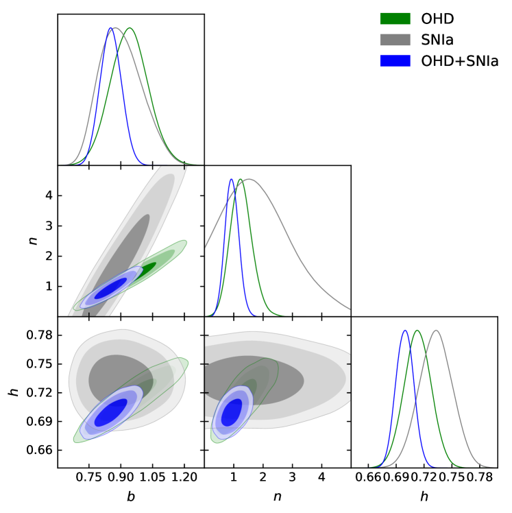
Figure 2: $68$, $97$ and $99.7\%$ CL for free model parameters considering $9\lambda=3\tanh{(bE(z)^{-n})}$.

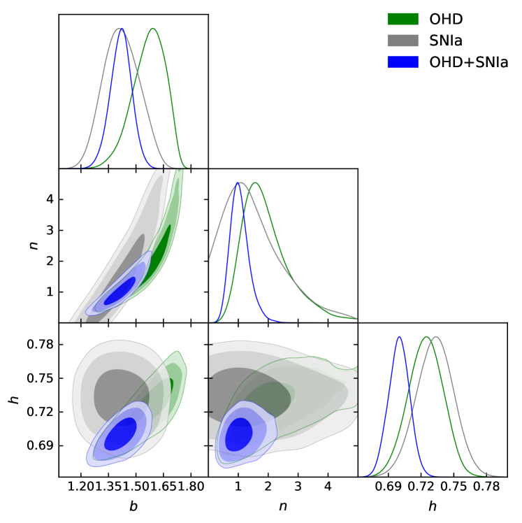
Figure 3: $68$, $97$ and $99.7\%$ CL for the free model parameters considering $9\lambda=\cosh{(bE(z)^{-n})}$.

Figure 4 displays the best curves of the models over $H(z)$ data. To compare with LCDM model we also performed a MCMC joint analysis to obtain its best fitting parameters. Taking into account $\Omega_{r}=2.469\times 10^{-5}h^{-2}(1+0.2271N_{eff})$ where $N_{eff}=3.04$, Komatsu:2011 the best fitting values are $\Omega_{m0}=0.289^{+0.019}_{-0.018}$ and $h=0.712^{+0.013}_{-0.013}$ with a $\chi^{2}=1043.7$. Also we compare our results with one obtained by Normann:2016 when the bulk viscosity is considered in the form $\xi\propto\sqrt{\rho}$.

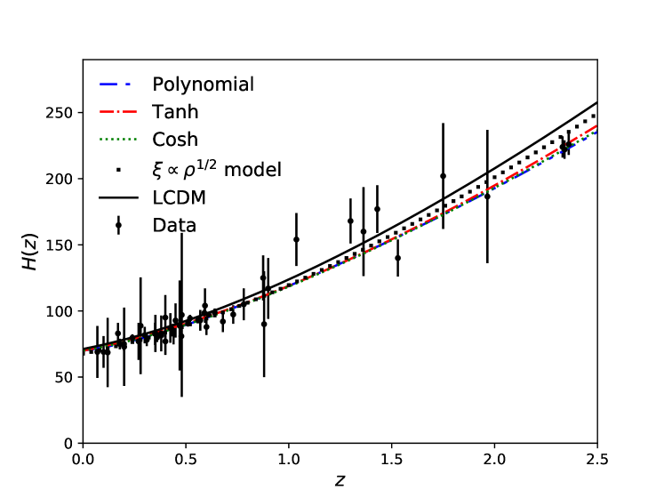
Figure 4: Best fit curves using the results of the joint analysis for LCDM (black solid line), polynomial (blue double dash-dotted line), tanh (red dash-dotted line), and cosh (green dotted line) models. For LCDM, we use $\Omega_{m}=0.289$, and $h=0.712$. The black squares correspond to the bulk viscosity of the form $\xi\propto\rho^{1/2}$ obtained by Normann:2016 . The black points with uncertainty bars correspond to OHD.

Figure 5 shows the reconstruction of the deceleration $q$ (top panel) and jerk $j$ (bottom panel) parameters with respect to the redshift in the region $0<z<2.5$. The Universe filled by the fluids with viscosity present their deceleration-acceleration transition at earlier time ($z_{t}^{pol,tanh,cosh}\approx 0.75$, $0.82$, $0.78$) than the concordance model ($z_{t}^{LCDM}\approx 0.70$). The jerk parameters of the models present the following behavior with respect to LCDM. The jerk parameter for the polynomial model has a lower-bigger transition around $z_{t}^{jerk}\approx 0.50$ and an increasing trend at current epochs. Similarly, the cosh model has a change from lower to bigger values around $z\approx 0.40$ but has a maximum value of less than $1.5$ at current epochs. The tanh model presents jerk values less than 1 for $z<2.5$.

We estimate the $q$ and $j$ parameter values at current epochs $q_{0}=-0.680^{+0.085}_{-0.102}$, $-0.539^{+0.040}_{-0.038}$, $-0.594^{+0.056}_{-0.056}$ and $j_{0}=2.782^{+1.198}_{-0.741}$, $0.297^{+0.051}_{-0.050}$, $1.124^{+0.196}_{-0.178}$ for the polynomial, tanh and cosh models respectively. These $q_{0}$ values are consistent up to $3\sigma$ CL with the one obtained for the LCDM model ($q_{0}^{LCDM}=-0.586^{+0.012}_{-0.011}$). With respect to the current value of the jerk, $j_{0}$, the polynomial (cosh) model presents a deviation within $2.4\sigma$ ($0.7\sigma$) CL with respect to LCDM one ($j^{LCDM}=1$). In contrast, the $j_{0}$ of the tanh model is deviated from the LCDM one of $13.8\sigma$ CL.

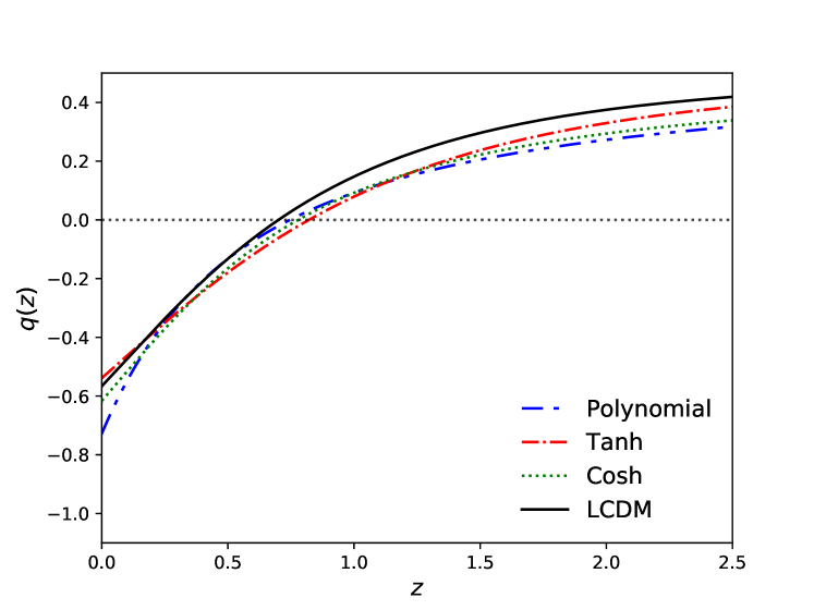
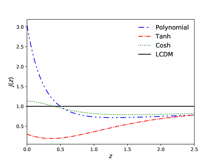
Figure 5: Reconstruction of the deceleration and jerk parameter using the best fit values of the OHD$+$SNIa analysis for LCDM (black solid line), polynomial (blue double dash-dotted line), tanh (red dash-dotted line), and cosh (green dotted line) models.

The Akaike information criterion (AIC) AIC:1974 ; Sugiura:1978 and the Bayesian information criterion (BIC) schwarz1978 are useful tools to compare models statistically defined by ${\rm AIC}=\chi^{2}+2k$ and ${\rm BIC}=\chi^{2}+2k\,\ln(N)$ respectively where $\chi^{2}$ is the chi-square function, $k$ is the number of estimated parameters and $N$ is the number of measurements. In these technique the model preferred by data is the one that has the minimum values on AIC and BIC. Hence taking into account the $\chi^{2}$ yields values reported in Tab. 2 and 3, we obtain ${\rm AIC}^{pol,tanh,cosh}=1063.2$, $1063.7$, $1062.7$ and ${\rm AIC}^{LCDM}=1051.7$, and ${\rm BIC}^{pol,tanh,cosh}=1088.1$, $1083.7$, $1082.7$ and ${\rm BIC}^{LCDM}=1071.6$. Following the convention presented in Liddle:2007 ; Davari:2018 for these criteria, we obtain that the data (OHD + SNIa) prefer a Universe filled with a perfect fluid (LCDM) than one filled by a viscous fluid. Between the phenomenological viscous models, the data prefer equally a Universe filled with a bulk viscosity modeled by a hyperbolic or a polynomial behaviour. Although the polynomial model is a simpler model than the hyperbolic one, it presents a increase behavior at the future as is shown in the statefinder phase-space.

Finally, we analyze the SF diagnostic to distinguish between the behavior of the viscous models from the LCDM model one. In the $\{s,r\}$-SF diagram the LCDM model is a fixed point located at $\{s,r\}=(0,1)$. Figure 6 displays the $\{s,r\}$-SF space of the models in the redshift interval $-1<z<2.5$. The arrows over the trajectories of the models show the evolution direction and the solid squares are the current position ($z=0$) in the $\{s,r\}$-SF plane. We observe that the viscous models have their evolution from the quintessence region to the LCDM model. However, the polynomial model has an increasing behavior in the future with $\{s,r\}$-point $(-3,38.3)$ at $z=-1$ (see the inner plot of Fig. 6), and for the tanh and cosh models end their evolution in the LCDM point.

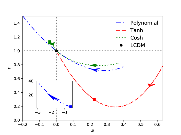
Figure 6: $\{s,r\}$-statefinder diagram using the best fit values of the joint analysis in the redshift region $-1<z<2.5$. The LCDM model is represented by a black solid circle at (0,1). In blue double-dot-dashed line is the trajectory of the polynomial model, and in red dash-dotted (green dotted) line is the trajectory of the tanh (cosh) model. The blue and red (green) solid square markers over the trajectories represent the position at $z=0$. The arrows over the trajectories of the models mean the direction to the future.

5 Conclusions

The present work was devoted to studying the dynamics of the Universe when it is filled by a non-perfect fluid. We analyzed three phenomenological non-perfect fluid models by introducing a bulk viscosity term in the Einstein equations through an effective pressure. The simplest dimensionless bulk viscosity consists of a polynomial function in terms of the redshift introduced by Xin-He:2009 . A more complex model was proposed by FOLOMEEV200875 consisting of a bulk viscosity term of $\tanh$ function. We also studied a phenomenological alternative to the latter by modeling the bulk viscosity as a cosh form. Then we performed a Bayesian MCMC analysis to constrain the free parameters of the viscous models using the latest sample of OHD and SNIa and observe a good agreement of them to the data. When they are seen in the $\{s,r\}$-statefinder space, they behave in the quintessence region. Also, the jerk parameter confirms a dynamical EoS of the viscous models. On the other hand, when we make $n=0$ for the three viscous models, we obtain the simplest case which $\lambda={\rm const}$ or $\xi={\rm const}$. From our best fits, we find a deviation between the constant bulk coefficient and the tanh (cosh) model of about $4.5\sigma$ ($3.7\sigma$) and for the polynomial model, we estimate a limit of $n<-0.54$ at $99\%$ CL. When we compared statistically these models with LCDM, we find that a Universe filled by a non-perfect fluid is equally unsupported by the observational data used over the concordance model.

References

- (1) A.G. Riess, A.V. Filippenko, P. Challis, A. Clocchiatti, A. Diercks, et al., The Astronomical Journal 116(3), 1009 (1998)
- (2) S. Perlmutter, G. Aldering, G. Goldhaber, R.A. Knop, P. Nugent, others, T.S.C. Project, The Astrophysical Journal 517(2), 565 (1999)
- (3) T.M.C. Abbott, et. al, Phys. Rev. D 98, 043526 (2018). DOI 10.1103/PhysRevD.98.043526. URL https://link.aps.org/doi/10.1103/PhysRevD.98.043526
- (4) Planck Collaboration, Ade, P. A. R., et. al., A&A 594, A13 (2016). DOI 10.1051/0004-6361/201525830. URL https://doi.org/10.1051/0004-6361/201525830
- (5) Planck Collaboration, Ade, P. A. R., et. al., A&A 594, A14 (2016). DOI 10.1051/0004-6361/201525814. URL https://doi.org/10.1051/0004-6361/201525814
- (6) S. Alam, et al., Mon. Not. Roy. Astron. Soc. 470, 2617 (2017). DOI 10.1093/mnras/stx721
- (7) M. Persic, P. Salucci, F. Stel, Monthly Notices of the Royal Astronomical Society 281(1), 27 (1996). DOI 10.1093/mnras/278.1.27
- (8) A. Borriello, P. Salucci, Monthly Notices of the Royal Astronomical Society 323(2), 285 (2001). DOI 10.1046/j.1365-8711.2001.04077.x. URL http://dx.doi.org/10.1046/j.1365-8711.2001.04077.x
- (9) C.S. Frenk, A.E. Evrard, S.D.M. White, F.J. Summers, The Astrophysical Journal 472(2), 460 (1996)
- (10) J. Preskill, M.B. Wise, F. Wilczek, Physics Letters B 120(1), 127 (1983). DOI https://doi.org/10.1016/0370-2693(83)90637-8
- (11) L.D. Duffy, K. van Bibber, New Journal of Physics 11(10), 105008 (2009). DOI 10.1088/1367-2630/11/10/105008
- (12) T. Matos, F.S. Guzmán, D. Núñez, Phys. Rev. D 62, 061301 (2000). DOI 10.1103/PhysRevD.62.061301. URL https://link.aps.org/doi/10.1103/PhysRevD.62.061301
- (13) L.A. Ureña López, T. Matos, Phys. Rev. D 62, 081302 (2000). DOI 10.1103/PhysRevD.62.081302. URL https://link.aps.org/doi/10.1103/PhysRevD.62.081302
- (14) T. Matos, F.S. Guzman, Class. Quant. Grav. 18, 5055 (2001). DOI 10.1088/0264-9381/18/23/303
- (15) M. Rodriguez-Meza, Advances in Astronomy 2012, 1 (2012). DOI 10.1155/2012/509682
- (16) M.A. Rodríguez-Meza, AIP Conference Proceedings 1473(1), 74 (2012). DOI http://dx.doi.org/10.1063/1.4748537
- (17) M.A. Rodriguez-Meza, J.L. Cervantes-Cota, Mon. Not. R. Astron. Soc. 350, 671 (2004)
- (18) R. Catena, L. Covi, The European Physical Journal C 74(5), 2703 (2014). DOI 10.1140/epjc/s10052-013-2703-4
- (19) W. Hu, D.J. Eisenstein, Phys. Rev. D 59, 083509 (1999). DOI 10.1103/PhysRevD.59.083509
- (20) M. Kunz, Phys. Rev. D 80, 123001 (2009). DOI 10.1103/PhysRevD.80.123001. URL https://link.aps.org/doi/10.1103/PhysRevD.80.123001
- (21) S. Chaplygin, Sci. Mem. Mosc. Univ. Math. Phys 21(1) (1904)
- (22) A.Yu. Kamenshchik, U. Moschella, V. Pasquier, Phys. Lett. B511, 265 (2001). DOI 10.1016/S0370-2693(01)00571-8
- (23) N. Bilic, G.B. Tupper, R.D. Viollier, Phys. Lett. B535, 17 (2002). DOI 10.1016/S0370-2693(02)01716-1
- (24) J.C. Fabris, S.V.B. Goncalves, P.E. de Souza, Gen. Rel. Grav. 34, 53 (2002). DOI 10.1023/A:1015266421750
- (25) J. Lu, Physics Letters B 680(5), 404 (2009). DOI https://doi.org/10.1016/j.physletb.2009.09.027
- (26) P.H. Chavanis, Physics Letters B 758, 59 (2016). DOI https://doi.org/10.1016/j.physletb.2016.04.042
- (27) H. Hova, H. Yang, International Journal of Modern Physics D 26, 1750178 (2017)
- (28) Hernández-Almada, A., Magaña, Juan, García-Aspeitia, Miguel A., Motta, V., Eur. Phys. J. C 79(1), 12 (2019). DOI 10.1140/epjc/s10052-018-6521-6. URL https://doi.org/10.1140/epjc/s10052-018-6521-6
- (29) W. Zimdahl, Phys. Rev. D 53, 5483 (1996). DOI 10.1103/PhysRevD.53.5483. URL https://link.aps.org/doi/10.1103/PhysRevD.53.5483
- (30) A.A. Coley, R.J. van den Hoogen, R. Maartens, Phys. Rev. D 54, 1393 (1996). DOI 10.1103/PhysRevD.54.1393. URL https://link.aps.org/doi/10.1103/PhysRevD.54.1393
- (31) S. Weinberg, Rev. Mod. Phys. 61, 1 (1989). DOI 10.1103/RevModPhys.61.1. URL https://link.aps.org/doi/10.1103/RevModPhys.61.1
- (32) I. Zlatev, L. Wang, P.J. Steinhardt, Phys. Rev. Lett. 82, 896 (1999). DOI 10.1103/PhysRevLett.82.896. URL https://link.aps.org/doi/10.1103/PhysRevLett.82.896
- (33) I. Brevik, Ø. Grøn, J. de Haro, S.D. Odintsov, E.N. Saridakis, International Journal of Modern Physics D 26(14), 1730024 (2017). DOI 10.1142/S0218271817300245
- (34) R.R. Caldwell, M. Kamionkowski, N.N. Weinberg, Phys. Rev. Lett. 91, 071301 (2003). DOI 10.1103/PhysRevLett.91.071301. URL https://link.aps.org/doi/10.1103/PhysRevLett.91.071301
- (35) I. Brevik, E. Elizalde, S. Nojiri, S.D. Odintsov, Phys. Rev. D 84, 103508 (2011). DOI 10.1103/PhysRevD.84.103508. URL https://link.aps.org/doi/10.1103/PhysRevD.84.103508
- (36) M. Xin-He, R. Jie, H. Ming-Guang, Communications in Theoretical Physics 47(2), 379 (2007). DOI 10.1088/0253-6102/47/2/036
- (37) C. Eckart, Phys. Rev. 58, 919 (1940). DOI 10.1103/PhysRev.58.919. URL https://link.aps.org/doi/10.1103/PhysRev.58.919
- (38) W. Israel, J. Stewart, Annals of Physics 118(2), 341 (1979). DOI https://doi.org/10.1016/0003-4916(79)90130-1
- (39) L.P. Chimento, A.S. Jakubi, V. Méndez, R. Maartens, Classical and Quantum Gravity 14(12), 3363 (1997). DOI 10.1088/0264-9381/14/12/019
- (40) M. Cruz, N. Cruz, S. Lepe, Phys. Rev. D 96, 124020 (2017). DOI 10.1103/PhysRevD.96.124020
- (41) N. Cruz, E. González, S. Lepe, D.S.C. Gómez, Journal of Cosmology and Astroparticle Physics 2018(12), 017 (2018). DOI 10.1088/1475-7516/2018/12/017
- (42) N. Cruz, E. González, G. Palma, arXiv e-prints arXiv:1812.05009 (2018)
- (43) M.M. Disconzi, T.W. Kephart, R.J. Scherrer, Phys. Rev. D 91, 043532 (2015). DOI 10.1103/PhysRevD.91.043532. URL https://link.aps.org/doi/10.1103/PhysRevD.91.043532
- (44) G.L. Murphy, Phys. Rev. D 8, 4231 (1973). DOI 10.1103/PhysRevD.8.4231
- (45) V.A. Belinskii, M. Khalatnikov, Zh. Eksp. Teor. Fiz. 69, 401 (1975)
- (46) I. Brevik, O. Gorbunova, General Relativity and Gravitation 37(12), 2039 (2005). DOI 10.1007/s10714-005-0178-9. URL https://doi.org/10.1007/s10714-005-0178-9
- (47) M. Xin-He, D. Xu, Communications in Theoretical Physics 52(2), 377 (2009). URL http://stacks.iop.org/0253-6102/52/i=2/a=36
- (48) B.D. Normann, I. Brevik, Entropy 18(6) (2016)
- (49) I. Brevik, E. Elizalde, S.D. Odintsov, A.V. Timoshkin, International Journal of Geometric Methods in Modern Physics 14(12), 1750185 (2017). DOI 10.1142/S0219887817501857
- (50) B.D. Normann, I. Brevik, Modern Physics Letters A 32(04), 1750026 (2017). DOI 10.1142/S0217732317500262
- (51) J. Magana, M.H. Amante, M.A. Garcia-Aspeitia, V. Motta, Monthly Notices of the Royal Astronomical Society 476(1), 1036 (2018). DOI 10.1093/mnras/sty260. URL http://dx.doi.org/10.1093/mnras/sty260
- (52) D.M. Scolnic, et. al., The Astrophysical Journal 859(2), 101 (2018). URL http://stacks.iop.org/0004-637X/859/i=2/a=101
- (53) V. Folomeev, V. Gurovich, Physics Letters B 661(2), 75 (2008). DOI https://doi.org/10.1016/j.physletb.2008.01.068
- (54) H. Velten, J. Wang, X. Meng, Phys. Rev. D 88, 123504 (2013). DOI 10.1103/PhysRevD.88.123504
- (55) M.S. Turner, G. Steigman, L.M. Krauss, Phys. Rev. Lett. 52, 2090 (1984). DOI 10.1103/PhysRevLett.52.2090. URL https://link.aps.org/doi/10.1103/PhysRevLett.52.2090
- (56) J.R. Wilson, G.J. Mathews, G.M. Fuller, Phys. Rev. D 75, 043521 (2007). DOI 10.1103/PhysRevD.75.043521. URL https://link.aps.org/doi/10.1103/PhysRevD.75.043521
- (57) G.J. Mathews, N.Q. Lan, C. Kolda, Phys. Rev. D 78, 043525 (2008). DOI 10.1103/PhysRevD.78.043525
- (58) R. Caldwell, Physics Letters B 545(1), 23 (2002). DOI https://doi.org/10.1016/S0370-2693(02)02589-3
- (59) V. Sahni, T.D. Saini, A.A. Starobinsky, U. Alam, Journal of Experimental and Theoretical Physics Letters 77(5), 201 (2003). DOI 10.1134/1.1574831
- (60) U. Alam, V. Sahni, T. Deep Saini, A.A. Starobinsky, Monthly Notices of the Royal Astronomical Society 344(4), 1057 (2003). DOI 10.1046/j.1365-8711.2003.06871.x. URL http://dx.doi.org/10.1046/j.1365-8711.2003.06871.x
- (61) A. Al Mamon, K. Bamba, The European Physical Journal C 78(10), 862 (2018). DOI 10.1140/epjc/s10052-018-6355-2. URL https://doi.org/10.1140/epjc/s10052-018-6355-2
- (62) D. Foreman-Mackey, D.W. Hogg, D. Lang, J. Goodman, pasp 125, 306 (2013). DOI 10.1086/670067
- (63) A. Gelman, D. Rubin, Statistical Science 67, 457 (1992). DOI 10.1103/PhysRevD.67.101301. URL https://link.aps.org/doi/10.1103/PhysRevD.67.101301
- (64) R. Jimenez, A. Loeb, Astrophys. J. 573, 37 (2002). DOI 10.1086/340549
- (65) E. Komatsu, et al., Astrophys. J. Suppl. 192, 18 (2011). DOI 10.1088/0067-0049/192/2/18
- (66) H. Akaike, IEEE Transactions on Automatic Control 19(6), 716 (1974). DOI 10.1109/TAC.1974.1100705
- (67) N. Sugiura, Communications in Statistics - Theory and Methods 7(1), 13 (1978). DOI 10.1080/03610927808827599. URL https://doi.org/10.1080/03610927808827599
- (68) G. Schwarz, Ann. Statist. 6(2), 461 (1978). DOI 10.1214/aos/1176344136. URL https://doi.org/10.1214/aos/1176344136
- (69) A.R. Liddle, Monthly Notices of the Royal Astronomical Society: Letters 377(1), L74 (2007). DOI 10.1111/j.1745-3933.2007.00306.x. URL https://dx.doi.org/10.1111/j.1745-3933.2007.00306.x
- (70) Z. Davari, M. Malekjani, M. Artymowski, Phys. Rev. D 97, 123525 (2018). DOI 10.1103/PhysRevD.97.123525