Barium and related stars, and their white-dwarf companions ^,

Abstract

Context. Barium and S stars without technetium are red giants suspected of being all members of binary systems.

Aims. This paper provides both long-term and revised, more accurate orbits for barium and S stars adding to previously published ones. The sample of barium stars with strong anomalies comprise all such stars present in the Lü et al. catalogue.

Methods. Orbital elements are derived from radial velocities collected from a long-term radial-velocity monitoring performed with the HERMES spectrograph mounted on the Mercator 1.2 m telescope. These new measurements were combined with older, CORAVEL measurements. With the aim of investigating possible correlations between orbital properties and abundances, we collected as well an as homogeneous as possible set of abundances for barium stars with orbital elements.

Results. We find orbital motion for all barium and extrinsic S stars monitored. We obtain the longest period known so far for a spectroscopic binary involving an S star, namely 57 Peg with a period of the order of 100 – 500 yr. We present the mass distribution for the barium stars, which ranges from 1 to 3 M_⊙, with a tail extending up to 5 M_⊙ in the case of mild barium stars. This high-mass tail comprises mostly high-metallicity objects ([Fe/H] $\geq-0.1$). Mass functions are compatible with WD companions whose masses range from 0.5 to 1 M_⊙. Strong barium stars have a tendency to be found in systems with shorter periods than mild barium stars, although this correlation is rather lose, metallicity and WD mass playing a role as well. Using the initial – final mass relationship established for field WDs, we derived the distribution of the mass ratio $q^{\prime}=M_{\rm AGB,ini}/M_{\rm Ba}$ (where $M_{\rm AGB,ini}$ is the WD progenitor initial mass, i.e., the mass of the system former primary component) which is a proxy for the initial mass ratio (the more so, the less mass the barium star has accreted). It appears that the distribution of $q^{\prime}$ is highly non uniform, and significantly different for mild and strong barium stars, the latter being characterized by values mostly in excess of 1.4, whereas mild barium stars occupy the range 1 – 1.4.

Conclusions. The orbital properties presented in this paper pave the way for a comparison with binary-evolution models.

1 Introduction

Barium stars (Bidelman & Keenan, 1951) are a class of G-K red-giant stars with strong spectral lines of barium and other elements produced by the slow neutron-capture process (s-process; e.g., Käppeler et al., 2011). Similar spectral peculiarities are also found in main sequence stars known as barium dwarfs, which cover spectral types all the way from F to K (North et al., 1994). Another related family comprises S stars (Keenan, 1954), which are giants cooler than barium stars, exhibiting ZrO bands in their spectra. As shown by Smith & Lambert (1988) and Jorissen et al. (1993) for example, two kinds of S stars arise: Tc-rich (also known as intrinsic) and no-Tc (also known as extrinsic) S stars, depending on the presence or absence of Tc lines, an element with no stable isotopes. Extrinsic S stars are the cooler analogs of barium stars.

These families of stars exhibiting strong lines of s-process elements have been intensively studied in the past (e.g., Burbidge & Burbidge, 1957; Warner, 1965; McClure et al., 1980; Boffin & Jorissen, 1988; McClure & Woodsworth, 1990; Jorissen & Mayor, 1992; North et al., 1994; Jorissen et al., 1998; North et al., 2000; de Castro et al., 2016; Merle et al., 2016), being benchmarks of post mass-transfer binaries involving low- and intermediate-mass stars. They provide strong constraints on the mass-transfer phase they experienced when the former primary, now a white dwarf, was an asymptotic giant branch (AGB) star and transferred material enriched in heavy elements produced by the s-process of nucleosynthesis (e.g., Käppeler et al., 2011), among which is barium. The polluted companion indeed kept this chemical signature up to now, long after the mass transfer ceased, and exhibits strong absorption lines of ionised barium in its spectrum. This binary scenario was convincingly confirmed by the observation that statistically all barium stars reside in binary systems (McClure et al., 1980; McClure, 1983; Jorissen & Mayor, 1988; McClure & Woodsworth, 1990; Jorissen et al., 1998).

Previous binary-evolution models have shown how difficult it is to account for the orbital properties of these objects (Pols et al., 2003; Jorissen, 2003; Bonačić Marinović et al., 2008). These models need improved prescriptions for the mass-transfer process (Frankowski & Jorissen, 2007; Izzard et al., 2010; Dermine et al., 2011). These studies have shown how important it is to derive the orbital periods and eccentricities of post-mass-transfer systems such as barium stars in order to constrain evolutionary models. CH and carbon-enriched metal-poor (CEMP) stars are post-mass-transfer objects as well, albeit of low metallicity, and new and updated orbits for these classes were presented in a recent paper (Jorissen et al., 2016). Post-AGB stars with a near-infrared excess indicative of a dusty disk form another possibly related family of post-mass-transfer objects (e.g., Van Winckel et al., 2009; Oomen et al., 2018).

Orbital elements provide constraints on evolutionary models through the period–eccentricity ($P-e$) diagram and the mass-function distribution, which is sensitive to the mass of the companion. For post-mass-transfer systems (like barium, CH, and CEMP-s systems enriched in heavy elements synthesised by the s-process), the companion should be a CO white dwarf (Merle et al., 2016). This paper presents the orbits for all known giant barium stars with strong chemical anomalies (i.e., all those classified as Ba3, Ba4, or Ba5 in the 1983 edition of the Lü et al. catalog), plus an extended sample of mild barium stars, along with their cooler analogs, the extrinsic S stars lacking the unstable element technetium. A detailed analysis of the mass functions, the mass-ratio and mass distributions, the $P-e$ diagram, and their relationship with chemical pollution concludes this paper. A twin paper (Escorza et al., 2019) addresses the same questions for dwarf barium stars.

2 Samples of barium and S stars without Tc

The present study is a follow-up of the monitoring campaign of barium and S stars initiated in 1984 with the CORAVEL spectrograph (Baranne et al., 1979), the results of which were presented in Jorissen & Mayor (1988, 1992), Jorissen et al. (1998), and Udry et al. (1998a, b).

The CORAVEL monitoring was not able to derive all the orbits either because several turned out to be much longer than its time span, or because its precision (about 0.3 km s^-1) was not good enough to detect the orbits with the smallest semi-amplitudes (like 0.6 km s^-1  for HD 183915 and HD 189581, as we report in Sect. 4.3). These shortcomings motivated the pursuit of this former monitoring campaign after several years of interruption, with a much more accurate spectrograph (HERMES, as described in Sect. 3) than the old CORAVEL. The new monitoring, described in e.g., Van Winckel et al. (2010) and Gorlova et al. (2013), could therefore reveal binary systems with much lower velocity amplitudes, not accessible to CORAVEL.

The sample comprises all 37 barium stars with strong chemical anomalies (dubbed Ba3, Ba4, or Ba5 in Warner scale; Warner, 1965) from the list of Lü et al. (1983), as well as 40 among the mild barium stars of that list. Although the latter sample is by no means complete, it provides a good comparison to the (complete) sample of strong barium stars. The binary status of the targets mentioned in the list below refers to the situation prevailing at the start of the HERMES monitoring.

The sample of barium stars monitored by HERMES is comprised of the following.

• 2 strong barium stars (HD 123949, HD 211954) with long and uncertain orbital periods;

• 1 strong barium star with no evidence for binary motion (HD 65854);

• 11 mild barium stars with long, uncertain periods (HD 22589, HD 53199, HD 196673), or with a lower limit on the period (HD 40430, HD 51959, HD 98839, HD 101079, HD 104979, HD 134698, HD 165141, BD $-10^{\circ}$4311);

• 3 suspected binaries (HD 18182, HD 183915, HD 218356) among mild barium stars, and 3 mild barium stars with no evidence for binary motion (HD 50843, HD 95345, HD 119185).

The S-star sample monitored by HERMES is constructed as follows.

• 6 stars (HD 30959 = $o^{1}$ Ori, HD 184185, HD 218634, HDE 288833, BD+31^∘4391, and BD+79^∘156) with a lower limit on the orbital period from Table 3a of Jorissen et al. (1998);

• 2 stars with no Tc lines and no evidence for binarity (BD $-21^{\circ}$2601 and HD 189581) from Table 3c of Jorissen et al. (1998);

• 4 poorly studied symbiotic S stars not present in the original sample of Jorissen et al. (1998): Hen 4-18, V420 Hya, and ER Del from Van Eck & Jorissen (2002) and HR 363 from Jorissen et al. (1996).

To these twelve S stars monitored by HERMES, 22 supplementary systems with orbital elements already obtained by CORAVEL (as listed in Table 3a of Jorissen et al., 1998) must be added. In total, the sample of S stars monitored thus comprises 34 objects.

3 Radial-velocity monitoring with the HERMES spectrograph

The radial-velocity (RV) monitoring was performed with the HERMES spectrograph attached to the 1.2m Mercator telescope from the Katholieke Universiteit Leuven, installed at the Roque de los Muchachos Observatory (La Palma, Spain). The spectrograph began regular science observations in April 2009, and is fully described in Raskin et al. (2011). The fiber-fed HERMES spectrograph is designed to be optimized both in stability as well as in efficiency. It samples the whole optical range from 380 to 900 nm in one shot, with a spectral resolution of about $86\,000$ for the high-resolution science fiber. This fiber has a 2.5 arcsec aperture on the sky and the high resolution is reached by mimicking a narrow slit using a two-sliced image slicer.

The MERCATOR-HERMES combination is precious because it guarantees regular telescope time. This is needed for our monitoring programme and the operational agreement reached by all consortium partners (KULeuven, Université libre de Bruxelles, Royal Observatory of Belgium, Landessternwarnte Tautenburg) is optimized to allow efficient long-term monitoring, which is indispensable for this programme. The long-term monitoring of barium and S stars is performed within the framework of this HERMES consortium, with some further data points acquired during KULeuven observing runs (Van Winckel et al., 2010; Gorlova et al., 2013). In total, about 200 nights per year are devoted to this monitoring campaign, and the observation sampling is adapted to the known variation timescale.

A Python-based pipeline extracts a wavelength-calibrated, cosmic-ray cleaned spectrum. A separate routine is used for measuring RVs, by means of a cross-correlation with a spectral mask constructed on an Arcturus spectrum. A restricted region covering the range 478.11 – 653.56 nm (orders 55 – 74) and containing 1543 useful spectral lines was used to derive the RV, in order to avoid telluric lines on the red end, and often poorly exposed and crowded spectrum on the blue end. A spectrum with a signal-to-noise ratio of 20 is usually sufficient to obtain a cross-correlation function (CCF) with a well-defined minimum. An example of CCF is shown in Fig. 1 of Jorissen et al. (2016).

A Gaussian fit is performed on the CCF, and delivers an internal precision of less than 10 m s^-1 on the position of the center (depending on the CCF shape). The absolute precision of a single RV measurement is $\sim 200$ m/s, limited by the pressure fluctuations during the night in the spectrograph room (see Fig. 9 of Raskin et al., 2011). However, this drift has no effect if the arc spectrum used for wavelength calibration is taken consecutive to the science exposure. The long-term accuracy (i.e., over several years) may be estimated from the stability of the RV standard stars monitored along with the science targets. These standard stars are taken from the list of Udry et al. (1999), available at http://obswww.unige.ch/$\sim$udry/std/std.html. The distribution of the standard-star velocity standard deviations peaks at $\sigma(Vr)=55$ m s^-1 (as shown in Fig. 2 of Jorissen et al., 2016), which may thus be adopted as the typical uncertainty on the radial velocities over the long term.

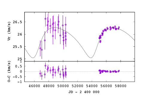
Figure 22: Upper panel: Radial velocities of the mild barium star HD 18182 and a preliminary orbit with $P=22$ yr and $e=0.3$. Older data are from CORAVEL, newer from HERMES. A zero point offset of +0.6 km s^-1  has been applied to the CORAVEL measurements. Lower panel: O-C residuals.

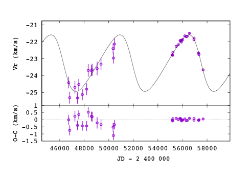
Figure 23: Upper panel: Radial velocities of the mild barium star HD 40430 and a preliminary orbit with $P=15$ yr and $e=0.22$. Older data are from CORAVEL, newer from HERMES. Lower panel: O-C residuals.

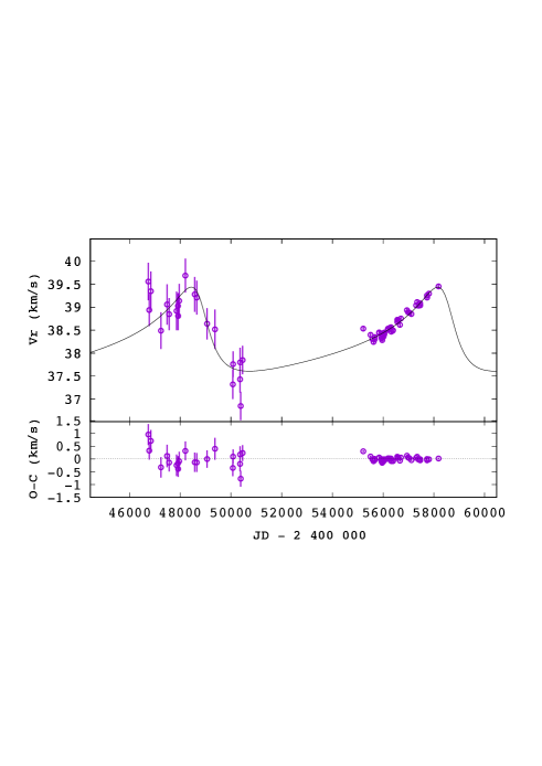
Figure 24: Upper panel: Radial velocities of the mild barium star HD 51959 and a preliminary orbit with $P=27$ yr and $e=0.53$. Older data are from CORAVEL, newer from HERMES. Lower panel: O-C residuals.

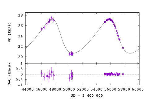
Figure 25: Upper panel: Radial velocities of the mild barium star HD 53199 and the associated orbit. Older data are from CORAVEL, newer from HERMES. An offset of +0.4 km s^-1  has been applied to the CORAVEL data. Lower panel: O-C residuals.

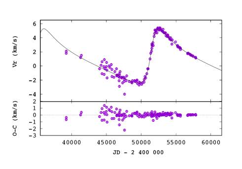
Figure 26: Upper panel: Radial velocities of the mild barium star HD 98839 (= 56 UMa) and the associated orbit. Older data are from Griffin (2008a), newer are from HERMES, according to Table 3. In this figure, the HERMES velocities are offset by +0.6 km s^-1  to ensure consistency with Griffin’s velocities. Lower panel: O-C residuals.

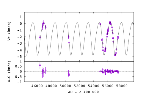
Figure 27: Upper panel: Radial velocities of the mild barium star HD 101079 and the associated orbit. Older data are from CORAVEL, newer from HERMES. An offset of +0.5 km s^-1  has been applied to the CORAVEL data. Lower panel: O-C residuals.

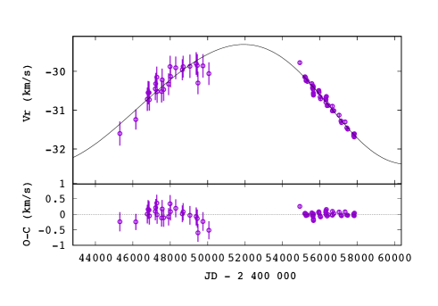
Figure 28: Same as Fig. 22 but for a preliminary orbit of HD 104979 with $P=53$ yr and $e=0.1$. An offset of +0.5 km s^-1  has been applied to the CORAVEL data.

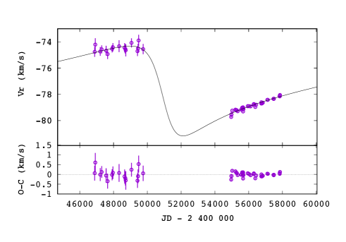
Figure 29: Upper panel: Radial velocities of the mild barium star HD 119185 and a preliminary orbit with $P=60$ yr and $e=0.6$! Older data are from CORAVEL, newer from HERMES. Lower panel: O-C residuals.

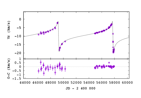
Figure 30: Upper panel: Radial velocities of the strong barium star HD 123949 and the associated orbit, having $P=23.3$ yr and $e=92$. Older data are from CORAVEL, newer from HERMES. An offset of +0.7 km s^-1  has been applied to the CORAVEL data. Lower panel: O-C residuals.

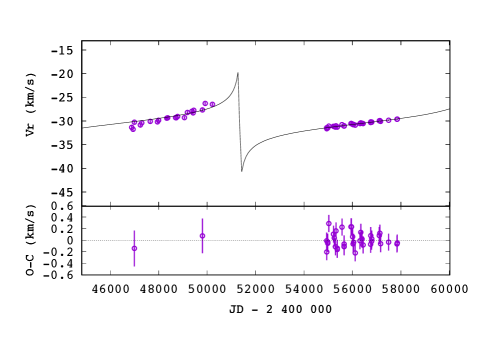
Figure 31: Upper panel: Radial velocities of the mild barium star HD 134698 and a preliminary orbit with $P=27$ yr and $e=0.95$. Older data are from CORAVEL, newer from HERMES. An offset of +0.5 km s^-1  has been applied to the CORAVEL data. Lower panel: O-C residuals, only shown for the data points used in the orbit derivation (see Sect. 5.4). The other CORAVEL data are displayed as blue crosses in the upper panel.

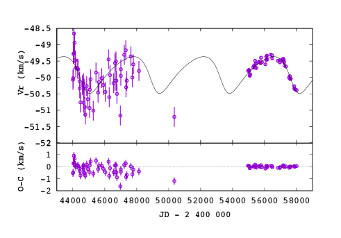
Figure 32: Upper panel: Radial velocities of the mild barium star HD 183915 and the associated orbit. Older data are from CORAVEL, newer from HERMES. Lower panel: O-C residuals.

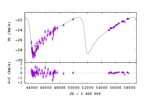
Figure 33: Upper panel: Radial velocities of the mild barium star HD 196673 and the associated orbit. Older data are from CORAVEL, newer from HERMES. Lower panel: O-C residuals.

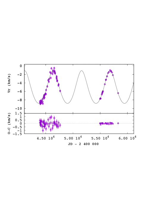
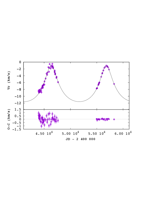
Figure 34: Two possible orbital solutions for the mild barium star HD 199394. Top panel: Preliminary solution with $P=14.3$ yr and $e=0.11$; Bottom panel: Another solution with $P=$28.7 y, and $e=$0.36 is also possible, although less likely given its associated mass function of $0.128\pm 0.007$ M_⊙, as compared to $0.030\pm 0.001$ M_⊙ for the 14 yr orbit. Older data are from CORAVEL, newer from HERMES. Lower panels: O-C residuals. An offset of +0.5 km s^-1 has been applied to the CORAVEL data.

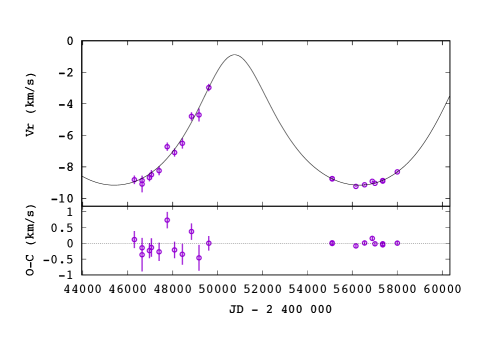
Figure 35: Upper panel: Radial velocities of the strong barium star HD 211954 and the associated orbit. Older data are from CORAVEL, newer from HERMES. Lower panel: O-C residuals.

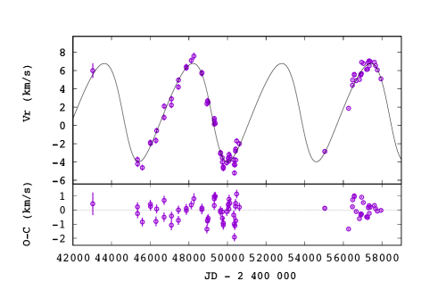
Figure 36: Upper panel: Radial velocities of the symbiotic S star HD 7351 = HR 363 and the associated orbit. Older data are from CORAVEL, newer from HERMES. Lower panel: O-C residuals.

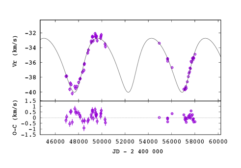
Figure 37: Upper panel: Radial velocities of the S star HD 170970 and the associated orbit. Older data are from CORAVEL, newer from HERMES. Lower panel: O-C residuals.

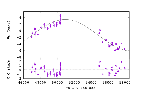
Figure 38: Upper panel: Radial velocities of the S star HD 184185 and a preliminary orbit with $P=43$ yr and $e=0$. Older data are from CORAVEL, newer from HERMES. Lower panel: O-C residuals.

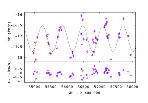
Figure 39: Upper panel: Radial velocities of the S star HD 189581 and the associated orbit. Lower panel: O-C residuals.

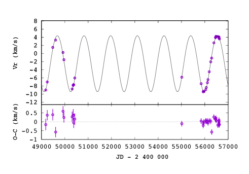
Figure 40: Upper panel: Radial velocities of the S star HD 215336 and the associated orbit. Older data are from CORAVEL, newer from HERMES. Lower panel: O-C residuals.

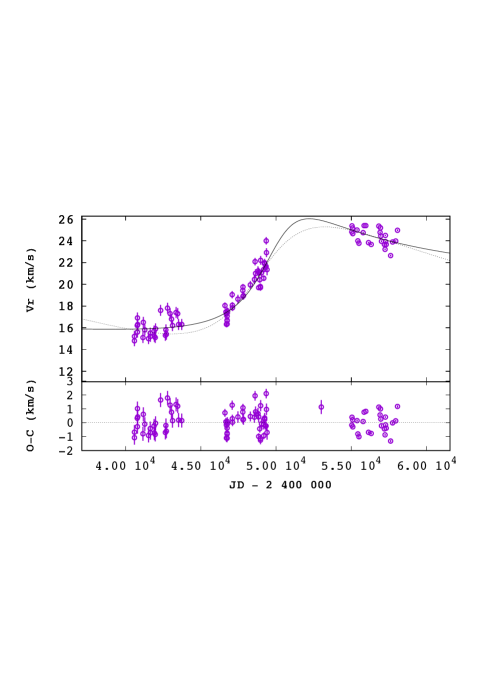
Figure 41: Upper panel: Radial velocities of the S star HD 218634 (57 Peg) and preliminary orbits with $P=532$ yr and $e=0.8$ (solid line), or $P=106$ yr and $e=0.4$ (dashed line). Older CORAVEL data are from R. Griffin (priv. comm.), newer from HERMES. Lower panel: O-C residuals.

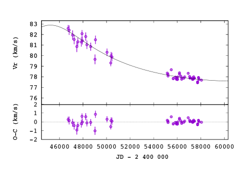
Figure 42: Upper panel: Radial velocities of the S star HDE 288833 and a preliminary orbit with $P=78$ yr and $e=0.35$! Older data are from CORAVEL, newer from HERMES. Lower panel: O-C residuals.

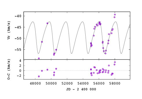
Figure 48: Upper panel: Radial velocities of the S star ER Del and the associated orbit. Older data are from CORAVEL, newer from HERMES. Lower panel: O-C residuals.

The difference between the standard-star-catalogue velocity and the measured value is on average 4 m s^-1 with a standard deviation of 109 m s^-1. This difference of 4 m s^-1 indicates that there is no zero-point offset between HERMES and Udry et al. (1999) list of standard velocity stars. The standard radial-velocity stars from Udry et al. (1999) are tied to the ELODIE velocity system (see Udry et al. 1999 for more details), but the CORAVEL radial velocities used here are on the old CORAVEL system, before its conversion to the ELODIE system. Hence, a zero-point offset needs to be applied to these old measurements in order to make them compatible with the ELODIE/HERMES system. However, this zero-point offset is not easy to predict accurately because it depends on stellar velocity and color. Consequently, its value was, whenever possible, derived a posteriori by ensuring minimal orbital residuals $O-C$ (as displayed by the bottom panels of Figs. 21 and 22–48). The applied offset is given in the caption of these figures displaying the orbital solutions.

4 Results of radial-velocity monitoring

4.1 Binary frequency

This section reviews the binary frequency for barium and (extrinsic) S stars. It updates our previous review (Jorissen et al., 1998) with the new results from the HERMES monitoring. Our 1998 review concluded that 35 out of 37 barium stars with strong chemical anomalies, 34 out of 40 mild barium stars (plus an additional 3 stars with binary suspicion), and 25 out of 27 Tc-poor S stars showed evidence of being binary systems.

The present situation is summarized in Table 1, which also includes stars monitored by McClure at the Dominion Astrophysical Observatory (McClure et al., 1980; McClure, 1983; McClure & Woodsworth, 1990).

For S stars, the two stars (HD 189581 and BD $-21^{\circ}$2601) previously lacking evidence for orbital motion now reveal their binary nature, thanks to the more accurate HERMES data (see Fig. 18 for BD $-21^{\circ}$2601 and Fig. 39 for HD 189581).

Table 1: Updated binary frequency among barium and S star samples from Jorissen et al. (1998). The S stars with radial-velocity jitter were not included. SB19 and SB98 stand for the number of spectroscopic binaries known in 2019 (present paper) and in 1998 (before HERMES), respectively, SBO denotes spectroscopic binaries with either good or preliminary orbits, SB stands for spectroscopic binaries with no orbit available yet, and SB? stands for suspected spectroscopic binary.

Class	$N$	SB19	SB98	SBO			SB	SB?	no evidence SB	New HERMES SBO
				total	good	preliminary
Strong barium (Ba 3,4,5)	37	37	35	36	36	0	1a	0	0	2
Mild barium (Ba 1,2)	40	40	34	37	32	5	2b	1c	0	15
S (no Tc)	34	34	25/27	32	29	3	2d	0	0	14

Notes: (a) HD 19014 (b) HD 50843, HD 65854 (c) HD 95345 (d) BD $-21^{\circ}$2601, T Sgr

All barium stars monitored with HERMES (but one, HD 95345, as discussed below) now show clear signatures of binarity, although orbits are not yet available for all of them. For instance, HD 50843 and HD 65854 are clearly long-period binaries of small amplitude (Figs. 19 and 20), irrespective of the uncertain zero-point offset, since the HERMES data alone reveal a clear drift. There is not enough data yet to look for an orbital solution however.

The situation is not as clear for HD 95345, since there is a short-period, very low-amplitude ($K=78\pm 11$ m s^-1, thus not significantly above the instrumental error; see Sect. 3) orbit possibly fitting the HERMES data points (bottom panel of Fig. 21 and Table 4). Since the standard dispersion of the $O-C$ residuals amounts to 73 m s^-1, almost identical to the semi-amplitude $K$ of the orbit, the significance of this orbit should be considered as very low. In the absence of any long-term drift, an offset of 0.6 km s^-1  is needed to bring the old CORAVEL measurements in agreement with the new HERMES ones (this offset has been applied in the upper panel of Fig. 21). Since this zero-point offset is of the same order as that applied to other barium stars, there is therefore no indication in favor of the duplicity of this star, which could nevertheless be a binary system seen very close to face-on.

HD 19014 is a star monitored by the southern CORAVEL (Udry et al., 1998a) but not by HERMES (because it is located too far south). Evidence for binarity is nevertheless provided by the comparison of the old CORAVEL velocities, yielding an average velocity of $13.3\pm 0.11$ km s^-1  (Table 2b of Jorissen et al., 1998), with the Gaia DR2 velocity of $15.98\pm 0.17$ km s^-1  (Gaia Collaboration et al., 2018). There is thus a difference of 2.7 km s^-1  between the two data sets. To assess whether this difference is a signature of duplicity or is caused by an offset between CORAVEL and Gaia DR2, we compared the average velocities obtained in these two monitoring campaigns for the supposedly constant star HD 95345 described above. Gaia DR2 yields $6.2\pm 0.2$ km s^-1, in perfect agreement with the HERMES and CORAVEL results (after applying the +0.6 km s^-1  offset to the latter; see top panel of Fig. 21). This comparison confirms that the CORAVEL/Gaia-DR2 offset is not expected to be larger than a few tenths of a kilometer per second. Consequently, the difference of 2.7 km s^-1  obtained between the measurements of CORAVEL and Gaia DR2 is very unlikely to be of instrumental origin, and probably indicates that HD 19014 belongs to a binary system.

It is interesting to extend this comparison to the stars HD 50843 and HD 65854, for which HERMES data reveal a low-amplitude long-term drift. For them, Gaia DR2 yields $13.95\pm 0.15$ and $0.82\pm 0.17$ km s^-1, respectively, as compared to the HERMES values of $\sim 13.7$ and $\sim 0.8$ km s^-1  (Figs. 19 and 20). Also in these two stars, HERMES and Gaia DR2 agree within a few tenths of a kilometer per second, despite the long-term drifts.

4.2 Individual radial velocities

The individual radial velocities, referring to the barycenter of the solar system (from IRAF astutils routine using the Stumpff 1980 ephemeris), are presented in Table 2 (for barium stars) and Table 3 (for S stars). The CORAVEL radial velocities (described in the papers by Udry et al., 1998a, b) used to compute the orbital solutions are repeated here.

The data before JD $2\,455\,000$ are from the CORAVEL monitoring (Jorissen & Mayor, 1988; Jorissen et al., 1998), and the more recent data are from HERMES (Van Winckel et al., 2010; Gorlova et al., 2013). No zero-point correction has been applied to the data listed in Tables 2 and 3, although the recommended value is listed in column 6.

As discussed in Sect. 3, the HERMES radial velocities are tied to the ELODIE system, defined by the RV standard stars of Udry et al. (1999), while the CORAVEL data are still on the old (pre-1999) CORAVEL system.

Table 2: Individual radial velocities for barium stars with no offset applied. The recommended offset is listed in the last column. The full table is only available as online material.

Star	JD	$Vr$	$\epsilon(Vr)$	Instrument	Offset
		(km s-1)	(km s-1)		(km s-1)
HD 18182	2446819.2676	24.830	0.320	CORAVEL	0.6
HD 18182	2447036.6647	24.770	0.370	CORAVEL	0.6
HD 18182	2447455.5471	25.150	0.370	CORAVEL	0.6
HD 18182	2447540.3287	26.030	0.310	CORAVEL	0.6
HD 18182	2447838.4685	25.770	0.320	CORAVEL	0.6
HD 18182	2447911.2653	25.920	0.320	CORAVEL	0.6
HD 18182	2448229.4530	25.740	0.300	CORAVEL	0.6
HD 18182	2448569.5505	25.810	0.330	CORAVEL	0.6
HD 18182	2448586.3953	25.330	0.340	CORAVEL	0.6
HD 18182	2448648.2547	25.850	0.310	CORAVEL	0.6
HD 18182	2448917.5595	25.660	0.360	CORAVEL	0.6
HD 18182	2449308.4279	25.790	0.340	CORAVEL	0.6
HD 18182	2449374.2786	25.910	0.300	CORAVEL	0.6
HD 18182	2449606.6341	25.350	0.350	CORAVEL	0.6
HD 18182	2449955.6304	25.760	0.410	CORAVEL	0.6
HD 18182	2450039.4590	25.270	0.310	CORAVEL	0.6
HD 18182	2450071.3952	25.150	0.360	CORAVEL	0.6
HD 18182	2450342.5884	25.330	0.330	CORAVEL	0.6
HD 18182	2450353.6565	25.450	0.380	CORAVEL	0.6
HD 18182	2450354.5067	24.790	0.320	CORAVEL	0.6
HD 18182	2450379.5194	25.190	0.300	CORAVEL	0.6
HD 18182	2455037.7017	25.845	0.045	HERMES	0.0
HD 18182	2455085.7070	25.850	0.044	HERMES	0.0
HD 18182	2455085.7231	25.852	0.044	HERMES	0.0
HD 18182	2455106.6543	25.919	0.043	HERMES	0.0
HD 18182	2455160.4400	25.688	0.043	HERMES	0.0
…

Table 3: As in Table 2 but for S stars. The full table is only available as online material.

Star	JD	$Vr$	$\epsilon(Vr)$	Instrument	Offset
		(km s-1)	(km s-1)		(km s-1)
CD-28 3719	2448643.6500	72.180	0.620	CORAVEL	0.0
CD-28 3719	2449056.5220	71.310	0.430	CORAVEL	0.0
CD-28 3719	2449404.6210	72.680	0.470	CORAVEL	0.0
CD-28 3719	2449801.5420	73.450	0.430	CORAVEL	0.0
CD-28 3719	2450468.7230	59.660	0.410	CORAVEL	0.0
CD-28 3719	2450471.6830	60.760	0.420	CORAVEL	0.0
CD-28 3719	2455222.5241	57.738	0.070	HERMES	0.0
CD-28 3719	2455619.4348	57.979	0.070	HERMES	0.0
CD-28 3719	2455660.3596	62.429	0.067	HERMES	0.0
CD-28 3719	2455859.7530	68.442	0.069	HERMES	0.0
CD-28 3719	2455932.5593	59.682	0.074	HERMES	0.0
CD-28 3719	2455935.5595	59.184	0.070	HERMES	0.0
CD-28 3719	2455958.4853	58.000	0.073	HERMES	0.0
CD-28 3719	2455992.3629	56.971	0.064	HERMES	0.0
CD-28 3719	2456015.3915	58.447	0.079	HERMES	0.0
CD-28 3719	2456316.4978	61.129	0.064	HERMES	0.0
CD-28 3719	2456317.5105	60.907	0.071	HERMES	0.0
CD-28 3719	2456321.4947	59.900	0.074	HERMES	0.0
CD-28 3719	2456349.4299	57.758	0.062	HERMES	0.0
CD-28 3719	2456563.7395	71.906	0.080	HERMES	0.0
CD-28 3719	2456598.7162	72.522	0.077	HERMES	0.0
CD-28 3719	2456608.7550	72.060	0.069	HERMES	0.0
CD-28 3719	2456662.5537	67.903	0.086	HERMES	0.0
CD-28 3719	2456668.5507	67.078	0.079	HERMES	0.0
CD-28 3719	2456700.4912	63.563	0.059	HERMES	0.0
CD-28 3719	2457461.3750	66.854	0.072	HERMES	0.0
…

4.3 Orbits

The orbital elements of the newly derived orbits are listed in Table 4. Some among these are not yet well constrained. For barium stars, these are HD 18182, HD 104979, HD 119185, HD 134698, and HD 199394. Among S stars, HD 184185, HD 218634 (57 Peg), and HDE 288833 have poorly constrained orbital elements. All figures with the orbital solution superimposed on the radial-velocity data are presented in Appendix B. The orbital elements derived earlier may be found in Jorissen et al. (1998) and Udry et al. (1998a, b).

Before proceeding to the analysis of this orbital material in Sects. 6 and 7, we hereafter comment on individual stars.

Table 4: New, revised, and preliminary orbital elements (the latter data are followed by ”:”).

HD/DM	Period	$e$	$V_{\gamma}$	$T_{0}$	$K$	$\omega$	$a_{1}\mathrm{sin}\;i$	$f(m)$	$\sigma$(O-C)	$N$
	(d)		(km s-1)		(km s-1)	(∘)	(Gm)	(M⊙)	(km s-1)
Mild Ba stars
18182	8059:	0.3:
40430	$5609\pm 55$	$0.22\pm 0.01$	$-23.27\pm 0.04$	$2463116\pm 80$	$1.67\pm 0.06$	$88\pm 5$	$126\pm 7$	$0.0025\pm 0.0004$	0.31	36
51959	$9718\pm 157$	$0.53\pm 0.04$	$38.21\pm 0.04$	$2458537\pm 113$	$0.92\pm 0.06$	$50\pm 5$	$104\pm 11$	$0.00047\pm 0.00014$	0.23	64
53199	$8314\pm 99$	$0.24\pm 0.01$	$23.6\pm 0.1$	$2448483\pm 117$	$3.3\pm 0.1$	$63\pm 3$	$364\pm 14$	$0.028\pm 0.003$	$0.09$	$51$
95345	485?	0.3?			$0.08\pm 0.01$?
98839b	$16471\pm 113$	$0.560\pm 0.005$	$0.13\pm 0.01$	$2451547\pm 17$	$3.86\pm 0.03$	$288.9\pm 0.7$	$724\pm 13$	$0.056\pm 0.002$	0.41	143
101079	$1565.8\pm 1.7$	$0.175\pm 0.005$	$-2.000\pm 0.007$	$2458486\pm 6$	$2.48\pm 0.02$	$139.9\pm 1.2$	$52.6\pm 0.4$	$0.00236\pm 0.00005$	0.13	$55$
104979	19295:	0.1:
119185	22065:	0.6:
134698	10005:	0.95:
183915	$4382\pm 21$	$0.27\pm 0.02$	$-49.83\pm 0.01$	$2462214\pm 80$	$0.56\pm 0.01$	$130\pm 6$	$32.6\pm 0.8$	$(7.2\pm 0.5)^{-5}$	0.36	98
196673	$7780\pm 117$	$0.59\pm 0.02$	$-24.2\pm 0.1$	$2451698\pm 128$	$3.7\pm 0.1$	$116\pm 2$	$314\pm 20$	$0.020\pm 0.003$	0.40	$75$
199394	5232:d	0.11:
Strong Ba stars
123949	$8523\pm 8$	$0.9162\pm 0.0003$	$-9.56\pm 0.01$	$2466294\pm 8$	$9.33\pm 0.02$	$96.5\pm 0.2$	$438\pm 2$	$0.0462\pm 0.0005$	0.20	86
211954	$10889\pm 113$	$0.24\pm 0.05$	$-6.0\pm 0.5$	$2461595\pm 803$	$4.1\pm 0.8$	$357\pm 17$	$601\pm 137$	$0.07\pm 0.06$	0.25	23
S stars
7351	$4596\pm 7$	$0.18\pm 0.01$	$1.67\pm 0.02$	$2444703\pm 20$	$5.38\pm 0.03$	$105.7\pm 1.4$	$334.4\pm 2.5$	$0.070\pm 0.001$	0.64	76
170970	$4651\pm 10$	$0.19\pm 0.01$	$-35.68\pm 0.03$	$2457482\pm 40$	$3.60\pm 0.03$	$234\pm 3$	$226\pm 3$	$0.0213\pm 0.0007$	0.31	50
184185	15723:	0:
189581	$618\pm 1$	$<0.02$	$-17.12\pm 0.01$	$2457037^{e}$	$0.59\pm 0.02$	-	$5.0\pm 0.2$	$(1.3\pm 0.1)\times 10^{-5}$	$0.36$	$52$
215336	$1143.6\pm 0.7$	$0.040\pm 0.009$	$-2.28\pm 0.05$	$2454855\pm 30$	$6.90\pm 0.02$	$188\pm 9$	$108.5\pm 0.1$	$0.03887\pm 0.00006$	$0.25$	$35$
288833	28557:	0.35:
218634c	194313:	0.8:
BD +79∘156	$10931\pm 41$	$0.461\pm 0.005$	$-31.87\pm 0.05$	$2468040\pm 42$	$3.16\pm 0.05$	$184\pm 1$	$428\pm 8$	$0.025\pm 0.001$	0.48	68
CD $-28^{\circ}3719$	$397.5\pm 0.1$	$0.042\pm 0.002$	$65.18\pm 0.02$	$2457148\pm 4$	$7.84\pm 0.01$	$152\pm 3$	$42.83\pm 0.07$	$0.0198\pm 0.0001$	$0.75$	27
BD $+31^{\circ}$4391	$6748\pm 35$	$0.16\pm 0.02$	$24.0\pm 0.1$	$2457525\pm 91$	$3.0\pm 0.1$	$149\pm 6$	$280\pm 9$	$0.019\pm 0.02$	0.47	62
ER Del	$2081\pm 2$	$0.281\pm 0.003$	$-48.80\pm 0.01$	$2454427\pm 4$	$7.12\pm 0.03$	$116.8\pm 0.6$	$195.7\pm 0.3$	$0.0689\pm 0.0002$	1.2	41
V420 Hya	$751.4\pm 0.2$	$0.099\pm 0.004$	$-5.91\pm 0.05$	$2449838\pm 6$	$10.49\pm 0.03$	$271\pm 3$	$107.9\pm 0.4$	$0.089\pm 0.001$	$1.19$	69
Hen 4-147	$346.62\pm 0.04$	$0.112\pm 0.006$	$-5.2\pm 0.1$	$2454195\pm 4$	$12.3\pm 0.2$	$358\pm 4$	$58.2\pm 0.8$	$0.065\pm 0.003$	$0.26$	$45$
$o^{1}$ Ori	$574.7\pm 1.5$	$0.22\pm 0.02$	$-9.79\pm 0.01$	$2457525\pm 6$	$0.79\pm 0.02$	$196\pm 4$	$6.1\pm 0.2$	$(2.7\pm 0.2)\times 10^{-5}$	0.44	$60$

^a Epoch of maximum velocity (circular orbit)
^b HD 98839 = 56 UMa
^c HD 218634 = 57 Peg
^d A solution with $P=$ 10481 d and $e=$ 0.36 is also possible. However, considering the unusual mass function of $0.128\pm 0.007$ M_⊙, this solution is less likely than the shorter solution which has a more common mass function of $0.030\pm 0.001$.
^e Epoch of maximum velocity.

5 Stars of special interest

5.1 HD 22589, HD 120620, HD 216219, and BD -10^∘4311

Although for backward compatibility we kept HD 22589, HD 120620, HD 216219, and BD -10^∘4311 in the binary statistics of our original sample of (giant) barium stars (Table 1), the analysis of the Gaia Hertzsprung-Russell diagram (Escorza et al., 2017) reveals that these stars are dwarf barium stars instead (see Fig. 7 of Escorza et al., 2019). Further discussion of these stars is therefore presented in the companion paper about dwarf barium stars (Escorza et al., 2019).

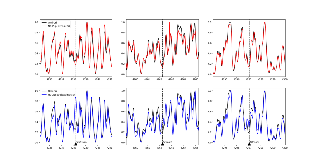
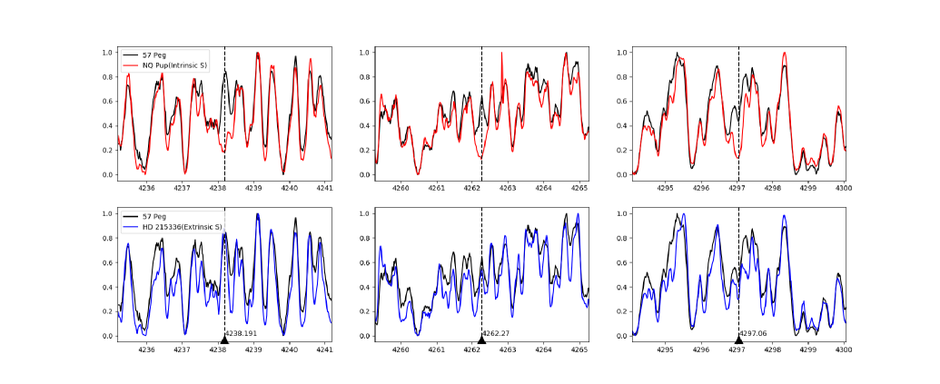
Figure 1: The spectral regions around the Tc I $\lambda$ 423.82 nm (left column), 426.23 (middle column), and 429.71 lines (right column). The star $o$1 Ori (black line) is compared to an intrinsic S star (NQ Pup; red line, first row) and to an extrinsic S star (HD 215336; blue line, second row), from HERMES spectra. Third and fourth rows: As in first and second rows, but for 57 Peg compared to the same intrinsic and extrinsic S stars.

Table 5: Abundances in the S stars $o$1 Ori (top panel) and 57 Peg (bottom panel). The column labeled $N$ gives the number of lines used to derive the corresponding abundances. The uncertainty listed in the $\log\epsilon_{X}$ column corresponds to the line-to-line scatter, whereas the one listed in column [X/Fe] is the root mean square of the former value and the uncertainty propagating from the model-atmosphere uncertainties, as estimated for V915 Aql by Shetye et al. (2018; their Table 8). V915 Aql has atmospheric parameters similar to those of $o$1 Ori and 57 Peg.

$o$1 Ori
MARCS model:
$T_{\rm eff}=3500$ K, $\log g=0.0$, [Fe/H] = -0.50, C/O = 0.50, [s/Fe]= 0.00
$Z$	X	$\log\epsilon_{X}$	[X/H]	[X/Fe]	$N$
6	C	$8.06$	-0.37	$\phantom{-}0.13$
7	N	$7.4$	-0.4	$0.07\pm 0.63$
26	Fe	$7.0\pm 0.13$	-0.5	$\pm 0.16$	12
39	Y	$1.8\pm 0.00$	-0.41	$0.09\pm 0.00$	2
40	Zr	$2.45\pm 0.07$	-0.13	$0.37\pm 0.07$	2
41	Nb	$1.02\pm 0.17$	-0.44	$0.06\pm 0.17$	4
56	Ba	$1.8\pm 0$	-0.4	$0.12\pm 0.10$	1
60	Nd	$1.0\pm 0$	-0.4	$0.08\pm 0.20$	2
57 Peg
MARCS model:
$T_{\rm eff}=3400$ K, $\log g=1.0$, [Fe/H] = 0.00, C/O = 0.50, [s/Fe] = 0.00
$Z$	X	$\log\epsilon_{X}$	[X/H]	[X/Fe]	$N$
6	C	$8.16$	-0.27	$-0.07$
7	N	$8.60$	0.77	$\phantom{-}0.97\pm 0.63$
26	Fe	$7.25\pm 0.14$	-0.25	$\pm 0.17$	13
39	Y	$1.95\pm 0.07$	-0.26	$0.04\pm 0.07$	2
40	Zr	$2.45\pm 0.21$	-0.13	$0.12\pm 0.21$	2
56	Ba	$2.0\pm 0$	-0.18	$0.07\pm 0.10$	1
60	Nd	$1.4\pm 0$	-0.02	$0.23\pm 0.20$	2
62	Sm	$0.85\pm 0.21$	-0.11	$0.14\pm 0.21$	2

5.2 The star $o$1 Ori (= HD 30959)

The star $o$1 Ori is peculiar in many respects. First, it is one of the few S stars with a direct detection of the WD companion from the International Ultraviolet Explorer (IUE; Ake & Johnson, 1988; Johnson et al., 1993). However, $o$1 Ori is also Tc-rich (Smith & Lambert, 1988, and bottom panel of Fig. 1), and as concluded by Ake & Johnson (1988), is clearly something of an anomaly in that it shows Tc lines and at the same time also hosts a WD companion, and could therefore be considered as an extrinsic S star. Simple considerations about the implied time scales (as explained below) make it more likely however that $o$1 Ori is a unique example of an intrinsic–extrinsic S star. In other words, this star must have recently entered the thermally pulsing AGB phase responsible for the Tc production, adding to the possible former s-process pollution from the now extinct AGB companion.

Since the half-life of ⁹⁹Tc, the isotope of Tc involved in the s-process, is $2.11\times 10^{5}$ yr, the presence of Tc on the stellar surface indicates that less than $10^{6}$ yr (i.e., a few half-lives) have elapsed since the last episode of Tc deposition on the surface. This constraint must be compared to the cooling time of $10^{8}$ yr for a white dwarf with $T_{\rm eff}=22\,000$ K (Salaris et al., 2013), as observed for $o$1 Ori. As these time scales are mutually incompatible, there is no possibility that the Tc now present on the M/S star (star intermediate between M- and S-spectral types) was transferred from the companion while it was still an AGB star. The location of $o$1 Ori in the Hertzsprung-Russell diagram, just at the onset of the thermally pulsing AGB (see Fig. 6 of Van Eck et al., 1998, confirmed by Gaia DR2, since the Hipparcos and Gaia DR2 parallaxes are mutually consistent: $\varpi=6.0\pm 0.9$ and $6.2\pm 0.4$, respectively), confirms the intrinsic nature of $o$1 Ori, that is, it is an S star on the TP-AGB capable of producing Tc in its interior and bringing it to the surface. The question remains however as to the origin (intrinsic or extrinsic) of the s-process enhancement which confers $o$1 Ori its distinctive status as an M/S star. An important clue in that respect comes from the Nb/Zr chronometer (Neyskens et al., 2015; Karinkuzhi et al., 2018), and from the orbital elements. In particular, is the system close enough to make the s-process pollution through mass transfer efficient?

To address the first question (intrinsic vs. extrinsic s-process), a basic abundance analysis of $o$1 Ori was performed, following the guidelines presented in Shetye et al. (2018), using the same iron and s-process lines, and the same procedure to select the model parameters among the large MARCS grid of S-star model atmospheres (Van Eck et al., 2017). The adopted model parameters for $o$1 Ori are listed in Table 5, and these parameters have been validated by the good match between observed and synthetic spectra around CH, Fe, and Zr lines. Figure 2 for instance illustrates this good match around a Zr I line.

Table 5 presents the abundances derived in $o$1 Ori for elements C, N, Fe, Y, Zr, Nb, Ba, and Nd. The specific MARCS model atmosphere selected for $o$1 Ori is validated a posteriori by the agreement between the [Fe/H] and [s/Fe] values for the adopted MARCS model and those derived from the detailed abundance analysis (more precisely, they differ by less than one step in the model grid for both [Fe/H] and [s/Fe]). Comparing the [Nb/Fe] and [Zr/Fe] abundances in $o$1 Ori with those observed in extrinsic and intrinsic S stars (Neyskens et al. 2015; also Fig. 14 of Karinkuzhi et al. 2018; Fig. 15 of Shetye et al. 2018) very clearly points towards an intrinsic origin of the $o$1 Ori s-process abundances. The small [Nb/Fe] value indeed indicates that ⁹³Zr has not yet had time to decay into the only stable Nb isotope, ⁹³Nb. Overall, the overabundance in s-process elements in $o$1 Ori is very moderate, with even some negative [X/Fe] values.

As far as the latter question (regarding the efficiency of s-process pollution through mass transfer) is concerned, the answer may come from the knowledge of $o$1 Ori orbital elements. It has been very difficult however to extract an orbital signal from the long-term radial-velocity monitoring, because the amplitude of variations is small (2 to 3 km s^-1) and there seems to be some velocity jitter (Fig. 3). This jitter could be associated with the envelope semi-regular pulsations with periods of 30.8 and 70.7 d, and amplitudes of 0.047 and 0.046 mag, respectively (Tabur et al., 2009). Using Eq. 5 of Kjeldsen & Bedding (1995) rewritten as Eq. 6 of Jorissen et al. (1997) to relate photometric and radial-velocity jitter, a radial-velocity amplitude of 0.75 km s^-1 is predicted to be associated with a photometric visual amplitude of 0.047 mag (adopting $T_{\rm eff}=3500$ K for $o$1 Ori; Table 5), in reasonable agreement with the data (bottom panel of Fig. 3).

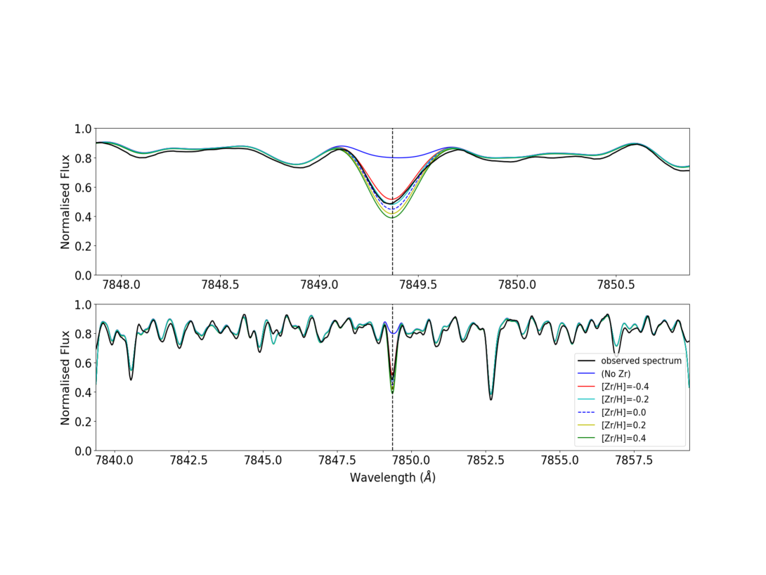
Figure 2: Illustration of the quality of the match between observed and synthetic spectra obtained for the extrinsic S star $o$1 Ori around the Zr I line at 7849.37 Å. The upper panel presents a $\pm\leavevmode\nobreak\ 3\leavevmode\nobreak\ \AA$ zoom.

An orbital solution may be obtained only after discarding data points obtained prior to 2012.7 (red crosses on Fig. 3). Even after this however, the $O-C$ residuals remain large ($\sigma(O-C)=0.44$ km s^-1; bottom panel of Fig. 3). The mass function is indeed the second smallest of those reported in Table 4, at $(2.7\pm 0.2)\times 10^{-5}$ M_⊙. As we show below, this small mass function is very likely due to a small inclination angle on the plane of the sky.

Ake & Johnson (1988) fit the IUE spectrum of $o$1 Ori B with a WD model of $\log g=8$, which according to Burleigh et al. (1997) corresponds to a mass of 0.65 M_⊙ and a radius of 0.014 R_⊙ for the WD (however, Ake & Johnson 1988 do not exclude that the gravity might be slightly larger, with $\log g=8.5$ then resulting in a mass of 0.96 M_⊙). Moreover, Cruzalèbes et al. (2013) have performed a detailed analysis of $o$1 Ori using AMBER/VLTI data. They obtained an angular diameter of $9.78\pm 0.10$ mas for that star, which, combined with the Gaia DR2 (DR2; Gaia Collaboration et al., 2016, 2018) parallax of $6.2\pm 0.4$ mas, yields a radius of $170\pm 14$ R_⊙. Combining this radius with the effective temperature of 3500 K gives a luminosity of 3900 L_⊙. Given the [Fe/H] $=-0.5$ metallicity of $o$1 Ori (Table 5), the above parameters locate the star on the evolutionary track of a 2 – 2.5 M_⊙ star according to Fig. 16 of Shetye et al. (2018). Inserting these masses and their uncertainties into the orbital mass function, we obtain an inclination on the order of only $\sim 3.7^{\circ}-5.7^{\circ}$ on the plane of the sky.

Combining the above mass estimates with the orbital period of 575 d (Table 4), one finds a relative semi-major axis in the range 1.9 – 2.0 au or 404 R_⊙. The corresponding Roche radius around the giant component is then on the order of 184 – 235 R_⊙, corresponding to a filling factor on the order of 72 – 92% for the observed radius of $170\pm 14$ R_⊙. Orbital and diameter data thus indicate that $o$1 Ori is a detached system, possibly with a large filling factor. Ellipsoidal variations are not expected though, since the system appears to be seen almost face-on. However, in this case, a noncircular stellar disk could be detected by interferometry, using three non-aligned telescopes. The closure-phase parameter (CSP) may be used to measure the deviation from centrosymmetry of the stellar surface brightness distribution, as done by Cruzalèbes et al. (2015). The CSP relies on the triple product of the complex visibilities recorded by the three telescopes; its exact definition is beyond the scope of this paper, and we refer the interested reader to the paper by Cruzalèbes et al. (2014). The closure-phase parameter is equal to $0^{\circ}$ or $180^{\circ}$ for a central-symmetric surface brightness distribution. In $o$1 Ori, there is a small deviation from centrosymmetry (CSP $=8.1^{\circ}\pm 0.8^{\circ}$ instead of $0^{\circ}$ in the central-symmetric case). However, this level of asymmetry could also be caused by the convective pattern at the surface of this giant star (see Cruzalèbes et al., 2014; Paladini et al., 2014, for a discussion of convective vs. tidal asymmetries in giant stars). The CSP value for $o$1 Ori indeed lies at the expected position along the sequence of increasing convective asymmetries with increasing pressure scale-heights along the giant branch (see Figs. 4 and 6 of Cruzalèbes et al., 2015). Therefore, it is likely that $o$1 Ori shows no sign of tidal deformation, meaning that its Roche-filling factor must be closer to 72% than to 92%; hence, the most likely masses are those corresponding to the filling factor of 72%, namely $M_{\rm S}=2.5$ M_⊙ and $M_{\rm WD}=0.65$ M_⊙.

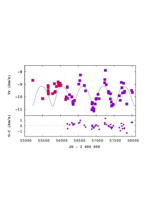
Figure 3: The tentative orbit of $o$1 Ori, based on the magenta square points.

5.3 HD 98839 = 56 UMa

For HD 98839 (=56 UMa), we improve upon the orbit published by Griffin (2008a). Thanks to 25 new HERMES measurements spanning the years 2009 – 2016 as listed in Table 2, a full orbital cycle has now been covered for this barium star with an orbital period of $45.1\pm 0.3$ yr, one of the longest among barium and extrinsic S stars.

An offset of +0.6 km s^-1  was applied to these HERMES measurements to put them in agreement with those used by Griffin for his orbital solution. Nevertheless, the systemic velocity listed in Table 4 has been converted back into the HERMES/IAU system to ensure consistency with the other orbital solutions. In our orbital solution (shown in Fig. 26), we did not include measurements older than JD $2\;440\;000$, because they degrade the orbit quality.

5.4 HD 134698

HD 134698 has a very large eccentricity ($e\sim 0.95$), and it was not possible to converge to a solution taking into account all the old CORAVEL data points, as shown in Fig. 31, because the data sampling does not cover the periastron passage sufficiently well. The solution obtained is very sensitive to the choice of the CORAVEL points used to compute the orbit (choices different from the one displayed in Fig. 31 generally lead to eccentricities even closer to one), which is a sign that the solution is not robust.

5.5 HD 196673

HD 196673 is a visual double star (WDS 20377+3322) with a separation varying between 2.5″ in 1828 and 3.2″ in 2014. According to the Gaia Data Release 2 (Gaia Collaboration et al., 2016, 2018) the B component is about one magnitude fainter than the barium star, and their $Bp-Rp$ are similar (1.275 and 1.187 for A and B, respectively), as are their parallaxes ($\varpi=1.62\pm 0.03$ mas). This indicates that AB is a pair of red giants, separated by $\sim 1850$ au. Assuming a mass of 1.5 M_⊙ for both stars leads to an orbital period of $5\times 10^{4}$  yr. One radial-velocity measurement of HD 196673B has been obtained (-25.5 km s^-1; Table 2), close to the systemic velocity of the Aa spectroscopic pair (-24.2 km s^-1; Table 4), further confirming that the visual pair is physical.

5.6 T Sgr = HD 180196

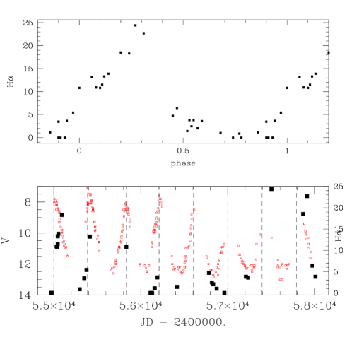
Figure 4: Bottom panel: Light curve for the S star T Sgr (small red open squares on bottom panel), from the Association of French Variable Star Observers (AFOEV). The vertical dashed lines mark the light maxima, either directly identified on the light curve (the first four) or inferred from the GCVS period 394.7 d. The strength of the Balmer H$\alpha$ emission line peak value normalised with respect to the continuum) is represented as solid open squares to be read off the right scale. Top panel: Balmer H$\alpha$ line strength as a function of the photometric phase.

Figure 5: Cross-correlation functions of the S star T Sgr (using mask F0) ordered according to (fractional) photometric phase, counted in cycles (as labelled in the right margin) since the light maximum at JD 2454611 (see Fig. 4). The vertical dashed lines mark the two peaks appearing in the Mira spectrum between phases -0.1 and 0.3, at velocities -13 and +7 km s^-1. These peaks exhibit no noticeable orbital drift over the 9 years covered by the radial-velocity monitoring. The noisy CCFs between phases 0.5 and 0.6 (represented in red, and corresponding to the Mira minimum light) reveal a broad single peak, most likely belonging to the F companion, centered around -2 km s^-1, and with a rotational broadening of about 25 km s^-1.

The Tc-rich S star T Sgr has been included in the monitoring because the star is known to have a composite spectrum, with a F4 IV companion becoming visible near minimum light (Herbig, 1965; Culver & Ianna, 1975), and we hoped to detect the velocity drift associated with the orbital motion. However, as we explain below, despite 9 years of monitoring no such drift has been clearly detected, suggesting that the pair must be relatively far apart.

T Sgr is a Mira variable with a period of 394.7 d according to the General Catalogue of Variable Stars (v. 5.1; Samus’ et al., 2017). This period is confirmed by the AFOEV which detected light variations with a period varying between 377 d (cycle 3) and 446 d (cycle 2) during the time-span of the HERMES monitoring campaign (bottom panel of Fig. 4). The photometric phase was computed with an origin at JD 2454611, and using either the contemporaneous period (when it could be measured from the photometric data, for cycles 1–4) or the GCVS period of 395 d (cycles 5–8). The photometric phase is listed again in the right margin of Fig. 5, which shows the series of CCF obtained with a F0 template, ordered according to the photometric phase. Along the eight photometric cycles covered, the CCFs have stayed remarkably similar at any given phase, thus showing no sign of orbital drift.

The Mira has a shock wave traveling through its photosphere around maximum light. This shock wave manifests as line doubling (between fractional phases -0.1 to 0.3; Fig. 5), a well-studied behavior known as the Schwarzschild scenario (see Alvarez et al. 2000 and Jorissen et al. 2016 for an illustration of that scenario at work in Mira variables). The red component, corresponding to infalling matter, is the only one present during fractional phases 0.7 – 0.9, and gives way to an increasingly strong blue component, corresponding to rising matter. In T Sgr, these two peaks have velocities of about -13 and +7 km s^-1  (Table 6). At the same time, H$\alpha$ in emission gets stronger and stronger (top panel of Fig. 4). In that figure, the number characterizing H$\alpha$ emission is simply $[I_{\rm max}(H\alpha)-I(\rm{continuum})]/I(\rm{continuum})$.

Table 6: The radial velocities of the F and Mira components of the T Sgr system as a function of the photometric phase $\phi$, along with the $\sigma$ of the CCF. The last columns list the velocities of the two peaks associated with the shock wave traveling in the Mira photosphere.

JD	$\phi$	$Vr$ (F)	$\sigma$(CCF)	$Vr1$ (Mira)	$Vr2$ (Mira)
		(km s-1)	(km s-1)	(km s-1)	(km s-1)
2455297.71	1.77	$-0.8\pm 0.3$	16.3	-	-
2455413.57	2.06	-	-	$-13.9\pm 0.1$	$8.3\pm 0.1$
2456159.46	3.86	-	-	-	$6.9\pm 0.2$
2456190.45	3.94	-	-	$-12.9\pm 0.3$	$6.4\pm 0.2$
2456416.70	4.52	$-1.8\pm 0.4$	14.6	-	-
2456784.70	5.45	$-2.7\pm 0.6$	20.5	-	-
2456817.65	5.54	$-3.2\pm 0.4$	19.0	-	-
2456832.61	5.57	$-4.2\pm 0.4$	15.0	-	-
2457208.54	6.53	$-3.8\pm 0.5$	15.0	-	-
2457867.75	8.20	-	-	$-13.7\pm 0.1$	$8.7\pm 0.1$
2458008.39	8.55	$-2.7\pm 0.5$	15.8	-	-

Around phase 0.5 (minimum light), these double peaks give way to a broad single peak, and this feature is especially visible when performing the correlation of the observed spectrum with a F0 mask. The corresponding velocities are listed in Table 6, which reveals a drift, but its significance is weakened by the broadness of the CCF (on the order of $\sigma\sim 15$ km s^-1, associated with a rotational velocity $V_{\rm rot}\sin i\sim 25$ km s^-1). The Mira velocity peaks do not confirm this drift, although a supplementary complication here comes from the fact that the shock-wave velocity may vary from cycle to cycle.

We note as well that the F-star velocity falls almost exactly at mid-range between the two Mira peaks, which is surprising; either the two stars are now going through a conjunction on a very long orbit, or the velocity amplitude of their orbit is small (a few km s^-1), or indeed the broad CCF seen at minimum light is not at all related to the F star.

5.7 HD 218634 = 57 Peg

The preliminary orbit of the S star 57 Peg (HD 218634) stands out, with its orbital period of the order of 500 yr (Table 4 and Fig. 41), the longest period known so far for a chemically peculiar red giant, and probably even among spectroscopic binaries as a whole (Griffin, 2008a). To better constrain it, it was necessary to add the old measurements from Griffin & Peery (1974). The period is not well constrained, and we do not exclude however that the orbital period could turn out to be shorter (100 yrs?; see the dashed line in Fig. 41) when evaluated with measurements spanning a longer time interval.

The Tc-poor star 57 Peg (see bottom panel of Fig. 1) is special in many respects. First, it has a rather high luminosity ($M_{\rm bol}=-4.3$, with a small uncertainty on its Hipparcos parallax $\sigma_{\varpi}/\varpi=0.21$; Hipparcos and Gaia DR2 parallaxes for 57 Peg are consistent with each other, with the Gaia parallax being only twice more precise: $\sigma_{\varpi}/\varpi=0.10$), and it falls along the $Z=0.2$ evolutionary track of a 3 M_⊙ star (Fig. 6 of Van Eck et al., 1998). Second, according to the detailed analysis of its UV colours presented in the Appendix of Van Eck et al. (1998), it has a composite spectrum with an A6V companion instead of the WD companion expected for extrinsic S stars in the framework of the binary paradigm. Adopting a mass of 1.9 M_⊙ for such an A6V companion yields a $Q$ value of 0.286 M_⊙ (with $Q=M_{\rm A}^{3}/(M_{\rm S}+M_{\rm A})^{2}$), assuming a mass of 3 M_⊙ for the S star. Incidentally, the S star primary must have evolved faster and should therefore be more massive than 1.9 M_⊙, which is consistent with its position along the 3 M_⊙ track in the HR diagram. Despite the fact that the orbit is not yet fully constrained, it yielded a mass function of $f(M_{\rm S},M_{\rm A})=0.38\pm 0.22$ M_⊙, compatible (within the error bars) with the above-predicted value for a 1.6 M_⊙ companion (since $\sin^{3}i=f(M_{\rm S},M_{\rm A})/Q$, and therefore $f(M_{\rm S},M_{\rm A})$ should be smaller than $Q$). However, a WD companion with a mass of 0.7 M_⊙, which would yield $Q=0.025$ M_⊙, seems incompatible with the observed mass function and the condition $f(M_{\rm S},M_{\rm A})\leq Q$. All evidence therefore suggests that the companion is on the main sequence. The star 57 Peg thus adds to the small set of Tc-poor S stars (HD 191589, HDE 332077) with a main sequence companion (Jorissen & Mayor, 1992; Ake & Johnson, 1992; Ake et al., 1994; Jorissen et al., 1998).

Faced with such strong evidence, possibilities to resolve this puzzle within the framework of the binary paradigm include scenarios where (i) 57 Peg is a triple system (S+A6V+WD), (ii) the companion is an accreting WD mimicking a main sequence spectrum, (iii) 57 Peg is an intrinsic (Tc-rich) rather than a Tc-poor S star, and finally (iv) 57 Peg is not an S star at all.

Possibility (i) is incompatible with the long-period orbit of the system, since a triple system needs to be hierarchical to be stable, with a period ratio on the order of ten. Since the 500 yr orbit is that of the main-sequence companion (as derived from the mass function), a 5000 yr orbit is implied for the WD companion (a 50 yr orbit is not possible, since it would be detected first, having a larger velocity amplitude). However, a 5000 yr orbit (corresponding to $1.8\times 10^{6}$ d) would never yield large enough pollution levels to transform the accretor into an extrinsic S star, since the longest orbital periods among our representative samples of extrinsic stars do not exceed $4\times 10^{4}$ d (see also Fig. 15 showing how [s/Fe] decreases with increasing orbital periods).

Possibility (ii) is neither supported by the mass function, which calls for a genuine A6V star rather than a rejuvenated WD, nor the IUE SWP spectrum, which carries no sign of binary interaction (no C IV $\lambda$ 155.0 nm emission for instance).

Possibility (iii) is refuted by Fig. 1, which clearly demonstrates the Tc-poor nature of 57 Peg, based on a HERMES spectrum around the Tc I $\lambda$ 423.82 nm, 426.23, and 429.71 lines.

Possibility (iv) – that 57 Peg is not an S star – was already suggested by Smith & Lambert (1988). This hypothesis can be tested from an abundance analysis of the s-process elements in 57 Peg. For this purpose, we use an HERMES spectrum of 57 Peg obtained on September 6, 2009 (JD 2455080.640), with a signal-to-noise ratio of 150 in the $V$ band. The atmospheric parameters of 57 Peg were derived following the method described by Van Eck et al. (2017) and Shetye et al. (2018). The adopted model parameters are listed in the bottom panel of Table 5. The abundance analysis has been performed using the same iron and s-process lines as in Shetye et al. (2018). We note especially that the lines used were located far enough in the red not to be contaminated by light from the A-type companion. Figure 6 presents the good match between the synthetic and observed spectra around a Zr I line. Table 5 reveals that all the heavy elements studied have an abundance compatible with the solar-scaled value. The error bars quoted in column [X/Fe] of that table include, on top of the line-to-line scatter, the uncertainty propagating from the model-atmosphere uncertainties. The latter was estimated by Shetye et al. (2018; their Table 8) for the S star V915 Aql and applied here to 57 Peg, since both stars have similar atmospheric parameters (same $T_{\rm eff}$ but $\log g$ differing by 1 dex).

There is however a surprising N overabundance (larger than expected after the first dredge-up, if taken at face value; on that topic, see also Karinkuzhi et al., 2018). Therefore, our conclusion regarding 57 Peg is that this star has been misclassified as an S star, in line with the suggestion by Smith & Lambert (1988).

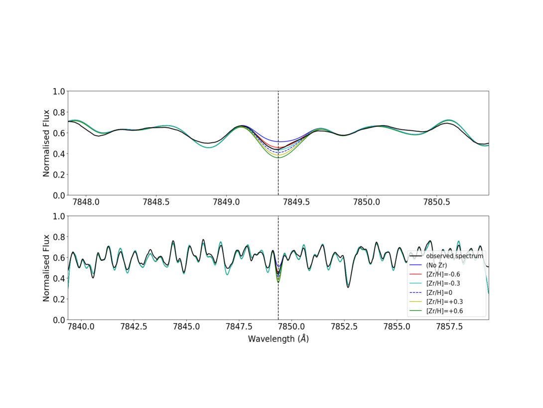
Figure 6: As in Fig. 2 but for 57 Peg.

6 The eccentricity–period diagram

With the addition of the new HERMES orbits to the existing sample (Jorissen et al., 1998; Van der Swaelmen et al., 2017), the number of giant barium and S stars with orbital elements available now amounts to 105 systems (36 strong Ba, 37 mild Ba, and 32 S stars). In the remainder of this paper, we analyze this rich data set, starting with the $e-P$ diagram (Fig. 7). This diagram reveals distinctive features that may be used as benchmarks for binary-evolution models:

• the upper left threshold (represented by the dashed line in panel (c) of Fig. 7), due to tidal evolution or periastron mass transfer;

• the lower right gap (represented by the hatched area in Fig. 7), survival from initial conditions observed in young binaries like pre-main sequence stars;

• the existence of two populations: a population with (nearly) circular, short-period ($P<10^{3}$ d) orbits (almost exclusively found among strong barium stars), and a population of eccentric systems with intermediate ($10^{3}\leq P({\rm d})\leq 10^{4}$) and very long periods ($P>10^{4}$ d).

With all orbits now available, including the very long-period ones, we can state that the longest orbital period where s-process pollution through mass transfer may produce an extrinsic star is about $4\times 10^{4}$ d ($\sim 110$ yr), since no system with a period longer than this value is found in our samples. This period however is the post-mass-transfer value, which certainly differs from the initial value. This maximum period provides an interesting constraint for binary mass-transfer models, which often predict the possibility of forming extrinsic systems with even longer periods (as long as a few $10^{5}$ d; see Abate et al., 2015b, 2018, and references therein).

Extrinsic S stars (Panel d of Fig. 7) do not add new features or structure in the $e-P$ diagram; they confirm the division of Ba stars in two populations in the $e-P$ diagram. The maximum eccentricity at a given period is similar for barium and S stars (if one excepts the presence of two barium stars at $P\sim 10^{4}$ d with large eccentricities – $e>0.9$, with no equivalent among S stars, but this may result from small-number statistics). Extrinsic S stars are thus fully identical to barium stars in terms of their orbits.

The population of (almost) circular barium stars with $P<1000$ d is likely to contain objects that were circularized by tidal effects while the current barium star was ascending the first giant branch (supposing that most barium stars are currently located in the red-giant clump, as suggested by the analysis of their Hertzsprung-Russell diagram; Escorza et al., 2017). This circularisation process is posterior to and independent from the mass-transfer process. We justify the above statement by the fact that S stars, which are still on the RGB, are not yet fully circularized in the same period range, as indicated by the large clump of S stars observed around $P\sim 700$ d and $e\sim 0.08$. A similar argument holds for the $e-P$ diagram of post-AGB and dwarf barium stars, which also include short-period noncircular systems (Oomen et al., 2018; Escorza et al., 2019). One may actually wonder why these post-AGB, dwarf-barium, and S systems with short orbital periods are not circularized as they have hosted a large AGB star in the past. Several authors argued that an as yet not fully identified process (e.g. periastron mass transfer, tidal interaction with a circumbinary disk, or a momentum kick associated with the white-dwarf formation) must have been at work during the mass-transfer process to counteract the circularisation process and to pump the eccentricity up (Soker, 2000; Izzard et al., 2010; Dermine et al., 2013).

We stress moreover that the population of (almost) circular barium stars with $P<1000$ d is almost absent among mild barium stars (with the exception of HD 77247 and HD 218356). Therefore, there must be a link between the mass-transfer properties and the resulting s-process overabundances to account for the near absence of short-period systems among systems with mild s-process overabundances. This is further discussed in Sect. 9. As a corollary, we note that HD 199939, with $P=585$ d and $e=0.28$, is an outlier among strong barium stars, having a large eccentricity for its period (panel b of Fig. 7). Its orbital elements were obtained by McClure & Woodsworth (1990), and a closer look at their orbital solution does not reveal any anomaly (like the presence of a third companion) that could account for its outlying nature. Finally, we stress that the segregation between mild and strong barium stars, used to draw panels (a) and (b) of Fig. 7, although initially based on the Warner visual index of the strength of the Ba II line (Warner, 1965), is generally confirmed by a detailed abundance analysis (as further discussed in Sect. 9). Adopting [La/Fe] and [Ce/Fe] values of 1 dex as threshold between mild and strong barium stars, we find only two stars that need to be reclassified: HD 183915 (from mild to strong), and NGC 2420-173 (from strong to mild; see Table 8).

The CH and CEMP stars (panel (e) of Fig. 7 from Jorissen et al., 2016), which are the low-metallicity counterparts of barium stars, behave exactly as barium stars, in particular regarding the circular nature of most of the short-period orbits. The only notable difference is the presence of a very short-period ($P<10$ d) orbit, but this one is associated with a dwarf carbon star. The few CH/CEMP systems falling in the low-eccentricity gap probably have inaccurate values for the eccentricity, as discussed by Jorissen et al. (2016).

The correlation between abundances and location in the $e-P$ diagram is discussed in Sect. 9.

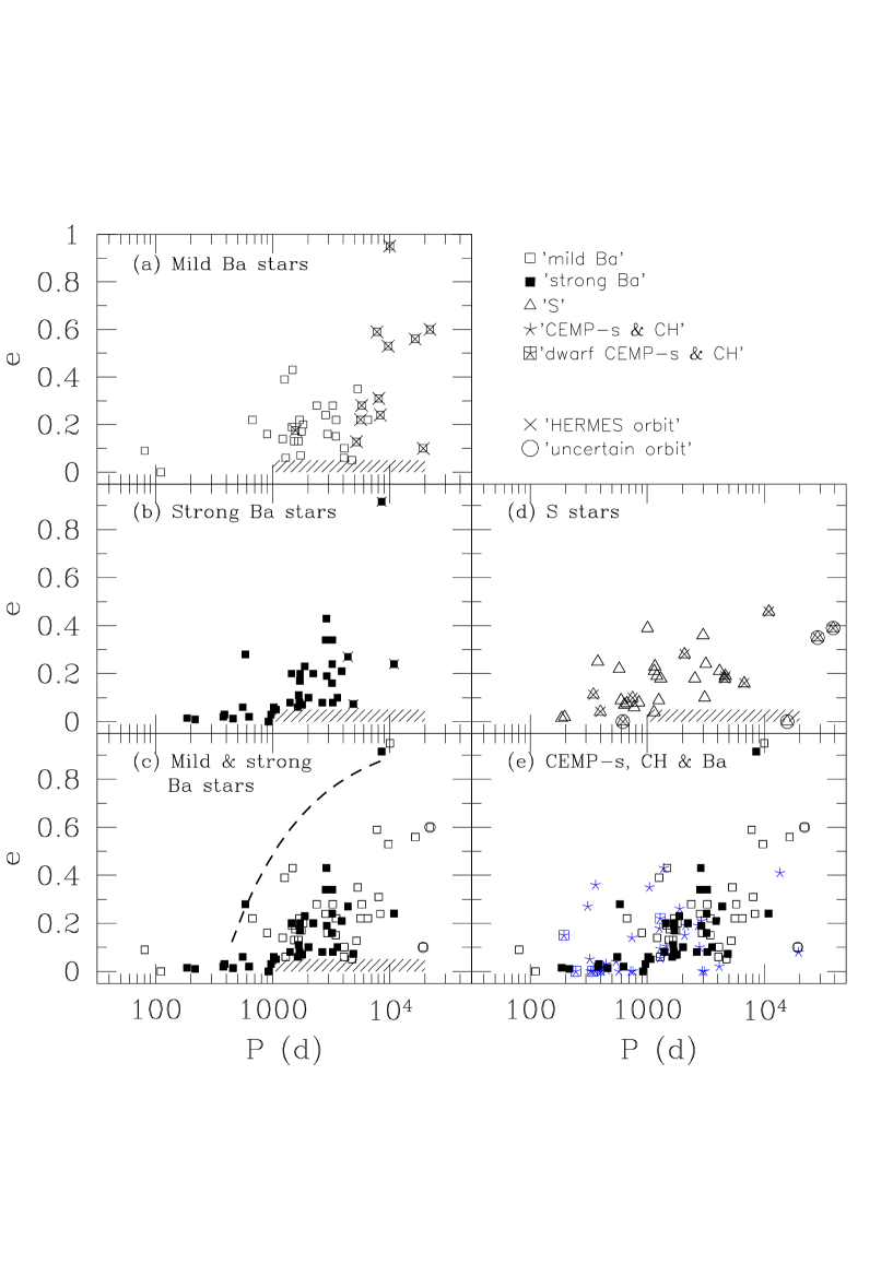
Figure 7: Eccentricity–period diagrams for various samples. The meaning of the various symbols is given in the upper right panel. (a) Mild barium stars; (b) Strong barium stars; (c) Mild (open squares) and strong (filled squares) barium stars plotted together. The dashed line corresponds to the upper envelope of the data points, well represented by the condition 143 R${}_{\odot}=R_{\rm Roche}=A\;(1-e)\;[0.38+0.2\log(M_{\rm Ba}/M_{\rm WD})]$, corresponding to RLOF occurring at periastron for a star of radius 143 R_⊙. $A$ is the semi-major axis of the orbit, linked to the orbital period $P$ through the third Kepler law, adopting component masses of $M_{\rm Ba}=2$ M_⊙ and $M_{\rm WD}=0.65$ M_⊙; (d) S stars (triangles). The S star HD 184185, with $P\sim 15723$ d and $e\sim 0$, falls in the low $e$ – long $P$ gap (represented by the hatched area), probably as a consequence of its still-uncertain orbital parameters; (e) As in (c), adding CEMP-s and CH stars (blue 5-branch crosses; squared crosses correspond to carbon dwarfs from Jorissen et al., 2016). The dwarf CEMP star HE 0024-2523 with an orbital period of 3.4 d falls outside the graph boundaries.

7 Mass distribution of barium stars and their white dwarf companions

7.1 Methods

In previous papers, we obtained the mass (Escorza et al., 2017) and mass-ratio (Van der Swaelmen et al., 2017) distributions of barium stars. The formerly obtained mass distribution however had only a statistical value, since it was based on the average metallicity of barium stars ([Fe/H] = -0.25), rather than on their individual values. Masses derived from the comparison between evolutionary tracks and location in the Hertzsprung-Russell diagram (HRD), as done by Escorza et al. (2017), are sensitive to the metallicity and therefore do require prior derivation of individual metallicities to reach the ultimate accuracy. Metallicities of barium stars have now been collected from the literature, and when not available were derived from high-resolution HERMES spectra (Raskin et al., 2011). The derivation of the atmospheric parameters was performed as described in Karinkuzhi et al. (2018), and the luminosities as described in Escorza et al. (2017). The Fe line list used is given in Table 10, with metallicities in Table 8. Masses are then derived by matching the position of the barium star in the HRD with STAREVOL evolutionary tracks of the same metallicity (Van der Swaelmen et al., 2017; Escorza et al., 2017). In case of ambiguities, when tracks of different masses pass close to the location of the star in the HRD, we use a statistical criterion that compares the speed of evolution along the different tracks at a given location in the HRD and select the slowest one (see the discussion around Eqs. 2 and 3 in Escorza et al., 2017). The resulting metallicities and masses are listed in Table 8, along with heavy-element abundances derived as outlined by Karinkuzhi et al. (2018).

We used Gaia DR2 parallaxes (Gaia Collaboration et al., 2018) to derive the distances and luminosities following the method outlined in Escorza et al. (2017). Gaia DR2 parallaxes result exclusively from single-star solutions. As shown by Pourbaix & Jorissen (2000), the absence of binary processing by the astrometric pipeline could lead to incorrect parallaxes only when the orbital motion with a period close to 1 yr confuses the parallactic motion. In our sample, only two stars match this criterion (DM $-64^{\circ}$4333, HD 24035; see Table 8) and therefore their masses listed in Table 8 are subject to caution. Nevertheless, the corresponding WD masses for these two stars do not look peculiar.

The distribution of mass ratios ($q=M_{\rm WD}/M_{\rm Ba}$) is obtained from the distributions of primary masses $M_{\rm Ba}$ and mass functions $f(M_{\rm Ba},M_{\rm WD})$ under the assumption that the orbital inclination is randomly distributed according to $g(i)=\sin i$, since

$$f(M_{\rm Ba},M_{\rm WD})=\frac{M_{\rm WD}^{3}}{(M_{\rm Ba}+M_{\rm WD})^{2}}\;\sin^{3}i=M_{\rm Ba}\frac{q^{3}}{(1+q)^{2}}\;\sin^{3}i.$$ (1)

To derive the distribution of $q$, we use the method designed by Boffin et al. (1992), which relies on a Richardson-Lucy deconvolution and has proven to be very robust and reliable (see Boffin et al., 1993; Cerf & Boffin, 1994; Pourbaix, Jancart, & Boffin, 2004; Boffin, 2010, 2012; Van der Swaelmen et al., 2017).

In principle, the distribution of mass ratios $q$ has only a statistical meaning and it is difficult to attribute a given mass ratio to a specific system. Nevertheless, this may be attempted under two different hypotheses: (i) finding the most peaked distribution of the companion masses, as expected if they are WD companions, or (ii) finding the distribution corresponding to a constant $Q=M^{3}_{\rm WD}/(M_{\rm Ba}+M_{\rm WD})^{2}$ value, separately for mild and strong barium stars. The two methods are discussed in turn in what follows.

Since $M_{\rm WD}=q\times M_{\rm Ba}$, the most peaked $M_{\rm WD}$ distribution may be obtained by performing the $q\times M_{\rm Ba}$ product with $q$ and $M_{\rm Ba}$ sorted in opposite order (i.e., largest $q$ combined with smallest $M_{\rm Ba}$, and so on). The number of occurrence of each $q$ in this list of products is fixed by its frequency distribution $f(q)$ (Fig. 11) multiplied by the sample size of $M_{\rm Ba}$. To limit the round-off errors due to the small sample size (only $N=24$ strong barium stars), the sample size has been multiplied by ten, meaning that each individual $M_{\rm Ba}$ value appears ten times in the list, while each $q$ bin value appears $f(q)\times N\times 10$ times.

An alternative method to derive the mass-distribution of WDs is based on the assumption of constant $Q=M^{3}_{\rm WD}/(M_{\rm Ba}+M_{\rm WD})^{2}$. Webbink (1988) showed that the distribution of $f(M_{\rm Ba},M_{\rm WD})\equiv Q\sin^{3}i$ known at the time for barium stars was compatible with a single value of $Q=M_{\rm Ba}\;q^{3}/(1+q)^{2}$. This correlation between the masses of the barium star and its WD companion is understandable since the more massive the barium star is, the more massive its companion had to be (and hence its WD progeny). Looking at the current sample, it appears that for the strong barium stars $Q$ is indeed sharply peaked at $0.057\pm 0.009$ M_⊙, whereas for mild barium stars the distribution of $Q$ may be approximated by a somewhat wider Gaussian ($0.036\pm 0.027$ M_⊙; Fig. 8). The good agreement between observed and modeled distributions is confirmed by a Kolmogorov-Smirnov test. A similar analysis on an earlier sample of barium-star orbits (Jorissen et al., 1998) yielded similar values ($0.049$ M_⊙ and $0.035$ M_⊙ for strong and mild barium stars, respectively). Considering the result that $Q$ is basically fixed (a very good approximation at least for strong barium stars), it will be possible to extract $M_{\rm WD}$ from $Q$ and $M_{\rm Ba}$ for each system.

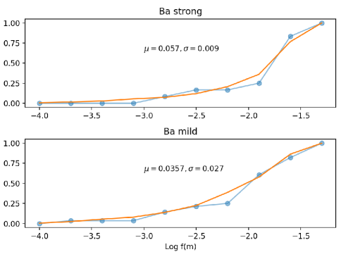
Figure 8: Cumulative mass-function distributions for mild and strong barium stars, as compared to those inferred from a Gaussian distribution of $Q=M_{\rm Ba}\;q^{3}/(1+q)^{2}$ (with the Gaussian parameters as mentioned in the figure: $\mu$ is the Gaussian average and $\sigma$ its standard deviation, both in M_⊙), convolved with random orbital inclinations.

7.2 Results

The mass distribution is shown in Fig. 9, separately for mild and strong barium stars. Mild barium stars exhibit a clear tail towards masses up to 5 M_⊙, whereas strong barium stars are restricted to about 3.5 M_⊙. Figure 10 confirms that if the threshold between mild and strong barium stars is set at 1 dex for both [La/Fe] and [Ce/Fe] (a reasonable value as revealed by Table 8), mild barium stars indeed include a tail of high-mass ($M>3$ M_⊙), high-metallicity ([Fe/H] $>-0.1$) stars. If this high-mass tail is removed, any correlation between mass and abundances disappears.

The statistical significance of the apparent difference between the mass distributions for mild and strong barium stars may be evaluated from a Kolmogorov-Smirnov test (e.g., Press et al., 1986). The maximum difference between the two cumulative frequency distributions amounts to 0.29 (bottom panel of Fig. 9). Considering that the samples comprise $m=30$ mild barium stars and $n=24$ strong barium stars, resulting in an effective sample size of $m\times n/(m+n)=13$, the observed difference translates into a significance level of 79%. This implies that the first-kind error of erroneously rejecting the null hypothesis that the two distributions are similar is 21%. The difference between the mass distributions of mild and strong barium stars – albeit not very significant – clearly originates from the presence of a high-mass tail among mild barium stars. The fact that in our previous paper (Fig. 14 of Escorza et al., 2017), this high-mass tail among mild barium stars was not as clear as here, rather than contradicting our present results, reveals the limitations of the analysis of that former paper, where the same metallicity for all barium stars was adopted. Similar claims that mild barium stars extend towards larger masses than strong barium stars were formerly put forward by Catchpole et al. (1977), Mennessier et al. (1997), and Jorissen et al. (1998).

Figure 9: Top panel: Mass distributions for mild (dashed lines) and strong (solid lines) barium stars. Bottom panel: Cumulative mass distributions. The maximum vertical difference between the two distributions amounts to 0.29.

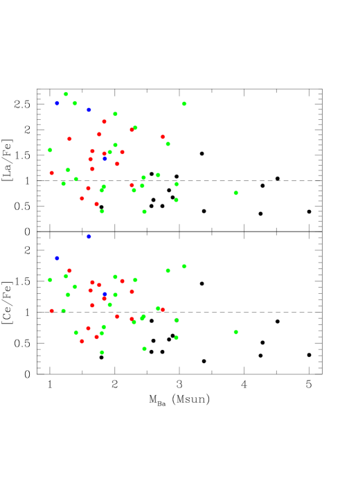
Figure 10: Relationship between barium-star masses and [La/Fe] and [Ce/Fe] abundances, color-coded according to metallicity: Blue ([Fe/H] $\leq-0.6$), red ($-0.6<$ [Fe/H] $\leq-0.3$), green ($-0.3<$ [Fe/H] $\leq-0.1$), and black ($-0.1<$ [Fe/H]).

Figure 11: Mass-ratio distributions for mild (bottom panel) and strong (top panel) barium stars. The dashed lines correspond to the $q$ distribution obtained from the Richardson-Lucy inversion (see text), whereas the solid line corresponds to the $q$ distribution rederived from the individual $M_{\rm Ba}$ and $M_{\rm WD}$ estimates (Table 8) under the assumption of a constant $Q$ (different for mild and strong barium stars).

The $q$ $(=M_{\rm WD}/M_{\rm Ba})$ distributions for mild and strong barium stars are shown in Fig. 11. The resulting $M_{\rm WD}$ distribution is shown in Fig. 12 under the most-peaked assumption, as explained in Sect. 7.1, and in Fig. 13 for the constant-$Q$ assumption.

The distributions of Fig. 12 are by construction strongly peaked (with the exception of a few non-physical ”WDs” around 0.2 and 0.45 M_⊙) at 0.6 – 0.7 M_⊙ for WDs around mild barium stars, and at 0.6 – 0.9 M_⊙ for WDs around strong barium stars. As expected, the distributions shown in Fig. 13 for the constant-$Q$ assumption are somewhat broader than the limiting cases displayed in Fig. 12, and the small-mass outliers have disappeared. The consistency of this WD mass distribution obtained under the assumption of a constant $Q$ is further checked by comparing in Fig. 11 the mass ratios $q$ obtained from these WD masses and the paired barium masses (as listed in Table 8), with the $q$ distribution obtained directly from the Lucy-Richardson inversion. Both $q$ distributions are in good agreement, as they differ only by the presence of sparsely populated bins in the Richardson-Lucy results (dashed lines in Fig. 11).

Another independent check of the WD masses obtained above may be performed for the few barium stars which were found to be astrometric binaries based on Hipparcos data (Pourbaix & Jorissen, 2000). A subsequent study (Jancart et al., 2005) assessed the quality of the astrometric orbital elements derived by Pourbaix & Jorissen (2000) and concluded that only HD 46407 (HIP 31205) and HD 101013 (HIP 56731) marginally satisfy the orbital quality checks (see their Table 5). Relevant data for these two systems are collected in Table 7, which reveals an agreement between the two mass values within $2\sigma$.

Moreover, in the case of HD 204075 ($\zeta$ Cap), the WD companion has been detected directly from its UV radiation, using the IUE satellite (Böhm-Vitense, 1980), and the mass estimated from the observed spectrum is of the order of 1 M_⊙, in perfect agreement with the ”constant-$Q$” value WD mass.

For the sake of completeness, Table 8 also lists HD 121447, although that star was not included in the luminosity determination using Gaia DR2 parallaxes. This star is suspected to be an ellipsoidal variable (Jorissen et al., 1995). The photometric analysis of the system has yielded masses of $1.6\pm 0.1$ M_⊙ and $0.6\pm 0.1$ M_⊙ for the barium star and its WD companion, respectively.

Table 7: WD masses derived from the astrometrically based $\sin i$ (Pourbaix & Jorissen, 2000) and from the assumption of constant $Q$. The error bars for the WD mass derived from astrometry correspond to the error propagation from the inclination. The column labeled ‘Ba’ lists whether the star is a mild (‘m’) or strong (‘s’) barium star.

HD	HIP	Ba	$M_{\rm Ba}$	$f(M)$	$i$	$M_{\rm WD}$
						($i$)	($Q$)
			(M⊙)	(M⊙)	(∘)	(M⊙)	(M⊙)
46407	31205	s	2.12	0.035	$80\pm 10$	0.71${+0.04\atop-0.02}$	0.78
101013	56731	s	1.65	0.037	$78\pm 26$	0.59${+0.18\atop-0.02}$	0.68

It is now possible to compare the masses of the WD companions of barium stars with field WDs. Current estimates for the average mass of the latter (represented by the red vertical dashed lines on Figs. 12 and 13) is $0.593\pm 0.002$ M_⊙ for DA WDs and $0.676\pm 0.014$ M_⊙ for DB WDs (Kleinman et al., 2013). The mass distribution of WD companions of barium stars appears to have a tail extending toward masses larger than those of field WDs. Moreover, there is a hint that WDs around strong barium stars may be more massive on average than WDs around mild barium stars. This trend is relatively significant for the ”peaked” distributions, where a Kolmogorov-Smirnov test (bottom panel of Fig. 12) yields a first-risk error of rejecting the null hypothesis of equality between the two mass distributions of only 0.44%, considering the number of stars in the sample (30 mild barium stars and 24 strong barium stars, resulting in an effective sample size of 13, as computed above) and a maximum vertical distance of 0.45 between the two cumulative frequency distributions. The difference between the mass distributions of WDs orbiting around mild and strong barium stars is also visible in the case of WD masses computed under the ”constant-$Q$” assumption (Fig. 13). In this case however the difference is much less significant. The maximum vertical difference between these two cumulative distributions (bottom panel of Fig. 13) is only 0.18. Consequently, the first-kind risk of erroneously rejecting the null hypothesis of equality between the two distributions is now as large as 22%.

A correlation between the final s-process overabundance in barium stars (i.e., mild vs. strong barium stars) and the WD-companion mass would have its origin in the relation between the maximum luminosity reached by the AGB progenitor (through the core mass–luminosity relation) and the efficiency of s-process nucleosynthesis up to that luminosity. As we show in Sect. 9, there are however many other parameters controlling the final level of s-process abundances in the barium stars that could therefore blur the above correlation and account for its observed weakness.

The parameters controlling the final s-process abundances in a barium star include the dilution factor of the accreted matter in the barium-star envelope (which depends on both its mass and the amount of accreted matter, which in turn depends on the orbital separation). These parameters also include the level of s-process overabundance in the accreted matter, which reflects the ability of the AGB companion to efficiently synthesize the s-process. This in turn depends on its metallicity, mass, and at a given mass, on the number of thermal pulses and third dredge-ups experienced by the AGB star (considering that the AGB evolution may have been truncated prematurely due to Roche-lobe overflow). The covariance analysis presented in Sect. 9 is a first attempt at disentangling the impact of these intricated effects on the final overabundance level.

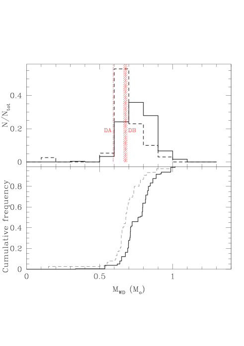
Figure 12: Top panel: Mass distributions of WDs orbiting mild and strong barium stars (dashed and solid lines, respectively) under the hypothesis of maximum concentration. The red shaded areas labeled DA and DB correspond to the average masses ($\pm 1\sigma$) for field WDs. Bottom panel: Cumulative mass distributions corresponding to the two samples from the top panel. The maximum vertical distance between the two curves is 0.45.

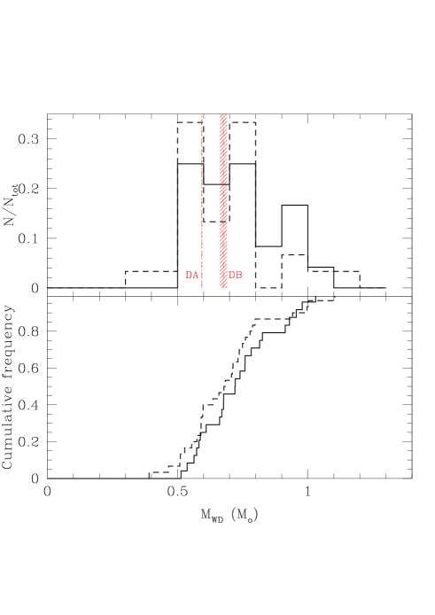
Figure 13: As in Fig. 12 but derived under the assumption of constant $Q$. In the bottom panel, the maximum difference between the two curves is 0.18.

Figure 14: Top panel: Relationships between the current barium-star mass ($M_{\rm Ba}$), the WD mass ($M_{\rm WD}$), and the WD-progenitor mass ($M_{\rm AGB,init}$). Mild and strong barium stars are represented by open and solid dots, respectively. Their differing sequences are caused by the adoption of two different values for $Q=M^{3}_{\rm WD}/(M_{\rm WD}+M_{\rm Ba})^{2}$. Bottom panel: Distribution of the ”initial” mass ratio $q^{\prime}=M_{\rm AGB,init}/M_{\rm Ba}$, which should in principle be larger than unity. Mild and strong barium stars are represented by dashed and solid lines, respectively.

Table 8: Abundances for s-process elements in barium stars, from various sources, as listed in the column Ref. The second column, labeled Ba, lists whether the star is considered as a mild (m) or strong (s) barium star. Assignment shifts (based on the abundances; see text) are indicated by an arrow. For completeness, the other columns list the component masses and orbital elements. Possibly inaccurate masses for the two stars with orbital periods close to 1 yr are listed in italics (see text).

HD/DM	Ba	$T_{\rm eff}$	$\log g$	$L_{\rm min}$	$L$	$L_{\rm max}$	$M_{\rm{Ba}}$	$M_{\rm WD}$	$P$	$e$	$f(M)$	[Fe/H]	[Y/Fe]	[Zr/Fe]	[La/Fe]	[Ce/Fe]	[hs/ls]	Ref
		(K)		(L⊙)			(M⊙)	(M⊙)	(d)		(M⊙)
$-64^{\circ}$4333	s	$4900\pm 100$	2.6	34	37	40	1.4$+0.1\atop-0.1$	0.61	386	0.03	0.068	-0.10	1.13	1.12	2.52	1.41	0.84	2
$-42^{\circ}$2048	s	$4400\pm 100$	1.6	170	234	303	1.9$+0.7\atop-0.5$	0.74	3260	0.08	0.065	-0.23	0.95	0.96	1.56	1.12	0.38	2
$-14^{\circ}$2678	m	$5200\pm 100$	$3.1\pm 0.2$	57	73	92	3.0$+0.2\atop-0.2$	0.80	3470	0.22	0.023	0.01	1.02	0.85	1.08	0.87	0.04	2
$-01^{\circ}$3022	m	$4832\pm 25$	$2.7\pm 0.4$	51	56	61	1.6$+0.1\atop-0.1$	0.55	3253	0.28	0.016	-0.14	0.58	0.71	0.44	0.33	-0.26	4
5424	s	$4728\pm 80$	$2.5\pm 0.0$	33	60	90	1.3$+0.4\atop-0.3$	0.59	1881	0.23	0.005	-0.43	1.30	1.05	1.82	1.67	0.57	1
16458	s	$4550\pm 25$	$1.8\pm 0.2$	205	217	229	1.9$+0.1\atop-0.1$	0.72	2018	0.1	0.041	-0.64	1.06	1.29	1.43	1.29	0.19	1
18182	m	$4858\pm 31$	$2.5\pm 0.4$	60	65	71	1.8$+0.2\atop-0.1$	0.59	8059	0.31	0.0002	-0.17	0.50	0.35	0.40	0.35	-0.05	2
20394	s	$4926\pm 17$	$2.5\pm 0.0$	578	69	82	2.0$+0.2\atop-0.2$	0.76	2226	0.2	0.002	-0.27	1.00	1.14	1.70	1.28	0.42	2
24035	s	$4700\pm 100$	$2.5\pm 0.2$	13	26	39	1.3$+0.3\atop-0.2$	0.57	377.8	0.3	0.047	-0.23	1.35	1.20	2.70	1.58	0.87	2
27271	m	$5022\pm 40$	$2.9\pm 0.5$	68	82	98	2.9$+0.2\atop-0.2$	0.79	1693	0.22	0.024	-0.07	0.77	0.79	0.67	0.62	-0.13	1
31487	s	$4960\pm 50$	$3.1\pm 0.2$	124	141	160	3.4$+0.2\atop-0.3$	1.03	1066	0.05	0.038	-0.04	1.23	1.11	1.53	1.46	0.32	1
40430	m	$4930\pm 29$	$2.4\pm 0.2$	74	84	95	2.3$+0.2\atop-0.2$	0.68	5609	0.22	0.0025	-0.34	0.76	0.58	0.91	0.89	0.23	2
43389	s	$4000\pm 50$	$2.0\pm 0.5$	196	260	330	1.8$+0.4\atop-0.3$	0.72	1689	0.08	0.043	-0.35	0.91	0.32	1.53	1.22	0.76	1
44896	s	$4300\pm 100$	0.7	526	676	841	3.0$+1.2\atop-1.0$	0.96	629	0.02	0.048	-0.25	1.16	0.81	0.93	0.87	-0.09	11
46407	s	$4854\pm 100$	$2.2\pm 0.4$	35	83	135	2.1$+0.6\atop-0.7$	0.78	457	0.013	0.035	-0.35	1.15	1.28	1.56	1.50	0.31	1
49641	s	$4400\pm 100$	$1.5\pm 0.2$	345	457	579	2.7$+1.2\atop-0.8$	0.91	1785	0.07	0.003	-0.3	0.89	0.53	1.86	1.04	0.74	2
49841	m	5200	3.2	49	61	74	2.8$+0.2\atop-0.2$	0.78	897	0.16	0.032	0.2	0.85	0.65	0.81	0.56	-0.06	9
50082	s	$4789\pm 100$	$2.4\pm 0.5$	60	63	66 2	1.6$+0.3\atop-0.2$	0.67	2896	0.19	0.027	-0.32	0.86	1.04	1.42	1.35	0.44	1
51959	m	$4814\pm 34$	$3.2\pm 0.2$	11	13	16	1.2$+0.1\atop-0.1$	0.47	9718	0.53	0.0005	-0.21	0.98	1.25	0.94	1.02	-0.13	4
53199	m	$5119\pm 28$	$2.9\pm 0.2$	47	55	64 1	2.5$+0.1\atop-0.1$	0.71	8314	0.24	0.028	-0.20	0.68	0.70	1.06	0.93	0.31	2
58121	m	$4600\pm 100$	$1.8\pm 0.2$	121	142	163	2.6$+0.5\atop-0.4$	0.73	1214	0.14	0.015	-0.01	0.41	0.26	0.50	0.36	0.10	2
58368	m	$5000\pm 100$	$2.6\pm 0.2$	37	43	49	2.6$+0.1\atop-0.2$	0.73	672	0.22	0.021	0.04	0.85	0.60	1.13	0.86	0.27	2
59852	m	$5000\pm 100$	$2.2\pm 0.2$	81	90	100	2.5$+0.2\atop-0.3$	0.71	3464	0.15	0.0022	-0.22	0.40	0.27	0.39	0.41	0.06	2
77247	m	$5050\pm 100$	$2.5\pm 0.5$	306	346	388	3.9$+0.1\atop-0.2$	0.94	80	0.09	0.005	-0.13	0.73	0.75	0.76	0.68	-0.02	4
84678	s	$4600\pm 100$	$1.7\pm 0.2$	154	189	227	2.3$+0.6\atop-0.5$	0.83	1630	0.06	0.062	-0.13	1.09	1.21	2.04	1.52	0.63	2
88562	s	$4000\pm 50$	$2.0\pm 0.5$	240	277	321	1.0$+0.1\atop-0.1$	0.51	1445	0.2	0.048	-0.53	0.93	0.43	1.15	1.02	0.41	1
91208	m	$5093\pm 67$	$2.9\pm 0.3$	35 9	39	43	2.3$+0.1\atop-0.2$	0.68	1754	0.17	0.022	-0.16	0.94	0.61	0.81	0.84	0.05	2
92626	s	$4800\pm 100$	2.3	171	214	259	3.1$+0.4\atop-0.6$	0.98	918	0.	0.042	-0.15	0.99	1.21	2.51	1.74	1.02	2
95193	m	$5008\pm 22$	$2.8\pm 0.1$	59	69	79	2.7$+0.1\atop-0.1$	0.76	1653	0.13	0.026	-0.04	0.75	0.26	0.50	0.36	-0.07	2
98839	m	$4917\pm 34$	$2.3\pm 0.6$	276	332	395	4.3$+0.2\atop-0.2$	1.00	16471	0.56	0.056	-0.05	0.10	0.17	0.35	0.30	0.19	4
101013	s	$4722\pm 32$	$2.3\pm 0.2$	77	108	141	1.7$+0.3\atop-0.3$	0.68	1711	0.2	0.037	-0.40	1.17	0.97	1.23	1.11	0.10	4
104979	m	$5100\pm 100$	$2.7\pm 0.2$	80	95	111	2.7$+0.1\atop-0.2$	0.75	19295	0.08	-	-0.26	0.71	0.85	1.11	1.06	0.31	6
107541	s	$5000\pm 100$	$3.2\pm 0.2$	8.9	11	14	1.1$+0.2\atop-0.1$	0.54	3570	0.1	0.029	-0.63	1.53	1.35	2.52	1.87	0.75	2
119185	m	$4919\pm 18$	$2.5\pm 0.0$	65	77	90.	1.7$+0.2\atop-0.2$	0.57	22065	0.6	-	-0.42	0.30	0.21	0.54	0.60	0.32	2
121447	s	$4000\pm 50$	$1.0\pm 0.5$	-	-	-	1.6$+0.1\atop-0.1$	0.6	185.7	0.015	0.025	-0.90	1.35	1.57	2.39	2.22	0.84	1

Table 8: Continued.

HD/DM	Ba	$T_{\rm eff}$	$\log g$	$L_{\rm min}$	$L$	$L_{\rm max}$	$M_{\rm{Ba}}$	$M_{\rm WD}$	$P$	$e$	$f(M)$	[Fe/H]	[Y/Fe]	[Zr/Fe]	[La/Fe]	[Ce/Fe]	[hs/ls]	Ref
		(K)		(L⊙)			(M⊙)	(M⊙)	(d)		(M⊙)
123949	s	$4378\pm 80$	$1.8\pm 0.5$	59	92	128	1.3$+0.3\atop-0.1$	0.58	8523	0.92	0.046	-0.23	0.91	0.88	1.21	1.28	0.35	1
134698	m	$4438\pm 30$	$1.7\pm 0.3$	163	192	225	1.5$+0.2\atop-0.2$	0.53	10005	0.95	0.054	-0.57	0.56	0.59	0.65	0.53	0.02	2
139195	m	$5029\pm 29$	$3.1\pm 0.2$	38	44	514	2.6$+0.1\atop-0.1$	0.74	5324	0.35	0.026	-0.07	0.72	0.79	0.62	0.54	-0.17	4
143899	m	$5144\pm 26$	$2.9\pm 0.3$	43	50	67	2.4$+0.1\atop-0.1$	0.71	1461	0.19	0.017	-0.29	0.86	0.57	0.90	0.90	0.19	2
154430	s	$4200\pm 100$	$1.2\pm 0.2$	382	685	1046	2.3$+1.4\atop-0.7$	0.81	1668	0.11	0.034	-0.36	0.93	0.97	2.00	1.33	0.71	2
178717	s	$3800\pm 50$	$1.0\pm 0.5$	156	1617	3189	1.6$+0.9\atop-0.7$	0.66	2866	0.43	0.006	-0.52	0.79	0.44	0.85	0.74	0.18	1
180622	m	$4600\pm 100$	$2.2\pm 0.2$	59	63	68	1.8$+0.3\atop-0.2$	0.59	4049	0.06	0.07	0.03	0.61	0.41	0.48	0.27	-0.13	2
183915	m$\rightarrow$s	$4494\pm 130$	$1.6\pm 0.4$	153	266	386	1.8$+1.0\atop-0.6$	0.60	4382	0.27	7E-05	-0.59	0.88	0.68	2.16	1.22	0.91	2
196673	m	$4914\pm 9$	$2.5\pm 0.3$	618	900	1206	5.0$+0.0\atop-0.1$	1.10	7780	0.59	0.020	0.12	0.00	0.25	0.39	0.31	0.23	4
199939	s	$4710\pm 9$	$2.4\pm 0.4$	159	214	271	2.8$+0.4\atop-0.4$	0.93	584.9	0.28	0.025	-0.22	1.38	1.19	1.72	1.67	0.41	1
200063	m	$4100\pm 100$	$1.1\pm 0.2$	206	753	1349	2.0$+1.3\atop-0.9$	0.64	1735	0.07	0.058	-0.34	0.88	0.62	1.33	0.93	0.38	2
201657	s	$4700\pm 100$	$2.2\pm 0.2$	63	80	100	1.8$+0.5\atop-0.4$	0.70	1710	0.17	0.004	-0.34	0.72	0.98	1.91	1.44	0.82	2
201824	s	$4937\pm 52$	$2.6\pm 0.2$	51	69	90	1.7$+0.4\atop-0.2$	0.68	2837	0.34	0.04	-0.40	0.91	0.87	1.58	1.48	0.64	2
202109	m	4700	2.4	120	147	176	3.4$+0.2\atop-0.4$	0.87	6489	0.22	0.023	-0.03	0.42	0.39	0.40	0.21	-0.10	9
204075	m	$5269\pm 53$	$1.7\pm 0.3$	418	561	741	4.5$+0.3\atop-0.2$	1.03	2378	0.28	0.004	-0.09	1.37	1.37	1.04	0.85	-0.43	5
205011	m	$4803\pm 21$	$2.5\pm 0.1$	59	73	88	1.8$+0.3\atop-0.3$	0.60	2837	0.24	0.034	-0.26	0.82	0.86	0.88	0.76	-0.02	4
210946	m	$4780\pm 76$	$2.4\pm 0.2$	50	74	99	1.8$+0.5\atop-0.4$	0.59	1529	0.13	0.041	-0.29	0.77	0.56	0.81	0.66	0.07	2
211594	s	$4947\pm 57$	$2.6\pm 0.1$	49	63	77	2.0$+0.3\atop-0.2$	0.76	1019	0.06	0.014	-0.29	1.20	1.18	2.31	1.57	0.75	2
218356	m	$4500\pm 100$	1.8	543	733	976	4.3$+0.2\atop-1.1$	1.00	111	0	4E-05	-0.06	0.45	0.26	0.90	0.51	0.35	7
223617	m	$4560\pm 20$	$2.2\pm 0.1$	61	65	70	1.4$+0.1\atop-0.1$	0.51	1294	0.06	0.0064	-0.20	0.70	0.73	1.03	0.67	0.14	4
NGC
2420-173	s$\rightarrow$m	$5150\pm 100$	2.2	95	128	173	3.0$+0.3\atop-0.4$	0.80	1479	0.43	0.008	-0.26	1.00	0.72	0.62	0.59	-0.26	10

References: (1) Karinkuzhi et al. (2018); (2) de Castro et al. (2016); (3) Allen & Barbuy (2006); (4) This work; (5) Merle et al. (2016); (6) Karinkuzhi & Goswami (2015); (7) Luck (2014) (8) Smith (1984); (9) Pereira et al. (2011); (10) Van der Swaelmen et al. (2017); (11) Smith (1984)

8 Mass distribution of the WD progenitor and initial mass ratio of the system

In this section, we derive the mass distribution of the WD progenitor (denoted $M_{\rm AGB,ini}$) and compare it with the mass of the barium star ($M_{\rm Ba}$), expecting that $q^{\prime}\equiv M_{\rm AGB,ini}/M_{\rm Ba}>1$, unless mass accretion by the barium star has substantially increased its current mass over its initial value. For the purpose of deriving $M_{\rm AGB,ini}$, we use the most recent full-range initial–final mass relationship (IFMR) as derived by El-Badry et al. (2018) from the Gaia DR2. The IFMR has been applied to the WD masses listed in Table 8 to get $M_{\rm AGB,ini}$. The resulting mass ratio $q^{\prime}$ is shown in the bottom panel of Fig. 14. This ”initial” $q^{\prime}$ distribution appears to be very different among mild and strong barium stars. As shown in the top panel of Fig. 14, this difference may ultimately be traced back to the difference between the $Q$ values characterizing mild and strong barium stars (Fig. 8). Nevertheless, this constitutes a clear difference among mild and strong barium stars, and one may wonder whether it could be the cause of their different levels of chemical pollution. This question is addressed in Sect. 9.

The procedure used here to derive $M_{\rm AGB,ini}$ assumes that the binary evolution did not affect the IFMR, but there is no guarantee that this statement is true, quite the contrary. Still, most of the barium systems displayed in the upper right panel of Fig. 14 have $q^{\prime}>1$ as expected, the only exceptions being the mild barium stars with the lowest masses (open circles falling below the $q^{\prime}=1$ line). Some of these have WDs with masses lower than 0.5 M_⊙, which is unphysical since this corresponds to progenitors which never reached the TP-AGB (see, e.g., Merle et al., 2016), and therefore could not trigger the s-process whose ashes are responsible for making the barium star.

Some of the WD companions to barium stars have large masses (with a few just above 1 M_⊙), pointing towards initial AGB masses larger than 5 M_⊙ (top panel of Fig. 14). It is worth noting that AGB stars of such large masses and with solar (or slightly subsolar) metallicities are not able to produce substantial s-process enrichments (see, e.g., Cristallo et al., 2015; Karakas & Lugaro, 2016; Cseh et al., 2018). For that reason, these WD masses above 1 M_⊙ derived under the assumption of constant $Q$ are likely somewhat overestimated; we note that the most-peaked WD distribution in Fig. 12 is in that respect preferable, as it contains just one WD with a mass just above 1 M_⊙. Except for those extreme cases however the WD mass distributions presented in Figs. 12 and 13 are compatible with current expectations from AGB s-process nucleosynthesis.

9 The period–mass–metallicity–abundance connection

In this section, we investigate the correlation between abundances, orbital periods, metallicities, and masses (barium star and WD companion). So far, the overabundances of s-process elements in barium stars were tested for possible correlation primarily with orbital periods (Jorissen & Boffin, 1992; Boffin & Zac̀s, 1994; Bonačić Marinović & Pols, 2004; Abate et al., 2015a; Karinkuzhi et al., 2018), and to a lesser extent with metallicity (Jorissen et al., 2016; Merle et al., 2016). Our current analysis (especially Sect. 7.2) advocates the addition of barium-star and WD masses to the analysis (see also Merle et al., 2016).

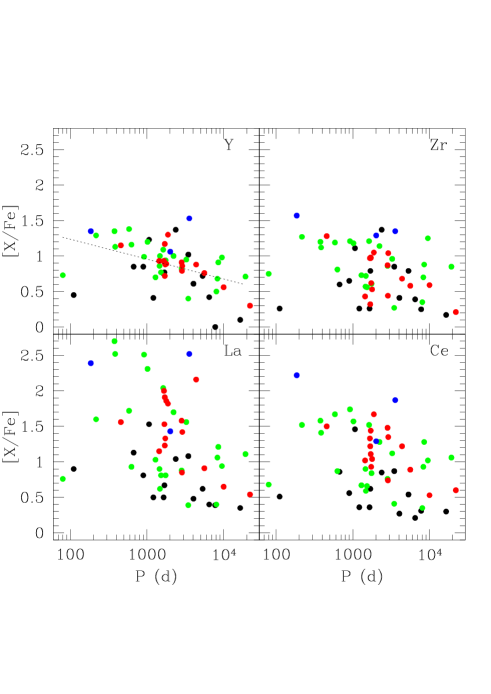
Figure 15: Period–abundances relationship for s-process elements Y, Zr, La, and Ce. In the panel corresponding to Y, the dotted line is a least-square fit to the data, illustrating the trend existing with orbital period. Blue ([Fe/H] $<-0.6$), red (from $-0.6$ to $-0.3$), green (from $-0.3$ to $-0.1$), and black ([Fe/H] $\geq-0.1$) symbols denote stars of increasing metallicities.

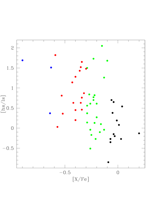
Figure 16: Efficiency of the s-process expressed as [hs/ls] $\equiv\mathrm{([La/Fe]+[Ce/Fe])}-\mathrm{([Y/Fe]+[Zr/Fe])}$ as a function of metallicity [Fe/H] and color-coded as in Fig. 15.

Figure 17: Barium-star mass vs. [Fe/H], color-coded as in Fig. 15.

Abundances for the barium stars were derived as described in Karinkuzhi et al. (2018), and are listed in Table 8; they are also displayed in Fig. 15 as a function of the orbital period. Earlier studies (as listed above) claimed the presence of a general trend of decreasing s-process overabundance with increasing orbital period. In our data sample, this trend is visible only for Y. For Zr, La, and Ce, the trend, if any, is blurred by a large scatter. As shown by the color sequence in Fig. 15 (black – green – red – blue, corresponding to stars of decreasing metallicities; see caption of Fig. 15), this scatter is partly due to metallicity, since high-metallicity stars (black points) appear mostly at the bottom of the cloud, whereas low-metallicity stars (blue points) appear mostly at its top. The role of metallicity is best revealed by Fig. 16, which displays the s-process efficiency expressed as [hs/ls] $\equiv\mathrm{([La/Fe]+[Ce/Fe])}-\mathrm{([Y/Fe]+[Zr/Fe])}$ as a function of metallicity. The trend seen on that plot is not surprising given that the efficiency of the s-process nucleosynthesis, when controlled by the ¹³C($\alpha$,n)¹⁶O neutron source, has been shown to increase with decreasing metallicity (e.g., Clayton, 1988; Cseh et al., 2018, and references therein).

The barium-star mass will play a role as well, since (i) barium-star mass and metallicity vary together (lower masses corresponding to lower metallicities, as expected; see Fig. 17), and (ii) larger barium-star masses imply larger envelope masses, and therefore higher dilution of the accreted matter in the envelope (at least as long as the envelope is convective, notwithstanding any influence of a possible thermohaline mixing erasing the influence of the envelope mass; e.g., Husti et al., 2009).

To summarize the findings of this and previous sections, Table 9 shows the Pearson’s correlation-coefficient matrix of the variables discussed so far, and they reveal in a quantitative way most of the results discussed so far:

• (i) $M_{\rm Ba}$ and $M_{\rm WD}$ are the most strongly correlated variables by construction, since $M_{\rm WD}$ has been derived from $M_{\rm Ba}$ under the assumption of constant $Q\equiv M_{\rm WD}^{3}/(M_{\rm Ba}+M_{\rm WD})^{2}$ separately for mild and strong barium stars.

• (ii) The strong correlation between $e$ and $P$ is the manifestation of the so-called ‘$e-P$ diagram’.

• (iii) $M_{\rm Ba}$ and [Fe/H] are well correlated (Fig. 17).

• (iv) S-process abundances are well correlated with each other, and moderately anti-correlated with $P$ (the anti-correlation with $P$ is the largest for [Y/Fe] and [La/Fe]; Fig. 15). However, the strongest correlation between dynamical and chemical parameters is between $q^{\prime}$ and [La/Fe], [Ce/Fe], as anticipated in Sect. 8.

The discussion of the implications of these results on the formation scenario of barium stars (and in particular the origin of the mild/strong nature of the barium star) is deferred to a forthcoming paper.

Table 9: Lower left half of the (symmetric) Pearson’s correlation-coefficient matrix of the variables $M_{\rm Ba}$, $M_{\rm WD}$, $q^{\prime}$, $P$, $e$, $f(M_{\rm Ba},M_{\rm WD})$, [Fe/H], [Y/Fe], [Zr/Fe], [La/Fe], [Ce/Fe]. (Nondiagonal) Correlation coefficients larger than 0.4 (in absolute value) are in boldface. This value of the correlation coefficient corresponds to a two-tailed $p$-value of 0.17%, meaning that an uncorrelated system will produce datasets that have a Pearson’s correlation coefficient at least as extreme as $\pm 0.4$ for 0.17% of the draws. For a correlation coefficient of 0.3, the two-tailed $p$-value rises to 2%.

	$M_{\rm Ba}$	$M_{\rm WD}$	$q^{\prime}$	$P$	$e$	$f(M_{\rm Ba},M_{\rm WD})$	[Fe/H]	[Y/Fe]	[Zr/Fe]	[La/Fe]	[Ce/Fe]
$M_{\rm Ba}$	1.
$M_{\rm WD}$	0.913	1.
$q^{\prime}$	0.165	0.532	1.
$P$	-0.058	-0.174	-0.284	1.
$e$	-0.025	-0.162	-0.304	0.593	1.
$f(M_{\rm Ba},M_{\rm WD})$	-0.207	-0.086	0.154	-0.126	-0.079	1.
[Fe/H]	0.583	0.471	-0.078	0.001	-0.031	0.032	1.
[Y/Fe]	-0.364	-0.132	0.351	-0.462	-0.360	0.202	-0.373	1.
[Zr/Fe]	-0.285	-0.078	0.309	-0.330	-0.251	0.164	-0.331	0.827	1.
[La/Fe]	-0.363	-0.089	0.489	-0.390	-0.370	0.212	-0.432	0.718	0.715	1.
[Ce/Fe]	-0.406	-0.121	0.498	-0.357	-0.297	0.186	-0.539	0.794	0.811	0.913	1.

10 Conclusion

This study completes the radial-velocity monitoring of samples of mild and strong barium stars, and extrinsic S stars initiated in 1984 with the CORAVEL spectrograph. All stars monitored (37 strong barium stars, 40 mild barium stars, and 34 extrinsic S stars) turn out to be binaries (except for the mild barium star HD 95345), and provide a first-hand collection of 111 post-mass-transfer systems among which 105 with orbital elements will serve in the future as benchmark systems for binary-evolution models.

Our HERMES/Mercator radial-velocity monitoring delivered the long-period orbits not yet available in the mid-course analysis published in 1998 (Jorissen et al., 1998). We found several orbits with periods in the range $1-4\times 10^{4}$ d ($\sim 110$ yr). With the present study, we clearly show that the wind-accretion scenario invoked to account for the s-process pollution in the widest systems (Boffin & Jorissen, 1988; Abate et al., 2015b, 2018) is no longer efficient in systems with periods in excess of $4\times 10^{4}$ d due to the low accretion cross-section of the wind in such systems.

The eccentricity–period diagram further reveals that, on average, barium stars with strong s-process overabundances are restricted to the period range 200 – 5000 d (with two exceptions at $10^{4}$ d), whereas mild barium stars are found in the range 700 – 20000 d (with two exceptions at $\sim 100$ d). The avoidance region ($P>10^{3}$ d, $e<0.07$) is confirmed, and is likely a vestige of a similar avoidance region (albeit extending towards larger eccentricities) in pre-main sequence binaries. Almost all barium systems with periods shorter than $10^{3}$ d are circular, and this property is likely attributable to the circularisation occurring as the giant star ascends the red giant branch (RGB), as demonstrated by the models of Escorza et al. (2019). Extrinsic S stars, which are still ascending the RGB confirm this statement since S systems with $P<10^{3}$ d are not necessarily circular, and this is the only property that they do not share with barium systems.

Thanks to Gaia DR2 parallaxes and spectral-energy distribution fits, our barium-star sample could be located in the Hertzsprung-Russell diagram, and the position of individual stars compared with STAREVOL tracks of the corresponding metallicity (Siess et al., 2000; Siess & Arnould, 2008). Metallicities for the barium stars were either collected from the literature when available or were derived from Mercator/HERMES high-resolution spectra. This comparison then gives access to the barium-star masses ($M_{\rm Ba}$), which in turn yield the companion masses ($M_{\rm WD}$) under the assumption of a constant $Q=M_{\rm WD}^{3}/(M_{\rm Ba}+M_{\rm WD})^{2}$ value (different for mild and strong barium stars). This constancy was envisioned by Webbink (1988) and McClure & Woodsworth (1990) and is clearly confirmed by our present extensive samples. The cause of that property, which has not been clearly identified, merits a specific discussion; this is deferred to a forthcoming paper.

The companion masses appear to be restricted in the range 0.5 – 1.1 M_⊙, as expected for WDs. The peak of the distribution lies around 0.55 – 0.70 M_⊙, exactly as for field DA and DB WDs. The heaviest WDs around barium stars point at AGB-progenitor masses around 5 M_⊙, at the edge of the predictions for efficient s-process AGB nucleosynthesis.

In the hope of disentangling the various parameters involved in fixing the s-process overabundance levels in barium stars (orbital separation, dilution factor in the barium-star envelope, final AGB core mass, metallicity etc.), we performed a correlation analysis involving parameters $M_{1},M_{2},q^{\prime},P,e,f(M_{1},M_{2})$, [Fe/H], [Y/Fe], [Zr/Fe], [La/Ce], and [Ce/Fe]. Significant correlations or anti-correlations (with coefficients in excess of 0.4) were found between $P$ and $e$, and between s-process abundances, $P$, $q^{\prime}$, and metallicity (as expected). More unexpected is the strong correlation observed between $M_{\rm Ba}$ and metallicity. Such a correlation must be a consequence of the age–metallicity relationship, which predicts that giants of low metallicities ([Fe/H] $\leq-0.4$) in the solar neighborhood must be older than about 5 Gyr (e.g., Fig. 3 of Feuillet et al., 2018), and must therefore be of low mass ($\la 1.3$ M_⊙). A strong correlation is also found between [La/Fe], [Ce/Fe], and the “initial” mass ratio $q^{\prime}$. This is the strongest link found so far between dynamical and chemical abundances; it dominates over any effect related to the orbital period. This is clearly the root of the difference between mild and strong barium stars, which is visible as well in their different current $Q$ values, implying that strong barium stars originate from systems with a mass ratio above $\sim 1.5$. This is the combined result of the masses of strong barium stars being on average smaller than those of mild barium stars, and of the tendency for WDs around strong barium stars to be more massive on average. The first effect contributes to reducing the dilution factor of the accreted matter in the barium-star envelope. This finding will certainly turn out to be a key constraint for the evolutionary models of binary stars aiming at reproducing the properties of barium stars. Initial conditions adopted in these models should certainly conform to our key finding that the initial mass-ratio $q^{\prime}$ is very far from being uniform, and differs for strong and mild barium stars.

Appendix A Spectroscopic binaries with no orbital solutions yet

This section presents velocity curves for the spectroscopic binaries for which orbital solutions are yet to be obtained, namely the extrinsic S star BD -21^∘2601 (Fig. 18), and the mild barium stars HD 50843, HD 65854, and HD 95345 (Figs. 19, 20, and 21). In the figures of this section and the following, all data points posterior to JD 2454900 were obtained with the HERMES spectrograph while the previous ones are all from CORAVEL, the latter being moreover characterized by larger error bars ($\sim 0.3$ km s^-1).

Figure 18: Top panel: Radial velocities for the S star BD -21^∘2601. Older data are from CORAVEL, newer from HERMES. No zero-point offset has been applied to the CORAVEL data. Bottom panel: Same as top, but for HERMES velocities only.

Figure 19: Same as Fig. 18 but for the mild barium star HD 50843. No offset has been applied to the CORAVEL data.

Figure 20: Same as Fig. 18 but for the mild barium star HD 65854. No zero-point offset has been applied to the CORAVEL data.

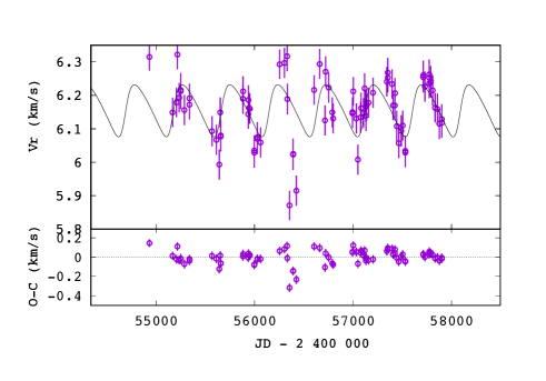
Figure 21: Top panel: Same as Fig. 18 but for the mild barium star HD 95345. A zero-point offset of +0.6 km s^-1 has been applied to the CORAVEL data. Bottom panel: Tentative orbit based on HERMES data only (see also Table 4).

Appendix B Orbital solutions

This Appendix presents all orbital solutions superimposed on the velocity data.

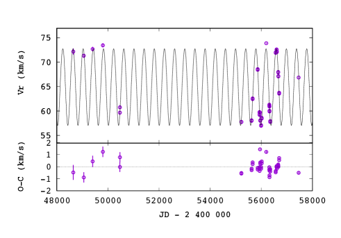
Figure 43: Upper panel: Radial velocities of the S star CD -28^∘3719 (= Hen 4-18) and the associated orbit. Older data are from CORAVEL, newer from HERMES. Lower panel: O-C residuals.

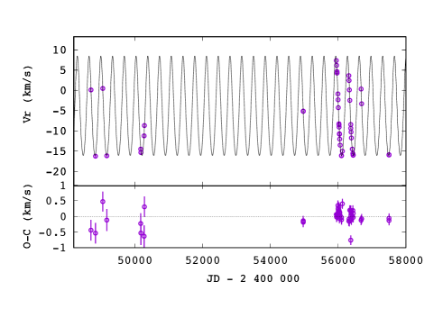
Figure 44: Upper panel: Radial velocities of the S star CD -25^∘10393 (= Hen 4-147) and the associated orbit. Older data are from CORAVEL, newer from HERMES. Lower panel: O-C residuals.

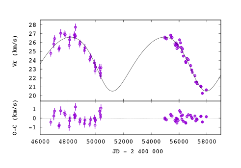
Figure 45: Upper panel: Radial velocities of the S star BD $+31^{\circ}$4391 and the associated orbit. Older data are from CORAVEL, newer from HERMES. Lower panel: O-C residuals.

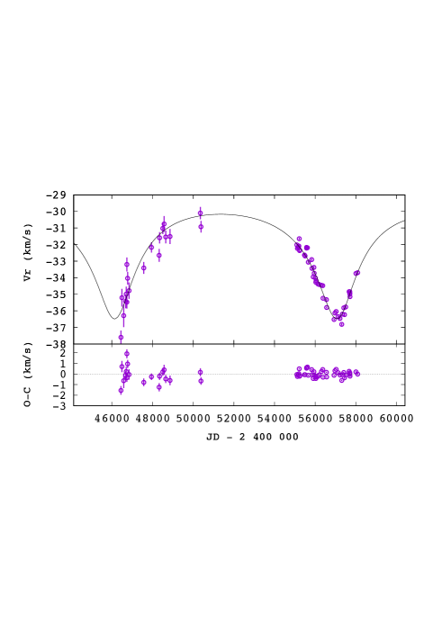
Figure 46: Upper panel: Radial velocities of the S star BD +79^∘156 and the associated orbit. Older data are from CORAVEL, newer from HERMES. Lower panel: O-C residuals.

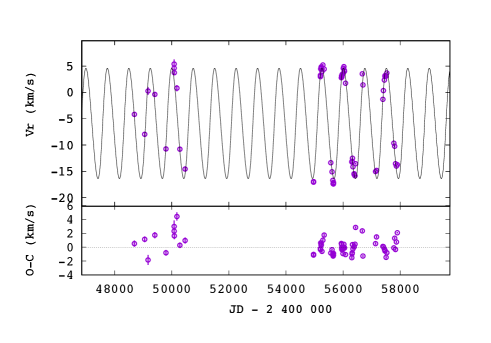
Figure 47: Upper panel: Radial velocities of the S star V420 Hya and the associated orbit. Older data are from CORAVEL, newer from HERMES. Lower panel: O-C residuals.

Appendix C Fe line list

Table 10 presents the Fe lines used to derive the metallicities of barium stars.

Table 10: The Fe lines used to derive the metallicities of barium stars, along with their excitation potential and oscillator strength.

$\lambda$	$\chi_{\rm low}$	$\log gf$
(Å)	(eV)
5217.919	3.640	-1.719	Fe I
5223.183	3.635	-1.783	Fe I
5231.395	3.573	-2.951	Fe I
5232.940	2.940	-0.076	Fe I
5236.202	4.186	-1.497	Fe I
5243.776	4.256	-1.050	Fe I
5272.268	5.033	-1.038	Fe I
5285.127	4.434	-1.540	Fe I
5302.300	3.283	-0.720	Fe I
5321.108	4.434	-1.089	Fe I
5322.041	2.279	-2.802	Fe I
5324.179	3.211	-0.103	Fe I
5326.142	3.573	-2.071	Fe I
5339.929	3.266	-0.684	Fe I
5364.871	4.445	0.228	Fe I
5365.399	3.573	-1.020	Fe I
5379.574	3.694	-1.514	Fe I
5398.279	4.445	-0.630	Fe I
5405.775	0.990	-1.858	Fe I
5406.775	4.371	-1.620	Fe I
5410.910	4.473	0.339	Fe I
5412.784	4.434	-1.716	Fe I
5417.033	4.415	-1.580	Fe I
5434.524	1.011	-2.119	Fe I
5436.295	4.386	-1.440	Fe I
5445.042	4.386	-0.020	Fe I
5501.465	0.958	-3.046	Fe I
5506.779	0.990	-2.793	Fe I
5567.391	2.608	-2.617	Fe I
5568.810	3.635	-2.850	Fe I
5569.618	3.417	-0.486	Fe I
5572.842	3.396	-0.275	Fe I
5573.102	4.191	-1.317	Fe I
5576.089	3.430	-0.900	Fe I
5586.756	3.368	-0.120	Fe I
5587.574	4.143	-1.750	Fe I
5811.914	4.143	-2.330	Fe I
5852.219	4.548	-1.230	Fe I
5853.148	1.485	-5.180	Fe I
5853.683	4.191	-2.590	Fe I
5855.076	4.608	-1.478	Fe I
5856.088	4.294	-1.327	Fe I
5857.802	5.033	-1.767	Fe I
5858.778	4.220	-2.160	Fe I
5859.586	4.549	-0.419	Fe I
5927.789	4.652	-0.990	Fe I
5929.677	4.548	-1.310	Fe I
5930.180	4.652	-0.230	Fe I
5934.655	3.928	-1.070	Fe I
5958.333	2.176	-4.160	Fe I
5425.257	3.199	-3.220	Fe II
5432.967	3.267	-3.527	Fe II
5534.847	3.245	-2.865	Fe II
5991.376	3.153	-3.647	Fe II
6238.392	3.889	-2.600	Fe II
6247.557	3.892	-2.435	Fe II
6416.919	3.892	-2.877	Fe II
6432.680	2.891	-3.570	Fe II
6456.383	3.903	-2.185	Fe II