Abstract

The LHC Higgs data is showing a gradual inclination towards the SM result and realization of an SM-like limit becomes essential for BSM scenarios to survive. Considering the accuracy that can be achieved in future colliders, BSMs that acquire the alignment limit with an SM-like Higgs boson can surpass others in the long run. Using a convenient parametrization, we demonstrate that the alignment limit for CP-conserving 3HDMs takes on the same analytic structure as that in the case of 2HDMs. Using the example of a $Z_{3}$-symmetric 3HDM, we illustrate how such alignment conditions can be efficiently implemented for numerical analysis in a realistic scenario.

1 Introduction

In the post Higgs discovery era, the absence of any direct sign of new physics (NP) at the LHC has already pushed many beyond the Standard Model (BSM) scenarios at bay. An alternative way to find hints for NP will be to look for deviations of Higgs couplings from their corresponding Standard Model (SM) predictions. However, since the discovery of the Higgs boson, the LHC Higgs data has been gradually drifting towards the SM expectations. In fact, deviations in the observed Higgs signal strengths from their respective SM values seem to have been significantly reduced with the increased sensitivity at the LHC Run II [1, 2]. But it is still possible for BSM scenarios to be hiding behind the curtain, camouflaging themselves with an SM-like Higgs. Thus, in anticipation that the LHC Higgs data will continue to incline towards the SM expectations with increasing accuracy, those BSM scenarios which can deliver an SM-like Higgs in a certain alignment limit will have an upper hand in the future survival race. In this paper, we uphold the three Higgs-doublet models (3HDMs) as potential candidates for such BSM scenarios.

Adding replicas of the SM Higgs-doublet constitutes one of the simplest ways to extend the SM for such extensions do not alter the tree-level value of the electroweak (EW) $\rho$-parameter. A lot of attention has already been given to the two Higgs-doublet models (2HDMs)[3, 4] where the scalar sector of the SM is extended by an additional Higgs-doublet. As a next step, recent years have seen a growing interest in the topic of 3HDMs[5, 6, 7, 8, 9, 10, 11, 12, 13, 14, 15, 16, 17, 18, 19, 20, 21, 22, 23, 24, 25, 26, 27, 28] where two additional Higgs-doublets are added to the SM scalar sector. Therefore, 3HDMs conform to the aesthetic appeal of having three generations of scalars on equal footing to three fermionic generations in the SM[29]. In such models, the $125$ GeV scalar observed at the LHC is only the first to appear in a series of many others to follow. Evidently, the rich scalar spectrum of the 3HDM must contain one physical scalar having properties similar to those of the SM Higgs boson, which can serve as a competent candidate for the $125$ GeV scalar. The limit in which the lightest CP-even scalar possesses SM-like tree-level couplings with the fermions and the vector bosons is usually dubbed as the alignment limit. In the case of 2HDMs, the analytic condition for alignment is well known[30, 31, 32] and it has been very useful in analyzing 2HDMs in the light of the Higgs data[33, 34, 35, 36, 37, 38, 39, 40, 41, 42]. However, in the case of multi Higgs-doublet models with more than two Higgs-doublets, although the general recipe for obtaining alignment has been studied earlier in the literature[17, 43, 24], analytic expressions suitable for practical use are currently lacking. In this paper, we attempt to find the conditions for alignment in 3HDMs, in a simple form that can be easily implemented in practical models to investigate several aspects of 3HDMs. In fact, using a convenient parametrization for CP conserving 3HDMs, we will demonstrate that the requirement of an SM-like Higgs results in simple equations which resemble very much to the alignment condition in CP conserving 2HDMs.

Our paper will be organized as follows. In Sec. 2 we will briefly revisit the general prescription for obtaining an SM-like Higgs in multi Higgs-doublet models. Then we will use this to recover the alignment limit in 2HDMs, and extend the idea to the case of 3HDMs. In Sec. 3 we will illustrate how our results of Sec. 2 can substantially simplify the analysis of a CP conserving 3HDM. Finally, our findings will be summarized in Sec. 4.

2 The alignment limit

As mentioned earlier, the alignment limit is defined as the set of conditions under which the lightest CP-even scalar mimics the SM Higgs by possessing SM-like gauge and Yukawa couplings at the tree-level. To illustrate how such a limit can be reached in a multi Higgs-doublet scenario, let us consider a general $n$ Higgs-doublet model ($n$HDM) where the $k$-th doublet is expanded in terms of its component fields as follows:

$$\phi_{k}=\begin{pmatrix}w_{k}^{+}\\ (h_{k}+iz_{k})/\sqrt{2}\end{pmatrix}\,,\qquad(k=1,2,\dots,n)\,.$$ (1)

Under the assumption that all the parameters in the $n$HDM scalar potential are real, there will be no mass mixing between the $h_{k}$ and the $z_{k}$ fields. Denoting by $\left\langle\phi_{k}\right\rangle=v_{k}/\sqrt{2}$ the vacuum expectation value (VEV) for $\phi_{k}$ after spontaneous symmetry breaking (SSB), the total EW VEV, $v$, can be identified as

$$v^{2}=\sum_{k=1}^{n}v_{k}^{2}=(246\,\,{\rm GeV})^{2}\,.$$ (2)

To gain some intuitive insights into the alignment limit of an $n$HDM, it is instructive to take a closer look at the scalar kinetic Lagrangian which contains the following trilinear couplings:

$${\mathscr{L}}_{\rm kin}^{S}=\sum_{k=1}^{n}|D_{\mu}\phi_{k}|^{2}\ni\frac{g^{2}}{2}W_{\mu}^{+}W^{\mu-}\left(\sum_{k=1}^{n}v_{k}h_{k}\right)\equiv\frac{g^{2}v}{2}W_{\mu}^{+}W^{\mu-}\left(\frac{1}{v}\sum_{k=1}^{n}v_{k}h_{k}\right)\,,$$ (3)

where $g$ stands for the $SU(2)_{L}$ gauge coupling. Clearly, the combination,

$$H_{0}=\frac{1}{v}\sum_{k=1}^{n}v_{k}h_{k}\,,$$ (4)

will resemble to the SM Higgs boson in its tree-level gauge couplings. It is also not very difficult to show that $H_{0}$ will have SM-like Yukawa couplings too[17]. However, this state $H_{0}$, in general, is not guaranteed to be a physical eigenstate. Therefore, the alignment limit will emerge as the limit when $H_{0}$ aligns itself completely with the lightest CP-even physical scalar ($h$) in the spectrum.

2.1 Alignment in 2HDM

To begin with let us apply the result of the previous section to retrieve the alignment limit in the 2HDM case. Following the definition in Eq. (4), the state $H_{0}$ and its orthogonal combination, $R$, can be obtained by the following orthogonal rotation:

$$\begin{pmatrix}H_{0}\\ R\end{pmatrix}={\cal O}_{\beta}\begin{pmatrix}h_{1}\\ h_{2}\end{pmatrix}=\begin{pmatrix}\cos\beta&\sin\beta\\ -\sin\beta&\cos\beta\end{pmatrix}\begin{pmatrix}h_{1}\\ h_{2}\end{pmatrix}\,,$$ (5)

where $\tan\beta=v_{2}/v_{1}$. On the other hand, the physical mass eigenstates, $h$ and $H$, are extracted using another orthogonal rotation characterized by the angle, $\alpha$, as follows:

$$\begin{pmatrix}h\\ H\end{pmatrix}={\cal O}_{\alpha}\begin{pmatrix}h_{1}\\ h_{2}\end{pmatrix}=\begin{pmatrix}\cos\alpha&\sin\alpha\\ -\sin\alpha&\cos\alpha\end{pmatrix}\begin{pmatrix}h_{1}\\ h_{2}\end{pmatrix}\,.$$ (6)

Inverting Eq. (5) and then plugging it on the right hand side of Eq. (6), we can write

$$\begin{pmatrix}h\\ H\end{pmatrix}={\cal O}_{\alpha}{\cal O}_{\beta}^{T}\begin{pmatrix}H_{0}\\ R\end{pmatrix}=\begin{pmatrix}\cos(\alpha-\beta)&\sin(\alpha-\beta)\\ -\sin(\alpha-\beta)&\cos(\alpha-\beta)\end{pmatrix}\begin{pmatrix}H_{0}\\ R\end{pmatrix}\,.$$ (7)

Thus, $h$ will completely overlap with $H_{0}$ if

$$\cos(\alpha-\beta)=1 \Rightarrow \alpha=\beta\,,$$ (8)

which defines the alignment limit in 2HDMs.

2.2 Alignment in 3HDM

In the case of 3HDMs let us first parametrize the VEVs as follows:

$$v_{1}=v\cos\beta_{1}\cos\beta_{2}\,,\qquad v_{2}=v\sin\beta_{1}\cos\beta_{2}\,,\qquad v_{3}=v\sin\beta_{2}\,.$$ (9)

Thus, the analogue of Eq. (5) for 3HDM will read

$$\begin{pmatrix}H_{0}\\ R_{1}\\ R_{2}\end{pmatrix}={\cal O}_{\beta}\begin{pmatrix}h_{1}\\ h_{2}\\ h_{3}\end{pmatrix}=\begin{pmatrix}\cos\beta_{2}\cos\beta_{1}&\cos\beta_{2}\sin\beta_{1}&\sin\beta_{2}\\ -\sin\beta_{1}&\cos\beta_{1}&0\\ -\cos\beta_{1}\sin\beta_{2}&-\sin\beta_{1}\sin\beta_{2}&\cos\beta_{2}\end{pmatrix}\begin{pmatrix}h_{1}\\ h_{2}\\ h_{3}\end{pmatrix}\,.$$ (10)

Note that the first row of ${\cal O}_{\beta}$ in the above equation is motivated from Eq. (4) but the choices for the second and the third rows are not unique. Our analysis does not depend on these choices. Next, in analogy with Eq. (6), ${\cal O}_{\alpha}$ will now be a $3\times 3$ orthogonal matrix which takes us to the physical basis, $(h\,H_{1}\,H_{2})^{T}$. Therefore, we can decompose ${\cal O}_{\alpha}$ as follows:

$${\cal O}_{\alpha} = {\cal R}_{3}\cdot{\cal R}_{2}\cdot{\cal R}_{1}\,,$$ (11a)

where,

$${\cal R}_{1}=\left(\begin{array}[]{ccc}\cos\alpha_{1}&\sin\alpha_{1}&0\\ -\sin\alpha_{1}&\cos\alpha_{1}&0\\ 0&0&1\\ \end{array}\right)\,,\quad{\cal R}_{2}=\left(\begin{array}[]{ccc}\cos\alpha_{2}&0&\sin\alpha_{2}\\ 0&1&0\\ -\sin\alpha_{2}&0&\cos\alpha_{2}\\ \end{array}\right)\,,\quad{\cal R}_{3}=\left(\begin{array}[]{ccc}1&0&0\\ 0&\cos\alpha_{3}&\sin\alpha_{3}\\ 0&-\sin\alpha_{3}&\cos\alpha_{3}\\ \end{array}\right)\,.$$ (11k)

Now, similar to Eq. (7), we can write

$$\left(\begin{array}[]{c}h\\ H_{1}\\ H_{2}\\ \end{array}\right) = {\cal O}_{\alpha}\cdot{\cal O}_{\beta}^{T}\left(\begin{array}[]{c}H^{0}\\ R_{1}\\ R_{2}\\ \end{array}\right)$$ (18)

in case of 3HDMs. For the convenience of notations in our analysis of 3HDMs, we introduce the matrix

$${\cal O}\equiv{\cal O}_{\alpha}\cdot{\cal O}_{\beta}^{T}\,,$$ (19)

where ${\cal O}_{\beta}$ and ${\cal O}_{\alpha}$ have been defined in Eqs. (10) and (11) respectively. Thus, for $h$ to overlap completely with $H_{0}$, we must require

$${\cal O}_{11}=1\,,$$ (20)

which can be expressed as

$$\cos\alpha_{2}\cos\beta_{2}\cos(\alpha_{1}-\beta_{1})+\sin\alpha_{2}\sin\beta_{2}=1\,.$$ (21)

After some simple trigonometric manipulations the above condition can be recast in the following form:

$$\left[\sin\left(\frac{\alpha_{1}-\beta_{1}}{2}\right)\cos\left(\frac{\alpha_{2}+\beta_{2}}{2}\right)\right]^{2}+\left[\cos\left(\frac{\alpha_{1}-\beta_{1}}{2}\right)\sin\left(\frac{\alpha_{2}-\beta_{2}}{2}\right)\right]^{2}=0\,,$$ (22)

which implies

$$\sin\left(\frac{\alpha_{1}-\beta_{1}}{2}\right)\cos\left(\frac{\alpha_{2}+\beta_{2}}{2}\right)=0\,,$$ (23a)

$${\rm and,} \cos\left(\frac{\alpha_{1}-\beta_{1}}{2}\right)\sin\left(\frac{\alpha_{2}-\beta_{2}}{2}\right)=0\,.$$ (23b)

These conditions together define the alignment limit for a CP-conserving 3HDM. One can easily check that the conditions of Eq. (23) admit the following two possibilities:

$$\alpha_{1}=\beta_{1}\,; \alpha_{2}=\beta_{2}\,,$$ (24)

$${\rm or,}\qquad\alpha_{1}=\pi+\beta_{1}\,; \alpha_{2}=\pi-\beta_{2}\,.$$ (25)

But, using Eq. (19) it can be verified that choosing condition (25) instead of condition (24) only amounts to redefinitions of the physical fields $H_{1}$ and $H_{2}$ as

$$H_{1}\to-H_{1}\,, {\rm and} H_{2}\to-H_{2}\,,$$ (26)

which are physically equivalent. Therefore, we choose condition (24) as the definition of alignment limit in 3HDMs, which, when compared with Eq. (7), looks very similar to the 2HDM case.

In passing, we note that Eq. (21) can be trivially satisfied in the limit $\sin\alpha_{2}\approx\sin\beta_{2}\approx 1$ which, in view of Eq. (9), corresponds to the situation where $\phi_{3}$ acquires the entire EW VEV and consequently $\phi_{1}$ and $\phi_{2}$ are rendered (almost) inert. However, barring such extreme VEV hierarchies, Eq. (24) must be obeyed so that an SM-like Higgs may emerge from the 3HDM scalar spectrum.

3 An example: 3HDM with $Z_{3}$ symmetry

At this point, it is reasonable to ask how close we need to be to the alignment limit in view of the current Higgs data. To analyze this, we proceed by defining the Higgs coupling modifiers as

$$\kappa_{x}=\frac{g_{hxx}}{(g_{hxx})^{\rm SM}}\,,$$ (27)

where $x$ stands for the massive fermions and vector bosons. Keeping in mind that among $H_{0}$, $R_{1}$ and $R_{2}$ in Eq. (18), only $H_{0}$ possesses trilinear coupling of the form $H_{0}VV$ ($V=W,Z$), we conclude

$$\kappa_{V}\equiv{\cal O}_{11}=\cos\alpha_{2}\cos\beta_{2}\cos(\alpha_{1}-\beta_{1})+\sin\alpha_{2}\sin\beta_{2}\,.$$ (28)

To obtain the fermionic coupling modifiers we need to know how the Higgs-doublets couple to the fermions. For this, we consider the example of a $Z_{3}$ symmetric 3HDM, in which the scalar doublets $\phi_{1}$ and $\phi_{2}$ transform nontrivially as follows:

$$\phi_{1}\to\omega\,\phi_{1}\,,\qquad\phi_{2}\to\omega^{2}\phi_{2}\,,$$ (29)

where $\omega=e^{2\pi i/3}$. Furthermore, some of the right handed fermionic fields transform under $Z_{3}$ as follows:

$$d_{R}\to\omega\,d_{R}\,,\qquad\ell_{R}\to\omega^{2}\ell_{R}\,,$$ (30)

where $d_{R}$ and $\ell_{R}$ denote the right handed down type quarks and charged leptons respectively. The rest of the fields in the theory are assumed to remain unaffected under $Z_{3}$. With these charge assignments, $\phi_{3}$ and $\phi_{2}$ will be responsible for masses of the up and down type quarks respectively, whereas $\phi_{1}$ will give masses to the charged leptons. Consequently, the fermionic coupling modifiers will be given by

$$\kappa_{u} = \frac{\sin\alpha_{2}}{\sin\beta_{2}}\,,$$ (31a)

$$\kappa_{d} = \frac{\sin\alpha_{1}\cos\alpha_{2}}{\sin\beta_{1}\cos\beta_{2}}\,,$$ (31b)

$$\kappa_{\ell} = \frac{\cos\alpha_{1}\cos\alpha_{2}}{\cos\beta_{1}\cos\beta_{2}}\,,$$ (31c)

all of which, as expected, approaches unity in the alignment limit defined by Eq. (24).

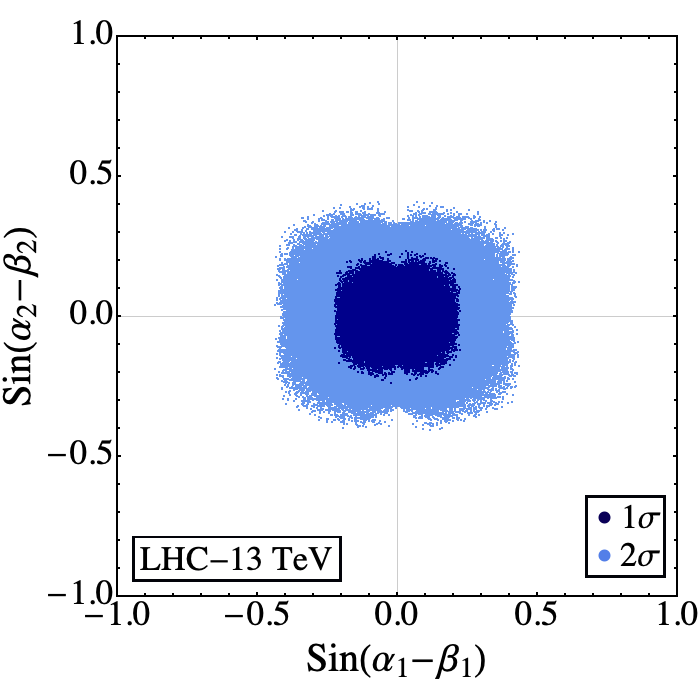
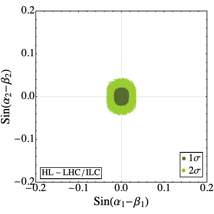
Figure 1: Allowed region in the $\sin(\alpha_{1}-\beta_{1})$-$\sin(\alpha_{2}-\beta_{2})$ plane from the current (left panel) [2] and the future (right panel) [44] measurements of $\kappa_{x}$. The darker and lighter shades represent $1\sigma$ and $2\sigma$ allowed regions respectively. While extracting bound using the projected accuracies at the HL-LHC and the ILC, the central values for all the $\kappa_{x}$ are assumed to be unity, i.e., consistent with the SM.

To provide a quantitative estimate of how close we need to be to the alignment limit, we perform a random scan over the following parameters:

$$\alpha_{1}\,,\alpha_{2}\in\left[-\frac{\pi}{2},\frac{\pi}{2}\right]\,;\qquad\beta_{1}\,,\beta_{2}\in\left[0,\frac{\pi}{2}\right]\,.$$ (32)

The set of points that successfully negotiate the experimental constraints on $\kappa_{x}$ have been plotted in the $\sin(\alpha_{1}-\beta_{1})$-$\sin(\alpha_{2}-\beta_{2})$ plane as shown in Fig. 1. From Fig. 1, it is evident that as the Higgs data converges towards the SM expectations with increasing accuracy, we are pushed closer to the alignment limit.

To illustrate further the usefulness of the alignment conditions given in Eq. (24), let us start by writing the scalar potential for the $Z_{3}$-symmetric 3HDM[24]:

$$V = m_{11}^{2}(\phi_{1}^{\dagger}\phi_{1})+m_{22}^{2}(\phi_{2}^{\dagger}\phi_{2})+m_{33}^{2}(\phi_{3}^{\dagger}\phi_{3})+\lambda_{1}(\phi_{1}^{\dagger}\phi_{1})^{2}+\lambda_{2}(\phi_{2}^{\dagger}\phi_{2})^{2}+\lambda_{3}(\phi_{3}^{\dagger}\phi_{3})^{2}$$ (33)

$$+\lambda_{4}(\phi_{1}^{\dagger}\phi_{1})(\phi_{2}^{\dagger}\phi_{2})+\lambda_{5}(\phi_{1}^{\dagger}\phi_{1})(\phi_{3}^{\dagger}\phi_{3})+\lambda_{6}(\phi_{2}^{\dagger}\phi_{2})(\phi_{3}^{\dagger}\phi_{3})$$

$$+\lambda_{7}(\phi_{1}^{\dagger}\phi_{2})(\phi_{2}^{\dagger}\phi_{1})+\lambda_{8}(\phi_{1}^{\dagger}\phi_{3})(\phi_{3}^{\dagger}\phi_{1})+\lambda_{9}(\phi_{2}^{\dagger}\phi_{3})(\phi_{3}^{\dagger}\phi_{2})$$

$$+\left[\lambda_{10}(\phi_{1}^{\dagger}\phi_{2})(\phi_{1}^{\dagger}\phi_{3})+\lambda_{11}(\phi_{1}^{\dagger}\phi_{2})(\phi_{3}^{\dagger}\phi_{2})+\lambda_{12}(\phi_{1}^{\dagger}\phi_{3})(\phi_{2}^{\dagger}\phi_{3})+{\rm h.c.}\right]\,.$$

We assume that all the parameters in the scalar potential are real. Now let us ask how one can find a suitable set of values for the potential parameters, which is compatible with a $125$ GeV Higgs having SM-like properties. The usual procedure involves a random scan over the parameter space and selecting those which satisfy the condition of an SM-like Higgs within the experimental uncertainties. Needless to say that such a brute force method is quite inefficient. Therefore, any alternative approach that can offer a more elegant strategy to recover an SM-like Higgs boson from the 3HDM scalar potential will be beneficial for future analyses of 3HDMs in view of the Higgs data.

To this end, we note that the scalar potential of Eq. (33) contains fifteen parameters. Among them, the bilinear parameters $m_{11}^{2}$, $m_{22}^{2}$ and $m_{33}^{2}$ can be traded for the three VEVs, $v_{1}$, $v_{2}$ and $v_{3}$ or equivalently $v$, $\tan\beta_{1}$ and $\tan\beta_{2}$.The remaining twelve quartic couplings can be exchanged for seven physical masses (three CP-even scalars, two CP-odd scalars and two pairs of charged scalars) and five mixing angles (three in the CP-even sector, one in the CP-odd sector and one in the charged scalar sector). To demonstrate this explicitly, let us examine the potential of Eq. (33) in some more detail.

We start by using the minimization conditions to trade the bilinear parameters in favor of the VEVs as follows:

$$m_{11}^{2} = -\lambda_{1}v_{1}^{2}-\frac{1}{2}\left\{(\lambda_{4}+\lambda_{7})v_{2}^{2}+(\lambda_{5}+\lambda_{8})v_{3}^{2}+2\lambda_{10}v_{2}v_{3}\right\}-\frac{v_{2}v_{3}}{2v_{1}}\left(\lambda_{11}v_{2}+\lambda_{12}v_{3}\right)\,,$$ (34a)

$$m_{22}^{2} = -\lambda_{2}v_{2}^{2}-\frac{1}{2}\left\{(\lambda_{4}+\lambda_{7})v_{1}^{2}+(\lambda_{6}+\lambda_{9})v_{3}^{2}+2\lambda_{11}v_{1}v_{3}\right\}-\frac{v_{1}v_{3}}{2v_{2}}\left(\lambda_{10}v_{1}+\lambda_{12}v_{3}\right)\,,$$ (34b)

$$m_{33}^{2} = -\lambda_{3}v_{3}^{2}-\frac{1}{2}\left\{(\lambda_{5}+\lambda_{8})v_{1}^{2}+(\lambda_{6}+\lambda_{9})v_{2}^{2}+2\lambda_{12}v_{1}v_{2}\right\}-\frac{v_{1}v_{2}}{2v_{3}}\left(\lambda_{10}v_{1}+\lambda_{11}v_{2}\right)\,.$$ (34c)

Now let us investigate the mass matrices in different sectors.

3.1 CP-odd scalar sector

The mass term for the pseudoscalar sector can be extracted from the scalar potential as,

$$V_{P}^{\rm mass}=\begin{pmatrix}z_{1}&z_{2}&z_{3}\end{pmatrix}\,\frac{{\cal M}_{P}^{2}}{2}\,\begin{pmatrix}z_{1}\\ z_{2}\\ z_{3}\\ \end{pmatrix}\,,$$ (35)

where ${\cal M}_{P}^{2}$ is the $3\times 3$ mass matrix which can be block diagonalized as follows:

$$({\cal B}_{P})^{2}\equiv{\cal O}_{\beta}\cdot{\cal M}_{P}^{2}\cdot{\cal O}_{\beta}^{T} = \begin{pmatrix}0&0&0\\ 0&{({\cal B}_{P}^{2})}_{22}&{({\cal B}_{P}^{2})}_{23}\\ 0&{({\cal B}_{P}^{2})}_{23}&{({\cal B}_{P}^{2})}_{33}\\ \end{pmatrix}\,.$$ (36a)

The elements of $${{\cal B}_{P}^{2}}$$ are given by,

$${({\cal B}_{P}^{2})}_{22} = -\frac{v_{3}}{2v_{1}v_{2}\left(v_{1}^{2}+v_{2}^{2}\right)}\left[\lambda_{10}v_{1}\left(v_{1}^{2}+2v_{2}^{2}\right)^{2}+\lambda_{11}v_{2}\left(2v_{1}^{2}+v_{2}^{2}\right)^{2}+\lambda_{12}v_{3}\left(v_{1}^{2}-v_{2}^{2}\right)^{2}\right]\,,$$ (36b)

$${({\cal B}_{P}^{2})}_{23} = \frac{v}{2\left(v_{1}^{2}+v_{2}^{2}\right)}\left[-\lambda_{10}v_{1}\left(v_{1}^{2}+2v_{2}^{2}\right)+\lambda_{11}v_{2}\left(2v_{1}^{2}+v_{2}^{2}\right)+2\lambda_{12}v_{3}\left(v_{1}^{2}-v_{2}^{2}\right)\right]\,,$$ (36c)

$${({\cal B}_{P}^{2})}_{33} = -\frac{v^{2}}{2v_{3}\left(v_{1}^{2}+v_{2}^{2}\right)}\left[\lambda_{10}v_{1}^{2}v_{2}+\lambda_{11}v_{1}v_{2}^{2}+4\lambda_{12}v_{1}v_{2}v_{3}\right]\,.$$ (36d)

The matrix ${{\cal B}_{P}^{2}}$ can be fully diagonalized using a orthogonal transformation as follows:

$${\cal O}_{\gamma_{1}}\cdot({\cal B}_{P})^{2}\cdot{\cal O}_{\gamma_{1}}^{T} = \begin{pmatrix}0&0&0\\ 0&m_{A1}^{2}&0\\ 0&0&m_{A2}^{2}\\ \end{pmatrix}\,,$$ (37a)

where,

$${\cal O}_{\gamma_{1}}=\begin{pmatrix}1&0&0\\ 0&\cos\gamma_{1}&-\sin\gamma_{1}\\ 0&\sin\gamma_{1}&\cos\gamma_{1}\end{pmatrix}\,.$$ (37b)

This last step of diagonalization will entail the following relations

$$m^{2}_{A1}\cos^{2}\gamma_{1}+m^{2}_{A2}\sin^{2}\gamma_{1} = {({\cal B}_{P}^{2})}_{22}\,,$$ (38a)

$$\cos\gamma_{1}\sin\gamma_{1}(m^{2}_{A2}-m^{2}_{A1}) = {({\cal B}_{P}^{2})}_{23}\,,$$ (38b)

$$m^{2}_{A1}\sin^{2}\gamma_{1}+m^{2}_{A2}\cos^{2}\gamma_{1} = {({\cal B}_{P}^{2})}_{33}\,.$$ (38c)

Using Eq. (36), we can now invert Eq. (38) to solve for $\lambda_{10}\,,\lambda_{11}$ and $\lambda_{12}$ as follows:

$$\lambda_{10} = \frac{2m_{A_{1}}^{2}}{9v^{2}}\left[\frac{s_{2\gamma_{1}}}{c_{\beta_{1}}c_{\beta_{2}}}-\frac{2s_{\beta_{1}}c^{2}_{\gamma_{1}}}{s_{\beta_{2}}c_{\beta_{2}}}+\frac{s_{3\beta_{1}}s_{\gamma_{1}}c_{\gamma_{1}}}{s_{\beta_{1}}c_{\beta_{1}}c_{\beta_{2}}}+\tan\beta_{2}s^{2}_{\gamma_{1}}\left\{\frac{\tan\beta_{1}}{c_{\beta_{1}}}-2c_{\beta_{1}}\cot\beta_{1}\right\}\right]$$ (39a)

$$-\frac{m_{A_{2}}^{2}}{9v^{2}}\left[(2c_{2\beta_{1}}+3)\frac{s_{2\gamma_{1}}}{c_{\beta_{1}}c_{\beta_{2}}}+4\frac{s_{\beta_{1}}s^{2}_{\gamma_{1}}}{s_{\beta_{2}}c_{\beta_{2}}}-2\tan\beta_{2}c^{2}_{\gamma_{1}}\left\{\frac{\tan\beta_{1}}{c_{\beta_{1}}}-2c_{\beta_{1}}\cot\beta_{1}\right\}\right]\,,$$

$$\lambda_{11} = \frac{m_{A1}^{2}}{9v^{2}}\left[-\frac{4c_{\beta_{1}}c_{\gamma_{1}}^{2}}{s_{\beta_{2}}c_{\beta_{2}}}+\frac{(-3+2c_{2\beta_{1}})}{s_{\beta_{1}}c_{\beta_{2}}}s_{2\gamma_{1}}+2\left(\cot^{4}\beta_{1}+\cot^{2}\beta_{1}-2\right)s_{\beta_{1}}s_{\gamma_{1}}^{2}\tan\beta_{1}\tan\beta_{2}\right]$$ (39b)

$$+\frac{m_{A2}^{2}}{9v^{2}}\left[-\frac{4c_{\beta_{1}}s_{\gamma_{1}}^{2}}{s_{\beta_{2}}c_{\beta_{2}}}+\frac{(5+\cot^{2}\beta_{1})}{c_{\beta_{2}}}s_{2\gamma_{1}}s_{\beta_{1}}+2\left(\cot^{4}\beta_{1}+\cot^{2}\beta_{1}-2\right)s_{\beta_{1}}c_{\gamma_{1}}^{2}\tan\beta_{1}\tan\beta_{2}\right]\,,$$

$$\lambda_{12} = \frac{m_{A1}^{2}}{36v^{2}}\left[\frac{4s_{2\beta_{1}}c^{2}_{\gamma_{1}}}{s^{2}_{\beta_{2}}}-\frac{4c_{2\beta_{1}}s_{2\gamma_{1}}}{s_{\beta_{2}}}+(c_{4\beta_{1}}-17)\frac{s^{2}_{\gamma_{1}}}{s_{\beta_{1}}c_{\beta_{1}}}\right]$$ (39c)

$$+\frac{m_{A2}^{2}}{36v^{2}}\left[\frac{4s_{2\beta_{1}}s^{2}_{\gamma_{1}}}{s^{2}_{\beta_{2}}}+\frac{4c_{2\beta_{1}}s_{2\gamma_{1}}}{s_{\beta_{2}}}+(c_{4\beta_{1}}-17)\frac{c^{2}_{\gamma_{1}}}{s_{\beta_{1}}c_{\beta_{1}}}\right]\,,$$

where $s_{x}$ and $c_{x}$ stand for $\sin x$ and $\cos x$ respectively.

3.2 Charged scalar sector

Similar to the pseudoscalar case, the $3\times 3$ charged sector mass matrix ${\cal M}_{C}^{2}$ can also be block diagonalized as:

$$({\cal B}_{C})^{2}\equiv{\cal O}_{\beta}\cdot{\cal M}_{C}^{2}\cdot{\cal O}_{\beta}^{T} = \begin{pmatrix}0&0&0\\ 0&{({\cal B}_{C}^{2})}_{22}&{({\cal B}_{C}^{2})}_{23}\\ 0&{({\cal B}_{C}^{2})}_{23}&{({\cal B}_{C}^{2})}_{33}\\ \end{pmatrix}\,.$$ (40a)

where,

$${({\cal B}_{C}^{2})}_{22} = -\frac{1}{2(v_{1}^{2}+v_{2}^{2})}\bigg{[}\lambda_{10}\frac{v_{3}}{v_{2}}\left(\left(v_{1}^{2}+v_{2}^{2}\right)^{2}+v_{2}^{4}\right)+\lambda_{11}\frac{v_{3}}{v_{1}}\left(\left(v_{1}^{2}+v_{2}^{2}\right)^{2}+v_{1}^{4}\right)+\lambda_{12}\frac{v_{3}^{2}}{v_{1}v_{2}}\left(v_{1}^{4}+v_{2}^{4}\right)$$ (40b)

$$+\lambda_{7}\left(v_{1}^{2}+v_{2}^{2}\right)^{2}+\lambda_{8}v_{2}^{2}v_{3}^{2}+\lambda_{9}v_{1}^{2}v_{3}^{2}\bigg{]}\,,$$

$${({\cal B}_{C}^{2})}_{23} = \frac{v}{2(v_{1}^{2}+v_{2}^{2})}\left[-v_{1}v_{2}^{2}\lambda_{10}+\lambda_{11}v_{1}^{2}v_{2}+\lambda_{12}v_{3}(v_{1}^{2}-v_{2}^{2})-\lambda_{8}v_{1}v_{2}v_{3}+\lambda_{9}v_{1}v_{2}v_{3}\right]\,,$$ (40c)

$${({\cal B}_{C}^{2})}_{33} = -\frac{v^{2}}{2(v_{1}^{2}+v_{2}^{2})}\left[\frac{v_{1}^{2}v_{2}}{v_{3}}\lambda_{10}+\lambda_{11}\frac{v_{1}v_{2}^{2}}{v_{3}}+2v_{1}v_{2}\lambda_{12}+\lambda_{8}v_{1}^{2}+\lambda_{9}v_{2}^{2}\right]\,.$$ (40d)

We completely diagonalize the charged scalar mass matrix as,

$${\cal O}_{\gamma_{2}}\cdot({\cal B}_{C})^{2}\cdot{\cal O}_{\gamma_{2}}^{T}=\left(\begin{array}[]{ccc}0&0&0\\ 0&m_{C1}^{2}&0\\ 0&0&m_{C2}^{2}\\ \end{array}\right)\,,$$ (41d)

where,

$${\cal O}_{\gamma_{2}}=\begin{pmatrix}1&0&0\\ 0&\cos\gamma_{2}&-\sin\gamma_{2}\\ 0&\sin\gamma_{2}&\cos\gamma_{2}\end{pmatrix}\,.$$ (41e)

Thus, we will have the following relations:

$$m^{2}_{C1}\cos^{2}\gamma_{2}+m^{2}_{C2}\sin^{2}\gamma_{2} = {({\cal B}_{C}^{2})}_{22}\,,$$ (42a)

$$\cos\gamma_{2}\sin\gamma_{2}(m^{2}_{C2}-m^{2}_{C1}) = {({\cal B}_{C}^{2})}_{23}\,,$$ (42b)

$$m^{2}_{C1}\sin^{2}\gamma_{2}+m^{2}_{C2}\cos^{2}\gamma_{2} = {({\cal B}_{C}^{2})}_{33}\,.$$ (42c)

These equations in conjunction with Eq. (40) will enable us to solve for $\lambda_{7},\lambda_{8}$, and $\lambda_{9}$ as given below:

$$\lambda_{7} = \frac{\left(m_{C1}^{2}-m_{C2}^{2}\right)}{2v^{2}}\left[(-3+c_{2\beta_{2}})\frac{c_{2\gamma_{2}}}{c_{\beta_{2}}^{2}}+\frac{4\tan\beta_{2}}{\tan 2\beta_{1}}\frac{s_{2\gamma_{2}}}{c_{\beta_{2}}}\right]-\frac{\left(m_{C1}^{2}+m_{C2}^{2}\right)}{v^{2}}-\lambda_{10}\frac{\tan\beta_{2}}{s_{\beta_{1}}}-\lambda_{11}\frac{\tan\beta_{2}}{c_{\beta_{1}}}\,,$$ (43a)

$$\lambda_{8} = \frac{m_{C1}^{2}}{v^{2}}\left(-2s^{2}_{\gamma_{2}}+\tan\beta_{1}\frac{s_{2\gamma_{2}}}{s_{\beta_{2}}}\right)-\frac{m_{C2}^{2}}{v^{2}}\left(2c^{2}_{\gamma_{2}}+\tan\beta_{1}\frac{s_{2\gamma_{2}}}{s_{\beta_{2}}}\right)-\lambda_{10}s_{\beta_{1}}\cot\beta_{2}-\lambda_{12}\tan\beta_{1}\,,$$ (43b)

$$\lambda_{9} = -\frac{m_{C1}^{2}}{v^{2}}\left(2s^{2}_{\gamma_{2}}+\cot\beta_{1}\frac{s_{2\gamma_{2}}}{s_{\beta_{2}}}\right)+\frac{m_{C2}^{2}}{v^{2}}\left(-2c^{2}_{\gamma_{2}}+\cot\beta_{1}\frac{s_{2\gamma_{2}}}{s_{\beta_{2}}}\right)-\lambda_{11}c_{\beta_{1}}\cot\beta_{2}-\lambda_{12}\cot\beta_{1}\,.$$ (43c)

where, the other three couplings $(\lambda_{10},\lambda_{11}~{}\&~{}\lambda_{12})$ can be replaced using Eq. (39).

3.3 CP-even scalar sector

The mass terms in the neutral scalar sector can be extracted from the potential as,

$$V_{S}^{\rm mass}=\begin{pmatrix}h_{1}&h_{2}&h_{3}\\ \end{pmatrix}\frac{{\cal M}_{S}^{2}}{2}\begin{pmatrix}h_{1}\\ h_{2}\\ h_{3}\\ \end{pmatrix}\,,$$ (44a)

where, $${\cal M}_{S}^{2} 3\times 3$$ is the symmetric mass matrix whose elements are given by,

$${({\cal M}_{S}^{2})}_{11} = 2v_{1}^{2}\lambda_{1}-\frac{v_{2}v_{3}\left(v_{2}\lambda_{11}+v_{3}\lambda_{12}\right)}{2v_{1}}\,,$$ (44b)

$${({\cal M}_{S}^{2})}_{12} = v_{1}\left(v_{2}(\lambda_{7}+\lambda_{4})+v_{3}\lambda_{10}\right)+\frac{v_{3}}{2}\left(2v_{2}\lambda_{11}+v_{3}\lambda_{12}\right)\,,$$ (44c)

$${({\cal M}_{S}^{2})}_{13} = v_{1}\left(v_{3}(\lambda_{8}+\lambda_{5})+v_{2}\lambda_{10}\right)+\frac{v_{2}}{2}\left(v_{2}\lambda_{11}+2v_{3}\lambda_{12}\right)\,,$$ (44d)

$${({\cal M}_{S}^{2})}_{22} = 2v_{2}^{2}\lambda_{2}-\frac{v_{1}v_{3}\left(v_{1}\lambda_{10}+v_{3}\lambda_{12}\right)}{2v_{2}}\,,$$ (44e)

$${({\cal M}_{S}^{2})}_{23} = v_{3}\left(v_{2}(\lambda_{6}+\lambda_{9})+v_{1}\lambda_{12}\right)+\frac{v_{1}}{2}\left(2v_{2}\lambda_{11}+v_{1}\lambda_{10}\right)\,,$$ (44f)

$${({\cal M}_{S}^{2})}_{33} = 2v_{3}^{2}\lambda_{3}-\frac{v_{1}v_{2}\left(v_{1}\lambda_{10}+v_{2}\lambda_{11}\right)}{2v_{3}}\,.$$ (44g)

This mass matrix should be diagonalized via the following orthogonal transformation

$${\cal O}_{\alpha}\cdot{\cal M}_{S}^{2}\cdot{\cal O}_{\alpha}^{T} \equiv \begin{pmatrix}m_{h}^{2}&0&0\\ 0&m_{H1}^{2}&0\\ 0&0&m_{H2}^{2}\\ \end{pmatrix}\,,$$ (45)

where, ${\cal O}_{\alpha}$ has already been defined in Eq. (11). Inverting the above Eq. (45), we get,

$${\cal M}_{S}^{2} \equiv {\cal O}_{\alpha}^{T}\cdot\begin{pmatrix}m_{h}^{2}&0&0\\ 0&m_{H1}^{2}&0\\ 0&0&m_{H2}^{2}\\ \end{pmatrix}\cdot{\cal O}_{\alpha}\,,$$ (46)

which enables us to solve for the remaining six lambdas as follows:

$$\lambda_{1} = \frac{m_{h}^{2}}{2v^{2}}\frac{c^{2}_{\alpha_{1}}c^{2}_{\alpha_{2}}}{c^{2}_{\beta_{1}}c^{2}_{\beta_{2}}}+\frac{m_{H_{1}}^{2}}{2v^{2}c^{2}_{\beta_{1}}c^{2}_{\beta_{2}}}\left(c_{\alpha_{1}}s_{\alpha_{2}}s_{\alpha_{3}}+s_{\alpha_{1}}c_{\alpha_{3}}\right)^{2}+\frac{m_{H_{2}}^{2}}{2v^{2}c^{2}_{\beta_{1}}c^{2}_{\beta_{2}}}\left(c_{\alpha_{1}}s_{\alpha_{2}}c_{\alpha_{3}}-s_{\alpha_{1}}s_{\alpha_{3}}\right)^{2}$$ (47a)

$$+\frac{\tan\beta_{1}\tan\beta_{2}}{4c^{2}_{\beta_{1}}}\left(\lambda_{11}s_{\beta_{1}}+\lambda_{12}\tan\beta_{2}\right)\,,$$

$$\lambda_{2} = \frac{m_{h}^{2}}{2v^{2}}\frac{s^{2}_{\alpha_{1}}c^{2}_{\alpha_{2}}}{s^{2}_{\beta_{1}}c^{2}_{\beta_{2}}}+\frac{m_{H_{1}}^{2}}{2v^{2}s^{2}_{\beta_{1}}c^{2}_{\beta_{2}}}\left(c_{\alpha_{1}}c_{\alpha_{3}}-s_{\alpha_{1}}s_{\alpha_{2}}s_{\alpha_{3}}\right)^{2}+\frac{m_{H_{2}}^{2}}{2v^{2}s^{2}_{\beta_{1}}c^{2}_{\beta_{2}}}\left(c_{\alpha_{1}}s_{\alpha_{3}}+s_{\alpha_{1}}s_{\alpha_{2}}c_{\alpha_{3}}\right)^{2}$$ (47b)

$$+\frac{\tan\beta_{2}}{4s^{2}_{\beta_{1}}\tan\beta_{1}}\left(\lambda_{10}c_{\beta_{1}}+\lambda_{12}\tan\beta_{2}\right)\,,$$

$$\lambda_{3} = \frac{m_{h}^{2}}{2v^{2}}\frac{s^{2}_{\alpha_{2}}}{s^{2}_{\beta_{2}}}+\frac{m_{H_{1}}^{2}c^{2}_{\alpha_{2}}s^{2}_{\alpha_{3}}}{2v^{2}s^{2}_{\beta_{2}}}+\frac{m_{H_{2}}^{2}c^{2}_{\alpha_{2}}c^{2}_{\alpha_{3}}}{2v^{2}s^{2}_{\beta_{2}}}+\frac{s_{2\beta_{1}}}{8\tan^{3}\beta_{2}}\left(\lambda_{10}c_{\beta_{1}}+\lambda_{11}s_{\beta_{1}}\right)\,,$$ (47c)

$$\lambda_{4} = \frac{1}{4v^{2}s_{2\beta_{1}}c^{2}_{\beta_{2}}}\left[\left(m_{H_{1}}^{2}-m_{H_{2}}^{2}\right)\left\{(-3+c_{2\alpha_{2}})s_{2\alpha_{1}}c_{2\alpha_{3}}-4c_{2\alpha_{1}}s_{\alpha_{2}}s_{2\alpha_{3}}\right\}-2\left(m_{H_{1}}^{2}+m_{H_{2}}^{2}\right)s_{2\alpha_{1}}c^{2}_{\alpha_{2}}\right]$$ (47d)

$$+\frac{m_{h}^{2}}{v^{2}}\frac{s_{2\alpha_{1}}c^{2}_{\alpha_{2}}}{s_{2\beta_{1}}c^{2}_{\beta_{2}}}-\frac{\tan\beta_{2}}{s_{2\beta_{1}}}\left(2\lambda_{10}c_{\beta_{1}}+2\lambda_{11}s_{\beta_{1}}+\lambda_{12}\tan\beta_{2}\right)-\lambda_{7}\,,$$

$$\lambda_{5} = \frac{m_{h}^{2}}{v^{2}}\frac{c_{\alpha_{1}}s_{2\alpha_{2}}}{c_{\beta_{1}}s_{2\beta_{2}}}-\frac{m_{H_{1}}^{2}}{v^{2}c_{\beta_{1}}s_{2\beta_{2}}}\left(c_{\alpha_{1}}s_{2\alpha_{2}}s^{2}_{\alpha_{3}}+s_{\alpha_{1}}c_{\alpha_{2}}s_{2\alpha_{3}}\right)+\frac{m_{H_{2}}^{2}}{v^{2}c_{\beta_{1}}s_{2\beta_{2}}}\left(s_{\alpha_{1}}c_{\alpha_{2}}s_{2\alpha_{3}}-c_{\alpha_{1}}s_{2\alpha_{2}}c^{2}_{\alpha_{3}}\right)$$ (47e)

$$-\frac{s_{\beta_{1}}}{2\tan\beta_{2}}\left(2\lambda_{10}+\lambda_{11}\tan\beta_{1}\right)-\lambda_{12}\tan\beta_{1}-\lambda_{8}\,,$$

$$\lambda_{6} = \frac{m_{h}^{2}}{v^{2}}\frac{s_{\alpha_{1}}s_{2\alpha_{2}}}{s_{\beta_{1}}s_{2\beta_{2}}}+\frac{m_{H_{1}}^{2}}{v^{2}}\frac{c_{\alpha_{2}}}{s_{\beta_{1}}s_{2\beta_{2}}}\left(-2s_{\alpha_{1}}s_{\alpha_{2}}s^{2}_{\alpha_{3}}+c_{\alpha_{1}}s_{2\alpha_{3}}\right)-\frac{m_{H_{2}}^{2}}{v^{2}}\frac{c_{\alpha_{2}}}{s_{\beta_{1}}s_{2\beta_{2}}}\left(2s_{\alpha_{1}}s_{\alpha_{2}}c^{2}_{\alpha_{3}}+c_{\alpha_{1}}s_{2\alpha_{3}}\right)$$ (47f)

$$-\frac{c_{\beta_{1}}}{2\tan\beta_{2}}\left(\lambda_{10}\cot\beta_{1}+2\lambda_{11}\right)-\lambda_{12}\cot\beta_{1}-\lambda_{9}\,.$$

3.4 Implementing the alignment limit

With Eqs. (39), (43) and (47) in hand, we can now go back to the problem of finding a set of lambdas consistent with a 125 GeV SM-like Higgs boson. This can now be achieved quite simply by putting $m_{h}=125~{}\rm GeV$, $\alpha_{1}=\beta_{1}$ and $\alpha_{2}=\beta_{2}$ in Eqs. (39), (43) and (47). Moreover, deviations from the exact alignment limit can also be parametrized rather conveniently. Defining $\sin(\alpha_{1}-\beta_{1})=\delta_{1}$ and $\sin(\alpha_{2}-\beta_{2})=\delta_{2}$, one can use,

$$\alpha_{1}=\sin^{-1}(\delta_{1})+\beta_{1}\,;\qquad\alpha_{2}=\sin^{-1}(\delta_{2})+\beta_{2}\,,$$ (48)

to extract $\alpha_{1}$ and $\alpha_{2}$ and then putting them back in Eqs. (39), (43) and (47) to compute the lambdas. Thus, the final result can be obtained in terms of the deviations, $\delta_{1}$ and $\delta_{2}$ with $\delta_{1}=\delta_{2}=0$ characterizing the exact alignment limit.

Before we conclude, it should be noted that Eqs. (39), (43) and (47) allow us to express the scalar self couplings in terms of the physical parameters. To illustrate, one can write the charged Higgs trilinear couplings with the SM-like Higgs scalar as follows:

$${\mathscr{L}}_{H_{i}^{+}H_{i}^{-}h}=g_{H_{i}^{+}H_{i}^{-}h}\,H_{i}^{+}H_{i}^{-}h\,,\qquad(i=1,2)\,.$$ (49)

Using Eqs. (39), (43) and (47) one can then calculate

$$g_{H_{i}^{+}H_{i}^{-}h}=-\frac{1}{v}\left(m_{h}^{2}+2m_{Ci}^{2}\right)=-\frac{gm_{Ci}^{2}}{M_{W}}\left(1+\frac{m_{h}^{2}}{2m_{Ci}^{2}}\right)\,,\qquad(i=1,2)\,,$$ (50)

in the alignment limit, $M_{W}$ being the mass of the W-boson. Thus, non negligible contributions to decay processes like $h\to\gamma\gamma$ can arise even from super heavy charged scalars, which will strongly constrain the $Z_{3}$-symmetric 3HDM[45]. Terms that break the $Z_{3}$ symmetry softly should be included in the scalar potential to avoid such strong constraints.

4 Summary

To summarize, we have presented a recipe for recovering a SM-like Higgs boson with a mass 125 GeV from the 3HDM scalar spectrum. We have advocated a suitable parametrization in which such an alignment limit looks very similar to the corresponding limit in 2HDM case. Using a $Z_{3}$ symmetric 3HDM as an example, we have demonstrated that our alignment conditions are simple enough to be easily implemented in a practical scenario which is a clear upshot of our analysis. Although the topic of 3HDMs is well-trodden in the literature, the existence of an alignment limit described by such simple analytic conditions does not appear to be a widespread knowledge. Given the growing interest of the community in the topic of multi Higgs-doublet models, number of studies on the constraints faced by such models from the Higgs data is expected to rise in the coming years. Thus, the fact that our analysis provides a way to efficiently implement the alignment limit in case of a CP-conserving 3HDM, makes our results quite timely and relevant.

References

• [1] CMS collaboration, C. Collaboration, Combined measurements of the Higgs boson’s couplings at $\sqrt{s}=13$ TeV, Tech. Rep. CMS-PAS-HIG-17-031, 2018.
• [2] ATLAS collaboration, T. A. collaboration, Combined measurements of Higgs boson production and decay using up to 80 fb-1 of proton–proton collision data at $\sqrt{s}=$ 13 TeV collected with the ATLAS experiment, Tech. Rep. ATLAS-CONF-2018-031, 2018.
• [3] G. C. Branco, P. M. Ferreira, L. Lavoura, M. N. Rebelo, M. Sher and J. P. Silva, Theory and phenomenology of two-Higgs-doublet models, Phys. Rept. 516 (2012) 1–102, [1106.0034].
• [4] G. Bhattacharyya and D. Das, Scalar sector of two-Higgs-doublet models: A minireview, Pramana 87 (2016) 40, [1507.06424].
• [5] P. M. Ferreira and J. P. Silva, Discrete and continuous symmetries in multi-Higgs-doublet models, Phys. Rev. D78 (2008) 116007, [0809.2788].
• [6] A. C. B. Machado, J. C. Montero and V. Pleitez, Three-Higgs-doublet model with $A_{4}$ symmetry, Phys. Lett. B697 (2011) 318–322, [1011.5855].
• [7] A. Aranda, C. Bonilla and J. L. Diaz-Cruz, Three generations of Higgses and the cyclic groups, Phys. Lett. B717 (2012) 248–251, [1204.5558].
• [8] I. P. Ivanov and E. Vdovin, Discrete symmetries in the three-Higgs-doublet model, Phys. Rev. D86 (2012) 095030, [1206.7108].
• [9] I. P. Ivanov and E. Vdovin, Classification of finite reparametrization symmetry groups in the three-Higgs-doublet model, Eur. Phys. J. C73 (2013) 2309, [1210.6553].
• [10] R. González Felipe, H. Serôdio and J. P. Silva, Models with three Higgs doublets in the triplet representations of $A_{4}$ or $S_{4}$, Phys. Rev. D87 (2013) 055010, [1302.0861].
• [11] R. Gonzalez Felipe, H. Serodio and J. P. Silva, Neutrino masses and mixing in A4 models with three Higgs doublets, Phys. Rev. D88 (2013) 015015, [1304.3468].
• [12] V. Keus, S. F. King and S. Moretti, Three-Higgs-doublet models: symmetries, potentials and Higgs boson masses, JHEP 01 (2014) 052, [1310.8253].
• [13] A. Aranda, C. Bonilla, F. de Anda, A. Delgado and J. Hernandez-Sanchez, Higgs decay into two photons from a 3HDM with flavor symmetry, Phys. Lett. B725 (2013) 97–100, [1302.1060].
• [14] I. P. Ivanov and C. C. Nishi, Symmetry breaking patterns in 3HDM, JHEP 01 (2015) 021, [1410.6139].
• [15] D. Das and U. K. Dey, Analysis of an extended scalar sector with $S_{3}$ symmetry, Phys. Rev. D89 (2014) 095025, [1404.2491].
• [16] M. Maniatis and O. Nachtmann, Stability and symmetry breaking in the general three-Higgs-doublet model, JHEP 02 (2015) 058, [1408.6833].
• [17] D. Das, Implications Of The Higgs Discovery On Physics Beyond The Standard Model. PhD thesis, Calcutta U., 2015. 1511.02195.
• [18] M. Maniatis, D. Mehta and C. M. Reyes, Stability and symmetry breaking in a three-Higgs-doublet model with lepton family symmetry O(2)⊗$\mathbb{Z}_{2}$, Phys. Rev. D92 (2015) 035017, [1503.05948].
• [19] S. Moretti and K. Yagyu, Constraints on Parameter Space from Perturbative Unitarity in Models with Three Scalar Doublets, Phys. Rev. D91 (2015) 055022, [1501.06544].
• [20] N. Chakrabarty, High-scale validity of a model with Three-Higgs-doublets, Phys. Rev. D93 (2016) 075025, [1511.08137].
• [21] M. Merchand and M. Sher, Three doublet lepton-specific model, Phys. Rev. D95 (2017) 055004, [1611.06887].
• [22] D. Emmanuel-Costa, O. M. Ogreid, P. Osland and M. N. Rebelo, Spontaneous symmetry breaking in the $S_{3}$-symmetric scalar sector, JHEP 02 (2016) 154, [1601.04654].
• [23] K. Yagyu, Higgs boson couplings in multi-doublet models with natural flavour conservation, Phys. Lett. B763 (2016) 102–107, [1609.04590].
• [24] M. P. Bento, H. E. Haber, J. C. Romão and J. P. Silva, Multi-Higgs doublet models: physical parametrization, sum rules and unitarity bounds, JHEP 11 (2017) 095, [1708.09408].
• [25] D. Emmanuel-Costa, J. I. Silva-Marcos and N. R. Agostinho, Exploring the quark flavor puzzle within the three-Higgs doublet model, Phys. Rev. D96 (2017) 073006, [1705.09743].
• [26] J. E. Camargo-Molina, T. Mandal, R. Pasechnik and J. Wessén, Heavy charged scalars from $c\bar{s}$ fusion: A generic search strategy applied to a 3HDM with $\mathrm{U}(1)\times\mathrm{U}(1)$ family symmetry, JHEP 03 (2018) 024, [1711.03551].
• [27] S. Pramanick and A. Raychaudhuri, Three-Higgs-doublet model under A4 symmetry implies alignment, JHEP 01 (2018) 011, [1710.04433].
• [28] I. de Medeiros Varzielas and I. P. Ivanov, Recognizing symmetries in 3HDM in basis-independent way, 1903.11110.
• [29] D. Das, U. K. Dey and P. B. Pal, $S_{3}$ symmetry and the quark mixing matrix, Phys. Lett. B753 (2016) 315–318, [1507.06509].
• [30] J. F. Gunion and H. E. Haber, The CP conserving two Higgs doublet model: The Approach to the decoupling limit, Phys. Rev. D67 (2003) 075019, [hep-ph/0207010].
• [31] M. Carena, I. Low, N. R. Shah and C. E. M. Wagner, Impersonating the Standard Model Higgs Boson: Alignment without Decoupling, JHEP 04 (2014) 015, [1310.2248].
• [32] P. S. Bhupal Dev and A. Pilaftsis, Maximally Symmetric Two Higgs Doublet Model with Natural Standard Model Alignment, JHEP 12 (2014) 024, [1408.3405].
• [33] N. Craig and S. Thomas, Exclusive Signals of an Extended Higgs Sector, JHEP 11 (2012) 083, [1207.4835].
• [34] G. Bhattacharyya, D. Das, P. B. Pal and M. N. Rebelo, Scalar sector properties of two-Higgs-doublet models with a global U(1) symmetry, JHEP 10 (2013) 081, [1308.4297].
• [35] G. Bhattacharyya, D. Das and A. Kundu, Feasibility of light scalars in a class of two-Higgs-doublet models and their decay signatures, Phys. Rev. D89 (2014) 095029, [1402.0364].
• [36] D. Das, New limits on tan $\beta$ for 2HDMs with Z2 symmetry, Int. J. Mod. Phys. A30 (2015) 1550158, [1501.02610].
• [37] D. Das and I. Saha, Search for a stable alignment limit in two-Higgs-doublet models, Phys. Rev. D91 (2015) 095024, [1503.02135].
• [38] D. Das and A. Kundu, Two hidden scalars around 125 GeV and h$\to\mu\tau$, Phys. Rev. D92 (2015) 015009, [1504.01125].
• [39] J. Bernon, J. F. Gunion, H. E. Haber, Y. Jiang and S. Kraml, Scrutinizing the alignment limit in two-Higgs-doublet models: mh=125  GeV, Phys. Rev. D92 (2015) 075004, [1507.00933].
• [40] J. Bernon, J. F. Gunion, H. E. Haber, Y. Jiang and S. Kraml, Scrutinizing the alignment limit in two-Higgs-doublet models. II. mH=125  GeV, Phys. Rev. D93 (2016) 035027, [1511.03682].
• [41] D. Das, U. K. Dey and P. B. Pal, Quark mixing in an $S_{3}$ symmetric model with two Higgs doublets, Phys. Rev. D96 (2017) 031701[R], [1705.07784].
• [42] B. Grzadkowski, H. E. Haber, O. M. Ogreid and P. Osland, Heavy Higgs boson decays in the alignment limit of the 2HDM, JHEP 12 (2018) 056, [1808.01472].
• [43] A. Pilaftsis, Symmetries for standard model alignment in multi-Higgs doublet models, Phys. Rev. D93 (2016) 075012, [1602.02017].
• [44] K. Fujii et al., Physics Case for the International Linear Collider, 1506.05992.
• [45] G. Bhattacharyya and D. Das, Nondecoupling of charged scalars in Higgs decay to two photons and symmetries of the scalar potential, Phys. Rev. D91 (2015) 015005, [1408.6133].