Bounded rational decision-making from elementary computations that reduce uncertainty
Abstract.
In its most basic form, decision-making can be viewed as a computational process that progressively eliminates alternatives, thereby reducing uncertainty. Such processes are generally costly, meaning that the amount of uncertainty that can be reduced is limited by the amount of available computational resources. Here, we introduce the notion of elementary computation based on a fundamental principle for probability transfers that reduce uncertainty. Elementary computations can be considered as the inverse of Pigou-Dalton transfers applied to probability distributions, closely related to the concepts of majorization, T-transforms, and generalized entropies that induce a preorder on the space of probability distributions. As a consequence we can define resource cost functions that are order-preserving and therefore monotonic with respect to the uncertainty reduction. This leads to a comprehensive notion of decision-making processes with limited resources. Along the way, we prove several new results on majorization theory, as well as on entropy and divergence measures.
Key words and phrases:
Uncertainty; entropy; divergence; majorization; decision-making; bounded rationality; limited resources; Bayesian inference1. Introduction
In rational decision theory, uncertainty may have multiple sources that ultimately share the commonality that they reflect a lack of knowledge on the part of the decision-maker about the environment. A paramount example is the perfectly rational decision-maker [99] that has a probabilistic model of the environment and chooses its actions so as to maximize the expected utility entailed by the different choices. When we consider bounded rational decision-makers [87], we may add another source of uncertainty arising from the decision-maker’s limited processing capabilities, since the decision-maker will not only accept a single best choice, but will accept any satisficing option. Today, bounded rationality is an active research topic that crosses multiple scientific fields such as economics, political science, decision theory, game theory, computer science, and neuroscience [81, 66, 59, 12, 31, 63, 45, 89, 101, 42, 91, 92, 90, 46, 16, 70, 58, 1, 30], where uncertainty is one of the most important common denominators.
Uncertainty is often equated with Shannon entropy in information theory [85], measuring the average number of yes/no-questions that have to be answered to resolve the uncertainty. Even though Shannon entropy has many desirable properties, there are plenty of alternative suggestions for entropy measures in the literature, known as generalized entropies, such as Rényi entropy [77] or Tsallis entropy [95]. Closely related to entropies are divergence measures, which express how probability distributions differ from a given reference distribution. If the reference distribution is uniform then divergence measures can be expressed in terms of entropy measures, which is why divergences can be viewed as generalizations of entropy, for example the Kullback-Leibler divergence [52] generalizing Shannon entropy.
Here, we introduce the concept of elementary computation based on a slightly stronger notion of uncertainty than is expressed by Shannon entropy, or any other generalized entropy alone, but is equivalent to all of them combined. Equating decision-making with uncertainty reduction, this leads to a new comprehensive view of decision-making with limited resources. Our main contributions can be summarized as follows:
-
Based on a fundamental concept of probability transfers related to the Pigou-Dalton principle of welfare economics [23], we promote a generalized notion of uncertainty reduction of a probability distribution that we call elementary computation. This leads to a natural definition of cost functions that quantify the resource costs for uncertainty reduction necessary for decision-making. We generalize these concepts to arbitrary reference distributions. In particular, we define Pigou-Dalton-type transfers for probability distributions relative to a reference or prior distribution, which induce a preorder that is slightly stronger than Kullback-Leibler divergence, but is equivalent to the notion of divergence given by all -divergences combined. We prove several new characterizations of the underlying concept, known as relative majorization.
-
An interesting property of cost functions is their behavior under coarse-graining, which plays an important role in decision-making and formalizes the general notion of making abstractions. More precisely, if a decision in a set is split up into two steps by partitioning and first deciding in the set of (coarse-grained) partitions and secondly choosing a fine-grained option inside the selected partition , then it is an important question how the cost for the total decision-making process differs from the sum of the costs in each step. We show that -divergences are superadditive with respect to coarse-graining, which means that decision-making costs can potentially be reduced by splitting up the decision into multiple steps. In this regard, we find evidence that the well-known property of Kullback-Leibler divergence of being additive under coarse-graining might be viewed as describing the minimal amount of processing cost that cannot be reduced by a more intelligent decision-making strategy.
-
We define bounded rational decision-makers as decision-making processes that are optimizing a given utility function under a constraint on the cost function, or minimizing the cost function under a minimal requirement on expected utility. As a special case for Shannon-type information costs, we arrive at information-theoretic bounded rationality, which may form a normative baseline for bounded-optimal decision-making in the absence of process-dependent constraints. We show that bounded-optimal posteriors with informational costs trace a path through probability space that can itself be seen as an anytime decision-making process, where each step optimally trades off utility and processing costs.
-
We show that Bayesian inference can be seen as a decision-making process with limited resources given by the number of available datapoints.
Section 2 deals with and , aiming at a general characterization of decision-making in terms of uncertainty reduction. Item is covered in Section 3, deriving information-theoretic bounded rationality as a special case. Section 4 illustrates the concepts with an example including item . Sections 5 and 6 contain a general discussion and concluding remarks.
Notation
Let denote the real numbers, the set of non-negative real numbers, and the rational numbers. We write for the number of elements contained in a countable set , and for the set difference, that is the set of elements in that are not in . denotes the set of probability distributions on a set , in particular, any is normalized so that . Random variables are denoted by capital letters , while their explicit values are denoted by small letters . For the probability distribution of a random variable we write , and for the values of . Correspondingly, the expectation is also written as , , or . We also write , to denote the approximation of by an average over samples from .
2. Decision-making with limited resources
In this section, we develop the notion of a decision-making process with limited resources following the simple assumption that any decision-making process
-
reduces uncertainty
-
by spending resources.
Starting from an intuitive interpretation of uncertainty and resource costs, these concepts are refined incrementally until a precise definition of a decision-making process is given at the end of this section (Definition 2.11) in terms of elementary computations. Here, a decision-making process is a comprehensive term that describes all kinds of biological as well as artificial systems that are searching for solutions to given problems, for example a human decision-maker that burns calories while thinking, or a computer that uses electric energy to run an algorithm. However, resources do not necessarily refer to a real consumable quantity but can also represent more explicit resources (like time) as a proxy, for example the number of binary comparisons in a search algorithm, the number of forward simulations in a reinforcement learning algorithm, the number of samples in a Monte Carlo algorithm, or, even more abstractly, they can express the limited availability of some source of information, like for example the number of datapoints that are available to an inference algorithm (see Section 4).
2.1. Uncertainty reduction by eliminating options
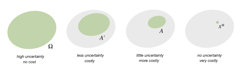
In its most basic form, the concept of decision-making can be formalized as the process of looking for a decision in a discrete set of options . We say that a decision is certain, if repeated queries of the decision-maker will result in the same decision, and it is uncertain, if repeated queries can result in different decisions. Uncertainty reduction then corresponds to reducing the amount of uncertain options. Hence, a decision-making process that transitions from a space of options to a strictly smaller subset reduces the amount of uncertain options from to , with the possible goal to eventually find a single certain decision . Such a process is generally costly, the more uncertainty is reduced the more resources it costs (Figure 1). The explicit mapping between uncertainty reduction and resource cost depends on the details of the underlying process and on which explicit quantity is taken as the resource. For example, if the resource is given by time (or any monotone function of time), then a search algorithm that eliminates options sequentially until the target value is found (linear search) is less cost efficient than an algorithm that takes a sorted list and in each step removes half of the options by comparing the mid point to the target (logarithmic search). Abstractly, any real-valued function on the power set of that satisfies whenever might be used as a cost function in the sense that quantifies the expenses of reducing the uncertainty from to .
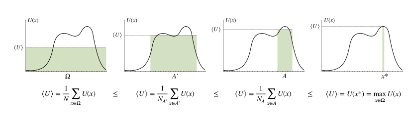
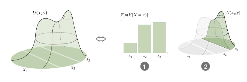
In utility theory decision-making is modelled as an optimization process that maximizes a so-called utility function (which can itself be an expected utility with respect to a probabilistic model of the environment, in the sense of von Neumann and Morgenstern [99]). A decision-maker that is optimizing a given utility function obtains a utility of on average after reducing the amount of uncertain options from to (see Figure 2). A decision-maker that completely reduces uncertainty by finding the optimum is called rational (w.l.o.g. we can assume that is unique, by redefining in the case when it is not). Since uncertainty reduction generally comes with a cost, a utility optimizing decision-maker with limited resources, correspondingly called bounded rational (see Section 3), in contrast will obtain only uncertain decisions from a subset . Such decision-makers seek satisfactory rather than optimal solutions, for example by taking the first option that satisfies a minimal utility requirement, which Herbert Simon calls a satisficing solution [87].
Summarizing, we conclude that a decision-making process with decision space that successively eliminates options can be represented by a mapping between subsets of , together with a cost function that quantifies the total expenses of arriving at a given subset,
| (2.1) |
such that
| (2.2) |
For example, a rational decision-maker can afford , whereas a decision-maker with limited resources can typically only afford uncertainty reduction with cost .
From a probabilistic perspective, a decision-making process as described above is a transition from a uniform probability distribution over options to a uniform probability distribution over options, that converges to the Dirac measure centered at in the fully rational limit. From this point of view, the restriction to uniform distributions is artificial. A decision-maker that is uncertain about the optimal decision might indeed have a bias towards a subset without completely excluding other options (the ones in ), so that the behavior must be properly described by a probability distribution . Therefore, in the following section, we extend (2.1) and (2.2) to transitions between probability distributions. In particular, we must replace the power set of by the space of probability distributions on , denoted by .
2.2. Probabilistic decision-making
Let be a discrete decision space of options, so that consists of discrete distributions , often represented by probability vectors . However, many of the concepts presented in this and the following section can be generalized to the continuous case [62, 44].
Intuitively, the uncertainty contained in a distribution is related to the relative inequality of its entries, the more similar its entries are, the higher the uncertainty. This means that uncertainty is increased by moving some probability weight from a more likely option to a less likely option. It turns out that this simple idea leads to a concept widely known as majorization [36, 10, 72, 13, 62, 11], which has roots in the economic literature of the early 19th century [60, 74, 23], where it was introduced to describe income inequality, later known as the Pigou-Dalton Principle of Transfers. Here, the operation of moving weight from a more likely to a less likely option corresponds to the transfer of income from one individual of a population to a relatively poorer individual (also known as a Robin Hood operation [10]). Since a decision-making process can be viewed as a sequence of uncertainty reducing computations, we call the inverse of such a Pigou-Dalton transfer an elementary computation.
Definition 2.1 (Elementary computation).
A transformation on of the form
| (2.3) |
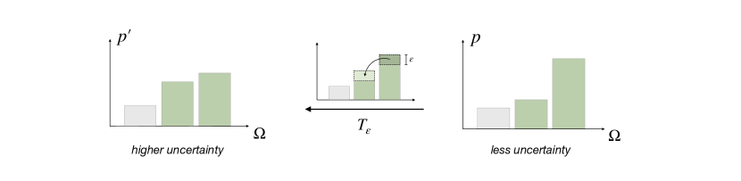
where are such that , and , is called a Pigou-Dalton transfer (see Figure 3). We call its inverse an elementary computation.
Since making two probability values more similar or more dissimilar are the only two possibilities to minimally transform a probability distribution, elementary computations are the most basic principle of how uncertainty is reduced. Hence, we conclude that a distribution has more uncertainty than a distribution if and only if can be obtained from by finitely many elementary computations (and permutations, which are not considered an elementary computation due to the choice of ).
Definition 2.2 (Uncertainty).
We say that contains more uncertainty than , denoted by
| (2.4) |
if and only if can be obtained from by a finite number of elementary computations and permutations.
Note that, mathematically this defines a preorder on , i.e. a reflexive ( for all ) and transitive (if , then for all ) binary relation.
In the literature, there are different names for the relation between and expressed by Definition 2.2, for example is called more mixed than [79], more disordered than [78], more chaotic than [13], or an average of [36]. Most commonly however, is said to majorize , which started with the early influences of Muirhead [65], and Hardy, Littlewood, and Pólya [36] and was developed by many authors into the field of majorization theory (a standard reference is by Marshall, Olkin, and Arnold [62]), with far reaching applications until today, especially in nonequilibrium thermodynamics and quantum information theory [15, 41, 34].
There are plenty of equivalent (arguably less intuitive) characterizations of , some of which we are summarizing below. However, one characterization makes use of a concept very closely related to Pigou-Dalton transfers, known as T-transforms [13, 62], which expresses the fact that moving some weight from a more likely option to a less likely option is equivalent to taking (weighted) averages of the two probability values. More precisely, a T-transform is a linear operator on with a matrix of the form , where denotes the identity matrix on , denotes a permutation matrix of two elements, and . If permutes and , then for all , and
| (2.5) |
Hence, a T-transform considers any two probability values and of a given , calculates their weighted averages with weights and , and replaces the original values with these averages. From (2.5) it follows immediately that a T-transform with parameter and a permutation of with is a Pigou-Dalton transfer with . Also allowing means that T-transfers include permutations, in particular, if and only if can be derived from by successive applications of finitely many T-transforms
Due to a classic result by Hardy, Littlewood and Pólya [36, p.49], this characterization can be stated in an even simpler form by using doubly stochastic matrices, i.e. matrices with and for all . By writing for all , and , these conditions are often stated as
| (2.6) |
Note that doubly stochastic matrices can be viewed as generalizations of T-transforms in the sense that a T-transform takes an average of two entries, whereas if with a doubly stochastic matrix , then is a convex combination, or a weighted average, of with coefficients for each . This is also, why is then called more mixed than [79]. Therefore, similar to T-transforms, we might expect that if is the result of an application of a doubly stochastic matrix, , then is an average of and therefore contains more uncertainty than . This is exactly what is expressed by characterization in the following theorem. A similar characterization of is that must be given by a convex combination of permutations of the elements of (see property below).
Without having the concept of majorization, Schur proved that functions of the form with a convex function are monotone with respect to the application of a doubly stochastic matrix [83] (see property below). Functions of this form are an important class of cost functions for probabilistic decision-makers, as we will discuss in Example Example.
Theorem 2.3 (Characterizations of [62]).
For , the following are equivalent:
-
, i.e. contains more uncertainty than (Definition 2.2)
-
is the result of finitely many T-transforms applied to
-
for a doubly stochastic matrix
-
where , , , and is a permutation for all
-
for all continuous convex functions
-
for all , where denotes the decreasing rearrangement of .
As argued above, the equivalence between and is straight-forward. The equivalences between , , and are due to Muirhead [65] and Hardy, Littlewood, and Pólya [36]. The implication is due to Karamata [47] and Hardy, Littlewood, and Pólya [37], whereas goes back to Schur [83]. Mathematically, means that belongs to the convex hull of all permutations of the entries of , and the equivalence is known as the Birkhoff-von Neumann theorem. Here, we have stated all relations for probability vectors , even though they are usually stated for all with the additional requirement that .
Condition is the classical and most commonly used definition of majorization [60, 36, 62], since it is often the easiest to check in practical examples. For example, from it immediately follows that uniform distributions over options contain more uncertainty than uniform distributions over options, since we have for all , i.e. for it follows that
| (2.7) |
In particular, if , then the uniform distribution over contains less uncertainty than the uniform distribution over , which shows that the notion of uncertainty introduced in Definition 2.2 is indeed a generalizatin of the notion of uncertainty given by the number of uncertain options introduced in the previous section.
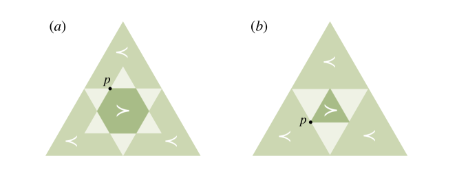
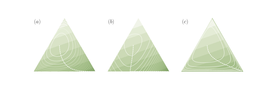
Note that, only being a preorder on , in general, two distributions are not necessarily comparable, i.e. we can have both and . In Figure 4, we visualize the regions of all comparable distributions for two exemplary distributions on a three-dimensional decision space (), represented on the two-dimensional simplex of probability vectors . For example,
can not be compared under , since , but .
Cost functions can now be generalized to probabilistic decision-making by noting that the property whenever in (2.2) means that is strictly monotonic with respect to the preorder given by set inclusion.
Definition 2.4 (Cost functions on ).
We say that a function is a cost function, if it is strictly monotonically increasing with respect to the preorder , i.e. if
| (2.8) |
with equality only if and are equivalent, , which is defined as and . Moreover, for a parametrized family of posteriors , we say that is a resource parameter with respect to a cost function , if the mapping is strictly monotonically increasing.
Since monotonic functions with respect to majorization were first studied by Schur [83], functions with this property are usually called (strictly) Schur-convex [62, Ch. 3].
Example (Generalized entropies).
From in Theorem 2.3 it follows that functions of the form
| (2.9) |
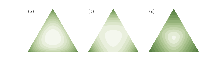
where is strictly convex, are examples of cost functions. Since many entropy measures used in the literature can be seen to be special cases of (2.9) (with a concave ), functions of this form are often called generalized entropies [18]. In particular, for the choice , we have , where denotes the Shannon entropy of . Thus, if contains more uncertainty than in the sense of Definition 2.2 () then the Shannon entropy of is larger than the Shannon entropy of and therefore contains also more uncertainty in the sense of classical information theory than . Similarly, for we obtain the (negative) Burg entropy, and for functions of the form for we get the (negative) Tsallis entropy, where the sign is chosen depending on such that is convex (see e.g. [32] for more examples). Moreover, the composition of any (strictly) monotonically increasing function with (2.9) generates another class of cost functions, which contains for example the (negative) Rényi entropy [77]. Note also that entropies of the form (2.9) are special cases of Csiszár’s f-divergences [20] for uniform reference distributions (see Example Example below). In Figure 5, several examples of cost functions are shown for . In this case, the 2-dimensional probability simplex is given by the triangle in with edges , , and . Cost functions are visualized in terms of their level sets.
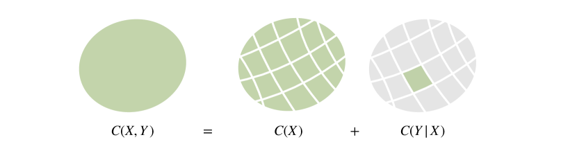
We prove in Proposition A.1 in the appendix that all cost functions of the form (2.9) are superadditive with respect to coarse-graining. This seems to be a new result and an improvement upon the fact that generalized entropies (and -divergences) satisfy information monotonicity [5]. More precisely, if a decision in , represented by a random variable , is split up into two steps by partitioning and first deciding about the partition , correspondingly described by a random variable with values in , and then choosing an option inside of the selected partition , represented by a random variable , i.e. , then
| (2.10) |
where and . For symmetric cost functions (such as (2.9)) this is equivalent to
| (2.11) |
The case of equality in (2.10) and (2.11) (see Figure 6) is sometimes called separability [51], strong additivity [21], or recursivity [4], and it is often used to characterize Shannon entropy [26, 96, 48, 55, 77, 2]. In fact, we also show in the appendix (Proposition A.2) that cost functions that are additive under coarse-graining are proportional to the negative Shannon entropy . See also Example Example in the next section, where we discuss the generalization to arbitrary reference distributions.
We can now refine the notion of a decision-making process introduced in the previous section as a mapping together with a cost function satisfying (2.2). Instead of simply mapping from sets to smaller subsets by successively eliminating options, we now allow to be a mapping between probability distributions such that can be obtained from by a finite number of elementary computations (without permutations), and we require to be a cost function on , so that
| (2.12) |
Here, quantifies the total costs of arriving at a distribution , and means that and . In other words, a decision-making process can be viewed as traversing probability space by moving pieces of probability from one option to another option such that uncertainty is reduced.
Up to now we have ignored one important property of a decision-making process, the distribution with minimal cost, i.e. satisfying for all , which must be identified with the initial distribution of a decision-making process with cost function . As one might expect (see Figure 5), it turns out that all cost functions according to Definition 2.4 have the same minimal element.
Proposition 2.5 (Uniform distributions are minimal).
The uniform distribution is the unique minimal element in with respect to , i.e.
| (2.13) |
Once (2.13) is established, it follows from (2.8) that for all , in particular the uniform distribution corresponds to the initial state of all decision-making processes with cost function satisfying (2.12). In particular, it contains the maximum amount of uncertainty with respect to any entropy measure of the form (2.9), known as the second Khinchin axiom [51], e.g. for Shannon entropy . Proposition 2.5 follows from characterization in Theorem 2.3 after noticing that every can be transformed to a uniform distribution by permuting its elements cyclically (see Proposition A.3 in the appendix for a detailed proof).
Regarding the possibility that a decision-maker may have prior information, for example originating from the experience of previous comparable decision-making tasks, the assumption of a uniform initial distribution seems to be artificial. Therefore, in the following section we arrive at the final notion of a decision-making process by extending the results of this section to allow for arbitrary initial distributions.
2.3. Decision-making with prior knowledge
From the discussion at the end of the previous section we conclude that, in full generality, a decision-maker transitions from an initial probability distribution , called prior, to a terminal distribution , called posterior. Note that, since once eliminated options are excluded from the rest of the decision-making process, a posterior must be absolutely continuous with respect to the prior , denoted by , i.e. can be non-zero for a given only if is non-zero.
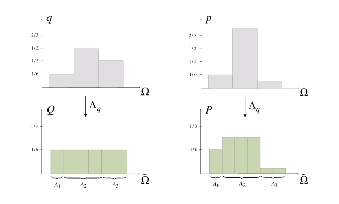
The notion of uncertainty (Definition 2.2) can be generalized with respect to a non-uniform prior by viewing the probabilities as the probabilities of partitions of an underlying elementary probability space of equally likely elements under , in particular represents as the uniform distribution on (see Figure 7). The similarity of the entries of the corresponding representation of any (its uncertainty) then contains information about how close is to , which we call the relative uncertainty of with respect to (Definition 2.6 below).
The formal construction is as follows: Let be such that and . The case when then follows from a simple approximation of each entry by a rational number. Let be such that for all , for example could be chosen as the least common multiple of the denominators of the . The underlying elementary probability space then consists of elements and there exists a partitioning of such that
| (2.14) |
where denotes the uniform distribution on . In particular, it follows that
| (2.15) |
i.e. represents in with respect to the partitioning . Similarly, any can be represented as a distribution on by requiring that for all and letting to be constant inside of each partition, i.e. similar to (2.15) we have for all and therefore by (2.14)
| (2.16) |
Note that, if then by absolute continuity () in which case we can either exclude option from or set .
Example.
For a prior we put , so that should be partitioned as . Then corresponds to the probability of the -th partition under the uniform distribution , while is represented on by (see Figure 7).
Importantly, if the components of the representation in given by (2.16) are similar to each other, i.e. if is close to uniform, then the components of must be very similar to the components of , which we express by the concept of relative uncertainty.
Definition 2.6 (Uncertainty relative to ).
We say that contains more uncertainty with respect to a prior than , denoted by , if and only if contains more uncertainty than , i.e.
| (2.17) |
where is given by (2.16).
As we will show in Theorem 2.7 below, it turns out that coincides with a known concept called -majorization [97], majorization relative to [44, 62], or mixing distance [80]. Due to the lack of a characterization by partial sums, it is usually defined as a generalization of characterization in Theorem 2.3, that is is -majorized by iff , where is a so-called -stochastic matrix, which means that it is a stochastic matrix () with . In particular, does not depend on the choice of in the definition of . Here, we provide two new characterizations of -majorization, the one given by Definition 2.6, and one using partial sums generalizing the original definition of majorization.
Theorem 2.7 (Characterizations of ).
The following are equivalent
-
, i.e. contains more uncertainty relative to than (Def. 2.6)
-
can be obtained from by a finite number of elementary computations and permutations on
-
for a -stochastic matrix , i.e. and
-
for all continuous convex functions
-
for all that satisfy and , where the arrows indicate that is ordered decreasingly, and .
To prove that , , and are equivalent (see Proposition A.4 in the appendix), we use of the fact that has a left inverse . This can be verified by simply multiplying the corresponding matrices given in the proof of Proposition A.4. The equivalence betweeen and is shown in [44] (see also [80, 62]). Characterization follows immediately from Definition 2.2 and Definition 2.6.
As required from the discussion at the end of the previous section, is indeed minimal with respect to , which means that it contains the most amount of uncertainty with respect to itself.
Proposition 2.8 (The prior is minimal).
The prior is the unique minimal element in with respect to , that is
| (2.18) |
This follows more or less directly from Proposition 2.5 and the equivalence of and in Theorem 2.7 (see Proposition A.5 in the appendix for a detailed proof).
Order-preserving functions with respect to generalize cost functions introduced in the previous section (Definition 2.4). According to Proposition 2.8, such functions have a unique minimum given by the prior . Since cost functions are used in Definition 2.11 below to quantify the expenses of a decision-making process, we require their minimum to be zero, which can always be achieved by redefining a given cost function by an additive constant.
Definition 2.9 (Cost functions relative to ).
We say that a function is a cost function relative to , if , if it is invariant under relabeling , and if it is strictly monotonically increasing with respect to the preorder , that is if
| (2.19) |
with equality only if , i.e. if and . Moreover, for a parametrized family of posteriors , we say that is a resource parameter with respect to a cost function , if the mapping is strictly monotonically increasing.
Similar to generalized entropy functions discussed in Example Example, in the literature there are many examples of relative cost functions, usually called divergences or measures of divergence.
Example (-divergences).
From in Theorem 2.7 it follows that functions of the form
| (2.20) |
where is continuous and strictly convex with , are examples of cost functions relative to . Many well-known divergence measures can be seen to belong to this class of relative cost functions, also known as Csiszár’s -divergences [20]: the Kullback-Leibler divergence (or relative entropy), the squared distance, the Hartley entropy, the Burg entropy, the Tsallis entropy, and many more [32, 21] (see Figure 8 for visualizations of some of them in relative to a non-uniform prior).
As a generalizition of Proposition A.1 (superadditivity of generalized entropies), we prove in Proposition A.6 in the appendix that -divergences are superadditive under coarse-graining, that is, for
| (2.21) |
whenever and . This generalizes (2.10) to the case of a non-uniform prior. Similar to entropies, the case of equality in (2.21) is sometimes called composition rule [40], chain rule [57], or recursivity [21], and is often used to characterize Kullback-Leibler divergence [40, 63, 21, 57].
Indeed, we also show in the appendix (Proposition A.7) that all additive cost functions with respect to are proportional to Kullback-Leibler divergence (relative entropy). This goes back to Hobson’s modification [40] of Shannon’s original proof [85], after establishing the following monotonicity property for uniform distributions: If denotes the cost of a uniform distribution over elements relative to a uniform distribution over elements, then (see Figure 9)
| (2.22) |
Note that, even though our proof of Proposition A.7 uses additivity under coarse graining to show the monotonicity property (2.22), it is easy to see that any relative cost function of the form (2.20) also satisfies (2.22) by using the convexity of in the form with .

In terms of decision-making, superadditivity under coarse-graining means that decision-making costs can potentially be reduced by splitting up the decision into multiple steps, for example by a more intelligent search strategy. For example, if for some and is superadditive, then the cost for reducing uncertainty to a single option, i.e. , when starting from a uniform distribution , satisfies
where , and we have set as unit cost (corresponding to 1 bit in the case of Kullback-Leibler divergence). Thus, intuitively the property of the Kullback-Leibler divergence of being additive under coarse-graining might be viewed as describing the minimal amount of processing costs that must be contained in any cost function, because it cannot be reduced by changing the decision-making process. Therefore, in the following we call cost functions that are proportional to the Kullback-Leibler divergence simply informational costs.
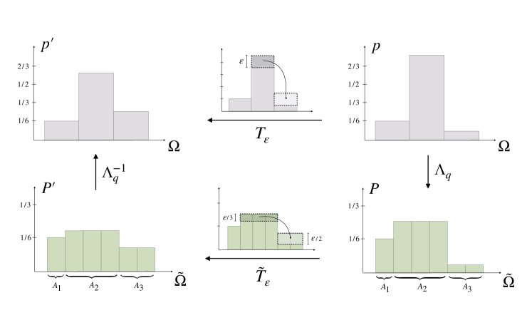
In contrast to the previous section, in the definition of and its characterizations we have never used elementary computations on directly. This is due to the fact that permutations do interact with the uncertainty relative to , and therefore cannot be characterized by a finite number of elementary computations and permutations on . However, we can still define elementary computations relative to by the inverse of Pigou-Dalton transfers of the form (2.3) such that for , which is arguably the most basic form of how to generate uncertainty with respect to .
Even for small , a regular Pigou-Dalton transfer does not necessarily increase uncertainty relative to , because the similarity of the components now needs to be considered with respect to . Instead, we compare the components of the representation of , and move some probability weight from to whenever for and , by distributing evenly among the elements in (see Figure 10), denoted by the transformation . Here, must be small enough such that the inequality is invariant under , which means that
and therefore
| (2.23) |
By construction, minimally increases uncertainty in while staying in the image of under , by keeping the values of constant in each partition, and therefore can be considered as the most basic way of how to increase uncertainty relative to .
Definition 2.10 (Elementary computation relative to ).
We call a transformation on of the form
| (2.24) |
with such that , and satisfying (2.23), a Pigou-Dalton transfer relative to , and its inverse an elementary computation relative to .
We are now in the position to state our final definition of a decision-making process.
Definition 2.11 (Decision-making process).
A decision-making process is a gradual transformation
of a prior to a posterior , such that each step decreases uncertainty relative to . This means that is obtained from by successive application of a mapping between probability distributions on , such that can be obtained from by finitely many elementary computations relative to , in particular
| (2.25) |
where quantifies the total costs of a distribution , and means that and .
In other words, a decision-making process can be viewed as traversing probability space from prior to posterior by moving pieces of probability from one option to another option such that uncertainty is reduced relative to , while expending a certain amount of resources determined by the cost function .
3. Bounded rationality
3.1. Bounded rational decision-making
In this section, we consider decision-making processes that trade off utility against costs. Such decision-makers either maximize a utility function subject to a constraint on the cost function, for example an author of a scientific article that optimizes the article’s quality until a deadline is reached, or minimizing the cost function subject to a utility constraint, for example a high-school student that minimizes effort such that the requirement to pass a certain class is achieved. In both cases, the decision-makers are called bounded rational, since in the limit of no resource constraints they coincide with rational decision-makers.
In general, depending on the underlying system, such an optimization process might have additional process dependent constraints that are not directly given by resource limitations, for example in cases when the optimization takes place in a parameter space that has less degrees of freedom than the full probability space . Abstractly, this is expressed by allowing the optimization process to search only in a subset .
Definition 3.1 (Bounded rational decision-making process).
Let be a given utility function, and . A decision-making process with prior , posterior , and cost function is called bounded rational if its posterior satisfies
| (3.1) |
for a given upper bound , or equivalently
| (3.2) |
for a given lower bound . In the case when the process constraints disappear, i.e. if , then a bounded rational decision-maker is called bounded-optimal.
The equivalence between (3.1) and (3.2) is easily seen from the equivalent optimization problem given by the formalism of Lagrange multipliers [25],
| (3.3) |
where the cost or utility constraint is expressed by a trade-off between utility and cost, or cost and utility, with a trade-off parameter given by the Lagrange multiplier , which is chosen such that the constraint given by or is satisfied. It is easily seen from the maximization problem on the right side of (3.3) that a larger value of decreases the weight of the cost term and thus allows for higher values of the cost function. Hence, parametrizes the amount of resources the decision-maker can afford with respect to the cost function , and, at least in non-trivial cases (non-constant utilities) it is therefore a resource parameter with respect to in the sense of Definition 2.9. In particular, for , the decision-maker minimizes its cost function irrespective of the expected utility, and therefore stays at the prior, , whereas makes the cost function disappear so that the decision-maker becomes purely rational with a Dirac posterior centered on the optima of the utility function .
For example, in Figure 11 we can see how the posteriors of bounded-optimal decision-makers with different cost functions for and with utility leave a trace in probability space, by moving away from an exemplary prior and eventually arriving at the rational solution .
For informational costs (i.e. proportional to Kullback-Leibler divergence), is a resource parameter with respect to any cost function.
Proposition 3.2.
If is a family of bounded-optimal posteriors given by (3.3) with , then is a resource parameter with respect to any cost function, in particular
| (3.4) |
This generalizes a result in [78] to the case of non-uniform priors, by making use of our new characterization of , by which it suffices to show that the function is monotonically increasing for all specified in Theorem 2.7 (see Proposition A.8 in the appendix for details). For simplicity, we restrict ourselves to the case of the Kullback-Leibler divergence, however the proof is analogous for cost functions of the form (2.20) with being differentiable and strictly convex on (so that is strictly monotonically increasing and thus invertible on , see [78] for the case of uniform priors).
Hence, for any , the posteriors of a bounded-optimal decision-making process with the Kullback-Leibler divergence as cost function can be regarded as the steps of a decision-making process (i.e. satisfying (2.25)) with posterior , where each step optimally trades off utility against informational cost. This means that with increasing the posteriors do not only decrease entropy in the sense of the Kullback-Leibler divergence, but also in the sense of any other cost function.
The important case of bounded-optimal decision-makers with informational costs is termed information-theoretic bounded rationality [68, 92, 70] and is studied more closely in the following sections.
3.2. Information-theoretic bounded rationality
For bounded-optimal decision-making processes with informational costs the unconstrained optimization problem (3.3) takes the form , where
| (3.5) |
which has a unique maximum , the bounded-optimal posterior given by
| (3.6) |
with normalization constant . This form can easily be derived by finding the zeros of the functional derivative of the objective functional (3.5) with respect to (with an additional normalization constraint), whereas the uniqueness follows from the convexity of the mapping . For the actual maximum of we obtain
so that .
Due to its analogy with physics, in particular thermodynamics (see e.g. [70]), the maximization of (3.5) is known as the Free Energy principle of information-theoretic bounded rationality, pioneered in [68, 92, 70], further developed in [29, 33], and applied in recent studies of artificial systems, such as generative neural networks trained by Markov chain Monte Carlo methods [38], or in reinforcement learning as an adaptive regularization strategy [56, 35], as well as in recent experimental studies on human behavior [71, 82]. Note that there is a formal connection of (3.5) and the Free Energy principle of active inference [28], however, as discussed in [33, Sec. 6.3], both Free Energy principles have conceptually different interpretations.
Example (Bayes rule as a bounded-optimal posterior).
In Bayesian inference, the parameter of the distribution of a random variable is inferred from a given dataset of observations of by treating the parameter itself as a random variable with a prior distribution . The parametrized distribution of evaluated at an observation given a certain value of , i.e. , is then understood as a function of , known as the likelihood of the datapoint under the assumption of . After seeing the dataset , the belief about is updated by using Bayes rule
This takes the form of a bounded-optimal posterior (3.6) with and utility function given by the average log-likelihood per datapoint,
since then Bayes rule reads
| (3.7) |
coincides with the variational Free Energy from Bayesian statistics. Indeed, from (3.8) it is easy to see that assumes its maximum when is proportional to , that is when is given by (3.7). In the literature, is used in the variational characterization of Bayes rule, in cases when the form (3.7) cannot be achieved exactly but instead is approximated by optimizing (3.8) over the parameters of a parametrized distribution [39, 61].
In the following section, we will see that the Free Energy of a bounded rational decision-making process satisfies a recursivity property, which allows the interpretation of as a certainty-equivalent.
3.3. The recursivity of and the value of a decision problem
Consider a bounded-optimal decision-maker with an informational cost function deciding about a random variable with values in that is decomposed into the random variables and , i.e. . This decomposition can be understood as a two-step process, where first a decision about a partition of the full search space is made, represented by a random variable with values in , followed by a decision about inside the partition selected by (see Figure 6).
Since , by the additivity of the Kullback-Leibler divergence (Proposition A.7), we have
and therefore, if denotes the Free Energy of the second step,
| (3.9) |
In particular, the Free Energy of the second decision-step plays the role of the utility function of the first decision-step (see Figure 12). In Equation (3.9), the two decision-steps have the same resource parameter , controlling the strength of the constraint on the total informational costs
More generally, each step might have a separate information-processing constraint, which requires two resource parameters and , and results in the total Free Energy
Example.
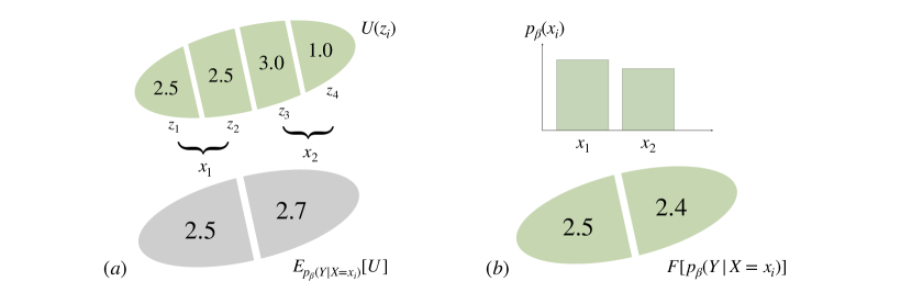
Consider a bounded-rational decision-maker with informational cost function and a utility function defined on a set with values as given in Figure 13 and an information-processing bound of bits (). If we partition into the disjoint subsets and , then the decision about can be decomposed into two steps, , the decision about corresponding to the choice of the partition and the decision about given corresponding to the choice of inside the given partition determined by . According to Equation (3.9), the choice of the partition is not in favor of the achieved expected utility inside each partition, but of the Free Energy (see Figure 13).
Therefore, a bounded rational decision-maker that has the choice among decision-problems ideally should base its decision not on the expected utility that might be achieved but on the Free Energy of the subordinate problems. In other words, the Free Energy quantifies the value of a decision-problem, that besides of the achieved average utility also takes the information-processing costs into account.
3.4. Multi-task decision-making and the optimal prior
So far, we have considered decision-making problems with utility functions defined on only, modelling a single decision-making task. This is extended to multi-task decision-making problems by utility functions of the form , where the additional variable represents the current state of the world. Different world states in general lead to different optimal decisions . For example, in a chess game the optimal moves depend on the current board configurations the players are faced with.
The prior for a bounded-rational multi-task decision-making problem may either depend or not depend on the world state . In the first case, the multi-task decision-making problem is just given by multiple single-task problems, i.e. for each , and are the prior and posterior of a bounded rational decision-making process with utility function , as described in the previous sections. In the case when there is a single prior for all world states , the Free Energy is
| (3.10) |
where is a given world state distribution. Note that, for simplicity we assume that is independent of , which means that only the average information-processing is constrained, in contrast to the information-processing being constrained for each world state which in general would result in being a function of . Similarly to single-task decision-making (Equation (3.6)) the maximum of (3.10) is achieved by
| (3.11) |
with normalization constant . Interestingly, the deliberation cost in (3.10) depends on how well the prior was chosen to reach all posteriors without violating the processing constraint. In fact, viewing the Free Energy (3.10) as a function of both, posterior and prior, , and optimizing for the prior yields the marginal of the joint distribution , i.e. the mean of the posteriors for the different world states,
| (3.12) |
Similarly to (3.6), Equation (3.12) follows from finding the zeros of the functional derivative of the Free Energy with respect to (modified by an additional term for the normalization constraint).
Optimizing the Free Energy for both prior and posterior can be achieved by iterating Equations (3.11) and (3.12). This results in an alternating optimization algorithm, originally developed independently by Blahut and Arimoto to calculate the capacity of a memoryless channel [14, 9] (see [22] for a convergence proof by Csiszár and Tusnády). Note that
in particular, that the information-processing cost is now given by the mutual information between the random variables and . In this form, we can see that the Free Energy optimization with respect to prior and posterior is equivalent to the optimization problem in classical rate distortion theory [86], where is given by the negative of the distortion measure.
Similarly as in rate-distortion theory, where compression algorithms are anaylized with respect to the rate-distortion function, any decision-making system can now be analyzed with respect to informational bounded-optimality. More precisely, when plotting the achieved expected utility against the information-processing resources of a bounded-rational decision-maker with optimal prior, we obtain a pareto-optimality curve that forms an efficiency-frontier that cannot be surpassed by any decision-making process (see Figure 14).
3.5. Multi-task decision-making with unknown world state distribution
A bounded rational decision-making process with informational cost and utility that has an optimal prior given by the marginal (3.12) must have perfect knowledge about the world state distribution . In contrast, here we consider the case when the exact shape of the world state distribution is unknown to the decision-maker and therefore has to be inferred from the already seen world states. More precisely, we assume that the world state distribution is parametrized by a parameter , i.e. for a given parametrized distribution . Since the true parameter is unknown, is treated as a random variable by itself, so that . After a dataset of samples from has been observed the joint distribution of all involved random variables can be written as
where denotes the decision-maker’s prior belief about , and is the likelihood of the previously observed world states. Therefore, the resulting (multi-task) Free Energy (see Equation (3.10)) is given by
| (3.13) |
It turns out that we obtain Bayesian inference as a byproduct of optimizing (3.13) with respect to the prior . Indeed, by calculating the functional derivative with respect to of the Free Energy (3.13) plus an additional term for the normalization constraint of (with Lagrange multiplier ), we can see that any distribution that optimizes (3.13) must satisfy
where is chosen such that for any . This is equivalent to
where denotes the normalization constant of , given by , since as well as . Therefore, we obtain
with as defined in Equation (3.14). Hence, we have shown
Proposition 3.3 (Optimality of Bayesian inference).
The optimal prior that maximizes (3.13) is given by , where is the Bayes posterior
| (3.14) |
4. Example: Absolute identification task with known and unknown stimulus distribution
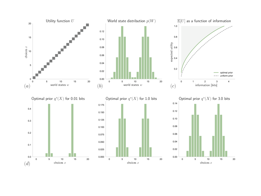
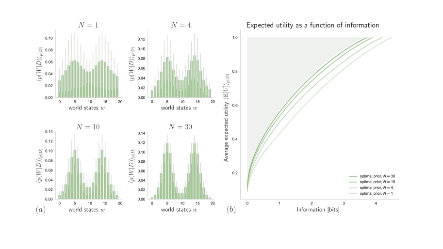
Consider a bounded rational decision-maker with a multi-task utility function such that for each , is non-zero for only one choice as shown in Figure 14. Here, the decision and world spaces are both finite sets of elements. The world state distribution is given by a mixture of two Gaussian distributions as shown in Figure 14. Due to some world states being more likely than others, there are some choices that are less likely to be optimal.
4.1. Known stimulus distribution
As can be seen in Figure 14 (dashed line), here it is not ideal to have a uniform prior distribution, for all . Instead, if the world state distribution is known perfectly and the prior has the form suggested by Equation (3.12), i.e. , then, as can be seen in Figure 14 (solid line), achieving the same expected utility as with a uniform prior requires less informational resources. In particular, the explicit form of depends on the resource parameter , see Figure 14. For low resource availability (small ), only the choices that correspond to the most probable world states are considered. However, for , we have
because here is the posterior of a rational decision-maker, where denotes the Kronecker- (which is only non-zero if ). Hence, for decision-makers with abundant information-processing resources (large ) the optimal prior approaches the form of the world state distribution (since here ).
4.2. Unknown stimulus distribution
In the case when the decision-maker has to infer its knowledge about from a set of samples , we know from Section 3.5 that this is optimally done via Bayesian inference. Here, we assume a mixture auf two Gaussians as a parametrization of , so that , where and denote mean and standard-deviation of the -th component respectively (for simplicity, with fixed equal weights for the two mixture components).
In Figure 15, we can see how different values of affect the belief about the world state distribution, , when is given by the Bayes posterior (3.14) with a uniform prior belief . The resulting expected utilities (averaged over samples from ) as functions of available information-processing resources are displayed in Figure 15, which shows how the performance of a bounded-rational decision-maker with optimal prior and perfect knowledge about the true world state distribution is approached by bounded rational decision-makers with limited but increasing knowledge given by the sample size .
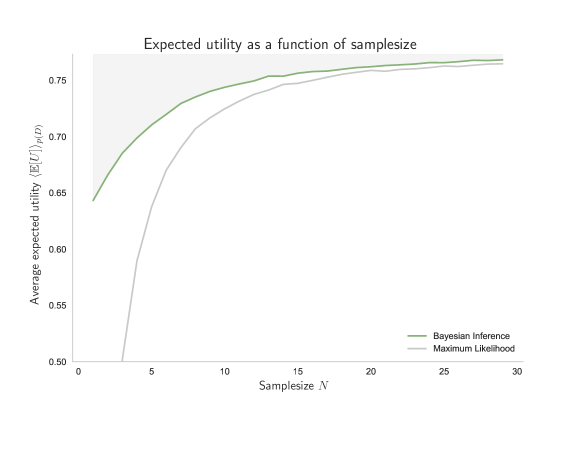
Abstractly, we can view Equation (3.14) as the bounded optimal solution to the decision-making problem that starts with a prior and arrives at a posterior after processing the samples in (see also Example Example). In fact, the posteriors shown in Figure 15 satisfy the requirements for a decision-making process with resource given by the number of datapoints , when averaged over . In particular, by increasing the posteriors contain less and less uncertainty with respect to the preorder given by majorization. Accordingly, if we plot the achieved expected utility against the number of samples, we obtain an optimality curve similar to Figure 14 and Figure 15. In Figure 16 we can see how Bayesian Inference outperforms Maximum Likelihood when evaluated with respect to the average expected utility of a bounded-rational decision-maker with bits of information-processing resources.
5. Discussion
In this work, we have developed a generalized notion of decision-making in terms of uncertainty reduction. Based on the simple idea of transferring pieces of probability between the elements of a probability distribution, which we call elementary computations, we have promoted a notion of uncertainty which is known in the literature as majorization, a preorder on . Taking non-uniform initial distributions into account, we extended the concept to the notion of relative uncertainty, which corresponds to relative majorization . Despite of the large amount of research that has been done on majorization theory, from the early works [65, 60, 36] through further developments [79, 10, 8, 72, 19, 13, 62] to modern applications [15, 41, 34], there is a lack of results on the more general concept of relative majorization. This does not seem to be due to a lack of interest, as can be seen from the results [97, 80, 44, 54], but mostly because relative majorization looses some of the appealing properties of majorization which makes it harder to deal with, for example that permutations no longer leave the ordering invariant, in contrast to the case of a uniform prior. This restriction does, however, not affect our application of the concept to decision-making, as permutations are not considered as elementary computations, since they do not diminish uncertainty. By reducing the non-uniform to the uniform case, we managed to prove new results on relative majorization (Theorem 2.7), which then enabled new results in other parts of the paper (Example Example, Propositions A.6, A.8), and allowed an intuitive interpretation of our final definition of a decision-making process (Definition 2.11) in terms of elementary computations with respect to non-uniform priors (Definition 2.10).
More precisely, starting from stepwise elimination of uncertain options (Section 2.3), we have argued that decision-making can be formalized by transitions between probability distributions (Section 2.2), and arrived at the concept of decision-making processes traversing probability space from prior to posterior by successively moving pieces of probability between options such that uncertainty relative to the prior is reduced (Section 2.1). Such transformations can be quantified by cost functions, which we define as order-preserving functions with respect to and capture the resource costs that must be expended by the process. We have shown (Propositions A.1, A.6) that many known generalized entropies and divergences, which are examples of such cost functions (Examples Example and Example), satisfy superadditivity with respect to coarse-graining. This means that under such cost functions, decision-making costs can potentially be reduced by a more intelligent search strategy, in contrast to Kullback-Leibler divergence, which was characterized as the only additive cost function (Proposition A.7). There are plenty of open questions for further investigation in that regard. First, it is not clear under which assumptions on the cost functions superadditivity could be improved to with and . Additionally, it would be an interesting challenge to find sufficient conditions implying super-additivity that include more cost functions than -divergences. The field of information geometry might give further insights on the topic, since there are studies in similar directions, in particular characterizations of divergence measures in terms of information monotonicity and the data-processing inequality [43, 5, 6, 7]. One interesting result is the characterization of Kullback-Leibler divergence as the single divergence measure being both an -divergence and a Bregman divergence.
In Section 3, bounded rational decision-makers were defined as decision-making processes that are maximizing utility under constraints on the cost function, or equivalently minimizing resource costs under a minimal utility requirement. In the important case of additive cost functions (i.e. proportional to Kullback-Leibler divergence), this leads to information-theoretic bounded rationality [68, 92, 70, 29, 33], which has precursors in the economic and game-theoretic literature [64, 66, 63, 101, 90, 42, 93, 91, 92, 46, 100, 58]. We have shown that the posteriors of a bounded rational decision-maker with increasing informational constraints leave a path in probability space that can itself be considered an anytime decision-making process, in each step perfectly trading off utility against processing costs (Prop. 3.2). In particular, this means that the path of a bounded rational decision-maker with informational cost decreases uncertainty with respect to all cost functions, not just Kullback-Leibler divergence. We have also studied the role of the prior in bounded rational multi-task decision-making, where we have seen that imperfect knowledge about the world state distribution leads to Bayesian inference as a byproduct, which is in line with the characterization of Bayesian inference as minimizing prediction surprise [69], but also demonstrates the wide applicability of the developed theory of decision-making with limited resources.
Finally, in Section 4, we have presented the results of a simulated bounded rational decision-maker solving an absolute identification task with and without knowledge about the world state distribution. Additionally, we have seen that Bayesian inference can be considered a decision-making process with limited resources by itself, where the resource is given by the number of available datapoints.
6. Conclusion
To our knowledge, this is the first principled approach to decision-making based on the intuitive idea of Pigou-Dalton-type probability transfers (elementary computations). Information-theoretic bounded rationality has been introduced by other axiomatic approaches before [68, 63]. For example, in [68] a precise relation between rewards and information value was derived by postulating that systems will choose those states with high probability that are desirable for them. This leads to a direct coupling of probabilities and utility, where utility and information inherit the same structure, and only differ with respect to normalization—see [17] for similar ideas. In contrast, we assume utility and probability to be independent objects a priori that only have a strict relationship in the case of bounded-optimal posteriors. The approach in [63] introduces Kullback-Leibler divergence as disutility for decision control. Based on Hobson’s characterization [40], the authors argue that cost functions should be monotonic with respect to uniform distributions (property (2.22)) and invariant under decomposition, which coincides with additivity under coarse-graining (see Examples Example, Example). Both of these assumptions are special cases of our more general treatment, where cost functions must be monotonic with respect to elementary computations and are generally not restricted to being additive.
In the literature, there are many mechanistic models of decision-making that instantiate decision-making processes with limited resources. Examples include reinforcement learning algorithms with variable depth [49, 50], Markov chain Monte Carlo (MCMC) models where only a certain number of samples can be evaluated [100, 67, 38], and evidence accumulation models that accumulate noisy evidence until either a fixed threshold is reached [53, 75, 94, 76, 84] or where thresholds are determined dynamically by explicit cost functions depending on the number of allowed evidence accumulation steps [27, 24]. Many of these concrete models may be described abstractly by resource parameterizations (Def. 2.9). More precisely, in such cases the posteriors are generated by an explicit process with process constraints and resource parameter . For example, in diffusion processes may correspond to the amount of time allowed for evidence accumulation, in Monte Carlo algorithms may reflect the number of MCMC steps, and in a reinforcement learning agent may represent the number of forward-simulations. If the resource restriction is described by a monotonic cost function [27, 24], then the process can be optimized by a maximization problem of the form
where are non-negative constants, denotes the subset of probability distributions with resource , and denotes a cost function such that for is strictly monotonically increasing. In particular, such cases can also be regarded as bounded rational decision-making problems of the form (3.1).
Bounded rationality models in the literature come in a variety of flavors. In the heuristics and biases paradigm the notion of optimization is often dismissed in its entirety [31], even though decision-makers still have to have a notion of options being better or worse, for example in order to adapt their aspiration levels in a satisficing scheme [88]. We have argued that from an abstract normative perspective we can formulate satisficing in probabilistic terms, such that one could investigate the efficiency of heuristics within this framework. Another prominent approach to bounded rationality is given by systems capable of decision-making about decision-making, i.e. meta-decision-making. Explicit decision-making processes composed of two decision steps have been studied, for example, in the reinforcement learning literature [49, 50, 73, 98], where the first step is represented by a meta decision about whether a cheap model-free or a more expensive model-based learning algorithm is used in the second step. The meta step consists of a trade-off between the estimated utility against the decision-making costs of the second decision step. In the information-theoretic framework of bounded rationality this could be seen as a natural property of multi-step decision-making and the recursivity property (3.9) from which follows that the value of a decision-making problem is given by its Free Energy, that besides of the achieved utility also takes the corresponding processing costs into account. Another prominent approach to bounded rationality is computational rationality [58] where the focus lies on finding bounded-optimal programs that solve constrained optimization problems presented by the decision-maker’s architecture and the task environment. As described above, such architectural constraints could be represented by a process dependent subset , and in fact our resource costs could be included into such a subset as well. From this point of view, both frameworks would look for bounded-optimal solutions in that the search space is first restricted and then the best solution in the restricted search space is found. However, our search space would consist of distributions describing probabilistic input-output maps, whereas the search space of programs would be far more detailed.
The notion of decision-making presented in this work, intuitively developed from the basic concept of uncertainty reduction given by elementary computations and motivated by the simple idea of progressively eliminating options, on the one hand provides a promising theoretical playground that is open for further investigation (e.g. superadditivity of cost functions and minimality of relative entropy), potentially providing new insights into the connection between the fields of rationality theory and information theory, and on the other hand serves the purpose of a general framework to describe and analyze all kinds of decision-making processes (e.g. in terms of bounded-optimality).
Appendix A Proofs of technical results from Sections 2 and 3
Proposition A.1 (Superadditivity of generalized entropies under coarse-graining, Example Example).
All cost functions of the form
| (A.1) |
with (strictly) convex and differentiable on , and , are superadditive with respect to coarse-graining, that is
whenever , and and .
Proof.
As we will see in the following proof, strict convexity is not needed for superadditivity, but it is required for the definition of a cost function. First, since , notice that we can always redefine the convex function in (A.1) by for an arbitrary constant without changing for all . Hence, without loss of generality, we may assume , so that is a global minimum of (since due to convexity). Since is symmetric, superadditivity under coarse-graining is equivalent to
| (A.2) |
This simply follows by induction, since (A.2) corresponds to the partitioning with and for all (see also [3, 2.3.5]). In terms of , (A.2) reads
By setting and , this is equivalent to
| (A.3) |
for all . Writing and noting that and , it suffices to show that , which shows that is monotonically decreasing from to and thus for all . We have for all
By the symmetry of under the replacement of by , without loss of generality, we may assume that , so that . Since is convex, is monotonically increasing on , and thus . In particular,
and thus, since , it follows that , which completes the proof. ∎
Proposition A.2 (Characterization of Shannon entropy, Example Example).
If a cost function is additive under coarse-graining, that is if with the notation from Proposition A.1, then
for some , i.e. is proportional to the negative Shannon entropy .
Proof.
Since uniform distributions over options are majorized by uniform distributions over options (see (2.7)), it follows for any cost function that the function defined by is monotonically increasing. Therefore the claim follows directly from Shannon’s proof [85], where he shows that this monotonicity, additivity under coarse-graining, and continuity determine Shannon entropy up to a constant factor. ∎
Proposition A.3 (Prop.2.5).
The uniform distribution is the unique minimal element in with respect to , i.e.
| (A.4) |
Proof.
For the proof of (A.4), let be the family of all cyclic permutations of the entries of a probability vector , such that
It follows that for all , where as above, and therefore the uniform distribution is given by a convex combination of permutations of , so that in Theorem 2.3 implies . There is many different ways to prove uniqueness. A direct way is to assume there exists with for all , so that by in Theorem 2.3 there exists a stochastic matrix with . But since ( stochastic), it follows that . An indirect way would be to use that if for all , then from Example Example we know that this implies for all , where denotes the Shannon entropy, simply because is a cost function. In particular, maximizes and therefore coincides with the uniform distribution . ∎
Proposition A.4 (Equivalence of in Theorem 2.7).
The following are equivalent
-
, i.e. contains more uncertainty relative to than (Def. 2.6)
-
for a -stochastic matrix , i.e. and
-
for all and , where , and the arrows indicate that is ordered decreasingly.
Proof.
We will make use of the fact that has a left inverse satisfying , where denotes the identity on . This can be verrified by simply multiplying the corresponding matrices, given by
and
and noting that, by definition, .
for all , from which is an immediate consequence.
: Assuming that we have and therefore, by in Theorem 2.3, there exists a doubly stochastic matrix such that . With it follows that
where we have used that and which is easy to check, and from being a stochastic matrix. Note that, by slightly abusing notation, here is always the constant vector irrespective of the number of its entries ( or , depending on which space the operator is defined). Moreover, we have
where we have used that by definition is the uniform distribution on , i.e. , and therefore also . In particular, since also ( have non-negative entries), it follows that is a -stochastic matrix such that .
: Similarly, if is a -stochastic matrix with , then , where satisfies and , where we have used that , , , and . In particular, since also , is doubly stochastic and therefore , i.e. . ∎
Proposition A.5 (Prop. 2.8).
The prior is the unique minimal element in with respect to , that is for all .
Proof.
Let , and let denote its representation in . Then by Proposition A.3 (uniform distributions are minimal) and therefore , in particular is minimal with respect to . For uniqueness, let be possibly another minimal element. Then and therefore by in Theorem 2.7 there exists a -stochastic matrix with . But since is -stochastic, , and thus . ∎
Proposition A.6 (Example Example: Superadditivity of -divergences under coarse-graining).
All relative cost functions of the form
| (A.5) |
with (strictly) convex and differentiable on , and , are superadditive with respect to coarse-graining, that is, for ,
whenever and , which for cost functions that are symmetric with respect to permutations of (such as (2.20)) is equivalent to
| (A.6) |
Proof.
This is a simple corollary to Proposition A.1, after establishing the following interesting property of cost functions of the form (A.5):
| (A.7) |
where denotes the representation mapping defined in Section 2.3 that maps to a uniform distribution on an elementary decision space of elements, given by whenever , where is a disjoint partition of such that . Equation (A.7) then follows from
where we have used that . Hence the case of a non-uniform prior reduces to the case of a uniform prior, which was shown in Proposition A.1. ∎
Proposition A.7 (Example Example: Characterization of Kullback-Leibler divergence).
If is a continuous cost function relative to that is additive under coarse-graining, that is in the notation of Proposition A.6, then
| (A.8) |
for some , where denotes the Kullback-Leibler divergence .
Proof.
First, we show that any relative cost function that is additive under coarse-graining satisfies (2.22), the monotonicity property for uniform distributions: If denotes the cost of a uniform distribution over elements relative to a uniform distribution over elements, then
| (A.9) |
Once (A.9) has been established, then (A.8) goes back to a result by Hobson [40] (see also [63]), whose proof is a modification of Shannon’s axiomatic characterization [85].
The first property in (A.9) actually is true for all relative cost functions: For with , we have iff and thus the first property follows from (2.7), and the same is true in the case when , since we always assume that are absolutely continuous with respect to , which allows to redefine to only contain the options covered by .
For the proof of the second property in (A.9), we let the random variable indexing the partitions of , where denotes the support of and its complement, and representing the choice inside of the selected partition given . Letting , and , then it follows from addivity under coarse-graining that , and letting , we obtain
since , , and . Therefore it follows that . ∎
Proposition A.8 (Prop. 3.2).
If is a family of bounded-optimal posteriors given by (3.3) with cost function , then is a resource parameter with respect to any cost function, in particular
| (A.10) |
Proof.
Part of the proof generalizes a result in [78] to the case of a non-uniform prior , by making use of our new characterization of , by which it suffices to show that is an increasing function of for all specified in Theorem 2.7. By (3.6) below, we have
where are the decreasingly arranged utility values for , so that also is arranged decreasingly. From the ordering of the , it is easy to see that
with the notation , from which it follows that with , is monotonically decreasing in (with ), and therefore
for all . Hence, it suffices to show that if for all and . If , there is nothing to show, and if , we have , which completes the proof of .
It remains to see that . This follows again from in Theorem 2.7, more precisely from the requirement that if , after establishing that is monotonically increasing. For the latter, note that since the are ordered decreasingly, from which follows that , which completes the proof. ∎
Acknowledgement
This study was funded by the European Research Council (ERC-StG-2015-ERC Starting Grant, Project ID: 678082, “BRISC: Bounded Rationality in Sensorimotor Coordination”).
References
- [1] Luigi Acerbi, Sethu Vijayakumar, and Daniel M. Wolpert. On the origins of suboptimality in human probabilistic inference. PLOS Computational Biology, 10(6):1–23, 06 2014.
- [2] J. Aczel. On different characterizations of entropies. In M. Behara, K. Krickeberg, and J. Wolfowitz, editors, Probability and Information Theory, pages 1–11, Berlin, Heidelberg, 1969. Springer Berlin Heidelberg.
- [3] J. Aczel and Z Daroczy. On measures of information and their characterizations. Academic Press New York, 1975.
- [4] J. Aczél, B. Forte, and C. T. Ng. Why the shannon and hartley entropies are ’natural’. 6(1):131–146, 1974.
- [5] S. Amari. -divergence is unique, belonging to both f-divergence and bregman divergence classes. IEEE Transactions on Information Theory, 55(11):4925–4931, 2009.
- [6] S. Amari and Andrzej Cichocki. Information geometry of divergence functions. Bulletin of the Polish Academy of Sciences, 58(1), 2010.
- [7] S. Amari, Ryo Karakida, and Masafumi Oizumi. Information geometry connecting wasserstein distance and kullback–leibler divergence via the entropy-relaxed transportation problem. Information Geometry, 1(1):13–37, Sep 2018.
- [8] T. Ando. Majorization, doubly stochastic matrices, and comparison of eigenvalues. Linear Algebra and its Applications, 118:163 – 248, 1989.
- [9] S. Arimoto. An algorithm for computing the capacity of arbitrary discrete memoryless channels. IEEE Transactions on Information Theory, 18(1):14–20, Jan 1972.
- [10] Barry C. Arnold. Majorization and the Lorenz Order: A Brief Introduction. Springer New York, 1987.
- [11] Barry C. Arnold and Jose Maria Sarabia. Majorization and the Lorenz Order with Applications in Applied Mathematics and Economics. Springer International Publishing, 2018.
- [12] Robert J. Aumann. Rationality and bounded rationality. Games and Economic Behavior, 21(1):2 – 14, 1997.
- [13] Rajendra Bhatia. Matrix Analysis. Springer New York, 1997.
- [14] Richard E. Blahut. Computation of channel capacity and rate-distortion functions. IEEE Transactions on Information Theory, 18(4):460–473, Jul 1972.
- [15] Fernando G. S. L. Brandão, Michał Horodecki, Jonathan Oppenheim, Joseph M. Renes, and Robert W. Spekkens. Resource theory of quantum states out of thermal equilibrium. Phys. Rev. Lett., 111:250404, Dec 2013.
- [16] Ethan Burns, Wheeler Ruml, and Minh B. Do. Heuristic search when time matters. Journal of Artificial Intelligence Research, 47(1):697–740, May 2013.
- [17] Juan C. Candeal, Juan R. De Miguel, Esteban Induráin, and Ghanshyam B. Mehta. Utility and entropy. Economic Theory, 17(1):233–238, Jan 2001.
- [18] N. Canosa and R. Rossignoli. Generalized nonadditive entropies and quantum entanglement. Phys. Rev. Lett., 88:170401, Apr 2002.
- [19] Joel E. Cohen, Yves Derriennic, and Gh. Zbăganu. Majorization, monotonicity of relative entropy, and stochastic matrices. In Doeblin and modern probability (Blaubeuren, 1991), volume 149 of Contemp. Math., pages 251–259. Amer. Math. Soc., Providence, RI, 1993.
- [20] I. Csiszár. A class of measures of informativity of observation channels. Periodica Mathematica Hungarica, 2(1):191–213, 1972.
- [21] Imre Csiszár. Axiomatic characterizations of information measures. Entropy, 10(3):261–273, 2008.
- [22] Imre Csiszár and G. Tusnády. Information geometry and alternating minimization procedures. Statistics and Decisions, Supplement Issue, 1:205–237, 1984.
- [23] Hugh Dalton. The measurement of the inequality of incomes. The Economic Journal, 30(119):348–361, 1920.
- [24] Jan Drugowitsch, Rubén Moreno-Bote, Anne K Churchland, Michael N Shadlen, and Alexandre Pouget. The cost of accumulating evidence in perceptual decision making. The Journal of neuroscience : the official journal of the Society for Neuroscience, 32(11):3612–3628, 03 2012.
- [25] Hugh Everett. Generalized lagrange multiplier method for solving problems of optimum allocation of resources. Operations Research, 11(3):399–417, 1963.
- [26] D. K. Faddeev. On the concept of entropy of a finite probabilistic scheme. Uspehi Mat. Nauk (N.S.), 11(1(67)):227–231, 1956.
- [27] Peter I. Frazier and Angela J. Yu. Sequential hypothesis testing under stochastic deadlines. In Proceedings of the 20th International Conference on Neural Information Processing Systems, NIPS’07, pages 465–472, USA, 2007. Curran Associates Inc.
- [28] Karl J. Friston. The free-energy principle: a rough guide to the brain? Trends in Cognitive Sciences, 13(7):293 – 301, 2009.
- [29] Tim Genewein, Felix Leibfried, Jordi Grau-Moya, and Daniel Alexander Braun. Bounded rationality, abstraction, and hierarchical decision-making: An information-theoretic optimality principle. Frontiers in Robotics and AI, 2:27, 2015.
- [30] Samuel J. Gershman, Eric J. Horvitz, and Joshua B. Tenenbaum. Computational rationality: A converging paradigm for intelligence in brains, minds, and machines. Science, 349(6245):273–278, 2015.
- [31] Gerd Gigerenzer and Reinhard Selten. Bounded Rationality: The Adaptive Toolbox. MIT Press: Cambridge, MA, USA, 2001.
- [32] Alexander N. Gorban, Pavel A. Gorban, and George Judge. Entropy: The markov ordering approach. Entropy, 12(5):1145–1193, 2010.
- [33] S. Gottwald and Daniel A. Braun. Systems of bounded rational agents with information-theoretic constraints. Neural Computation, (31):1–37, 2019.
- [34] Gilad Gour, Markus P. Müller, Varun Narasimhachar, Robert W. Spekkens, and Nicole Yunger Halpern. The resource theory of informational nonequilibrium in thermodynamics. Physics Reports, 583:1 – 58, 2015.
- [35] Jordi Grau-Moya, Felix Leibfried, and Peter Vrancx. Soft q-learning with mutual-information regularization. In International Conference on Learning Representations, 2019.
- [36] G. H. Hardy, J.E. Littlewood, and G. Pólya. Inequalities. Cambridge University Press, 1934.
- [37] G.H. Hardy, J.E. Littlewood, and G. Pólya. Some simple inequalities satisfied by convex functions. Messenger of Mathematics, 58:145–152, 1929.
- [38] Heinke Hihn, Sebastian Gottwald, and Daniel A. Braun. Bounded rational decision-making with adaptive neural network priors. In Luca Pancioni, Friedhelm Schwenker, and Edmondo Trentin, editors, Artificial Neural Networks in Pattern Recognition, pages 213–225, Cham, 2018. Springer International Publishing.
- [39] Geoffrey E. Hinton and Drew van Camp. Keeping the neural networks simple by minimizing the description length of the weights. In Proceedings of the Sixth Annual Conference on Computational Learning Theory, COLT ’93, pages 5–13, New York, NY, USA, 1993. ACM.
- [40] Arthur Hobson. A new theorem of information theory. Journal of Statistical Physics, 1(3):383–391, Sep 1969.
- [41] Michał Horodecki and Jonathan Oppenheim. Fundamental limitations for quantum and nanoscale thermodynamics. Nature Communications, 4, 06 2013.
- [42] A. Howes, R. L. Lewis, and A. Vera. Rational adaptation under task and processing constraints: Implications for testing theories of cognition and action. Psychological Review, 116(4):717–751, 2009.
- [43] J. Jiao, T. A. Courtade, A. No, K. Venkat, and T. Weissman. Information measures: The curious case of the binary alphabet. IEEE Transactions on Information Theory, 60(12):7616–7626, Dec 2014.
- [44] Harry Joe. Majorization and divergence. Journal of Mathematical Analysis and Applications, 148(2):287 – 305, 1990.
- [45] Bryan D. Jones. Bounded rationality and political science: Lessons from public administration and public policy. Journal of Public Administration Research and Theory: J-PART, 13(4):395–412, 2003.
- [46] Hilbert J. Kappen, Vicenç Gómez, and Manfred Opper. Optimal control as a graphical model inference problem. Machine Learning, 87(2):159–182, May 2012.
- [47] Jovan Karamata. Sur une inégalité relative aux fonctions convexes. Publications de l’Institut Mathématique, 1(1):145–147, 1932.
- [48] David G. Kendall. Functional equations in information theory. Zeitschrift für Wahrscheinlichkeitstheorie und Verwandte Gebiete, 2(3):225–229, Jan 1964.
- [49] Mehdi Keramati, Amir Dezfouli, and Payam Piray. Speed/accuracy trade-off between the habitual and the goal-directed processes. PLOS Computational Biology, 7(5):1–21, 05 2011.
- [50] Mehdi Keramati, Peter Smittenaar, Raymond J. Dolan, and Peter Dayan. Adaptive integration of habits into depth-limited planning defines a habitual-goal–directed spectrum. Proceedings of the National Academy of Sciences, 113(45):12868–12873, 2016.
- [51] Aleksandr Yakovlevich Khinchin. Mathematical foundations of information theory. Dover books on advanced mathematics. Dover, New York, NY, 1957.
- [52] S. Kullback and R. A. Leibler. On information and sufficiency. Ann. Math. Statist., 22(1):79–86, 03 1951.
- [53] D. R. J. Laming. Information theory of choice-reaction times. Academic Press, Oxford, England, 1968.
- [54] Naveed Latif, Dilda Pečarić, and Josip Pečarić. Majorization, csiszár divergence and zipf-mandelbrot law. Journal of Inequalities and Applications, 2017(1):197, Aug 2017.
- [55] P. M. Lee. On the axioms of information theory. Ann. Math. Statist., 35(1):415–418, 03 1964.
- [56] Felix Leibfried, Jordi Grau-Moya, and Haitham Bou-Ammar. An information-theoretic optimality principle for deep reinforcement learning. preprint (arXiv:1708.01867v5), 2018.
- [57] Tom Leinster. A short characterization of relative entropy. CoRR, abs/1712.04903, 2017.
- [58] R. L. Lewis, A. Howes, and S. Singh. Computational rationality: Linking mechanism and behavior through bounded utility maximization. Topics in Cognitive Science, 6(2):279–311, 2014.
- [59] Barton L. Lipman. Information processing and bounded rationality: A survey. The Canadian Journal of Economics / Revue canadienne d’Economique, 28(1):42–67, 1995.
- [60] M. O. Lorenz. Methods of measuring the concentration of wealth. Publications of the American Statistical Association, 9(70):209–219, 1905.
- [61] David J. C. MacKay. Developments in probabilistic modelling with neural networks — ensemble learning. In Bert Kappen and Stan Gielen, editors, Neural Networks: Artificial Intelligence and Industrial Applications, pages 191–198, London, 1995. Springer London.
- [62] Albert W. Marshall, Ingram Olkin, and Barry C. Arnold. Inequalities: Theory of Majorization and Its Applications. Springer New York, 2nd edition, 2011.
- [63] Lars-Göran Mattsson and Jörgen W. Weibull. Probabilistic choice and procedurally bounded rationality. Games and Economic Behavior, 41(1):61 – 78, 2002.
- [64] Richard D. McKelvey and Thomas R. Palfrey. Quantal response equilibria for normal form games. Games and Economic Behavior, 10(1):6 – 38, 1995.
- [65] R. F. Muirhead. Some methods applicable to identities and inequalities of symmetric algebraic functions of n letters. Proceedings of the Edinburgh Mathematical Society, 21:144–162, 1902.
- [66] Jack Ochs. Games with unique, mixed strategy equilibria: An experimental study. Games and Economic Behavior, 10(1):202–217, 1995.
- [67] P. A. Ortega, D. A. Braun, and N. Tishby. Monte carlo methods for exact amp; efficient solution of the generalized optimality equations. In 2014 IEEE International Conference on Robotics and Automation (ICRA), pages 4322–4327, May 2014.
- [68] Pedro A. Ortega and Daniel A. Braun. A conversion between utility and information. In 3rd Conference on Artificial General Intelligence (AGI-2010), Cham, Switzerland, 2010. Atlantis Press, Springer International Publishing.
- [69] Pedro A. Ortega and Daniel A. Braun. A minimum relative entropy principle for learning and acting. J. Artif. Int. Res., 38(1):475–511, May 2010.
- [70] Pedro A. Ortega and Daniel A. Braun. Thermodynamics as a theory of decision-making with information-processing costs. Proceedings of the Royal Society of London A: Mathematical, Physical and Engineering Sciences, 469(2153):20120683, 2013.
- [71] Pedro A. Ortega and A. Stocker. Human decision-making under limited time. In 30th Conference on Neural Information Processing Systems, 2016.
- [72] Josip E. Pečarić, Frank Proschan, and Y. L. Tong. Convex Functions, Partial Orderings, and Statistical Applications. Academic Press, 1992.
- [73] Giovanni Pezzulo, Francesco Rigoli, and Fabian Chersi. The mixed instrumental controller: Using value of information to combine habitual choice and mental simulation. Frontiers in Psychology, 4:92, 2013.
- [74] A. C. Pigou. Wealth and Welfare. Macmillan New York, 1912.
- [75] Roger Ratcliff. A theory of memory retrieval. Psychological Review, 85(2):59–108, 1978.
- [76] Roger Ratcliff and Jeffrey J. Starns. Modeling confidence judgments, response times, and multiple choices in decision making: Recognition memory and motion discrimination. Psychological Review, 120(3):697–719, 2013.
- [77] Alfred Renyi. On measures of entropy and information. In Proceedings of the Fourth Berkeley Symposium on Mathematical Statistics and Probability, Volume 1: Contributions to the Theory of Statistics, pages 547–561, Berkeley, Calif., 1961. University of California Press.
- [78] R. Rossignoli and N. Canosa. Limit temperature for entanglement in generalized statistics. Physics Letters A, 323(1):22 – 28, 2004.
- [79] Ernst Ruch and Alden Mead. The principle of increasing mixing character and some of its consequences. Theoretica chimica acta, 41(2):95–117, Jun 1976.
- [80] Ernst Ruch, Rudolf Schranner, and Thomas H. Seligman. The mixing distance. The Journal of Chemical Physics, 69(1):386–392, 1978.
- [81] Stuart J. Russell and Devika Subramanian. Provably bounded-optimal agents. Journal of Artificial Intelligence Research, 2(1):575–609, January 1995.
- [82] Sonja Schach, Sebastian Gottwald, and Daniel A. Braun. Quantifying motor task performance by bounded rational decision theory. Frontiers in Neuroscience, 12:932, 2018.
- [83] Issai Schur. Über eine klasse von mittelbildungen mit anwendungen auf die determinanten-theorie. Sitzungsberichte der Berliner Mathematischen Gesellschaft, 22:9–20, 1923.
- [84] Michael Shadlen, T. Hanks, Anne K Churchland, R. Kiani, and T. Yang. Bayesian Brain: Probabilistic Approaches to Neural Coding, chapter The Speed and Accuracy of a Simple Perceptual Decision: A Mathematical Primer. MIT Press, 2006.
- [85] C. E. Shannon. A mathematical theory of communication. The Bell System Technical Journal, 27:379–423, 623–656, 1948.
- [86] C. E. Shannon. Coding theorems for a discrete source with a fidelity criterion. IRE International Convention Record, 7:142–163, 1959.
- [87] Herbert A. Simon. A behavioral model of rational choice. The Quarterly Journal of Economics, 69(1):99–118, 1955.
- [88] Herbert A. Simon. Models of Bounded Rationality. MIT Press, 1982.
- [89] Christopher A. Sims. Implications of rational inattention. Journal of Monetary Economics, 50(3):665 – 690, 2003. Swiss National Bank/Study Center Gerzensee Conference on Monetary Policy under Incomplete Information.
- [90] Rand Spiegler. Bounded Rationality and Industrial Organization. Oxford University Press: Oxford, 2011.
- [91] S. Still. Information-theoretic approach to interactive learning. EPL (Europhysics Letters), 85(2):28005, 2009.
- [92] Naftali Tishby and Daniel Polani. Information Theory of Decisions and Actions, pages 601–636. Springer New York, 2011.
- [93] Emanuel Todorov. Efficient computation of optimal actions. Proceedings of the National Academy of Sciences, 106(28):11478–11483, 2009.
- [94] James Townsend and F Ashby. The Stochastic Modeling of Elementary Psychological Processes (Part 2). Cambridge University Press, 01 1983.
- [95] Constantino Tsallis. Possible generalization of boltzmann-gibbs statistics. Journal of Statistical Physics, 52(1):479–487, 1988.
- [96] Helge Tverberg. A new derivation of the information function. Mathematica Scandinavica, 6:297–298, Dec. 1958.
- [97] Arthur F. Veinott. Least d-majorized network flows with inventory and statistical applications. Management Science, 17(9):547–567, 1971.
- [98] Guillaume Viejo, Mehdi Khamassi, Andrea Brovelli, and Benoît Girard. Modeling choice and reaction time during arbitrary visuomotor learning through the coordination of adaptive working memory and reinforcement learning. Frontiers in Behavioral Neuroscience, 9:225, 2015.
- [99] John von Neumann and Oskar Morgenstern. Theory of Games and Economic Behavior. Princeton University Press: Princeton, NJ, USA, 1944.
- [100] Edward Vul, Noah Goodman, Thomas L. Griffiths, and Joshua B. Tenenbaum. One and done? optimal decisions from very few samples. Cognitive Science, 38(4):599–637, 2014.
- [101] David H. Wolpert. Information Theory – The Bridge Connecting Bounded Rational Game Theory and Statistical Physics, pages 262–290. Springer Berlin Heidelberg, 2006.