Filter Pruning by Switching to
Neighboring CNNs with Good Attributes

Abstract

Filter pruning is effective to reduce the computational costs of neural networks. Existing methods show that updating the previous pruned filter would enable large model capacity and achieve better performance. However, during the iterative pruning process, even if the network weights are updated to new values, the pruning criterion remains the same. In addition, when evaluating the filter importance, only the magnitude information of the filters is considered. However, in neural networks, filters do not work individually, but they would affect other filters. As a result, the magnitude information of each filter, which merely reflects the information of an individual filter itself, is not enough to judge the filter importance. To solve the above problems, we propose Meta-attribute-based Filter Pruning (MFP). First, to expand the existing magnitude information based pruning criteria, we introduce a new set of criteria to consider the geometric distance of filters. Additionally, to explicitly assess the current state of the network, we adaptively select the most suitable criteria for pruning via a meta-attribute, a property of the neural network at the current state. Experiments on two image classification benchmarks validate our method. For ResNet-50 on ILSVRC-2012, we could reduce more than 50% FLOPs with only 0.44% top-5 accuracy loss.

I Introduction

The computational cost of deep convolutional neural networks (CNNs) for different computer vision tasks [1, 2, 3, 4, 5, 6] is always on the rise due to the complex architectures of modern CNNs such as VGGNet [7] and ResNet [8]. To deploy those complicated models on low resource devices, network pruning is essential since it reduces the storage demand and computational costs (knows as floating point operations or FLOPs) of neural networks. To accelerate the networks and reduce the model size, researchers propose weight pruning [9, 10], and the filter pruning [11, 12]. In recent works, filter pruning is the preferred method. This preference stems from the fact that filter pruning could remove the whole filters, creating a model with structured sparsity. With the structured sparsity, the model could take full advantage of high-efficiency Basic Linear Algebra Subprograms (BLAS) libraries to achieve better acceleration.

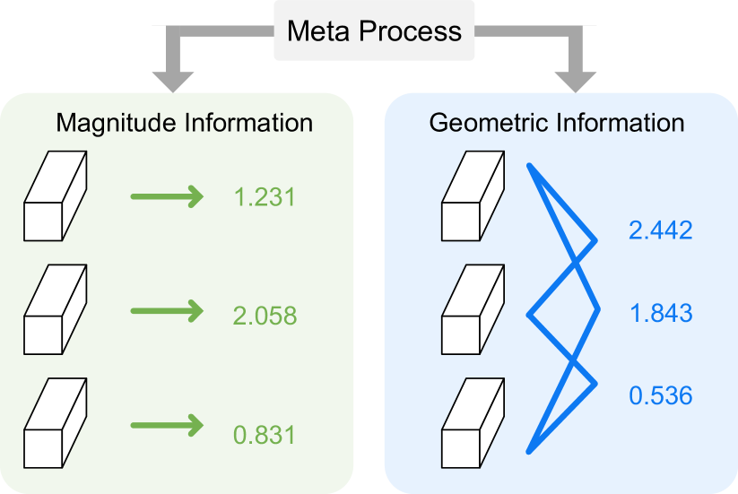
Figure 1: The meta-process selects suitable information for pruning. Magnitude information depends on the filter itself, while geometric information is based on two filters.

Recently, pruning filters in a soft manner [13, 14, 15, 16, 17, 18] have proven to be more effective than the conventional three-stage pipeline. The advantage of soft filter pruning is that previously pruned filters can be updated during training. Once the training process is complete, the removal of unimportant filters from the network can take place. In this way, the model’s capacity will not decrease, and network performance is enhanced.

However, previous works using the soft filter pruning have two drawbacks. First, previous filter pruning works often ignore the geometric information between filters when pruning. Prevailing filter pruning works [11, 19, 14] are based on the “smaller-norm-less-important” criterion. The basis of this criterion is that filters with smaller norms are less critical, and therefore, pruning those filters with smaller $\ell_{1}$-norm [11] or $\ell_{2}$-norm [14] will not bring dramatic performance drop. Although the $\ell_{p}$-norm-based criterion focuses on the magnitude information of individual filters, the criterion ignores the geometric information between filters; a disadvantage that may lead to inappropriate pruning results. Research by [20] show that the filters in the network have regular patterns, thus considering the geometric information is critical for pruning. Here is an example, suppose we have three filters to prune, each of which is a three-dimension vector: $A=(1,1,1)$, $B=(1.1,1,1)$, and $C=(0.5,0.3,0.2)$. Norm-based criterion would prune $C$ since it has the smallest norm. However, if we look closely at $A$ and $B$, we will find that they are statistically similar. Therefore, they make a very similar, if not the same, contribution to the network, which means pruning either $A$ or $B$ is more reasonable. We need to be careful when the value of a filter becomes zero. Filter $C$ will become zero only when the filter is pruned. Under this condition, filter $C$ should remain zero since the pruned filters should not change to a non-zero value. Second, in previous works [13, 14, 15, 16, 17, 18], the weights of the network are updated to new values after pruning and training. However, the pruning criterion during the entire training and pruning process keeps fixed and fails to adapt to current conditions. A fixed criterion may not be able to evaluate a network of different weight values. For the first problem, we introduce new measures to rank filters, using their geometric information. Assume a filter space contains all the filters of the network, different weights values indicate that the filters are located in various positions of the filter space. In this way, we could utilize the distance between the filters to characterize the geometric information among filters. Specifically, Minkowski distance, an effective similarity measure [21], is employed to measure the geometric information. After we obtain the geometric information of filters, we can prune the filters that make a replaceable contribution to the network. To solve the second problem, we build a Meta-attribute-based Filter Pruning (MFP) framework to adaptively select the most appropriate criteria based on the current state of the network. As shown in Fig. 1, during pruning and training, networks with different values would have various meta-attributes [22]. These meta-attributes are particularly effective in measuring the difference between the networks and assist in choosing the optimally pruned one from the candidates. Inspired by the meta-learning framework [22], we minimize the meta-attributes of the pruned model and the original model, which enables the pruned models to perform as well as the original models on the pre-defined task.

Contributions. We outline three contributions:

(1) We introduce distance-based measures to model the geometric information among the filters, which is complementary to the existing magnitude measures.

(2) We utilize the meta-attribute to characterize the difference between pruned and original models. Following a meta-learning way, we adaptively select a suitable meta-attribute based on the current network state and conduct pruning based on the selected meta-attribute.

(3) The experiments on two benchmarks validate the effectiveness of our MFP. For ResNet-50 on ILSVRC-2012, we could reduce more than 50% FLOPs with only 0.44% top-5 accuracy loss. Moreover, our MFP accelerates ResNet-110 on CIFAR-10 by two times with even 0.16% relative accuracy improvement.

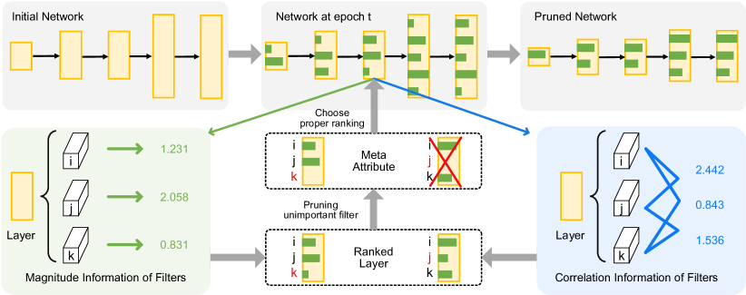
Figure 2: The process of our pruning method. Filters of a layer would be ranked based on the magnitude and the geometric information. Then the meta-attribute of the network is utilized to determine which information should be used for pruning at the current state.

II Related Work

Based on the granularity of pruning, network pruning can be divided into weight pruning [9, 23, 13, 24, 10, 25, 26] and filter pruning [11]. The former one focuses on pruning the fine-grained weight of filters, but the unstructured sparsity in the pruned model makes it less friendly for realistic acceleration. On the other hand, filter pruning achieves structured sparsity and a realistic acceleration with high-efficiency Basic Linear Algebra Subprograms (BLAS) libraries.

II-A Weight Pruning.

Many recent works [9, 23, 13] prune weights of the neural network to produce small models. For example, [9] proposes an iterative weight pruning method by discarding the small weights with values below the threshold. Dynamic network surgery is employed by [13] to reduce the training iteration while maintaining good prediction accuracy. [27, 28] leverage the sparsity property of feature maps or weight parameters to accelerate the CNN models. A special case of weight pruning is known as neuron pruning. [29] evaluates the importance of neurons by measuring the sparsity of ReLU activations. However, pruning weights always leads to unstructured models, so the model cannot leverage the existing efficient BLAS libraries in practice. Therefore, it is difficult for weight pruning to achieve a realistic speedup.

II-B Filter Pruning.

If we consider whether to utilize the training data to determine the pruned filters, we could further divide the filter pruning methods into two categories:

Training Data Dependent Filter Pruning.  [30, 31, 32, 33, 34, 35, 12, 36, 37, 38, 39, 40, 41, 42, 43, 44, 40, 45] utilize the training data to determine the pruned filters. [39] leverages the reinforcement learning to find the redundancy for each layer automatically. Sparsity regularization on the scaling factors of the network is imposed by [30]. He et al. [32] utilizes the LASSO regression to select channels. Yu et al. [12] proposes to minimize the reconstruction error of important responses in the “final response layer”, and derives a closed-form solution to prune neurons in earlier layers. Kang et al. [46] proposes data-driven SCP algorithm to prune models in a differentiable way. Gao et al. [47] considers the loss-metric mismatch problem and uses NPPM to solve the problem in pruning. DSA [48] finds the layer-wise pruning ratios with gradient-based optimization.

Training Data Independent Filter Pruning. Some training data-independent filter pruning methods [11, 14, 19, 49, 50, 51, 52, 53, 54, 55] have been proposed. [11] and [14] prune the filters with the $\ell_{1}$-norm criterion and $\ell_{2}$-norm criterion, respectively. Research by [56] claims that the filters near the geometric median should be pruned, [19] proposes to prune the network by introducing sparsity on the scaling parameters of batch normalization (BN) layers, and [49] clusters the filters in the spectral domain to select the unimportant filters. CLR [57] finds a better learning rate schedule for pruning.

Some previous work [58, 26, 38, 59, 60] use the “meta” word or a similar term such as “learning to prune”, but the core idea is different from our proposed mete-attribute-based filter pruning method. [58] focuses on modeling the complex software systems at high-levels of abstraction, rather than the neural network. In this situation, pruning refers to the removal of unnecessary classes and properties of software systems, not filters of the neural network. [26] conducts pruning based on second-order derivatives of a layer-wise error function. The “learning” word means second order derivatives. Moreover, [38] utilizes a reinforcement learning framework to determine the pruning filters.  [60] generates the weights of the pruned network by a proposed PruningNet. To the best of our knowledge, none of the previous works mentions the meta-attributes for measuring the similarity of the original model and pruned model.

Some of the previous works [61] utilize the correlation for filter pruning, but there are some differences between their work and ours. First, [61] needs to calculate the pair-wise node-correlation first before calculating the filter correlation. In contrast, our approach does not need extra node-correlation since we can directly calculate the distance between filters. Second, [61] adopts normalized correlation-based importance to measure the redundancy between two filters, while we use the Minkowski distance as a measure to include the filter scale. Third, [61] contains two regularization terms in the final importance, which would introduce extra hyper-parameters. In contrast, our method does not rely on any regularization term since the filter distance can be used as the filter importance in a direct manner.

The differences between Imp [62] and our method include: 1) Different importance measure methods: Imp [62] use Hessian matrix, while we use magnitude information and correlation information of filters. 2) Different dependence of dataset: Imp [62] needs a few batches of input data to choose the filters, but we rely only on the weight values of the filters. 3) Different ways to select models: Imp [62] utilizes importance score accumulation to select neurons, but we use meta-attributes to choose the pruned models.

II-C Neural Architecture Search

Some previous works use Neural Architecture Search (NAS) to automatically obtain the neural networks. There are several differences between NAS and pruning. 1) Different objectives: NAS aims at obtaining new networks automatically, while pruning focus on compressing and accelerating the existing models to achieve higher performance. 2) Different components: NAS usually has many different kinds of cells as the searching components, while pruning methods consider the convolutional layers as the basic components. 3) Different computations are required. Due to the large search space, NAS usually requires much more computational resources than pruning. While our method only costs several GPU days or even several GPU hours. DARTS [63] proposes to search the architecture automatically using cells including separable convolutions, dilated separable convolutions, max pooling. EfficientNet [64] searches the depth, width, and resolution of the network with mobile inverted bottleneck MBConv. NASNet [65] requires 2000 GPU days for searching the architectures.

III Meta Filter Pruning

III-A Preliminaries

First, we assume that a neural network has $L$ layers and the number of input and output channels in $i_{th}$ convolution layer is $N_{i}$ and $N_{i+1}$, respectively. Suppose $K$ is the kernel size of the layer, we use $\mathcal{F}_{i,j}$ to represent the $j_{th}$ filter in the $i_{th}$ layer, and $\mathcal{F}_{i,j}\in\mathbb{R}^{N_{i}\times K\times K}$. For the $i_{th}$ layer, it consists of a set of filters denoted by $\{\mathcal{F}_{i,j},1\leq j\leq N_{i+1}\}$ and parameterized by $\{\mathbf{W}^{(i)}\in\mathbb{R}^{N_{i+1}\times N_{i}\times K\times K},1\leq i\leq L\}$.

For the convenience of our discussion, we assume $\mathcal{F}_{i,j}$ consists of two subsets: the pruned filter set ${\mathcal{F}}^{pruned}$, and the remaining filter set ${\mathcal{F}}^{keep}$. Specifically:

$${\mathcal{F}}^{keep} =\big{\{}{\mathcal{F}}_{i,j},\quad for\enspace i\in[1,L],\enspace j\in ID(i)\enspace\big{\}}$$ (1)

where $ID(i)$ is the index of important filters in layer $i$.

Given a dataset ${\mathcal{D}}=\{({\mathbf{x}}_{i},{\mathbf{y}}_{i})\}_{i=1}^{n}$, and a desired sparsity level $\kappa$ (i.e., the number of remaining non-zero filters), we solve a constrained optimization problem, defined as follows:

$$\min_{{\mathcal{F}}^{keep}}\ell({\mathcal{F}}^{keep};{\mathcal{D}}) =\min_{{\mathcal{F}}^{keep}}\frac{1}{n}\sum_{i=1}^{n}\ell({\mathcal{F}}^{keep};({\mathbf{x}}_{i},{\mathbf{y}}_{i}))$$ (2)

$$\text{s.t.}\quad N_{set}({\mathcal{F}}^{keep}) \leq\kappa,\quad{\mathcal{F}}\in\mathbb{R}^{N\times K\times K}.$$

where $\ell(\cdot)$ is a standard loss function (e.g., cross-entropy loss), ${\mathcal{F}}^{keep}$ is the set of remaining filters of the neural network, and $N_{set}$ is the cardinality of the filter set.

III-B Information From the Filters

For filter pruning, the most critical part is to evaluate the importance of the filters. For filters with specific weight values, we could obtain the magnitude information and the geometric information of the filters.

III-B1 Magnitude Information

Magnitude-based criterion believes that the convolutional results of the filter with the smaller $\ell_{p}$-norm lead to relatively lower activation values [11], so the contribution of the small-norm filters to the final prediction of deep CNN models is less than that of large-norm filters. The $\ell_{p}$-norm of filters is:

$$\|\mathcal{F}_{i,j}\|_{p}=\sqrt[p]{\sum_{n=1}^{N_{i}}\sum_{k_{1}=1}^{K}\sum_{k_{2}=1}^{K}\left|\mathcal{F}_{i,j}(n,k_{1},k_{2})\right|^{p}}$$ (3)

In terms of this understanding, we give a high priority to prune the filters of a small $\ell_{p}$-norm than filters of a higher $\ell_{p}$-norm, which could be formulated as:

$$j^{*}=\operatorname*{arg\,min}_{j\in[1,N_{i+1}]}\|\mathcal{F}_{i,j}\|_{p},$$ (4)

III-B2 Geometric Information

As the $\ell_{p}$-norm only models the magnitude information of the filters, we introduce the distance of filters to reflect the geometric information between them. We utilize the Minkowski distance [21] as our selection. For simplicity, we reshape or extend the three-dimensional filter $\mathcal{F}_{i,j}$ to one-dimensional vector. Then, the $i_{th}$ convolution layer could be written as ${\mathcal{Y}}\in\mathbb{R}^{N_{i+1}\times G_{i}}$, which means $N_{i+1}$ vectors and the length of each vector is $G_{i}=N_{i}\times K\times K$. If we choose two vectors $\boldsymbol{x},\boldsymbol{y}\in\mathbb{R}^{1\times G_{i}}$. Then the Minkowski distance between $\boldsymbol{x}$ and $\boldsymbol{y}$ is:

$$D(\boldsymbol{x},\boldsymbol{y})=\sqrt[q]{\sum_{i=1}^{G_{i}}\left|x_{i}-y_{i}\right|^{q}},$$ (5)

where $x_{i}$ is the $i_{th}$ element of the vector $\boldsymbol{x}$.

Note that Minkowski distance is a general distance which can be considered as a generalization of both the Manhattan distance [66] and the Euclidean distance [67]. Therefore, it is easy to cover different kinds of distance by adjusting the value of the parameter $q$ in Eq. 5. That is to say, it is simple for us to increase the candidate filter importance measurement methods, thus enlarging our search space. For example, if we use $q=1$ in Eq. 5, we get the Manhattan distance. If we use $q=2$ in Eq. 5, we obtain the Euclidean distance.

For simplicity, we discuss pruning only one filter of a network layer with $N$ filters. To reduce the accuracy gap between the pruned model and the original model, the remaining $N-1$ filter should best approximate the original $N$ filters. In other words, the contribution of this pruned filter should be replaced by the remaining $N-1$ filters. Based on this consideration, we prefer to remove the filter that minimizes the average distance to other filters. To this end, we define the average distance for a filter as the importance evaluation, which could be formulated as:

$$D_{avg}({{\mathcal{Y}}_{p}})=\frac{\sum_{p=1,p\neq q}^{N_{i+1}}D({\mathcal{Y}}_{p},{\mathcal{Y}}_{q})}{N_{i+1}}=\frac{\sum_{p=1}^{N_{i+1}}D({\mathcal{Y}}_{p},{\mathcal{Y}}_{q})}{N_{i+1}},$$ (6)

where ${\mathcal{Y}}_{p}$ is the $p_{th}$ filter vector of the layer. So the index of the pruned filter could be formulated as:

$$p^{*}=\operatorname*{arg\,min}_{p\in[1,N_{i+1}]}D_{avg}({{\mathcal{Y}}_{p}}).$$ (7)

III-C Meta-attribute based Pruning

Depth	Method	Pre-train?	Baseline acc. (%)	Accelerated acc. (%)	Acc. $\downarrow$ (%)	FLOPs	FLOPs $\downarrow$(%)
32	MIL [68]	✗	92.33	90.74	1.59	4.70E7	31.2
	Ours (40%)	✗	92.63 ($\pm$0.70)	91.85 ($\pm$0.09)	0.78	3.23E7	53.2
56	PFEC [11]	✗	93.04	91.31	1.75	9.09E7	27.6
	CP [32]	✗	92.80	90.90	1.90	–	50.0
	SFP [14]	✗	93.59 ($\pm$0.58)	92.26 ($\pm$0.31)	1.33	5.94E7	52.6
	Ours (40%)	✗	93.59 ($\pm$0.58)	92.76 ($\pm$0.03)	0.83	5.94E7	52.6
2-8	PFEC [11]	✓	93.04	93.06	-0.02	9.09E7	27.6
	DSA [48]	✓	93.12	92.91	0.22	–	49.7
	CP [32]	✓	92.80	91.80	1.00	–	50.0
	AMC [69]	✓	92.80	91.90	0.90	–	50.0
	NPPM [47]	✓	93.59 ($\pm$0.58)	93.40 ($\pm$0.34)	0.19	–	50.0
	SCP [46]	✓	93.59 ($\pm$0.58)	93.23	0.36	–	51.5
	FPGM [56]	✓	93.59 ($\pm$0.58)	93.26 ($\pm$0.03)	0.33	5.94E7	52.6
	CLR [57]	✓	93.59 ($\pm$0.58)	92.78 ($\pm$0.34)	0.81	5.94E7	52.6
	Ours (40%)	✓	93.59 ($\pm$0.58)	93.56 ($\pm$0.16)	0.03	5.94E7	52.6
110	PFEC [11]	✗	93.53	92.94	0.61	1.55E8	38.6
	MIL [68]	✗	93.63	93.44	0.19	-	34.2
	SFP [14]	✗	93.68 ($\pm$0.32)	93.38 ($\pm$0.30)	0.30	1.50E8	40.8
	Rethink [70]	✗	93.77 ($\pm$0.23)	93.70 ($\pm$0.16)	0.07	1.50E8	40.8
	Ours (40%)	✗	93.68 ($\pm$0.32)	93.69 ($\pm$0.31)	-0.01	1.21E8	52.3
	Ours (50%)	✗	93.68 ($\pm$0.32)	93.38 ($\pm$0.16)	0.30	9.40E7	62.8
2-8	PFEC [11]	✓	93.53	93.30	0.20	1.55E8	38.6
	NISP [12]	✓	–	–	0.18	–	43.8
	CLR [57]	✓	93.68 ($\pm$0.32)	92.91 ($\pm$0.41)	0.77	1.21E8	52.3
	Ours (40%)	✓	93.68 ($\pm$0.32)	93.31 ($\pm$0.08)	0.37	1.21E8	52.3

TABLE I: Comparison of the pruned ResNet on CIFAR-10. In “Pre-train?” column, “✓” and “✗” indicate pruning the pre-trained and scratch model, respectively. The “Acc. $\downarrow$” is the accuracy drop between the pruned model.

Existing works [11, 14] prune the filters based on a pre-defined criterion, without considering the change of filter distribution due to network weights updating. In this section, we illustrate our proposed meta-attribute based pruning method, which can adaptively choose an appropriate criterion based on the current state of the network.

As shown in [22], the general, statistical and information theoretic measures to characterize the datasets are called meta-attributes of the datasets. In the filter pruning scenario, we should minimize the difference of the meta-attributes in the original network (${\mathcal{F}}$) and those in the pruned network (${\mathcal{F}}^{keep}$). If the meta-attributes of these two networks are similar, ${\mathcal{F}}^{keep}$ could achieve performance as good as ${\mathcal{F}}$ do.

Previous works provided by [32, 14] combine the pruning process and training process, then conduct pruning in an iterative manner. We follow them and model the meta-process of filter pruning as a sequential decision process in a greedy approach. The entire pruning and training process is illustrated in Fig. 2, which is elaborated as follows.

• Assume $S$ is a set of states. In our case, $s_{t}\in S$ is the network at the $t_{th}$ training epochs. At each time step $t$, $s_{t}$ is available to the meta-process which decides the remaining filter set ${\mathcal{F}}^{keep}_{t}$.

• At the $t$-th step, given the state $s_{t}$, the meta-process takes an action to choose the proper pruning criteria for filter importance evaluation. We use $\mathcal{A}_{t}$ to indicate the action of the $t$-th step. Assume we have $C$ candidate pruning criteria, then $\mathcal{A}_{t}\in\mathbb{R}^{C\times 1}$. For each dimension of $\mathcal{A}_{t}$, we use the binary value 0,1 to indicate whether a specific pruning criterion is selected (1 means selected, and 0 means not selected). In our setting, only one pruning criterion is chosen for the current state, which is:

  $$\sum_{i=1}^{C}\mathcal{A}_{t,i}=1,\quad\mathcal{A}_{t,i}\in\{0,1\},$$ (8)

  where $\mathcal{A}_{t,i}$ means the indicator of the $i_{th}$ criteria in the $t_{th}$ step.

• $\phi:S\rightarrow\mathcal{A}$ is the policy employed by the meta-process to generate its action: $\phi(s_{t})=\mathcal{A}_{t}$. For filter pruning, the policy should aim at reducing the difference between meta-attributes of the pruned models and the original models:

  $$\mathcal{A}_{t}^{*}=\operatorname*{arg\,min}_{\mathcal{A}_{t}}{\mid{\mathbf{M}}(\mathcal{F}_{\mathcal{A}_{t}})-{\mathbf{M}}(\mathcal{F})\mid},$$ (9)

  where ${\mathbf{M}}$ represents the meta-attributes of the network, $\mathcal{F}_{\mathcal{A}_{t}}$ is the pruned network under a specific criterion from the action $\mathcal{A}_{t}$. Several measures could be utilized as meta-attributes, such as sparsity level $\kappa$, the mean value of weights, top-5 loss, top-1 loss, and so on.

• After we enter time step $t+1$, we follow the above protocol and take action $a_{t+1}$ based on the state $s_{t+1}$.

Algorithm 1 Algorithm Description of MFP

1:training data: $\mathbf{X}$, model $\mathbf{W}=\{\mathbf{W}^{(i)},0\leq i\leq L\}$.

2:Given: pruning rate $P_{i}$

3:Initialize: model parameter $\mathbf{W}$

4:for $epoch=1$; $epoch\leq epoch_{max}$; $epoch++$ do

5:     Update the model parameter $\mathbf{W}$ based on $\mathbf{X}$

6:     Find $\mathcal{A}^{*}$ that satisfy Eq. 9

7:     for $i=1$; $i\leq L$; $i++$ do

8:         Using $\mathcal{A}^{*}$ to prune $N_{i+1}P_{i}$ filters

9:     end for

10:end for

11:Obtain the compact model $\mathbf{W}^{*}$ from $\mathbf{W}$

12:The compact model and its parameters $\mathbf{W}^{*}$

The algorithm of meta filter pruning is shown in Algorithm 1. Although there are a few similarities between our algorithm and evolving Takagi–Sugeno (TS) fuzzy model [71], there are still significant differences between them. Specifically, a TS model defines neighboring models as a certain number of models with split and merge operations. Then the TS model switches to one of the neighboring models at each stage of evolving. In contrast, our method treats models with different meta-attributes as neighboring models, and we select one of those models during our training process. We zeroize the selected filters to maintain the model capacity of the network [14], but the process has the same effect as pruning [11].

III-D Scope of Search

III-D1 Reasonable Filter Ranking Criteria

If we define the search scope by directly selecting a number of filters, the search scope is surprisingly large for those frequently used CNN architectures. For example, if we want to keep $n$ filters in $i_{th}$ layer, which has a total of $N_{i+1}$ filters, then the number of selections would be $\dbinom{N_{i+1}}{n}=\frac{N_{i+1}!}{n!\enspace(N_{i+1}-n)!}$, where $\dbinom{}{}$ denotes the combination [72]. We take ResNet-50 for example. The first layer of ResNet-50 has 64 filters and the total number of selecting 10 filters is $\dbinom{64}{10}=151,473,214,816$ selections. The upper layers with more filters would have a much higher selection number. As a result, the number of the candidate neighboring CNNs is very large and the computational cost is not affordable if we conduct brute-force searching.

Considering the above, adapting the filter ranking criteria is necessary to reduce the searching space. In this way, the scope of search is mainly decided by the number of reasonable filter ranking criteria. Suppose we have $S$ filter ranking criteria, the number of selecting $n$ filters from $N_{i+1}$ filters would decrease from $\dbinom{N_{i+1}}{n}$ to $S$, which is a reasonable size of the search space.

III-D2 Clear Model Judgment

Another factor we need to consider is that the model judgment should be conducted clearly. Suppose the number of candidate acceleration ratios for pruned models is $R$. For every acceleration ratio, the number of neighboring CNNs is $S$ considering the number of criteria is $S$. So the total number of candidate CNNs is $R\times S$.

We consider two aspects to judge the performance of a model, i.e., accuracy and acceleration ratio (FLOPs). It is difficult to evaluate since those two aspects are contradictory to each other. For example, suppose a model has a 10% acceleration ratio with a 1% accuracy drop, and another model has a 20% acceleration ratio with a 2% accuracy drop. In this situation, it may be difficult to choose between the two models. To solve this problem, we fix one of the two aspects, i.e., acceleration ratio, and utilize the accuracies under the same acceleration ratio to judge the model performance. In this way, the total number of candidate CNNs for a specific acceleration ratio is $S$.

III-E Acceleration Analysis

In the above analysis, the ratio of pruned FLOPs is $1-(1-P_{i+1})\times(1-P_{i})$ theoretically. As other operations such as batch normalization (BN) and pooling are insignificant compared to convolution operations, it is common to utilize the FLOPs of convolution operations as the FLOPs of the network [11, 14].

However, in the real scenario, non-tensor layers (e.g., pooling and BN layers) also need the computation time on GPU [31] and the realistic acceleration may be influenced. Besides, other factors such as buffer switch, IO delay and the efficiency of BLAS libraries also lead to the gap between the realistic and theoretical acceleration. We compare the different acceleration ratios in Table IV.

IV Experiments

Depth	Method	Pre- train?	Baseline top-1 acc.(%)	Accelerated top-1 acc.(%)	Baseline top-5 acc.(%)	Accelerated top-5 acc.(%)	Top-1 acc. $\downarrow$(%)	Top-5 acc. $\downarrow$(%)	FLOPs$\downarrow$ (%)
18	MIL [68]	✗	69.98	66.33	89.24	86.94	3.65	2.30	34.6
	SFP [14]	✗	70.28	67.10	89.63	87.78	3.18	1.85	41.8
	Ours (30%)	✗	70.28	67.66	89.63	87.90	2.62	1.73	41.8
2-10	Ours (30%)	✓	70.28	68.31	89.63	88.28	1.97	1.35	41.8
	COP [61]	✗	70.29	66.98	–	–	3.31	–	43.3
	Ours (40%)	✓	70.28	67.11	89.63	87.49	3.17	2.14	51.8
50	Ours (40%)	✗	76.15	74.13	92.87	91.94	2.02	0.93	53.5
2-10	Imp [62]	✓	76.18	74.48	–	–	1.70	–	35.0
	ThiNet [31]	✓	72.88	72.04	91.14	90.67	0.84	0.47	36.7
	SFP [14]	✓	76.15	62.14	92.87	84.60	14.01	8.27	41.8
	CLR [57]	✓	76.15	75.26	–	–	0.89	–	43.0
	NISP [12]	✓	–	–	–	–	0.89	–	44.0
	CP [32]	✓	–	–	92.20	90.80	–	1.40	50.0
	LFC [73]	✓	75.30	73.40	92.20	91.40	1.90	0.80	50.0
	ELR [36]	✓	–	–	92.20	91.20	–	1.00	50.0
	DSA [48]	✓	–	–	–	–	1.33	–	50.0
	Meta [60]	✓	76.60	75.40	–	–	1.20	–	51.2
	Ours (30%)	✓	76.15	75.67	92.87	92.81	0.48	0.06	42.2
	Ours (40%)	✓	76.15	74.86	92.87	92.43	1.29	0.44	53.5

TABLE II: Comparison of the pruned ResNet on ImageNet. “Pre-train?” and ”acc. $\downarrow$” have the same meaning with Table I.

IV-A Dataset and Architecture

The experiments are conducted on two benchmark datasets, CIFAR-10 [74] and ILSVRC-2012 [75]. The CIFAR-10 dataset contains a total of $60,000$ images, which contains $50,000$ training images and $10,000$ testing images in $10$ different classes. ILSVRC-2012 [75] contains 1.28 million training images and 50k validation images of $1,000$ classes.

We focus on pruning the challenging multi-branch ResNet model [68, 31, 32]. Moreover, to validate our method on the single-branch network, we follow [11] to conduct a test on the VGGNet [76].

IV-B Training and Pruning

Training Setting. For VGGNet on CIFAR-10, we follow the setting in [11]. As the training setup is not publicly available, we re-implement the pruning procedure and achieve similar results to the original paper. For ResNet on CIFAR-10, we utilize the same training schedule as [77]. For CIFAR-10 experiments, we run each setting three times and report the “mean $\pm$ std”. In the ILSVRC-2012 experiments, we use the default parameter setting, which is the same as [8, 78], and the same data argumentation strategies as the official PyTorch [79] examples.

Pruning Setting. For VGGNet on CIFAR-10, we use the same pruning rate as [11]. For experiments on ResNet, we follow [56, 14] and prune all the weighted layers with the same pruning rate at the same time. Therefore, only one hyper-parameter, the pruning rate of $P_{i}=P$ is used to balance the acceleration and accuracy. Note that choosing different rates for different layers could improve the performance [11], but it also introduces extra hyper-parameters. Our pruning operation is conducted at the end of every two training epochs, which provides a balance of accuracy and energy consumption during the pruning operation. Pruning of both the scratch model and the pre-trained model are compared. For pruning from scratch, we train the model from scratch and do not conduct additional fine-tuning. For pruning the pre-trained model, the learning rate is reduced to one-tenth of the initial learning rate. The training schedule is the same as [14].

Meta-Process Setting. The execution time would increase when the number of neighboring CNN increases. Specifically, the total execution time contains two parts. First, the time for the network training process. Second, the time for search at the end of the training epoch. Increasing the number of neighboring CNNs would affect the second part of the execution time, but not on the first part. For example, on the Quadro RTX 6000 GPU, training CIFAR-10 for one epoch takes 27.7 seconds, while searching for $N$ pruned models takes about $N\times 6.9$ seconds. To ensure the searching time does not exceed the training time too much, the value of $N$ is 4. So we follow the definition of the scope of search in Section III.D and choose to search four pruned models. These models are obtained from four pruning criteria, including $p=1,2$ in Eq. 3 for magnitude information, which are $\ell_{1}$-norm criteria [11] and $\ell_{2}$-norm criteria [14], respectively, and $q=1,2$. in Eq. 5 for geometric information, which are Manhattan distance and the Euclidean distance, respectively. Note that our framework is compatible with any new pruning criterion. Based on the result in Sec. IV-F, we consider the top-5 loss as the meta-attributes to evaluate the network at the current state. Besides, the sparsity level $\kappa$ is utilized as a meta-attribute to balance the accuracy and the computational cost.

In Table I and Table II, the method labeled “Ours (40%)” means we prune 40% filters of the layers during training when the pruned filters is recovered. We compare our method with existing state-of-the-art acceleration algorithms, e.g., MIL [68], PFEC [11], CP [32], ThiNet [31], SFP [14], NISP [12], FPGM [56], LFC [73], ELR [36], AMC [69], DSA [48], NPPM [47], SCP [46], CLR [57]. Experiments show that our MFP achieves the comparable performance with the state-of-the-art results.

IV-C VGGNet on CIFAR-10

The result of pruning scratch and pre-trained VGGNet is shown in Table III. Not surprisingly, MFP achieves better performance than [11] in both settings. With the pruning criterion selected by our method, we could achieve better accuracy than [11] when pruning the random initialized VGGNet (93.54% v.s.93.31%). In addition, the pruned model without fine-tuning has better performance than [11] (84.80% v.s.77.45%). After fine-tuning $40$ epochs, our model achieves similar accuracy with [11]. Notably, if more fine-tuning epochs ($160$) are used, [11] achieve similar result with fine-tuning $40$ epochs (93.28% v.s.93.22%), while our method could attain a much better performance (93.76% v.s.93.26%).

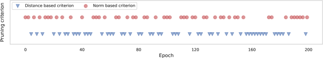
(a) Initialization 1

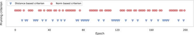
(b) Initialization 2

Figure 3: Learned pruning criterion during the training process of ResNet-110 on CIFAR-10 under different initializations. The pruning rate is 40%. The red and blue marker denotes the norm-based criterion and the distance-based criterion, respectively.

Setting $\backslash$ Acc (%)	PFEC [11]	Ours
Baseline	93.58 ($\pm$0.03)	93.58 ($\pm$0.03)
Prune from scratch	93.31 ($\pm$0.03)	93.54 ($\pm$0.03)
Prune pretrain w.o. FT	77.45 ($\pm$0.03)	84.80 ($\pm$0.03)
FT 40 epochs	93.22 ($\pm$0.03)	93.26 ($\pm$0.03)
FT 160 epochs	93.28 ($\pm$0.03)	93.76 ($\pm$0.08)

TABLE III: Pruning scratch and pre-trained VGGNet on CIFAR-10. The abbreviation “w.o. FT” means “without fine-tuning”.

IV-D ResNet on CIFAR-10

For the CIFAR-10 dataset, we test our MFP on ResNet (depth $32$, $56$ and $110$). We use two different pruning rates 40% and 50%. As shown in Table I, the experiment results validate the effectiveness of our method.

Result Explanation. For example, comparing to SFP [14], when we prune 52.6% FLOPs of the scratch ResNet-56, our MFP has a 0.50% accuracy improvement over SFP [14] (0.83% v.s.1.33%). Besides, MIL [68] accelerates the scratch ResNet-32 by a 31.2% speedup ratio with a 1.59% accuracy drop, but our MFP achieves a higher speedup ratio with only less accuracy drop. For pruning the pre-trained ResNet-56, our method achieves a higher acceleration ratio than CP [32] with a 0.97% accuracy increase over CP [32]. When compared with PFEC [11], our method achieves a higher speedup ratio even with accuracy improvement. Comparing to DSA [48], we achieve the 2.9% more acceleration ratio with 0.19% less accuracy drop on ResNet-56. When we achieve the same speed-up ratio with CLR [57], our accuracy is 0.74% better than CLR [57] on ResNet-56. Our performance is also better than NPPM [47] and SCP [46] in terms of both accuracy and acceleration ratio. Moreover, we achieve a better accuracy than [70], which is consistent with the conclusion by [70] that different initializations would lead to different result networks. The first reason for our superior result is that our criterion explicitly models the geometric information between filters by taking advantage of three corresponding measures. Besides, we adaptively select the suitable criteria to match the current filter distribution, which may keep changing during the pruning process. Previous works [68, 14, 32, 11, 12] pre-specify a criterion before pruning and keep it fixed during the entire pruning process, yet fail to consider that the selected criterion may no longer be suitable any more after epochs of training.

(a) Accuracy of ResNet-110 on CIFAR-10 with different FLOPs.

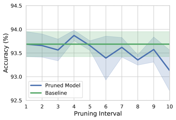
(b) Accuracy of ResNet-110 on CIFAR-10 with various pruning intervals.

Figure 4: Accuracy of ResNet-110 on CIFAR-10 regarding different FLOPs and pruning interval.

IV-E ResNet on ILSVRC-2012

For the ILSVRC-2012 dataset, we test our method on ResNet-18 and ResNet-50; and we use pruning rate 30% and 40% for these models. Following [14], we do not prune the projection shortcuts. The results are shown in Table II.

Result Explanation. For the random initialized ResNet-18, MIL [68] accelerates the network by a 34.6% speedup ratio with a 3.65% accuracy drop, but our MFP achieves a 41.8% speedup ratio (7.20% better) with only a 2.62% accuracy drop (1.03% better). Comparing to SFP [14], when we prune the same ratio (41.8%) of FLOPs of the ResNet-18, our MFP has a 0.56% accuracy improvement over SFP [14].

For pruning the pre-trained ResNet-50, our MFP reduces 41.8% FLOPs in the network with only a 0.06% top-5 accuracy drop. In contrast, ThiNet [31] reduces 36.7% FLOPs (5.1% worse than ours) with a 0.47% top-5 accuracy drop (0.41% worse than ours). In addition, SFP achieves the same acceleration ratio as MFP, with a 8.27% top-5 accuracy drop (8.21% worse than ours). Comparing to NISP [12], we achieve a similar acceleration ratio with a smaller accuracy drop (0.48% v.s. 0.89%). When we prune 53.5% FLOPs of the pre-trained ResNet-50, our MFP has 0.44% top-5 accuracy drop, while CP [32] reduces 50.0% FLOPs of the network with 1.40% top-5 accuracy (0.96% worse than ours). Comparing to Imp [62], we achieve a 18.5% more acceleration ratio (53.5% v.s. 35.0%) with a 0.41% smaller accuracy drop (1.29% v.s. 1.70%). When we achieve a similar FLOPs drop rate with COP [61], our accuracy drop is 1.34% less than COP [61]. Also, We can obtain 8.5% more acceleration ratio with 0.14% less accuracy drop than COP [61]. We also achieve comparable results with MetaPruning [60], when our speed-up ratio is 2.3% better than MetaPruning [60] (53.5% v.s. 51.2%), the accuracy drop is similar (1.29% v.s. 1.20%). The superior performance may come from that our method consider the magnitude information and the geometric information of the filters.

IV-F Case Study

Figure 5: Input image (left) and visualization of feature maps (right, numbered 0 to 63). Selected channels are pruned with norm-based criterion and relation-based criterion. The feature maps are extracted from the first convolutional layer of the first block of ResNet-18. The pruning rate is 10%. Feature maps with a black title and box (channel 29, 44, 51, 56) denote the common channels selected by both criteria. Feature maps with a red title and box (30, 62) denote the channels only selected by norm-based criterion, while feature maps with an orange title and box (24, 52) denote the channels only selected by distance-based criterion.

Different Criteria During Training. The pruning criterion during the training process of two different initializations are shown in Fig. 3. The norm-based criterion includes 1-norm and 2-norm. The relational criterion includes Manhattan distance and Euclidean distance. By comparing these two figures, we conclude that our MFP could adaptively select proper criteria during the training process with different initializations. For the selected pruning criteria, we find that during the early training process, the distance-based criteria are adopted less than norm-based criteria. The above phenomena may be caused by the training knowledge from the training set. During the early training stage, the filters have not learned enough training set knowledge, and the geometric information of filters is not particularly meaningful, so the norm-based criteria are preferred. After more training epochs, the filters obtain the information from the training set, and the geometric information of filters becomes meaningful; then the distance-based criteria begins to take effect.

Realistic Acceleration. We measure the forward time of the pruned models to compare the theoretical and realistic acceleration. The experiment is conducted on one GTX1080 GPU with a batch size of 64 (Table IV). As discussed in the above section, the gap between the theoretical and the realistic acceleration may come from the limitation of IO delay, buffer switch and efficiency of BLAS libraries.

Memory Footprint. We test the memory footprint before and after pruning on NVIDIA RTX6000 GPU. For a batch size of 256, ResNet on CIFAR-10 requires 1423MB memory footprint before pruning. After pruning 52.3% FLOPS, the required memory footprint is 840MB, which is 41.0% less than the original memory footprint. The gap comes from operations such as batch normalization (BN) and pooling.

Model	Baseline time (ms)	Pruned time (ms)	Realistic Speedup(%)	Theoretical Speedup(%)
ResNet-18	37.50	26.17	30.2	41.8
ResNet-50	136.24	84.33	38.1	53.5

TABLE IV: Comparison of the theoretical and realistic acceleration. Only the time consumption of the forward procedure is considered.

Varying Pruned FLOPs. We change the ratio of pruned FLOPs for ResNet-110 on CIFAR-10 to comprehensively understand our MFP, as shown in Fig. 4(a). We are able to prune more than 40% of the filters of the network without affecting the performance. When the ratio of pruned FLOPs is less than 40%, the performance of the pruned model even exceeds the baseline model without pruning. This means our MFP could choose the proper criterion and prune the suitable filters. In addition, our MFP may have a regularization effect on the neural network.

Varying Pruning Interval. The pruning interval refers to the number of training epochs between two pruning operations. We change the pruning interval from one epoch to ten epochs, as shown in Fig. 4(b), which illustrates the absence of large fluctuations in model accuracy across different pruning intervals. This result means the performance of our framework is not sensitive to the pruning interval.

Varying Meta-attributes. We compare several meta-attributes to understand the MFP comprehensively. The meta-attributes includes top5 loss, top1 loss, the mean value of the network, sparsity level $\kappa$, and so on. Table V shows the comparison between different meta-attributes. The sparsity level $\kappa$ meta-attributes is directly related to the acceleration ratio of the network. If we pre-define the expected acceleration ratio, the sparsity level $\kappa$ of the pruned model would be the same. Hence, we should consider other meta-attributes to distinguish between the pruned models. We find that top5 loss is a better meta-attribute compared to top1 loss, as it reflects more information and is thus more general. The improvement of top5 meta-attributes over random meta-attributes validates the effectiveness of the meta pruning process. From a statistical perspective, we also use the mean value of the network as a meta-attribute. The poor performance of mean value meta-attributes may be attributed to the fact that too much information about the network is lost in the mean calculation. Finding better meta-attributes is to be explored in future investigations.

Meta attribute	Top5	Top1	Mean	Random
Acc. (%)	93.52±0.56	93.39±0.40	91.52±0.34	91.82±0.41

TABLE V: Accuracy of ResNet-110 on CIFAR-10 regarding different meta-attributes. The pruning rate is 40%.

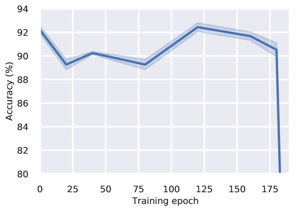
Figure 6: Varying training epochs to test the effects of the convergence of CNNs on the search results of Eq. 9. The total training epoch for pruning ResNet-56 on CIFAR-10 is 200. (The solid line and shadow denote the mean and standard deviation of three experiments, respectively.)

Varying Convergence. The state of convergence in CNNs influence the search results of Eq. 9. To examine the convergence on the search results of Eq. 9, we change the training epoch to test the final search results (In Fig. 6). When the training epoch equals to zero, that is, we prune the model from scratch, the accuracy of the pruned model is about 92.5%. The reason why this setting could achieve good results might be due to the “lottery ticket hypothesis” proposed in [80]. Specifically, randomly initialized networks contain subnetworks (“winning ticket”) that reach test accuracy comparable to the original network. When the training epoch reaches 20 to 80, the accuracy drops to about 89%. This means the preliminary convergence at early epochs is not ideal to search for pruned models and may harm the accuracy. Further increasing the training epoch to 120 would boost the accuracy. The reason is that the convergence at later epochs is sufficient to search for a good pruned model. If the training epoch continues to increase, the accuracy will drop dramatically. This decrease in accuracy is because the network would not have enough training time to recover accuracy from the pruning operation. Since the total training epoch is 200, if the number of training epochs is larger than 180, the remaining epoch is smaller than 20, which is not enough for the network to recover accuracy.

Varying Execution Time. We use four neighboring CNNs in the experimental setting to balance the optimality and execution time. To better understand the influence of the execution time on the pruning results, we change the number of candidate neighboring CNNs so that the execution time could change. The results are shown in Fig. 7. Generally, when we increase the number of neighboring CNNs from 2 to 5, the execution time would increase from 42 seconds to 63 seconds, and the accuracy would increase. This is because a larger search space is beneficial to the final accuracy. We also find that if execution time keeps increasing, the accuracy improvement will gradually become smaller. For example, increasing the execution time from 50 to 55 would lead to about 0.20% accuracy improvement. In contrast, increasing the execution time from 57 to 62 would lead to only 0.03% accuracy improvement. These results also demonstrate that our scope of search is appropriately defined. Further increasing the execution time or the scope of search does not bring considerable improvement.

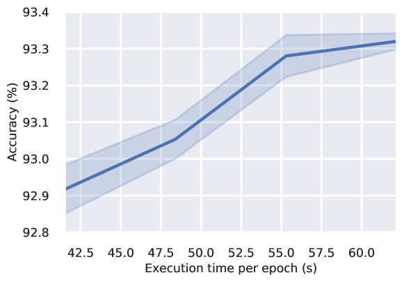
Figure 7: Varying execution time to test accuracies of pruned models. (The solid line and shadow denote the mean and standard deviation of three experiments, respectively.)

IV-G Analysis of Pearson Correlation Based Criterion

We test the criterion that removes the filters that have a large Pearson correlation [81] with other filters. It shows that our meta-process succeeds in excluding bad criteria during training.

Single Criterion. First, we compare the Pearson correlation-based method with the Minkowski distance-based criterion without meta-process, that is, only one criterion is utilized. The results are shown in Table VI. The Pearson correlation-based criterion is about 27% less accurate than the Minkowski distance-based criterion when pruning the scratch models and has about 17% less accuracy when pruning the pre-trained models. It is clear that the Pearson correlation-based criterion is not as effective as the Minkowski distance-based criterion to serve as a pruning criterion in our framework.

Criteria	pretrain?	Accuracy (%)
Minkowski	✗	92.37 ($\pm$0.30)
Pearson	✗	65.01 ($\pm$10.07)
Minkowski	✓	93.37 ($\pm$0.13)
Pearson	✓	75.19 ($\pm$11.87)

TABLE VI: Pruning scratch and pre-trained ResNet-56 on CIFAR-10 with different criteria.

Multiple Criteria. In order to see whether the Pearson correlation-based criterion will be chosen in the meta-process in Eq. 9, we add the Pearson correlation-based criterion as an additional candidate pruning criterion in the meta-process. The other four criteria are the same in the experiment settings in Section IV-B. After examining the meta-process during the whole training process, we find that the Pearson correlation-based criterion is not selected. This result also shows that the Pearson correlation-based criterion is not an essential pruning criterion in our framework.

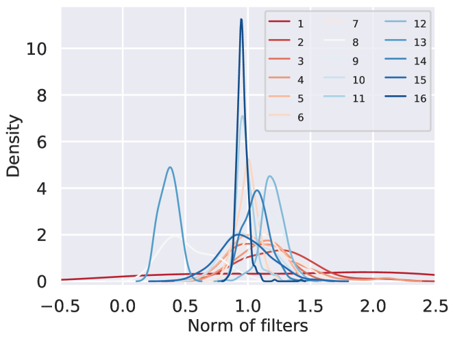
Figure 8: Norm distribution of filters from different layers of ResNet-18 on ILSVRC-2012. Different colors represent different layers. The density is obtained with Kernel Distribution Estimate (KDE) of the norm distribution.

Explanation. To comprehensively understand the network, we plot the kernel distribution estimate (KDE) [82] for the norm distribution of all convolutional layers, as shown in Fig. 8. The norm distribution reflects the weight values of the filters. From the figure, we find that the lower layers have a broader range of norms than the upper layers. For example, the range of the norm of the first layer (indicated by the deep red line) is [0.5, 1.5], and the range of norm of the $16_{th}$ layer is [0.8, 1.1]. Since different layers have different functions [20], these results imply that in neural networks, different functions are achieved by different filter values. The above phenomenon may account for the Pearson correlation-based criterion is not a suitable pruning criterion. A key mathematical property of the Pearson correlation coefficient [81] is that the Pearson correlation coefficient of two variables $X$ and $Y$ is invariant under changes in location and scale in these two variables. Specifically, transforming a variable $X$ to $a+bX$ would not change the Pearson correlation coefficient. Therefore, the Pearson correlation-based criterion could not distinguish different functions in the neural network, where the location and scale are crucial for conducting different functions.

IV-H Analysis of Cosine Distance Based Criterion

We also test the measure based on cosine distance [83] in Table VII. “Only Cosine” means just the cosine distance criterion is used as the pruning criterion, while “Multiple” indicates five criteria, including cosine distance criterion and four criteria listed in section IV. B. We find that cosine distance criterion has low accuracy and is not suitable for pruning. Moreover, in the “Multiple” setting, we find the cosine distance criterion is never selected by our meta-process. This means that our meta-process succeed in excluding the bad criterion, such as the cosine distance criterion, during the process of decision.

Criteria	pretrain?	Accuracy (%)
Only Cosine	✗	72.33 ($\pm$13.22)
Multiple	✗	92.29 ($\pm$0.13)
Only Cosine	✓	71.61 ($\pm$4.98)
Multiple	✓	93.32 ($\pm$0.07)

TABLE VII: Pruning ResNet-56 on CIFAR-10 with cosine distance criterion. “Multiple” means five criteria including cosine distance criterion and four criteria listed in section IV. B.

Weighted Criteria	Selected Index	Accuracy (%)
Norm-1 + Dist-1	[3,13,4,15]	93.69 ($\pm$0.07)
Norm-1 + Pearson	[4,3,0,15]	92.25 ($\pm$0.68)
Dist-1 + Pearson	[4,3,0,13]	92.26 ($\pm$1.26)
Norm-1 + Dist-1 + Pearson	[4,3,13,15]	93.40 ($\pm$0.08)

TABLE VIII: Pruning ResNet-56 on CIFAR-10 with different weighted criteria. “Selected Index” means the index of pruned filters in the first convolutional layer.

IV-I Analysis of Weighted Criteria

We further examine the results of weighted criteria, and the results are shown in Table VIII. Specifically, we first obtain the rankings under each criterion. Then we calculate the average ranking for several candidate criteria. In this way, the average ranking can be viewed as the ranking of weighted criteria. We do not use the importance scores because the importance scores for different criteria has various ranges, which makes the weighting process difficult. In Table VIII, “Norm-1 + Dist-1” means the weighted criteria for $\ell_{1}$-norm-based criterion and Manhattan distance-based criterion. It is clear that “Norm-1 + Dist-1” achieves the best performance because both $\ell_{1}$-norm-based criterion and Manhattan distance-based criterion are good for pruning. In contrast, other weighted criteria containing the Pearson criterion obtain smaller accuracy than “Norm-1 + Dist-1”. These results show that it is difficult for the weighted criteria to exclude the “bad effects” of bad criteria such as the Pearson criterion.

IV-J Feature Map Visualization and Explanation

We visualize the feature maps of the first layer of the first block of ResNet-18, as shown in Fig. 5. We rank the 64 channel in this layer with number 0 to 63 and set the pruning rate to 10% to choose six filters to be pruned. We select the channel (44, 29, 62, 56, 30, 51) via the $L2$-norm criterion and select the channel (44, 56, 29, 51, 52, 24) via Euclidean distance criterion. For both criteria, we select channel (29, 44, 51, 56), but order of the channels is different.

We focus on the different channels selected by these criteria to illustrate their difference. In addition to the common part, the norm-based criterion select (30, 62), while the distance-based criterion select (24, 52). Channel (30, 62) have rather small activation values and might be meaningless to the network, so they are selected by the norm-based criterion. For channel (24, 52), the rough shapes of the cat in these channels are similar to other channels such as (17, 23, 25, 32, 59), so the distance-based criterion (relational criterion) prefers to prune these channels. These results validate our points that norm-based criterion and distance-based criterion consider different aspects of the network. In this way, during the updating of the network and the filter distribution, adaptively selecting those criteria is necessary.

V Conclusion and Future Work

In this paper, we propose a new Meta-attribute-based Filter Pruning (MFP) strategy for deep CNNs acceleration. Unlike the existing norm-based criterion, MFP explicitly considers the geometric information between filters. Furthermore, as a meta-framework, MFP adaptively selects the suitable criteria during training to fit the current filter distribution. Results show that MFP advances the state-of-the-art methods in several benchmarks. In the future, we could consider utilizing different criteria for different layers of the network. Even within a network layer, we could combine different criteria for filter pruning. Besides, whether a better meta-attribute exists is yet to be explored. Moreover, other parallel acceleration algorithms, such as low-precision weights, could be used as a complementary method to improve the performance further.

VI ACKNOWLEDGEMENT

This work was supported by the Australian Research Council (ARC) under Grant DP200100938.

Yang He received the B.S. degree and MSc from the University of Science and Technology of China, Hefei, China, in 2014 and 2017, respectively. He is expected to obtain Ph.D. degree at the University of Technology Sydney in 2022. He is currently a scientist at A*STAR Centre for Frontier AI Research (CFAR), Singapore. His research interests include deep learning, computer vision, and filter pruning.

Ping Liu is currently a scientist at A*STAR Centre for Frontier AI Research (CFAR), Singapore. Before joining CFAR, he was a research staff with the Center for Artificial Intelligence, University of Technology Sydney, Sydney, AUS. He received his Ph.D. degree in the Department of Computer Science and Engineering, University of South Carolina, SC, USA. He got his Master Degree from Huazhong University of Science and Technology, WuHan, China; Bachelor Degree from Wuhan University of Technology, WuHan, China. His research interests include computer vision, machine learning, and deep learning.

Linchao Zhu is currently a Lecturer and core member of the Australian Artificial Intelligence Institute (AAII), University of Technology Sydney. He received his Ph.D. degree in University of Technology Sydney. He graduated from Zhejiang University with a bachelor’s degree. His research interests include video representation learning, unsupervised learning, self-supervised learning, few-shot learning, transfer learning, model efficiency.

Yi Yang received the Ph.D. degree in computer science from Zhejiang University, Hangzhou, China, in 2010. He is currently a distinguished professor with Zhejiang University, China. Professor Yi Yang is an unremunerated Adjunct Professor with the Australian Artificial Intelligence Institute (AAII), University of Technology Sydney, Australia. He was a professor and Director of the ReLER Lab at the Australian Artificial Intelligence Institute (AAII), University of Technology Sydney, Australia. He was a Post-Doctoral Research with the School of Computer Science, Carnegie Mellon University, Pittsburgh, PA, USA. His current research interest include machine learning and its applications to multimedia content analysis and computer vision, such as multimedia indexing and retrieval, surveillance video analysis and video semantics understanding.

References

- [1] B. Frénay and M. Verleysen, “Classification in the presence of label noise: a survey,” IEEE transactions on neural networks and learning systems, vol. 25, no. 5, pp. 845–869, 2013.
- [2] Y. Yan, F. Nie, W. Li, C. Gao, Y. Yang, and D. Xu, “Image classification by cross-media active learning with privileged information,” IEEE Transactions on Multimedia, vol. 18, no. 12, pp. 2494–2502, 2016.
- [3] M. Gong, J. Zhao, J. Liu, Q. Miao, and L. Jiao, “Change detection in synthetic aperture radar images based on deep neural networks,” IEEE transactions on neural networks and learning systems, vol. 27, no. 1, pp. 125–138, 2015.
- [4] X. Zhang, Y. Wei, Y. Yang, and T. Huang, “Self-produced guidance for weakly-supervised object localization,” IEEE Transactions on Cybernetics, 2020.
- [5] Y. Yang, Z. Ma, A. G. Hauptmann, and N. Sebe, “Feature selection for multimedia analysis by sharing information among multiple tasks,” IEEE Transactions on Multimedia, vol. 15, no. 3, pp. 661–669, 2012.
- [6] L. Zhu, H. Fan, Y. Luo, M. Xu, and Y. Yang, “Temporal cross-layer correlation mining for action recognition,” IEEE Transactions on Multimedia, 2021.
- [7] K. Simonyan and A. Zisserman, “Very deep convolutional networks for large-scale image recognition,” in ICLR, 2015.
- [8] K. He, X. Zhang, S. Ren, and J. Sun, “Deep residual learning for image recognition,” in CVPR, 2016.
- [9] S. Han, J. Pool, J. Tran, and W. Dally, “Learning both weights and connections for efficient neural network,” in NIPS, 2015.
- [10] M. A. Carreira-Perpinán and Y. Idelbayev, “Learning-compression” algorithms for neural net pruning,” in CVPR, 2018.
- [11] H. Li, A. Kadav, I. Durdanovic, H. Samet, and H. P. Graf, “Pruning filters for efficient ConvNets,” in ICLR, 2017.
- [12] R. Yu, A. Li, C.-F. Chen, J.-H. Lai, V. I. Morariu, X. Han, M. Gao, C.-Y. Lin, and L. S. Davis, “Nisp: Pruning networks using neuron importance score propagation,” in CVPR, 2018.
- [13] Y. Guo, A. Yao, and Y. Chen, “Dynamic network surgery for efficient DNNs,” in NIPS, 2016.
- [14] Y. He, G. Kang, X. Dong, Y. Fu, and Y. Yang, “Soft filter pruning for accelerating deep convolutional neural networks,” in IJCAI, 2018.
- [15] W. Chen, Y. Zhang, D. Xie, and S. Pu, “A layer decomposition-recomposition framework for neuron pruning towards accurate lightweight networks,” in AAAI, vol. 33, 2019, pp. 3355–3362.
- [16] S. Lin, R. Ji, X. Guo, X. Li et al., “Towards convolutional neural networks compression via global error reconstruction.” in IJCAI, 2018.
- [17] D. Wang, L. Zhou, X. Bai, and J. Zhou, “A one-step pruning-recovery framework for acceleration of convolutional neural networks,” arXiv preprint arXiv:1906.07488, 2019.
- [18] X. Dai, H. Yin, and N. K. Jha, “Grow and prune compact, fast, and accurate lstms,” arXiv preprint arXiv:1805.11797, 2018.
- [19] J. Ye, X. Lu, Z. Lin, and J. Z. Wang, “Rethinking the smaller-norm-less-informative assumption in channel pruning of convolution layers,” in ICLR, 2018.
- [20] J. Yosinski, J. Clune, A. Nguyen, T. Fuchs, and H. Lipson, “Understanding neural networks through deep visualization,” in ICML Workshop on Deep Learning, 2015.
- [21] A. Singh, A. Yadav, and A. Rana, “K-means with three different distance metrics,” International Journal of Computer Applications, vol. 67, no. 10, 2013.
- [22] P. B. Brazdil, C. Soares, and J. P. Da Costa, “Ranking learning algorithms: Using ibl and meta-learning on accuracy and time results,” Machine Learning, vol. 50, no. 3, pp. 251–277, 2003.
- [23] S. Han, H. Mao, and W. J. Dally, “Deep compression: Compressing deep neural networks with pruning, trained quantization and huffman coding,” in ICLR, 2015.
- [24] F. Tung and G. Mori, “Clip-q: Deep network compression learning by in-parallel pruning-quantization,” in CVPR, 2018.
- [25] T. Zhang, S. Ye, K. Zhang, J. Tang, W. Wen, M. Fardad, and Y. Wang, “A systematic dnn weight pruning framework using alternating direction method of multipliers,” ECCV, 2018.
- [26] X. Dong, S. Chen, and S. Pan, “Learning to prune deep neural networks via layer-wise optimal brain surgeon,” in Advances in Neural Information Processing Systems, 2017, pp. 4857–4867.
- [27] W. Wen, C. Wu, Y. Wang, Y. Chen, and H. Li, “Learning structured sparsity in deep neural networks,” in NIPS, 2016.
- [28] V. Lebedev and V. Lempitsky, “Fast ConvNets using group-wise brain damage,” in CVPR, 2016.
- [29] H. Hu, R. Peng, Y.-W. Tai, and C.-K. Tang, “Network trimming: A data-driven neuron pruning approach towards efficient deep architectures,” arXiv preprint arXiv:1607.03250, 2016.
- [30] Z. Liu, J. Li, Z. Shen, G. Huang, S. Yan, and C. Zhang, “Learning efficient convolutional networks through network slimming,” in ICCV, 2017.
- [31] J.-H. Luo, J. Wu, and W. Lin, “ThiNet: A filter level pruning method for deep neural network compression,” in ICCV, 2017.
- [32] Y. He, X. Zhang, and J. Sun, “Channel pruning for accelerating very deep neural networks,” in ICCV, 2017.
- [33] P. Molchanov, S. Tyree, T. Karras, T. Aila, and J. Kautz, “Pruning convolutional neural networks for resource efficient transfer learning,” in ICLR, 2017.
- [34] A. Dubey, M. Chatterjee, and N. Ahuja, “Coreset-based neural network compression,” arXiv preprint arXiv:1807.09810, 2018.
- [35] X. Suau, L. Zappella, V. Palakkode, and N. Apostoloff, “Principal filter analysis for guided network compression,” arXiv preprint arXiv:1807.10585, 2018.
- [36] D. Wang, L. Zhou, X. Zhang, X. Bai, and J. Zhou, “Exploring linear relationship in feature map subspace for convnets compression,” arXiv preprint arXiv:1803.05729, 2018.
- [37] Z. Zhuang, M. Tan, B. Zhuang, J. Liu, Y. Guo, Q. Wu, J. Huang, and J. Zhu, “Discrimination-aware channel pruning for deep neural networks,” in NIPS, 2018.
- [38] Q. Huang, K. Zhou, S. You, and U. Neumann, “Learning to prune filters in convolutional neural networks,” in 2018 IEEE Winter Conference on Applications of Computer Vision (WACV). IEEE, 2018, pp. 709–718.
- [39] Y. He and S. Han, “Adc: Automated deep compression and acceleration with reinforcement learning,” arXiv preprint arXiv:1802.03494, 2018.
- [40] S. Lin, R. Ji, Y. Li, C. Deng, and X. Li, “Toward compact convnets via structure-sparsity regularized filter pruning,” IEEE transactions on neural networks and learning systems, vol. 31, no. 2, pp. 574–588, 2019.
- [41] Z. Chen, T.-B. Xu, C. Du, C.-L. Liu, and H. He, “Dynamical channel pruning by conditional accuracy change for deep neural networks,” IEEE Transactions on Neural Networks and Learning Systems, 2020.
- [42] J. Wang, C. Xu, X. Yang, and J. M. Zurada, “A novel pruning algorithm for smoothing feedforward neural networks based on group lasso method,” IEEE transactions on neural networks and learning systems, vol. 29, no. 5, pp. 2012–2024, 2017.
- [43] M. Lin, L. Cao, S. Li, Q. Ye, Y. Tian, J. Liu, Q. Tian, and R. Ji, “Filter sketch for network pruning,” IEEE Transactions on Neural Networks and Learning Systems, 2021.
- [44] M. Lin, R. Ji, S. Li, Y. Wang, Y. Wu, F. Huang, and Q. Ye, “Network pruning using adaptive exemplar filters,” IEEE Transactions on Neural Networks and Learning Systems, 2021.
- [45] S. Lin, R. Ji, C. Chen, D. Tao, and J. Luo, “Holistic cnn compression via low-rank decomposition with knowledge transfer,” IEEE transactions on pattern analysis and machine intelligence, vol. 41, no. 12, pp. 2889–2905, 2018.
- [46] M. Kang and B. Han, “Operation-aware soft channel pruning using differentiable masks,” in International Conference on Machine Learning, 2020.
- [47] S. Gao, F. Huang, W. Cai, and H. Huang, “Network pruning via performance maximization,” in CVPR, 2021.
- [48] X. Ning, T. Zhao, W. Li, P. Lei, Y. Wang, and H. Yang, “Dsa: More efficient budgeted pruning via differentiable sparsity allocation,” in ECCV, 2020.
- [49] H. Zhuo, X. Qian, Y. Fu, H. Yang, and X. Xue, “Scsp: Spectral clustering filter pruning with soft self-adaption manners,” arXiv preprint arXiv:1806.05320, 2018.
- [50] Y. He, P. Liu, Z. Wang, Z. Hu, and Y. Yang, “Filter pruning via geometric median for deep convolutional neural networks acceleration,” in Proceedings of the IEEE Conference on Computer Vision and Pattern Recognition, 2019, pp. 4340–4349.
- [51] Y. He, X. Dong, G. Kang, Y. Fu, C. Yan, and Y. Yang, “Asymptotic soft filter pruning for deep convolutional neural networks,” IEEE transactions on cybernetics, 2019.
- [52] Y. He, Y. Ding, P. Liu, L. Zhu, H. Zhang, and Y. Yang, “Learning filter pruning criteria for deep convolutional neural networks acceleration,” in Proceedings of the IEEE Conference on Computer Vision and Pattern Recognition (CVPR), 2020.
- [53] Y. He, P. Liu, L. Zhu, and Y. Yang, “Meta filter pruning to accelerate deep convolutional neural networks,” arXiv preprint arXiv:1904.03961, 2019.
- [54] X. Wang, Z. Zheng, Y. He, F. Yan, Z. Zeng, and Y. Yang, “Progressive local filter pruning for image retrieval acceleration,” arXiv preprint arXiv:2001.08878, 2020.
- [55] X. Wang, Z. Zheng, Y. He, F. Yan, Z. Zeng, and Y. Yi, “Soft person re-identification network pruning via block-wise adjacent filter decaying,” IEEE Transactions on Cybernetics, 2022.
- [56] Y. He, P. Liu, Z. Wang, and Y. Yang, “Pruning filter via geometric median for deep convolutional neural networks acceleration,” in CVPR, 2019.
- [57] D. H. Le and B.-S. Hua, “Network pruning that matters: A case study on retraining variants,” in ICLR, 2021.
- [58] S. Sen, N. Moha, B. Baudry, and J.-M. Jézéquel, “Meta-model pruning,” in International Conference on Model Driven Engineering Languages and Systems. Springer, 2009, pp. 32–46.
- [59] T.-W. Chin, C. Zhang, and D. Marculescu, “Layer-compensated pruning for resource-constrained convolutional neural networks,” arXiv preprint arXiv:1810.00518, 2018.
- [60] Z. Liu, H. Mu, X. Zhang, Z. Guo, X. Yang, T. K.-T. Cheng, and J. Sun, “Metapruning: Meta learning for automatic neural network channel pruning,” arXiv preprint arXiv:1903.10258, 2019.
- [61] W. Wang, C. Fu, J. Guo, D. Cai, and X. He, “Cop: Customized deep model compression via regularized correlation-based filter-level pruning,” in IJCAI, 2019.
- [62] P. Molchanov, A. Mallya, S. Tyree, I. Frosio, and J. Kautz, “Importance estimation for neural network pruning,” in CVPR, 2019.
- [63] H. Liu, K. Simonyan, and Y. Yang, “Darts: Differentiable architecture search,” in Proc. Int. Conf. Learn. Represent., 2019.
- [64] M. Tan and Q. Le, “Efficientnet: Rethinking model scaling for convolutional neural networks,” in International Conference on Machine Learning. PMLR, 2019, pp. 6105–6114.
- [65] B. Zoph, V. Vasudevan, J. Shlens, and Q. V. Le, “Learning transferable architectures for scalable image recognition,” in CVPR, 2018.
- [66] D. Sinwar and R. Kaushik, “Study of euclidean and manhattan distance metrics using simple k-means clustering,” Int. J. Res. Appl. Sci. Eng. Technol, vol. 2, no. 5, pp. 270–274, 2014.
- [67] J. C. Gower, “Properties of euclidean and non-euclidean distance matrices,” Linear Algebra and its Applications, vol. 67, pp. 81–97, 1985.
- [68] X. Dong, J. Huang, Y. Yang, and S. Yan, “More is less: A more complicated network with less inference complexity,” in CVPR, 2017.
- [69] Y. He, J. Lin, Z. Liu, H. Wang, L.-J. Li, and S. Han, “Amc: Automl for model compression and acceleration on mobile devices,” in Proceedings of the European Conference on Computer Vision (ECCV), 2018, pp. 784–800.
- [70] Z. Liu, M. Sun, T. Zhou, G. Huang, and T. Darrell, “Rethinking the value of network pruning,” arXiv preprint arXiv:1810.05270, 2018.
- [71] A. Kalhor, B. N. Araabi, and C. Lucas, “Evolving takagi–sugeno fuzzy model based on switching to neighboring models,” Applied Soft Computing, vol. 13, no. 2, pp. 939–946, 2013.
- [72] A. T. Benjamin and J. J. Quinn, Proofs that really count: the art of combinatorial proof. MAA, 2003, no. 27.
- [73] P. Singh, V. K. Verma, P. Rai, and V. P. Namboodiri, “Leveraging filter correlations for deep model compression,” arXiv preprint arXiv:1811.10559, 2018.
- [74] A. Krizhevsky and G. Hinton, “Learning multiple layers of features from tiny images,” 2009.
- [75] O. Russakovsky, J. Deng, H. Su, J. Krause, S. Satheesh, S. Ma, Z. Huang, A. Karpathy, A. Khosla, M. Bernstein et al., “ImageNet large scale visual recognition challenge,” IJCV, 2015.
- [76] S. Zagoruyko, “92.45% on cifar-10 in torch.” http://torch.ch/blog/2015/07/30/cifar.html, 2015.
- [77] S. Zagoruyko and N. Komodakis, “Wide residual networks,” in BMVC, 2016.
- [78] K. He, X. Zhang, S. Ren, and J. Sun, “Identity mappings in deep residual networks,” in ECCV, 2016.
- [79] A. Paszke, S. Gross, S. Chintala, G. Chanan, E. Yang, Z. DeVito, Z. Lin, A. Desmaison, L. Antiga, and A. Lerer, “Automatic differentiation in pytorch,” in NIPS-W, 2017.
- [80] J. Frankle and M. Carbin, “The lottery ticket hypothesis: Finding sparse, trainable neural networks,” in ICLR, 2019.
- [81] J. Benesty, J. Chen, Y. Huang, and I. Cohen, “Pearson correlation coefficient,” in Noise reduction in speech processing. Springer, 2009, pp. 1–4.
- [82] B. W. Silverman, Density estimation for statistics and data analysis. Routledge, 2018.
- [83] J. Ye, “Cosine similarity measures for intuitionistic fuzzy sets and their applications,” Mathematical and computer modelling, vol. 53, no. 1-2, pp. 91–97, 2011.