Higher Dimensional Particle Model in Third-Order Lovelock Gravity

Abstract

By using the formalism of thin-shells, we construct a geometrical model of a particle in third-order Lovelock gravity. This particular theory which is valid at least in $7$ dimensions, provides enough degrees of freedom and grounds towards such a construction. The particle consists of a flat interior and a non-black hole exterior spacetimes whose mass, charge and radius are determined from the junction conditions, in terms of the parameters of the theory.

I Introduction

Geometrical description of elementary particles attracted interest of physicists at different stages of physics history Vilenkin1 ; Vilenkin2 . With the advent of general relativity all attempts in that direction focused on the curvatures and singularities of spacetimes as potential sites to represent particles. In his description, Geometrodynamics Wheeler1 , John Wheeler advocated the view of concentrated field points - the Geons - as particle-like structures in spacetimes. More recently, the trend of constructing particle models from geometry oriented towards non-singular spacetimes such as the de Sitter core with the cosmological constant. Since a particle can also have charge besides mass, the electromagnetic spacetimes such as the non-singular Bertotti-Robinson geometry Bertotti1 ; Robinson1 also attracted attentions Zaslavskii1 in this regard. Having no interior singularity and possessing both mass and electric charge became basic criteria in search for a geometrical model of particles. The method has been to consider a spherical shell as the representative surface of the particle with inner/outer regions satisfying certain junction conditions. Among those conditions we cite the continuity of the first fundamental form (the metric) and a possible surface energy-momentum tensor emerging from the discontinuity conditions of the second fundamental form (the extrinsic curvature).

In this article, we show that geometrical model of a particle is possible within the context of third-order Lovelock gravity (TOLG) combined with the thin-shell formalism. Lovelock gravity (LG) Lovelock1 , is known to have the most general combination of curvature invariants that still maintains the second-order field equations. Our model will cover up to the third-order terms, supplemented by the Maxwell Lagrangian, apt for $n+1$-dimensional spacetimes with $n\geq 6$, in which the theory admits non-trivial solutions. The motivation to choose TOLG is based on the fact that the number of parametric degrees of freedom in this gravity theory, due to its free parameters (coupling constants in the Lagrangian densities of the action), allows us to overcome the restrictions imposed by the junction conditions to eventually find sensible expressions for the mass, the radius and other parameters of the particle. We made choice amongst available solutions of the theory that suits our purpose. A spherical thin-shell is assumed as the surface of the particle, whose inside is the flat Minkowski spacetime, accompanied with a suitable Lovelock solution to represent the outer region. Let us add that in Einstein’s gravity a constant potential inside the shell ($\Phi=$constant$\neq 0$) amounts to the presence of a global monopole at the origin. To avoid any physical inconvenience invited by such a monopole, we can choose the interior geometry of our particle to be represented by the flat Minkowski metric, i.e., $\Phi=0$, which is the simplest case to be chosen and is also in accord with Birkhoff’s theorem Birkhoff1 . Deliberate choice of the Lovelock’s coupling constants in the action, renders physical boundary conditions possible for a surface energy-momentum on the shell. As the final step, we set the pressure and surface energy density to zero and search for viable geometrical criteria. Those conditions determine the mass and charge of the particle constructed, entirely from the geometrical parameters of the third-order Lovelock gravity in $6+1$ dimensions, as an example.

Overall, the article is organized in the following sections. In section II, rather than the thin-shell formalism in general, the particular choices of inner/outer solutions within the third-order Lovelock gravity framework are introduced. In section III, we briefly review the proper junction conditions for a thin-shell in the third-order Lovelock gravity. Section IV is devoted to conclusion. All over the article, the unit convention $4\pi\varepsilon_{0\left(n+1\right)}=8\pi G_{\left(n+1\right)}=\hslash=c=1$ is applied.

II Thin-Shell Formalism

Consider a spherically symmetric Riemannian manifold in $n+1$ dimensions, with two distinct regions, say $\left(\Sigma,g\right)^{\pm}=\{x_{\pm}^{\mu}|r_{+}\geq a>r_{e},r_{-}\leq a\}$ (where $r_{e}$ is a (probable) event horizon), distinguished by their common timelike hypersurface $\partial\Sigma=\{\xi_{\pm}^{\mu}|r=a\}$. The hypersurface $\partial\Sigma$ is therefore a thin-shell separating the two regions with different line elements and probably different coordinates $x_{\pm}^{\mu}$. The inner spacetime (marked with $\left(-\right)$) is (preferably) non-singular and the outer spacetime (marked with $\left(+\right)$) has its event horizon behind the thin–shell (if there is any). For the purpose of this study, we would like to have for both inner and outer spacetimes, the solutions to the TOLG. Expectedly, the two spacetimes cannot be matched randomly at the thin-shell location, and it takes some proper junction conditions which are discussed below.

In the $n+1$-dimensional TOLG ($n\geq 6$), the action is given by

$$I=\int d^{n+1}x\sqrt{-g}\left(\alpha_{1}\mathcal{L}_{1}+\alpha_{2}\mathcal{L}_{2}+\alpha_{3}\mathcal{L}_{3}-F^{\mu\nu}F_{\mu\nu}\right),$$ (1)

where the electromagnetic field is presented by the anti-symmetric field tensor $F_{\mu\nu}$. Here,

$$\mathcal{L}_{1}=\mathcal{L}_{\text{EH}}=R,$$ (2)

$$\mathcal{L}_{2}=\mathcal{L}_{\text{GB}}=R^{\kappa\lambda\mu\nu}R_{\kappa\lambda\mu\nu}-4R^{\mu\nu}R_{\mu\nu}+R^{2},$$ (3)

and

$$\mathcal{L}_{3}=\mathcal{L}_{\text{TOLG}}=2R^{\kappa\lambda\rho\sigma}R_{\rho\sigma\mu\nu}R_{\hskip 8.5359pt\kappa\lambda}^{\mu\nu}+8R_{\hskip 8.5359pt\kappa\lambda}^{\mu\nu}R_{\hskip 8.5359pt\nu\rho}^{\kappa\sigma}R_{\hskip 8.5359pt\mu\sigma}^{\lambda\rho}+24R^{\kappa\lambda\mu\nu}R_{\mu\nu\lambda\rho}R_{\hskip 4.26773pt\kappa}^{\rho}\\ +3RR^{\kappa\lambda\mu\nu}R_{\kappa\lambda\mu\nu}+24R^{\kappa\lambda\mu\nu}R_{\mu\kappa}R_{\nu\lambda}+16R^{\mu\nu}R_{\nu\sigma}R_{\hskip 4.26773pt\mu}^{\sigma}-12RR^{\mu\nu}R_{\mu\nu}+R^{3}$$ (4)

are the first (Einstein-Hilbert (EH)), the second (Gauss-Bonnet (GB)), and the third Lagrangian densities of LG, respectively, accompanied with their respective constant coefficients $\alpha_{1}\equiv 1$, $\alpha_{2}$, and $\alpha_{3}$. The spherically symmetric line element suitable for this action is given by

$$ds^{2}=-f\left(r\right)dt^{2}+f^{-1}\left(r\right)dr^{2}+r^{2}d\Omega_{n-1}^{2},$$ (5)

where $d\Omega_{n-1}^{2}$ is the line element of the $n-1$-dimensional unit sphere. Although there are three general solutions for $f\left(r\right)$, the one we consider here is (see Amirabi1 ; Mehdizadeh1 and references therein)

$$f\left(r\right)=1-r^{2}\left(-\frac{\tilde{\alpha}_{2}}{3\tilde{\alpha}_{3}}+\delta+u\delta^{-1}\right),$$ (6)

where

$$\left\{\begin{array}[]{c}\tilde{\alpha}_{2}=\left(n-3\right)\left(n-2\right)\alpha_{2}\\ \tilde{\alpha}_{3}=\left(n-5\right)\left(n-4\right)\left(n-3\right)\left(n-2\right)\alpha_{3}\\ \delta=\left(v+\sqrt{v^{2}-u^{3}}\right)^{1/3}\end{array}\right.,$$ (7)

and

$$\left\{\begin{array}[]{c}u=\dfrac{\tilde{\alpha}_{2}^{2}-3\tilde{\alpha}_{3}}{9\tilde{\alpha}_{3}^{2}}\\ v=\dfrac{9\tilde{\alpha}_{2}\tilde{\alpha}_{3}-2\tilde{\alpha}_{2}^{3}}{54\tilde{\alpha}_{3}^{3}}+\dfrac{1}{2\tilde{\alpha}_{3}}\left[\dfrac{m}{r^{n}}-\dfrac{q^{2}}{r^{2\left(n-1\right)}}\right]\end{array}\right..$$ (8)

In the special case where $\tilde{\alpha}_{2}^{2}=3\tilde{\alpha}_{3}=\beta^{2}$, one finds $u=0$ and $\delta=\left(2v\right)^{1/3}$, with which the solution in Eq. (6) reduces to

$$f\left(r\right)=1+\frac{r^{2}}{\beta}\left\{1-\left[1+3\beta\left(\frac{m}{r^{n}}-\frac{q^{2}}{r^{2\left(n-1\right)}}\right)\right]^{\frac{1}{3}}\right\}.$$ (9)

Depending on the values of the mass $m$, the charge $q$, and the number of spatial dimensions $n$, this particular solution could represent a black hole with two horizons, an extremal black hole with a single horizon, or a non-black hole solution with a naked singularity. It is worth-mentioning that although $m$ and $q$ are linearly proportional to the real mass and charge of the spacetime, they are dimension-dependent parameters. In this study, we assign to the inner spacetime an $n+1$-dimensional Minkowski geometry, which amounts to choosing $m_{-}=q_{-}=0$ in (8), hence, from Eq. (6) $f_{-}\left(r_{-}\right)=1$. Furthermore, we consider $m_{+}=m$, $q_{+}=q$, and $\tilde{\alpha}_{2+}^{2}=3\tilde{\alpha}_{3+}=\beta_{+}^{2}$ for the outer spacetime, while $a>r_{e}$, where $r_{e}$ is the event horizon of $f_{+}\left(r_{+}\right)$ (if there is any); so $f_{+}\left(r_{+}\right)$ has the general form in Eq. (9). This choice for the outer spacetime only simplifies the calculations so that we state our claim stronger. Of course, the same analysis could be conducted without imposing $\tilde{\alpha}_{2+}^{2}=3\tilde{\alpha}_{3+}=\beta_{+}^{2}$. Moreover, although with the choice $f_{-}\left(r_{-}\right)=1$ we exploited a Minkowski spacetime for the inner region of the particle, the coupling constants $\tilde{\alpha}_{2-}$ and $\tilde{\alpha}_{3-}$ remain arbitrary, which will play role in determining the mass and the charge of the particle. Let us emphasize that for $m=q=0$ inside the shell by virtue of Eqs. (6-8) and arbitrary $\tilde{\alpha}_{2-}$ and $\tilde{\alpha}_{3-}$ we obtain $f_{-}\left(r_{-}\right)=1$, to conform with the Birkhoff’s theorem. In the next section, this will arise (see Eq. (19) below) explicitly.

III The Junction Conditions

As it is already mentioned, the matching at $r_{\pm}=a$ follows certain junction conditions. In general relativity these are known as Darmois-Israel junction conditions Darmois1 ; Israel1 which are, however, inapplicable when it comes to modified theories of gravity. In the case of TOLG, the proper junction conditions are given by Dehghani et.al in Dehghani1 ; Dehghani2 (Also see Mehdizadeh1 ; Dehghani3 ). These junction conditions firstly demand the continuity of the first fundamental form at the thin-shell’s surface, so one has a smooth transition across the shell. The line element of the thin-shell that can be stated as

$$ds_{\partial\Sigma}^{2}=\gamma_{ab}d\xi^{a}d\xi^{b}=-d\tau^{2}+a^{2}d\Omega_{n-1}^{2},$$ (10)

is therefore unique, where $\tau$ is the proper time on the shell and $\gamma_{ab}^{\pm}=\frac{\partial x_{\pm}^{\mu}}{\partial\xi^{a}}\frac{\partial x_{\pm}^{\nu}}{\partial\xi^{b}}g_{\mu\nu}^{\pm}$ are the induced metric components. Secondly, there exists a non-zero surface energy-momentum tensor on the shell $S_{b}^{a}$, with their components given by Dehghani3

$$S_{b}^{a}=\mathcal{T}_{b+}^{a}-\mathcal{T}_{b-}^{a},$$ (11)

in which

$$\mathcal{T}_{b}^{a}=-\sum_{p=0}^{n}\sum_{s=0}^{p-1}\frac{4^{p-s}p!\alpha_{p}}{2^{p+1}s!\left(2p-2s-1\right)!!}\mathcal{H}_{b}^{\left(p,s\right)a},$$ (12)

where

$$\mathcal{H}_{b}^{\left(p,s\right)a}=\delta_{\left[b_{\,1}\ldots b_{\,2p-1}b\right]}^{\left[a_{1}\ldots a_{2p-1}a\right]}\times R_{\quad\>\>a_{1}a_{2}}^{b_{1}b_{2}}\cdots R_{\quad\quad\quad a_{2s-1}a_{2s}}^{b_{2s-1}b_{2s}}K_{a_{2s+1}}^{b_{2s+1}}K_{a_{2p-1}}^{b_{2p-1}}.$$ (13)

The expression for $\mathcal{T}_{b}^{a}$ is explicitly given in Eq. (B4) of Mehdizadeh1 . To calculate the mixed tensor components $K_{b}^{a}$ of the extrinsic curvature tensor of the shell, we shall use the explicit form

$$K_{ab}^{\pm}=-n_{\lambda}^{\pm}\left(\frac{\partial^{2}x_{\pm}^{\lambda}}{\partial\xi^{a}\partial\xi^{b}}+\Gamma_{\alpha\beta}^{\lambda\pm}\frac{\partial x_{\pm}^{\alpha}}{\partial\xi^{a}}\frac{\partial x_{\pm}^{\beta}}{\partial\xi^{b}}\right),$$ (14)

where $n_{\lambda}^{\pm}$ are the unit spacelike normals to the surface identified by the conditions $n_{\mu}^{\pm}\frac{\partial x_{\pm}^{\mu}}{\partial\xi^{i}}=0$ and $n_{\mu}^{\pm}n_{\pm}^{\mu}=1$, while $\Gamma_{\alpha\beta}^{\lambda\pm}$ are the Christoffel symbols of the outer and inner spacetimes, compatible with $g_{\alpha\beta}^{\pm}$. Note that, since the metric of our bulks are diagonal, for our radially symmetric static timelike shell, the extrinsic curvature tensor will be diagonal, as well. Therefore, tensors $J_{ab}$ and $P_{ab}$ in Eq. (B4) of Mehdizadeh1 , are also diagonal. In this case, their corresponding mixed tensor components could mathematically be cast into the form

$$\left\{\begin{array}[]{c}J_{b}^{a}=diag\left(-\frac{2!}{3}\left\{\sum_{s=0}^{2}\frac{\left(-1\right)^{s}}{n}\binom{n}{s}\left[sK_{\tau}^{\tau}+\left(n-s\right)K_{\theta}^{\theta}\right]\left(K_{\theta}^{\theta}\right)^{s-1}\left(K_{b}^{a}\right)^{5-s}\right\}\right)\\ P_{b}^{a}=diag\left(\frac{4!}{5}\left\{\sum_{s=0}^{4}\frac{\left(-1\right)^{s}}{n}\binom{n}{s}\left[sK_{\tau}^{\tau}+\left(n-s\right)K_{\theta}^{\theta}\right]\left(K_{\theta}^{\theta}\right)^{s-1}\left(K_{b}^{a}\right)^{5-s}\right\}\right)\end{array}\right..$$ (15)

Here, $K_{\tau}^{\tau}$ and $K_{\theta}^{\theta}$ are the components associated with the time and angular coordinates of the thin-shell, since $K_{\theta}^{\theta}=K_{\theta_{1}}^{\theta_{1}}=K_{\theta_{2}}^{\theta_{2}}=...=K_{\theta_{n-1}}^{\theta_{n-1}}.$ Also, $\left(K_{b}^{a}\right)^{p}=K_{c_{1}}^{a}K_{c_{2}}^{c_{1}}\ldots K_{b}^{c_{p-1}}$. In what follows we take $n=6$, noting that the same argument can be applied to higher dimensions, at equal ease.

Having everything done on the second junction conditions, we arrive at

$$\left\{\begin{array}[]{c}\sigma=-\frac{1}{3a^{5}}\sum_{i=+,-}i\sqrt{f_{i}}\left\{15a^{4}+10\tilde{\alpha}_{2i}a^{2}\left(3-f_{i}\right)+3\tilde{\alpha}_{3i}\left(15-10f_{i}+3f_{i}^{2}\right)\right\}\\ p=\frac{1}{2a^{4}}\sum_{i=+,-}\frac{1}{i\sqrt{f_{i}}}\left\{f_{i}^{\prime}a^{4}+8f_{i}a^{3}+\tilde{\alpha}_{2i}a\left[2af_{i}^{\prime}\left(1-f_{i}\right)+8f_{i}\left(1-f_{i}/3\right)\right]+3\tilde{\alpha}_{3i}f_{i}^{\prime}\left(1-f_{i}\right)^{2}\right\}\end{array}\right.,$$ (16)

which are the surface energy density and angular pressure of the emergent fluid on the shell, in accordance with the energy-momentum tensor $S_{b}^{a}=diag\left(-\sigma,p,p,...,p\right)$, respectively. (The extra condition $\tilde{\alpha}_{2+}^{2}=3\tilde{\alpha}_{3+}=\beta_{+}^{2}$ shall be considered.) Next step would be to set equal to zero the energy density and the pressure Vilenkin2 ; Zaslavskii1 and to solve for the mass and the charge of the particle in terms of the radius $a$ and the coupling constants $\tilde{\alpha}_{2-}$, $\tilde{\alpha}_{3-}$ and $\beta_{+}$. However, since we have the freedom to add one more condition, we consider a reasonable assumption to obtain the radius of the particle as well. Nonetheless, note that this assumption is not necessary but it is useful since it enormously decreases the volume of the calculations. To do this, let us go back to the first junction condition for a moment. A unique line element for the shell when it is approached from the two sides (inside and outside) leads to $\dot{t}_{\pm}=f_{\pm}^{-1/2}$, in which an overdot stands for a total derivative with respect to the proper time $\tau$ of the shell. For our assumption, let us take $\dot{t}_{-}=\dot{t}_{+}$, which results in $f_{-}=f_{+}$ at the shell. Therefore, by setting $f_{+}$ from Eq. (9) at $r=a$ to unity for $f_{-}$ and solving for the radius $a$, we obtain

$$a=\left(q^{2}/m\right)^{1/\left(n-2\right)}.$$ (17)

This static radius, is therefore, where the two spacetimes could join smoothly. Note that, in three spatial dimensions ($n=3$) this radius is interestingly in full agreement with the classical radius of a charged particle, remarking the unit convention used here. Consequently, this expression for the radius of the particle in this model can be regarded as the classical radius of a charged particle in higher dimensional TOLG. Once more, we emphasize that this consideration for the radius of the particle is not compulsory, however, it leads to a series of hypothetical particles.

By applying the radius of the particle acquired from the first junction condition (Eq. (17)), we set both $\sigma$ and $p$ to zero to obtain the one and only solution for $m$ and $q$ as

$$\left\{m,q\right\}=\left\{\frac{8\left(3\tilde{\alpha}_{3-}-\beta_{+}^{2}\right)}{15},\pm\frac{4\sqrt{30}\left(3\tilde{\alpha}_{3-}-\beta_{+}^{2}\right)^{3/2}}{75\left(\beta_{+}-\alpha_{2-}\right)}\right\}.$$ (18)

This in turn for $n=6$ yields

$$a=\sqrt{\frac{2}{5}\left|\frac{3\alpha_{3-}-\beta_{+}^{2}}{\alpha_{2-}-\beta_{+}}\right|},$$ (19)

for the radius of the particle, according to Eq. (17). To have physically meaningful quantities for these certain particles, then, we must impose $3\tilde{\alpha}_{3-}>\beta_{+}^{2}$. This condition is specially surprising in the sense that the inner spacetime is flat, and one may naively think that the value of $\tilde{\alpha}_{3-}$ (or even $\tilde{\alpha}_{2-}$) would not affect the results in a great deal; say, they could be set to zero from the beginning. However, as can be perceived from the condition $3\tilde{\alpha}_{3-}>\beta_{+}^{2}$ and the charge $q$ in Eq. (18), setting $\tilde{\alpha}_{3-}=0$ and $\tilde{\alpha}_{2-}=0$ (which directly assigns a usual Minkowski geometry to the inner spacetime), will not lead to a physically sensible mass for the particles. To be able to further process the two equations above analytically, let us focus on a class of certain particles, for which the interior coupling constants obey the condition $\tilde{\alpha}_{2-}^{2}=3\tilde{\alpha}_{3-}=\beta_{-}^{2}$. Hence, Eqs. (18) and (19) reduce to

$$\left\{m,q\right\}=\left\{\frac{8\left(\beta_{-}^{2}-\beta_{+}^{2}\right)}{15},\pm\frac{8\left(\beta_{-}+\beta_{+}\right)\sqrt{\beta_{-}^{2}-\beta_{+}^{2}}}{5\sqrt{30}}\right\}$$ (20)

and

$$a=\sqrt{\frac{2}{5}\left|\beta_{-}+\beta_{+}\right|},$$ (21)

respectively. Then the physical condition$\left|\beta_{-}\right|>\left|\beta_{+}\right|$ must hold.

Moreover, note that the steps leading to Eq. (20) could have been looked at in a different way. Theoretically, having $\beta_{-}$ and $\beta_{+}$ as the constants of the theory, one can find the mass, the charge and the radius of the particle using Eqs. (20) and (21). However, an experimentalist would rather find $\beta_{-}$ and $\beta_{+}$ by fine-tuning them such that the exact values of the mass and the charge of the certain fundamental particles come out of the theory. In other words, we could have solved the system of equations $\sigma=0$ and $p=0$ for $\beta_{-}$ and $\beta_{+}$ instead of $m$ and $q$. This would result in

$$\beta_{\pm}=\pm\frac{\left(3m^{2}\mp 10q^{2}\right)}{8\sqrt{mq^{2}}}.$$ (22)

Consequently, taking into account the positivity of the mass, $\beta_{-}$ will always be a negative constant. On the contrary, depending on the mass and the charge of the particle, $\beta_{+}$ can be either positive or negative as long as it satisfies $\left|\beta_{-}\right|>\left|\beta_{+}\right|$.

Fig. 1 is plotted for $f\left(a\right)$ against $a$ for different values of $\beta_{+}$, where we have applied $\beta_{-}=-1$ and hence $-1<\beta_{+}<1$. Inside the particle we have $f_{-}\left(a\right)=1$ and outside the particle we have $f_{+}\left(a\right)$. Under these conditions the solution is real and non-black hole for all the values of $\beta_{+}$, post-particle’s radius, and therefore, can be considered as a consistent particle model.

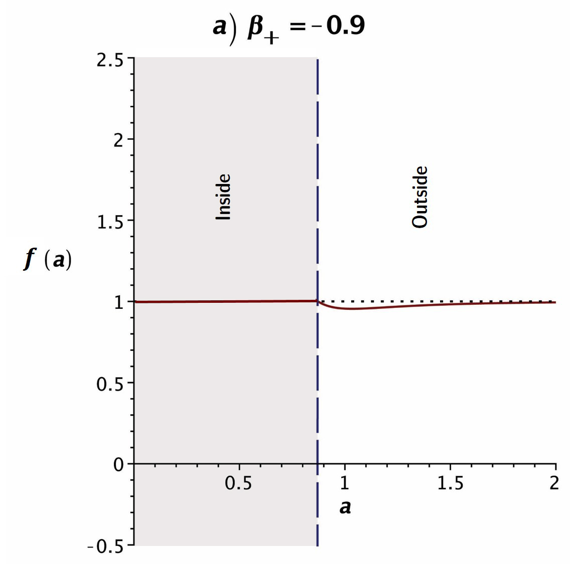
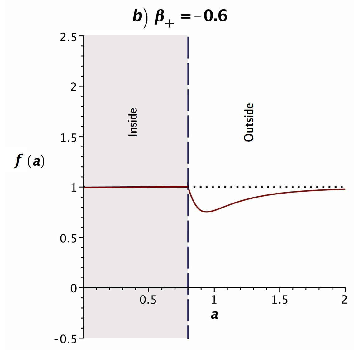
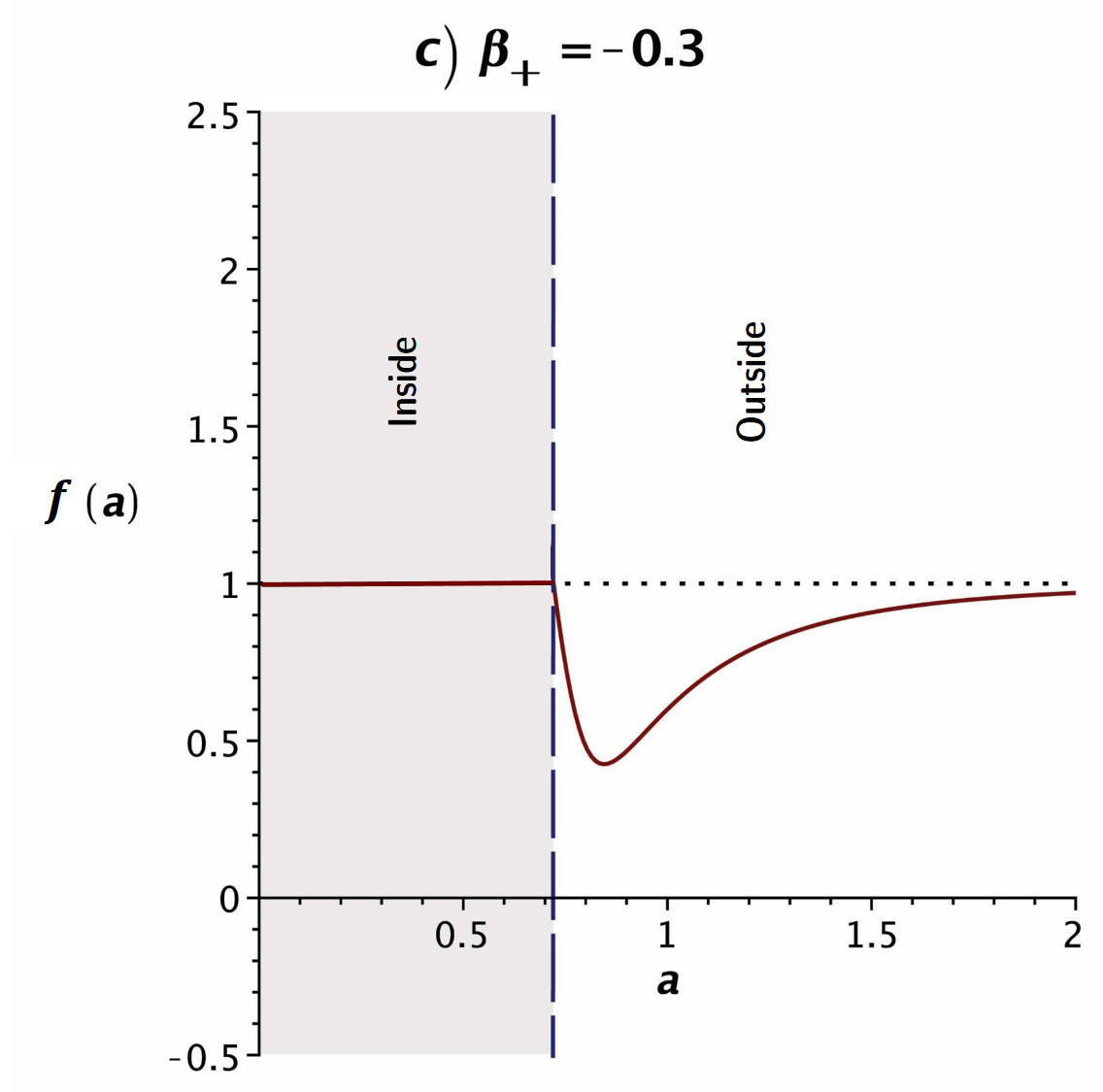
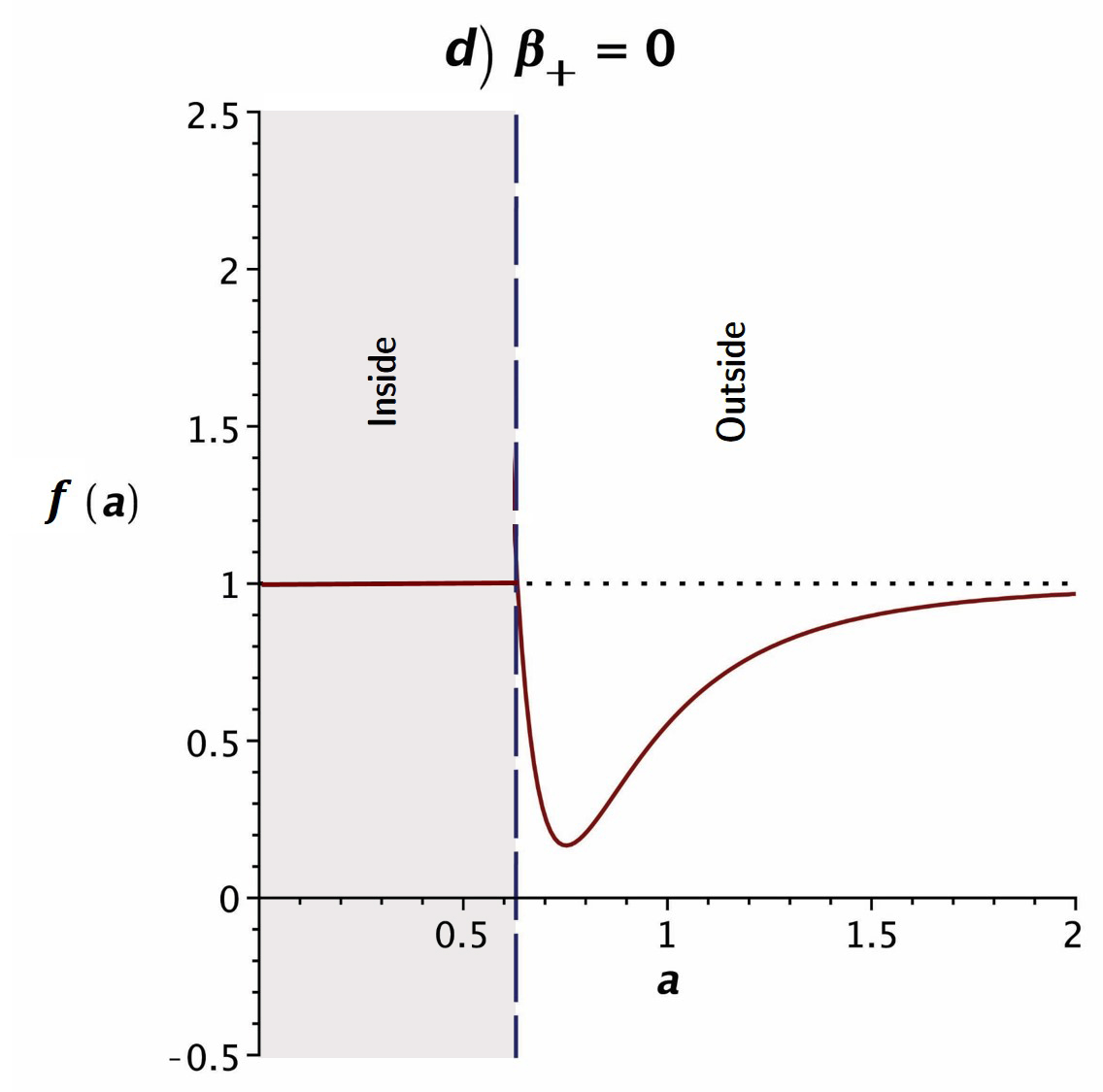
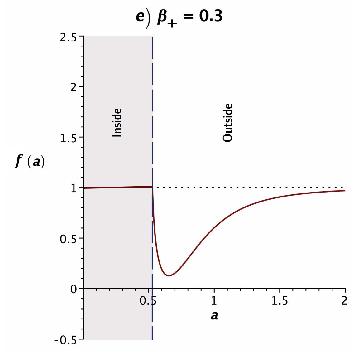
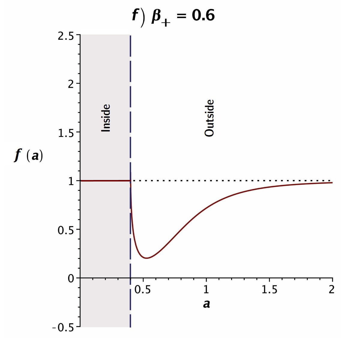
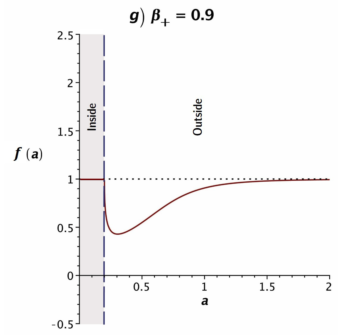
Figure 1: The graphs illustrate the metric function $f\left(a\right)$ ($f_{+}(a)$ of the exterior and $f_{-}(a)=1$ of the interior spacetimes) versus the equilibrium radius $a$, for five different values of $\beta_{+}$ where $\beta_{-}=-1$. The results suggest that for the admissible domain of $\beta_{+}$ the particle model is feasible. The vertical line is the location of the particle’s radius.

Here are some remarks. From Eq. (18) it is evident that the charge $q$ is zero when $3\tilde{\alpha}_{3-}=\beta_{+}^{2}$ (or either when $\beta_{-}=\beta_{+}$ or $\beta_{-}=-\beta_{+}$ in Eq. (20)). However, these choices are banned since they also lead to a null mass (and a null equilibrium radius in the latter case). Consequently, at least for $n=6$ and the particular solution that we considered here (Eq. (9)), the existence of the Maxwell Lagrangian in the action is essential. In other words, for $n=6$ and the metric function in Eq. (9) as the exterior region, the charge must be non-zero. Let us also note that we narrowed down our degrees of freedom by choosing the special case $\tilde{\alpha}_{2+}^{2}=3\tilde{\alpha}_{3+}=\beta_{+}^{2}$ and $n=6$. Moreover, here we illustrated in Fig. 1 only the metric functions of a particle for which $f_{-}=f_{+}$, $\tilde{\alpha}_{2-}^{2}=3\tilde{\alpha}_{3-}=\beta_{-}^{2}$ and $\beta_{-}=-1$. It is obvious that lifting any of these conditions may result in a different particle with different radius, mass and charge.

As for the next step, let us analyze our model from a different point of view by going back to Eq. (16) and discussing it in a more physical and extensive fashion. This time, there is no constraint on the radius, and the inside coupling constants $\tilde{\alpha}_{2-}$ and $\tilde{\alpha}_{3-}$ are independent of each other. As it was mentioned before, we could have solved the system of equations $\sigma=0$ and $p=0$ to find $\tilde{\alpha}_{2-}$ and $\tilde{\alpha}_{3-}$ in terms of $m$, $q$, $a$ and $\beta_{+}$. This would result in the intricate expressions

$$\tilde{\alpha}_{2-}=\frac{1}{8\left[a^{8}+a^{6}\beta_{+}+\left(\beta_{+}^{2}/3-m\right)a^{4}+q^{2}\right]a^{2}}\times\\ \left\{\sqrt{\frac{1}{\beta_{+}}\left(-a^{2}\sqrt[3]{\frac{a^{10}+3a^{4}m\beta_{+}-3q^{2}\beta_{+}}{a^{10}}}+a^{2}+\beta_{+}\right)}\right.\;\times\\ \left[\left(2a^{12}+\beta_{+}a^{10}-2a^{4}q^{2}\right)\left(\frac{a^{10}+3a^{4}m\beta_{+}-3q^{2}\beta_{+}}{a^{10}}\right)^{2/3}\right.\\ +\left(3a^{12}+4\beta_{+}a^{10}+\left(\frac{4\beta_{+}^{2}}{3}-m\right)a^{8}-a^{4}q^{2}-2a^{2}q^{2}\beta_{+}\right)\sqrt[3]{\frac{a^{10}+3a^{4}m\beta_{+}-3q^{2}\beta_{+}}{a^{10}}}\\ \left.+\left(7a^{10}+8a^{8}\beta_{+}+\left(\frac{8\beta_{+}^{2}}{3}-5m\right)a^{6}+3a^{2}q^{2}-2q^{2}\beta_{+}\right)\left(a^{2}+\beta_{+}\right)\right]\\ \left.-12\left(a^{8}+a^{6}\beta_{+}+\left(\frac{\beta_{+}^{2}}{3}-m\right)a^{4}+q^{2}\right)a^{4}\right\}$$ (23)

and

$$\tilde{\alpha}_{3-}=\frac{1}{38\left[a^{8}+a^{6}\beta_{+}+\left(\beta_{+}^{2}/3-m\right)a^{4}+q^{2}\right]}\times\\ \left\{\sqrt{\frac{1}{\beta_{+}}\left(-a^{2}\sqrt[3]{\frac{a^{10}+3a^{4}m\beta_{+}-3q^{2}\beta_{+}}{a^{10}}}+a^{2}+\beta_{+}\right)}\right.\;\times\\ \left[\left(-4a^{12}+\beta_{+}a^{10}+6\left(\frac{\beta_{+}^{2}}{3}-m\right)a^{8}+16a^{4}q^{2}\right)\left(\frac{a^{10}+3a^{4}m\beta_{+}-3q^{2}\beta_{+}}{a^{10}}\right)^{2/3}\right.\\ +\left(-7a^{12}-4\beta_{+}a^{10}+3\left(\frac{4\beta_{+}^{2}}{3}-m\right)a^{8}+8\beta_{+}\left(\frac{\beta_{+}^{2}}{3}-m\right)a^{6}+13a^{4}q^{2}+18a^{2}q^{2}\beta_{+}\right)\sqrt[3]{\frac{a^{10}+3a^{4}m\beta_{+}-3q^{2}\beta_{+}}{a^{10}}}\\ \left.-\left(19a^{10}+8a^{8}\beta_{+}+3\left(-\frac{8\beta_{+}^{2}}{3}-3m\right)a^{6}+16\beta_{+}\left(-\frac{\beta_{+}^{2}}{3}+m\right)a^{4}-a^{2}q^{2}-26q^{2}\beta_{+}\right)\left(a^{2}+\beta_{+}\right)\right]\\ \left.+30\left(a^{8}+a^{6}\beta_{+}+\left(\frac{\beta_{+}^{2}}{3}-m\right)a^{4}+q^{2}\right)a^{4}\right\}.$$ (24)

In this structure, one may use the actual data of real charged spinless particles, such as electron or proton, to find these coupling constants for each of these particles.

IV Conclusion

In a satisfactory classical geometric description of a particle, the physical properties are expressible in terms of the parameters of the theory without implementing quantum mechanics. For a charged spherical model, for instance in $3+1$ dimensions, the mass $m$ and the charge $q$ are constrained to satisfy the condition $a=$radius$\sim q^{2}/m$. In search for an analogous model in higher dimensions, we employ the TOLG as a useful theory, in the first part of the article. The reason for this choice relies on the existence of enough free parameters to define the particle properties. The existence of exact solutions, suitable to define thin, spherical shells, provides enough motivating factors towards construction of a particle model. For $n+1$ dimensions ($n\geq 6$), we consider a spherical shell, as representative of a particle, whose inside is a flat vacuum, with no electric field, to be connected through the proper junction conditions to a curved, asymptotically flat outside region. In the process, to have a particle model, the emergent fluid’s energy-momentum components on the shell (which is now the particle’s surface) are required to vanish. This yields the mass and the charge of the particle in terms of the parameters of the theory, which are to be tuned-finely. The dimensionality naturally reflects in the radius of the particle, i.e. $a=\left(q^{2}/m\right)^{1/\left(n-2\right)}$. In classical physics, to get the classical radius of a charged particle both inside and outside of the particle are flat. In the present model this assumptions holds true no more, yet, the radius has a good agreement with the classical model. Therefore, Eq. (17) can be looked at as a higher-dimensional equivalent for the classical charged particle radius.

We finally remark that in our model of particle spin is absent. This can be taken into consideration with the extension of the thin-shell formalism and diagonal Lovelock metrics to stationary forms.

V Acknowledgment

SDF would like to thank the Department of Physics at Eastern Mediterranean University, specially the chairman of the department, Prof. İzzet Sakallı for the extended facilities.

References

• (1) A. V. Vilenkin, and P. I. Fomin, ITP Report No. ITP-74-78R (1974).
• (2) A. V. Vilenkin, and P. I. Fomin, Nuovo Cimento Soc. Ital. Fis. A 45, 59 (1978).
• (3) J. A. Wheeler, Geometrodynamics (Academic Press, the University of California, 1962).
• (4) B. Bertotti, Phys. Rev. 116, 1331 (1959).
• (5) I. Robinson, Bull. Acad. Pol. Sci. 7, 351 (1959).
• (6) O. B. Zaslavskii, Phys. Rev. D 70, 104017 (2004).
• (7) D. Lovelock, J. Math. Phys. 12, 498 (1971).
• (8) G. D. Birkhoff, Relativity and Modern Physics (Cambridge, Massachusetts: Harvard University Press. 1923, LCCN 23008297),
• (9) Z. Amirabi, Phys. Rev. D 88, 087503 (2013).
• (10) M. R. Mehdizadeh, M. Kord Zangeneh, and F. S. N. Lobo, Phys. Rev. D 92, 044022 (2015).
• (11) G. Darmois, Mémorial de Sciences Mathématiques, 25 (1927).
• (12) W. Israel, Thin shells in general relativity, II Nuovo Cim. 66 (1966) 1.
• (13) M. H. Dehghani, and R. B. Mann, Phys. Rev. D 73, 104003 (2006).
• (14) M. H. Dehghani, N. Bostani, and A. Sheykhi, Phys. Rev. D 73, 104013 (2006).
• (15) M. H. Dehghani, and M. R. Mehdizadeh, Phys. Rev. D 85, 024024 (2012).