Feature Learning Viewpoint of AdaBoost and a New Algorithm

Abstract

The AdaBoost algorithm has the superiority of resisting overfitting. Understanding the mysteries of this phenomena is a very fascinating fundamental theoretical problem. Many studies are devoted to explaining it from statistical view and margin theory. In this paper, we illustrate it from feature learning viewpoint, and propose the AdaBoost+SVM algorithm, which can explain the resistant to overfitting of AdaBoost directly and easily to understand. Firstly, we adopt the AdaBoost algorithm to learn the base classifiers. Then, instead of directly weighted combination the base classifiers, we regard them as features and input them to SVM classifier. With this, the new coefficient and bias can be obtained, which can be used to construct the final classifier. We explain the rationality of this and illustrate the theorem that when the dimension of these features increases, the performance of SVM would not be worse, which can explain the resistant to overfitting of AdaBoost.

I Introduction

The Adaboost algorithm [1, 2], which learns a “strong” classifier by voting the weighted predictions of a set of “weak” learners (slightly better than random guessing) [3], is one of the most influential classification algorithms [4, 5, 6]. The excellent performance has been demonstrated both on benchmark datasets and real application[7, 8, 9, 4, 10].

According to Occam’s razor [11], when a classifier was trained too complex, the performance of it would be even worse rather than better. This phenomena is called overfitting, which means that the trained model is so adaptable to the training data that it would exaggerate the slight fluctuations in the training data, leading to poor generalization performance[12, 4]. However, the AdaBoost algorithm has the superiority of resisting overfitting, which has been observed by many researches[13, 14, 15]. Understanding the mysteries of this phenomena about AdaBoost algorithm is a fascinating fundamental theoretical problem[12, 4]. Many studies are devoted to explaining the success of AdaBoost, which can be divided into statistical view and margin theory[16].

In the statistical view, great efforts were made to illustrate the success of AdaBoost algorithm. Friedman et al. [17] utilized the well-known statistical principles, additive modeling and maximum likelihood, to understand this mysterious phenomenon. Besides, many boosting-style algorithms were proposed with optimizing the potential loss functions in a gradient decent way[18, 19, 4]. Inspired by this optimal method, some boosting-style algorithms and their variants that were consistent to Bayes’s under different conditions were presented. [20, 21, 22, 23, 24, 25, 4, 26]. However, the biggest problem of the statistical view is that these algorithms do not explain well why AdaBoost is resistant to overfitting[12, 4].

The margin theory is another direction to solve this problem. Schapire et al.[27] were the first ones to use the margin theory to explain this overfitting phenomenon. Generally speaking, the margin of an example associated with the classifier is a measuring standard of the classification ability[10]. Schapire et al.[27] demonstrated that AdaBoost model can produce a good margin distribution which is the key to the success of AdaBoost. Soon after that, Breiman [28] put a doubt on this margin explanation. He proposed a boosting-type algorithm named arc-gv which directly maximizes the minimum margin for the generalization error of a voting classifier. In experiments, arc-gv can generate a larger minimum margin than AdaBoost, but it brought higher generalization error. Breiman concluded that neither the margin distribution nor the minimum margin has influence to the generalization error. Later, Reyzin and Schapire[3] found that, amazingly, Breiman had not controlled model complexity well in the experiments. They repeated Brieman s experiments using decision stumps with two leaves. The results showed that arc-gv was with larger minimum margin, but worse margin distribution. Therefore, a convincing explanation is urgently needed[10].

To support the margin theory, Wang et al. [29] proved a bound in terms of a new margin measure called the Equilibrium margin (Emargin). The Emargin bound was uniformly sharper than Breiman s minimum margin bound. The results suggested that the minimum margin may be not crucial for the generalization error and a small empirical error at Emargin implied a smaller bound of the generalization error. Gao and Zhou [4]. proposed the $k$th margin bound to defend the margin theory against Breiman’s doubt by a series mathematical derivation. This model was uniformly tighter than Breiman s as well as Schapire s bounds and considered the same factors as Schapire et al. and Breiman. Zhou et al. [12] proposed the Large margin Distribution Machine (LDM) to achieve a better generalization performance by optimizing the margin distribution. The margin distribution was characterized by the first-order statistic margin mean and second-order statistic variance. Then, the margin mean was tried to be maximum. At the same time, the margin variance was tried to be minimum. This method realized satisfactory results. However, completely explaining AdaBoost’s resistance to overfitting is still difficult.

In this paper, we illustrate the resistant overfitting phenomena of AdaBoost from feature learning viewpoint and using the SVM classifier to explain it. SVM classifier is very useful for its clear principles and competitive accuracy[30][31][32][33][34][35][36][37]. We regard the results of base classifiers of AdaBoost as features and input them to SVM and explain the rationality of doing this. This means when the iterations of AdaBoost increase, the features’ dimension increases. We illustrate that the margin of SVM (not the margin of AdaBoost itself) will not be smaller when the features’ dimension increase. This implies that the performance of our AdaBoost+SVM model will improve when the iterations increase, which can directly and easily explain the resistant overfitting phenomena of AdaBoost rather than the complex proof. By the way, we also illustrate that the error rate of a binary classifier is always not bigger than 0.5, which is not noticed by other researchers.

The rest of this paper is organized as follows. In Section II, we have a briefly survey on the related work of the AdaBoost Algorithm. In Section III, we present our AdaBoost+SVM model. In Section IV, we validate our methods on different datasets. In Section V, we come to a conclusion.

II Related work

In this section, we briefly review the general AdaBoost algorithm and the popular theoretical explanation to AdaBoost from the view of margin theory.

II-A AdaBoost Algorithm

AdaBoost algorithm[1] is one of boosting classification algorithms which can boost a group of weak classifiers to a strong classifier. These algorithms usually first use a base classify algorithm whose classification ability is just better than random guessing to train a base classifier from the initial training samples. Then adjust the sample weight according to the result of the base classifier, which makes the samples that was classified incorrectly be paid more attention to. And then use the adjusted samples to train a next base learner. After iterations, weighted are added to these base learners to form the final classifier. Next is the description of AdaBoost algorithm.

Let $\bm{S}=\{(x_{1},y_{1}),\cdots,(x_{i},y_{i}),\cdots,(x_{n},y_{n})\}$ denote the training samples set in the binary classification situation. $x_{i}\in\bm{X}\subseteq\mathbb{R}^{n}$ is the $i$th instance. $y_{i}\in\bm{Y}=\{-1,+1\}$ is the class label associated with $x_{i}$. AdaBoost algorithm is based on the additive model, which is the linear combination of the base classifiers $h_{t}(x)$:

$$f(x)=\sum_{t=1}^{T}\alpha_{t}h_{t}(x),$$ (1)

where $t=\{1,\cdots,T\}$ denotes the iteration number, $h_{t}(x)$ are the base classifiers trained from base classification algorithm $\mathfrak{L}$ whose classified ability is just better than random guessing and $\alpha_{t}$ are the weight coefficients.

In Eq.(1), $h_{t}(x)$ are learned from base classification algorithm $\mathfrak{L}$ based on the training sample with weight vector $D_{t}$ at $t$ iteration.

$$h_{t}(x):\bm{X}\rightarrow\{-1,+1\}.$$ (2)

Algorithm 1 AdaBoost algorithm

  Input:  Training set $S=\{(x_{1},y_{1}),(x_{2},y_{2}),\cdots,(x_{n},y_{n})\}$;   Base classification algorithm $\mathfrak{L}$ ;   Number of learning rounds $T$.Initialize sample weight vector $D_{1}=(\underbrace{\frac{1}{n},\cdots,\frac{1}{n},\cdots,\frac{1}{n}}_{n})$ for $t=1,\cdots,T$:

• Using the base classification algorithm $\mathfrak{L}$ and current weight $D_{t}$ to learn the base classifier $h_{t}(x)$ by minimizing the classification error $\epsilon_{t}$ defined in Eq. (6);

• Calculating the coefficient $\alpha_{t}$ based on Eq. (7);

• Updating the weight $D_{t+1}$ by Eq. (4);

endCombining the obtained $h_{t}(x)$ according to Eq. (10) to complete the final classifier.

  Output:  The final classifier $F(x)$.

The weight vector $D_{t}$ denotes the weight of each instance in $S$ at $t$ iteration. $D_{1}$ is composed as

$$D_{1}(i)=\frac{1}{n},i=1,2,\cdots,n,$$ (3)

and $D_{t+1}$ are composed as

$$D_{t+1}(i)=\frac{D_{t}(i)}{Z_{t}}\exp(-\alpha_{t}y_{i}h_{t}(x_{i})),i=1,2,\cdots,n,$$ (4)

where $Z_{t}$ are the normalization factors and are calculated as

$${Z_{t}}=\sum_{i=1}^{n}D_{t}(i)\exp(-\alpha_{t}y_{i}h_{t}(x_{i})).$$ (5)

From Eq.(4) and Eq.(5) we know that $D_{t+1}$ are adjusted from $D_{t}$. Thus the samples which are classified incorrectly in $h_{t}(x)$ will have higher weights in $t+1$ iteration.

Given training set $S$ and sample weight $D_{t}$, the object of $h_{t}(x)$ is to minimizing the classification error $\epsilon_{t}$. $\epsilon_{t}$ is calculated as

$$\epsilon_{t}=P[h_{t}(x_{i})\neq y_{i}]=\sum_{i=1}^{n}D_{t}(i)I[h_{t}(x_{i})\neq y_{i}],$$ (6)

where $P[\cdot]$ denote the probability and $I[\cdot]$ denote the logic value.

In Eq.(1), $\alpha_{t}$ measure the importance of $h_{t}(x)$ in the final classifier and are calculated in the following way.

$$\alpha_{t}=\frac{1}{2}\ln(\frac{1-\epsilon_{t}}{\epsilon_{t}}).$$ (7)

From Eq.(6) and Eq.(7) we can know that when $\epsilon_{t}<0.5$ , $\alpha_{t}>0$ . And $\alpha_{t}$ would increase with $\epsilon_{t}$ decrease. In fact, AdaBoost minimizes the exponential loss function in this process[17].

We can also notice that in AdaBoost algorithm, $\epsilon_{t}$ must smaller than 0.5 . In this condition, we make a remark which is not be noticed by others as follow:

Remark. The error rate of a binary classifier is always not bigger than 0.5 .

Explanation. For binary classification problems, if the error rate $\epsilon$ of weak classifier

$$h\left(x\right)=\left\{\begin{matrix}1&x\in\Omega\\ -1&x\notin\Omega\\ \end{matrix}\right.$$ (8)

is bigger than 0.5, we can use the classifier

$$h_{c}\left(x\right)=\left\{\begin{matrix}-1&x\in\Omega\\ 1&x\notin\Omega\\ \end{matrix}\right.$$ (9)

to replace $h(x)$, which makes the error rate $\epsilon_{c}$ convert to $1-\epsilon$. Then the $\epsilon_{c}$ is smaller than 0.5 .

This remark illustrates that $\epsilon_{t}$ would always be smaller than 0.5 unless equal to 0.5 . But it is almost impossible that the error rate of a classifier happens to be 0.5 .

After continuous iteration, the final classifier is

$$F(x)=sign(f(x))=sign(\sum_{t=1}^{T}\alpha_{t}h_{t}(x)).$$ (10)

This algorithm is summarized in Algorithm 1.

II-B Intuition of the Margin Theory

AdaBoost is one of the most influential and successful classification algorithms. However, the mystery of the phenomenon of its resistant overfitting attracted many scholars working on it. A theory which is intuitive to explain this phenomenon is the margin theroy. That is although the training error reaches zero, the margin of AdaBoost will increases along with the iterations increase.

Schapire et al.[27] were the first ones to use the margin theory to explain this overfitting phenomenon. Define $yf(x)$ as the margin for $(x,y)$ with respect to $f$. Use $P_{D}[\cdot]$ to refer as the probability with respect to sample weight vector $D$, and $P_{S}[\cdot]$ to denote the probability with respect to uniform distribution over the sample $S$. They first proved the following theorem to bound the generalization error of each voting classifier:

Theorem 1 Let $S$ be a sample of $n$ examples chosen independently at random according to $D$. Assume that the base hypothesis space $\mathcal{H}$ and $\delta>0$. Then with probability at least $1-\delta$ over the random choice of the training set $S$, every weighted averange function $f\in\mathcal{C}$ satisfies the following bound for all $\theta>0$:

$$\begin{split}{{P}_{D}}&\left[yf\left(x\right)\leq 0\right]\leq{{P}_{S}}\left[yf\left(x\right)\leq\theta\right]+\\ &O\left(\frac{1}{\sqrt{n}}{{\left(\frac{\log n\log\left|\mathcal{H}\right|}{{{\theta}^{2}}}+\log\frac{1}{\delta}\right)}^{1/2}}\right).\end{split}$$ (11)

If $\mathcal{H}$ is finite, then

$$\begin{split}{{P}_{D}}&\left[yf\left(x\right)\leq 0\right]\leq{{P}_{S}}\left[yf\left(x\right)\leq\theta\right]+\\ &O\left(\frac{1}{\sqrt{n}}{{\left(\frac{d\log^{2}(n/d)}{{{\theta}^{2}}}+\log\frac{1}{\delta}\right)}^{1/2}}\right),\end{split}$$ (12)

where $d$ is the VC dimension of $\mathcal{H}$.

This theorem illustrates that if a voting classifier generates a good margin distribution, then the generalization error is also small.

Then they propose that if $\theta$ is not too large, the fraction of training examples for which $yf(x)\leq\theta$ decreases to zero exponentially fast with the number of base hypotheses.

Theorem 2 Suppose the base learning algorithm, when called by AdaBoost, generates hypotheses with weighted training errors $\epsilon_{1},\cdots,\epsilon_{T}$. Then for any $\theta$,

$${{P}_{S}}\left[yf\left(x\right)\leq\theta\right]\leq 2^{T}\prod_{t=1}^{T}\sqrt{\epsilon_{t}^{1-\theta}(1-\epsilon_{t})^{1+\theta}}.$$ (13)

Assume that, for all t, $\epsilon_{t}\leq 1/2-\gamma$ for some $\gamma>0$, the upper bound in Eq. 13 can simplify to:

$$\left(\sqrt{(1-2\gamma)^{1-\theta}(1+2\gamma)^{1+\theta}}\right)^{T}.$$ (14)

If $\theta<\gamma$, it is easy to find that the expression inside the parentheses is smaller than 1 so that the probability that $yf(x)<\theta$ decreases exponentially fast with $T$. That is to say with the $T$ increase, AdaBoost can provide better margin distribution, which seems to explained the resistant overfitting phenomenon. This explanation is quite intuitive.

Later, Breiman[28] proved a generalization bound, which is tighter than Eq.(11) and designed the arc-gv algorithm which directly maximizes the minimum margin. According to margin theory, arc-gv should perform better than AdaBoost. However, the experiments results show that arc-gv does produce uniformly larger minimum margin but the test error increases. Thus Breiman concluded that the margin theory was in serious doubt.

Several years later, Reyzin and Schapire[3] found that Breiman had not controlled model complexity well in the experiments. They repeated Brieman s experiments using decision stumps with two leaves. The results showed that arc-gv was with larger minimum margin, but worse margin distribution. Later, Wang et al. [29] proved a bound in terms of a new margin measure called the Equilibrium margin (Emargin). The Emargin bound was uniformly sharper than Breiman s minimum margin bound. The results suggested that the minimum margin may be not crucial for the generalization error and a small empirical error at Emargin implied a smaller bound of the generalization error. Gao and Zhou [4]. proposed the $k$th margin bound to defend the margin theory against Breiman’s doubt by a series mathematical derivation. This model was uniformly tighter than Breiman s as well as Schapire s bounds and considered the same factors as Schapire et al. and Breiman. Zhou et al. [12] proposed the Large margin Distribution Machine (LDM) to achieve a better generalization performance by optimizing the margin distribution. The margin distribution was characterized by the first-order statistic margin mean and second-order statistic variance. Then, the margin mean was tried to be maximum. At the same time, the margin variance was tried to be minimum. This method realized satisfactory results. However, completely explaining AdaBoost’s resistance to overfitting is still difficult.

In fact, the certain relationship of the margin $yf(x)$ of AdaBoost itself with the iteration number $T$ is still not clearly from the works above. That is these works can not directly explain the resistant overfitting of AdaBoost when the iteration number $T$ increases even after the training error reaches $0$. In next section, we will introduce our AdaBoost+SVM model, which can give the certain relationship of iteration number $T$ and the SVM margin to explain the resistant overfitting phenomena of AdaBoost directly.

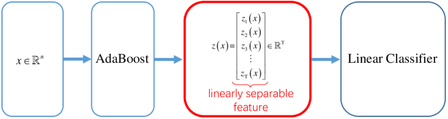
Figure 1: The feature learning view of AdaBoost.

III Feature Learning Viewpoint

In this section, we propose our AdaBoost+SVM model to explain the resistant overfitting phenomena of AdaBoost from the feature learning viewpoint and explain the rationality of doing this.

Freund and Schapire[1] have proved that the training error of AdaBoost decreases exponentially fast constantly during the learning process. There is a theorem as follows:

Theorem 3 The training error of AdaBoost will always reach $0$ since the iterations increase.

This theorem comes from the following equation:

$$\frac{1}{n}\sum\limits_{i=1}^{n}{I\left(F\left({{x}_{i}}\right)\neq{{y}_{i}}\right)}\leq\exp\left(-2\sum\limits_{t=1}^{T}{\gamma_{t}^{2}}\right),$$ (15)

where ${{\gamma}_{t}}=0.5-{{\epsilon}_{t}}$, $T$ denotes the number of iteration.

We have explained that $\epsilon_{t}$ is always smaller than 0.5 in previous chapter. Therefore $0<\gamma_{t}\leq 0.5$ .

Let $\forall{\gamma}_{t}$, $0<\gamma\leq{{\gamma}_{t}}$,

$$\frac{1}{n}\sum\limits_{i=1}^{n}{I\left(F\left({{x}_{i}}\right)\neq{{y}_{i}}\right)}\leq\exp\left(-2T{\gamma^{2}}\right).$$ (16)

Then from Eq.(16) we can easily know that the error of AdaBoost will be reduced at an exponential rate and always reach 0 when iterations are enough. Based on this theorem, we will propose our model to view AdaBoost from the feature learning point next.

III-A AdaBoost+hard margin SVM

The boosting part $\sum\limits_{t=1}^{T}{{{\alpha}_{t}}{{h}_{t}}\left(x\right)}$ in final classifier of AdaBoost given in equal (10) can be rewritten as

$$f\left(x\right)=\left[{{\alpha}_{1}},{{\alpha}_{2}},\cdots,{{\alpha}_{T}}\right]\left[\begin{matrix}{{h}_{1}}\left(x\right)\\ {{h}_{2}}\left(x\right)\\ \vdots\\ {{h}_{T}}\left(x\right)\\ \end{matrix}\right].$$ (17)

In Eq.(17), we can regard the right vector

$$z(x)={{\left[{{h}_{1}}\left(x\right),{{h}_{2}}\left(x\right),\cdots,{{h}_{T}}\left(x\right)\right]}^{T}}$$ (18)

as a feature of sample $x$ that learning from AdaBoost. Then $\alpha=\left[{{\alpha}_{1}},{{\alpha}_{2}},\cdots,{{\alpha}_{T}}\right]$ is the weight vector of this feature provided by AdaBoost algorithm. In other words, we can regard the process $x\rightarrow z(x)$ as a $\mathbb{R}^{n}\rightarrow\mathbb{R}^{T}$ spatial mapping. From this view, $\alpha$ can be viewed as a hyperplane in the feature space $\mathbb{R}^{T}$ and divide the features into two categories.

However, $\alpha$ may not be the best hyperplane for classifying the features. According to Theorem 2, the training error of AdaBoost will always reach $0$. And the training error of AdaBoost reaches $0$ means the feature $z(x)\in\mathbb{R}^{T}$ can be linearly separated into two categories. Another fact is that SVM algorithm can provide the separating hyperplane with largest margin in linearly separable problem, which means an excellent solution[38]. Based on this, use SVM algorithm to calculate the hyperplane in the feature space $\mathbb{R}^{T}$ to replace $\alpha$ should be a better choice. This is the theoretical basis of our model. The algorithm will be described next.

Given the training sample $S$, get the feature function $z(x)$ by AdaBoost algorithm according to Eq.(18), first. Then, according to the following objective function of SVM:

$$\min_{\beta,b}\,\frac{1}{2}\|\beta\|^{2}$$

$$s.t.\quad y_{i}(\beta z(x_{i})+b)-1\geq 0,i=1,2,\cdots,n,$$ (19)

we can calculate the optimal weight vector $\beta$ and bias $b$. Last, the final classifier can be learned by

$$F(x)=sign(f(x))=sign(\sum_{t=1}^{T}\beta_{t}h_{t}(x)+b).$$ (20)

We illustrate the feature learning view of AdaBoost in Fig. 1.

III-B AdaBoost+soft magin SVM

Although the training error of AdaBoost will always reach 0 with the iterations growing, in practical situation, the training error may usually not reach 0 beacause of the fixed iterations or large-scale data et al. In this situation, the features from $z(x)\in\mathbb{R}^{T}$ maybe can not be linearly separated so that the hard margin SVM is not suitable. To solve this problem, we use soft margin SVM to replace the hard margin SVM, i.e. add an additional margin violation $\xi_{i}$ to Eq.(III-A). The objective function is[39]:

$$\underset{\beta,b,\xi}{\mathop{\min}}\, \frac{1}{2}{{\left\|\beta\right\|}^{2}}+C\sum\limits_{i=1}^{n}{{{\xi}_{i}}}$$

$$s.t.\ y_{i}(\beta z(x_{i})+b)\geq 1-{\xi}_{i}$$

$${\xi}_{i}\geq 0,i=1,2,\cdots,n,$$ (21)

where $C$ represents the tolerance of the margin violation $\xi_{i}$.

Then we can use this way to solve our model whether the training error of AdaBoost reachs 0 or not.

The algorithm of AdaBoost+SVM is described in Algorithm 2.

Algorithm 2 AdaBoost+SVM algorithm.

  Input:  Training sample $S$;   Base learning algorithm $\mathfrak{L}$;   Number of base learners $T$.

• Using AdaBoost to get the feature function $z(x)$

  according to Eq.(18);

• Using SVM classifier to calculate the new coefficient $\beta$ and the bias $b$ according to Eq.(III-B);

• Combining the obtained $\beta$ , $b$ and the feature function to complete the final classifier according to Eq. (20).

  Output:  The final classifier $F(x)$.

III-C The explanation to the resistant overfitting by our model

Overfitting is a common problem in many classification situation. However, the AdaBoost algorithm can resist overfitting. Understanding the mystery is a very fascinating fundamental theoretical problem. Our AdaBoost+SVM model also has the superiority of explaining this phenomenon. We utilize the following theorem to analyze this property from feature learning viewpoint.

Theorem 4  SVM is a linear classifier in the feature space. As the dimensions of features increases, the margin of SVM will not be smaller.

Proof. The objective function of SVM is:

$$\min_{\beta,b}\,\frac{1}{2}\|\beta\|^{2}$$

$$s.t.\quad y_{i}(\beta x_{i}+b)-1\geq 0,i=1,2,\cdots,n.$$ (22)

The optimal solution $\beta^{*}$ and $b^{*}$ can be calculated. Then, the corresponding hard margin separation hyperplane is

$$\beta^{*}x+b^{*}=0.$$ (23)

If $x$ increases to $(x,x_{t})$, then the corresponding $\beta$ becomes to $(\beta,\beta_{t})$. The new optimal solution $\beta_{new}^{*}$ and $b_{new}^{*}$ can be obtained. Then, the corresponding hard margin separation hyperplane is

$$\beta_{new}^{*}x+b_{new}^{*}=0.$$ (24)

If $\beta_{t}=0$, the margin will stay the same. If $\beta_{t}\neq 0$, the margin will become larger. In a word, the margin does not become smaller when the dimensions of features are increased. According to[16], the bigger margin is, the higher the predictive confidence is. Therefore, as the number of feature increases, the classification performance will not decrease.

Based on this theorem, we regard the obtained results of base classifiers by the AdaBoost algorithm as features of SVM. As the dimensions of features increases, the performance of SVM classifier would be improved, which can easily explain the advantage of AdaBoost that can resist overfitting. Therefore, our AdaBoost+SVM model have illustrated the mysteries of resistant overfitting from the feature learning viewpoint.

It should be noticed that as the number of $T$ increased, we can not directly obtain the $\theta$ in Eq.(13) also increase. But in our model, the increase of $T$ must be helpful for better performance, which can explain the resistant overfitting phenomena of AdaBoost directly and easily.

IV Experiment

In this section, we conduct experiments on four binary benchmark datasets to demonstrate the efficiency and effectiveness of the proposed method. Then, we have a detail analysis about the experimental results.

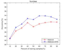
(a)

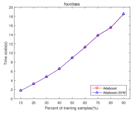
(b)

Figure 2: Classification accuracy ($\%$) and time costs vs the percent of labeled samples on fourclass dataset.

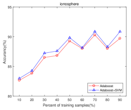
(a)

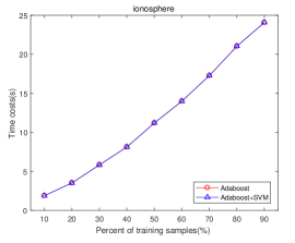
(b)

Figure 3: Classification accuracy ($\%$) and time costs vs the percent of labeled samples on ionosphere dataset.

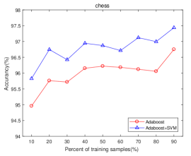
(a)

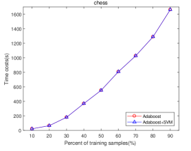
(b)

Figure 4: Classification accuracy ($\%$) and time costs vs the percent of labeled samples on chess dataset.

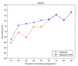
(a)

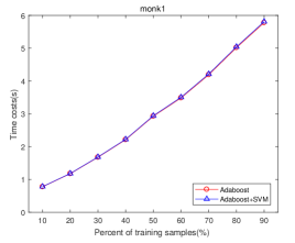
(b)

Figure 5: Classification accuracy ($\%$) and time costs vs the percent of labeled samples on monk1 dataset.

IV-A Datasets

We utilize the following $4$ binary datasets to evaluate the performance of our model.

1. fourclass: This dataset totally has $862$ samples and $2$ dimensions.

2. ionosphere: This dataset is one of the UCI dataset with $351$ samples and $34$ features.

3. chess: This dataset is also belongs to UCI dataset with $3196$ samples and $36$ features.

4. monk1: This dataset is also one of the UCI dataset with $432$ samples and $6$ features.

The detail descriptions of all datasets are also listed in Table I.

TABLE I: Dataset Description

Dataset	Samples	Features	Dataset	Samples	Features
fourclass	862	2	ionosphere	351	34
chess	3196	36	monk1	432	6

IV-B Comparison Methods

To demonstrate the effectiveness of the proposed approaches, we compare it with the classical AdaBoost algorithm. For all the methods, we run $5$ times and evaluate the classification results with the average classification accuracies and time costs. All the experiments are implemented in MATLAB R$2017$a, and run on a windows $10$ machine with a $3.6$GHz Intel i$7$-$7700$ CPU and $32$GB RAM.

TABLE II: Classification accuracy ($\%$) and time cost (s) vs the number of weak learner on fourclass dataset

Learner	Classification accuracy ($\%$)		Time cost (s)
	AdaBoost	AdaBoost+SVM	AdaBoost	AdaBoost+SVM
100	88.74	93.27	18.00	18.08
200	89.44	91.99	18.00	18.08
300	89.78	92.45	30.45	30.57
400	89.55	92.58	47.82	48.00
500	89.90	92.92	65.63	65.88
600	90.13	92.00	74.69	74.96
700	90.37	92.69	113.43	113.85
800	90.48	91.53	138.46	138.96
900	90.60	91.30	163.72	164.27
1000	89.91	90.60	194.53	195.19

TABLE III: Classification accuracy ($\%$) and time cost (s) vs the number of weak learner on ionosphere dataset

Learner	Classification accuracy ($\%$)		Time cost (s)
	AdaBoost	AdaBoost+SVM	AdaBoost	AdaBoost+SVM
100	90.88	90.89	11.34	11.35
200	91.46	90.61	24.71	24.72
300	91.74	90.60	36.10	36.12
400	91.74	90.89	47.51	47.54
500	91.17	90.89	60.66	60.69
600	90.89	90.60	87.92	87.98
700	91.45	90.32	104.49	104.56
800	90.89	90.60	120.18	120.26
900	91.45	90.32	135.99	136.08
1000	90.89	90.60	155.91	155.00

TABLE IV: Classification accuracy ($\%$) and time cost (s) vs the number of weak learner on chess dataset

Learner	Classification accuracy ($\%$)		Time cost (s)
	AdaBoost	AdaBoost+SVM	AdaBoost	AdaBoost+SVM
100	95.87	97.09	545.83	546.11
200	96.50	97.03	987.05	987.50
300	96.81	97.15	1586.54	1587.39
400	96.81	97.18	2195.24	2196.46
500	96.93	97.28	2551.54	2552.89
600	96.93	97.31	3200.47	3202.18
700	96.81	97.34	3873.00	3875.16
800	96.75	97.37	4347.55	4349.90
900	96.87	97.28	4807.12	4809.74
1000	96.84	97.34	5303.47	5306.41

TABLE V: Classification accuracy ($\%$) and time cost (s) vs the number of weak learner on monk1 dataset

Learner	Classification accuracy ($\%$)		Time cost (s)
	AdaBoost	AdaBoost+SVM	AdaBoost	AdaBoost+SVM
100	74.98	74.98	3.32	3.34
200	74.98	74.98	6.95	6.99
300	74.98	74.98	11.05	11.13
400	74.98	74.98	15.35	15.46
500	74.98	74.98	19.84	19.97
600	74.98	74.98	24.75	24.92
700	74.98	74.98	30.48	30.67
800	74.98	74.98	88.88	88.98
900	74.98	74.98	35.98	36.21
1000	74.98	74.98	41.80	42.05

IV-C The effect on the number of weak learner

In most AdaBoost algorithm, the number of weak learner is set empirically. Now, we conduct experiments on the above four binary datasets to observe the effect on the number of weak learner. We adopt the $10$-fold cross validation way [40] to select $90\%$ in each class labeled samples as the training data to construct the classifier, the rest $10\%$ samples as the testing data to evaluate the performance of this classifier. Firstly, each dataset $S$ was divided into $10$ mutually exclusive subsets of similar size, that is $S=S_{1}\bigcup S_{2}\bigcup\cdots\bigcup S_{10},S_{i}\bigcap S_{j}=\varnothing(i\neq j)$. Besides, each subset keeps the data distribution as consistent as possible. Then, the set of $9$ subsets was used as a training set, and the remaining subset as the test set in each time, which can obtain $10$ groups training and testing set. In this way, $10$ times training and testing procedures can be conducted. Finally, we can calculate the mean of $10$ times testing results.

The number of weak learner varies from $100$ to $1000$ and the corresponding classification accuracy ($\%$) and time cost (s) on the four datasets are recorded in Table II, Table III, Table IV and Table V. From Table II to Table V, we have the following observation. Firstly, on the fourclass and chess datasets, the classification accuracies obtained by AdaBoost+SVM are a little higher than AdaBoost+SVM. On the monk1 dataset, the classification accuracies calculated by the two models are exactly equal. On the ionosphere dataset, the classification accuracies obtained by AdaBoost+SVM are a little lower than AdaBoost+SVM. However, the gap between the results of AdaBoost and AdaBoost+SVM is not very large. Then, we can see that time costs obtained by AdaBoost and AdaBoost+SVM have little gap. The reason is that SVM can quickly handle classification problems. Therefore, we can conclude that our AdaBoost+SVM is very close to the AdaBoost, which can be regarded as a new explanation to the AdaBoost algorithm.

IV-D The effect on the number of training data

Next, we conduct experiments on the above datasets to observe the effect on the number of training data. For all the datasets, we fix the number of weak learner to $200$. We vary the percent of labeled samples in each class from $10\%$ to $90\%$ as the training data, the remaining samples as testing data. The results are shown in Fig. 2, Fig. 3, Fig. 4 and Fig. 5.

As a general trend, the classification accuracy and time costs increase with the number of training samples increasing on all the datasets. However, more training data brings more time to train this classifier. Then, in terms of classification accuracies and time costs on all the datasets, the results of AdaBoost and AdaBoost+SVM are still close, which verifies the performances of the two is comparable again.

V Conclusion

In this paper, we have presented an AdaBoost+SVM model from the feature learning viewpoint to explain the success of AdaBoost that can resist the overfitting problem. Instead of directly weighted combination the base classifiers calculated by AdaBoost, we regard them as the new features and input them to the SVM classifier. The iterations increase means the dimensions of features are increase, so that the performance of SVM would be improved, which can explain the resistant overfitting phenomenon of AdaBoost model in a simple way. The results on four binary datasets show that AdaBoost+SVM can produce the comparable results to the AdaBoost algorithm, which illustrates the rationality to understand the AdaBoost algorithm from the feature learning viewpoint.

References

- [1] Y. Freund and R. E. Schapire, “A decision-theoretic generalization of on-line learning and an application to boosting,” Journal of Computer and System Sciences, vol. 55, no. 1, pp. 119 – 139, 1997.
- [2] Y. Freund and S. R. E., “Experiments with a new boosting algorithm,” in Proc. 13th Int.Conf. Mach. Learn., 1996, pp. 148–156.
- [3] L. Reyzin and R. E. Schapire, “How boosting the margin can also boost classifier complexity,” in Proc. 23rd Int.Conf. Mach. Learn., 2006, pp. 753–760.
- [4] W. Gao and Z.-H. Zhou, “On the doubt about margin explanation of boosting,” Artificial Intelligence, vol. 203, pp. 1 – 18, 2013.
- [5] R. Caruana and A. Niculescu-Mizil, “An empirical comparison of supervised learning algorithms,” in Proc. 23rd Int.Conf. Mach. Learn., 2006, pp. 161–168.
- [6] X. Wu, V. Kumar, J. R. Quinlan, J. Ghosh, Q. Yang, H. Motoda, G. J. McLachlan, A. Ng, B. Liu, S. Y. Philip et al., “Top 10 algorithms in data mining,” Knowledge and information systems, vol. 14, no. 1, pp. 1–37, 2008.
- [7] E. Bauer and R. Kohavi, “An empirical comparison of voting classification algorithms: Bagging, boosting, and variants,” Machine learning, vol. 36, no. 1-2, pp. 105–139, 1999.
- [8] T. G. Dietterich, “An experimental comparison of three methods for constructing ensembles of decision trees: Bagging, boosting, and randomization,” Machine learning, vol. 40, no. 2, pp. 139–157, 2000.
- [9] P. Viola and M. Jones, “Rapid object detection using a boosted cascade of simple features,” in Proc. IEEE Conf.Comput. Vis. Pattern Recog., vol. 1, 2001, pp. I–I.
- [10] L. Wang, M. Sugiyama, C. Yang, Z.-H. Zhou, and J. Feng, “On the margin explanation of boosting algorithms.” in COLT, 2008, pp. 479–490.
- [11] A. Blumer, A. Ehrenfeucht, D. Haussler, and M. K. Warmuth, “Occam’s razor,” Information processing letters, vol. 24, no. 6, pp. 377–380, 1987.
- [12] Z.-H. Zhou, “Large margin distribution learning,” in IAPR Workshop on Artificial Neural Networks in Pattern Recognition, 2014, pp. 1–11.
- [13] L. Breiman et al., “Arcing classifier (with discussion and a rejoinder by the author),” Ann. Statist., vol. 26, no. 3, pp. 801–849, 1998.
- [14] H. Drucker and C. Cortes, “Boosting decision trees,” in Proc. Adv. Neural Inf. Process.Syst., 1996, pp. 479–485.
- [15] J. R. Quinlan et al., “Bagging, boosting, and c4. 5,” in AAAI, vol. 1, 1996, pp. 725–730.
- [16] Z.-H. Zhou, “Boosting 25 years.” CCL, 2014.
- [17] J. Friedman, T. Hastie, R. Tibshirani et al., “Additive logistic regression: a statistical view of boosting (with discussion and a rejoinder by the authors),” Ann. Statist., vol. 28, no. 2, pp. 337–407, 2000.
- [18] P. Bühlmann and B. Yu, “Boosting with the l 2 loss: regression and classification,” Journal of the American Statistical Association, vol. 98, no. 462, pp. 324–339, 2003.
- [19] L. Mason, J. Baxter, P. L. Bartlett, and M. R. Frean, “Boosting algorithms as gradient descent,” in Proc. Adv. Neural Inf. Process.Syst., 2000, pp. 512–518.
- [20] P. L. Bartlett, M. I. Jordan, and J. D. McAuliffe, “Convexity, classification, and risk bounds,” Journal of the American Statistical Association, vol. 101, no. 473, pp. 138–156, 2006.
- [21] P. L. Bartlett and M. Traskin, “Adaboost is consistent,” J. Mach. Learn. Res., vol. 8, no. Oct, pp. 2347–2368, 2007.
- [22] P. J. Bickel, Y. Ritov, and A. Zakai, “Some theory for generalized boosting algorithms,” J. Mach. Learn. Res., vol. 7, no. May, pp. 705–732, 2006.
- [23] L. Breiman, “Some infinity theory for predictor ensembles,” Technical Report 579, Statistics Dept. UCB, Tech. Rep., 2000.
- [24] W. Jiang et al., “Process consistency for adaboost,” Ann. Statist., vol. 32, no. 1, pp. 13–29, 2004.
- [25] G. Lugosi and N. Vayatis, “On the bayes-risk consistency of regularized boosting methods,” Annals of Statistics, pp. 30–55, 2004.
- [26] I. Mukherjee, C. Rudin, and R. E. Schapire, “The rate of convergence of adaboost,” J. Mach. Learn. Res., vol. 14, no. 1, pp. 2315–2347, 2013.
- [27] R. E. Schapire, Y. Freund, P. Bartlett, and W. S. Lee, “Boosting the margin: A new explanation for the effectiveness of voting methods,” Annals of statistics, pp. 1651–1686, 1998.
- [28] L. Breiman, “Prediction games and arcing algorithms,” Neural Comput., vol. 11, no. 7, pp. 1493–1517, 1999.
- [29] L. Wang, M. Sugiyama, Z. Jing, C. Yang, Z.-H. Zhou, and J. Feng, “A refined margin analysis for boosting algorithms via equilibrium margin,” Journal of Machine Learning Research, vol. 12, no. Jun, pp. 1835–1863, 2011.
- [30] C. G. Sentelle, G. C. Anagnostopoulos, and M. Georgiopoulos, “A simple method for solving the svm regularization path for semidefinite kernels,” IEEE Trans. Neural Netw. Learn. Syst., vol. 27, no. 4, pp. 709–722, April 2016.
- [31] J. Xu, Y. Y. Tang, B. Zou, Z. Xu, L. Li, and Y. Lu, “The generalization ability of online svm classification based on markov sampling,” IEEE Trans. Neural Netw. Learn. Syst., vol. 26, no. 3, pp. 628–639, March 2015.
- [32] G.-X. Yuan, C.-H. Ho, and C.-J. Lin, “Recent advances of large-scale linear classification,” Proceedings of the IEEE, vol. 100, no. 9, pp. 2584–2603, 2012.
- [33] C. Chang and C. Lin, “Libsvm-a library for support vector machines,” Classification of Variable Objects in Massive Sky Monitoring Surveys, vol. 405, 2015.
- [34] B. Schölkopf and A. J. Smola, Learning with kernels: support vector machines, regularization, optimization, and beyond. MIT press, 2002.
- [35] V. Vapnik, The nature of statistical learning theory. Springer science & business media, 2013.
- [36] T. Joachims, “Training linear svms in linear time,” in Proc.12th ACM SIGKDD Int. Conf. Knowl. Discovery Data Mining. ACM, 2006, pp. 217–226.
- [37] C. Hou, F. Nie, C. Zhang, D. Yi, and Y. Wu, “Multiple rank multi-linear svm for matrix data classification,” Pattern Recognition, vol. 47, no. 1, pp. 454–469, 2014.
- [38] X. Wu, W. Zuo, L. Lin, W. Jia, and D. Zhang, “F-svm: Combination of feature transformation and svm learning via convex relaxation,” IEEE Trans. Neural Netw. Learn. Syst., vol. 29, no. 11, pp. 5185–5199, Nov 2018.
- [39] D.-R. C. W. Y.-X. Zhou, “Support vector machine soft margin classifiers: Error analysis,” J. Mach. Learn. Res., vol. 5, no. 12, p. 1143 C1175, Apr. 2004.
- [40] R. Kohavi, “A study of cross-validation and bootstrap for accuracy estimation and model selection,” in Proceedings of the 14th International Joint Conference on Artificial Intelligence, vol. 2, 1995, pp. 1137–1143.