Electric circuits for non-Hermitian Chern insulators

Abstract

We analyze the non-Hermitian Haldane model where the spin-orbit interaction is made non-Hermitian. The Dirac mass becomes complex. We propose to realize it by an $LC$ circuit with operational amplifiers. A topological phase transition is found to occur at a critical point where the real part of the bulk spectrum is closed. The Chern number changes its value when the real part of the mass becomes zero. In the topological phase of a nanoribbon, two non-Hermitian chiral edges emerge connecting well separated conduction and valence bands. The emergence of the chiral edge states is signaled by a strong enhancement in impedance. Remarkably it is possible to observe either the left-going or right-going chiral edge by measuring the one-point impedance. Furthermore, it is also possible to distinguish them by the phase of the two-point impedance. Namely, the phase of the impedance acquires a dynamical degree of freedom in the non-Hermitian system.

Introduction: Non-Hermitian topological systems open a new field of topological physicsBender ; Bender2 ; Malzard ; Konotop ; Rako ; Gana ; Zhu ; Yao ; Jin ; Liang ; Nori ; Lieu ; UedaPRX ; Coba ; Jiang ; JPhys . They are experimentally realized in photonic systemsMark ; Scho ; Pan ; Weimann , microwave resonatorsPoli , wave guidesZeu , quantum walksRud ; Xiao and cavity systemsHoda . The winding numberKohmoto ; Fu ; Yin and the Chern numberKohmoto ; Fu are generalized to non-Hermitian systems. There are some properties not shared by the Hermitian topological systemsBender ; Bender2 ; Malzard ; Konotop ; Rako ; Gana ; Zhu ; Yao ; Jin ; Liang ; Nori ; Lieu ; UedaPRX ; Coba ; Jiang ; JPhys . For instance, the Hall conductanceChen ; Phil ; Hirs and the chiral edge conductanceWangWang are not quantized in the non-Hermitian Chern insulators although the Chern number is quantizedFu . The typical model of the Chern insulator is the Haldane model, but there is so far no extension to the non-Hermitian model in literatures. Furthermore, although there are several studies on non-Hermitian Chern insulatorsKohmoto ; Fu ; Yao2 ; Kunst ; KawabataChern , there are so far no reports on how to realize them physically.

In this paper, we propose to realize the non-Hermitian Haldane model by an electric circuit. An electric circuit is described by a circuit Laplacian. Provided it is identified with a tight-binding HamiltonianTECNature , any results obtained based on a tight-binding Hamiltonian may find corresponding phenomena in an electric circuit. Indeed, the SSH modelComPhys , grapheneComPhys ; Hel , Weyl semimetalComPhys ; Lu , nodal-line semimetalResearch ; Luo , higher-order topological phasesTECNature ; Garcia ; EzawaTEC , Chern insulatorsHofmann , non-Hermitian topological phasesEzawaLCR ; EzawaSkin and Majorana edge statesMajoTEC have been simulated by electric circuits. The edge states are observed by measuring the impedanceTECNature ; ComPhys ; Garcia ; Hel ; Hofmann ; EzawaTEC ; EzawaLCR ; EzawaSkin .

We study a non-Hermitian Haldane model on the honeycomb lattice, where the spin-orbit interaction is made non-Hermitian. It is constructed by an $LC$ circuit together with operational amplifiers as shown in Fig.1. The spin-orbit term yields complex Dirac masses at the $K$ and $K^{\prime}$ points. The chiral edge states emerge in the topological phase. They have imaginary energy. We show a topological phase transition to occur when the real part of the bulk-energy spectrum is closed. The Chern number is determined only by the real part of the Dirac mass, while the absolute value of the bulk energy does not close at the transition point. Non-Hermitian chiral edges emerge in nanoribbon geometry, which acquire pure imaginary energy at the high symmetry points. A prominent feature is that the left-going and right-going chiral edge modes are distinguished by the phase of the two-point impedance. Furthermore, it is possible to observe only one of them by a measurement of the one-point impedance.

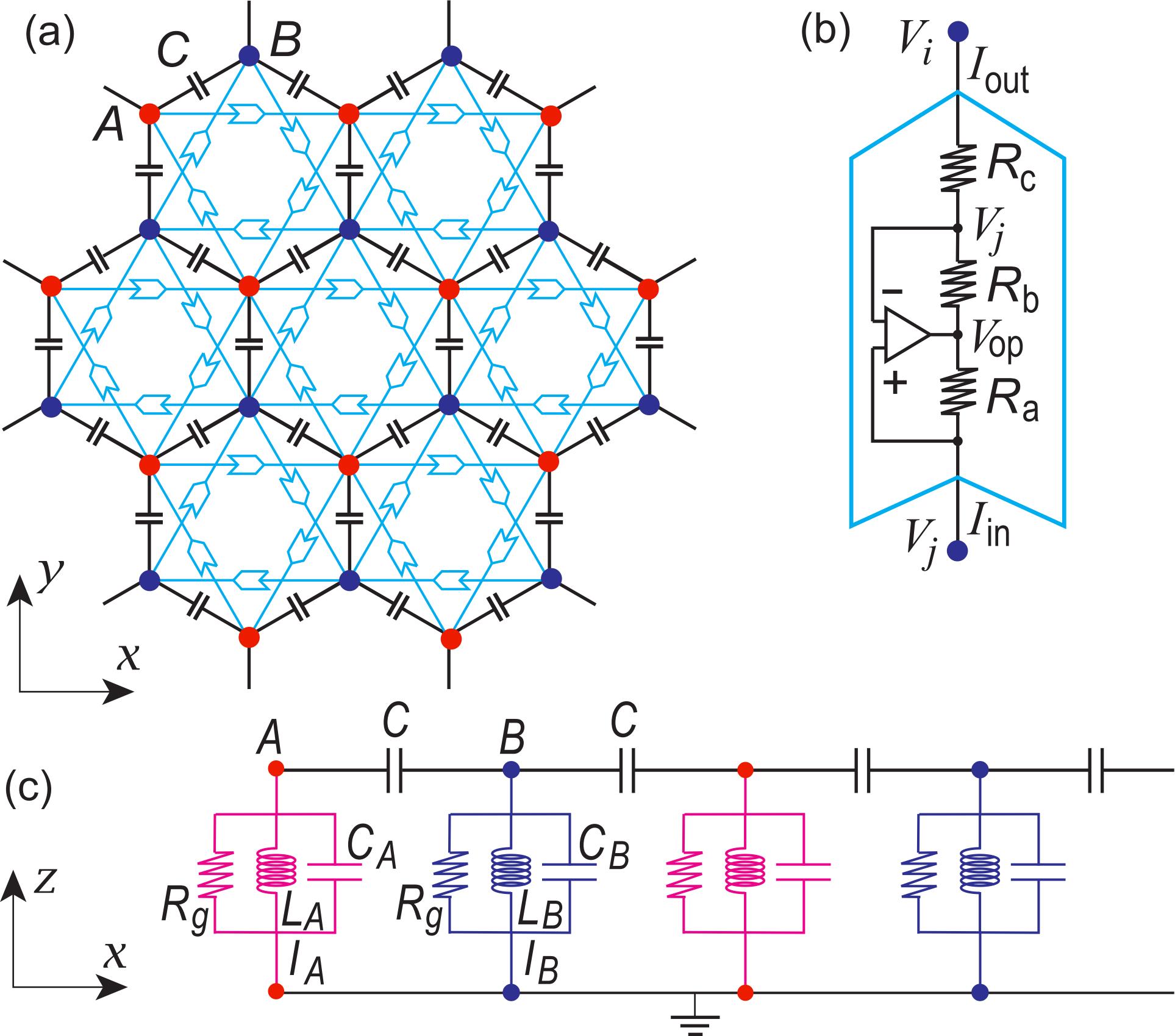
Figure 1: (a) Illustration of an electric circuit realizing the non-Hermitian Haldane model, which consists of capacitors $C$ and operational amplifiers acting as the spin-orbit interaction. (b) Structure of an operational amplifier circuitHofmann . (c) Each node is ground by a set of capacitor, inductor and resistor ($C_{A},L_{A},R_{g}$) or ($C_{B},L_{B},R_{g}$).

Non-Hermitian Haldane model: We investigate a non-Hermitian Haldane model on the honeycomb lattice, where the Haldane interaction is non-Hermitian. As described later, it is realized by an electric circuit of the configuration illustrated in Fig.1. The honeycomb lattice is a bipartite lattice, which consists of the $A$ and $B$ sites. In the basis of the $A$ and $B$ sites, the Hamiltonian is given by

$$H=\left(\begin{array}[]{cc}g\left(\boldsymbol{k}\right)+U&f\left(\boldsymbol{k}\right)\\ f^{\ast}\left(\boldsymbol{k}\right)&-g\left(\boldsymbol{k}\right)-U\end{array}\right),$$ (1)

with

$$f\left(\boldsymbol{k}\right) =t(e^{-ik_{y}/\sqrt{3}}+2e^{ik_{y}/2\sqrt{3}}\cos\frac{k_{x}}{2}),$$ (2)

$$g\left(\boldsymbol{k}\right) =\frac{i}{3\sqrt{3}}[\lambda^{r}(e^{ik_{x}}+e^{-i\frac{k_{x}+\sqrt{3}k_{y}}{2}}+e^{-i\frac{k_{x}-\sqrt{3}k_{y}}{2}})$$

$$-\lambda^{l}(e^{-ik_{x}}+e^{i\frac{k_{x}+\sqrt{3}k_{y}}{2}}+e^{i\frac{k_{x}-\sqrt{3}k_{y}}{2}})],$$ (3)

where $f\left(\boldsymbol{k}\right)$ describes hopping, and $g\left(\boldsymbol{k}\right)$ describes the non-Hermitian Haldane interaction. It is reduced to the original Haldane interaction for $\lambda^{l}=\lambda^{r}$. We have added one-site staggered potential $\pm U$, which alternates between $A$ and $B$ sites. Let us define $\lambda=\left(\lambda^{l}+\lambda^{r}\right)/2$ and $\gamma=\left(\lambda^{l}-\lambda^{r}\right)/2$, where $\gamma$ represents the non-Hermiticity.

Figure 2: Band structure of the non-Hermitian Chern insulator with zigzag nanoribbon geometry. (a1)–(c1) real part, and (a2)–(c2) imaginary part of the band structure. (a) Topological phase ($U=0$), (b) critical point ($U=\lambda$) and (c) trivial phase ($U=2\lambda$). Color represents how the wave-function localizes at the right (magenta) or left (cyan) edges. We have set $\lambda=0.2t$ and $\gamma=0.1t$.

The energy is given by $E=\pm\sqrt{\left|f\left(\boldsymbol{k}\right)\right|^{2}+\left(g\left(\boldsymbol{k}\right)+U\right)^{2}}$, which we show in Fig.2. Characteristic features read as follows. First of all, it is complex in general. The real part Re[$E$] looks very similar to the energy of the original Haldane model with $\gamma=0$, while the imaginary part Im[$E$] has peaks at the $K$ and $K^{\prime}$ points, i.e., at $\boldsymbol{K}_{\xi}=\left(\xi\frac{4\pi}{3},0\right)$ with $\xi=\pm$. The positions of the $K$ and $K^{\prime}$ points do not shift by the non-Hermitian Haldane interaction. We also show the energy spectrum in the Re[$E$]-Im[$E$] plane in Fig.3(a1)–(e1), where the conduction and valence bands are separated along the line Re[$E$]=0 except for $U=\lambda$. It is called a line gapKawabataST .

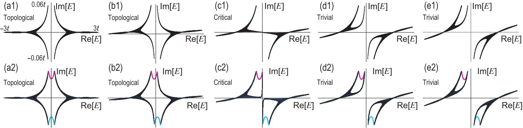
Figure 3: Energy spectrum of the non-Hermitian Chern insulator in Re$E$-Im$E$ plane (a1)–(e1) with bulk and (a2)–(e2) with zigzag nanoribbon geometry. (a1), (a2) and (b1), (b2) for topological phase ($C=1$) with $U=0$ and $U=0.5\lambda$, respectively; (c1), (c2) for critical point with $U=\lambda$; (d1), (d2) and (e1), (e2) for trivial phase ($C=0$) with $U=1.5\lambda$ and $U=2\lambda$, respectively. Magenta (cyan) color indicates the edge states localized at the right (left) edge, while black color indicates the bulk states. The edge states connect the conduction and valence bands in the topological phase, while they attach themselves to the same bands in the trivial phase. Parameters $\lambda$ and $\gamma$ are the same as in Fig.2.

We study physics near the Fermi level. We make the Taylor expansion of (2) around the $K$ and $K^{\prime}$ points. Hereafter, let us use $\boldsymbol{k}$ as the momentum measured from each of these points. We obtain $f\left(\boldsymbol{k}+\boldsymbol{K}_{\xi}\right)=\xi k_{x}-ik_{y}$ for $|\boldsymbol{k|}\ll 1$, making the Taylor expansion. Hence, the low-energy physics near the Fermi level is described by the Dirac theory,

$$H^{\xi}(\boldsymbol{k})=\hbar v_{\mathrm{F}}(\xi k_{x}\tau_{x}+k_{y}\tau_{y})+m_{\xi}\tau_{z},$$ (4)

where $v_{\text{F}}=\frac{\sqrt{3}}{2\hbar}t$ is the Fermi velocity, and

$$m_{\xi}=U-\xi\lambda-i\gamma/\sqrt{3}$$ (5)

is the Dirac masses at the $K$ and $K^{\prime}$ points.

Non-Hermitian Chern number: Since the conduction and valence bands are separated by the line gap for $U\neq\lambda$, the Chern number is well defined for $U\neq\lambda$, and characterizes the phase even in the non-Hermitian theory.

The non-Hermitian Chern number is defined byKohmoto ; Fu

$$C=\frac{1}{2\pi}\int_{\text{BZ}}F\left(\boldsymbol{k}\right)d^{2}k,$$ (6)

where $F\left(\boldsymbol{k}\right)$ is the non-Hermitian Berry curvature $F\left(\boldsymbol{k}\right)=\nabla\times A\left(\boldsymbol{k}\right)$ with the non-Hermitian Berry connectionKohmoto ; Zhu ; Yin ; Lieu $A\left(\boldsymbol{k}\right)=-i\left\langle\psi^{\text{L}}\right|\partial_{k}\left|\psi^{\text{R}}\right\rangle$. The integration of the Chern number is taken over the Brillouin zone.

We first summarize general results on the non-Hermitian Chern number in the two-band systems. We expand the Hamiltonian by the Pauli matrices, $H=\sum_{i=x,y,z}h_{i}\tau_{i}$, with $h_{i}$ being complex-valued functions. Its right and left eigenvalues are given byJiang

$$\left|\psi^{\text{R}}\right\rangle =[2E\left(E-h_{z}\right)]^{-1/2}\left(h_{x}-ih_{y},E-h_{z}\right)^{T},$$

$$\left\langle\psi^{\text{L}}\right| =[2E\left(E-h_{z}\right)]^{-1/2}\left(h_{x}+ih_{y},E-h_{z}\right),$$ (7)

which satisfy the biorthogonal condition, $\left\langle\psi^{\text{L}}\left|\psi^{\text{R}}\right\rangle\right.=1$. The non-Hermitian Berry connection is calculated asJiang

$$A_{\alpha}=(h_{x}\partial k_{k_{\alpha}}h_{y}-h_{y}\partial_{k_{\alpha}}h_{x})/[E\left(h-E\right)].$$ (8)

The non-Hermitian Berry curvature reads

$$F\left(\boldsymbol{k}\right)=2^{-1}E^{-3/2}\varepsilon_{\mu\upsilon\rho}h_{\mu}\partial_{k_{x}}h_{\nu}\partial_{k_{y}}h_{\rho}.$$ (9)

The Chern number (6) with this $F\left(\boldsymbol{k}\right)$ is understood as the Pontryagin number or the wrapping number of $h$.

For the $K$ and $K^{\prime}$ points ($\xi=\pm$) we explicitly find

$$F_{\xi}\left(\boldsymbol{k}\right)=-\frac{\xi v^{2}}{2}(m_{\xi}+U)[\left(m_{\xi}+U\right)^{2}+v^{2}k^{2}]^{-3/2}.$$ (10)

As in the case of the Hermitian systemEzawaJPSJReview , the integration of $k$ is elongated in (6) from $0$ to $\infty$ since the Berry curvature has strong peaks at the $K$ and $K^{\prime}$ points. The Chern number is

$$C_{\xi}=(m_{\xi}+U)/\left(2\sqrt{\left(m_{\xi}+U\right)^{2}}\right),$$ (11)

which is the same as in the Hermitian system although $m_{\xi}$ now takes a complex value. We find $C_{\xi}=-\xi/2$ for Re[$m_{\xi}+U$]$>0$ and $C_{\xi}=\xi/2$ for Re[$m_{\xi}+U$]$<0$, which are independent of the non-Hermiticity $\gamma$ since $\gamma$ is the imaginary part of $m_{\xi}$ as in (5). As a result, the topological phase diagram is the same as in the Hermitian model. The system is topological for $\left|\lambda\right|>\left|U\right|$ and trivial for $\left|\lambda\right|<\left|U\right|$.

Non-Hermitian chiral edge states: According to the bulk-edge correspondence in nanoribbon geometry, the topological phase is characterized by the emergence of the left-going and right-going chiral edge states which cross each other at $E=0$. An intuitive reason is that the topological number cannot change its value without gap closing. We ask how it is affected by the non-Hermitian Haldane term.

We show the energy spectra in the Re[$E$]-Im[$E$] plane in Fig.3(a2)–(e2). There are two edge states connecting the valence and conduction bands in the topological phase. On the other hand, the edge states attach themselves to the same bands in the trivial phase.

We may understand the structure as follows. In the Haldane model ($\gamma=0$), it is well known that the two chiral edges along the two edges cross at $E=0$, where $k=\pi$, charactering the topological phase ($m<\lambda$). We ask how the crossing point moves as the non-Hermiticity $\gamma$ is introduced. By perturbation theory in $\gamma$, the behavior of $E_{\text{edge}}(k)$ at $k=\pi$ is obtained analytically as $E_{\text{edge}}(\pi)=-2i\lambda\gamma$ for the $A$ sites and $E_{\text{edge}}(\pi)=2i\lambda\gamma$ for the $B$ sites. Consequently, the crossing points at $k=\pi$ become pure imaginary for $\gamma\neq 0$, as in Fig.3(a2). The bulk-band structure changes suddenly at the critical point ($m=\lambda$), resulting in the switching of the edge states between the topological and trivial phases.

Electric circuit realization: The Haldane model is constructed as in Fig.1. First, a capacitor $C$ is placed on each neighboring link of the honeycomb lattice. Second, we bridge a pair of the same type of sites by an operational amplifier, which acts as a negative impedance converter with current inversion and act as the spin-orbit interactionHofmann . Then, $A$ and $B$ sites are grounded by a set of capacitor, inductor and resistor ($C_{A},L_{A},R_{g}$) and ($C_{B},L_{B},R_{g}$), respectively.

Let us first reviewHofmann the operational amplifier when it operates in a negative feedback configuration. The current entering the operational amplifier from the bottom is given by $I_{\text{in}}=(V_{j}-V_{\text{op}})/R_{a}$, while the current leaving from the top is $I_{\text{out}}=(V_{j}-V_{i})/R_{c}$. We set an infinite impedance of the operational amplifier, where any current cannot flow into the operational amplifier. Then, the output current is given by $I_{\text{out}}=(V_{\text{op}}-V_{j})/R_{b}$. As a result, we findHofmann

$$\left(\begin{array}[]{c}I_{\text{in}}\\ I_{\text{out}}\end{array}\right)=\frac{1}{R_{c}}\left(\begin{array}[]{cc}-\nu&\nu\\ -1&1\end{array}\right)\left(\begin{array}[]{c}V_{j}\\ V_{i}\end{array}\right),$$ (12)

with $\nu=R_{b}/R_{a}$, where $R_{a}$, $R_{b}$ and $R_{c}$ are the resistances in the operational amplifier circuit: See Fig.1(b).

With the AC voltage $V\left(t\right)=V\left(0\right)e^{i\omega t}$ applied, the Kirchhoff’s current law readsComPhys ; TECNature $I_{a}\left(\omega\right)=\sum_{b}J_{ab}\left(\omega\right)V_{b}\left(\omega\right)$, where $I_{a}$ is the current between the site $a$ and the ground, while $V_{a}$ is the voltage at the site $a$. The circuit Laplacian corresponding to the circuit in Fig.1(a) is given by

$$J\left(\omega\right) =[3i\omega C+\frac{i\omega C_{A}}{2}+\frac{i\omega C_{B}}{2}-\frac{1}{2i\omega L_{A}}-\frac{1}{2i\omega L_{B}}+\frac{1}{R_{\text{g}}}]\mathbb{I}$$

$$-\left(\begin{array}[]{cc}g_{J}\left(\boldsymbol{k}\right)+U_{J}&f_{J}\left(\boldsymbol{k}\right)\\ f_{J}^{\ast}\left(\boldsymbol{k}\right)&-g_{J}\left(\boldsymbol{k}\right)-U_{J}\end{array}\right).$$ (15)

with

$$f_{J}\left(\boldsymbol{k}\right) =i\omega C\left(e^{-iak_{y}/\sqrt{3}}+2e^{iak_{y}/2\sqrt{3}}\cos\frac{ak_{x}}{2}\right)-\frac{1}{i\omega L},$$

$$g_{J}\left(\boldsymbol{k}\right) =\frac{-1}{3\sqrt{3}}[\frac{R_{b}}{R_{a}R_{c}}\left(e^{iak_{x}}+e^{-ia\frac{k_{x}+\sqrt{3}k_{y}}{2}}+e^{-ia\frac{k_{x}-\sqrt{3}k_{y}}{2}}\right)$$

$$-\frac{1}{R_{c}}\left(e^{-iak_{x}}+e^{ia\frac{k_{x}+\sqrt{3}k_{y}}{2}}+e^{ia\frac{k_{x}-\sqrt{3}k_{y}}{2}}\right)],$$

$$U =\frac{i\omega}{2}(C_{A}-C_{B})-\frac{1}{2i\omega}\left(L_{A}^{-1}-L_{B}^{-1}\right).$$ (16)

Since $J$ is a $2\times 2$ matrix, we may equate it with the Hamiltonian (1). It follows that $J=i\omega H+1/R_{\text{g}}$, provided

$$t =-C,\quad\lambda^{r}=R_{b}/(\omega R_{a}R_{c}),\quad\lambda^{l}=1/\omega R_{c},$$

$$U =-\frac{1}{2}\left(C_{A}-C_{B}\right)+\frac{1}{2\omega^{2}}\left(L_{A}^{-1}-L_{B}^{-1}\right).$$ (17)

The resistors in the operational amplifier circuit are tuned to be $\nu=1$, or $R_{a}=R_{b}$, in the literatureHofmann so that the system becomes Hermitian. However, the system is non-Hermitian for a general value of the resistors, leading to $\nu\neq 1$, which is the main theme of this paper. It is noted that the topological phase transition is induced solely controlling the capacitors $C_{A}$, $C_{B}$ or the inductors $L_{A}$, $L_{B}$ connected to the ground. We have also added resistors $R_{\text{g}}$ between nodes and the ground, whose role is shift the imaginary part of the energy.

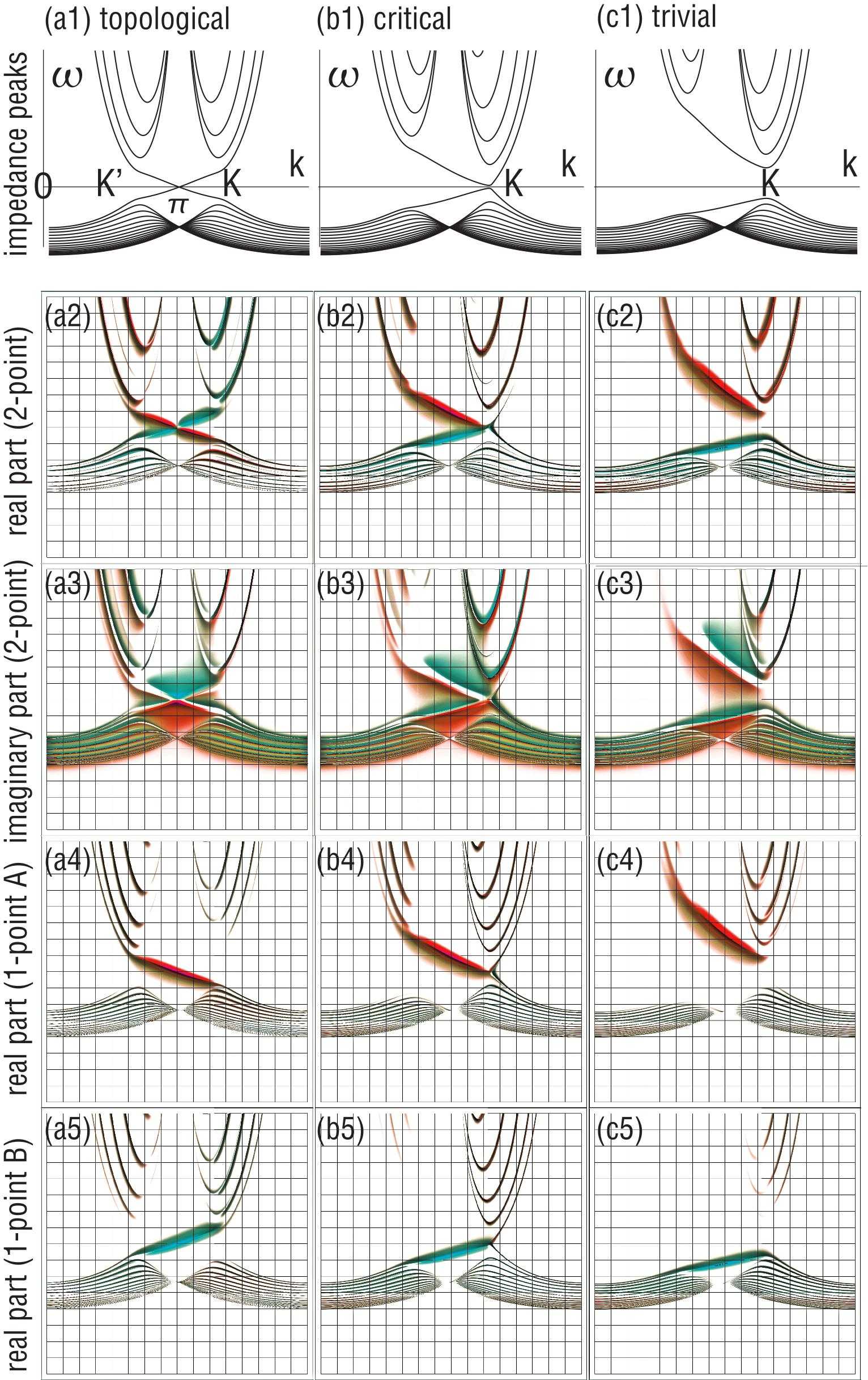
Figure 4: (a1)–(c1) Admittance curves in the $k$-$\omega$ plane given by (19), along which the impedance peaks appear. (a2)–(c2) Real part of the two-point impedance $Z_{AB}$, which is quite similar to the impedance peaks in (a1)–(c1). (a3)–(c3) Imaginary part of the two-point impedance $Z_{AB}$. (a4)–(c4) Real part of the one-point impedance $G_{A}$ at the edge at the $A$ sites. (a5)–(c5) Real part of the one-point impedance $G_{B}$ at the edge at the $B$ sites. (a) $U=0$, (b) $U=\lambda$ and (c) $U=2\lambda$. The red (green) regions indicate positive (negative) values of the impedance. We have set $\lambda=0.2t$ and $\gamma=0.1t$.

Admittance spectrum and impedance peaks: The admittance spectrum consists of the eigenvalues of the circuit LaplacianComPhys ; TECNature ; Garcia ; Hel ; Lu ; EzawaTEC (15). Indeed, it is possible to observe experimentally the admittance band structure in a direct measurementHel . It corresponds to the band structure in condensed-matter physics.

Two-point impedance is given byComPhys ; TECNature $Z_{ab}=\frac{V_{a}-V_{b}}{I_{ab}}=G_{aa}+G_{bb}-G_{ab}-G_{ba}$, where $G$ is the green function defined by the inverse of the Laplacian $J$, $G\equiv J^{-1}$. In the case of the Hermitian system, it diverges at the frequency where one of the eigenvalues of the Laplacian is zero $J_{n}=0$. Namely, the peaks of impedance are well described by the zeros of the admittance. On the other hand, in the case of the non-Hermitian system, it takes a maximum value at the frequency satisfying Re[$J_{n}$]$=0$. After the diagonalization, the circuit Laplacian yields

$$J_{n}\left(\omega\right)/i\omega = -(2\omega^{2}L_{A})^{-1}-(2\omega^{2}L_{B})^{-1}+3C$$ (18)

$$-\varepsilon_{n}\left(\omega\right)+1/i\omega R_{\text{g}},$$

where $\varepsilon_{n}$ is the eigenvalue of the corresponding Hamiltonian. It is pure imaginary for the Hermitian system but becomes complex for the non-Hermitian system. Solving Re$J_{n}\left(\omega\right)=0$, we obtain

$$\omega_{\text{R}}(\varepsilon_{n})=1/\sqrt{(-\text{Re}\left[\varepsilon_{n}\right]+3C)/\left(1/2L_{A}+1/2L_{B}\right)},$$ (19)

at which the impedance has a peak. The eigenvalue $\varepsilon_{n}$ should be solved numerically. The impedance resonance becomes weaker when the eigenvalue $\varepsilon_{n}$ has an imaginary part. However, by tuning the resistors $R_{\text{g}}$, we can decrease the imaginary part to enhance the impedance peak.

We consider a nanoribbon, where $\omega_{\text{R}}(\varepsilon_{n})$ is a function of the momentum $k_{x}$. We show it as a function of $k_{x}$ in Fig.4(a1)–(c1). The impedance has peaks at these frequencies. The impedance-peak structure in Fig.4(a1)–(c1) have some feature common to the band structure in Fig.2(a1)–(c1). The chiral edge states cross the $\omega=0$ line at $k=\pi$ when $U=0$ in Fig.4(a1). The crossing point moves towards the $K$ point as $U$ increases and reaches it when $U=\lambda$ as in Fig.4(b1). It is the signal of the topological phase. It disappears for $U>0$ as in Fig.4(c1), indicating that the system is in the trivial phase. Thus the topological phase transition induced by the potential $U$ is clearly observed in the change of the impedance peak.

We calculate the impedance with the use of Green functions as a function of $k_{x}$ and $\omega$, and show it in Fig.4(a2)–(c5), where the impedance strength is represented by darkness. Note that the momentum dependent impedance is an experimentally detectable quantityHel ; Lee by using a Fourier transformation along the nanoribbon direction,

$$Z_{\alpha\beta}\left(k_{x},y,\omega\right)=\sum_{\rho}Z_{\alpha\beta}\left(x_{\rho},y_{\rho},\omega\right)\exp\left[-ix_{\rho}k_{x}\right],$$ (20)

where $\left(x_{\rho},y_{\rho}\right)$ is the Bravais vector.

The impedance is pure imaginary in the Hermitian model. On the other hand, there emerges the real part of the impedance in the non-Hermitian model, since the energy becomes complex. It is to be emphasized that the impedance is a complex object whose real and imaginary parts are separately observable in electronics by measuring the magnitude and the phase shift of the impedance. Let us focus on the two-point impedance Re$Z_{AB}$ between the two outermost edges of a nanoribbon. It is found that the chiral edge modes become prominent as in Fig.4(a2) and (a3). This is because the imaginary part of the energy is enhanced at the $K$ and $K^{\prime}$ points. Furthermore, it is a characteristic feature of the non-Hermitian system that the left-going and right-going chiral edges are differentiated by the sign of Re$Z_{AB}$ as in Fig.4(a2), where the sign corresponds to red or green. Equivalently, they are distinguished by the phase of the impedance. This is because the imaginary part of the energy is opposite between them.

The one-point impedance is defined byHel $Z_{a}\equiv V_{a}/I_{a}=G_{aa}$. It is the inverse of the resistance between the point $a$ and the ground. The one-point impedance $Z_{A}$ at the outermost edge site $A$ is shown in Fig.4(a4)–(c4), where only the left-going chiral edge has a strong peak. It is because there is only the left-going chiral edge at the $A$ edge. On the contrary, there is a strong resonance only for the right-going chiral edge when we measure $Z_{B}$ as in Fig.4(a5)–(c5). This selective detection of the chiral edge is possible only in electric circuits.

Discussion: Topological monolayer systems such as silicene, germanene and stanene provides us with rich topological phase transitionsEzawaJPSJReview . However, their experimental realizations are yet to be made. In addition, it is hard to observe the edge states of the two dimensional topological insulators by ARPES since the intensity is very weak. On the other hand, almost all of these physics are realizable by employing electric circuits. In particular, topological phase transitions are detectable by measuring the change of impedance. Furthermore, it is possible to observe the left-going and right-going edge states separately by measuring the one-point impedance.

The author is very grateful to N. Nagaosa for helpful discussions on the subject. This work is supported by the Grants-in-Aid for Scientific Research from MEXT KAKENHI (Grants No. JP17K05490, No. JP15H05854 and No. JP18H03676). This work is also supported by CREST, JST (JPMJCR16F1 and JPMJCR1874).

References

- (1) C. M. Bender and S. Boettcher, Phys. Rev. Lett. 80, 5243 (1998).
- (2) C. M. Bender, D. C. Brody, and H. F. Jones, Phys. Rev. Lett. 89, 270401 (2002).
- (3) S. Malzard, C. Poli, H. Schomerus, Phys. Rev. Lett. 115, 200402 (2015).
- (4) V. V. Konotop, J. Yang, and D. A. Zezyulin, Rev. Mod. Phys. 88, 035002 (2016).
- (5) T. Rakovszky, J. K. Asboth, and A. Alberti, Phys. Rev. B 95, 201407(R) (2017).
- (6) R. El-Ganainy, K. G. Makris, M. Khajavikhan, Z. H. Musslimani, S. Rotter and D. N. Christodoulides, Nat. Physics 14, 11 (2018).
- (7) B. Zhu, R. Lu and S. Chen, Phys. Rev. A 89, 062102 (2014).
- (8) S. Yao and Z. Wang, Phys. Rev. Lett. 121, 086803 (2018).
- (9) L. Jin and Z. Song, Phys. Rev. B 99, 081103 (2019).
- (10) S.-D. Liang and G.-Y. Huang, Phys. Rev. A 87, 012118 (2013).
- (11) D. Leykam, K. Y. Bliokh, Chunli Huang, Y. D. Chong, and Franco Nori, Phys. Rev. Lett. 118, 040401 (2017).
- (12) S. Lieu, Phys. Rev. B 97, 045106 (2018).
- (13) Z. Gong, Y. Ashida, K. Kawabata, K. Takasan, S. Higashikawa and M. Ueda, Phys. Rev. X 8, 031079 (2018).
- (14) E. Cobanera, A. Alase, G. Ortiz, L. Viola, Phys. Rev. B 98, 245423 (2018).
- (15) H. Jiang, C. Yang and S. Chen, Phys. Rev. A 98, 052116 (2018)
- (16) A. Ghatak, T. Das, J. Phys.: Condens. Matter 31, 263001 (2019).
- (17) K. G. Makris, R. El-Ganainy, D. N. Christodoulides, and Z. H. Musslimani, Phys. Rev. Lett. 100, 103904 (2008).
- (18) H. Schomerus, Opt. Lett. 38, 1912 (2013).
- (19) M. Pan, H. Zhao, P. Miao, S. Longhi, and L. Feng, Nat. Commun. 9, 1308 (2018).
- (20) S. Weimann, M. Kremer, Y. Plotnik, Y. Lumer, S.Nolte, K. G. Makris, M. Segev, M. C. Rechtsman, and A. Szameit, Nat. Mater. 16, 433 (2017).
- (21) C. Poli, M. Bellec, U. Kuhl, F. Mortessagne and H. Schomerus, Nat. Com. 6, 6710 (2015).
- (22) J. M. Zeuner, M. C. Rechtsman, Y. Plotnik, Y. Lumer, S. Nolte, M. S. Rudner, M. Segev, and A. Szameit, Phys. Rev. Lett. 115, 040402 (2015).
- (23) M. S. Rudner and L. S. Levitov, Phys. Rev. Lett. 102, 065703 (2009).
- (24) L. Xiao, X. Zhan, Z. H. Bian, K. K. Wang, X. Zhang, X. P. Wang, J. Li, K. Mochizuki, D. Kim, N. Kawakami, W. Yi, H. Obuse, B. C. Sanders, and P. Xue, Nat. Physics 13, 1117 (2017).
- (25) H. Hodaei, A. U Hassan, S. Wittek, H. Garcia-Gracia, R. El-Ganainy, D. N. Christodoulides and M. Khajavikhan, Nature 548, 187 (2017).
- (26) K. Esaki, M. Sato, K. Hasebe, and M. Kohmoto, Phys. Rev. B 84, 205128 (2011).
- (27) H. Shen, B. Zhen and L. Fu, Phys. Rev. Lett. 120, 146402 (2018).
- (28) C. Yin, H. Jiang, L. Li, Rong Lu and S. Chen, Phys. Rev. A 97, 052115 (2018).
- (29) Y. Chen and H. Zhai, Phys. Rev. B 98, 245130 (2018).
- (30) T. M. Philip, M. R. Hirsbrunner, M. J. Gilbert, Phys. Rev. B 98, 155430 (2018).
- (31) M. R. Hirsbrunner, T. M. Philip, M. J. Gilbert, arXiv:1901.09961.
- (32) C. Wang, X. R. Wang, arXiv:1901.06982.
- (33) S. Yao, F. Song and Z. Wang, Phys. Rev. Lett. 121, 136802 (2018).
- (34) F. K. Kunst, E. Edvardsson, J. C. Budich and E. J. Bergholtz, Phys. Rev. Lett. 121, 026808 (2018).
- (35) K. Kawabata, K. Shiozaki and M. Ueda, Phys. Rev. B 98, 165148 (2018).
- (36) S. Imhof, C. Berger, F. Bayer, J. Brehm, L. Molenkamp, T. Kiessling, F. Schindler, C. H. Lee, M. Greiter, T. Neupert, R. Thomale, Nat. Phys. 14, 925 (2018).
- (37) C. H. Lee , S. Imhof, C. Berger, F. Bayer, J. Brehm, L. W. Molenkamp, T. Kiessling and R. Thomale, Communications Physics, 1, 39 (2018).
- (38) T. Helbig, T. Hofmann, C. H. Lee, R. Thomale, S. Imhof, L. W. Molenkamp and T. Kiessling, Phys. Rev. B 99, 161114 (2019).
- (39) Y. Lu, N. Jia, L. Su, C. Owens, G. Juzeliunas, D. I. Schuster and J. Simon, Phys. Rev. B 99, 020302 (2019).
- (40) K. Luo, R. Yu and H. Weng, Research (2018), ID 6793752.
- (41) K. Luo, J. Feng, Y. X. Zhao, and R. Yu, arXiv:1810.09231.
- (42) M. S.-Garcia, R. Susstrunk and S. D. Huber, Phys. Rev. B 99, 020304 (2019).
- (43) M. Ezawa, Phys. Rev. B 98, 201402(R) (2018).
- (44) T. Hofmann, T. Helbig, C. H. Lee, M. Greiter, R. Thomale, Phys. Rev. Lett. 122, 247702 (2019).
- (45) M. Ezawa, Phys. Rev. B 99, 201411(R) (2019).
- (46) M. Ezawa, Phys. Rev. B 99, 121411(R) (2019).
- (47) M. Ezawa, Phys. Rev. B 100, 045407 (2019).
- (48) K. Kawabata, K. Shiozaki, M. Ueda, M. Sato, cond-mat/arXiv:1812.09133.
- (49) M. Ezawa, J. Phys. Soc. Jpn. 84, 121003 (2015).
- (50) C. H. Lee, T. Hofmann, T. Helbig, Y. Liu, X. Zhang, M. Greiter and R. Thomale, cond-mat/arXiv:1904.10183