Deformations of Bi-conformal Energy and
a new Characterization of Quasiconformality

Abstract.

The concept of hyperelastic deformations of bi-conformal energy is developed as an extension of quasiconformality. These are homeomorphisms $\,h\colon\mathbb{X}\xrightarrow[]{{}_{\!\!\textnormal{onto\,\,}\!\!}}\mathbb{Y}\,$ between domains $\,\mathbb{X},\mathbb{Y}\subset\mathbb{R}^{n}\,$ of the Sobolev class $\,\mathscr{W}^{1,n}_{\textnormal{loc}}(\mathbb{X},\mathbb{Y})\,$ whose inverse $\,f\stackrel{{\scriptstyle\textnormal{def}}}{{=\!\!=}}h^{-1}\colon\mathbb{Y}\xrightarrow[]{{}_{\!\!\textnormal{onto\,\,}\!\!}}\mathbb{X}\,$ also belongs to $\,\mathscr{W}^{1,n}_{\textnormal{loc}}(\mathbb{Y},\mathbb{X})\,$. Thus the paper opens new topics in Geometric Function Theory (GFT) with connections to mathematical models of Nonlinear Elasticity (NE). In seeking differences and similarities with quasiconformal mappings we examine closely the modulus of continuity of deformations of bi-conformal energy. This leads us to a new characterization of quasiconformality. Specifically, it is observed that quasiconformal mappings behave locally at every point like radial stretchings. Without going into detail, if a quasiconformal map $\,h\,$ admits a function $\,\phi\,$ as its optimal modulus of continuity at a point $\,x_{\circ}\,$, then $\,f=h^{-1}\,$ admits the inverse function $\,\psi=\phi^{-1}\,$ as its modulus of continuity at $\,y_{\circ}=h(x_{\circ})\,$. That is to say; a poor (possibly harmful) continuity of $\,h\,$ at a given point $\,x_{\circ}\,$ is always compensated by a better continuity of $\,f\,$ at $\,y_{\circ}\,$, and vice versa. Such a gain/loss property, seemingly overlooked by many authors, is actually characteristic of quasiconformal mappings.

It turns out that the elastic deformations of bi-conformal energy are very different in this respect. Unexpectedly, such a map may have the same optimal modulus of continuity as its inverse deformation. In line with Hooke’s Law, when trying to restore the original shape of the body (by the inverse transformation) the modulus of continuity may neither be improved nor become worse. However, examples to confirm this phenomenon are far from being obvious; indeed, elaborate computations are on the way. We eventually hope that our examples will gain an interest in the materials science, particularly in mathematical models of hyperelasticity.

1. Introduction

We study Sobolev homeomorphisms $\,h\colon\mathbb{X}\xrightarrow[]{{}_{\!\!\textnormal{onto\,\,}\!\!}}\mathbb{Y}\,$ between domains $\,\mathbb{X},\mathbb{Y}\subset\mathbb{R}^{n}\,$, together with their inverse mappings denoted by $\,f\stackrel{{\scriptstyle\textnormal{def}}}{{=\!\!=}}h^{-1}\colon\mathbb{Y}\xrightarrow[]{{}_{\!\!\textnormal{onto\,\,}\!\!}}\mathbb{X}\,$. We impose two standing conditions on these mappings:

• The conformal energy of $\,h\,$ (stored in $\,\mathbb{X}$) is finite; that is,

  (1.1) $$\mathbf{E}_{\mathbb{X}}[h]\stackrel{{\scriptstyle\textnormal{def}}}{{=\!\!=}}\int_{\mathbb{X}}\,|Dh(x)|^{n}\,\textnormal{d}x\,<\infty$$

• The conformal energy of $\,f\,$ (stored in $\,\mathbb{Y}$) is also finite;

  (1.2) $$\mathbf{E}_{\mathbb{Y}}[f]\stackrel{{\scriptstyle\textnormal{def}}}{{=\!\!=}}\int_{\mathbb{Y}}\,|Df(y)|^{n}\,\textnormal{d}y\,<\infty$$

Hereafter, $\lvert A\rvert$ stands for the Hilbert-Schmidt norm of a linear map $A$, defined by the rule $\lvert A\rvert^{2}=\textnormal{Tr}\,(A^{t}A)$. It should be noted that the above energy integrals are invariant under conformal change of variables in their domains of definition ($\,\mathbb{X}\,$ and $\,\mathbb{Y}\,$, respectively). This motivates us calling such homeomorphisms

Deformations of Bi-conformal Energy

Clearly, such deformations include quasiconformal mappings. A Sobolev homeomorphisms $\,h\colon\mathbb{X}\xrightarrow[]{{}_{\!\!\textnormal{onto\,\,}\!\!}}\mathbb{Y}\,$ is said to be a quasiconformal mapping if there exists a constant ${\bf K}$ such that

(1.3) $$\lvert Dh(x)\rvert^{n}\leqslant{\bf K}J(x,h)\,,\qquad J(x,h)=\det Dh(x)\,.$$

The conformal energy integral (1.1), an $n$-dimensional alternative to the classical Dirichlet integral, has drawn the attention of researchers in the multidimensional GFT [7, 19, 20, 27, 46, 47, 51]. In Geometric Analysis the Sobolev space $\,\mathscr{W}^{1,n}(\mathbb{X},\mathbb{R}^{n})\,$ plays a special role for several reasons. First, this space is on the edge of the continuity properties of Sobolev’s mappings. Second, just the fact that $\,h\,$ is a homeomorphism allows us to establish uniform bounds of its modulus of continuity. Precisely, given a compact subset $\,\mathbf{X}\Subset\mathbb{X}\,$, there exists a constant $\,C(\mathbf{X},\mathbb{X})\,$ so that for all distinct points $\;x_{1},x_{2}\,\in\mathbf{X}\,$, we have:

(1.4) $$|\,h(x_{1})-h(x_{2})\,|\;\leqslant\frac{C(\mathbf{X},\mathbb{X})\;\sqrt[n]{\mathbf{E}_{\mathbb{X}}[h]}}{\log^{\frac{1}{n}}\left(1\,+\,\frac{\textnormal{diam}\,\mathbf{X}}{|x_{1}-x_{2}|}\right)}$$

For a historical account and more details concerning this estimate we refer the reader to Section 7.4, Section 7.5 and Corollary 7.5.1 in the monograph [27].

For the same reasons, to every compact $\,\mathbf{Y}\Subset\mathbb{Y}\,$ there corresponds a constant $\,C(\mathbf{Y},\mathbb{Y})\,$ such that for all distinct points $\;y_{1},y_{2}\,\in\mathbf{Y}\,$, we have:

(1.5) $$|\,f(y_{1})-f(y_{2})\,|\;\leqslant\frac{C(\mathbf{Y},\mathbb{Y})\;\sqrt[n]{\mathbf{E}_{\mathbb{Y}}[f]}}{\log^{\frac{1}{n}}\left(1\,+\,\frac{\textnormal{diam}\,\mathbf{Y}}{|y_{1}-y_{2}|}\right)}$$

In other words, $\,h\,$ and $\,f\,$ admit the same function $\,\omega=\omega(t)\approx\log^{-\frac{1}{n}}\left(1+1/t\right)\,$ as a modulus of continuity. Shortly, $\,h\,$ and $\,f\,$ are $\,\omega$-continuous. There is still a slight improvement to these estimates; namely,

(1.6) $$\lim_{|x_{1}-x_{2}|\rightarrow 0}|\,h(x_{1})-h(x_{2})\,|\,\log^{\frac{1}{n}}\left(1\,+\,\frac{\textnormal{diam}\,\mathbf{X}}{|x_{1}-x_{2}|}\right)\;=\;0$$

The question whether the modulus of continuity $\,\omega=\omega(t)\approx\log^{-\frac{1}{n}}\left(1+1/t\right)\,$ is the best and universal for all bi-conformal energy mappings remains unclear. We shall not enter this issue here. The optimal modulus of continuity of $h\colon\mathbb{X}\xrightarrow[]{{}_{\!\!\textnormal{onto\,\,}\!\!}}\mathbb{Y}$ at a given point $x_{\circ}\in\mathbb{X}$ is defined by

(1.7) $$\omega_{h}(x_{\circ};t)\stackrel{{\scriptstyle\textnormal{def}}}{{=\!\!=}}\max_{\lvert x-x_{\circ}\rvert=t}\lvert h(x)-h(x_{\circ})\rvert\qquad\textnormal{for }0\leqslant t<\operatorname{dist}(x_{\circ},\partial\mathbb{X})\,.$$

Nevertheless, it is easy to see, via examples of radial stretchings, that in the class of functions that are powers of logarithms the exponent $\,\alpha=\frac{1}{n}\,$ is sharp; meaning that for $\,\alpha>\frac{1}{n}\,$ it is not generally true that

(1.8) $$|\,h(x_{1})\,-\,h(x_{2})\,|\;\preccurlyeq\;\log^{-\alpha}\left(1\,+\,\frac{\textnormal{diam}\,\mathbf{X}}{|x_{1}-x_{2}|}\right)\;\;$$

To this end, we take a quick look at the radial homeomorphism $\,h\colon\mathbb{B}^{n}\xrightarrow[]{{}_{\!\!\textnormal{onto\,\,}\!\!}}\mathbb{B}^{n}\,$ of the unit ball $\,\mathbb{B}^{n}\subset\mathbb{R}^{n}\,$ onto itself,

(1.9) $$h(x)=\frac{x}{|x|\,\big{(}1-\log|x|\big{)}^{\frac{1}{n}}\;\big{[}\,\log(e-\log|x|)\,\big{]}^{\beta}}\;\;,\;\;\textnormal{where}\;\;\;\beta>\frac{1}{n}$$

It is often seen that the inverse map $\,f\stackrel{{\scriptstyle\textnormal{def}}}{{=\!\!=}}h^{-1}\colon\mathbb{Y}\rightarrow\mathbb{X}\,$ admits better modulus of continuity than $\,h\,$, or vice versa. Just for $\,h\,$ defined in (1.9), its inverse is even $\,\mathscr{C}^{\infty}\,$-smooth. Such a gain/loss rule about the moduli of continuity for a map and its inverse is typical of the radial stretching/squeezing. It turns out that the gain/loss rule gives a new characterization for a widely studied class of quasiconformal mappings.

Theorem 1.1.

Let $h\colon\mathbb{X}\xrightarrow[]{{}_{\!\!\textnormal{onto\,\,}\!\!}}\mathbb{Y}$ be a homeomorphism between domains $\mathbb{X},\mathbb{Y}\subset\mathbb{R}^{n}$ and let $f\colon\mathbb{Y}\xrightarrow[]{{}_{\!\!\textnormal{onto\,\,}\!\!}}\mathbb{X}$ denote its inverse. Then $h$ is quasiconformal if and only if for every pair $(x_{\circ},y_{\circ})\in\mathbb{X}\times\mathbb{Y}$, $y_{\circ}=h(x_{\circ})$, the optimal modulus of continuity functions $\omega_{h}=\omega_{h}(x_{\circ};t)$ and $\omega_{f}=\omega_{f}(y_{\circ};s)$ are quasi-inverse to each other; that is, there is a constant $\mathcal{K}\geqslant 1$ (independent of $(x_{\circ},y_{\circ})$) such that

$$\mathcal{K}^{-1}s\leqslant(\omega_{h}\circ\omega_{f})(s)\leqslant\mathcal{K}s$$

for sufficiently small $s>0$.

See Section 3 for fuller discussion. It should be noted that for a radial stretching/squeezing homeomorphism $h(x)={\bf H}(\lvert x\rvert)\frac{x}{\lvert x\rvert}$, ${\bf H}(0)=0$, we always have

$$(\omega_{h}\circ\omega_{f})(s)\equiv s$$

Thus it amounts to saying that

Quasiconformal mappings are characterized by being comparatively radial strectching/squeezing at every point.

At the first glance, the gain/loss rule seems to generalize to deformations of bi-conformal energy. Here we refute this view, by constructing examples in which both $\,h\,$ and $\,f\,$ admit the same modulus of continuity. These examples work well regardless of whether or not the modulus of continuity (given upfront) is close to the borderline case $\,\omega=\omega(t)\approx\log^{-\frac{1}{n}}\left(1+1/t\right)\,$. Without additional preliminaries, we now can illustrate this instance with a representative case of Theorem 14.1.

Theorem 1.2 (A Representative Example).

Consider a modulus of continuity function $\,\phi\colon[0,\infty)\xrightarrow[]{{}_{\!\!\textnormal{onto\,\,}\!\!}}[0,\infty)\,$ defined by the rule

(1.10) $$\phi(s)=\left\{\begin{array}[]{ll}0&\textnormal{if}\;s=0\\ \left[\,\log\left(\frac{e}{s}\right)\right]^{-\frac{1}{n}}\;\left[\,\log\log\left(\frac{e^{e}}{s}\right)\;\right]^{-1}&\textnormal{if}\;\;0<s\leqslant 1\\ s&\textnormal{if}\;s\geqslant 1\end{array}\right.$$

Then there exists a deformation of bi-conformal energy $\,H\colon\mathbb{R}^{n}\xrightarrow[]{{}_{\!\!\textnormal{onto\,\,}\!\!}}\mathbb{R}^{n}\,$ such that

• $\,H(0)=0\;,\;\;H(x)\equiv x\,,\;\textnormal{for}\;|x|\geqslant 1\,$

• $|\,H(x_{1})\,-\,H(x_{2})\,|\;\,\preccurlyeq\,\;\phi(|x_{1}-x_{2}|)$   ,   for all $\,x_{1},x_{2}\in\mathbb{R}^{n}\,$

Its inverse $\,F\stackrel{{\scriptstyle\textnormal{def}}}{{=\!\!=}}H^{-1}\colon\mathbb{R}^{n}\xrightarrow[]{{}_{\!\!\textnormal{onto\,\,}\!\!}}\mathbb{R}^{n}\,$ also admits $\,\phi\,$ as a modulus of continuity,

• $|\,F(y_{1})\,-\,F(y_{2})\,|\;\,\preccurlyeq\,\;\phi(|y_{1}-y_{2}|)$   ,   for all  $\,y_{1},y_{2}\in\mathbb{R}^{n}\,$    

Furthermore, $\,\phi\,$ represents the optimal modulus of continuity at the origin for both $\,H\,$ and $\,F\,$; that is, for every $\,0\leqslant s<\infty\,$ we have

(1.11) $$\omega_{H}(0,s)\;=\;\phi(s)=\omega_{F}(0,s)\,.$$

Remark 1.3.

More specifically, letting $\,\psi:[0,\infty)\xrightarrow[]{{}_{\!\!\textnormal{onto\,\,}\!\!}}[0,\infty)\,$ denote the inverse of $\,\phi\,$, the maxima in (1.11) are attained on the vertical axes, where we have

(1.12) $$H(0,...,0,\;x_{n})=\left\{\begin{array}[]{ll}(0,...,0,\;\phi(x_{n})\,)&\textnormal{if}\;\;x_{n}\geqslant 0\\ (0,...,0,\;\psi(x_{n})\,)&\textnormal{if}\;\;x_{n}\leqslant 0\end{array}\right.$$

(1.13) $$F(0,...,0,\;y_{n})=\left\{\begin{array}[]{ll}(0,...,0,\;\psi(y_{n})\,)&\textnormal{if}\;\;y_{n}\geqslant 0\\ (0,...,0,\;\phi(y_{n})\,)&\textnormal{if}\;\;y_{n}\leqslant 0\end{array}\right.$$

It is worth noting here that in our representative examples the inverse function $\,\psi:[0,\infty)\xrightarrow[]{{}_{\!\!\textnormal{onto\,\,}\!\!}}[0,\infty)\,$ will be even $\,\mathcal{C}^{\infty}\,$-smooth near $\,0\,$.

There are many more reasons for studying deformations of bi-conformal energy. First, a homeomorphism $\,h\colon\mathbb{X}\rightarrow\mathbb{Y}\,$ in $\,\mathscr{W}^{1,n}(\mathbb{X},\mathbb{Y})\,$ whose inverse $\,f\stackrel{{\scriptstyle\textnormal{def}}}{{=\!\!=}}h^{-1}\colon\mathbb{Y}\rightarrow\mathbb{X}\,$ also lies in $\,\mathscr{W}^{1,n}(\mathbb{Y},\mathbb{X})\,$ include ones with integrable inner distortion, see (1.15). From this point of view our study not only expands the theory of quasiconformal mappings but also mappings of finite distortion. The latter can be traced back to the early paper by Goldstein and Vodop’yanov [17] (1976)  who established continuity of such mappings. However, a systematic study of mappings of finite distortion has begun in 1993 with planar mappings of integrable distortion [34] (Stoilow factorization), see also the monographs [3, 27, 20]. The optimal modulus of continuity for mappings of finite distortion and their inverse deformations have been studied in numerous publications [9, 11, 21, 22, 24, 38, 44, 45]. In all of these results, except in [44], the sharp modulus of continuity is obtained among the class of radially symmetric mapping.

In a different direction, the essence of elasticity is reversibility. All materials have limits of the admissible distortions. Exceeding such a limit one breaks the internal structure of the material (permanent damage). Here we take on stage the materials of bi-conformal stored-energy

(1.14) $$\mathbf{E}_{\mathbb{X}\mathbb{Y}}[h,f]\,\stackrel{{\scriptstyle\textnormal{def}}}{{=\!\!=}}\,\mathbf{E}_{\mathbb{X}}[h]+\,\mathbf{E}_{\mathbb{Y}}[f]=\int_{\mathbb{X}}\,|Dh(x)|^{n}\textnormal{d}x\;+\;\int_{\mathbb{Y}}\,|Df(y)|^{n}\textnormal{d}y$$

The bi-conformal energy reduces to an integral functional defined solely over the domain $\,\mathbb{X}\,$ by the rule:

(1.15) $$\mathbf{E}_{\mathbb{X}\mathbb{Y}}[h,f]\,=\mathscr{E}_{\mathbb{X}}[h]\,\stackrel{{\scriptstyle\textnormal{def}}}{{=\!\!=}}\,\int_{\mathbb{X}}\,\Big{\{}\,\big{|}\,Dh(x)\,\big{|}^{n}\,+\,\frac{\big{|}\,D^{\sharp}h(x)\,\big{|}^{n}}{\;\left[\,\mathbf{J}_{h}(x)\,\right]^{n-1}}\,\Big{\}}\,\;\textnormal{d}x$$

where the ratio term represents the inner distortion of $\,h\,$. For more details we refer the reader to [4]. Examples abound in which one can return the deformed body to its original shape with conformal energy, but not necessarily via the inverse mapping $\,f=h^{-1}\colon\mathbb{Y}\xrightarrow[]{{}_{\!\!\textnormal{onto\,\,}\!\!}}\mathbb{X}\,$, because $\,f\,$ need not even belong to $\,\mathscr{W}^{1,n}(\mathbb{Y},\mathbb{R}^{n})\,$. This typically occurs when the boundary of the deformed configuration (like a ball with a straight line slit cut) differs topologically from the boundary of the reference configuration (like a ball without a cut) [29, 30, 31]. We believe that the geometric/topological obstructions for reversibility of elastic deformations might be of interest in mathematical models of nonlinear elasticity (NE) [1, 5, 10, 41]. In our setting, by virtue of the Hooke’s Law, it is naturally to study deformations of bi-conformal energy. One of the important problems in nonlinear elasticity is whether or not a radially symmetric solution of a rotationally invariant minimization problem is indeed the absolute minimizer. In the case of bi-conformal energy this is proven to be the case in low dimension models ($n=2,3$) [32]. The radial symmetric solutions, however, may fail to be absolute minimizers if $n\geqslant 4$ [32]. Several more papers, in the intersection of NE and GFT, are devoted to understand the expected radial symmetric properties [2, 6, 12, 18, 23, 25, 26, 28, 33, 35, 36, 39, 42, 43, 48, 49, 50].

2. Quick review of the modulus of continuity

Let us recall the concept of modulus of continuity, also known as modulus of oscillation; the concept introduced by H. Lebesgue [40] in 1909.
We are dealing with continuous mappings $\,h:\mathbb{X}\rightarrow\mathbb{Y}\,$ between subsets $\,\mathbb{X}\subset\mathscr{X}\,$ and $\,\mathbb{Y}\subset\mathscr{Y}\,$ of normed spaces $\,(\mathscr{X},|\cdot|)\,$ and $\,(\mathscr{Y},\,|\!|\,\cdot\,|\!|\,)\,$.

A modulus of continuity is any continuous function $\,\omega:[0,\infty)\rightarrow[0,\infty)\,$ that is strictly increasing and $\,\omega(0)=0\,$.

Definition 2.1.

A continuous mapping $\,h:\mathbb{X}\rightarrow\mathbb{Y}\,$ is said to admit $\,\omega\,$ as its (local) modulus of continuity at the point $\,x_{\circ}\in\mathbb{X}\,$ if

(2.1) $$\,|\!|\,h(x)-h(x_{\circ})\,|\!|\,\;\preccurlyeq\;\omega(|x-x_{\circ}|)\;\,,\;\;\textnormal{for all}\,\,x\in\mathbb{X}$$

Here the implied constant may depend on $\,x_{\circ}\,$, but not on $\,x\,$. In short, $\,h\,$ is $\,\omega\,$-continuous at the point $\,x_{\circ}\,$. If this inequality holds for all $\,x,x_{\circ}\in\mathbb{X}\,$ with an implied constant independent of $\,x\,$ and $\,x_{\circ}\,$ then $\,h\,$ is said to admit $\,\omega\,$ as its (global) modulus of continuity in $\,\mathbb{X}\,$.

Definition 2.2 (Optimal Modulus of Continuity).

Every uniformly continuous function $\,h:\mathbb{X}\rightarrow\,\mathbb{Y}\,$ admits the optimal modulus of continuity at a given point $\,x_{\circ}\in\mathbb{X}\,$, given by the rule:

(2.2) $$\omega_{{}_{h}}(x_{\circ};t)\,\stackrel{{\scriptstyle\textnormal{def}}}{{=\!\!=}}\;\sup\{\,|\!|\,\,h(x)-h(x_{\circ})\,\,|\!|\,\colon x\in\mathbb{X}\;,\;|x-x_{\circ}|\leqslant t\}$$

No implied constant is involved in this definition. Similarly, the function

(2.3) $$\Omega_{{}_{h}}(t)\,\stackrel{{\scriptstyle\textnormal{def}}}{{=\!\!=}}\;\sup\{\,|\!|\,\,h(x)-h(x_{\circ})\,\,|\!|\,\colon x,x_{\circ}\in\mathbb{X}\;,\;|x-x_{\circ}|\leqslant t\}$$

is referred to as (globally) optimal modulus of continuity of $\,h\,$ in $\,\mathbb{X}\,$.

Definition 2.3 (Bi-modulus of Continuity).

The term bi-modulus of continuity of a homeomorphism $\,h:\mathbb{X}\xrightarrow[]{{}_{\!\!\textnormal{onto\,\,}\!\!}}\mathbb{Y}\,$ refers to a pair $(\phi,\psi)\,$ of continuously increasing functions $\,\phi:[0,\infty)\xrightarrow[]{{}_{\!\!\textnormal{onto\,\,}\!\!}}[0,\infty)\,$ and $\,\psi:[0,\infty)\xrightarrow[]{{}_{\!\!\textnormal{onto\,\,}\!\!}}[0,\infty)\,$ in which $\,\phi\,$ is a modulus of continuity of $\,h\,$ and $\,\psi\,$ is a modulus of continuity of the inverse map $\,f\stackrel{{\scriptstyle\textnormal{def}}}{{=\!\!=}}h^{-1}:\mathbb{Y}\xrightarrow[]{{}_{\!\!\textnormal{onto\,\,}\!\!}}\mathbb{X}\,$. Such a pair is said to be the optimal bi-modulus of continuity at the point $\,(x_{\circ},y_{\circ})\in\mathbb{X}\times\mathbb{Y}\,$, $\,y_{\circ}=h(x_{\circ})\,$, if $\,\phi(t)=\omega_{{}_{h}}(x_{\circ};t)\,$ and $\,\psi(s)=\omega_{{}_{f}}(y_{\circ};s)\,$

3. Quasiconformal Mappings

Let us take a quick look at the radial stretching/squeezing homeomorphism   $\,h:\mathbb{R}^{n}\xrightarrow[]{{}_{\!\!\textnormal{onto\,\,}\!\!}}\mathbb{R}^{n}\,$ defined by:

(3.1) $$h(x)={\bf H}(|x|)\,\frac{x}{|x|}\;,\;\;\textnormal{for}\;x\in\mathbb{R}^{n}$$

where the function $\,{\bf H}:[0,\infty)\xrightarrow[]{{}_{\!\!\textnormal{onto\,\,}\!\!}}[0,\infty)\,$ (interpreted as radial stress function) is continuous and strictly increasing. Its inverse $\,f\stackrel{{\scriptstyle\textnormal{def}}}{{=\!\!=}}h^{-1}:\mathbb{R}^{n}\xrightarrow[]{{}_{\!\!\textnormal{onto\,\,}\!\!}}\mathbb{R}^{n}\,$ becomes a squeezing/stretching homeomorphism of the form:

(3.2) $$f(y)={\bf F}(|y|)\,\frac{y}{|y|}\;,\;\;\textnormal{for}\;y\in\mathbb{R}^{n}$$

where $\,{\bf F}:[0,\infty)\xrightarrow[]{{}_{\!\!\textnormal{onto\,\,}\!\!}}[0,\infty)\,$ stands for the inverse function of $\,{\bf H}\,$. These two radial stress functions are exactly the optimal moduli of continuity at $\,0\in\mathbb{R}^{n}\,$ of $\,h\,$ and $\,f\,$, respectively. By the definition,

$$\begin{split}\omega_{h}(t)&\stackrel{{\scriptstyle\textnormal{def}}}{{=\!\!=}}\omega_{h}(0,t)=\max_{|x|=t}\,|h(x)|\;=\;{\bf H}(t)\\ \omega_{f}(s)&\stackrel{{\scriptstyle\textnormal{def}}}{{=\!\!=}}\omega_{f}(0,s)=\max_{|y|=s}\,|f(y)|\;=\;{\bf F}(s)\,.\end{split}$$

Therefore

(3.3) $$\omega_{f}(\omega_{h}(t))\;\equiv t\,\;\textnormal{for all}\;\;t\geqslant 0\;,\;\;\;\;\textnormal{and}\;\;\omega_{h}(\omega_{f}(s))\equiv s\,\;\;\;\textnormal{for all}\;\;\;s\geqslant 0.$$

The above identities admit of a simple interpretation:

The better is the optimal modulus of continuity of $\,h\,$, the worse is
the optimal modulus of continuity of its inverse map $\,f,$ and vice versa.

Look at the power type stretching $\,h(x)=|x|^{N}\frac{x}{|x|}\,$ and $\,f(y)=|y|^{\frac{1}{N}}\frac{y}{|y|}\,.$
To an extent, this interpretation pertains to all quasiconformal homeomorphisms. There are three main equivalent definitions for quasiconformal mappings: metric, geometric, and analytic. The analytic definition (1.3) was first considered by Lavrentiev in connection with elliptic systems of partial differential equations. Here we will relay on the metric definition, which says that “infinitesimal balls are transformed to infinitesimal ellipsoids of bounded eccentricity.” The interested reader is referred to [3, Chapter 3.] to find more about the foundations of quasicoformal mappings.

Definition 3.1.

Let $\,\mathbb{X}\,$ and $\,\mathbb{Y}\,$ be domains in $\,\mathbb{R}^{n}\,,\,n\geqslant 2\,$, and $\,h:\mathbb{X}\xrightarrow[]{{}_{\!\!\textnormal{onto\,\,}\!\!}}\mathbb{Y}\,$ a homeomorphism. For every point $\,x_{\circ}\in\mathbb{X}\,$ we define.

(3.4) $$\mathcal{H}_{h}(x_{\circ},r)\;\stackrel{{\scriptstyle\textnormal{def}}}{{=\!\!=}}\;\frac{\max_{|x-x_{\circ}|=r}\;|h(x)-h(x_{\circ})|}{\min_{|x-x_{\circ}|=r}\;|h(x)-h(x_{\circ})|}$$

whenever $\,0<r<\textnormal{dist}(x_{\circ},\partial\mathbb{X})\,$. Also define

(3.5) $$1\leqslant\mathcal{H}_{h}(x_{\circ})\;\stackrel{{\scriptstyle\textnormal{def}}}{{=\!\!=}}\;\limsup_{r\rightarrow 0\,}\mathcal{H}_{h}(x_{\circ},r)\leqslant\infty$$

and call it the linear dilatation of $\,h\,$ at $\,x_{\circ}\,$. If, furthermore,

(3.6) $$\mathcal{K}_{h}\stackrel{{\scriptstyle\textnormal{def}}}{{=\!\!=}}\sup_{x_{\circ}\in\mathbb{X}}\mathcal{H}_{h}(x_{\circ})\,<\infty$$

then we call $\,\mathcal{K}_{h}\,$ the maximal linear dilatation of $\,h\,$ in $\,\mathbb{X}\,$ and $\,h\,$ a quasiconformal mapping. Finally, $\,h\,$ is $\,K\,$-quasiconformal, $\,1\leqslant K<\infty\,$ if

(3.7) $$\textnormal{ess-}\!\!\sup_{x_{\circ}\in\mathbb{X}}\mathcal{H}_{h}(x_{\circ})\,\leqslant K$$

It should be noted that the inverse map $\,f\stackrel{{\scriptstyle\textnormal{def}}}{{=\!\!=}}h^{-1}:\mathbb{Y}\xrightarrow[]{{}_{\!\!\textnormal{onto\,\,}\!\!}}\mathbb{X}\,$ is also $\,K\,$-quasiconformal.

Next, we invoke the optimal modulus of continuity at a point $\,x_{\circ}\in\mathbb{X}\,:$

$$\omega_{h}(t)\stackrel{{\scriptstyle\textnormal{def}}}{{=\!\!=}}\omega_{h}(x_{\circ};t)\,=\,\max_{|x-x_{\circ}|=t}|h(x)-h(x_{\circ})|\,,\,\textnormal{for}\,\,0\leqslant t<t_{\circ}\stackrel{{\scriptstyle\textnormal{def}}}{{=\!\!=}}\textnormal{dist}(x_{\circ};\partial\mathbb{X})\,.$$

This defines a continuous strictly increasing function $\,\omega_{h}:[0,t_{\circ})\xrightarrow[]{{}_{\!\!\textnormal{onto\,\,}\!\!}}[0,s_{\circ})\,$, where $\,s_{\circ}\stackrel{{\scriptstyle\textnormal{def}}}{{=\!\!=}}\textnormal{dist}(y_{\circ};\partial\mathbb{Y}).\,$ Similar definitions apply to the inverse map $\,f:\mathbb{Y}\xrightarrow[]{{}_{\!\!\textnormal{onto\,\,}\!\!}}\mathbb{X}\,$ which is also $\,K\,$-quasiconformal. Its optimal modulus of continuity at the image point $\,y_{\circ}=h(x_{\circ})\,$ is given by

$$\omega_{f}(s)\stackrel{{\scriptstyle\textnormal{def}}}{{=\!\!=}}\omega_{f}(y_{\circ};s)\,=\,\max_{|y-y_{\circ}|=s}|f(y)-f(y_{\circ})|\,,\;\;\textnormal{for}\;0\leqslant s<s_{\circ}$$

Therefore, both compositions $\,\omega_{f}(\omega_{h}(t))\,$ and $\,\omega_{h}(\omega_{f}(s))\,$ are well defined for $\,0\leqslant t<t_{\circ}\,$ and $\,0\leqslant s<s_{\circ}\,$, respectively. Unlike the radial stretchings, the function $\,\omega_{f}(s)\,$ is generally not the inverse of $\,\omega_{h}(t)\,$, but very close to it. Namely, the optimal modulus of continuity of $\,h\,$ and that of $\,f\,$ are quasi-inverse to each other. Let us make this statement more precise by the following theorem.

Theorem 3.2 (Local quasi-inversion).

Let a map $\,h:\mathbb{X}\xrightarrow[]{{}_{\!\!\textnormal{onto\,\,}\!\!}}\mathbb{Y}\,$ be $\,K\,$-quasiconformal and $\,f:\mathbb{Y}\xrightarrow[]{{}_{\!\!\textnormal{onto\,\,}\!\!}}\mathbb{X}\,$ denote its inverse. Then there is a constant $\,\mathscr{K}=\mathscr{K}(n,K)\,\geqslant 1\,$ such that for every point $\,x_{\circ}\in\mathbb{X}\,$ and its image $\,y_{\circ}=h(x_{\circ})\in\mathbb{Y}\,$ it holds

(3.8) $$\mathscr{K}^{-1}s\;\leqslant\,\omega_{h}(\omega_{f}(s))\;\leqslant\,\mathscr{K}s\;\;\;\;\textnormal{and}\;\;\;\;\mathscr{K}^{-1}t\;\leqslant\,\omega_{f}(\omega_{h}(t))\;\leqslant\;\mathscr{K}t$$

whenever $\,0\leqslant t\leqslant t(x_{\circ})\,$ and $\,0\leqslant s\leqslant s(y_{\circ})\,$. Here the upper bounds positive numbers $t(x_{\circ})$ and $s(y_{\circ})$, depend only on $\,\textnormal{dist}(x_{\circ};\partial\mathbb{X})\,$ and $\,\textnormal{dist}(y_{\circ};\partial\mathbb{Y})\,$, respectively.

Before proceeding to the proof, we recall a very useful Extension Theorem by F. W. Gehring [14], see also the book by J. Väisälä [52] (Theorem 41.6). This theorem allows us to reduce a local quasiconformal problem to an analogous problem for mappings defined in the entire space $\,\mathbb{R}^{n}\,$.

Lemma 3.3 (F. W. Gehring).

Every quasiconformal map $\,h:\mathbb{B}(x_{\circ},2r)\xrightarrow[]{{}_{\!\!\textnormal{into\,\,}\!\!}}\mathbb{R}^{n}\,$ defined in a ball $\,\mathbb{B}(x_{\circ},2r)\subset\mathbb{R}^{n}\,$ admits a quasiconformal mapping $\,h^{\prime}:\mathbb{R}^{n}\xrightarrow[]{{}_{\!\!\textnormal{onto\,\,}\!\!}}\mathbb{R}^{n}\,$ which equals $\,h\,$ on $\,\mathbb{B}(x_{\circ},r)\,$. The dilatation of $h^{\prime}$ depends only that of $h$ and the dimension $\,n\,$.

Accordingly, we may (and do) assume that $\,\mathbb{X}=\mathbb{Y}=\mathbb{R}^{n}\,$. This will give us a more precise information about the constant $\,\mathscr{K}=\mathscr{K}(n,K)\,$.

Theorem 3.4 (Global quasi-inversion).

Let a map $\,h:\mathbb{R}^{n}\xrightarrow[]{{}_{\!\!\textnormal{onto\,\,}\!\!}}\mathbb{R}^{n}\,$ be $\,K\,$-quasiconformal and $\,f:\mathbb{R}^{n}\xrightarrow[]{{}_{\!\!\textnormal{onto\,\,}\!\!}}\mathbb{R}^{n}\,$ denote its inverse. Then there is a constant $\,\mathscr{K}=\mathscr{K}(n,K)\,\geqslant 1\,$ such that for every point $\,x_{\circ}\in\mathbb{R}^{n}\,$ and its image $\,y_{\circ}=h(x_{\circ})\,$ it holds

(3.9) $$\mathscr{K}^{-1}s\;\leqslant\,\omega_{h}(\omega_{f}(s))\;\leqslant\,\mathscr{K}s\;\;\;\;\textnormal{and}\;\;\;\;\mathscr{K}^{-1}t\;\leqslant\,\omega_{f}(\omega_{h}(t))\;\leqslant\;\mathscr{K}t$$

for all $\,s\geqslant 0\,$ and $\,t\geqslant 0\,$.

Rather than using the original definition we will appeal to Gehring’s characterization of quasiconformal mappings, see Inequality (3.3) in [16] and some related articles [13, 15, 51, 52, 37, 53]. The interested reader is referred to a book by P. Caraman [8] on various definitions and extensive early literature on the subject.

Proposition 3.5 (Three points condition).

To every $\,\lambda\geqslant 1\,$ there corresponds a constant $\,1\leqslant\mathscr{K}_{\lambda}=\mathscr{K}_{\lambda}(n,K)\,$ such that:
Whenever three distinct points $\,x_{\circ}\,,\,x_{1}\,,\,x_{2}\,\in\,\mathbb{R}^{n}\,$ satisfy the ratio condition

(3.10) $$\frac{|x_{1}-x_{\circ}|}{|x_{2}-x_{\circ}|}\;\leqslant\lambda,$$

the image points under $\,h:\mathbb{R}^{n}\xrightarrow[]{{}_{\!\!\textnormal{onto\,\,}\!\!}}\mathbb{R}^{n}\,$ satisfy analogous condition

(3.11) $$\frac{|h(x_{1})-h(x_{\circ})|}{|h(x_{2})-h(x_{\circ})|}\;\leqslant\;\mathscr{K}_{\lambda}=\mathscr{K}_{\lambda}(n,K)$$

In particular,

Proposition 3.6.

Let $\,h:\mathbb{R}^{n}\xrightarrow[]{{}_{\!\!\textnormal{onto\,\,}\!\!}}\mathbb{R}^{n}\,$ be $\,K\,$-quasiconformal. Then for every point $\,x_{\circ}\in\mathbb{X}\,$ and $\,0<r<\infty\,$ we have

(3.12) $$\mathcal{H}_{h}(x_{\circ},r)\;\stackrel{{\scriptstyle\textnormal{def}}}{{=\!\!=}}\;\frac{\max_{|x-x_{\circ}|=r}\;|h(x)-h(x_{\circ})|}{\min_{|x-x_{\circ}|=r}\;|h(x)-h(x_{\circ})|}\,\leqslant\mathscr{K}=\mathscr{K}_{1}(n,K)$$

Proof.

(of Theorem 3.4)  It is clearly sufficient to make the computation when $\,x_{\circ}=0\,$ and $\,y_{\circ}=0\,$. In this case the condition  (3.12)  takes the form

(3.13) $$\;\frac{1}{\mathscr{K}}\,|h(x_{2})|\leqslant\,|h(x_{1})|\;\leqslant\;\mathscr{K}\,|h(x_{2})|\;,\;\;\textnormal{whenever}\,\,|x_{1}|=|x_{2}|\not=0$$

By the definition of the optimal modulus of continuity at the origin, we have:

• $\omega_{h}(\omega_{f}(s))\,=|h(x)|\;$ for some $\,x\in\mathbb{R}^{n}\,$ with $\,|x|=\omega_{f}(s)$

• $\omega_{f}(s)=|f(y)|\,$ for some $\,y\in\mathbb{R}^{n}\,$ with $\,|y|=s\,$

• Therefore, $\omega_{h}(\omega_{f}(s))\,=|h(x)|\;$, for some $\,|x|=|f(y)|$

Now, the right hand side of inequality at  (3.13) gives the desired upper bound $\,\omega_{h}(\omega_{f}(s))\,=|h(x)|\leqslant\mathscr{K}\,|h(f(y))|=\mathscr{K}\,|y|=\mathscr{K}s\,$, whereas the left hand side gives the lower bound $\,\omega_{h}(\omega_{f}(s))\,=|h(x)|\geqslant\mathscr{K}^{-1}\,|h(f(y))|=\mathscr{K}^{-1}\,|y|=\mathscr{K}^{-1}\,s\,$. The analogous bounds for $\,\omega_{f}(\omega_{h}(t))\,$ at (3.8)   follow by interchanging the roles of $\,h\,$ and $\,f\,$; as they are both $\,K\,$-quasiconformal. This completes the proof of Theorem 3.4. ∎

The converse statement to Theorem 3.2 reads as:

Theorem 3.7.

Consider a homeomorphism $\,h:\mathbb{X}\xrightarrow[]{{}_{\!\!\textnormal{onto\,\,}\!\!}}\mathbb{Y}\,$, its inverse mapping $\,f:\mathbb{Y}\xrightarrow[]{{}_{\!\!\textnormal{onto\,\,}\!\!}}\mathbb{X}\,$, and their optimal moduli of continuity at a point $\,x_{\circ}\in\mathbb{X}\,$ and $\,y_{\circ}=h(x_{\circ})\,$, respectively:

$$\omega_{h}(t)\stackrel{{\scriptstyle\textnormal{def}}}{{=\!\!=}}\max_{|x-x_{\circ}|=t}|h(x)-h(x_{\circ})|\;\;\;\textnormal{and}\;\;\;\;\;\omega_{f}(s)\stackrel{{\scriptstyle\textnormal{def}}}{{=\!\!=}}\max_{|y-y_{\circ}|=s}|f(y)-f(y_{\circ})|$$

for $\,0\leqslant t<\textnormal{dist}(x_{\circ},\partial\mathbb{X})\,$ and $\,0\leqslant s<\textnormal{dist}(y_{\circ},\partial\mathbb{Y})\,.$ Assume the following one-sided quasi-inverse condition at every point $\,x_{\circ}\in\mathbb{X}\,$, with a constant $\,\mathscr{K}\geqslant 1\,.$

(3.14) $$\omega_{h}(\omega_{f}(r))\,\leqslant\mathscr{K}r\;\;\textnormal{for all sufficiently small}\;r>0\,\;\;\;(\textnormal{depending on}\,x_{\circ})$$

Then $\,h\,$ is $\,\mathscr{K}\,$-quasiconformal.

Here is a simple geometric proof.

Proof.

We shall actually show that Condition (3.14) at the given point $\,x_{\circ}\in\mathbb{X}\,$ implies

(3.15) $$\mathcal{H}_{h}(x_{\circ},t)=\frac{\max_{|x-x_{\circ}|=t}\;|h(x)-h(x_{\circ})|}{\min_{|x-x_{\circ}|=t}\;|h(x)-h(x_{\circ})|}\,\leqslant\mathscr{K}\,,$$

for $t>0$ sufficiently small. In particular, for every $\,x_{\circ}\in\mathbb{X}\,$ it holds that:

(3.16) $$\limsup_{t\rightarrow 0}\;\mathcal{H}_{h}(x_{\circ},t)\,\leqslant\mathscr{K}\;,\;\;\textnormal{as required. }$$

A sufficient upper bound of $\,t\,$ at (3.15) depends on $\,\textnormal{dist}(x_{\circ},\partial\mathbb{X})\,$, but we shall not enter into this issue. It simplifies the writing, and causes no loss of generality, to assume that $\,x_{\circ}=y_{\circ}=0\,$. Thus we are reduced to showing that

(3.17) $$\max_{|x|=t}|h(x)|\leqslant\mathscr{K}\min_{|x|=t}|h(x)|\;,\;\;\;\textnormal{for all sufficiently small}\,\;t>0.$$

To this end, consider the ball $\,\mathbb{B}(x_{\circ},t)\subset\mathbb{X}\,$ centered at $\,x_{\circ}=0\,$ and with small radius $\,t>0\,$. Its image under $\,h\,$, denoted by $\,\Omega=h(\mathbb{B}(x_{\circ},t))\subset\mathbb{Y}\,$, contains the origin $\,y_{\circ}=0\,$. Let $\,r>0\,$ denote the largest radius of a ball, denoted by $\,\mathbf{B}_{r}\subset\Omega\,$, centered at $\,y_{\circ}=0\,$. Thus

$$\min_{|x|=t}|h(x)|=r$$

Similarly, denote by $\,R\,$ the smallest radius of a ball $\,\mathbf{B}_{R}\supset\Omega\,$ centered at $\,y_{\circ}=0\,$, see Figure 1. Thus

$$R=\max_{|x|=t}|h(x)|\stackrel{{\scriptstyle\textnormal{def}}}{{=\!\!=}}\omega_{h}(t)$$

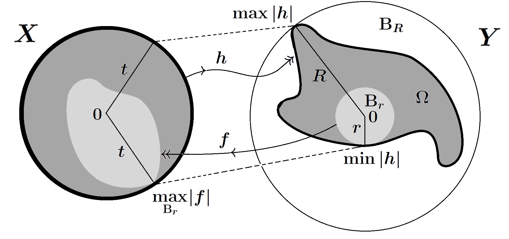
Figure 1. The ratio $\,\frac{R}{r}\leqslant\mathscr{K}\,$

Now the inverse map $\,f:\mathbb{Y}\xrightarrow[]{{}_{\!\!\textnormal{onto\,\,}\!\!}}\mathbb{X}\,$ takes $\,\Omega\,$ onto $\,\mathbb{B}(x_{\circ},t)\,$. In particular, it takes the common point of $\,\partial\mathbf{B}_{r}\,$ and $\,\partial\Omega\,$ into a point of $\,\partial\mathbb{B}(x_{\circ},t)\,$. This means that

$$t=\max_{|y|=r}|f(y)|\stackrel{{\scriptstyle\textnormal{def}}}{{=\!\!=}}\omega_{f}(r)$$

The proof is completed by invoking the quasi-inverse condition at (3.14),

$$R=\omega_{h}(t)=\omega_{h}(\omega_{f}(r))\leqslant\mathscr{K}r$$

∎

3.0.1. Doubling Property

It is worth discussing another special property of quasiconformal mappings in relation to their bi-modulus of continuity. To simplify matters we confine ourselves to quasiconformal mappings defined on the entire space, $\,h:\mathbb{R}^{n}\xrightarrow[]{{}_{\!\!\textnormal{onto\,\,}\!\!}}\mathbb{R}^{n}\,$ and its inverse $\,f:\mathbb{R}^{n}\xrightarrow[]{{}_{\!\!\textnormal{onto\,\,}\!\!}}\mathbb{R}^{n}\,$. It turns out that at every point $\,x_{\circ}\in\mathbb{R}^{n}\,$ the optimal modulus of continuity $\,\phi(t)\stackrel{{\scriptstyle\textnormal{def}}}{{=\!\!=}}\omega_{h}(x_{\circ};t)\,$, as well as its inverse function $\,\phi^{-1}:[0,\infty)\xrightarrow[]{{}_{\!\!\textnormal{onto\,\,}\!\!}}[0,\infty)\,$ have a doubling property. Observe that $\,\phi^{-1}\,$ is not exactly the optimal modulus of continuity of the inverse map $\,f=h^{-1}\,$, the latter is only quasi-inverse to $\,\phi^{-1}\,$. It should be emphasized at this point that doubling property of the modulus of continuity is rather rare, see our representative examples in Section 6.

Proposition 3.8.

Consider all $\,K\,$-quasiconformal mappings $\,h:\mathbb{R}^{n}\xrightarrow[]{{}_{\!\!\textnormal{onto\,\,}\!\!}}\mathbb{R}^{n}\,$. To every $\,\lambda\geqslant 1\,$ there corresponds a constant $\,\mathscr{K}_{\lambda}\,$ (actually the one specified in (3.11) ), and there is a constant $\,C_{\lambda}=C_{\lambda}(n,K)\,$ (independent of $\,h\,$) such that at every point $\,x_{\circ}\in\mathbb{R}^{n}\,$ we have

(3.18) $$\omega_{h}(x_{\circ};\lambda\,t)\leqslant\mathscr{K}_{\lambda}\,\,\omega_{h}(x_{\circ};t)\;$$

and

(3.19) $$\omega_{h}^{-1}(x_{\circ};\lambda\,s)\leqslant C_{\lambda}\,\,\omega_{h}^{-1}(x_{\circ};s)$$

for all $\,0\leqslant t<\infty\,$ and $\,0\leqslant s<\infty\,$.

Proof.

We may again assume that $\,x_{\circ}=0\,$ and $\,h(x_{\circ})=0\,$. This simplifies the notation $\,\omega_{h}(x_{\circ};t)\stackrel{{\scriptstyle\textnormal{def}}}{{=\!\!=}}\omega_{h}(t)\,$. The proof of the first inequality is immediate from the three points ratio condition in Proposition 3.5 , which gives us exactly the constant $\,\mathscr{K}_{\lambda}\,$ from this condition. Indeed, we have

• $\,\omega_{h}(\lambda\,t)=|h(x_{1})|\,$,  for some $\,x_{1}\in\mathbb{R}^{n}\,$ with $\,|x_{1}|=\lambda\,t\,$

• $\,\omega_{h}(t)\;=\;|h(x_{2})|\,$,   for some $\,x_{2}\in\mathbb{R}^{n}\,$ with $\,|x_{2}|=\,t\,$

• Hence, $\,\frac{|x_{1}|}{|x_{2}|}\;\leqslant\,\lambda\,.$

• Consequently $\,\frac{|h(x_{1})|}{|h(x_{2})|}\;\leqslant\,\mathscr{K}_{\lambda}\,$, which is the desired estimate.

∎

Clearly, for every $\,y_{\circ}\in\mathbb{R}^{n}\,$ we also have

(3.20) $$\omega_{f}(y_{\circ};\lambda\,s)\leqslant\mathscr{K}_{\lambda}\,\,\omega_{f}(y_{\circ};s)\;\;\;\;\textnormal{for all }\;\;0\leqslant s<\infty\,,$$

simply by interchanging the roles of $\,h\,$ and $\,f\,$.

We precede the proof of the doubling condition for $\,\omega_{h}^{-1}\,$, with a quick lemma.

3.0.2. A quick lemma on doubling condition

Consider an arbitrary continuously increasing function $\,\phi:[0,\infty)\xrightarrow[]{{}_{\!\!\textnormal{onto\,\,}\!\!}}[0,\infty)\,$ (in our application, $\,\phi(t)=\omega_{h}(t)\,$). It is commonly said that $\,\phi\,$ satisfies doubling condition if there is a constant $\,C_{\phi}\geqslant 1\,$ such that $\,\phi(2t)\leqslant C_{\phi}\,\phi(t)\,$ for all $\,t\geqslant 0\,$. However, it is convenient to work with so-called generalized doubling condition, which reads as:

(3.21) $$\phi(\lambda\,t)\leqslant C_{\phi}(\lambda)\,\phi(t)\;,\;\;\textnormal{for all}\;t\geqslant 0$$

where the $\,\lambda\,$- constant  $\,C_{\phi}(\lambda)\geqslant 1\,$ is obtained by iterating the inequality $\,\phi(2\,t)\leqslant C_{\phi}\,\phi(t)\,$.
Associated with $\,\phi\,$ is its quasi-inverse function. This term pertains to any continuous and strictly increasing function $\,\psi:[0,\infty)\xrightarrow[]{{}_{\!\!\textnormal{onto\,\,}\!\!}}[0,\infty)\,$ such that

(3.22) $$m\,t\leqslant\psi(\phi(t))\;\leqslant Mt\;,\;\;\textnormal{for all}\;t\geqslant 0$$

where $\,0<m\leqslant 1\leqslant M<\infty\,$ are constants. In general, $\,\psi\,$ does not satisfy doubling condition, but its inverse $\,\psi^{-1}:[0,\infty)\xrightarrow[]{{}_{\!\!\textnormal{onto\,\,}\!\!}}[0,\infty)\,$ does.

Lemma 3.9.

To every factor $\,\lambda\geqslant 1\,$ there corresponds a generalized doubling constant for $\,\psi^{-1}\,$. For all $\,t\geqslant 0\,$ we have

(3.23) $$\psi^{-1}(\lambda\,t)\leqslant C_{\psi^{-1}}(\lambda)\,\,\psi^{-1}(t)\;.\;\;\;\textnormal{Explicitly}\,\;C_{\psi^{-1}}(\lambda)\stackrel{{\scriptstyle\textnormal{def}}}{{=\!\!=}}C_{\phi}\left(M\lambda/m\right)\,.$$

Proof.

Choose and fix $\,\lambda\geqslant 1\,$. Inequality (3.22) is equivalent to:

(3.24) $$\psi^{-1}(m\,t)\leqslant\phi(t)\;\leqslant\psi^{-1}(Mt)\,,\;\;\textnormal{for all}\;t\geqslant 0\,.$$

Upon substitution $\,t\rightsquigarrow\frac{\lambda t}{m}\,$ in the left hand side, we obtain

$\psi^{-1}(\lambda\,t)\leqslant\phi(\frac{\lambda\,t}{m})\;=\;\phi(\frac{M\lambda}{m}\,\cdot\,\frac{t}{M})\leqslant\,C_{\phi}(\frac{M\lambda}{m})\,\cdot\,\phi(\frac{t}{M})$

The proof of the lemma is completed by invoking the right hand side of inequality (3.24) which, upon substitution $\,t\rightsquigarrow\frac{t}{M}\,$, gives us the desired estimate $\,\phi(\frac{t}{M})\leqslant\psi^{-1}(t)\,$. ∎

We summarize this section with the following theorem, which is an expanded version of Theorem 1.1:

Theorem 3.10.

Let $\,h:\mathbb{R}^{n}\xrightarrow[]{{}_{\!\!\textnormal{onto\,\,}\!\!}}\mathbb{R}^{n}\,$ be a $\,K\,$-quasiconformal mapping and $\,f:\mathbb{R}^{n}\xrightarrow[]{{}_{\!\!\textnormal{onto\,\,}\!\!}}\mathbb{R}^{n}\,$ its inverse. Choose and fix an arbitrary point $\,x_{\circ}\in\mathbb{R}^{n}\,$ an its image point $\,y_{\circ}=h(x_{\circ})\,$. Denote by $\,\phi(t)=\omega_{h}(x_{\circ};t)\,$ the optimal modulus of continuity of $\,h\,$ at $\,x_{\circ}\,$ and by $\,\psi(s)=\omega_{f}(y_{\circ};s)\,$ the optimal modulus of continuity of $\,f\,$ at $\,y_{\circ}\,$. Then the following statements hold true.

• The functions $\,\phi\,$ and $\,\psi\,$ are quasi-inverse to each other. Precisely, there is a constant $\,\mathscr{K}=\mathscr{K}(n,K)\,$ such that

  (3.25) $$\mathscr{K}^{-1}\,t\,\leqslant\psi(\phi(t))\;\leqslant\mathscr{K}\,t\;\;\textnormal{ and }\;\;\mathscr{K}^{-1}\,s\,\leqslant\phi(\psi(s))\;\leqslant\mathscr{K}\,s$$

  for all $\,t,s\in[0,\infty)\,$.

• Both $\,\phi\,$ and $\,\psi\,$ satisfy the general doubling condition; that is, for every $\,\lambda\geqslant 1\,$ there is a constant $\,\mathscr{K}_{\lambda}\,$ such that

  (3.26) $$\phi(\lambda\,t)\;\leqslant\mathscr{K}_{\lambda}\,\,\phi(t)\;\;\textnormal{ and }\;\;\psi(\lambda\,s)\,\leqslant\mathscr{K}_{\lambda}\,\,\psi(s)$$

  for all $\,t,s\in[0,\infty)\,$.

• As a consequence of Conditions $\,(Q1)\,$ and $\,(Q2)\,$, the inverse functions $\,\psi^{-1}\,$ and $\,\phi^{-1}\,$ also satisfy a general doubling conditions; namely,

  (3.27) $$\phi^{-1}(\lambda\,s)\;\leqslant C_{\lambda}\,\,\phi^{-1}(s)\;\;\textnormal{ and }\;\;\psi^{-1}(\lambda\,t)\,\leqslant C_{\lambda}\,\,\psi^{-1}(s)$$

  for all $\,t,s\in[0,\infty)\,$, where the constant $\,C_{\lambda}=\mathscr{K}_{\lambda}(\lambda\,\mathscr{K}^{2})\,$.

Let us now proceed to more general mappings of bi-conformal energy.

4. A handy metric in $\,\mathbb{R}^{n}\,\simeq\,\mathbb{R}^{n-1}\times\mathbb{R}$

It will be convenient to consider the space $\,\mathbb{R}^{n}\,$ as Cartesian product $\,\mathbb{R}^{n-1}\times\mathbb{R}\,$, with the purpose of using cylindrical coordinates. Accordingly,

$$\mathbb{R}^{n}=\mathbb{R}^{n-1}\times\mathbb{R}\,=\,\big{\{}X=(x,t);\;x=(x_{1},...,x_{n-1})\in\mathbb{R}^{n-1}\;\,\textnormal{and}\,\;t\in\mathbb{R}\,\big{\}}$$

Hereafter, we change the notation of the variables; the lowercase letter $\,x\,$ designates a point $\,(x_{1},...x_{n-1})\in\mathbb{R}^{n-1}\,$ while the uppercase letter $\,X=(x,t)\,$ is reserved for points in $\,\mathbb{R}^{n}\,$. The Euclidean norm of $\,x\in\mathbb{R}^{n-1}\,$ is denoted by $\,|x|\stackrel{{\scriptstyle\textnormal{def}}}{{=\!\!=}}\sqrt{x_{1}^{2}+\,\cdots\,+x_{n-1}^{2}}\,$. The space $\,\mathbb{R}^{n-1}\times\mathbb{R}\,$ is furnished with the norm

$$\,|\!|\,X\,|\!|\,\stackrel{{\scriptstyle\textnormal{def}}}{{=\!\!=}}|x|+|t|\,,\;\;\textnormal{for}\;\;X=(x,t)=(x_{1},...,x_{n-1},t)\in\mathbb{R}^{n-1}\times\mathbb{R}$$

In this metric the closed unit ball in $\,\mathbb{R}^{n-1}\times\mathbb{R}\,$ becomes the Euclidean double cone

$$\mathcal{C}\,=\,\{(x,t)\in\mathbb{R}^{n}\;;\;|x|+|t|\leqslant 1\;\;\}\;=\;\mathcal{C}_{+}\cup\mathcal{C}_{-}\;\;$$

where we split $\,\mathcal{C}\,$ into the upper and lower cones:

$$\mathcal{C}_{+}\,=\,\{(x,t);\;|x|+t\leqslant 1\;,\;t\geqslant 0\;\}\;\;,\;\;\mathcal{C}_{-}\,=\,\{(x,t);\;|x|-t\leqslant 1\;,\;t\leqslant 0\;\}$$

5. The idea of the construction of $\,H:\mathcal{C}\xrightarrow[]{{}_{\!\!\textnormal{onto\,\,}\!\!}}\mathcal{C}\,$

Our construction of a bi-conformal energy map $\,H:\mathcal{C}\xrightarrow[]{{}_{\!\!\textnormal{onto\,\,}\!\!}}\mathcal{C}\,$, whose optimal modulus of continuity at the origin coincides with that of the inverse map, will be carried out in two steps. First we construct a homeomorphism $\,H:\mathcal{C}_{+}\xrightarrow[]{{}_{\!\!\textnormal{onto\,\,}\!\!}}\mathcal{C}_{+}\,$ of finite conformal-energy which equals the identity on $\,\partial\,\mathcal{C}_{+}\,$. Its inverse map $\,F\stackrel{{\scriptstyle\textnormal{def}}}{{=\!\!=}}H^{-1}\,:\,\mathcal{C}_{+}\xrightarrow[]{{}_{\!\!\textnormal{onto\,\,}\!\!}}\mathcal{C}_{+}\,$ will also have finite conformal-energy. The substance of the matter is that their optimal moduli of continuity ($\,\omega_{{}_{H}}\,$ and $\,\omega_{{}_{F}}\,$, respectively) are inverse to each other; thus generally not equal. In fact $\omega_{H}$ will be stronger that $\omega_{F}$. In the second step we adopt the modulus of continuity of $\,F:\mathcal{C}_{+}\xrightarrow[]{{}_{\!\!\textnormal{onto\,\,}\!\!}}\mathcal{C}_{+}\,$ to an extension of $\,H\,$ to $\mathcal{C}_{-}$, simply by reflecting $\,F\,$ twice about $\,\mathbb{R}^{n-1}\,$. Let the reflection $\,\mathfrak{r}:\mathbb{R}^{n}\xrightarrow[]{{}_{\!\!\textnormal{onto\,\,}\!\!}}\mathbb{R}^{n}\,$ be defined by $\,\mathfrak{r}(x,t)=(x,-t)\,$. This gives rise to a map $\,\mathfrak{r}\circ F\circ\mathfrak{r}\,:\mathcal{C}_{-}\xrightarrow[]{{}_{\!\!\textnormal{onto\,\,}\!\!}}\mathcal{C}_{-}$, which we glue to $\,H:\mathcal{C}_{+}\xrightarrow[]{{}_{\!\!\textnormal{onto\,\,}\!\!}}\mathcal{C}_{+}\,$ along the common base $\,\partial\mathcal{C}_{+}\cap\partial\mathcal{C}_{-}\subset\mathbb{R}^{n-1}\,$. Precisely, the desired homeomorphism $\,H:\mathcal{C}\xrightarrow[]{{}_{\!\!\textnormal{onto\,\,}\!\!}}\mathcal{C}\,$, still denoted by $\,H\,$, will be defined by the rule

(5.1) $$H\stackrel{{\scriptstyle\textnormal{def}}}{{=\!\!=}}\left\{\begin{array}[]{l}H:\mathcal{C}_{+}\xrightarrow[]{{}_{\!\!\textnormal{onto\,\,}\!\!}}\mathcal{C}_{+}\\ \mathfrak{r}\circ F\circ\mathfrak{r}\,:\mathcal{C}_{-}\xrightarrow[]{{}_{\!\!\textnormal{onto\,\,}\!\!}}\mathcal{C}_{-}\end{array}\right.$$

Its inverse, also denoted by $\,F:\mathcal{C}\xrightarrow[]{{}_{\!\!\textnormal{onto\,\,}\!\!}}\mathcal{C}\,$, is defined analogously by interchanging the roles of $\,F\,$ and $\,H\,$.

(5.2) $$F\stackrel{{\scriptstyle\textnormal{def}}}{{=\!\!=}}\left\{\begin{array}[]{l}F:\mathcal{C}_{+}\xrightarrow[]{{}_{\!\!\textnormal{onto\,\,}\!\!}}\mathcal{C}_{+}\\ \mathfrak{r}\circ H\circ\mathfrak{r}\,:\mathcal{C}_{-}\xrightarrow[]{{}_{\!\!\textnormal{onto\,\,}\!\!}}\mathcal{C}_{-}\end{array}\right.$$

As a result, the optimal modulus of continuity of $\,H\,$ will be attained in the upper cone $\,\mathcal{C}_{+}\,$, whereas the optimal modulus of continuity of $\,F\,$ will be attained in the lower cone $\,\mathcal{C}_{-}\,$. Clearly, they are the same for the double cone $\mathcal{C}=\mathcal{C}_{+}\cup\mathcal{C}_{-}$, and this is the essence of our construction.
Explicit formula for $\,H\,$ can easily be stated, see Definition 7.1 in Section 7. Since $\,H:\mathcal{C}\xrightarrow[]{{}_{\!\!\textnormal{onto\,\,}\!\!}}\mathcal{C}\,$ and its inverse $\,F\stackrel{{\scriptstyle\textnormal{def}}}{{=\!\!=}}H^{-1}:\mathcal{C}\xrightarrow[]{{}_{\!\!\textnormal{onto\,\,}\!\!}}\mathcal{C}\,$ are both equal to the identity on $\,\partial\mathcal{C}\,$ we can extend them to $\,\mathbb{R}^{n}\,$ as the identity outside $\,\mathcal{C}\,$. Whenever it is convenient, we shall speak of $\,H:\mathbb{R}^{n}\xrightarrow[]{{}_{\!\!\textnormal{onto\,\,}\!\!}}\mathbb{R}^{n}\,$ and its inverse $\,F:\mathbb{R}^{n}\xrightarrow[]{{}_{\!\!\textnormal{onto\,\,}\!\!}}\mathbb{R}^{n}\,$ as homeomorphisms of the entire space $\,\mathbb{R}^{n}\,$ onto itself.

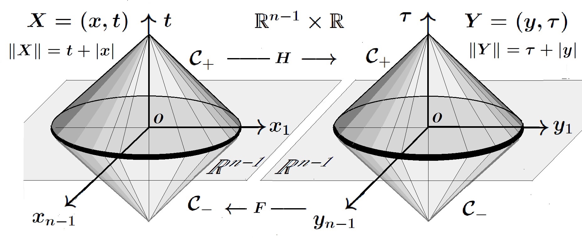
Figure 2. A mapping $\,H:\mathcal{C}\xrightarrow[]{{}_{\!\!\textnormal{onto\,\,}\!\!}}\mathcal{C}\,$ and its inverse $\,F:\mathcal{C}\xrightarrow[]{{}_{\!\!\textnormal{onto\,\,}\!\!}}\mathcal{C}\,$, will have the same optimal modulus of continuity at the center of $\mathcal{C}$.

6. Preconditions on the modulus of continuity
and the representative examples

Let us introduce a fairly general class of moduli of continuity to be considered. These classes are intended to unify the proofs. It will also give us an aesthetic appearance of the inequalities. On that account, our moduli of continuity, will be made of functions $\,\phi:[0,1]\xrightarrow[]{{}_{\!\!\textnormal{onto\,\,}\!\!}}[0,1]\,$ in $\,\mathscr{C}[0,1]\cap\mathscr{C}^{1}(0,1]\,$ such that:

• $\,\phi(0)=0\,,\;\phi(1)=1\,$    ( can be extended by $\phi(s)=s\,$  for  $\,s\geqslant 1\,$)

• (6.1) $$\phi^{\prime}(s)\leqslant\frac{\phi(s)}{s}\leqslant M[\phi^{\prime}(s)]^{2}\;,\;\textnormal{for some contant}\;1\leqslant M\,<\infty\,$$

• Finite Energy Condition :

  (6.2) $$E[\phi]\stackrel{{\scriptstyle\textnormal{def}}}{{=\!\!=}}\int_{0}^{1}|\phi(s)|^{n}\,\frac{\textnormal{d}s}{s}\;<\infty\,.$$

As a consequence of Conditions $\,(\textbf{C}_{1})\,$ and $\,(\textbf{C}_{2})\,$ we have:

• (6.3) $$\lambda(s)\stackrel{{\scriptstyle\textnormal{def}}}{{=\!\!=}}\frac{\phi(s)}{s}\,\geqslant\phi^{\prime}(s)\geqslant\frac{1}{M}\,\,\;\;\textnormal{for all }\,\,\,0<s\leqslant 1\,$$

  In the forthcoming representative examples (except for $\,\phi(s)\equiv s)\,$ we have even stronger property; namely, $\,\lim_{s\rightarrow 0}\phi^{\prime}(s)=\infty\,$ .

• The function $\,\lambda(s)\,$ is non-increasing. This follows from

  (6.4) $$\lambda^{\prime}(s)=\frac{\phi^{\prime}(s)}{s}\;-\,\frac{\phi(s)}{s^{2}}\;\leqslant 0.$$

• Thus in fact,

  (6.5) $$\,\lambda(s)\;=\;\frac{\phi(s)}{s}\geqslant\;\frac{\phi(1)}{1}=1\,\;,\;\textnormal{for all}\;\,0<s\leqslant 1\,$$

6.1. Representative examples

• For $\,\;\;0<\varepsilon\leqslant 1\,$, we set

  $$\phi_{{}_{0}}(s)=s^{\,\varepsilon}\;.\;\;\;\;\textnormal{In the borderline case,}\;\;\,\phi(s)=s\,$$

• For $\,\frac{1}{n}<\alpha\leqslant 1\,$, we set

  $$\phi_{{}_{1}}(s)\,=\,\log^{-\alpha}\left(\frac{e}{s}\right)\;\;=\left(1+a_{1}\log\frac{1}{s}\right)^{-\alpha}$$

• For $\,\frac{1}{n}<\alpha\leqslant 1\,$, we set

  $$\phi_{{}_{2}}(s)=\left(1+a_{1}\log\frac{1}{s}\right)^{-\frac{1}{n}}\left(1+a_{2}\log\log\frac{e}{s}\right)^{-\alpha}$$

• For $\,\frac{1}{n}<\alpha\leqslant 1\,$, we set

  $$\phi_{{}_{3}}(s)=\left(1+a_{1}\log\frac{1}{s}\right)^{-\frac{1}{n}}\left(1+a_{2}\log\log\frac{e}{s}\right)^{-\frac{1}{n}}\left(1+a_{3}\log\log\log\frac{e^{e}}{s}\right)^{-\alpha}$$

Continuing in this fashion, we define a sequence of functions $\,\phi_{{}_{k}}\,,\;k=0,1,2,...\,$ in which the last product-term in the round parantheses involves $\,k\,$-times iterated logarithm and $\,(k-1)\,$-times iterated power of $\,e\,$. All the above functions can be extended by setting $\,\phi_{k}(s)\equiv s,$ for $\,s\geqslant 1\,$.

Remark 6.1.

The coefficients $\,a_{k}\,$ in the above formulas are adjusted to ensure the inequality $\,\phi^{\prime}(s)\leqslant\frac{\phi(s)}{s}\,$, which is required by Condition $(\textbf{C}_{2})\,$. This works well with $\,a_{k}\stackrel{{\scriptstyle\textnormal{def}}}{{=\!\!=}}(1-\frac{1}{n})^{k-1}\,$. Indeed, the reader may wish to verify that the expression $\,\frac{s\phi_{k}^{\prime}(s)}{\phi_{k}(s)}\,$ is increasing, thus assumes its maximum value at $\,s=1\,$. It is then readily seen that its maximum value is not exceeding $\,\frac{1}{n}\,(a_{1}+a_{2}+...+a_{k-2})\;+\;\alpha\,a_{k}\;=\;1-\big{(}1-\alpha\big{)}\left(1-\frac{1}{n}\right)^{k-1}\;\leqslant 1\,$.

7. The definition of $\,H:\mathcal{C}_{+}\xrightarrow[]{{}_{\!\!\textnormal{onto\,\,}\!\!}}\mathcal{C}_{+}\,$ 

First we set $\,H\,$ on the vertical axis of the upper cone by the rule.

$$H(\textbf{0},t)=(\textbf{0},\phi(t))\,.$$

Here and below $(\textbf{0},t)\stackrel{{\scriptstyle\textnormal{def}}}{{=\!\!=}}(0,...,0\,,\,t)\in\mathbb{R}^{n-1}\times\mathbb{R}$. We wish $\,H\,$ to be the identity map on the base of the cone, which consists of points $\,(x,0)\in\mathbb{R}^{n-1}\times\mathbb{R}\,$ with $\,|x|\leqslant 1\,$. The idea is to connect $\,(x,0)\,$ with the point $\,(\textbf{0},|x|\,)\,$ by a straight line segment and map it linearly onto the straightline segment with endpoints at $\,(x,0)\,$ and $\,(\textbf{0},\phi(|x|)\,)\,$. Explicitly,

Definition 7.1.

The map $\,H:\mathcal{C}_{+}\xrightarrow[]{{}_{\!\!\textnormal{onto\,\,}\!\!}}\mathcal{C}_{+}\subset\mathbb{R}^{n-1}\times\mathbb{R}\,\,$ is given by the formula

(7.1) $$H(x,t)\stackrel{{\scriptstyle\textnormal{def}}}{{=\!\!=}}(x,\,t\,\lambda(t+|x|)\,)\;,\,\textnormal{for}\;0\leqslant t\leqslant 1\;\;\textnormal{and}\;|x|+t\leqslant 1$$

where we recall that $\,\lambda(s)\stackrel{{\scriptstyle\textnormal{def}}}{{=\!\!=}}\frac{\phi(s)}{s}\,\;\textnormal{for}\;\;0<s\leqslant 1\,.$

Indeed, for $\,\alpha,\beta\geqslant 0\,$ with $\,\alpha+\beta=1\,$, we have $\,H\big{[}\alpha\,(x,0)\;+\;\beta\,(\textbf{0 },|x|)\,\big{]}=\alpha\,(x,0)\;+\;\beta\,(\textbf{0 },\phi(|x|)\,$, which means that $\,H\,$ is a linear transformation between the above-mentioned segments. A formula for the inverse map $\,F:\mathcal{C}_{+}\xrightarrow[]{{}_{\!\!\textnormal{onto\,\,}\!\!}}\mathcal{C}_{+}\,$ is not that explicit.

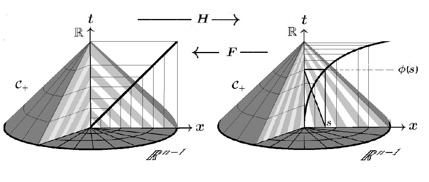
Figure 3. Diagonals of rectangles built on the curve $\,t=\phi(s)\,$. The map $\,F\,$ is linear on each such diagonal, as well as on their rotations.

8. The Jacobian matrix of $\,H\,$ and its inverse

A straightforward computation of the Jacobian matrix of $\,H\,$, at the point $\,X\stackrel{{\scriptstyle\textnormal{def}}}{{=\!\!=}}(x,t)=(x_{1},...,x_{n-1},t)\in\mathbb{R}^{n-1}\times\mathbb{R}\,$ shows that

(8.1) $$DH(x,\;t)=\left(\begin{array}[]{cccccc}1&0&0\ldots&0&0\\ $\;$\\ 0&1&0\ldots&0&0\\ \vdots&\vdots&\vdots\;\;\;\;\vdots&\vdots&\vdots\\ 0&0&0\ldots&1&0\\ $\;$\\ \mathfrak{D}_{1}&\mathfrak{D}_{2}&\mathfrak{D}_{3}\ldots&\mathfrak{D}_{n-1}&\mathfrak{D}\\ \end{array}\right)$$

where $\,\mathfrak{D}_{i}=\big{[}\,t\,\lambda^{\prime}(t+|x|)\,\big{]}\,\frac{x_{i}}{|x|}\,$  and $\,\mathfrak{D}=\lambda(t+|x|)\;+\;t\,\lambda^{\prime}(t+|x|)\,$ is the Jacobian determinant, later also denoted by $\,\mathbf{J}_{H}(X)\,$ . Then the inverse matrix $\,(DH)^{-1}\,$ takes the form

(8.2) $$(DH)^{-1}=\frac{1}{\mathfrak{D}}\,\left(\begin{array}[]{cccccc}\mathfrak{D}&0&0\ldots&0&0\\ $\;$\\ 0&\mathfrak{D}&0\ldots&0&0\\ \vdots&\vdots&\vdots\;\;\;\;\vdots&\vdots&\vdots\\ 0&0&0\ldots&\mathfrak{D}&0\\ $\;$\\ -\mathfrak{D}_{1}&-\mathfrak{D}_{2}&-\mathfrak{D}_{3}\ldots&-\mathfrak{D}_{n-1}&1\\ \end{array}\right)$$

Square of the Hilbert Schmidt norm of a matrix is the sum of squares of its entries. Accordingly,

(8.3) $$|DH|^{2}\,=\,n-1+\big{[}\,t\,\lambda^{\prime}(t+|x|)\,\big{]}^{2}\,+\big{[}\,\lambda(t+|x|)\,+\,t\,\lambda^{\prime}(t+|x|)\,\big{]}^{2}$$

and

(8.4) $$|\,(DH)^{-1}|^{2}\; = \;\frac{1\;}{\,\big{[}\,\lambda(t+|x|)\,+\,t\,\lambda^{\prime}(t+|x|)\,\big{]}^{2}}\;+$$

$$\frac{\big{[}\,t\,\lambda^{\prime}(t+|x|)\,\big{]}^{2}\;}{\,\big{[}\,\lambda(t+|x|)\,+\,t\,\lambda^{\prime}(t+|x|)\,\big{]}^{2}}\;\;+\;\;n-1$$

9. The Jacobian determinant $\mathfrak{D}\;=\;\mathbf{J}_{H}(X)$

We have the following bounds of the Jacobian determinant, including a uniform lower bound for all $\;X=(x,t)\,\in\mathcal{C}_{+}\,$.

(9.1) $$\,\lambda(\,|\!|\,X\,|\!|\,)\geqslant\mathbf{J}_{H}(X)\;\geqslant\phi^{\prime}(\,|\!|\,X\,|\!|\,)\geqslant\frac{1}{M}$$

Proof.

Using the notation $\,\,|\!|\,X\,|\!|\,=s=t+|x|\leqslant 1\,$, we write

$$\mathfrak{D}\; = \frac{\textnormal{d}}{\textnormal{d}t}\Big{(}t\,\lambda(t+|x|)\Big{)}=\frac{\textnormal{d}}{\textnormal{d}t}\Big{(}t\;\frac{\phi(t+|x|)}{t+|x|}\Big{)}=$$

$$\frac{\phi(s)}{s}\;+t\left(\frac{\phi^{\prime}(s)}{s}\;-\frac{\phi(s)}{s^{2}}\right)=\frac{\phi(s)}{s}\left(1-\frac{t}{s}\right)\;+t\,\frac{\phi^{\prime}(s)}{s}$$

Now, since $\,\phi^{\prime}(s)\leqslant\frac{\phi(s)}{s}=\lambda(s)\,$ , it follows that $\,\mathfrak{D}\leqslant\lambda(s)\,$. On the other hand $\,\phi^{\prime}(s)\geqslant\frac{1}{M}\,$ and $\,\frac{\phi(s)}{s}\geqslant 1\geqslant\frac{1}{M}\,$, whence $\,\mathfrak{D}\geqslant\frac{1}{M}\,$. ∎

10. Conformal-energy of $\,H:\mathcal{C}_{+}\xrightarrow[]{{}_{\!\!\textnormal{onto\,\,}\!\!}}\mathcal{C}_{+}\,$ 

In the forthcoming computation the ”implied constants” depend only on the dimension $\,n\geqslant 2\,$.

Lemma 10.1.

We have

(10.1) $$\int_{\mathcal{C}_{+}}|DH(x,t)|^{n}\,\,\textnormal{d}x\,\textnormal{d}t\;\preccurlyeq\;E[\phi]$$

Proof.

Formula (8.3) yields the inequality:

(10.2) $$\int_{\mathcal{C}_{+}}|DH(x,t)|^{n}\,\,\textnormal{d}x\,\textnormal{d}t\, \preccurlyeq \,1+\int_{t+|x|\,\leqslant 1}|\,\lambda(t+|x|)\,|^{n}\,\,\textnormal{d}x\,\textnormal{d}t$$

$$+\int_{t+|x|\,\leqslant 1}t^{n}|\,\lambda^{\prime}(t+|x|)\,|^{n}\,\,\textnormal{d}x\,\textnormal{d}t$$

Obviously, for the constant term we have $1\preccurlyeq\;E[\phi]\,$. For the first integral in the right hand side we make the substitution $\,t=s-|x|\,$ and use Fubini’s formula to obtain

$$\int_{t+|x|}\,|\lambda(t+|x|)\,|^{n}\,\textnormal{d}x\,\textnormal{d}t=\int_{|x|\leqslant s\leqslant 1}|\,\lambda(s)\,|^{n}\,\,\textnormal{d}x\,\textnormal{d}s\,=\,$$

$$=\int_{0}^{1}|\lambda(s)|^{n}\left(\int_{|x|\leqslant s}\textnormal{d}x\right)\textnormal{d}s=\frac{\omega_{n-2}}{n-1}\int_{0}^{1}s^{n-1}|\lambda(s)|^{n}\textnormal{d}s\,=\,\;$$

$$=\frac{\omega_{n-2}}{n-1}\int_{0}^{1}|\phi(s)|^{n}\;\frac{\textnormal{d}s}{s}\,\;\preccurlyeq\,\;E[\phi]\;$$

For the second integral in (10.2), we make the same substitution $\,t=s-|x|\,$ and proceed as follows

$$\int_{t+|x|\leqslant 1}t^{n}|\,\lambda^{\prime}(t+|x|)\,|^{n}\,\textnormal{d}x\,\textnormal{d}t=\int_{|x|\leqslant s\leqslant 1}\left(s-|x|\right)^{n}|\,\lambda^{\prime}(s)\,|^{n}\,\,\textnormal{d}x\,\textnormal{d}s$$

$$=\int_{0}^{1}|\lambda^{\prime}(s)|^{n}\left(\int_{|x|\leqslant s}\left(s-|x|\right)^{n}\textnormal{d}x\right)\textnormal{d}s$$

$$=\,c_{n}\int_{0}^{1}s^{2n-1}|\lambda^{\prime}(s)|^{n}\textnormal{d}s\preccurlyeq\int_{0}^{1}|\phi(s)|^{n}\,\frac{\textnormal{d}s}{s}\,=\,E[\phi]\,\;$$

Here, we used the inequality $\,|\lambda^{\prime}(s)\,|=\frac{\phi(s)}{s^{\,2}}-\frac{\phi^{\prime}(s)}{s}\leqslant\frac{\phi(s)}{s^{\,2}}\,$.
The proof is complete. ∎

11. Conformal-energy of the inverse map

This brings us back to the seminal work  [4]  on extremal mappings of finite distortion. Going into this in detail would take us too far afield, so we confine ourselves to a simplified variant.
Consider a homeomorphism $\,H:\mathbb{X}\xrightarrow[]{{}_{\!\!\textnormal{onto\,\,}\!\!}}\mathbb{Y}\,$ between bounded domains of Sobolev class $\,\mathscr{W}^{1,n}_{\textnormal{loc}}(\mathbb{X},\mathbb{Y})\,$ and assume (just to make it easier) that the Jacobian $\,\mathbf{J}_{H}\stackrel{{\scriptstyle\textnormal{def}}}{{=\!\!=}}\textnormal{det [DH]}\,$ is positive almost everywhere, as in (9.1).

Definition 11.1.

The differential expression

(11.1) $$\,\mathbf{K}_{H}(X)\stackrel{{\scriptstyle\textnormal{def}}}{{=\!\!=}}\big{|}\,[DH(X)]^{-1}\,\big{|}^{n}\;\mathbf{J}_{H}(X)\;=\;\frac{\big{|}\,D^{\sharp}H(X)\,\big{|}^{n}}{\;\left[\,\mathbf{J}_{H}(X)\,\right]^{n-1}}\,,$$

is called the inner distortion function of $\,H\,$. Here the symbol $\,D^{\sharp}H\,$ stands for the cofactor matrix of $\,DH\,$, defined by Cramer’s rule.

The following identity was first observed with a complete proof of it in [4] , see Theorem 9.1 therein.

Proposition 11.2.

Under the assumptions above, if $\,\mathbf{K}_{H}\in\mathscr{L}^{1}(\mathbb{X})\,$ then the inverse map $\,F:\mathbb{Y}\xrightarrow[]{{}_{\!\!\textnormal{onto\,\,}\!\!}}\mathbb{X}\,$ belongs to $\,\mathscr{W}^{1,n}(\mathbb{Y},\mathbb{X})\,$ and

(11.2) $$\int_{\mathbb{Y}}\big{|}\,DF(Y)\,\big{|}^{n}\,\textnormal{d}Y\;\;=\;\;\int_{\mathbb{X}}\mathbf{K}_{H}(X)\;\textnormal{d}X\,.$$

In our case, since $\,H\,$ is locally Lipschitz on $\,\mathcal{C}_{+}\,$, the derivation of this identity is straightforward. Simply, the differential matrix $\,DF(Y)\,$ at the point $\,Y=H(X)\,$ equals $\,[DH(X)]^{-1}\,$. We may change variables $\,Y=H(X)\,$ in the energy integral for $\,F\,$, to obtain

$$\int_{\mathcal{C}_{+}}\big{|}\,DF(Y)\big{|}^{n}\;\textnormal{d}Y\;=\int_{\mathcal{C}_{+}}\big{|}\,[DH(X)]^{-1}\,\big{|}^{n}\;\mathbf{J}_{H}(X)\,\textnormal{d}X\;\stackrel{{\scriptstyle\textnormal{def}}}{{=\!\!=}}\,\int_{\mathcal{C}_{+}}\mathbf{K}_{H}(X)\,\textnormal{d}X\;$$

Now, by (8.1) and (8.2), we have a point wise inequality $\,\mathbf{J}_{H}(X)\;\big{|}\,[DH(X)]^{-1}\,\big{|}\leqslant\sqrt{n-1}\,\big{|}\,DH(X)\,\big{|}\,$, which yields:

(11.3) $$\mathbf{K}_{H}\leqslant\frac{(n-1)^{\frac{n}{2}}|\,DH\,|^{n}}{(\mathbf{J}_{H})^{2n-1}}\leqslant(n-1)^{\frac{n}{2}}M^{2n-1}|\,DH\,|^{n}\,\in\mathscr{L}^{1}(\mathcal{C}_{+})$$

because $\,\mathbf{J}_{H}(X)\geqslant\frac{1}{M}\,$, by  (9.1).

12. Modulus of continuity of $\,H:\mathcal{C}_{+}\xrightarrow[]{{}_{\!\!\textnormal{onto\,\,}\!\!}}\mathcal{C}_{+}\,$

We start with the straightforward estimates of the modulus of continuity at $\,({\bf 0},0)\in\mathbb{R}^{n-1}\times\mathbb{R}\,$. In consequence of $\,\lambda(\,|\!|\,X\,|\!|\,)\geqslant 1\,$, we have :

$$\,|\!|\,X\,|\!|\,=|x|+t\,\,\leqslant|x|+t\,\lambda(t+|x|)\leqslant\,|x|\,\lambda(\,|\!|\,X\,|\!|\,)+t\,\lambda(\,|\!|\,X\,|\!|\,)\;=\,\phi(\,|\!|\,X\,|\!|\,)$$

Here the middle term $\,|x|+t\lambda(t+|x|)=\,|\!|\,\,H(X)\,|\!|\,\,$. Therefore,

(12.1) $$\,|\!|\,X\,|\!|\,\leqslant\,|\!|\,H(X)\,|\!|\,\;\leqslant\phi(\,|\!|\,X\,|\!|\,)$$

Corollary 12.1.

The function $\,\phi\,$ is the optimal modulus of continuity of the map $\,H:\mathcal{C}_{+}\xrightarrow[]{{}_{\!\!\textnormal{onto\,\,}\!\!}}\mathcal{C}_{+}\,$ at $\,({\bf 0},0)\in\mathbb{R}^{n-1}\times\mathbb{R}_{+}\,$; that is,

(12.2) $$\sup_{\,|\!|\,X\,|\!|\,=s}\,|\!|\,H(X)\,|\!|\,=\phi(s)\,,\;\;\textnormal{whenever}\;\;X\in\mathcal{C}_{+}\,\;\;\textnormal{and}\;0\leqslant s\leqslant 1$$

Indeed, the supremum is attained at the point $\,X\,=({\bf 0},s)\,$ on the vertical axis of the cone $\,\mathcal{C}_{+}\,$, because $\,H({\bf 0},s)=({\bf 0},\phi(s)\,)\,$.

Remark 12.2.

It is perhaps worth remarking in advance that both inequalities at (12.1) remain valid in terms of the Euclidean norm of $\,\mathbb{R}^{n}\,$ as well, where $\,|X|=|(x,t)|=\sqrt{|x|^{2}+t^{2}}\leqslant\,|\!|\,X\,|\!|\,\,$. To this end, since $\,\lambda\,$ is decreasing to its minimum value $\,\lambda(1)=1\,$, for $\,X\in\mathcal{C}_{+}\,$ we can write

$$|X|^{2}\leqslant|x|^{2}+t^{2}\lambda^{2}(\,|\!|\,X\,|\!|\,)\;=|H(X)|^{2}\leqslant|x|^{2}\lambda^{2}(|X|)+t^{2}\lambda^{2}(|X|)=\phi^{2}(|X|),$$

Let us record this fact as:

(12.3) $$|X|\leqslant|H(X)|\;\leqslant\phi(|X|)$$

For the inverse map $\,F=F(Y)\,$, these inequalities take the form

(12.4) $$\psi(|Y|)\leqslant|F(Y)|\;\leqslant|Y|\,\leqslant\phi(|Y|)\;\;\textnormal{for all}\;Y\in\mathcal{C}_{+}\,\;\textnormal{because}\;s\leqslant\phi(s)$$

where $\,\psi\,;\,[0,1]\xrightarrow[]{{}_{\!\!\textnormal{onto\,\,}\!\!}}[0,1]\,$ denotes the inverse function of $\,\phi\,$. This, however, does not necessarily imply that $\,F\,$ is Lipschitz continuous, as shown by our representative examples.

We shall now prove that $\,H\,$ admits $\,\phi\,$ as global modulus of continuity; that is, everywhere in $\,\mathcal{C}_{+}\,$. Precisely, we have

Proposition 12.3.

For $\,X=(x,t)\in\mathcal{C}_{+}\,$ and $\,X^{\prime}=(x^{\prime},t^{\prime})\in\mathcal{C}_{+}\,$ it holds that

(12.5) $$\,|\!|\,H(X)-H(X^{\prime})\,|\!|\,\;\leqslant 4\,\phi(\,|\!|\,X-X^{\prime}\,|\!|\,)\;$$

Thus, according to (2.3),

$$\Omega_{H}(t)\leqslant 4\phi(t)\,.$$

.

Proof.

Recall that $\,\,|\!|\,X\,\,|\!|\,\stackrel{{\scriptstyle\textnormal{def}}}{{=\!\!=}}|x|+|t|\,$ and $\,H(x,t)\stackrel{{\scriptstyle\textnormal{def}}}{{=\!\!=}}(\,x,\,t\lambda(\,|\!|\,X\,|\!|\,)\,)\,$. Thus

(12.6) $$\,|\!|\,H(X)-H(X^{\prime})\,|\!|\,\;\leqslant|x-x^{\prime}|\;+\;\;|t\lambda(\,|\!|\,X\,|\!|\,)\;-\;t^{\prime}\lambda(\,|\!|\,X^{\prime}\,|\!|\,)\,|$$

The first term is easily estimated as $\,|x-x^{\prime}|\leqslant\phi(|x-x^{\prime}|)\leqslant\phi(\,|\!|\,X-X^{\prime}\,|\!|\,)\,$, because $\ s\leqslant\phi(s)\,$ and $\,\phi\,$ is increasing in $\,s\in[0,1]\,$. The second term needs more work. First observe that for $\;0<A\leqslant B\leqslant 1\,$ it holds:

(12.7) $$0<\lambda(A)-\lambda(B)\;\leqslant A^{-1}\phi(B-A)$$

Indeed,

$$\begin{split}\lambda(A)\;-\;\lambda(B)&=n\frac{\phi(A)-\phi(B)}{A}\;+\;\frac{B-A}{A}\,\lambda(B)\\ &\leqslant\frac{B-A}{A}\,\lambda(B-A)=A^{-1}\phi(B-A)\end{split}$$

In the above formula, the first term is negative because $\,\phi\,$ is increasing. In the second term we have used the inequality $\,\lambda(B)\leqslant\lambda(B-A)\,$, because $\,\lambda\,$ is nonincreasing.
In Inequality (12.5) we may (and do) assume that $\,\,|\!|\,X^{\prime}\,|\!|\,\leqslant\,|\!|\,X\,|\!|\,\,$, for otherwise we can interchange $\,X\,$ with $\,X^{\prime}\,$. This yields $\,\frac{1}{2}\,\,|\!|\,X-X^{\prime}\,|\!|\,\leqslant\,|\!|\,X\,|\!|\,\,$ and, consequently, $\,\lambda(\,|\!|\,X\,|\!|\,)\leqslant\lambda(\frac{1}{2}\,|\!|\,X-X^{\prime}\,|\!|\,)=\phi(\frac{1}{2}\,|\!|\,X-X^{\prime}\,|\!|\,)/\frac{1}{2}\,|\!|\,X-X^{\prime}\,|\!|\,\leqslant 2\,\phi(\,|\!|\,X-X^{\prime}\,|\!|\,)/\,|\!|\,X-X^{\prime}\,|\!|\,\,$ . Having this and (12.7) at hand, we conclude with the desired estimate

$$\begin{split}|\;t\lambda(\,|\!|\,X\,|\!|\,)\;-\;t^{\prime}\lambda(\,|\!|\,X^{\prime}\,|\!|\,)\,\,|&\leqslant|\,t-t^{\prime}|\;\lambda(\,|\!|\,X\,|\!|\,)+t^{\prime}\,|\,\lambda(\,|\!|\,X\,|\!|\,)\;-\;\lambda(\,|\!|\,X^{\prime}\,|\!|\,)\,|\\ &\leqslant\frac{2\,|\,t-t^{\prime}|}{\,|\!|\,X-X^{\prime}\,|\!|\,}\;\phi(\,|\!|\,X-X^{\prime}\,|\!|\,)\\ &\;\;\;+\frac{t^{\prime}}{\,|\!|\,X^{\prime}\,|\!|\,}\;\phi(\,|\!|\,X\,|\!|\,-\,|\!|\,X^{\prime}\,|\!|\,)\\ &\leqslant 2\,\phi(\,|\!|\,X-X^{\prime}\,|\!|\,)\;\;+\;\phi(\,|\!|\,X-X^{\prime}\,|\!|\,)\\ &=3\,\phi(\,|\!|\,X-X^{\prime}\,|\!|\,)\end{split}$$

∎

13. Modulus of continuity of $\,F:\mathcal{C}_{+}\xrightarrow[]{{}_{\!\!\textnormal{onto\,\,}\!\!}}\mathcal{C}_{+}\,$

All representative functions $\,\phi=\phi_{k}\,,k=0,1,\dots$ that are listed in $(\mathbf{E}_{0})\dots(\mathbf{E}_{k})\dots$ are concave ($\,\phi_{k}^{\prime\prime}\leqslant 0\,\,$) near the origin, but not necessarily in the entire interval $\,[0,1]\,$. Actually, upon minor modifications away from the origin all the above functions can be made concave in the entire interval $\,[0,1]\,$. But their aesthetic appearance will be lost. Thus, rather than modifying those examples, in the first step we restrict our attention to a neighborhood of the origin. Outside such a neighborhood the mapping $\,F:\mathcal{C}_{+}\xrightarrow[]{{}_{\!\!\textnormal{onto\,\,}\!\!}}\mathcal{C}_{+}\,$ is Lipschitz continuous. This will take care of the global estimate.
The additional condition imposed on $\,\phi\,$ reads as follows:

• There is an interval $\,(0,r]\subset(0,1]\,$ in which $\phi\,$ is $\,\mathcal{C}^{2}\,$-smooth and concave; that is,

  (13.1) $$\phi^{\prime\prime}(s)\;\leqslant\;0\;,\;\;\textnormal{for}\;\;0<s\leqslant r$$

We shall now prove that $\,F\,$ admits $\,\phi\,$ as global modulus of continuity in $\,\mathcal{C}_{+}\,$.

Proposition 13.1.

For arbitrary two points $\,Y=(y,\tau)\in\mathcal{C}_{+}\,$ and $\,Y^{\prime}=(y^{\prime},\tau^{\prime})\in\mathcal{C}_{+}\,$ it holds:

(13.2) $$\,|\!|\,F(Y)-F(Y^{\prime})\,|\!|\,\;\;\preccurlyeq\,\;\phi(\,|\!|\,Y-Y^{\prime}\,|\!|\,)\;$$

The implied constant depends on the conditions imposed through $(\mathbf{C}_{1})-(\mathbf{C}_{4})\,.$

Proof.

A seemingly routine proof below, actually took an effort to accomplish all details. Let us begin with the definition of the map $\,H:\mathcal{C}_{+}\xrightarrow[]{{}_{\!\!\textnormal{onto\,\,}\!\!}}\mathcal{C}_{+}\,$ and some new related notation. For $\,X=(x,t)\in\mathcal{C}_{+}\subset\mathbb{R}^{n-1}\times\mathbb{R}\,$, we recall that

$$\,|\!|\,X\,|\!|\,=|x|\,+\,t\,\;\textnormal{and}\;\;H(X)=\big{(}x,t\,\lambda(t+|x|)\big{)}\;\stackrel{{\scriptstyle\textnormal{def}}}{{=\!\!=}}\;\big{(}y,\tau\big{)}\,=\,Y\in\mathbb{R}^{n-1}\times\mathbb{R}$$

For the inverse map $\,F=H^{-1}\,$ we write

$$\,|\!|\,Y\,|\!|\,\,=|y|\,+\tau\,\;\textnormal{and}\;\;F(Y)=\big{(}y,T\big{)}\in\mathcal{C}_{+}\subset\mathbb{R}^{n-1}\times\mathbb{R}$$

where the vertical coordinate $\,T=T(\tau,|y|)\,$ is determined uniquely from the equation

(13.3) $$\,T\,\lambda(T+|y|)\,=\,\tau\,$$

In much the same way as in (9) we find that the function $\,T\rightsquigarrow T\,\lambda(T+|y|)\,$ is strictly increasing. We actually have

$$\frac{\textnormal{d}\,T\,\lambda(T+|y|)}{\textnormal{d}T}=\lambda(T+|y|)\;+\;T\lambda^{\prime}(T+|y|)\;\geqslant\frac{1}{M}$$

Even more can be said about the above expression. Indeed, denoting by $\,s\stackrel{{\scriptstyle\textnormal{def}}}{{=\!\!=}}T+|y|\leqslant 1\,$, we have the identity

$$\lambda(s)+T\lambda^{\prime}(s)\;=\;\frac{\phi(s)}{s}\;+\;T\cdot\left(\frac{\phi^{\prime}(s)}{s}\,-\,\frac{\phi(s)}{s^{2}}\,\right)=\;\left(1-\frac{T}{s}\right)\frac{\phi(s)}{s}\;+\;\frac{T}{s}\cdot\phi^{\prime}(s)$$

which, in view of Condition ($\mathbf{C}_{2}$)  at (6.1), also yields a useful upper bound,

(13.4) $$\frac{\phi(s)}{s}\;\geqslant\lambda(s)+T\lambda^{\prime}(s)\;\geqslant\phi^{\prime}(s)\geqslant\,\frac{1}{M}$$

The latter follows from the Condition ($\mathbf{C}_{2}$)  at (6.1)  as well.
Now, implicit differentiation in (13.3) with respect to $\,\tau\,$-variable gives

(13.5) $$0\leqslant\frac{\partial T(\tau,|y|)}{\partial\tau}\;=\;\frac{1}{\lambda(T+|y|)\;+\;T\lambda^{\prime}(T+|y|)}\;\leqslant M$$

On the other hand, differentiation with respect to the $\,|y|\,$-variable gives

(13.6) $$0\leqslant\frac{\partial T(\tau,|y|)}{\partial\,|y|}\,=\,\frac{-\,T\lambda^{\prime}(T+|y|)}{\lambda(T+|y|)\,+\,T\lambda^{\prime}(T+|y|)}\,=\,\frac{-T\lambda^{\prime}(s)}{\lambda(s)\,+\,T\lambda^{\prime}(s)}$$

It should be noted that $\,\lambda^{\prime}(s)\leqslant 0\,$ whenever $\,s\stackrel{{\scriptstyle\textnormal{def}}}{{=\!\!=}}T+|y|\leqslant 1\,$. Precisely,

(13.7) $$0\leqslant\,-\lambda^{\prime}(s)\;=\;-\,\frac{\phi^{\prime}(s)}{s}\;+\;\frac{\phi(s)}{s^{2}}\;\leqslant\frac{\phi(s)}{s^{2}}\,$$

From this and the lower bound in (13.4) we infer that

$$0\leqslant\frac{\partial T(\tau,|y|)}{\partial\,|y|}\;\leqslant\;\frac{T\phi(s)}{s^{2}\phi^{\prime}(s)}\;\leqslant\;\frac{\phi(s)}{s\,\phi^{\prime}(s)}\;\leqslant\,M\phi^{\prime}(s)\,=M\phi^{\prime}(T+|y|),$$

the latter being guaranteed by the right hand side of inequality (6.1).

It is at this point that we are going to use the additional assumption that $\,\phi\,$ is concave near the origin; namely, $\,\phi^{\prime}\,$ is non-increasing in $\,(0,r]\subset(0,1]\,$. Examine an arbitrary point $\,Y=(y,\tau)\in\mathcal{C}_{+}\,$ of lengths $\,\,|\!|\,Y\,|\!|\,\stackrel{{\scriptstyle\textnormal{def}}}{{=\!\!=}}\,\tau+|y|\leqslant\frac{r}{M}\,$ to show that $\,T+|y|\leqslant r\,$. Recall that $\,T\,$ is determined by the equation $\,T\lambda(T+|y|)=\tau\,$. Thus, we have $\,\frac{T}{M}\leqslant\phi^{\prime}(T+|y|)\,T\;\leqslant\frac{\phi(T+|y|)}{T+|y|}\,T\;=\;\tau\,$, by Condition (6.1). Hence $\,T+|y|\leqslant M\tau+|y|\leqslant M(\tau+|y|)\;\leqslant r\,$. Since $\,s=T+|y|\geqslant|y|\,$ and $\,\phi^{\prime}\,$ is non-increasing in $\,(0,r]\,$ , we infer that

(13.8) $$0\leqslant\frac{\partial T(\tau,|y|)}{\partial\,|y|}\;\leqslant M\phi^{\prime}(|y|)\,\,,\;\;\textnormal{whenever}\;\tau+|y|\,\stackrel{{\scriptstyle\textnormal{def}}}{{=\!\!=}}\,\,|\!|\,Y\,|\!|\,\leqslant\frac{r}{M}$$

We are now ready to formulate an estimate of the modulus of continuity of $\,F\,$ within the neighborhood of the origin that is determined by $\,\,|\!|\,Y\,|\!|\,\leqslant\frac{r}{M}\,$.

Proposition 13.2.

Let $\,Y=(y,\tau)\in\mathbb{R}^{n-1}\times\mathbb{R}\,$ and $\,Y^{\prime}=(y^{\prime},\tau^{\prime})\in\mathbb{R}^{n-1}\times\mathbb{R}\,$ be points in $\,\mathcal{C}_{+}\,$ such that $\,\,|\!|\,Y\,|\!|\,\leqslant\frac{r}{M}\,$ and $\,\,|\!|\,Y^{\prime}\,|\!|\,\leqslant\frac{r}{M}\,$. Then

(13.9) $$\,|\!|\,F(Y)\;-\;F(Y^{\prime})\,\,|\!|\,\;\leqslant\;3M\phi(\,|\!|\,Y-Y^{\prime}\,|\!|\,)$$

Proof.

With the notation for $\,F(Y)=(y\,,\,T(\tau,|y|))\,$ and $\,F(Y^{\prime})=(y^{\prime}\,,\,T(\tau^{\prime},|y^{\prime}|))\,$ we begin with the computation,

$$\,|\!|\,F(Y)-F(Y^{\prime})\,\,|\!|\,=|y-y^{\prime}|\;+\;|\,T(\tau,|y|)-T(\tau^{\prime},|y^{\prime}|)\,|\;\leqslant$$

$$|y-y^{\prime}|\;+\;|\,T(\tau,|y|)-T(\tau,|y^{\prime}|)\,|\;+\;|\,T(\tau,|y^{\prime}|)-T(\tau^{\prime},|y^{\prime}|)\,|\leqslant(\textnormal{in view of}\;(\ref{T/tau}))$$

$$\leqslant\,|y-y^{\prime}|\;+\;|\,T(\tau,|y|)-T(\tau,|y^{\prime}|)\,|\;+\;M\,|\tau-\tau^{\prime}|\;\leqslant$$

$$|\,T(\tau,|y|)-T(\tau,|y^{\prime}|)\,|\,+\,M\,\,|\!|\,Y-Y^{\prime}\,|\!|\,\leqslant|\,T(\tau,|y|)-T(\tau,|y^{\prime}|)\,|\,+\,M\,\phi(\,|\!|\,Y-Y^{\prime}\,|\!|\,)$$

The latter is obtained by the inequality $\,s\leqslant\phi(s)\,$, see (6.5). It remains to establish the following estimates, say when $\,0<|y^{\prime}|\leqslant|y|\leqslant r\,.$

(13.10) $$|\,T(\tau,|y|)-T(\tau,|y^{\prime}|)\,|\;\leqslant 2M\phi(|y-y^{\prime}|)\;\leqslant\,2M\,\phi(\,|\!|\,Y-Y^{\prime}\,|\!|\,)$$

To that end, we begin with the following expression:

$$T(\tau,|y|)-T(\tau,|y^{\prime}|)\;=\int_{0}^{1}\frac{\textnormal{d}}{\textnormal{d}\gamma}\;\Big{[}T(\tau,|\gamma\,y+(1-\gamma)y^{\prime}|)\Big{]}\;\textnormal{d}\gamma$$

$$=\int_{0}^{1}\;T_{\xi}(\tau,|\gamma\,y+(1-\gamma)y^{\prime}|)\,\left\langle\frac{\gamma\,y+(1-\gamma)y^{\prime}\,}{|\gamma\,y+(1-\gamma)y^{\prime}|}\;\Big{|}\;y-y^{\prime}\,\right\rangle\,\textnormal{d}\gamma$$

where $\,T_{\xi}(\tau,\xi)\,\stackrel{{\scriptstyle\textnormal{def}}}{{=\!\!=}}\frac{\partial T(\tau,\xi)}{\partial\,\xi}\,$ . In view of (13.8) , we obtain

(13.11) $$|\;T(\tau,|y|)-T(\tau,|y^{\prime}|)\;|\leqslant\,M|y-y^{\prime}|\,\int_{0}^{1}\;\phi^{\prime}(|\gamma\,y+(1-\gamma)y^{\prime}|)\;\textnormal{d}\gamma$$

It is important to notice that $\,|\gamma\,y+(1-\gamma)y^{\prime}|\leqslant r\,$ , which enables us to invoke Condition $\,(\textbf{C}_{4})\,$ at (13.1); that is, $\,\phi^{\prime}\,$ is non-increasing in the interval $\,(0,r]\,$. The following interesting lemma comes into play.

Lemma 13.3.

Let $\,\Phi:(0,r]\rightarrow(0,\infty)\,$ be continuous non-increasing and integrable,

$$\int_{0}^{r}\Phi(s)\,\textnormal{d}s\;<\;\infty\;.$$

Then for every vectors $\,\mathfrak{a},\mathfrak{b}\,$ in a normed space $\,(\mathfrak{N}\,;\,|\,.\,|)\,$, such that   $\,0<|\mathfrak{a}|\leqslant r\,$ and $\,0<|\mathfrak{b}|\leqslant r\,$, it holds:

(13.12) $$\int_{0}^{1}\Phi(|\gamma\mathfrak{a}\;+\;(1-\gamma)\,\mathfrak{b}\,|)\,\textnormal{d}\gamma\;\leqslant\;\frac{1}{|\mathfrak{a}|+|\mathfrak{b}|}\left(\int_{0}^{|\mathfrak{a}|}\Phi(s)\,\textnormal{d}s\;+\;\int_{0}^{|\mathfrak{b}|}\Phi(s)\,\textnormal{d}s\right)$$

Equality occurs if $\,\mathfrak{a}\,$ is a negative multiple of $\,\mathfrak{b}\,$.

Proof.

Since $\,\phi\,$ is non-increasing, by triangle inequality it follows that

$$\int_{0}^{1}\Phi(|\gamma\mathfrak{a}\;+\;(1-\gamma)\,\mathfrak{b}\,|)\,\textnormal{d}\gamma\;\leqslant\;\int_{0}^{1}\Phi\left(\big{|}\,(1-\gamma)\,|\mathfrak{b}|\,-\,\gamma|\mathfrak{a}|\;\big{|}\right)\,\textnormal{d}\gamma\;=$$

$$\int_{0}^{\frac{|\mathfrak{b}|}{|\mathfrak{a}|+|\mathfrak{b}}|}\Phi\big{(}\,(1-\gamma)\,|\mathfrak{b}|\,-\,\gamma|\mathfrak{a}|\;\big{)}\,\textnormal{d}\gamma\;+\;\int_{\frac{|\mathfrak{b}|}{|\mathfrak{a}|+|\mathfrak{b}}|}^{1}\Phi\big{(}\,\gamma|\mathfrak{a}|\,-\,(1-\gamma)\,|\mathfrak{b}|\,\big{)}\,\textnormal{d}\gamma$$

In the first integral we make a substitution $\,s=(1-\gamma)\,|\mathfrak{b}|\,-\,\gamma|\mathfrak{a}|\,$, which places $\,s\,$ in the interval $\,(0,|\mathfrak{b}|\,)\,$ and $\,|\textnormal{d}s|=(|\mathfrak{a}|+|\mathfrak{b}|)\,\textnormal{d}\lambda\,$. This gives us the second integral-term of the right hand side of (13.12), and similarly for the first integral-term. ∎

Since $\,\phi^{\prime}\,$ is non-increasing in the interval $\,(0,r]\,$ (by inequality (13.1) at Condition  ($\mathbf{C}_{4}$) ), we may apply Estimate (13.12)  to $\,\Phi=\phi^{\prime}\,$. Now, returning to (13.11), the inequality  (13.10)  is readily inferred as follows:

$$|\;T(\tau,|y|)-T(\tau,|y^{\prime}|)\;|\leqslant\,M|y-y^{\prime}|\,\frac{\phi(|y|)+\phi(|y^{\prime}|)}{|y|+|y^{\prime}|}=$$

$$\,=\;M\,\phi(|y-y^{\prime}|)\,\frac{|y-y^{\prime}|}{\phi(|y-y^{\prime}|)}\,\frac{\phi(|y|)+\phi(|y^{\prime}|)}{|y|+|y^{\prime}|}\;\leqslant$$

$$\,\leqslant M\,\phi(|y-y^{\prime}|)\,\frac{|y|+|y^{\prime}|}{\phi(|y|+|y^{\prime}|)}\,\frac{\phi(|y|)+\phi(|y^{\prime}|)}{|y|+|y^{\prime}|}\;\leqslant 2\,M\,\phi(|y-y^{\prime}|)\,,$$

because $\,\frac{s}{\phi(s)}=\frac{1}{\lambda(s)}\,$  is non-decreasing, see  (6.4) , and $\,\phi(s)\,$ is increasing. The proof of Proposition 13.2  is complete. ∎

Finally, the global estimate (13.2) in Proposition 13.1 follows from Proposition 13.2, whenever $\,\,|\!|\,Y\,|\!|\,\leqslant\frac{r}{M}\,$ and $\,\,|\!|\,Y^{\prime}\,|\!|\,\leqslant\frac{r}{M}\,$. Whereas its extension to all points $\,Y\,$ and $\,Y^{\prime}\,$ is fairly straightforward by invoking Lipschitz continuity of $\,F\,$ away from the origin. ∎

14. Conclusion

Choose an arbitrary modulus of continuity function $\,\phi:[0,\infty)\xrightarrow[]{{}_{\!\!\textnormal{onto\,\,}\!\!}}[0,\infty)\,$ that satisfies conditions $\,(\mathbf{C}_{1})\,(\mathbf{C}_{2})\,(\mathbf{C}_{3})\,$ and $\,(\mathbf{C}_{4})\,$. Then consider a bi-conformal energy map $\,H:\mathcal{C}_{+}\xrightarrow[]{{}_{\!\!\textnormal{onto\,\,}\!\!}}\mathcal{C}_{+}\,$ defined in  (7.1) together with its inverse map $\,F:\mathcal{C}_{+}\xrightarrow[]{{}_{\!\!\textnormal{onto\,\,}\!\!}}\mathcal{C}_{+}\,$. Extend $\,H\,$ and $\,F\,$ to the double cone $\,\mathcal{C}=\mathcal{C}_{+}\cup\mathcal{C}_{-}\,$ by the reflection rule at  (5.1). Afterwards extend $\,H\,$ and $\,F\,$ to the entire space $\,\mathbb{R}^{n}\,$ by setting $\,H=\textnormal{Id}:\mathbb{R}^{n}\setminus\mathcal{C}\xrightarrow[]{{}_{\!\!\textnormal{onto\,\,}\!\!}}\mathbb{R}^{n}\setminus\mathcal{C}\,$ and $\,F=\textnormal{Id}:\mathbb{R}^{n}\setminus\mathcal{C}\xrightarrow[]{{}_{\!\!\textnormal{onto\,\,}\!\!}}\mathbb{R}^{n}\setminus\mathcal{C}\,$. Then we obtain:

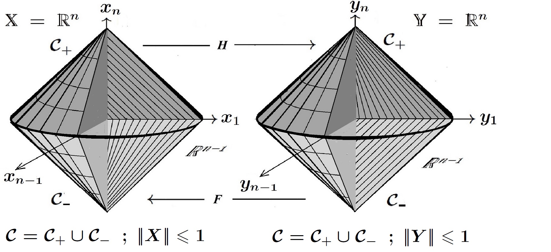
Figure 4. Bi-conformal energy mapping $\,H\,$ and its inverse $\,F\,$ exhibit the same optimal modulus of continuity at the origin of the double cone $\mathcal{C}$.

Theorem 14.1.

For every modulus of continuity function $\,\phi:[0,\infty)\xrightarrow[]{{}_{\!\!\textnormal{onto\,\,}\!\!}}[0,\infty)\,$ satisfying conditions $\,(\mathbf{C}_{1})\,(\mathbf{C}_{2})\,(\mathbf{C}_{3})\,$ and $\,(\mathbf{C}_{4})\,$, there exists a homeomorphism $\,H:\mathbb{R}^{n}\xrightarrow[]{{}_{\!\!\textnormal{onto\,\,}\!\!}}\mathbb{R}^{n}\,$ of Sobolev class $\,\mathscr{W}^{1,n}_{\textnormal{loc}}(\mathbb{R}^{n}\,,\,\mathbb{R}^{n})\,$, whose inverse $\,F=H^{-1}:\mathbb{R}^{n}\xrightarrow[]{{}_{\!\!\textnormal{onto\,\,}\!\!}}\mathbb{R}^{n}\,$ also lies in the Sobolev space $\,\mathscr{W}^{1,n}_{\textnormal{loc}}(\mathbb{R}^{n},\mathbb{R}^{n})\,.$ Moreover

• $\,H(0)=0\,,\;H(X)\equiv X\,,\;\textnormal{for}\;\,|\!|\,X\,|\!|\,\geqslant 1\,\,\textnormal{and for}\,X=(x_{1},...,x_{n-1},0)\,.$

• $\,H:\mathbb{R}^{n}\xrightarrow[]{{}_{\!\!\textnormal{onto\,\,}\!\!}}\mathbb{R}^{n}\,$ admits $\,\phi\,$ as its global modulus of continuity; that is,

  (14.1) $$\,|\!|\,\,H(X_{1})\,-\,H(X_{2})\,\,|\!|\,\;\,\preccurlyeq\,\;\phi(\,|\!|\,X_{1}-X_{2}\,|\!|\,)\;,\;\;\textnormal{for all}\;\;X_{1},X_{2}\in\mathbb{R}^{n}\,.$$

• The inverse map $\,F:\mathbb{R}^{n}\xrightarrow[]{{}_{\!\!\textnormal{onto\,\,}\!\!}}\mathbb{R}^{n}\,$ satisfies the same condition:

  (14.2) $$\,|\!|\,\,F(Y_{1})\,-\,F(Y_{2})\,\,|\!|\,\;\,\preccurlyeq\,\;\phi(\,|\!|\,Y_{1}-Y_{2}\,|\!|\,)\;,\;\;\textnormal{for all }Y_{1},Y_{2}\in\mathbb{R}^{n}\,.$$

• $H$ and $F$ share the same optimal moduli of continuity at the origin; namely

  (14.3) $$\omega_{{}_{H}}(0,r)=\max_{\,|\!|\,X\,|\!|\,=r}|H(X)|\;=\;\phi(r)\;=\;\max_{\,|\!|\,Y\,|\!|\,=r}|F(Y)|=\omega_{{}_{F}}(0,r)$$

  for all $0\leqslant r<\infty$.

References

- [1] S. S. Antman, Nonlinear problems of elasticity. Applied Mathematical Sciences, 107. Springer-Verlag, New York, 1995.
- [2] K. Astala, T. Iwaniec, and G. Martin, Deformations of annuli with smallest mean distortion, Arch. Ration. Mech. Anal. 195 (2010), no. 3, 899–921.
- [3] K. Astala, T. Iwaniec, and G. Martin, Elliptic partial differential equations and quasiconformal mappings in the plane, Princeton University Press, 2009.
- [4] K. Astala, T. Iwaniec, and G. Martin and J. Onninen, Extremal mappings of finite distortion, Proceedings of the London Math. Soc. (3) 91, no 3 (2005) 655–702.
- [5] J. M. Ball, Convexity conditions and existence theorems in nonlinear elasticity, Arch. Rational Mech. Anal. 63 (1976/77), no. 4, 337–403.
- [6] J. M. Ball, Discontinuous equilibrium solutions and cavitation in nonlinear elasticity, Philos. Trans. R. Soc. Lond. A 306 (1982) 557–611.
- [7] Bojarski, B., and Iwaniec, T. Analytical foundations of the theory of quasiconformal mappings in . Ann. Acad. Sci. Fenn. Ser. A I Math. 8 (1983), no. 2, 257–324.
- [8] P. Caraman, -Dimensional Quasiconformal Mappings, Editura Academiei Romãne, 1974.
- [9] D. Campbell and S. Hencl, A note on mappings of finite distortion: examples for the sharp modulus of continuity, Ann. Acad. Sci. Fenn. Math. 36 (2011), no. 2, 531–536.
- [10] P. G. Ciarlet, Mathematical elasticity Vol. I. Three-dimensional elasticity, Studies in Mathematics and its Applications, 20. North-Holland Publishing Co., Amsterdam, 1988.
- [11] A. Clop and D. Herron, Mappings with finite distortion in : modulus of continuity and compression of Hausdorff measure Israel J. Math. 200 (2014), no. 1, 225–250
- [12] J.-M. Coron, R.D. Gulliver, Minimizing p-harmonic maps into spheres, J. Reine Angew. Math. 401 (1989) 82–100.
- [13] F. W. Gehring, Rings and quasiconformal mappings in space, Trans. Amer. Math. Soc. 103, (1962) 353–393.
- [14] F. W. Gehring, Extension theorem for quasiconformal mappings in -space, J. Analyse Math. 19 (1967) 149–169.
- [15] F. W. Gehring, Topics in quasiconformal mappings, Proceedings of ICM, Vol 1, Berkeley (1986) 62–80; also, Quasiconformal Space Mappings- A collection of surveys 1960-1990, Springer-Verlag (1992), 20-38, Lecture Notes in Mathematics Vol. 1508.
- [16] F.W. Gehring and O. Martio, Quasiextremal Distance Domains and Extension of Quasiconformal Mappings, Journal D’Analyse Mathematique, vol 45 (1985) 181 –206.
- [17] V. M. Goldstein and S.K. Vodop’yanov, Quasiconformal mappings and spaces of functions with generelized first derivatives, Sb. Mat. Z., 17 (1076) 515–531.
- [18] R. Hardt, F.H. Lin, C.Y. Wang, The p-energy minimality of , Comm. Anal. Geom. 6 (1998) 141–152.
- [19] Heinonen, J., Kilpeläinen, T., and Martio, O. Nonlinear potential theory of degenerate elliptic equations. Oxford Mathematical Monographs, (1993).
- [20] S. Hencl and P. Koskela Lectures on mappings of finite distortion, Lecture Notes in Mathematics 2096, Springer, (2014).
- [21] D. A. Herron and P. Koskela, Mappings of finite distortion: gauge dimension of generalized quasicircles, Illinois J. Math. 47 (2003), no. 4, 1243–1259.
- [22] L. Hitruhin, Pointwise rotation for mappings with exponentially integrable distortion, Proc. Amer. Math. Soc. 144 (2016), no. 12, 5183–5195.
- [23] M.-C. Hong, On the minimality of the p-harmonic map , Calc. Var. Partial Differential Equations 13 (2001) 459–468.
- [24] T. Iwaniec , P. Koskela and J. Onninen, Mappings of finite distortion: monotonicity and continuity, Invent. Math. 144 (2001), no. 3, 507–531.
- [25] T. Iwaniec, L. V. Kovalev, and J. Onninen, The Nitsche conjecture, J. Amer. Math. Soc. 24 (2011), no. 2, 345–373.
- [26] T. Iwaniec, L. V. Kovalev, and J. Onninen, Doubly connected minimal surfaces and extremal harmonic mappings, J. Geom. Anal. 22 (2012), no. 3, 726–762.
- [27] T. Iwaniec and G. Martin, Geometric Function Theory and Non-linear Analysis, Oxford Mathematical Monographs, Oxford University Press, 2001.
- [28] T. Iwaniec and J. Onninen, Neohookean deformations of annuli, existence, uniqueness and radial symmetry, Math. Ann. 348 (2010), no. 1, 35–55.
- [29] T. Iwaniec and J. Onninen, Deformations of finite conformal energy: existence and removability of singularities, Proc. London Math. Soc., (3) 100 (2010) 1–23.
- [30] T. Iwaniec and J. Onninen, An invitation to n-harmonic hyperelasticity, Pure Appl. Math. Q. 7 (2011), no. 2, 319–343.
- [31] T. Iwaniec and J. Onninen, Deformations of finite conformal energy: boundary behavior and limit theorems, Trans. AMS 363 (2011) no 11, 5605–5648.
- [32] T. Iwaniec and J. Onninen, Hyperelastic deformations of smallest total energy, Arch. Ration. Mech. Anal. 194 (2009), no. 3, 927–986.
- [33] T. Iwaniec and J. Onninen, -Harmonic mappings between annuli, Memoirs of the Amer. Math. Soc. 218 (2012).
- [34] T. Iwaniec V. Šverák, On mappings with integrable dilatation, Proceedings of AMS vol. 118, no. 1 (1993) 181–188.
- [35] M. Jordens and G. J. Martin, Deformations with smallest weighted average distortion and Nitsche type phenomena, J. Lond. Math. Soc. (2) 85 (2012), no. 2, 282–300.
- [36] W. Jäger, H. Kaul, Rotationally symmetric harmonic maps from a ball into a sphere and the regularity problem for weak solutions of elliptic systems J. Reine Angew. Math. 343 (1983) 146–161.
- [37] J.A. Kelingos Characterization of quasiconformal mappings in terms of harmonic and hyperbolic measures, Ann. Acad. Sci. Fenn. Ser. A. I, No 368 (1965) 1–16.
- [38] P. Koskela and J. Onninen, Mappings of finite distortion: the sharp modulus of continuity, Trans. Amer. Math. Soc. 355 (2003), no. 5, 1905–1920.
- [39] A. Koski and J. Onninen, Radial symmetry of p-harmonic minimizers, Arch. Ration. Mech. Anal. 230 (2018), no. 1, 321–342.
- [40] H. Lebesgue, SSur les intégrales singuliéres, Ann. Fac. Sci. Univ. Toulouse. 3 (1909), pp. 25–117.
- [41] J. E. Marsden T. J. R. Hughes, Mathematical foundations of elasticity, Dover Publications, Inc., New York, 1994.
- [42] F. Meynard, Existence and nonexistence results on the radially symmetric cavitation problem, Quart. Appl. Math. 50 (1992) 201–226.
- [43] S. Müller, S. J. Spector, An existence theory for nonlinear elasticity that allows for cavitation, Arch. Rational Mech. Anal. 131 (1995) 1–66.
- [44] J. Onninen and V. Tengvall, Mappings of -integrable distortion: regularity of the inverse, Proc. Roy. Soc. Edinburgh Sect. A 146 (2016), no. 3, 647–663.
- [45] J. Onninen and X. Zhong, A note on mappings of finite distortion: the sharp modulus of continuity, Michigan Math. J. 53 (2005), no. 2, 329–335.
- [46] Reshetnyak, Yu. G. Space mappings with bounded distortion. Translations of Mathematical Monographs, 73. American Mathematical Society, Providence, RI, 1989.
- [47] Rickman, S. Quasiregular mappings. Springer-Verlag, Berlin, 1993.
- [48] J. Sivaloganathan, Uniqueness of regular and singular equilibria for spherically symmetric problems of nonlinear elasticity, Arch. Rational Mech. Anal. 96 (1986) 97–136.
- [49] J. Sivaloganathan and S. J. Spector, Necessary conditions for a minimum at a radial cavitating singularity in nonlinear elasticity, Ann. Inst. H. Poincaré Anal. Non Linéaire 25 (2008), no. 1, 201–213.
- [50] C.A. Stuart, Radially symmetric cavitation for hyperelastic materials, Anal. Non Liné aire 2 (1985) 33?66.
- [51] M. Vuorinen, Conformal geometry and quasiregular mappings, Lecture Notes in Mathematics, 1319. Springer-Verlag, Berlin, 1988.
- [52] J. Väisälä, Lectures on n-dimensional quasiconformal mappings, Lecture Notes in Mathematics, Vol. 229. Springer-Verlag, Berlin-New York, (1971).
- [53] J. Väisälä, On quasiconformal mappings in space, Ann. Acad. Sci. Fenn. Ser. AI 298 (1961) 1–36.