A unifying approach for doubly-robust $\ell_{1}$ regularized estimation of causal contrasts

Abstract

We consider inference about a scalar parameter under a non-parametric model based on a one-step estimator computed as a plug in estimator plus the empirical mean of an estimator of the parameter’s influence function. We focus on a class of parameters that have influence function which depends on two infinite dimensional nuisance functions and such that the bias of the one-step estimator of the parameter of interest is the expectation of the product of the estimation errors of the two nuisance functions. Our class includes many important treatment effect contrasts of interest in causal inference and econometrics, such as ATE, ATT, an integrated causal contrast with a continuous treatment, and the mean of an outcome missing not at random. We propose estimators of the target parameter that entertain approximately sparse regression models for the nuisance functions allowing for the number of potential confounders to be even larger than the sample size. By employing sample splitting, cross-fitting and $\ell_{1}$-regularized regression estimators of the nuisance functions based on objective functions whose directional derivatives agree with those of the parameter’s influence function, we obtain estimators of the target parameter with two desirable robustness properties: (1) they are rate doubly-robust in that they are root-n consistent and asymptotically normal when both nuisance functions follow approximately sparse models, even if one function has a very non-sparse regression coefficient, so long as the other has a sufficiently sparse regression coefficient, and (2) they are model doubly-robust in that they are root-n consistent and asymptotically normal even if one of the nuisance functions does not follow an approximately sparse model so long as the other nuisance function follows an approximately sparse model with a sufficiently sparse regression coefficient.

1 Introduction

This paper was motivated by a spate of recent papers (Farrell, (2015), Avagyan and Vansteelandt, (2017), Tan, (2018), Chernozhukov et al., 2018b , Chernozhukov et al., (2018) and Ning et al., (2018)) on methods for the estimation of the average treatment effect (ATE) from observational data in the current ‘big data era’ in which the collection of data on a high-dimensional $p-$vector of potential confounding factors, of length often greater than the sample size $n$, has become standard practice. Assuming no confounding by unmeasured covariates, successful control of confounding requires accurate estimation of the conditional mean of the outcome of interest given data on potential confounders and the treatment (referred to as the outcome regression) and/or the conditional expectation of treatment given the confounders (referred to as the propensity score). All of the existing papers have assumed that the outcome regression and the propensity score functions were exactly or approximately sparse and therefore proposed to estimate them using $\ell_{1}$ regularized methods. Following Belloni and Chernozhukov, (2011) and Belloni et al., (2014), by approximately sparse we mean one of two things: either the function can be well approximated by a linear combination of $s=o\left(n\right)$ of the $p$ covariates, possibly after a transformation by a non-linear link function, or the function is smooth enough so that it can be well approximated by a linear combination of $s=o\left(n\right)$ elements of a countable dictionary of functions of the covariates $L.$ Note that, in particular, approximate sparsity includes the exactly sparse case in which the function depends solely on a small fraction, compared to the sample size, of the $p$ covariates.

The goal of this paper is to propose a unifying methodology that extends and improves upon the various existing $\ell_{1}$ regularized methods. The existing papers on the topic differ in the estimators proposed, the assumptions made about the data generating process, and the theorems proved or conjectures made about the statistical behavior of their estimators under their assumptions. In particular, all earlier papers prove or conjecture that their estimators are doubly robust; however, in the high dimensional setting, there are two different natural definitions of double robustness: model double robustness and rate double robustness, both rigorously defined in Section 4 and loosely defined later in this introduction. Each paper concentrates on one definition or the other. We propose an estimator of ATE that improves upon previous estimators by being simultaneously doubly robust in both senses.

In fact, our methodology is not restricted to estimation of just ATE. Specifically, Chernozhukov et al., 2018b showed that ATE is an instance of a much larger class of functionals, which includes many parameters of interest in causal inference, and which can be expressed as a continuos and linear functional of the conditional mean of an outcome given covariates. Parameters in Chernozhukov et al., 2018b et. al. class have the property that rate doubly robust estimators can be obtained by the estimation of two nuisance functions of covariates, one of them being the conditional mean of the outcome given covariates, even when the number $p$ of covariates exceeds the sample size. In an earlier article, Robins et al., (2008) considered another class of functionals, which also admit rate doubly robust estimators. The classes of Robins et al., (2008) and Chernozhukov et al., 2018b intersect but none is included in the other. The class of Robins et al., (2008) includes parameters not in the Chernozhukov et al., 2018b class that are of interest to statisticians, and that have been extensively studied in the low dimensional setting with $p\ll n$ (Scharfstein et al.,, 1999). In a companion paper (Rotnitzky et al., (2019)) we show that there exists a strictly larger class of functionals, i.e. a class which strictly includes the classes of Chernozhukov et al., 2018b and of Robins et al., (2008), for which it is possible to construct estimators with the rate doubly robust property. In fact, the unifying methodology presented in this paper is suitable for parameters in this larger class and provides estimators that have both the model and rate double robust property. Specifically, for parameters in this class we construct estimators that are simultaneously rate and model doubly robust and that use $\ell_{1}$ regularized estimation of the two nuisance functions. As we will explain in Section 4.1, to achieve model robustness our methodology strongly relies on specially chosen loss functions for the $\ell_{1}$ regularized estimation of each of the two nuisance functions. Each such loss function is derived as a consequence of a result which establishes that for parameters in our class, the derivative of their influence function in the direction of one of the nuisance functions is an unbiased estimating function for the second nuisance function. This key result extends to our general class of parameters, a similar one by Robins et al., (2008) for parameters in their class. In turn, both our result and Robins et al., (2008), extend to the non-parametric setting a seminal analogous result in the parametric setting by Vermeulen and Vansteelandt, (2015). To the best of our knowledge, Avagyan and Vansteelandt, (2017) is the first article to have noticed that using loss functions for the nuisance functions derived from this key property, yields estimators with the model double robustness property under working sparse models for the two nuisance functions, albeit for the special case of estimation of ATE.

The existing papers on model double robustness restrict attention to estimation of ATE (Avagyan and Vansteelandt, (2017), Tan, (2018) and Ning et al., (2018)). These papers begin by specifying two working $p$ dimensional parametric generalized linear models with known link functions for the outcome regression and for the propensity score, with $p$ often much greater than $n.$ An estimator of ATE has the model double robustness property if it is consistent and asymptotically normal (CAN) when at least one of the two working models is correctly specified, without needing to know which of the two is correct. Our estimators will be model doubly robust for working models that can be not only exactly sparse, as assumed by the existing papers, but also approximately sparse. However, as in all available aforementioned articles about model double robustness, we will need to make strong assumptions about the probability limit of the estimated, but missmodeled, nuisance function. Specifically, we will need to assume that this limit exists and that it is an approximately sparse function. This is a strong requirement because, even if the true nuisance function depends only on a small subset of the $p$ covariates, if this nuisance function is estimated under a misspecified model, it is not clear why the estimated function should converge to a limit that also depends only on small subset of covariates. In Section 5.1 we provide a few stylized examples in which this requirement holds. However, we are not aware of general sufficient conditions that ensure the requirement. This appears to be an open question in the literature. Having recognized this limitation we emphasize that our goal is to provide a unifying methodology that encompasses and extends all available proposals on model doubly robust estimation, and at the same time produces estimators with the rate double robustness property.

Papers on rate double robustness of ATE Farrell, (2015)  or, more generally, of parameters in the Chernozhukov et al., 2018b class (see also Chernozhukov et al., 2018a ), with both nuisance functions estimated with $\ell_{1}$ regularized methods, seek to come up with estimators that are CAN if one succeeds in estimating both nuisance functions at sufficiently fast rates, with the possibility of trading off slower rates of convergence for estimators of one of the nuisance functions for faster rates of convergence of the estimator of the other nuisance function. In this paper we will show that, assuming that each of the nuisance functions is approximately sparse, possibly on a non-linear scale, with sparsities $s_{a}$ and $s_{b}$, then using $\ell_{1}-$penalization with the aforementioned specially chosen loss functions, one obtains estimators of the nuisance functions that converge at rates $\sqrt{{s_{a}\log(p)}/{n}}$ and $\sqrt{{s_{b}\log(p)}/{n}}$ respectively. Our estimators of the parameters in our class will have the rate double robustness property in that they are CAN if ${s_{a}s_{b}\log(p)}^{2}=o(n).$ Thus, the rate double robustness property will imply the possibility of obtaining $\sqrt{n}-$ consistent estimation of the target parameter, even when one of the nuisance functions -regardless of which one - is quite non-sparse, i.e. with a sparsity degree of order $n^{1-\delta}$ for small $\delta,$ so long as the remaining nuisance function is sufficiently sparse, i.e. with a sparsity degree of order $n^{\delta^{\prime}},$ for any $\delta^{\prime}<\delta.$ For parameters in the Chernozhukov et al., 2018b class for which, as indicated earlier, one of the nuisance functions is the conditional mean of an outcome on covariates, our specially chosen loss function yields the usual $\ell_{1}$ penalized least squares of this nuisance function when the working model for it is a linear regression. Furthermore, our estimators of the remaining nuisance function for the special case in which the working model is a linear model, coincide with the estimators proposed and studied in Chernozhukov et al., 2018b . Lastly, when both working models are linear and the two nuisance functions are estimated in this fashion, our estimator of the target parameter coincides with that in Chernozhukov et al., 2018b . As in Chernozhukov et al., 2018b , to achieve the rate double robustness property we require that our estimator of the target parameter use sample splitting and cross-fitting. By sample splitting we mean that the data is randomly divided into two (or more) samples - the estimation sample and the nuisance sample. The estimators of the nuisance parameters are computed using the nuisance sample data. In turn, the estimator $\widetilde{\chi}$ of the target parameter is computed from the estimation sample data, treating the estimates of the nuisance parameters as fixed functions. This approach is employed to avoid imposing conditions on the complexity of the nuisance functions. Without sample splitting $\sqrt{n}-$ consistency of the estimator of the target parameter would not be guaranteed unless one makes strong Donsker assumptions on the complexity of both nuisance functions. However, such Donsker assumptions defeat the purpose of double robustness, namely trading off the complexity of one function for the simplicity of the other. The efficiency lost due to sample splitting can be recovered by cross-fitting. The cross-fit estimator $\widehat{\chi}$ averages $\widetilde{\chi}$ with its ‘twin’ obtained by exchanging the roles of the estimation and training sample. In the semiparametric statistics literature, the possibility of using sample-splitting with cross-fitting to avoid the need for Donsker conditions has a long history (Schick, (1986), Chapter 25 of Van der Vaart, (2000)), although the idea of explicitly combining cross-fitting with machine learning was not emphasized until recently. Ayyagari, (2010) Ph.D. thesis (subsequently published as Robins et al., (2013)) and Zheng and van der Laan, (2011) are early examples of papers that emphasized the theoretical and finite sample advantages of doubly robust machine learning estimators.

The rest of this paper is organized as follows. In Section 2 we define the class of parameters that we consider estimation for. We list several examples of parameters in this class that are of interest in causal inference and econometrics. We also formally define the rate and model double robustness properties. In Section 3 we introduce the estimating algorithms that we propose. The approximately sparse models that we consider for the nuisance functions are defined in Section 4. Moreover, in this section we provide some informal heuristic arguments to explain why our estimators are simultaneously rate and model doubly robust. Then, in Section 5 we state and discuss our formal asymptotic results for the proposed estimators. In Section 6 we review the related literature. Finally, in Section 7 we give some concluding remarks and discuss possible future research directions. Due to space constraints, we report the results of a simulation study in Appendix D.

Appendix A contains the proofs of all our results regarding the $\ell_{1}$ regularized estimators of the nuisance parameters that we propose. The proofs of all the asymptotic results stated in Section 5 can be found in Appendix B. Appendix C contains several technical results that are needed throughout.

2 The setup

Given a sample $\mathcal{D}_{n}$ of $n$ i.i.d. copies of $O$ with law $P$ assumed to belong to a model

$$\mathcal{M}=\left\{P_{\eta}:\eta\in\mathbf{\Xi}\right\}$$

where $\mathbf{\Xi}$ is a large, non-Euclidean, parameter space we consider inference about a one dimensional regular parameter $\chi\left(\eta\right)$. We allow the model, i.e. the sample sample space of $O$ and the parameter space $\mathbf{\Xi,}$ as well as the parameter of interest $\chi\left(\eta\right)$ to depend on $n$ but we suppress $n$ from the notation. We assume $O$ includes a vector $Z$ with sample space $\mathcal{Z}$ $\subset R^{d}$ where $d$ can depend on $n.$ Furthermore, we assume $\mathbf{\Xi=\Xi}_{1}\mathbf{\times\Xi}_{2}$ with parameters in $\mathbf{\Xi}_{1}$ indexing the law $P_{Z}$ of $Z$ and parameters in $\mathbf{\Xi}_{2}$ governing the law of  $O|Z.$ We will consider inference under a non-parametric model $\mathcal{M}$ in the sense that its maximal tangent space at each $\eta$, i.e. the $L_{2}\left(P_{\eta}\right)$-closed linear span of the collections of all scores for regular one dimensional parametric submodels through $P_{\eta},$ is equal to $L_{2}\left(P_{\eta}\right).$

Let $\widehat{\eta}$ be some estimator of $\eta$ and $\chi\left(\widehat{\eta}\right)$ be the plug-in estimator of $\chi\left(\eta\right).$ A strategy for reducing the bias of $\chi\left(\widehat{\eta}\right)$ is to subtract from it the estimate $-\mathbb{P}_{n}\chi_{\widehat{\eta}}^{1}$ of its first order bias (Robins et al., (2017), Newey et al., (1998), Newey et al., (2004)), where $\chi_{\eta}^{1}$ is an influence function of $\chi\left(\eta\right)$ in model $\mathcal{M}$, yielding the one step estimator

$$\widehat{\chi}=\chi\left(\widehat{\eta}\right)+\mathbb{P}_{n}\chi_{\widehat{\eta}}^{1}.$$ (1)

An influence function $\chi_{\eta}^{1}$ of $\chi\left(\eta\right)$ under model $\mathcal{M}$ is any mean zero random variable with finite variance under $P_{\eta}$ such that for every regular parametric submodel $t\rightarrow P_{\eta_{t}}$ of $\mathcal{M}$ through $P_{\eta}=P_{\eta,t=0}$ with score $g$ at $t=0,$ satisfies $\left.\frac{d}{dt}\chi\left(\eta_{t}\right)\right|_{t=0}=E_{\eta}\left(\chi_{\eta}^{1}g\right)$ where throughout $E_{\eta}\left(\cdot\right)$ stands for expectation under $P_{\eta}.$ Parameters for which an influence function exists are called regular. Furthermore, when as we assume in this article, the model $\mathcal{M}$ is non-parametric, regular parameters have a unique influence function (Chapter 25, Van der Vaart, (2000)).

We will consider one step estimation of parameters in the following class .

Definition 1 (Class of bilinear influence function (BIF) functionals)

The parameter $\chi\left(\eta\right)$ is in the class of functionals with bilinear influence function if and only if $\chi\left(\eta\right)$ has an influence function of the form

$$\chi_{\eta}^{1}\left(O\right)=S_{ab}a\left(Z\right)b\left(Z\right)+m_{a}\left(O,a\right)+m_{b}\left(O,b\right)+S_{0}-\chi\left(\eta\right),$$ (2)

where $a\left(Z\right)$ and $b\left(Z\right)$ are variation independent elements of $L_{2}\left(P_{\eta,Z}\right)$, $S_{ab}\equiv s_{ab}\left(O\right)$ and $S_{0}\equiv s_{0}\left(O\right)$ are known functions of $O$ with $P\left(S_{ab}\geq 0\right)=1$ or $P\left(S_{ab}\leq 0\right)=1,\ E_{\eta}\left(S_{ab}|Z\right)a\left(Z\right)$ and $E_{\eta}\left(S_{ab}|Z\right)b\left(Z\right)$ are in $L_{2}\left(P_{\eta,Z}\right),$ and $m_{a}\left(\cdot,\cdot\right)$ and $m_{b}\left(\cdot,\cdot\right)$ are known real valued functions such that for each $\eta$, the maps

$$h\in L_{2}(P_{Z,\eta})\rightarrow m_{a}(O,h)\text{ and }h\in L_{2}(P_{Z,\eta})\rightarrow m_{b}(O,h)\text{ are linear }a.s.(P_{Z,\eta})$$

and the maps

$$h\in L_{2}(P_{Z,\eta})\rightarrow E_{\eta}\left[m_{a}(O,h)\right]\text{ and }h\in L_{2}(P_{Z,\eta})\rightarrow E_{\eta}\left[m_{b}(O,h)\right]\text{ are continuous}$$

with Riesz representers $\mathcal{R}_{a}\left(Z\right)$ and $\mathcal{R}_{b}\left(Z\right)$ respectively.

As we will illustrate, the class of parameters with bilinear influence function includes many important examples of target parameters in causal inference and econometrics. In fact, Rotnitzky et al., (2019) showed that the class strictly includes two classes of parameters studied earlier, one by Robins et al., (2008) and another by Chernozhukov et al., 2018b (see also Newey, (1994) and Hirshberg and Wager, (2017)).  It is also shown in Rotnitzky et al., (2019) that a key feature of parameters with bilinear influence functions is that they satisfy that for any $\eta^{\prime}$ and associated $a{\acute{}}$ and $b{\acute{}}$,

$$\chi\left(\eta^{\prime}\right)-\chi\left(\eta\right)+E_{\eta}\left(\chi_{\eta^{\prime}}^{1}\right)=E_{\eta}\left[S_{ab}\left\{a^{\prime}\left(Z\right)-a\left(Z\right)\right\}\left\{b^{\prime}\left(Z\right)-b\left(Z\right)\right\}\right]$$ (3)

We refer to this property as the mixed bias property.

For parameters in the BIF class, the one step estimator (1) depends on $\widehat{\eta}$ only through estimators $\widehat{a}$ and $\widehat{b}$. If $\widehat{a}$ and $\widehat{b}$ are estimated from a sample independent of $\mathcal{D}_{n}$, then a key consequence of $\left(\ref{bias1}\right)$ is that the conditional bias of $\widehat{\chi},$ namely $E_{\eta}\left[\left.\chi\left(\widehat{\eta}\right)+\chi_{\widehat{\eta}}^{1}\right|\widehat{a},\widehat{b}\right]-$ $\chi\left(\eta\right)$, is of order $O\left(\gamma_{a,n}\gamma_{b,n}\right)$ if $\left\|\widehat{a}-a\right\|_{L_{2}\left(P_{Z}\right)}=O_{p}\left(\gamma_{a,n}\right)$ and $\left\|\widehat{b}-b\right\|_{L_{2}\left(P_{Z}\right)}=O_{p}\left(\gamma_{b,n}\right)$. Using arguments as in Chapter 25 of Van der Vaart, (2000), it can be shown that this in turn implies that, under regularity conditions, $\widehat{\chi}$ has the following property.

Definition 2 (Rate double robustness)

An estimator $\widehat{\chi}$ that depends on estimates $\widehat{a},\widehat{b}$ of two nuisance parameters $a$ and $b$ has the rate double robustness property if $\sqrt{n}\left(\widehat{\chi}-\chi\left(\eta\right)\right)$ converges to a mean zero Normal distribution whenever $\left\|\widehat{a}-a\right\|_{L_{2}\left(P_{Z}\right)}=O_{p}\left(\gamma_{a,n}\right),$ $\left\|\widehat{b}-b\right\|_{L_{2}\left(P_{Z}\right)}=O_{p}\left(\gamma_{b,n}\right),$ $\gamma_{a,n}=o\left(1\right),$ $\gamma_{b,n}=o\left(1\right)$ and $\gamma_{a,n}\gamma_{b,n}=o\left(n^{-1/2}\right)$.

Because the rates of convergence $\gamma_{a,n}$ and $\gamma_{b,n}$ of estimators $\widehat{a}$ and $\widehat{b}$ depend on the complexity of $a$ and $b,$ the rate double robustness property implies that $\widehat{\chi}$ is $\sqrt{n}-$ consistent and asymptotically normal even if one of the functions $a$ or $b$ is very complex so long as the other is simple enough.

Now consider the following property.

Definition 3 (Model double robustness)

An estimator $\widehat{\chi}$ that depends on estimates $\widehat{a},\widehat{b}$ of two nuisance parameters $a$ and $b$ has the model double robustness property if $\sqrt{n}\left(\widehat{\chi}-\chi\left(\eta\right)\right)$ converges to a mean zero Normal distribution whenever one of the following happens (i) $\left\|\widehat{a}-a\right\|_{L_{2}\left(P_{Z}\right)}=O_{p}\left(\gamma_{a,n}\right)$ and there exists $b^{0}\not=b$ such that $\left\|\widehat{b}-b^{0}\right\|_{L_{2}\left(P_{Z}\right)}=O_{p}\left(\gamma_{b,n}\right)$ with $\gamma_{a,n}=o\left(1\right),\gamma_{b,n}=o\left(1\right)$ and $\gamma_{a,n}\gamma_{b,n}=o\left(n^{-1/2}\right),$ or (ii) $\left\|\widehat{b}-b\right\|_{L_{2}\left(P_{Z}\right)}=O_{p}\left(\gamma_{b,n}\right)$ and there exists $a^{0}\not=a$ such that $\left\|\widehat{a}-a^{0}\right\|_{L_{2}\left(P_{Z}\right)}=O_{p}\left(\gamma_{a,n}\right),$ with $\gamma_{a,n}=o\left(1\right),\gamma_{b,n}=o\left(1\right)$ and $\gamma_{a,n}\gamma_{b,n}=o\left(n^{-1/2}\right).$

Convergence to the true nuisance function ordinarily requires that one correctly posits a model for the unknown nuisance function. We thus call the property model double robustness because it essentially establishes that $\sqrt{n}\left(\widehat{\chi}-\chi\left(\eta\right)\right)$ is mean zero asymptotically normal so long as one posits a correct model for just one of the two nuisance functions, regardless of which one.

Remarkably, in this paper we will show that for the parameters $\chi\left(\eta\right)$ in the BIF class, with carefully chosen estimators $\widehat{a}$ and $\widehat{b}$, under regularity conditions, the one step estimator $\widehat{\chi}$ is simultaneously rate and model double robust.

The following proposition is part of Theorem 2 of Rotnitzky et al., (2019). As we discuss in Section 3 this key property of functionals in the BIF class allows us to construct loss functions for estimating $a$ and $b$ using $\ell_{1}$ regularization.

Proposition 1

If $\chi(\eta)$ is in the BIF class, Condition R of the Appendix C holds and $\mathcal{M}$ is non-parametric then for any $h\left(Z\right)\in L_{2}\left(P_{Z,\eta}\right),$

$$E_{\eta}\left[S_{ab}a\left(Z\right)h\left(Z\right)+m_{b}\left(O,h\right)\right]=0$$

and

$$E_{\eta}\left[S_{ab}b\left(Z\right)h\left(Z\right)+m_{a}\left(O,h\right)\right]=0.$$

Next, we list several examples of target parameters of interest in causal inference and econometrics which can be shown to belong to the BIF class. See Rotnitzky et al., (2019) for a discussion of which of these parameters belong to the class of Robins et al., (2008) and/or to the class of Chernozhukov et al., 2018b . In what follows we ignore regularity conditions, see Rotnitzky et al., (2019) for the precise conditions.

Example 1 (Mean of an outcome that is missing at random)

Suppose that $O=\left(DY,D,Z\right)$ where $D$ is binary, $Y$ is an outcome which is observed if and only if $D=1$ and $Z$ is a vector of always observed covariates. If we assume that the density $p\left(y|D=0,Z\right)$ is equal to the density $p\left(y|D=1,Z\right)$, that is, that the outcome $Y$ is missing at random then, for $P=P_{\eta}$, the mean of $Y$ is equal to

$$\chi\left(\eta\right)=E_{\eta}\left[a\left(Z\right)\right]$$

where $a\left(Z\right)\equiv E_{\eta}\left(DY|Z\right)/E_{\eta}\left(D|Z\right)$. The parameter $\chi\left(\eta\right)$ is in the BIF class with $a(Z)$ as defined, $b\left(Z\right)=1/E_{\eta}\left(D|Z\right)$, $S_{ab}=-D$, $m_{a}\left(O,h\right)\equiv h$, $m_{b}\left(O,h\right)\equiv DYh$ and $S_{0}=0$.

Example 2 (Mean of outcome missing at random in the non-respondents)

With the notation and assumptions of Example 1, the parameter

$$\psi\left(\eta\right)\equiv\frac{E_{\eta}\left[\left(1-D\right)a\left(Z\right)\right]}{E_{\eta}\left[\left(1-D\right)\right]}$$

where again, $a\left(Z\right)\equiv E_{\eta}\left(DY|Z\right)/E_{\eta}\left(D|Z\right),$ is equal to the mean of $Y$ among the non-respondents, i.e. in the population with $D=0.$ The parameter $\nu\left(\eta\right)\equiv$ $E_{\eta}\left[\left(1-D\right)a\left(Z\right)\right]$ is in the BIF class with $a(Z)$ as defined, $b\left(Z\right)=E_{\eta}\left\{\left(1-D\right)|Z\right\}/E_{\eta}\left(D|Z\right)$, $S_{ab}=-D$, $m_{a}\left(O,h\right)\equiv\left(1-D\right)h$, $m_{b}\left(O,h\right)\equiv DYh$ and $S_{0}=0$.

Example 3 (Population average treatment effect)

Suppose that $O=\left(Y,D,Z\right)$ where $D$ is a binary treatment indicator, $Y$ is an outcome and $Z$ is a baseline covariate vector. Under the assumption of unconfoundedness given $Z,$ the population average treatment effect contrast is $ATE\left(\eta\right)\equiv\chi_{1}\left(\eta\right)-\chi_{2}\left(\eta\right)$ where $\chi_{1}\left(\eta\right)\equiv E_{\eta}\left[a_{1}\left(Z\right)\right]$ and $\chi_{2}\left(\eta\right)\equiv E_{\eta}\left[a_{2}\left(Z\right)\right]$ with $a_{1}\left(Z\right)\equiv E_{\eta}\left(DY|Z\right)/E_{\eta}\left(D|Z\right)$ and $a_{2}\left(Z\right)\equiv E_{\eta}\left\{\left(1-D\right)Y|Z\right\}/E_{\eta}\left\{\left(1-D\right)|Z\right\}$. Regarding $1-D\,\$as another missing data indicator, example $\left(\ref{ex:MAR}\right)$ implies that $ATE\left(\eta\right)$ is a difference of two parameters, $\chi_{1}\left(\eta\right)$ and $\chi_{2}\left(\eta\right)$, each in the BIF class.

Example 4 (Treatment effect on the treated)

With the notation and assumptions of Example 3, the parameter $ATT\left(\eta\right)\equiv E\left(Y|D=1\right)-\rho\left(\eta\right)/E_{\eta}\left(D\right)$ where $\rho\left(\eta\right)\equiv E_{\eta}\left[Da\left(Z\right)\right]$ and $a\left(Z\right)$ defined as $E_{\eta}\left\{\left(1-D\right)Y|Z\right\}/E_{\eta}\left\{\left(1-D\right)|Z\right\}$, the parameter $ATT\left(\eta\right)$ is the average treatment effect on the treated. Once again, regarding $1-D$ as another missing data indicator, Example 2 implies that $ATT\left(\eta\right)$ is a continuous function of a parameter $\rho\left(\eta\right)$ in the BIF class, and other parameters $E\left(Y|D=1\right)$ and $E_{\eta}\left(D\right)$ whose estimation does not require the estimation of high dimensional nuisance parameters.

Example 5 (Expected conditional covariance)

Let $O=\left(Y,D,Z\right),$ where $Y$ and $D$ are real valued. Let $\chi\left(\eta\right)\equiv E_{\eta}\left[cov_{\eta}\left(D,Y|Z\right)\right]$ be the expected conditional covariance between $D$ and $Y$. When $D$ is a binary treatment, $\chi\left(\eta\right)$ is an important component of the variance weighted average treatment effect Robins et al., (2008). The parameter $\chi\left(\eta\right)$ is in the BIF class with $S_{ab}=-1,a\left(Z\right)\equiv E_{\eta}\left(Y|Z\right),b\left(Z\right)=-E_{\eta}\left(D|Z\right),$ $m_{a}\left(O,a\right)=-Da,$ $m_{b}\left(O,b\right)=Yb$ and $S_{0}=DY$.

Example 6 (Mean of an outcome that is missing not at random)

Suppose that $O=\left(DY,D,Z\right)$ where $D$ is binary, $Y$ is an outcome which is observed if and only if $D=1$ and $Z$ is a vector of always observed covariates. If we assume that the density $p\left(y|D=0,Z\right)$ is a known exponential tilt of the density $p\left(y|D=1,Z\right),$ i.e.

$$p\left(y|D=0,Z\right)=p\left(y|D=1,Z\right)\exp\left(\delta y\right)/E\left[\exp\left(\delta Y\right)|D=1,Z\right]$$ (4)

where $\delta$ is a given constant, then under $P=P_{\eta}$ the mean of $Y$ is

$$\chi\left(\eta\right)=E_{\eta}\left[DY+\left(1-D\right)a\left(Z\right)\right]$$

assuming $a\left(Z\right)\equiv E_{\eta}\left[DY\exp\left(\delta Y\right)|Z\right]/E_{\eta}\left[D\exp\left(\delta Y\right)|Z\right]$ exists. Estimation of $\chi\left(\eta\right)$ under different fixed values of $\delta$ has been proposed in the literature as a way of conducting sensitivity analysis to departures from the missing at random assumption (Scharfstein et al.,, 1999). Under the sole restriction $\left(\ref{tilt}\right)$ the law $P$ of the observed data $O$ is unrestricted, and hence the model for $P$ is non-parametric. The parameter $\chi\left(\eta\right)$ is in the BIF class with $a(Z)$ as defined, $b\left(Z\right)\equiv-E_{\eta}\left(1-D|Z\right)/E_{\eta}\left[D\exp\left(\delta Y\right)|Z\right]$, $S_{ab}=-D\exp\left(\delta Y\right)$, $m_{a}\left(O,a\right)\equiv\left(1-D\right)a$, $m_{b}(O,b)\equiv DY\exp\left(\delta Y\right)b\left(Z\right)$ and $S_{0}=DY$.

Example 7

In the next two examples, $O=\left(Y,D,L\right),$ $Z=\left(D,L\right),Y$ and $D$ are real valued, $D$ is a treatment variable taking any value in $\left[0,1\right]$ and $L$ is a covariate vector. Furthermore, $Y_{d}$  denotes the counterfactual outcome under treatment $D=d$ and in the following we assume that $E_{\eta}\left(Y_{d}|L\right)=E_{\eta}\left(Y|D=d,L\right)$.

• Causal effect of a treatment taking values on a continuum The parameter $\chi\left(\eta\right)\equiv E_{\eta}\left[m_{a}\left(O,a\right)\right]$ with $a\left(D,L\right)\equiv E_{\eta}\left(Y|D,L\right),m_{a}\left(O,a\right)\equiv\int_{0}^{1}a\left(u,L\right)w\left(u\right)du$ where $w\left(\cdot\right)$ is a given scalar function satisfying $\int_{0}^{1}w\left(u\right)du=0$ agrees with the treatment effect contrast $\int_{0}^{1}E_{\eta}\left(Y_{u}\right)w\left(u\right)du.$ The parameter $\chi\left(\eta\right)$ is in the BIF class with $a(Z)$ as defined, $b\left(Z\right)={w\left(D\right)}/{f\left(D|L\right)}$, $S_{ab}=-1$, $m_{a}\left(O,a\right)\equiv\int_{0}^{1}a\left(u,L\right)w\left(u\right)du,$ $m_{b}(O,b)=Yb$ and $S_{0}=0$.

• Average policy effect of a counterfactual change of covariate values The parameter $\chi\left(\eta\right)\equiv E_{\eta}\left[a\left(t\left(D\right),L\right)\right]-E_{\eta}\left(Y\right)$ with $a\left(D,L\right)\equiv E_{\eta}\left(Y|D,L\right)$ is the average policy effect of a counterfactual change $d\rightarrow t\left(d\right)$ of treatment values Stock, (1989). This parameter $\chi\left(\eta\right)$ is in the BIF class with $a\left(Z\right)$ as defined, $b\left(Z\right)={f_{t}\left(D|L\right)}/{f\left(D|L\right)}$, $m_{a}\left(O,a\right)=a\left(t\left(D\right),L\right),m_{b}(O,b)=Yb,$ $S_{ab}=-1$ and $S_{0}=-Y$.

Example 8

The following parameter $\chi\left(\eta\right)$ is in the BIF class but it is neither in the class of Chernozhukov et al., 2018b nor in that Robins et al., (2008) . Let $O=\left(Y_{1},Y_{2},Z\right)$ for $Y_{1}$ and $Y_{2}$ continuous random variables, $Y_{2}>0$ and $Z$ a scalar vector taking any values in $\left[0,1\right]$. The parameter $\chi\left(\eta\right)\equiv\int_{0}^{1}a\left(z\right)dz$ where $a\left(Z\right)\equiv E_{\eta}\left(Y_{1}|Z\right)/E_{\eta}\left(Y_{2}|Z\right)$ is in the BIF class with $a(Z)$ as defined, $b\left(Z\right)={1}/{f\left(Z\right)E_{\eta}\left(Y_{2}|Z\right)}$, $m_{a}\left(O,a\right)\equiv\int_{0}^{1}a\left(z\right)dz,$ $m_{b}(O,b)=Y_{1}b$, $S_{ab}=-Y_{2}$ and $S_{0}=0$.

3 The proposed estimators

To compute our proposed estimators of $\chi\left(\eta\right)$ in the BIF class, the data analyst entertains working models $a\left(Z\right)=\varphi_{a}\left(\left\langle\theta_{a},\phi^{a}\left(Z\right)\right\rangle\right)$ and $b\left(Z\right)=\varphi_{b}\left(\left\langle\theta_{b},\phi^{b}\left(Z\right)\right\rangle\right),$ where $\varphi_{a}\left(\cdot\right)$ and $\varphi_{b}\left(\cdot\right)$ are given, possibly non-linear, link functions, with possibly distinct, $p_{a}\times 1$ and $p_{b}\times 1$ covariate vectors $\phi^{a}\left(Z\right)$ and $\phi^{b}\left(Z\right)$. Our proposed estimators of $a$ and $b$ are of the form $\varphi_{a}\left(\left\langle\widehat{\theta}_{a},\phi\right\rangle\right)$ and $\varphi_{b}\left(\left\langle\widehat{\theta}_{b},\phi\right\rangle\right)$, where $\phi(z)=\left(\phi_{1}(z),\dots,\phi_{p}(z)\right)^{\top},$ $\left\{\phi_{j}\right\}_{1\leq j\leq p}=\left\{\phi_{j}^{a}\right\}_{1\leq j\leq p_{a}}\cup\left\{\phi_{j}^{b}\right\}_{1\leq j\leq p_{b}}$ is the union of the covariates in both models, with $p$ possibly larger than the sample size $n$.

The estimators $\widehat{\theta}_{a}$ and $\widehat{\theta}_{b}$ are $l_{1}$-regularized regression estimators of the form

$$\widehat{\theta}_{c}\in\arg\min_{\theta\in\mathbb{R}^{p}}\mathbb{P}_{n}\left[Q_{c}\left(\theta,\phi,w\right)\right]+\lambda\|\theta\|_{1}$$ (5)

for $c\in\left\{a,b\right\}$, with objective function

$$Q_{c}\left(\theta,\phi,w\right)\equiv S_{ab}w\left(Z\right)\psi_{c}\left(\langle\theta,\phi\left(Z\right)\rangle\right)+\langle\theta,m_{\overline{c}}(O,w\cdot\phi)\rangle$$ (6)

where $\overline{c}=\left\{a,b\right\}\backslash\left\{c\right\},\psi_{c}\left(u\right)$ is an antiderivative of $\varphi_{c}\left(u\right),$ i.e. $\frac{d}{du}\psi_{c}\left(u\right)=\varphi_{c}\left(u\right),$ and $w\left(Z\right)$ is a scalar valued, possibly data dependent, weight function satisfying that $S_{ab}w\left(Z\right)\psi_{c}\left(\langle\theta,\phi\left(Z\right)\rangle\right)$ is a convex function of $\theta$. The specific choice of weight $w$ depends whether none, one or two of the given links $\varphi_{a}$ and $\varphi_{b}$ are non-linear functions. When $\varphi_{a}$ and $\varphi_{b}$ are the identity links, we use $w\left(Z\right)=1.$ When both $\varphi_{a}$ and $\varphi_{b}$ are non-linear functions the weights are functions of $Z$ that depend on preliminary estimators of $\theta_{a}$ and $\theta_{b},$ which, in turn, also solve minimization problems like $\left(\ref{eq:loss}\right)$ with weights $w\left(Z\right)=1$. When, say $\varphi_{a}$ is the identity and $\varphi_{b}$ is a non-linear link, then the estimator of $\theta_{b}$ solves $\left(\ref{eq:loss}\right)$ with weight $w\left(Z\right)=1$ and $\theta_{a}$ solves $\left(\ref{eq:loss}\right)$ with weight $w\left(Z\right)$ that depends on the estimator of $\theta_{b}$.

The objective function has the key property that $dQ_{c}\left(\theta,\phi,w\right)/d\theta$ is an unbiased estimating function under the models entertained by the investigator for $c\in\left\{a,b\right\},$ since

$$\frac{d}{d\theta}Q_{c}\left(\theta,\phi,w\right)=S_{ab}w\left(Z\right)\phi\left(Z\right)\varphi_{c}\left(\langle\theta,\phi\left(Z\right)\rangle\right)+m_{\overline{c}}(O,w.\phi)$$

which, by Proposition 1, has mean 0 when $c\left(Z\right)=a\left(Z\right)=$ $\varphi_{a}\left(\langle\theta,\phi\left(Z\right)\rangle\right)$ and when $c\left(Z\right)=b\left(Z\right)=\varphi_{b}\left(\langle\theta,\phi\left(Z\right)\rangle\right)$.

Moreover, the objective function is convex if, as we have assumed and as it is satisfied in all our examples, $S_{ab}w\left(Z\right)\psi_{c}\left(\langle\theta,\phi\left(Z\right)\rangle\right)$ is a convex function of $\theta$. Thus, under this condition our estimators $\widehat{\theta}_{c}$ can be computed efficiently.

As an illustration, consider the missing data example 1. In that example, $a\left(Z\right)\equiv E_{\eta}\left(DY|Z\right)/E_{\eta}\left(D|Z\right),$ $b\left(Z\right)=1/E_{\eta}\left(D|Z\right)$, $S_{ab}=-D$, $m_{a}\left(O,h\right)\equiv h$ and $m_{b}\left(O,h\right)\equiv DYh$. Thus, when $\varphi_{a}\left(u\right)=u\,\$and $\varphi_{b}\left(u\right)=\exp\left(-u\right)+1$, i.e. when one assumes working linear and logistic regression models for $E_{\eta}\left(Y|D=1,Z\right)$ and $P_{\eta}\left(D=1|Z\right)$ respectively, the loss function $Q_{a}$ is

$$Q_{a}\left(\theta,\phi,w\right) = Dw\left(Z\right)\left\{Y\langle\theta,\phi\left(Z\right)\rangle-\langle\theta,\phi\left(Z\right)\rangle^{2}/2\right\}$$

$$= -2^{-1}Dw\left(Z\right)\left\{Y-\langle\theta,\phi\left(Z\right)\rangle\right\}^{2}+2^{-1}Dw\left(Z\right)Y^{2}$$

The weight $w\left(Z\right)$ that our estimators of $a$ will use is equal to $w\left(Z\right)=-\exp\left(-\langle\widetilde{\theta}_{b},\phi\left(Z\right)\rangle\right)$ for a preliminary estimator $\widetilde{\theta}_{b}$ of $\theta_{b}.$ Thus, $Q_{a}$ yields the same $\ell_{1}$ regularized estimator of $\theta_{a}$ as the one that uses the weighted least squares loss $\mathbb{P}_{n}\left[D\exp\left(-\langle\widetilde{\theta}_{b},\phi\left(Z\right)\rangle\right)\left\{Y-\langle\theta,\phi\left(Z\right)\rangle\right\}^{2}\right].$ On the other hand, $Q_{b}\left(\theta,\phi,w\right)=w\left(Z\right)\left[\left\{-D\left[\langle\theta,\phi\left(Z\right)\rangle-\exp\left(-\langle\theta,\phi\left(Z\right)\rangle\right)\right]\right\}+\langle\theta,\phi\left(Z\right)\rangle\right].$ The weight $w\left(Z\right)$ that our estimators of $b$ will use is equal to $w\left(Z\right)=1.$ Notice that for such weight, $\frac{d}{d\theta}Q_{b}\left(\theta,\phi,w=1\right)=\left\{1-{D}/{\text{expit}\left(\langle\theta,\phi\left(Z\right)\rangle\right)}\right\}\phi\left(Z\right).$ Thus, our estimator $\widehat{\theta}_{b}$ of $\theta_{b}$ approximately balances the covariates $\phi\left(Z\right)$ among the units with observed data, i.e. it satisfies the ”balancing” property

$$\mathbb{P}_{n}\left[\phi\left(Z\right)\right]\approx\mathbb{P}_{n}\left[\frac{D}{\text{expit}\left(\langle\widehat{\theta}_{b},\phi\left(Z\right)\rangle\right)}\phi\left(Z\right)\right].$$

Estimators satisfying this property have been used in Zubizarreta, (2015); Athey et al., (2018); Chan et al., (2016); Tan, (2017); Imai and Ratkovic, (2014); Hirshberg and Wager, (2017), among others.

We describe the three procedures next, i.e. the estimation algorithm when both, one or none of the links are non-linear. In what follows,

$$\Upsilon\left(a,b\right) \equiv \left(\chi+\chi^{1}\right)_{\left(a,b\right)}$$

$$= S_{ab}a\left(Z\right)b\left(Z\right)+m_{a}\left(O,a\right)+m_{b}\left(O,b\right)+S_{0},$$

$\mathcal{D}_{n}=\left\{O_{1},...,O_{n}\right\}$ denotes the entire sample, and for a subsample $\mathcal{D}_{m}$ of $\mathcal{D}_{n},$ $\mathbb{P}_{m}$ and $\mathbb{P}_{\overline{m}}$ denote the empirical sample operators with respect to $\mathcal{D}_{m}$ and $\mathcal{D}_{\overline{m}}\equiv\mathcal{D}_{n}\backslash\mathcal{D}_{m}.$ Finally, for $k\in\left\{1,2,3\right\},$ we let $j_{1}\left(k\right)$ and $j_{2}\left(k\right)$ denote the two distinct, ordered, elements of the set $\left\{1,2,3\right\}$ that are not equal to $k,$ i.e. $j_{1}\left(2\right)=1,j_{2}\left(2\right)=3.$

3.1 Procedure when both given links are linear

The estimator, denoted throughout $\widehat{\chi}_{lin},$ when both given links are linear is the cross-fitted one-step estimator with, as indicated earlier, $\widehat{\theta}_{a}$ and $\widehat{\theta}_{b}$, solving the minimization problem (5) using weights $w\left(Z\right)=1.$ This estimator coincides with the estimator proposed by Chernozhukov et al., 2018b in the special case in which $\chi\left(\eta\right)$ falls in their class and $a\left(Z\right)$ is estimated by $\ell_{1}$ regularization. Specifically, for parameters $\chi\left(\eta\right)$ in the class studied in Chernozhukov et al., 2018b , $a\left(Z\right)$ is a conditional mean of some outcome given $Z.$ These authors considered generic machine learning estimators of $a\left(Z\right)$ and estimators of $b\left(Z\right)$ like ours. In contrast, we use $\ell_{1}$ regularization for estimation of both $a$ and $b$. It can be easily checked that when $a\left(Z\right)$ is a conditional mean, the loss function $\left(\ref{eq:lossDef}\right)$ is exactly the weighted least squares loss. So, for such $a$ our estimator is precisely the Lasso estimator (Tibshirani,, 1996).

We now give the algorithm for constructing $\widehat{\chi}_{lin}$. For simplicity assume $n$ is even.

Randomly split the data into two disjoint, equally sized samples, $\mathcal{D}_{n1}$ and $\mathcal{D}_{n2}$.

1. For $k=1,2,$ $c\in\left\{a,b\right\}$ and $w_{0}\left(Z\right)=1,\,\$compute

   $$\widehat{\theta}_{c,\left(\overline{k}\right)}\in\arg\min_{\theta\in\mathbb{R}^{p}}\mathbb{P}_{\overline{nk}}\left[Q_{c}\left(\theta,\phi,w_{0}\right)\right]+\lambda\|\theta\|_{1}$$

   where $\lambda$ is a given tuning parameter and define $\widehat{c}_{\left(\overline{k}\right)}(z)\equiv\langle\widehat{\theta}_{c,\left(\overline{k}\right)},\phi(z)\rangle$

2. Estimate $\chi\left(\eta\right)$ with $\widehat{\chi}_{lin}\equiv\frac{1}{2}\sum_{k=1}^{2}\widehat{\chi}_{lin}^{\left(k\right)}$ where $\widehat{\chi}_{lin}^{\left(k\right)}\equiv\mathbb{P}_{nk}\{\Upsilon(\widehat{a}_{\left(\overline{k}\right)},\widehat{b}_{\left(\overline{k}\right)})\}$ and estimate the asymptotic variance of $\widehat{\chi}_{lin}$ with $\widehat{V}_{lin}\equiv\frac{1}{2}\sum_{k=1}^{2}\mathbb{P}_{nk}\left\{\left(\Upsilon(\widehat{a}_{\left(\overline{k}\right)},\widehat{b}_{\left(\overline{k}\right)})-\widehat{\chi}_{lin}^{\left(k\right)}\right)^{2}\right\}$

3.2 Procedure when both given links are non-linear

The formal algorithm for constructing the estimator, throughout denoted as $\widehat{\chi}_{nonlin},$ when both given links are non-linear is given below. We first provide a verbal description to facilitate its reading. For simplicity assume $n$ is divisible by 3.

• Randomly split the sample into three subsamples, designate one as the main estimation sample and the other two as the nuisance estimation samples. Assume working models $a\left(Z\right)=\varphi_{a}\left(\left\langle\theta_{a},\phi\left(Z\right)\right\rangle\right)$ and $b\left(Z\right)=\varphi_{b}\left(\left\langle\theta_{b},\phi\left(Z\right)\right\rangle\right).$

  • In the first nuisance estimation sample, compute $\widehat{\theta}_{a}^{0}$ and $\widehat{\theta}_{b}^{0}$ solving the minimization problem $\left(\ref{eq:loss}\right)$ (for $c=$ $a$ and $b),$ using weight $w\left(Z\right)=1.$

  • In the second nuisance estimation sample, compute now second stage estimators $\widehat{\theta}_{a}$ and $\widehat{\theta}_{b}$ again solving $\left(\ref{eq:loss}\right)$ (for $c=$ $a$ and $b)$ but this time using weights $\widehat{w}_{a}\left(Z\right)=\varphi_{b}^{\prime}\left(\left\langle\widehat{\theta}_{b}^{0},\phi\left(Z\right)\right\rangle\right)$ and $\widehat{w}_{b}\left(Z\right)=\varphi_{a}^{\prime}\left(\left\langle\widehat{\theta}_{a}^{0},\phi\left(Z\right)\right\rangle\right)$  where $\varphi_{c}^{\prime}\left(u\right)=d$ $\varphi_{c}\left(u\right)/du,$ $c=a$ or $b.$

  • Repeat steps (i) and (ii), interchanging the roles of the first and second nuisance samples, to obtain new second stage estimators of $\theta_{a}$ and $\theta_{b}.$

  • Re-estimate $\theta_{a}$ with the average of the two previously obtained second stage estimators of $\theta_{a}.$ Use this final estimator of $\theta_{a}$ to compute $\widehat{a}\left(\cdot\right).$ Carry out the analogous steps to compute $\widehat{b}\left(\cdot\right)$.

  • Compute the one step estimator in the main estimation sample using the $\widehat{a}\left(\cdot\right)$ and $\widehat{b}\left(\cdot\right)$ computed in step (iv).

• Repeat steps (i)-(v) twice, interchanging each time one of the nuisance samples with the main estimation sample.

• The final estimator $\widehat{\chi}_{nonlin}$ of $\chi\left(\eta\right)$ is the average of the three one step estimators.

We now give the algorithm for constructing $\widehat{\chi}_{nonlin}$.

Randomly split the data into three disjoint, equally sized samples, $\mathcal{D}_{n1}$, $\mathcal{D}_{n2}$ and $\mathcal{D}_{n3}$. Assume $\varphi_{a}\left(u\right)$ and $\varphi_{b}\left(u\right)$ are non-linear functions.

1. For $k\in\left\{1,2,3\right\}$ and $c\in\left\{a,b\right\}$ let $w_{0}\left(Z\right)=1$ and compute

   $$\left.\widehat{\theta}_{c,\left(k\right)}^{0}\in\arg\min_{\theta\in\mathbb{R}^{p}}\mathbb{P}_{nk}\left[Q_{c}\left(\theta,\phi,w_{0}\right)\right]+\lambda\|\theta\|_{1}.\right.$$

   where $\lambda$ is a given tuning parameter. Let $\widehat{c}_{\left(k\right)}(z)\equiv\varphi_{c}\left(\langle\widehat{\theta}_{c,\left(k\right)},\phi(z)\rangle\right).$

2. For $c\in\left\{a,b\right\},$ $l\in\left\{1,2\right\}$ and $k\in\left\{1,2,3\right\}$ let $\widehat{w}_{\overline{c},\left(j_{l}\left(k\right)\right)}\left(Z\right)=\varphi_{\overline{c}}^{\prime}(\langle\widehat{\theta}_{\overline{c},\left(j_{l}\left(k\right)\right)},\phi\left(Z\right)\rangle)$ and compute

   $$\widehat{\theta}_{c,\left(k\right),j_{l}\left(k\right)}\in\arg\min_{\theta\in\mathbb{R}^{p}}\mathbb{P}_{nk}\{Q_{c}\left(\theta,\phi,\widehat{w}_{\overline{c},\left(j_{l}\left(k\right)\right)}\right)\}+\lambda\|\theta\|_{1}.$$

   where $\lambda$ is a given tuning parameter. Let

   $$\widehat{c}_{\left(\overline{k}\right)}\left(z\right)\equiv\varphi_{c}\left(\left\langle\frac{\widehat{\theta}_{c,\left(j_{1}(k)\right),j_{2}\left(k\right)}+\widehat{\theta}_{c,\left(j_{2}(k)\right),j_{1}\left(k\right)}}{2},\phi(z)\right\rangle\right).$$

3. Estimate $\chi\left(\eta\right)$ with $\widehat{\chi}_{nonlin}\equiv\frac{1}{3}\sum_{k=1}^{3}\widehat{\chi}_{nonlin}^{\left(k\right)}$ where $\widehat{\chi}_{nonlin}^{\left(k\right)}\equiv\mathbb{P}_{nk}\{\Upsilon(\widehat{a}_{\left(\overline{k}\right)},\widehat{b}_{\left(\overline{k}\right)})\}$ and estimate the asymptotic variance of $\widehat{\chi}_{nonlin}$ with $\widehat{V}_{nonlin}\equiv\frac{1}{3}\sum_{k=1}^{3}\mathbb{P}_{nk}\left\{\left(\Upsilon(\widehat{a}_{\left(\overline{k}\right)},\widehat{b}_{\left(\overline{k}\right)})-\widehat{\chi}_{nonlin}^{\left(k\right)}\right)^{2}\right\}$

3.3 Procedure when one given link is linear and the other is non-linear

The formal algorithm for constructing the estimator, throughout denoted as $\widehat{\chi}_{mix},$ when, say, $\varphi_{a}\left(u\right)=u$ and, say, $\varphi_{b}\left(u\right)$ is non-linear, is given below. As earlier, we first provide a verbal description to facilitate its reading. The algorithm again is based on a three way sample splitting followed by cross-fitting strategy. The main difference with the algorithm when both links are non-linear is that the estimator of $b$ used in the main estimation sample is computed only once from the combined two nuisance estimation samples using weight $w\left(Z\right)=1.$ However, we estimate $\theta_{a}$ as the average of two estimators of it, each being computed from each nuisance estimation sample, using estimated weights that rely additional preliminary estimators of $\theta_{b}$ computed from the remaining nuisance estimation sample. For simplicity, assume $n$ is divisible by 3.

• Randomly split the sample into three subsamples, designate one as the main estimation sample and the other two as the nuisance estimation samples. Assume working models $a\left(Z\right)=\left\langle\theta_{a},\phi\left(Z\right)\right\rangle$ and $b\left(Z\right)=\varphi_{b}\left(\left\langle\theta_{b},\phi\left(Z\right)\right\rangle\right).$

  • Using combined data from the first and second nuisance sample, compute $\widehat{\theta}_{b}$ and let $\widehat{b}\left(\cdot\right)\equiv\varphi_{b}\left(\left\langle\widehat{\theta}_{b},\phi\left(\cdot\right)\right\rangle\right).$

  • In the first nuisance estimation sample, compute $\widehat{\theta}_{b}^{0}$ solving the minimization problem $\left(\ref{eq:loss}\right)$ (for $c=b),$ using weight $w\left(Z\right)=1.$

  • In the second nuisance estimation sample, compute $\widehat{\theta}_{a}$ solving $\left(\ref{eq:loss}\right)$ (for $c=a),$ using weight $\widehat{w}_{a}\left(Z\right)=\varphi_{b}^{\prime}\left(\left\langle\widehat{\theta}_{b}^{0},\phi\left(Z\right)\right\rangle\right)$ where $\varphi_{b}^{\prime}\left(u\right)=d$ $\varphi_{b}\left(u\right)/du.$

  • Repeat steps (ii) and (iii), interchanging the roles of the first and second nuisance samples, to obtain a new estimators of $\theta_{a}.$

  • Re-estimate $\theta_{a}$ with the average of the two previously obtained estimators of $\theta_{a}.$ Use this final estimator of $\theta_{a}$ to compute $\widehat{a}\left(\cdot\right).$

  • Compute the one step estimator in the main estimation sample using the $\widehat{a}\left(\cdot\right)$ and $\widehat{b}\left(\cdot\right)$ computed in step (iv).

• Repeat steps (i)-(vi) twice, interchanging each time one of the nuisance samples with the main estimation sample.

• The final estimator $\widehat{\chi}_{mix}$ of $\chi\left(\eta\right)$ is the average of the three one step estimators.

We now give the algorithm for constructing $\widehat{\chi}_{mix}$.

Randomly split the data into three disjoint, equally sized samples, $\mathcal{D}_{n1}$, $\mathcal{D}_{n2}$ and $\mathcal{D}_{n3}$.

1. For $k=1,2,3,$ and $w_{0}\left(Z\right)=1$ compute

   $$\left.\widehat{\theta}_{b,\left(\overline{k}\right)}\in\arg\min_{\theta\in\mathbb{R}^{p}}\mathbb{P}_{\overline{nk}}\left[Q_{b}\left(\theta,\phi,w_{0}\right)\right]+\lambda\|\theta\|_{1},\right.$$

   $$\left.\widehat{\theta}_{b,\left(k\right)}\in\arg\min_{\theta\in\mathbb{R}^{p}}\mathbb{P}_{nk}\left[Q_{b}\left(\theta,\phi,w_{0}\right)\right]+\lambda\|\theta\|_{1}.\right.$$

   where $\lambda$ is a given tuning parameter. Let $\widehat{b}_{\left(k\right)}(z)\equiv\varphi_{b}\left(\langle\widehat{\theta}_{b,\left(k\right)},\phi(z)\rangle\right)$ and $\widehat{b}_{\left(\overline{k}\right)}(z)\equiv\varphi_{b}\left(\langle\widehat{\theta}_{b,\left(\overline{k}\right)},\phi(z)\rangle\right).$

2. For $l\in\left\{1,2\right\}$ and $k\in\left\{1,2,3\right\},$ let $\widehat{w}_{b,\left(j_{l}\left(k\right)\right)}\left(Z\right)=\varphi_{b}^{\prime}(\langle\widehat{\theta}_{b,\left(j_{l}\left(k\right)\right)},\phi\left(Z\right)\rangle)$ and compute

   $$\widehat{\theta}_{a,\left(k\right),j_{l}\left(k\right)}\in\arg\min_{\theta\in\mathbb{R}^{p}}\mathbb{P}_{nk}\{Q_{a}\left(\theta,\phi,\widehat{w}_{b,\left(j_{l}\left(k\right)\right)}\right)\}+\lambda\|\theta\|_{1}.$$

   where $\lambda$ is a given tuning parameter. Let

   $$\widehat{a}_{\left(\overline{k}\right)}\left(z\right)\equiv\varphi_{a}\left(\left\langle\frac{\widehat{\theta}_{a,\left(j_{1}(k)\right),j_{2}\left(k\right)}+\widehat{\theta}_{a,\left(j_{2}(k)\right),j_{1}\left(k\right)}}{2},\phi(z)\right\rangle\right).$$

3. Estimate $\chi\left(\eta\right)$ with $\widehat{\chi}_{mix}\equiv\frac{1}{3}\sum_{k=1}^{3}\widehat{\chi}_{mix}^{\left(k\right)}$ where $\widehat{\chi}_{mix}^{\left(k\right)}\equiv\mathbb{P}_{nk}\{\Upsilon(\widehat{a}_{\left(\overline{k}\right)},\widehat{b}_{\left(\overline{k}\right)})\}$ and estimate the asymptotic variance of $\widehat{\chi}_{mix}$ with $\widehat{V}_{mix}\equiv\frac{1}{3}\sum_{k=1}^{3}\mathbb{P}_{nk}\left\{\left(\Upsilon(\widehat{a}_{\left(\overline{k}\right)},\widehat{b}_{\left(\overline{k}\right)})-\widehat{\chi}_{mix}^{\left(k\right)}\right)^{2}\right\}$

4 Models

In order to give precise results about the asymptotic properties of our estimators of $\chi\left(\eta\right)$ we will need to define the following classes of functions.

We define a sequence of classes of functions $\mathcal{G}_{n}\left(\phi^{n},s\left(n\right),j,\varphi^{n}\right)$, $n\in\mathbb{N}$. Each class in the sequence is indexed by an $\mathbb{R}^{p}-$valued function $\phi\left(Z\right)=\phi^{n}\left(Z\right)=\left(\phi_{1}^{n}\left(Z\right),...,\phi_{p}^{n}\left(Z\right)\right)^{T}$ where $p=p\left(n\right),$ by an integer $s=s\left(n\right),$ by $j=1$ or 2 and by a, possibly non-linear, link function $\varphi=\varphi^{n}$ with range in a, possibly strict, subset of $\mathbb{R}$. The convergence of our estimators of $\chi\left(\eta\right)$ will require that

$$s\log\left(p\right)/n\rightarrow 0\text{ as }n\rightarrow\infty.$$

From now on, we will suppress the dependence on $n$ from the notation. In what follows for $\theta\in\mathbb{R}^{p},$ $\|\theta\|_{0}\equiv\sum\limits_{j=1}^{p}I\left\{\theta_{j}\neq 0\right\}$ and $\|\theta\|_{2}\equiv\left(\sum_{j=1}^{p}\theta_{j}^{2}\right)^{1/2}$ and, $k$ and $K$ are fixed constants, i.e. not dependent on $n$, that may differ in different contexts.

Definition 4 (Approximately generalized linear-sparse class (AGLS))

The class $\mathcal{G}\left(\phi,s,j,\varphi\right)$ is comprised by functions $c\left(Z\right)$ such that there exists $\theta^{\ast}\in\mathbb{R}^{p}$ and a function $r\left(Z\right)$ satisfying

$$c\left(Z\right)=\varphi\left(\left\langle\theta^{\ast},\phi\left(Z\right)\right\rangle\right)+r\left(Z\right)$$ (7)

where $\left\|\theta^{\ast}\right\|_{0}\leq s$ and $E_{\eta}\left[r\left(Z\right)^{2}\right]\leq K\left(s\log\left(p\right)/n\right)$ ^j.

In what follows we give several examples of models that can be viewed as AGLS class sequences.

Example 9

The parametric class of functions $c\left(Z\right)=\varphi\left(\left\langle\theta^{\ast},\phi\left(Z\right)\right\rangle\right)$ for $\theta^{\ast}\in\mathbb{R}^{p}$ satisfying $\left\|\theta^{\ast}\right\|_{0}\leq s$ and a given $\phi\left(Z\right)$ of dimension $p$ such that $s\log(p)/n\rightarrow 0$ is trivially included in $\mathcal{G}\left(\phi,s,j,\varphi\right)$ for $j=1$ or $2$ since one can take $r=0.$

In what follows $\alpha$ is a given constant greater than $1/2.$

Example 10

For $l\in\left\{1,2\right\}$ and $M>0$, consider the classes $\mathcal{W}_{n}\left(\phi,t,\alpha,l,M,\varphi\right)$ of functions $c(Z)=\varphi\left(\left\langle\theta,\phi\left(Z\right)\right\rangle\right)$ for $\theta\in\mathbb{R}^{p}$ satisfying

$$\max_{j\leq p}j^{\alpha}|\theta_{(j)}|\leq t\left(n\right)\quad\text{and}\quad\|\theta\|_{2}\leq M$$

for a sequence $t\left(n\right)$ satisfying

$$t\left(n\right)^{1/\alpha}\left(\frac{\log(p)}{n}\right)^{1-1/(l\alpha)}\underset{n\rightarrow\infty}{\rightarrow}0\quad\text{and}\quad t(n)^{1/\alpha}\left(\frac{n}{\log(p)}\right)^{1/(l\alpha)}\leq p.$$

Note that when ${\log(p)}/{n}$ converges to 0, the last display requires $\alpha>1/l$ if $t\left(n\right)$ does not converge to 0. Let $\overline{l}=2$ if $l=1$ and $\overline{l}=1$ if $l=2$. In Proposition 5 in Appendix B we show that under regularity assumptions on $\phi\left(Z\right)$ and on the link $\varphi,$ $\mathcal{W}_{n}\left(\phi,t,\alpha,l,M,\varphi\right)$ is included in the $\mathcal{G}_{n}\left(\phi,s,\overline{l},\varphi\right)$ AGLS class sequence with

$$s=t(n)^{1/\alpha}\left(\frac{n}{\log(p)}\right)^{1/(l\alpha)}.$$

Furthermore, $s\log\left(p\right)/n\rightarrow 0$. Interestingly, the class $\mathcal{W}_{n}\left(\phi,t,\alpha,l,M,\varphi\right)$ includes the so called ‘weakly sparse’ parametric models of Negahban et al., (2012). Specifically, for each $q\in\left(0,2\right)$ consider the class $\mathcal{N}_{n}\left(\phi,t,q,M,\varphi\right)$ of functions $c(Z)=\varphi\left(\left\langle\theta,\phi\left(Z\right)\right\rangle\right)$ where $\theta\in\mathbb{R}^{p}$ satisfies

$$\sum_{j=1}^{p}|\theta_{j}|^{q}\leq t\left(n\right)\quad\text{and}\quad\|\theta\|_{2}\leq M$$

for a sequence $t\left(n\right)$ satisfying

$$t\left(n\right)\left(\frac{\log(p)}{n}\right)^{1-q/2}\underset{n\rightarrow\infty}{\rightarrow}0\quad\text{and}\quad t(n)\left(\frac{n}{\log(p)}\right)^{q/2}\leq p.$$

Negahban et al., (2010) and Negahban et al., (2012) studied $\ell_{1}$ regularized estimation of $\theta$ under class $\mathcal{N}_{n}\left(\phi,t,q,M,\varphi\right)$ for a regression function $c\left(Z\right)=E\left(Y|Z\right)$, but these authors required that $q\in\left(0,1\right)$. In Proposition 5 we show that $\mathcal{N}_{n}\left(\phi,t,q,M,\varphi\right)$ is included in $\mathcal{W}_{n}\left(\phi,t^{1/q},1/q,2,M,\varphi\right)$  for any $q\in\left(0,2\right)$. In fact, in Theorem 9 in Appendix A we extend the convergence rate results obtained by Negahban et al., (2010) for $\ell_{1}$ regularized estimation of high-dimensional GLMs to the case $q\in(0,2)$.

Example 11

Given $\{\phi_{j}\}_{j\in\mathbb{N}}$ an orthonormal basis of $L^{2}([-1,1]^{d})$ with $d$ fixed, for $l=1$ and $2$ consider the class $\mathcal{S}_{n}\left(\phi,t,\alpha,l\right)$ of functions such that there exists $p$ and a permutation $\left\{\phi_{\pi\left(j\right)}\right\}$ of the first $p=p\left(n\right)$ elements of the basis such that

$$c(Z)=\sum\limits_{j=1}^{p}\theta_{j}\phi_{\pi\left(j\right)}(Z)+\sum\limits_{j=p+1}^{\infty}\theta_{j}\phi_{j}(Z)\quad\text{ }$$

where $|\theta_{j}|j^{\alpha}\leq t\left(n\right)$ for all $j$ and $t(n)$ is such that

$$t\left(n\right)^{1/\alpha}\left(\frac{\log(p)}{n}\right)^{1-1/(l\alpha)}\underset{n\rightarrow\infty}{\rightarrow}0\quad\text{and}\quad t(n)^{1/\alpha}\left(\frac{n}{\log(p)}\right)^{1/(l\alpha)}\leq p.$$

As in the preceding example, when ${log(p)}/{n}$ converges to 0,  the last display requires $\alpha>1/l$ if $t\left(n\right)$ does not converge to 0. Let $\overline{l}=2$ if $l=1$ and $\overline{l}=1$ if $l=2$. In Proposition 5 in Appendix B we show that when the density of $Z$ is bounded away from infinity, $\mathcal{S}_{n}\left(\phi,t,\alpha,l\right)$ is included in the $\mathcal{G}_{n}\left(\phi^{\left(n\right)},s,\overline{l},id\right)$ AGLS class sequence with $\phi^{\left(n\right)}=\left(\phi_{1},...,\phi_{p\left(n\right)}\right)$ and

$$s=t(n)^{1/\alpha}\left(\frac{n}{\log(p)}\right)^{1/(l\alpha)}.$$

Furthermore, $s\log\left(p\right)/n\rightarrow 0$.

Suppose $c\left(Z\right)$ stands for $E\left(Y|Z\right)$ for some outcome $Y$ and that one estimates $c\left(Z\right)$ by the series estimator $\widehat{c}\left(Z\right)$ obtained by least squares regression on the first $k\left(n\right)<n$ elements $\phi_{1}(Z),...,\phi_{k\left(n\right)}(Z)$ of the basis. Interestingly, as pointed out by Belloni et al., (2014), the class $\mathcal{S}_{n}\left(\phi,t,\alpha,l\right),l=1$ or 2, is so large that one can find for each $n$ a function $c_{n}\left(Z\right)\in\mathcal{S}_{n}\left(\phi,\alpha,k\right)$ such that $E\left[\left\{c_{n}\left(Z\right)-\widehat{c}_{n}\left(Z\right)\right\}^{2}\right]$ converges to non-zero constant. Specifically, let $p\left(n\right)=2n$ and consider the function $c_{n}\left(Z\right)=\sum_{j=1}^{\infty}\nu_{j}^{n}\phi_{j}\left(Z\right)$ where $\nu_{1}^{n}=...=\nu_{n}^{n}=0$ and $\nu_{j}^{n}=1/\left(j-n\right)^{\alpha}$ for $j>n.$ Clearly $c_{n}\left(Z\right)$ is in $\mathcal{S}_{n}\left(\phi,t,\alpha,l\right)$ but the least squares estimator $\widehat{c}\left(Z\right)$ on the first $k\left(n\right)<n$ basis elements converges to the function identically equal to 0.

Example 12

Consider the class of functions of $Z\in\mathbb{R}^{d}$, where $d$ does not change with $n$, which lie in a Holder smoothness ball $H\left(\beta,C\right)$ and admit a periodic extension. A function $f$ lies in the Holder ball $H\left(\beta,C\right)$, with exponent $\beta>0$ and radius $C>0,$ if and only if $f$ is bounded in supremum norm by $C$, all partial derivatives of $f$ up to order $\lfloor\beta\rfloor$ exist, and all partial derivatives of order $\lfloor\beta\rfloor$ are Lipschitz with exponent $\beta-\lfloor\beta\rfloor$ and constant $C$. This class is included in $\mathcal{G}\left(\phi^{n},s,j=1,\varphi=id\right)$, where $\phi^{n}$ has the first $p$ terms in the trigonometric basis and $s\asymp\left(n/\log(p)\right)^{1/(2(\beta/d)+1)}$. This follows easily from the fact if $c(z)\in H\left(\beta,C\right)$ and $c(z)$ admits a periodic extension then there exists $\theta^{\ast}\in\mathbb{R}^{p}$ with $\|\theta^{\ast}\|_{0}\leq s$ such that $E^{1/2}\left[(c(Z)-\langle\theta^{\ast},\phi(Z)\rangle)^{2}\right]\leq Ls^{-\beta/d}$ for a constant $L>0$ (see Section 3.1 in Belloni et al., (2015) for example).

In Examples 10 and 11 a larger $\alpha$ correspond to a faster decay to 0 of the coefficients $\theta_{j}.$ In Example 11  this is connected to the smoothness of the functions in the class. Thus, in the latter example this implies that $\mathcal{G}_{n}\left(\phi,s,1,id\right)$ contains functions that are less smooth than those in $\mathcal{G}_{n}\left(\phi,s,2,id\right)$.

4.1 Heuristic motivation for our proposal

Before giving the rigorous results on the model and rate DR properties of our estimators, we will discuss here the heuristics of these results. We will discuss the properties of $\widehat{\chi}_{nonlin}$, since it is the most involved.

Recall that functionals in the BIF class are such that

$$\left(\chi+\chi^{1}\right)_{\left(a,b\right)}=S_{ab}ab+m_{a}\left(o,a\right)+m_{b}\left(o,b\right)+S_{0}$$

where $h\rightarrow m_{a}\left(o,h\right)$ and $h\rightarrow m_{b}\left(o,h\right)$ are linear maps. Then the map $t\rightarrow$ $\left(\chi+\chi^{1}\right)_{\left(a+t\left(\widetilde{a}-a\right),b+t\left(\widetilde{b}-b\right)\right)}$ is quadratic for any fixed $a,b,\widetilde{a}$ and $\widetilde{b}$. Consider a generic estimator $\widetilde{\chi}\equiv\mathbb{P}_{m}\left(\chi+\chi^{1}\right)_{\left(\widetilde{a},\widetilde{b}\right)}$ where $\mathbb{P}_{m}$ is the empirical mean over a subsample $\mathcal{D}_{m}$ and $\widetilde{a}$ and $\widetilde{b}$ are estimators computed using data from $\mathcal{D}_{\overline{m}}=$ $\mathcal{D}-\mathcal{D}_{m}$. Simple algebra gives for any $a$ and $b^{1}$,

$$\widetilde{\chi}-\chi\left(\eta\right)=N_{m}+\Gamma_{a,m}+\Gamma_{b^{1},m}+\Gamma_{ab^{1},m}$$ (8)

where

$$N_{m}\equiv\mathbb{P}_{m}\left[\left(\chi+\chi^{1}\right)_{\left(a,b^{1}\right)}-\chi\left(\eta\right)\right]$$

$$\Gamma_{a,m} \equiv \mathbb{P}_{m}\left.\frac{d}{dt}\left(\chi+\chi^{1}\right)_{\left(a+t\left(\widetilde{a}-a\right),b^{1}\right)}\right|_{t=0}$$

$$= \mathbb{P}_{m}\left[S_{ab}\left(\widetilde{a}-a\right)\left(Z\right)b^{1}\left(Z\right)+m_{a}\left(O,\widetilde{a}-a\right)\right]$$

$$\Gamma_{b^{1},m} \equiv \mathbb{P}_{m}\left.\frac{d}{dt}\left(\chi+\chi^{1}\right)_{\left(a,b^{1}+t\left(\widetilde{b}-b^{1}\right)\right)}\right|_{t=0}$$

$$= \mathbb{P}_{m}\left[S_{ab}\left(\widetilde{b}-b^{1}\right)\left(Z\right)a\left(Z\right)+m_{b}\left(O,\widetilde{b}-b^{1}\right)\right]$$

$$\Gamma_{ab^{1},m} \equiv \mathbb{P}_{m}\left.\frac{d^{2}}{dt^{2}}\left(\chi+\chi^{1}\right)_{\left(a+t\left(\widetilde{a}-a\right),b^{1}+t\left(\widetilde{b}-b^{1}\right)\right)}\right|_{t=0}$$

$$= \mathbb{P}_{m}\left[S_{ab}\left(\widetilde{a}-a\right)\left(Z\right)\left(\widetilde{b}-b^{1}\right)\left(Z\right)\right].$$

Note that the term $N_{m}$ is an average of mean zero i.i.d.. random variables and therefore is approximately normal for large $m$, even if $b^{1}$ is not equal to $b$ because by equation (3), $E_{\eta}\left[\left(\chi+\chi^{1}\right)_{\left(a,b^{1}\right)}\right]=\chi\left(\eta\right)$ even if $b^{1}\not=b$.

Heuristics for rate double robustness

Suppose $\widetilde{a}$ and $\widetilde{b}$ converge to the true functions $a$ and $b.$ We analyze the behavior of $\widetilde{\chi}-\chi\left(\eta\right)$ by setting in the preceding expansion $\left(\ref{expansion}\right)$, $b^{1}=b$. The terms $\Gamma_{a,m}$ and $\Gamma_{b,m}$ would ordinarily be analyzed using tools from empirical processes theory under Donsker type assumptions on the size of the classes where $a$ and $b$ lie. However, these assumptions would put a bound on the complexity of these functions which would then defeat the purpose of rate double robustness, namely trading off the complexity of one function with the simplicity of the other. We avoid imposing Donsker assumptions by employing sample-splitting, i.e. we use estimators $\widetilde{a}$ and $\widetilde{b}$ computed from $\mathcal{D}_{\overline{m}}.$ Now, because $\widetilde{a}$ and $\widetilde{b}$ depend on data $\mathcal{D}_{\overline{m}}$ which is independent from $\mathcal{D}_{m},$ then invoking Proposition 1, $\sqrt{m}\Gamma_{a,m}$ and $\sqrt{m}\Gamma_{b,m}$ have mean zero given $\mathcal{D}_{\overline{m}}.$ We then show that$\sqrt{m}\Gamma_{a,m}$ and $\sqrt{m}\Gamma_{b,m}$ are $o_{p}\left(1\right)$ by checking that, under our regularity conditions, $\sqrt{m}\Gamma_{a,m}$ and $\sqrt{m}\Gamma_{b,m}$ have, conditionally on $\mathcal{D}_{\overline{m}},$ variance that converges that converges to 0. Finally, a Cauchy-Schwartz type argument gives that $\Gamma_{ab,m}$ converges at a rate equal to the product of the rates of convergence of $\widetilde{a}$ and $\widetilde{b},$ thus yielding the rate double robustness property.

Notice that this analysis is valid for any estimators $\widetilde{a}$ and $\widetilde{b}$ computed from data $\mathcal{D}_{m},$ not just for the $\ell_{1}$ regularized estimators in our proposed algorithms. Notice also that we use estimators $\widetilde{a}$ and $\widetilde{b}$ from a two stage weighted $\ell_{1}$ regularized estimation procedure with data dependent weights. Because we further employ sample splitting of $\mathcal{D}_{\overline{m}}$ to estimate the weights from a separate sample from the one where we compute $\widetilde{a}$ and $\widetilde{b}$, we can show that the fact that we use data dependent weights does not affect the rate of convergence of $\widetilde{a}$ and $\widetilde{b}$ to $a$ and $b.$ If we had been only interested in estimators with the rate double robustness property we could have used weights $w(Z)=1$ and we would have not needed to sample split $\mathcal{D}_{\overline{m}}$ to compute the estimators of $a$ and $b.$ The use of data dependent weights is needed to further ensure the model double robustness property.

Heuristics for model double robustness

Suppose now that the analyst has correctly guessed an AGLS model for $a$ but incorrectly guessed an AGLS model for $b,$ and for simplicity assume that $\phi_{a}=\phi_{b}=\phi.$ Then, one would expect that for any reasonable estimators $\widetilde{a}$ and $\widetilde{b},$ $\widetilde{a}$ converges to $a$ but $\widetilde{b}$ converges to $b^{1}\not=b.$ In the expansion (8), as indicated earlier, the term $N_{m}$ is an average of mean zero i.i.d.. random variables and therefore is approximately normal for large $m.$ Also, by the same arguments as for the case of both models correctly specified, $\sqrt{m}\Gamma_{b^{1},m}$ should be $o_{p}\left(1\right).$ However, the term $\sqrt{m}\Gamma_{a,m}$ is problematic because unlike the term $\sqrt{m}\Gamma_{b^{1},m}$ we cannot invoke Proposition 1 to argue that it is an average of terms that have mean zero given $\mathcal{D}_{\overline{m}}.$ This is because

$$\Gamma_{a,m}=\mathbb{P}_{m}\left[S_{ab}\left(\widetilde{a}-a\right)\left(Z\right)b^{1}\left(Z\right)+m_{a}\left(O,\widetilde{a}-a\right)\right]$$ (9)

and Proposition 1 tells us that $S_{ab}h\left(Z\right)b^{1}\left(Z\right)+m_{a}\left(O,h\right)$ has mean zero for any $h\left(Z\right)$ -and in particular for $h=\widetilde{a}-a$ - only if $b^{1}$ is equal to $b,$ which is not the case. Nevertheless, we can overcome this difficulty if we cleverly choose our estimator of $b$. Specifically, if $\widetilde{b}\left(Z\right)$ is of the form $\varphi_{b}\left(\left\langle\widetilde{\theta}_{b},\phi\left(Z\right)\right\rangle\right)$ where $\widetilde{\theta}_{b}$ solves the minimization problem $\left(\ref{eq:loss}\right)$ (with $c=b)$ for a given weight function $w^{1}\left(Z\right),$ then under regularity conditions, $\widetilde{b}\left(Z\right)$ converges to $b^{1}\left(Z\right)=\varphi_{b}\left(\left\langle\theta_{b}^{1},\phi\left(Z\right)\right\rangle\right)$ where

$$\theta_{b}^{1}\in\arg\min_{\theta\in\mathbb{R}^{p}}E_{\eta}\left[S_{ab}w^{1}\left(Z\right)\psi_{b}\left(\langle\theta,\phi\left(Z\right)\rangle\right)+\langle\theta,m_{a}(O,w^{1}\cdot\phi)\rangle\right]$$ (10)

provided $b^{1}\in\mathcal{G}\left(\phi,s_{b},j=1,\varphi_{b}\right)$ with $s_{b}\log\left(p\right)/m=o\left(1\right).$ So, even though $S_{ab}h\left(Z\right)b^{1}\left(Z\right)+m_{a}\left(O,h\right)$ does not have mean zero for all $h\left(Z\right),$ it does have mean zero for $h\left(Z\right)=w^{1}\left(Z\right)\phi_{j}\left(Z\right)$ for all $j=1,\dots,p.$

On the other hand, if $\widetilde{a}\left(Z\right)$ is of the form $\varphi_{a}\left(\left\langle\widetilde{\theta}_{a},\phi\left(Z\right)\right\rangle\right)$ where $\widetilde{\theta}_{a}$ is the estimator of $\theta_{a}$ computed in step (iv) of the verbal description of the algorithm for non-linear links, then expanding $\widetilde{a}$ around $a$ in $\left(\ref{eq:gammaA}\right),$ we have that

$$\left|\Gamma_{a,m}\right| \approx \left|\mathbb{P}_{m}\left[S_{ab}\varphi_{a}^{\prime}\left(\left\langle\theta_{a}^{\ast},\phi\left(Z\right)\right\rangle\right)\left\langle\widetilde{\theta}_{a}-\theta_{a}^{\ast},\phi\left(Z\right)\right\rangle b^{1}\left(Z\right)+m_{a}\left(O,\varphi_{a}^{\prime}\left(\left\langle\theta_{a}^{\ast},\phi\left(Z\right)\right\rangle\right)\left\langle\widetilde{\theta}_{a}-\theta_{a}^{\ast},\phi\left(Z\right)\right\rangle\right)\right]\right|$$

$$= \left|\left\langle\widetilde{\theta}_{a}-\theta_{a}^{\ast},\mathbb{P}_{m}\left[S_{ab}\varphi_{a}^{\prime}\left(\left\langle\theta_{a}^{\ast},\phi\left(Z\right)\right\rangle\right)\phi\left(Z\right)b^{1}\left(Z\right)+m_{a}\left(O,\varphi_{a}^{\prime}\left(\left\langle\theta_{a}^{\ast},\phi\left(Z\right)\right\rangle\right)\phi\left(Z\right)\right)\right]\right\rangle\right|$$

$$\leq \left\|\widetilde{\theta}_{a}-\theta_{a}^{\ast}\right\|_{1}\left\|\mathbb{M}_{m}\right\|_{\infty}$$

where

$$\mathbb{M}_{m}\equiv\mathbb{P}_{m}\left[S_{ab}\varphi_{a}^{\prime}\left(\left\langle\theta_{a}^{\ast},\phi\left(Z\right)\right\rangle\right)\phi\left(Z\right)b^{1}\left(Z\right)+m_{a}\left(O,\varphi_{a}^{\prime}\left(\left\langle\theta_{a}^{\ast},\phi\left(Z\right)\right\rangle\right)\phi\left(Z\right)\right)\right]$$

with $\theta_{a}^{\ast}$ the parameter associated with $a$ in the AGLS model.

Suppose in $\left(\ref{eq:thetab1}\right)$ we had used $w^{1}(Z)=\varphi_{a}^{\prime}\left(\left\langle\theta_{a}^{\ast},\phi\left(Z\right)\right\rangle\right).$ Then $\mathbb{M}_{m}$ would be a $p\times 1$ vector whose entries are each a sample average of mean zero random variables. Thus, under moment assumptions, Nemirovski’s inequality (see Lemma 14.24 from Bühlmann and Van De Geer, (2011)) would yield $\left\|\mathbb{M}_{m}\right\|_{\infty}=O_{p}\left(\sqrt{\log\left(p\right)/m}\right)$. On the other hand, standard arguments for $\ell_{1}$ regularized regression yield $\left\|\widetilde{\theta}_{a}-\theta_{a}^{\ast}\right\|_{1}=O_{p}\left(s_{a}\sqrt{{\log\left(p\right)}/{m}}\right)$ where $s_{a}$ is the sparsity $s$ parameter of the AGLS model for $a$. Therefore, we would obtain

$$\sqrt{m}\Gamma_{a,m}=\sqrt{m}O_{p}\left(s_{a}\sqrt{\frac{\log\left(p\right)}{m}}\right)O_{p}\left(\sqrt{\frac{\log\left(p\right)}{m}}\right)=O_{p}\left(\frac{s_{a}\log(p)}{\sqrt{m}}\right).$$

Consequently, $\sqrt{m}\Gamma_{a,m}$ would be $o_{p}\left(1\right)$ if $s_{a}\log\left(p\right)=o\left(\sqrt{m}\right),$ i.e. if the AGLS model for $a$ is ultra sparse. Note that this analysis only requires ultra sparsity of the correctly modeled function $a.$ It does not require ultra sparsity of the probability limit $b^{1}$ of the estimator $\widetilde{b}$ computed assuming an incorrect model.

Unfortunately, we cannot use the ideal weight $w^{1}(Z)=\varphi_{a}^{\prime}\left(\left\langle\theta_{a}^{\ast},\phi\left(Z\right)\right\rangle\right)$ because $\theta_{a}^{\ast}$ is unknown. Instead, we estimate this ideal weight by replacing $\theta_{a}^{\ast}$ with a first stage estimator of $\theta_{a}^{\ast}$ computed by solving the minimization problem $\left(\ref{eq:loss}\right)$ (with $c=a),$ using weight $w\left(Z\right)=1.$ Since the model for $a$ is correct, then any choice of weight, and in particular $w\left(Z\right)=1,$ yields a consistent estimator of $\theta_{a}^{\ast}.$ Thus, this strategy yields a consistent estimator of the ideal weight. Because we employ sample splitting of $\mathcal{D}_{\overline{m}}$ to estimate the ideal weights from a separate sample from the one where we compute $\widetilde{b}$, we avoid imposing conditions on the complexity of the ideal weight function. However, because the very definition of $b^{1}$ depends on the weights being the ideal ones, small perturbations from the ideal weight in the estimated weights used to compute $\widetilde{b}$ affect the rate of convergence of $\widetilde{b}$ to $b^{1}:$ whereas the rate would be $\sqrt{s_{b}\log\left(p\right)/m}$ if the ideal weights had been used, the rate becomes $\sqrt{\max\left(s_{a},s_{b}\right)\log\left(p\right)/m}$ when the estimated weights are used.

By the Cauchy-Schwartz inequality, the term $\Gamma_{ab^{1},m}$ is bounded by the product of the convergence rates of $\widetilde{a}$ to $a$ and $\widetilde{b}$ to $b^{1},$ thus yielding that $\sqrt{m}\left\{\widetilde{\chi}-\chi\left(\eta\right)\right\}$ is asymptotically normal under regularity conditions, provided

$$\sqrt{s_{a}\max\left(s_{a},s_{b}\right)}\log\left(p\right)=o\left(m^{1/2}\right)$$ (11)

The preceding analysis had assumed that the analyst has correctly guessed an AGLS model for $a$ but incorrectly guessed an AGLS model for $b.$ If the reverse had happened, an identical argument would have given that

$$\sqrt{s_{b}\max\left(s_{a},s_{b}\right)}\log\left(p\right)=o\left(m^{1/2}\right)$$ (12)

as the condition for asymptotic normality of $\sqrt{m}\left\{\widetilde{\chi}-\chi\left(\eta\right)\right\}$ because our algorithm treats $a$ and $b$ symmetrically. This then shows that $\widetilde{\chi}$ has the model double robust property so long as corresponding rate condition $\left(\ref{eq:rate1}\right)$ or $\left(\ref{eq:rate2}\right)$ holds, depending on which of the two nuisance functions has been correctly modeled.

5 Asymptotic results

In this section, we prove that, under regularity assumptions, the estimators defined by Algorithm 3.1 and 3.2 are simultaneously rate and model doubly robust. Throughout, we assume that the target parameter $\chi(\eta)$ belongs to the BIF class. We will need the following additional notation.

Notation

We will say that a random variable $W$ is sub-Gaussian if

$$\|W\|_{\psi_{2}}=\sup_{k\in\mathbb{N}}\frac{\left(E\left(|W|^{k}\right)\right)^{1/k}}{\sqrt{k}}<\infty.$$

We will say that $W$ is sub-Exponential if

$$\|W\|_{\psi_{1}}=\sup_{k\in\mathbb{N}}\frac{\left(E\left(|W|^{k}\right)\right)^{1/k}}{k}<\infty.$$

See Vershynin, (2012) for the numerous equivalent ways of defining sub-Gaussian and sub-Exponential random variables. For $r\geq 1$ and $\theta\in\mathbb{R}^{p}$ we let $\|\theta\|_{r}=\left(\sum_{j=1}^{p}|\theta_{j}|^{r}\right)^{1/r}$, $\|\theta\|_{\infty}=\max\limits_{j\leq p}|\theta_{j}|$ and $\|\theta\|_{0}=\sum\limits_{j=1}^{p}I\left\{\theta_{j}\neq 0\right\}$. Moreover we let $|\theta_{(p)}|\leq|\theta_{(p-1)}|,\dots,|\theta_{(1)}|$ be the sorted absolute values of the entries of $\theta$. Given $T\subset\left\{1,\dots,p\right\}$, we let $\theta_{T}$ be the vector with coordinate $j$ equal to $\theta_{j}$ when $j\in T$ and zero otherwise. $\mathbb{R}_{+}$ will stand for the non-negative reals. If $M$ is a square matrix, $\lambda_{min}(M)$ and $\lambda_{max}(M)$ stand for the smallest and largest (in absolute value) eigenvalues of $M$. Moreover, we let $\|v\|_{M}=(v^{\prime}Mv)^{1/2}$ for any conformable vector $v$. $\mathbb{P}_{n}$ will stand for the sample average operator and $\mathbb{G}_{n}\left(\cdot\right)\equiv\sqrt{n}\left\{\mathbb{P}_{n}\left(\cdot\right)-E_{\eta}\left(\cdot\right)\right\}$.

Let

$$\widehat{\Sigma}_{2}=\mathbb{P}_{n}\left\{S_{ab}\phi\left(Z\right)\phi\left(Z\right)^{\prime}\right\},\quad\Sigma_{2}=E\left\{S_{ab}\phi\left(Z\right)\phi\left(Z\right)^{\prime}\right\},$$

$$\widehat{\Sigma}_{1}=\mathbb{P}_{n}\left\{\phi\left(Z\right)\phi\left(Z\right)^{\prime}\right\}\quad\text{ and }\quad\Sigma_{1}=E\left\{\phi\left(Z\right)\phi\left(Z\right)^{\prime}\right\}.$$

For each $T\subset\left\{1,...,p\right\}$ define the minimal and maximal restricted sparse eigenvalues (Bickel et al.,, 2009) relative to $T$ of a matrix $M\in\mathbb{R}^{p\times p}$ respectively as

$$\kappa_{l}(M,m,T)=\min\limits_{\|\Delta_{T^{c}}\|_{0}\leq m,\Delta\neq 0}\frac{\|\Delta\|_{M}^{2}}{\|\Delta\|_{2}^{2}},\quad\kappa_{u}(M,m,T)=\max\limits_{\|\Delta_{T^{c}}\|_{0}\leq m,\Delta\neq 0}\frac{\|\Delta\|_{M}^{2}}{\|\Delta\|_{2}^{2}}.$$

We will say that two sequences a two sequences $x_{n}$ and $y_{n}$ are $x_{n}\asymp y_{n}$ if $x_{n}=O(y_{n})$ and $y_{n}=O(x_{n})$. We will use $\rightsquigarrow$ to denote convergence in law. Finally, recall that

$$\Upsilon\left(a,b\right)\equiv S_{ab}a\left(Z\right)b\left(Z\right)+m_{a}\left(O,a\right)+m_{b}\left(O,b\right)+S_{0}.$$

5.1 Asymptotic results for the estimator $\widehat{\chi}_{lin}$

In Sections 5.1.1 and 5.1.2 we state theorems that establish the rate and model double robustness properties of the estimator $\widehat{\chi}_{lin}$. The rate double robustness property is established under conditions Lin.L, Lin.E and Lin.V below. We separate these conditions into those that are needed to analyze the convergence of the $\ell_{1}$-regularized estimators of $a$ and $b$ (Condition Lin.L), those that are additionally needed to show the asymptotic normality of $\widehat{\chi}_{lin}$ (Condition Lin.E) and a last additional condition (Condition Lin.V) which is needed to show the convergence of the variance estimator. The model double robustness property is established, essentially, under conditions Lin.L, Lin.E and Lin.V for the nuisance function whose model was correctly specified and for the probability limit of estimator of the nuisance function that was incorrectly modelled.

5.1.1 Rate double robustness for the estimator $\widehat{\chi}_{lin}$

Condition 1 (Condition Lin.L)

There exists fixed constants $0<k<K$ such that for $\left(c=a,\overline{c}=b\right)$ and for $\left(c=b,\overline{c}=a\right)$ the following conditions hold

• (Lin.L.1) $c\left(Z\right)\in\mathcal{G}\left(\phi,s_{c},j=1,\varphi=id\right)$ with associated parameter value denoted as $\theta_{c}^{\ast}$ whose support is denoted with $S_{c}$. Furthermore, $s_{c}\log\left(p\right)/n\rightarrow 0$.

• (Lin.L.2)

  $$E_{\eta}\left[\max_{1\leq j\leq p}\sqrt{\mathbb{P}_{n}\left[\left\{S_{ab}c\left(Z\right)\phi_{j}\left(Z\right)+m_{\overline{c}}\left(O,\phi_{j}\right)\right\}^{2}\right]}\right]\leq K$$

• (Lin.L.3) For sufficiently large $n$

  $$k\leq\kappa_{l}({\Sigma}_{1},\left\lceil s_{c}\log(n)\right\rceil,S_{c})\leq\kappa_{u}({\Sigma}_{1},\left\lceil s_{c}\log(n)\right\rceil,S_{c})\leq K.$$

• (Lin.L.4) With probability tending to 1,

  $$k\leq\kappa_{l}(\widehat{\Sigma}_{2},\left\lceil s_{c}\log(n)/2\right\rceil,S_{c})\leq\kappa_{u}(\widehat{\Sigma}_{2},\left\lceil s_{c}\log(n)/2\right\rceil,S_{c})\leq K.$$

• (Lin.L.5) $k\leq E_{\eta}\left(S_{ab}|Z\right)\leq K$ with probability one.

Condition Lin.L.2, holds in particular, when there exists a statistic $S_{\overline{c}}$ such that$\ m_{\overline{c}}\left(O,h\right)=S_{\overline{c}}h,$ for all $h,$ $\ \max_{1\leq j\leq p}\left\|\phi_{j}\right\|_{\infty}\leq K$ and $E_{\eta}\left[\left\{\left|S_{ab}\right|\left|c\left(Z\right)\right|+\left|S_{\overline{c}}\right|\right\}^{2}\right]\leq K$. Condition Lin.L.2 can be replaced by

$$\max_{1\leq j\leq p}\left\|S_{ab}c\left(Z\right)\phi_{j}\left(Z\right)+m_{\overline{c}}\left(O,\phi_{j}\right)\right\|_{\psi_{1}}\leq K,$$

which essentially requests that all random variables $S_{ab}c\left(Z\right)\phi_{j}\left(Z\right)+m_{\overline{c}}\left(O,\phi_{j}\right),j=1,\dots,p$ have tails decaying at least as fast as the tails of an exponential random variable.

Condition Lin.L.3 holds if all sub-matrices of ${\Sigma}_{1}$ of size $\left\lceil s_{c}\log(n)\right\rceil$ are well-conditioned. This is turn holds if

$$k\leq\lambda_{min}(\Sigma_{1})\leq\lambda_{max}(\Sigma_{1})\leq K.$$

An example of a $\Sigma_{1}$ satisfying the last display is the Toeplitz matrix defined as $\Sigma_{1,k,l}=\rho^{|k-l|}$ for some fixed $\rho\in(0,1)$ not depending on $n$.

Condition Lin.L.4 is similar to Lin.L.3 but for the weighted sample covariance matrix $\widehat{\Sigma}_{2}$. It can be shown that Condition Lin.L.4 holds if Conditions Lin.L.3 and Lin.L.5 hold, and either: $\max_{1\leq j\leq p}\left\|\phi_{j}\right\|_{\infty}\leq K$ for some $K>0$ or $\phi\left(Z\right)$ is multivariate normal. See Lemmas 1 and 2 from Belloni and Chernozhukov, (2011).  In addition, Lemma 2 in Belloni and Chernozhukov, (2011) implies that Conditions Lin.L.3 and Lin.L.4 hold if $\left\{\phi_{j}:j\in\mathbb{N}\right\}$ is an orthonormal basis of $L^{2}([0,1]^{d})$ satisfying $\max_{1\leq j\leq p}\left\|\phi_{j}\right\|_{\infty}\leq K$ for some $K>0$, e.g. the basis is the trigonometric basis, Condition Lin.L.5 holds and the density of $Z$ is uniformly bounded away from zero and infinity.

Condition 2 (Condition Lin.E)

  

• (Lin.E.1)

  $$E_{\eta}\left\{\left[S_{ab}a\left(b^{\prime}-b\right)+m_{b}\left(O,b^{\prime}\right)-m_{b}\left(O,b\right)\right]^{2}\right\}\rightarrow 0\quad\text{as}\quad E_{\eta}\left[\left(b^{\prime}-b\right)^{2}\right]\rightarrow 0$$

  and

  $$E_{\eta}\left\{\left[S_{ab}b\left(a^{\prime}-a\right)+m_{a}\left(O,a^{\prime}\right)-m_{a}\left(O,a\right)\right]^{2}\right\}\rightarrow 0\quad\text{as}\quad E_{\eta}\left[\left(a^{\prime}-a\right)^{2}\right]\rightarrow 0.$$

• (Lin.E.2) There exists fixed constants $0<k<K$ such that

  • $k\leq{E\left\{\left(\chi_{\eta}^{1}\right)^{2}\right\}}$ and $E\left\{\left|\chi_{\eta}^{1}\right|^{3}\right\}\leq K$.

  • ${E\left\{\left(\chi_{\eta}^{1}\right)^{4}\right\}}\leq K$.

Condition Lin.E.1 holds in particular if there exists statistics $S_{a}$ and $S_{b}$ such that $m_{a}\left(O,h\right)=S_{a}h$ and $m_{b}\left(O,h\right)=S_{b}h$ and for some $K>0,$ $E_{\eta}\left\{\left(S_{ab}a+S_{b}\right)^{2}|Z\right\}\leq K$ and $E_{\eta}\left\{\left(S_{ab}b+S_{a}\right)^{2}|Z\right\}\leq K$ almost surely.

Condition 3 (Condition Lin.V)

There exists a fixed constant $K>0$ such that the following conditions hold

• (Lin.V.1) $\max_{1\leq j\leq p}\left\|\phi_{j}\right\|_{\infty}\leq K.$

• (Lin.V.2) $E_{\eta}\left\{S_{ab}^{2}\mid Z\right\}\leq K$ with probability one.

• (Lin.V.3) Condition Lin.L.1 for $c\in\left\{a,b\right\}$ holds and moreover at least one of the following holds

  $$\max_{i\leq n}|a(Z_{i})-\langle\theta_{a}^{\star},\phi(Z)\rangle|=O_{P}\left(s_{a}\sqrt{\frac{\log(p)}{n}}\right)\quad\text{or}\quad\max_{i\leq n}|b(Z_{i})-\langle\theta_{b}^{\star},\phi(Z)\rangle|=O_{P}\left(s_{b}\sqrt{\frac{\log(p)}{n}}\right).$$

Condition Lin.V.3 holds trivially in Example 9, since in that example $a(Z_{i})-\langle\theta^{\star}_{a},\phi(Z)\rangle$ is exactly equal to zero and similarly for $b$. In Examples 10 and 11 the condition holds when $\alpha>1$ for at least one of $a$ or $b$ and Condition Lin.V.1 holds. We emphasize that, in the context of this examples, Condition Lin.V.3 requires that only one of the functions $a$ or $b$, regardless of which one, has $\alpha>1$.

Theorem 1

There exists $\lambda\asymp\sqrt{{\log\left(p\right)}/{n}}$ such that if Algorithm 3.1 uses such $\lambda,$ then

(1) under Conditions Lin.L and Lin.E.1

$$\sqrt{n}\left\{\widehat{\chi}_{lin}-\chi\left(\eta\right)\right\}=\mathbb{G}_{n}\left[\Upsilon\left(a,b\right)\right]+O_{p}\left(\sqrt{\frac{s_{a}s_{b}}{n}}\log(p)\right)+o_{p}\left(1\right).$$ (13)

(2) If Conditions Lin.L and Lin.E hold and

$$\sqrt{\frac{s_{a}s_{b}}{n}}\log(p)\rightarrow 0$$ (14)

then,

$$\frac{\sqrt{n}\left\{\widehat{\chi}_{lin}-\chi\left(\eta\right)\right\}}{\sqrt{E_{\eta}\left[\left(\chi_{\eta}^{1}\right)^{2}\right]}}\rightsquigarrow N\left(0,1\right)$$

(3) If Conditions Lin.L, Lin.E and Lin.V hold and $\left(\ref{eq:sasb}\right)$ holds then

$$\frac{\sqrt{n}\left\{\widehat{\chi}_{lin}-\chi\left(\eta\right)\right\}}{\sqrt{\widehat{V}_{lin}}}\rightsquigarrow N\left(0,1\right)$$

Remark 1

Let $K>0$, $\alpha_{a}>1/2$ and $\alpha_{b}>1/2$ be fixed and suppose that we assume that $a$ and $b$ belong to the classes

$$\mathcal{S}_{n}\left(\phi,t=K,\alpha_{a},l=2\right),\quad\text{ and }\quad\mathcal{S}_{n}\left(\phi,t=K,\alpha_{b},l=2\right)$$

respectively of Example 11. It follows from the discussion in that example that, for $c=a$ and $c=b$, $\mathcal{S}_{n}\left(\phi,t=K,\alpha_{c},l=2\right)$ is included in the $\mathcal{G}_{n}\left(\phi^{\left(n\right)},s_{c},j=1,id\right)$ AGLS class sequence with $\phi^{\left(n\right)}=\left(\phi_{1},...,\phi_{p\left(n\right)}\right)$ and

$$s_{c}=K^{1/\alpha_{c}}\left(\frac{n}{\log(p)}\right)^{1/(2\alpha_{c})}.$$

Therefore, up to $\log(p)$ factors,

$$\frac{s_{a}s_{b}}{n}\log(p)^{2}\asymp n^{\frac{1}{2\alpha_{a}}+\frac{1}{2\alpha_{b}}-1}.$$

It then follows from the preceding theorem, that the estimator $\widehat{\chi}_{lin}$ is asymptotically normal if

$$\frac{1}{\alpha_{a}}+\frac{1}{\alpha_{b}}<2.$$

In particular, one of $\alpha_{a}$ or $\alpha_{b}$ can be less than 1 (but greater than 1/2) so long as the other is sufficiently large so as to satisfy the inequality constraint. Recall that the coefficients $\alpha_{a}$ or $\alpha_{b}$ are connected with the smoothness of the functions $a$ and $b$, the smoothness increasing with the coefficients. A similar comment is in place for Examples 10 and 12. For the theorems establishing the rate double robustness property of the estimators $\widehat{\chi}_{nonlin}$ and $\widehat{\chi}_{mix}$ in the next subsections, the same comment regarding Example 10 applies.

5.1.2 Model double robustness for the estimator $\widehat{\chi}_{lin}$

We shall next show that $\widehat{\chi}_{lin}$ satisfies also the model robustness property. We will require the following conditions.

Condition 4 (Condition Lin.L.W)

There exists fixed constants $0<k<K$ such that for $\left(c=b,\overline{c}=b\right)$ and for $\left(c=b,\overline{c}=a\right)$ the following conditions hold

• (Lin.L.W.1) There exists $\theta_{b}\in\mathbb{R}^{p}$ such that

  $$\theta_{b}\in\arg\min_{\theta\in\mathbb{R}^{p}}E_{\eta}\left[Q_{b}\left(\theta,\phi,w=1\right)\right]$$

  and $b^{0}\left(Z\right)\equiv\left\langle\theta_{b},\phi\left(Z\right)\right\rangle$ belongs to $\mathcal{G}\left(\phi,s_{b},j=1,\varphi=id\right)$ with associated parameter value $\theta_{b}^{\ast}$ whose support is denoted with $S_{b}$. Furthermore, $s_{b}\log\left(p\right)/n\rightarrow 0$. Additionally, $a\left(Z\right)\in\mathcal{G}\left(\phi,s_{a},j=2,\varphi=id\right)$ with associated parameter value $\theta_{a}^{\ast}$ whose support is denote with $S_{a}$. Furthermore, $s_{a}\log\left(p\right)/\sqrt{n}\rightarrow 0$.

• (Lin.L.W.2) There exists fixed constants $0<k<K$ such that Conditions Lin.L.2- Lin.L.5 hold for $\left(c=a,\overline{c}=b\right)$ and for $\left(c=b^{0},\overline{c}=a\right)$.

Condition Lin.L.W.1 differs from condition Lin.L.1 in three important ways. First, Lin.L.W.1 requires the ultra-sparsity condition $s_{a}\log\left(p\right)/\sqrt{n}\rightarrow 0$ for the class where the function $a$ lies, whereas Lin.L.1 the less stringent sparsity condition $s_{a}\log\left(p\right)/n\rightarrow 0.$ Second, like Lin.L.1, it assumes that $a$ lies in a $\mathcal{G}\left(\phi,s_{a},j,\varphi=id\right)$ class but in Lin.L.1 $j=1$ whereas in Condition Lin.L.W.1 $j=2$. This distinction is important because $\mathcal{G}_{n}\left(\phi,s,j=2,\varphi\right)$ is a more restrictive class than $\mathcal{G}_{n}\left(\phi,s,j=1,\varphi\right)$. Third, Lin.L.W.1 does not require that $b$ belongs to the class $\mathcal{G}\left(\phi,s_{b},j=1,\varphi=id\right)$ for the covariates $\phi$ and link function $\varphi=id$ used in the computation of $\widehat{\chi}_{lin},$ thus allowing for the possibility that the data analyst chose the wrong set of covariates and/or the wrong link function. However, Condition Lin.L.W.1 requires that the function $b^{0}\left(Z\right)\equiv\left\langle\theta_{b},\phi\left(Z\right)\right\rangle$, where $\theta_{b}$ is a minimizer of the expectation of the loss function used to construct our estimators of $b$, is in a class $\mathcal{G}\left(\phi,s_{b},j=1,\varphi=id\right)$. Note that under regularity conditions, the $\ell_{1}$ regularized estimator of $b$ converges to $b^{0}.$ To summarize, Condition Lin.L.W.1 essentially requires that the analyst guess correctly the model for $a,$ and not for $b.$ However, it requires that $a$ lies in an ultra-sparse approximate linear class and that the $\ell_{1}$ regularized estimator of $b$ converges to a linear function that belongs to a sparse, but not necessarily ultra sparse, approximate linear class.

Condition Lin.L.W.1, but with the stringent requirement that the approximation error $r\left(Z\right)$ be equal to 0 has been assumed by Tan, (2018) and Ning et al., (2018) to prove the model double robustness property of their proposed estimators. An instance in which Condition Lin.L.W.1 holds but Lin.L.1 does not hold is if $b\left(Z\right)=E\left(Y|Z\right)=\varphi^{{\dagger}}\left(\left\langle\theta_{b}^{{\dagger}},\phi\left(Z\right)\right\rangle\right)$ with $\left\|\theta_{b}^{{\dagger}}\right\|_{0}\leq$ $s_{b}$ for some non-linear strictly increasing link $\varphi^{{\dagger}}$. Results in Li and Duan, (1989) imply that, under further regularity assumptions, there exists a minimizer $\theta_{b}$ of the loss function $E_{\eta}\left[Q_{b}\left(\theta,\phi,w=1\right)\right]$ which incorrectly uses the linear link instead of $\varphi^{{\dagger}},$ satisfying $C\theta_{b}^{{\dagger}}=\theta_{b}$ for some constant $C,$ which then implies that $\theta_{b}$ has the same support as $\theta_{b}^{{\dagger}}$ and consequently that $b^{0}\left(Z\right)\equiv\left\langle\theta_{b},\phi\left(Z\right)\right\rangle$ belongs to $\mathcal{G}\left(\phi,s_{b},j=1,\varphi=id\right)$. See also Bühlmann and van de Geer, (2015) for further examples.

Condition 5 (Condition Lin.E.W)

  Condition Lin.L.W.1 holds and

• (Lin.E.W.1)

  $$E_{\eta}\left[(S_{ab}b^{0})^{2}\right]\leq K,$$

  $$E_{\eta}\left\{\left[S_{ab}a\left(b^{\prime}-b^{0}\right)+m_{b}\left(O,b^{\prime}\right)-m_{b}\left(O,b^{0}\right)\right]^{2}\right\}\rightarrow 0\quad\text{as}\quad E_{\eta}\left[\left(b^{\prime}-b^{0}\right)^{2}\right]\rightarrow 0,$$

  and

  $$E_{\eta}\left\{\left[S_{ab}b^{0}\left(a^{\prime}-a\right)+m_{a}\left(O,a^{\prime}\right)-m_{a}\left(O,a\right)\right]^{2}\right\}\rightarrow 0\quad\text{as}\quad E_{\eta}\left[\left(a^{\prime}-a\right)^{2}\right]\rightarrow 0.$$

• (Lin.E.W.2) There exists fixed constants $0<k<K$ such that

  • $k\leq{E\left[\left\{\Upsilon\left(a,b^{0}\right)-\chi\left(\eta\right)\right\}^{2}\right]}$ and $E\left\{\left|\Upsilon\left(a,b^{0}\right)-\chi\left(\eta\right)\right|^{3}\right\}\leq K$.

  • ${E\left[\left\{\Upsilon\left(a,b^{0}\right)-\chi\left(\eta\right)\right\}^{4}\right]}\leq K$.

Condition 6 (Condition Lin.V.W)

There exists a fixed constant $K>0$ such that Conditions Lin.V.1, Lin.V.2 and the following conditions hold:

• (Lin.V.W.3) Condition Lin.L.W.1 for $c\in\left\{a,b^{0}\right\}$ holds and moreover at least one of the following holds

  $$\max_{i\leq n}|a(Z_{i})-\langle\theta_{a}^{\ast},\phi(Z)\rangle|=O_{P}\left(s_{a}\sqrt{\frac{\log(p)}{n}}\right)\quad\text{or}\quad\max_{i\leq n}|b^{0}(Z_{i})-\langle\theta_{b}^{\ast},\phi(Z)\rangle|=O_{P}\left(s_{b}\sqrt{\frac{\log(p)}{n}}\right).$$

Condition 7 (Condition M.W)

There exists a linear mapping $h\in L_{2}(P_{Z,\eta})\rightarrow m_{a}^{\ddagger}(o,h)$ such that $h\in L_{2}(P_{Z,\eta})\rightarrow E_{\eta}\left[m_{a}^{\ddagger}(O,h)\right]$ is continuous with Riesz representer $\mathcal{R}_{a}^{\ddagger}$ that satisfies

$$|m_{a}(o,h)|\leq m_{a}^{\ddagger}(o,|h|)\text{ for all }o\text{ and all }h\in L_{2}(P_{Z,\eta})$$

and

$$E_{\eta}\left[(\mathcal{R}_{a}^{\ddagger})^{2}\right]\leq K.$$

Conditions Lin.E.W and Lin.V.W are essentially the same as Lin.E and Lin.V but with the non-trivial subtlety that the condition must hold with $b^{0}$ instead of $b$ and the additional requirement that $E_{\eta}\left[(S_{ab}b^{0})^{2}\right]\leq K$. We have already described a realistic example in which $b^{0}$ satisfied Condition Lin.L.W.1. i.e. one in which the investigator used the wrong link function and the true $b$ followed an exactly sparse generalized non-linear model. However, for this example, we have been able to find only a somewhat artificial setting in which the additional conditions Lin.E.W and Lin.V.W also hold. See Proposition 6 in Appendix B. Finally, it is easy to show that Condition M.W holds in all the examples discussed in Section 2.

Theorem 2

There exists $\lambda\asymp\sqrt{{\log\left(p\right)}/{n}}$ such that if Algorithm 3.1 uses such $\lambda$, then

(1) under Conditions Lin.L.W, Lin.E.W.1 and M.W

$$\sqrt{n}\left\{\widehat{\chi}_{lin}-\chi\left(\eta\right)\right\}=\mathbb{G}_{n}\left[\Upsilon\left(a,b^{0}\right)\right]+O_{p}\left(\sqrt{\frac{s_{a}s_{b}}{n}}\log(p)\right)+o_{p}\left(1\right).$$ (15)

(2) If Conditions Lin.L.W, Lin.E.W and M.W hold and

$$\sqrt{\frac{s_{a}s_{b}}{n}}\log(p)\rightarrow 0$$ (16)

then,

$$\frac{\sqrt{n}\left\{\widehat{\chi}_{lin}-\chi\left(\eta\right)\right\}}{\sqrt{E_{\eta}\left[\left\{\Upsilon\left(a,b^{0}\right)-\chi\left(\eta\right)\right\}^{2}\right]}}\rightsquigarrow N\left(0,1\right).$$

(3) If Conditions Lin.L.W, Lin.E.W, M.W and Lin.V.W hold and $\left(\ref{eq:sasb_model}\right)$ holds then

$$\frac{\sqrt{n}\left\{\widehat{\chi}_{lin}-\chi\left(\eta\right)\right\}}{\sqrt{\widehat{V}_{lin}}}\rightsquigarrow N\left(0,1\right).$$ (17)

Because the structure of the influence function is symmetric relative to $a$ and $b$, if in Conditions Lin.L.W, Lin.E.W, M.W and Lin.V.W we change the roles of $a$ and $b,$ then Theorem 2 remains valid but with $\Upsilon\left(a^{0},b\right)$ instead of $\Upsilon\left(a,b^{0}\right)$. We thus arrive at the following result that encapsulates the model double robust property of $\widehat{\chi}_{lin}.$

Corollary 1

If in Algorithm 3.1 $\lambda\asymp\sqrt{{\log\left(p\right)}/{n}},$ then if conditions (1)-(3) of Theorem 2 hold, or if the same conditions (1)-(3) hold but with the roles of $a$ and $b$ reversed, then (17) holds.

5.2 Asymptotic results for the estimator $\widehat{\chi}_{nonlin}$

In Sections 5.2.1 and 5.2.2 we state theorems that establish the rate and model double robustness properties of the estimator $\widehat{\chi}_{nonlin}$  that uses both links $\varphi_{a}\left(u\right)$ and $\varphi_{b}\left(u\right)$ possibly non-linear. For this case we require more stringent assumptions. In the $\ell_{1}$ regularized estimation literature, one of two alternative assumptions is typically made in order to obtain fast rates of convergence, i.e. rates of order $\sqrt{s\log\left(p\right)/n}$ in $\ell_{2}-$ norm (Van de Geer,, 2016). One such assumption is the often referred to as the ultra sparsity condition that $s=o\left(\sqrt{n}\right)$ (Ostrovskii and Bach, (2018), van de Geer and Müller, (2012)). We cannot impose this condition because it would defeat the purpose of rate double robustness. Specifically, if $s_{a}$ and $s_{b}$ were, up to logarithmic terms, each of order $o\left(\sqrt{n}\right)$ then $s_{a}s_{b}$ would be $o\left(n\right)$ and no trade off of model complexity could be achieved. The second such assumption is based on higher order isotropy conditions (see Van de Geer, (2016)) and is satisfied in particular by covariates $\left\{\phi_{j}\left(Z\right)\right\}_{1\leq j\leq p}$ that are jointly sub-gaussian (Negahban et al., (2012), Loh and Wainwright, (2012)) with $E_{\eta}\left[\phi\left(Z\right)\phi\left(Z\right)^{\prime}\right]$ having smallest eigenvalue bounded away from 0. We follow this approach (see Conditions NLin.L.3, and NLin.L.6).

To show our results we will continue to assume condition Lin.E of Section 5.1.1. To prove the model double robustness property, we will continue to assume Condition M.W of Section 5.1.1.

In what follows we assume that the link functions $\varphi_{a}\left(u\right)$ and $\varphi_{b}\left(u\right)$ are continuously differentiable in $\mathbb{R}$.

5.2.1 Rate double robustness for the estimator $\widehat{\chi}_{nonlin}$

Condition 8 (Condition NLin.L)

There exists fixed constants $0<k<K$ such that for $\left(c=a,\overline{c}=b\right)$ and for $\left(c=b,\overline{c}=a\right)$ the following conditions hold

• (NLin.L.1) $c\left(Z\right)\in\mathcal{G}\left(\phi,s_{c},j=1,\varphi_{c}\right)$ with associated parameter value denoted as $\theta_{c}^{\ast}$. Furthermore, $s_{c}\log\left(p\right)/n\rightarrow 0,$ $\left\|\theta_{c}^{\ast}\right\|_{2}\leq K$ and

  $$E^{1/8}_{\eta}\left[\left\{c\left(Z\right)-\varphi_{c}\left(\left\langle\theta_{c}^{\ast},\phi\left(Z\right)\right\rangle\right)\right\}^{8}\right]\leq\sqrt{\frac{Ks_{c}\log\left(p\right)}{n}}.$$

• (NLin.L.2)

  $$E_{\eta}\left[\max\limits_{1\leq j\leq p}\left(\mathbb{P}_{n}(S_{ab,i}c\left(Z\right)\phi_{j}\left(Z\right)+\mathcal{R}_{\overline{c}}\left(Z\right)\phi_{j}\left(Z\right))^{4}\right)^{1/2}\right]\leq K.$$

• (NLin.L.3) $k\leq\lambda_{min}\left(\Sigma_{1}\right)$.

• (NLin.L.4) $k\leq\lambda_{min}\left(\Sigma_{2}\right)$.

• (NLin.L.5) $E_{\eta}\left(S_{ab}^{4}\right)$ $\leq K$ and $E_{\eta}\left(\left[S_{ab}c\left(Z\right)+\mathcal{R}_{\overline{c}}\left(Z\right)\right]^{4}\right)\leq K$.

• (NLin.L.6) $\sup_{\|\Delta\|_{2}=1}\|\langle\Delta,\phi\left(Z\right)\rangle\|_{\psi_{2}}\leq K$.

• (NLin.L.7) For $\overset{\cdot}{\varphi}_{\overline{c},\theta}\left(Z\right)\equiv\overset{\cdot}{\varphi}_{\overline{c}}(\langle\theta,\phi\left(Z\right)\rangle)$ it holds that

  $$\sup_{\|\theta-\theta_{c}^{\ast}\|_{2}\leq 1}E\left\{\max_{1\leq j\leq p}\left(\mathbb{P}_{n}(\mathcal{R}_{\overline{c}}\left(Z\right)\phi_{j}\left(Z\right)\overset{\cdot}{\varphi}_{\overline{c},\theta}\left(Z\right)-m_{\overline{c}}(O,\phi_{j}\overset{\cdot}{\varphi}_{\overline{c},\theta}))^{2}\right)^{1/2}\right\}\leq K.$$

Remark 2

If there exists a statistic $S_{\overline{c}}$ such that$\ m_{\overline{c}}\left(O,h\right)=S_{\overline{c}}h,$ for all $h,\,\$then $\mathcal{R}_{\overline{c}}\left(Z\right)$ can be replaced by $S_{\overline{c}},$ in Conditions NLin.L.2 and NLin.L.5 and Condition NLin.L.7 is not needed.

Condition 9 (Condition NLin.Link)

There exists fixed constants $0<k<K$ such that

• (NLin.Link.1) ${\varphi}_{a}^{\prime}(u)>0$ and ${\varphi}_{b}^{\prime}(u)>0$ for all $u\in\mathbb{R}$ if $P_{\eta}\left(S_{ab}\geq 0\right)=1$ and ${\varphi}_{a}^{\prime}(u)<0$ and ${\varphi}^{\prime}_{b}(u)<0$ for all $u\in\mathbb{R}$ if $P_{\eta}\left(S_{ab}\leq 0\right)=1$.

• (NLin.Link.2) For all $u,v$

  $$|\varphi_{a}(u)-\varphi_{a}(v)|\leq K\exp\left(K(|u|+|v|)\right)|u-v|$$

  and

  $$|\varphi_{b}(u)-\varphi_{b}(v)|\leq K\exp\left(K(|u|+|v|)\right)|u-v|.$$

• (NLin.Link.3) For all $u,v$

  $$|{\varphi}^{\prime}_{a}(u)-{\varphi}^{\prime}_{a}(v)|\leq K\exp\left(K(|u|+|v|)\right)|u-v|$$

  and

  $$|{\varphi}^{\prime}_{b}(u)-{\varphi}^{\prime}_{b}(v)|\leq K\exp\left(K(|u|+|v|)\right)|u-v|.$$

• (NLin.Link.4) $\varphi_{a}$ and $\varphi_{b}$ are twice continuously differentiable and for all $u,v$

  $$|{\varphi}_{a}^{\prime\prime}(u)-{\varphi}_{a}^{\prime\prime}(v)|\leq K\exp\left(K(|u|+|v|)\right)|u-v|$$

  and

  $$|{\varphi}_{b}^{\prime\prime}(u)-{\varphi}_{b}^{\prime\prime}(v)|\leq K\exp\left(K(|u|+|v|)\right)|u-v|.$$

Condition NLin.L.1 is like Lin.L.1 except that for non-linear links $\varphi_{a}$ and $\varphi_{b}$ we additionally require that the $\ell_{2}$ norm of the coefficients of the sparse linear approximations to the nuisance functions be bounded. In Example 9 of Section 4, the model is exactly sparse. In this case a necessary condition for the $\ell_{2}$ norm to be bounded is that the coefficient $s_{c}$ does not grow with $n$. In Example 10, the model is parametric and we know the rate of decay of the coefficients. In this case, the $\ell_{2}$ norm of the coefficient vector is bounded for any $\alpha>1/2,$ so long as $t\left(n\right)$ is bounded. Note also that whereas in Lin.L.1 we required that the norm $\left\|\cdot\right\|_{L_{2}\left(P_{\eta,Z}\right)}$ of the approximation error to converge to zero at rate $\sqrt{s_{c}\log\left(p\right)/n}$, in NLin.L.1 we require the more stringent condition that the norm $\left\|\cdot\right\|_{L_{8}\left(P_{\eta,Z}\right)}$ of the approximation error converges at this rate. We note that this condition is trivially satisfied in Example 9 because the approximation error is zero. In Example 10, it can be shown that the condition is satisfied under the sub-gaussianity condition NLin.L.6 (to be discussed shortly), Condition NLin.Link.2 on the modulus of continuity of the link function and Condition NLin.L.3 as long as

$$E^{1/2}_{\eta}\left[\left\{c\left(Z\right)-\varphi_{c}\left(\left\langle\theta_{c}^{\ast},\phi\left(Z\right)\right\rangle\right)\right\}^{2}\right]\leq\sqrt{\frac{Ks_{c}\log\left(p\right)}{n}}.$$

See Lemma 12 in Appendix C.

Condition NLin.L.2 is similar in spirit to Condition Lin.L.2. It holds in particular, when

$$\max_{1\leq j\leq p}\left\|\phi_{j}\right\|_{\infty}\leq K$$

and

$$E_{\eta}\left[\left\{\left|S_{ab}\right|\left|c\left(Z\right)\right|+\left|\mathcal{R}_{\overline{c}}\left(Z\right)\right|\right\}^{4}\right]\leq K.$$

Conditions NLin.L.3 and NLin.L.4 are more demanding than conditions Lin.L.3 and Lin.L.4. An instance in which conditions NLin.L.3 and NLin.L.4 was discussed in Section 5.1.1.

Condition NLin.L.5 imposes mild moment assumptions. Condition NLin.L.6 requires that all linear combinations of the components of $\phi\left(Z\right)$ have tails that decay at least as fast as the tail of a normal random variable. This holds, in particular, if there exists a random vector $R\in\mathbb{R}^{t}$ and a matrix $A\in\mathbb{R}^{p\times t}$ such that $\phi\left(Z\right)=AR$, the coordinates of $R$ are independent with bounded sub-Gaussian norm and the singular values of $A$ are bounded away from zero and infinity. For instance, the condition is satisfied if $\phi\left(Z\right)$ is multivariate normal, with a covariance matrix that has eigenvalues bounded away from zero and infinity.

Conditions NLin.Link.1-NLin.Link.4 are satisfied for instance, when $P_{\eta}\left(S_{ab}\geq 0\right)=1$ if $\varphi_{a}(u)$ and $\varphi_{b}(u)$ are each either $id\left(u\right),\exp(u)$ or $\exp(u)/(1+\exp(u)),$ and when $P_{\eta}\left(S_{ab}\leq 0\right)=1$ if $\varphi_{a}(u)$ and $\varphi_{b}(u)$ are each either $-id\left(u\right),\exp(-u)$ or $1+\exp(-u)$. Condition NLin.Link.4 will only be needed to prove the model double robustness property of $\widehat{\chi}_{nonlin}$. In fact, we make assumption NLin.Link.1 for simplicity, since it can be replaced without affecting the conclusion of the Theorems, if we replace it by the weaker condition $S_{ab}w\left(Z\right)\psi_{c}\left(\left\langle\theta,\phi\left(Z\right)\right\rangle\right)$ is convex in $\theta$ for $c=a$ and $c=b.$

Theorem 3

There exists $\lambda\asymp\sqrt{{\log\left(p\right)}/{n}}$ such that if Algorithm 3.2 uses such $\lambda$ in both steps, then

(1) under Conditions NLin.L, NLin.Link.1-NLin.Link.3 and Lin.E.1

$$\sqrt{n}\left\{\widehat{\chi}_{nonlin}-\chi\left(\eta\right)\right\}=\mathbb{G}_{n}\left[\Upsilon\left(a,b\right)\right]+O_{p}\left(\sqrt{\frac{s_{a}s_{b}}{n}}\log(p)\right)+o_{p}\left(1\right).$$ (18)

(2) If Conditions NLin.L, NLin.Link.1-NLin.Link.3 and Lin.E hold and

$$\sqrt{\frac{s_{a}s_{b}}{n}}\log(p)\rightarrow 0$$

then,

$$\frac{\sqrt{n}\left\{\widehat{\chi}_{nonlin}-\chi\left(\eta\right)\right\}}{\sqrt{E_{\eta}\left[\left(\chi_{\eta}^{1}\right)^{2}\right]}}\rightsquigarrow N\left(0,1\right)$$

and

$$\frac{\sqrt{n}\left\{\widehat{\chi}_{nonlin}-\chi\left(\eta\right)\right\}}{\sqrt{\widehat{V}_{nonlin}}}\rightsquigarrow N\left(0,1\right)$$

5.2.2 Model double robustness for the estimator $\widehat{\chi}_{nonlin}$

We shall next show that $\widehat{\chi}_{nonlin}$ satisfies also the model robustness property. In what follows for $c=a$ or $c=b,$ we define ${\varphi}_{c,\theta}^{\prime}\left(Z\right)\equiv{\varphi}_{c}^{\prime}(\langle\theta,\phi\left(Z\right)\rangle)$. We will require the following conditions.

Condition 10 (Condition NLin.L.W)

Conditions NLin.L.3, NLin.L.4 and NLin.L.6 hold. Moreover, there exists a fixed constant $K>0$ such that the following conditions hold

• (NLin.L.W.1) There exists $\theta_{b}^{0}\in\mathbb{R}^{p}$ such that

  $$\theta_{b}^{0}\in\arg\min_{\theta\in\mathbb{R}^{p}}E_{\eta}\left[Q_{b}\left(\theta,\phi,w=1\right)\right]$$

  and $b^{0}\left(Z\right)\equiv\varphi_{b}\left(\left\langle\theta_{b}^{0},\phi\left(Z\right)\right\rangle\right)$ belongs to $\mathcal{G}\left(\phi,s_{b},j=1,\varphi_{b}\right)$ with associated parameter value denoted as $\theta_{b}^{0\ast}$. Furthermore, $s_{b}\log\left(p\right)/n\rightarrow 0,$ $\left\|\theta_{b}^{0\ast}\right\|_{2}\leq K$ and

  $$E_{\eta}^{1/8}\left[\left\{b^{0}\left(Z\right)-\varphi_{b}\left(\left\langle\theta_{b}^{0\ast},\phi\left(Z\right)\right\rangle\right)\right\}^{8}\right]\leq\sqrt{\frac{Ks_{b}\log\left(p\right)}{n}}.$$

  Additionally, $a\left(Z\right)\in\mathcal{G}\left(\phi,s_{a},j=2,\varphi_{a}\right)$ with associated parameter value denoted as $\theta_{a}^{\ast}$. Furthermore, $s_{a}\log\left(p\right)/\sqrt{n}\rightarrow 0,$ $\left\|\theta_{a}^{\ast}\right\|_{2}\leq K$ and

  $$E_{\eta}^{1/8}\left[\left\{a\left(Z\right)-\varphi_{a}\left(\left\langle\theta_{a}^{\ast},\phi\left(Z\right)\right\rangle\right)\right\}^{8}\right]\leq\sqrt{\frac{Ks_{a}\log\left(p\right)}{n}}.$$

  Also, there exists $\theta_{b}^{1}\in\mathbb{R}^{p}$ such that

  $$\theta_{b}^{1}\in\arg\min_{\theta\in\mathbb{R}^{p}}E_{\eta}\left[Q_{b}\left(\theta,\phi,w={\varphi}^{\prime}_{a,\theta_{a}^{\ast}}\right)\right]$$

  where $b^{1}\left(Z\right)\equiv\varphi_{b}\left(\left\langle\theta_{b}^{1},\phi\left(Z\right)\right\rangle\right)$ belongs to $\mathcal{G}\left(\phi,s_{b},j=1,\varphi_{b}\right)$ with associated parameter value denoted as $\theta_{b}^{1\ast}$. Furthermore, $s_{b}\log\left(p\right)/n\rightarrow 0,\left\|\theta_{b}^{1\ast}\right\|_{2}\leq K$ and

  $$E_{\eta}^{1/8}\left[\left\{b^{1}\left(Z\right)-\varphi_{b}\left(\left\langle\theta_{b}^{1\ast},\phi\left(Z\right)\right\rangle\right)\right\}^{8}\right]\leq\sqrt{\frac{Ks_{b}\log\left(p\right)}{n}}.$$

• (NLin.L.W.2)

  $$E_{\eta}\left[\max\limits_{1\leq j\leq p}\left(\mathbb{P}_{n}(S_{ab,i}a\left(Z\right)\phi_{j}\left(Z\right)+\mathcal{R}_{b}\left(Z\right)\phi_{j}\left(Z\right))^{4}\right)^{1/2}\right]\leq K.$$

  $$E_{\eta}\left[\max\limits_{1\leq j\leq p}\left(\mathbb{P}_{n}(S_{ab,i}b^{0}\left(Z\right)\phi_{j}\left(Z\right)+\mathcal{R}_{a}\left(Z\right)\phi_{j}\left(Z\right))^{4}\right)^{1/2}\right]\leq K.$$

  $$E_{\eta}\left[\max\limits_{1\leq j\leq p}\left(\mathbb{P}_{n}(S_{ab,i}b^{1}\phi_{j}\left(Z\right)+\mathcal{R}_{a}\left(Z\right)\phi_{j}\left(Z\right))^{4}\right)^{1/2}\right]\leq K.$$

• (NLin.L.W.3) $E_{\eta}\left(S_{ab}^{4}\right)\leq K$, $E_{\eta}\left(\left[S_{ab}a\left(Z\right)+\mathcal{R}_{b}\left(Z\right)\right]^{4}\right)\leq K$, $E_{\eta}\left(\left[S_{ab}b^{0}\left(Z\right)+\mathcal{R}_{a}\left(Z\right)\right]^{4}\right)\leq K$ and $E_{\eta}\left(\left[S_{ab}b^{1}\left(Z\right)+\mathcal{R}_{a}\left(Z\right)\right]^{4}\right)\leq K$.

• (NLin.L.W.4)

  $$\sup_{\|\theta-\theta_{b}^{0\ast}\|_{2}\leq 1}E\left\{\max_{1\leq j\leq p}\left(\mathbb{P}_{n}\left\{(\mathcal{R}_{b}\left(Z\right)\phi_{j}\left(Z\right){\varphi}^{\prime}_{b,\theta}\left(Z\right)-m_{b}(O,\phi_{j}{\varphi}^{\prime}_{b,\theta}))^{2}\right\}\right)^{1/2}\right\}\leq K.$$

  $$\sup_{\|\theta-\theta_{b}^{1\ast}\|_{2}\leq 1}E\left\{\max_{1\leq j\leq p}\left(\mathbb{P}_{n}\left\{(\mathcal{R}_{b}\left(Z\right)\phi_{j}\left(Z\right){\varphi}^{\prime}_{b,\theta}\left(Z\right)-m_{b}(O,\phi_{j}{\varphi}^{\prime}_{b,\theta}))^{2}\right\}\right)^{1/2}\right\}\leq K.$$

  $$\sup_{\|\theta-\theta_{a}^{\ast}\|_{2}\leq 1}E\left\{\max_{1\leq j\leq p}\left(\mathbb{P}_{n}\left\{(\mathcal{R}_{a}\left(Z\right)\phi_{j}\left(Z\right){\varphi}^{\prime}_{a,\theta}\left(Z\right)-m_{a}(O,\phi_{j}{\varphi}^{\prime}_{a,\theta}))^{2}\right\}\right)^{1/2}\right\}\leq K.$$

Remark 3

If for $c=a$ or for $c=b$ there exists a statistic $S_{c}$ such that$\ m_{c}\left(O,h\right)=S_{c}h,$ for all $h,\,\$then $\mathcal{R}_{c}\left(Z\right)$ in conditions NLin.L.W.2 and NLin.L.W.3 can be replaced by $S_{c},$ and the inequality where $\mathcal{R}_{c}\left(Z\right)$ appears in condition NLin.L.W.4 can be removed.

Condition NLin.L.W.1 differs from Condition NLin.L.1 in same three important ways as discussed for the distinctions between Lin.L.W.1 and Lin.L.1, except that now we make assumptions on two limit functions $b^{0}$ and $b^{1}$ corresponding to estimators of $b$ computed at the first and second stage of the algorithm.

Condition 11 (Condition NLin.E.W)

  Condition NLin.L.W.1 holds and

• (NLin.E.W.1)

  $$E_{\eta}\left[(S_{ab}b^{1})^{2}\right]\leq K,$$

  $$E_{\eta}\left\{\left[S_{ab}a\left(b^{\prime}-b^{1}\right)+m_{b}\left(O,b^{\prime}\right)-m_{b}\left(O,b^{1}\right)\right]^{2}\right\}\rightarrow 0\quad\text{as}\quad E_{\eta}\left[\left(b^{\prime}-b^{1}\right)^{2}\right]\rightarrow 0$$

  and

  $$E_{\eta}\left\{\left[S_{ab}b^{1}\left(a^{\prime}-a\right)+m_{a}\left(O,a^{\prime}\right)-m_{a}\left(O,a\right)\right]^{2}\right\}\rightarrow 0\quad\text{as}\quad E_{\eta}\left[\left(a^{\prime}-a\right)^{2}\right]\rightarrow 0.$$

• (NLin.E.W.2) There exists fixed constants $0<k<K$ such that

  • $k\leq{E\left[\left\{\Upsilon\left(a,b^{1}\right)-\chi\left(\eta\right)\right\}^{2}\right]}$ and $E\left\{\left|\Upsilon\left(a,b^{1}\right)-\chi\left(\eta\right)\right|^{3}\right\}\leq K$.

  • ${E\left[\left\{\Upsilon\left(a,b^{1}\right)-\chi\left(\eta\right)\right\}^{4}\right]}\leq K$.

Theorem 4

There exists $\lambda\asymp\sqrt{{\log\left(p\right)}/{n}}$ such that if Algorithm 3.2   uses such $\lambda$ in both steps, then

(1) under Conditions NLin.L.W, NLin.Link, NLin.E.W.1 and M.W

$$\sqrt{n}\left\{\widehat{\chi}_{nonlin}-\chi\left(\eta\right)\right\}=\mathbb{G}_{n}\left[\Upsilon\left(a,b^{1}\right)\right]+O_{p}\left(\sqrt{\frac{s_{a}\max(s_{b},s_{a})}{n}}\log(p)\right)+o_{p}\left(1\right).$$ (19)

(2) If Conditions NLin.L.W, NLin.Link, Lin.E.W and M.W hold and

$$\sqrt{\frac{s_{a}\max(s_{b},s_{a})}{n}}\log(p)\rightarrow 0$$ (20)

then,

$$\frac{\sqrt{n}\left\{\widehat{\chi}_{nonlin}-\chi\left(\eta\right)\right\}}{\sqrt{E_{\eta}\left[\left\{\Upsilon\left(a,b^{1}\right)-\chi\left(\eta\right)\right\}^{2}\right]}}\rightsquigarrow N\left(0,1\right).$$

(3) If Conditions NLin.L.W, NLin.Link, NLin.E.W and M.W hold and $\left(\ref{eq:sasb_nonlin_model}\right)$ holds then

$$\frac{\sqrt{n}\left\{\widehat{\chi}_{nonlin}-\chi\left(\eta\right)\right\}}{\sqrt{\widehat{V}_{nonlin}}}\rightsquigarrow N\left(0,1\right).$$ (21)

Note that in expansion (19) the term $O_{p}\left(\sqrt{{s_{a}\max(s_{b},s_{a})}/{n}}\log(p)\right)$ appears, instead of the term $O_{p}\left(\sqrt{{s_{a}s_{b}}/{n}}\log(p)\right)$ that appears in Theorems 1, 2 and 3. This is due to the following. The second stage $\ell_{1}$-regularized estimators for $b$ in Algorithm 3.2 use weights defined using the estimators of $a$ obtained from the first stage. When the model for $b$ is misspecified, the rate of convergence of the first stage estimators of $a$ affects the rate of convergence of the second stage estimators of $b$, since the very definition of the probability limit of the second stage estimators of $b$, namely $b^{1}$, depends directly on the probability limit of the estimators of $a$. In fact, Theorem 9 implies that the rate of convergence of the second stage estimators of $b$ to $b^{1}$ is $\sqrt{\max(s_{a},s_{b})\log(p)/n}$ instead of the usual $\sqrt{s_{b}\log(p)/n}$. This is where the $\max(s_{a},s_{b})$ term comes from.

Because the structure of the influence function is symmetric relative to $a$ and $b$, if in Conditions NLin.L.W, NLin.E.W and M.W we change the roles of $a$ and $b$ then Theorem 4 remains valid but with $\Upsilon\left(a^{1},b\right)$ instead of $\Upsilon\left(a,b^{1}\right)$. We thus arrive at the following result that encapsulates the model double robust property of $\widehat{\chi}_{nonlin}.$

Corollary 2

If in Algorithm 3.2 $\lambda\asymp\sqrt{{\log\left(p\right)}/{n}},$ then if conditions (1)-(3) of Theorem 4 hold, or if the same conditions (1)-(3) hold but with the roles of $a$ and $b$ reversed, then (21) holds.

5.3 Asymptotic results for the estimator $\widehat{\chi}_{mix}$

We will state without proof the results for the asymptotic behavior of $\widehat{\chi}_{mix}.$ The proofs involve a combination of the strategies used in the proofs for the properties of $\widehat{\chi}_{lin}$ and $\widehat{\chi}_{nonlin}$. The assumptions will be stated assuming that $\varphi_{a}\left(u\right)=u$ and $\varphi_{b}$ is non-linear.

5.3.1 Rate double robustness for the estimator $\widehat{\chi}_{mix}$

Theorem 5

There exists $\lambda\asymp\sqrt{{\log\left(p\right)}/{n}}$ such that if Algorithm 3.3 uses such $\lambda$ in both steps, then

(1) under Conditions NLin.L, NLin.Link.1-NLin.Link.3 and Lin.E.1

$$\sqrt{n}\left\{\widehat{\chi}_{mix}-\chi\left(\eta\right)\right\}=\mathbb{G}_{n}\left[\Upsilon\left(a,b\right)\right]+O_{p}\left(\sqrt{\frac{s_{a}s_{b}}{n}}\log(p)\right)+o_{p}\left(1\right).$$ (22)

(2) If Conditions NLin.L, NLin.Link.1-NLin.Link.3 and Lin.E hold and

$$\sqrt{\frac{s_{a}s_{b}}{n}}\log(p)\rightarrow 0$$

then,

$$\frac{\sqrt{n}\left\{\widehat{\chi}_{mix}-\chi\left(\eta\right)\right\}}{\sqrt{E_{\eta}\left[\left(\chi_{\eta}^{1}\right)^{2}\right]}}\rightsquigarrow N\left(0,1\right)$$

and

$$\frac{\sqrt{n}\left\{\widehat{\chi}_{mix}-\chi\left(\eta\right)\right\}}{\sqrt{\widehat{V}_{mix}}}\rightsquigarrow N\left(0,1\right)$$

We note that conditions NLin.Link.1-NLin.Link.3 are trivially true for $\varphi_{a}\left(u\right)=u.$ We state them in Theorem 5 to avoid redundantly writing separately a new set of several assumptions for $\varphi_{a}$ and another for $\varphi_{b}.$

5.3.2 Model double robustness for the estimator $\widehat{\chi}_{mix}$

Unlike the theorem for rate double robustness, the assumptions for the theorems stating the model double robustness property of $\widehat{\chi}_{mix}$ need to be modified to reflect the fact that $b$ (i.e. the nuisance for which the working model uses a non-linear link) is estimated only once: whereas in the case of two non-linear links we had to make assumptions for two probability limits, namely the limits of the first and second stage estimators of $b,$ in the case of $\widehat{\chi}_{mix}$ we only need to make assumptions about the first and -unique- stage estimator of $b.$ Furthermore, the regularity assumptions needed for the convergences of $\ \widehat{\chi}_{mix}$ to a normal distribution are different when the correctly specified model is the one for $a$ (i.e. for the nuisance function modeled with a linear link) than when $b$ is correctly modeled. For clarity we state two different theorems, each assuming one of the two nuisance functions is correctly specified.

Condition 12 (Condition Mix.L.W)

Conditions NLin.L.3, NLin.L.4 and NLin.L.6 hold. Moreover, there exists a fixed constant $K>0$ such that the following conditions hold

• (Mix.L.W.1) There exists $\theta_{b}^{0}\in\mathbb{R}^{p}$ such that

  $$\theta_{b}^{0}\in\arg\min_{\theta\in\mathbb{R}^{p}}E_{\eta}\left[Q_{b}\left(\theta,\phi,w=1\right)\right]$$

  and $b^{0}\left(Z\right)\equiv\varphi_{b}\left(\left\langle\theta_{b}^{0},\phi\left(Z\right)\right\rangle\right)$ belongs to $\mathcal{G}\left(\phi,s_{b},j=1,\varphi_{b}\right)$ with associated parameter value denoted as $\theta_{b}^{0\ast}$. Furthermore, $s_{b}\log\left(p\right)/n\rightarrow 0,$ $\left\|\theta_{b}^{0\ast}\right\|_{2}\leq K$ and

  $$E_{\eta}^{1/8}\left[\left\{b^{0}\left(Z\right)-\varphi_{b}\left(\left\langle\theta_{b}^{0\ast},\phi\left(Z\right)\right\rangle\right)\right\}^{8}\right]\leq\sqrt{\frac{Ks_{b}\log\left(p\right)}{n}}.$$

  Additionally, $a\left(Z\right)\in\mathcal{G}\left(\phi,s_{a},j=2,\varphi_{a}=id\right)$ with associated parameter value denoted as $\theta_{a}^{\ast}$. Furthermore, $s_{a}\log\left(p\right)/\sqrt{n}\rightarrow 0,$ $\left\|\theta_{a}^{\ast}\right\|_{2}\leq K$ and

  $$E_{\eta}^{1/8}\left[\left\{a\left(Z\right)-\left\langle\theta_{a}^{\ast},\phi\left(Z\right)\right\rangle\right\}^{8}\right]\leq\sqrt{\frac{Ks_{a}\log\left(p\right)}{n}}.$$

• (Mix.L.W.2)

  $$E_{\eta}\left[\max\limits_{1\leq j\leq p}\left(\mathbb{P}_{n}(S_{ab,i}a\left(Z\right)\phi_{j}\left(Z\right)+\mathcal{R}_{b}\left(Z\right)\phi_{j}\left(Z\right))^{4}\right)^{1/2}\right]\leq K.$$

  $$E_{\eta}\left[\max\limits_{1\leq j\leq p}\left(\mathbb{P}_{n}(S_{ab,i}b^{0}\left(Z\right)\phi_{j}\left(Z\right)+\mathcal{R}_{a}\left(Z\right)\phi_{j}\left(Z\right))^{4}\right)^{1/2}\right]\leq K.$$

• (Mix.L.W.3) $E_{\eta}\left(S_{ab}^{4}\right)\leq K$, $E_{\eta}\left(\left[S_{ab}a\left(Z\right)+\mathcal{R}_{b}\left(Z\right)\right]^{4}\right)\leq K$and $E_{\eta}\left(\left[S_{ab}b^{0}\left(Z\right)+\mathcal{R}_{a}\left(Z\right)\right]^{4}\right)\leq K$.

• (Mix.L.W.4)

  $$\sup_{\|\theta-\theta_{b}^{0\ast}\|_{2}\leq 1}E\left\{\max_{1\leq j\leq p}\left(\mathbb{P}_{n}\left\{(\mathcal{R}_{b}\left(Z\right)\phi_{j}\left(Z\right){\varphi}_{b,\theta}^{\prime}\left(Z\right)-m_{b}(O,\phi_{j}{\varphi}_{b,\theta}^{\prime}))^{2}\right\}\right)^{1/2}\right\}\leq K.$$

  $$E\left\{\max_{1\leq j\leq p}\left(\mathbb{P}_{n}\left\{(\mathcal{R}_{a}\left(Z\right)\phi_{j}\left(Z\right)-m_{a}(O,\phi_{j}))^{2}\right\}\right)^{1/2}\right\}\leq K.$$

Remark 4

If for $c=a$ or for $c=b$ there exists a statistic $S_{c}$ such that$\ m_{c}\left(O,h\right)=S_{c}h,$ for all $h$ then $\mathcal{R}_{c}\left(Z\right)$ in conditions Mix.L.W.2 and Mix.L.W.3 can be replaced by $S_{c},$ and the inequality where $\mathcal{R}_{c}\left(Z\right)$ appears in condition Mix.L.W.4 can be removed.

Condition 13 (Condition Mix.E.W)

  Condition Mix.L.W.1 holds and Condition NLin.E.W holds with $b^{0}$ instead of $b^{1}$ everywhere.

We are now ready to state the theorem that establishes the asymptotic normality of $\widehat{\chi}_{mix}$ when $b$ is the incorrectly modelled nuisance.

Theorem 6

There exists $\lambda\asymp\sqrt{{\log\left(p\right)}/{n}}$ such that if Algorithm 3.3 uses such $\lambda$ in both steps, then

(1) under Conditions Mix.L.W, NLin.Link, Mix.E.W and M.W

$$\sqrt{n}\left\{\widehat{\chi}_{mix}-\chi\left(\eta\right)\right\}=\mathbb{G}_{n}\left[\Upsilon\left(a,b^{0}\right)\right]+O_{p}\left(\sqrt{\frac{s_{a}s_{b}}{n}}\log(p)\right)+o_{p}\left(1\right).$$

(2) If Conditions Mix.L.W, NLin.Link, Mix.E.W and M.W hold and

$$\sqrt{\frac{s_{a}s_{b}}{n}}\log(p)\rightarrow 0$$ (23)

then,

$$\frac{\sqrt{n}\left\{\widehat{\chi}_{mix}-\chi\left(\eta\right)\right\}}{\sqrt{E_{\eta}\left[\left\{\Upsilon\left(a,b^{0}\right)-\chi\left(\eta\right)\right\}^{2}\right]}}\rightsquigarrow N\left(0,1\right).$$

(3) If Conditions Mix.L.W, NLin.Link, Mix.E.W and M.W hold and $\left(\ref{eq:sasb_mix_model}\right)$ holds then

$$\frac{\sqrt{n}\left\{\widehat{\chi}_{mix}-\chi\left(\eta\right)\right\}}{\sqrt{\widehat{V}_{mix}}}\rightsquigarrow N\left(0,1\right).$$

Next, we give the regularity conditions for the case when $a$ is the incorrectly modelled nuisance.

Condition 14 (Condition Mix.L.W.a)

Conditions NLin.L.3, NLin.L.4 and NLin.L.6 hold. Moreover, there exists a fixed constant $K>0$ such that the following conditions hold

• (Mix.L.W.a.1) $b\left(Z\right)\in\mathcal{G}\left(\phi,s_{b},j=2,\varphi_{b}\right)$ with associated parameter value denoted as $\theta_{b}^{\ast}$. Furthermore, $s_{b}\log\left(p\right)/\sqrt{n}\rightarrow 0,$ $\left\|\theta_{b}^{\ast}\right\|_{2}\leq K$ and

  $$E_{\eta}^{1/8}\left[\left\{b\left(Z\right)-\varphi_{b}\left(\left\langle\theta_{b}^{\ast},\phi\left(Z\right)\right\rangle\right)\right\}^{8}\right]\leq\sqrt{\frac{Ks_{b}\log\left(p\right)}{n}}.$$

  There exists $\theta_{a}^{0}\in\mathbb{R}^{p}$ such that

  $$\theta_{a}^{0}\in\arg\min_{\theta\in\mathbb{R}^{p}}E_{\eta}\left[Q_{a}\left(\theta,\phi,w={\varphi}_{b,\theta_{b}^{\ast}}^{\prime}\right)\right]$$

  and $a^{0}\left(Z\right)\equiv\left\langle\theta_{a}^{0},\phi\left(Z\right)\right\rangle$ belongs to $\mathcal{G}\left(\phi,s_{a},j=1,\varphi_{a}=id\right)$ with associated parameter value denoted as $\theta_{a}^{0\ast}$. Furthermore, $s_{a}\log\left(p\right)/n\rightarrow 0,$ $\left\|\theta_{a}^{0\ast}\right\|_{2}\leq K$ and

  $$E_{\eta}^{1/8}\left[\left\{a^{0}\left(Z\right)-\left\langle\theta_{a}^{0\ast},\phi\left(Z\right)\right\rangle\right\}^{8}\right]\leq\sqrt{\frac{Ks_{a}\log\left(p\right)}{n}}.$$

• (Mix.L.W.a.2)

  $$E_{\eta}\left[\max\limits_{1\leq j\leq p}\left(\mathbb{P}_{n}(S_{ab,i}a^{0}\left(Z\right)\phi_{j}\left(Z\right)+\mathcal{R}_{b}\left(Z\right)\phi_{j}\left(Z\right))^{4}\right)^{1/2}\right]\leq K.$$

  $$E_{\eta}\left[\max\limits_{1\leq j\leq p}\left(\mathbb{P}_{n}(S_{ab,i}b\left(Z\right)\phi_{j}\left(Z\right)+\mathcal{R}_{a}\left(Z\right)\phi_{j}\left(Z\right))^{4}\right)^{1/2}\right]\leq K.$$

• (Mix.L.W.a.3) $E_{\eta}\left(S_{ab}^{4}\right)\leq K$, $E_{\eta}\left(\left[S_{ab}a^{0}\left(Z\right)+\mathcal{R}_{b}\left(Z\right)\right]^{4}\right)\leq K$ and $E_{\eta}\left(\left[S_{ab}b\left(Z\right)+\mathcal{R}_{a}\left(Z\right)\right]^{4}\right)\leq K$.

• (Mix.L.W.a.4)

  $$\sup_{\|\theta-\theta_{b}^{\ast}\|_{2}\leq 1}E\left\{\max_{1\leq j\leq p}\left(\mathbb{P}_{n}\left\{(\mathcal{R}_{b}\left(Z\right)\phi_{j}\left(Z\right){\varphi}_{b,\theta}^{\prime}\left(Z\right)-m_{b}(O,\phi_{j}{\varphi}_{b,\theta}^{\prime}))^{2}\right\}\right)^{1/2}\right\}\leq K.$$

  $$E\left\{\max_{1\leq j\leq p}\left(\mathbb{P}_{n}\left\{(\mathcal{R}_{a}\left(Z\right)\phi_{j}\left(Z\right)-m_{a}(O,\phi_{j}))^{2}\right\}\right)^{1/2}\right\}\leq K.$$

Condition 15 (Condition Mix.E.W.a)

  Condition Mix.L.W.a.1 holds and

• (Mix.E.W.a.1)

  $$E_{\eta}\left((S_{ab}a^{0}(Z))^{2}\right)\leq K,$$

  $$E_{\eta}\left\{\left[S_{ab}a^{0}\left(b^{\prime}-b\right)+m_{b}\left(O,b^{\prime}\right)-m_{b}\left(O,b\right)\right]^{2}\right\}\rightarrow 0\quad\text{as}\quad E_{\eta}\left[\left(b^{\prime}-b\right)^{2}\right]\rightarrow 0$$

  and

  $$E_{\eta}\left\{\left[S_{ab}b\left(a^{\prime}-a^{0}\right)+m_{a}\left(O,a^{\prime}\right)-m_{a}\left(O,a^{0}\right)\right]^{2}\right\}\rightarrow 0\quad\text{as}\quad E_{\eta}\left[\left(a^{\prime}-a^{0}\right)^{2}\right]\rightarrow 0.$$

• (Mix.E.W.a.2) There exists fixed constants $0<k<K$ such that

  • $k\leq{E\left[\left\{\Upsilon\left(a^{0},b\right)-\chi\left(\eta\right)\right\}^{2}\right]}$ and $E\left\{\left|\Upsilon\left(a^{0},b\right)-\chi\left(\eta\right)\right|^{3}\right\}\leq K$.

  • ${E\left[\left\{\Upsilon\left(a^{0},b\right)-\chi\left(\eta\right)\right\}^{4}\right]}\leq K$.

Condition 16 (Condition M.W.a)

There exists a linear mapping $h\in L_{2}(P_{Z,\eta})\rightarrow m_{b}^{\ddagger}(o,h)$ such that $h\in L_{2}(P_{Z,\eta})\rightarrow E_{\eta}\left[m_{b}^{\ddagger}(O,h)\right]$ is continuous with Riesz representer $\mathcal{R}_{b}^{\ddagger}$ that satisfies

$$|m_{b}(o,h)|\leq m_{b}^{\ddagger}(o,|h|)\text{ for all }o\text{ and all }h\in L_{2}(P_{Z,\eta})$$

and

$$E_{\eta}\left[(\mathcal{R}_{b}^{\ddagger})^{2}\right]\leq K.$$

We are now ready to state the Theorem that establishes the asymptotic normality of $\widehat{\chi}_{mix}$ when $a$ is the incorrectly modelled nuisance.

Theorem 7

There exists $\lambda\asymp\sqrt{{\log\left(p\right)}/{n}}$ such that if Algorithm 3.3 uses such $\lambda$ in both steps, then

(1) under Conditions Mix.L.W.a, NLin.Link, Mix.E.W.a.1 and M.W.a

$$\sqrt{n}\left\{\widehat{\chi}_{mix}-\chi\left(\eta\right)\right\}=\mathbb{G}_{n}\left[\Upsilon\left(a^{0},b\right)\right]+O_{p}\left(\sqrt{\frac{s_{b}\max(s_{a},s_{b})}{n}}\log(p)\right)+o_{p}\left(1\right).$$

(2) If Conditions Mix.L.W.a, NLin.Link, Mix.E.W.a and M.W.a hold and

$$\sqrt{\frac{s_{b}\max(s_{a},s_{b})}{n}}\log(p)\rightarrow 0$$ (24)

then,

$$\frac{\sqrt{n}\left\{\widehat{\chi}_{mix}-\chi\left(\eta\right)\right\}}{\sqrt{E_{\eta}\left[\left\{\Upsilon\left(a^{0},b\right)-\chi\left(\eta\right)\right\}^{2}\right]}}\rightsquigarrow N\left(0,1\right).$$

(3) If Conditions Mix.L.W.a, NLin.Link, Mix.E.W.a and M.W.a hold and $\left(\ref{eq:sasb_mix_model_a}\right)$ holds then

$$\frac{\sqrt{n}\left\{\widehat{\chi}_{mix}-\chi\left(\eta\right)\right\}}{\sqrt{\widehat{V}_{mix}}}\rightsquigarrow N\left(0,1\right).$$

6 Literature review

There is a vast literature on non parametric estimation of ATE starting from the earlier work on series estimation of the propensity and outcome regression models to the modern approaches using machine learning techniques for estimating these functions. Here we will restrict attention to the proposals connected with our proposal, i.e. those in which the nuisance functions are estimated using $\ell_{1}$ regularized methods and the estimators have some kind of double robustness property.

As far as we know, with the exception of Chernozhukov et al., 2018b , all existing doubly robust estimation proposals based on $\ell_{1}$ regularized regression are confined to the estimation of ATE and/or ATT. A first distinction then is that our proposal is general in that it accommodates all estimands in the BIF class, in particular, all the examples in Section 2. In addition, none of the existing proposals based on $\ell_{1}$ regularized methods have the model and rate double robustness properties simultaneously. We will therefore review first the articles that propose estimators with the model double robustness property and subsequently review those that have the rate double robustness property.

Three articles, namely Avagyan and Vansteelandt, (2017), Tan, (2018) and Ning et al., (2018), proposed estimators of ATE with the model DR property, but not the rate DR property. In these articles the nuisance parameters $a\left(L\right)=E\left(\left.Y\right|D=1,L\right)$ and $b\left(L\right)=1/P\left(\left.D=1\right|L\right)$ are estimated using $\ell_{1}$ regularization. As in our proposal, the loss functions for $b$ are essentially based on the seminal result of Vermeulen and Vansteelandt, (2015) that the derivative of $\chi\left(\eta\right)+\chi_{\eta}^{1}$ with respect to $a$ is an unbiased estimating function for $b.$ To the best of our knowledge Avagyan and Vansteelandt, (2017) are the first to have noticed that this estimating function could be used in the sparse regression setting to obtain estimators of $\chi\left(\eta\right)$ with the model double robustness property.

The three articles only consider models that are exactly sparse for $a\left(L\right)=E\left(\left.Y\right|D=1,L\right)$ and $b\left(L\right)=1/P\left(\left.D=1\right|L\right),$ as in our Example 9. Moreover, the assumptions in the theorems in these three articles that state the asymptotic normality of the estimators of $\chi\left(\eta\right)$ explicitly require that the probability limits of the estimators of $a$ and $b$ (regardless of whether or not these probability limits are the true functions$)$ be ultra sparse functions in the sense that, up to logarithmic terms, $s_{a}=o\left(\sqrt{n}\right)$ and $s_{b}=o\left(\sqrt{n}\right)$. In contrast, we prove the asymptotic normality of our estimators requiring only that the correctly specified nuisance function be ultra sparse, without imposing ultra sparsity of the probability limit of the estimator of the incorrectly modelled nuisance function.

The proposal of Avagyan and Vansteelandt, (2017) is based on iterating $\ell_{1}$ regularized estimation of $a\left(L\right)=E\left(\left.Y\right|D=1,L\right)$ and $b\left(L\right)=1/P\left(\left.D=1\right|L\right),$ each time using a special loss for one of the nuisance functions which, for non-linear links, depends on the estimator of the other nuisance parameter at the previous iteration. Avagyan and Vansteelandt, (2017) do not discuss the convergence properties of their iterative algorithm, and at present it remains an open question whether or not convergence is guaranteed. In contrast, our algorithm is a two or three step (depending on whether or not the link functions are non linear) non-iterative algorithm. At each step we solve a convex $\ell_{1}$ regularized optimization problem, for which there are available several computation algorithms with known convergence guarantees (see for example Tseng, (2001)).

The estimators of the nuisance parameters proposed by Tan, (2018), like ours, are non-iterative and are based on solving convex optimization problems. However, unlike our proposal, Tan’s proposal only yields the model DR property if the model for $a\left(L\right)=E\left(\left.Y\right|D=1,L\right)$ is linear. Tan provides rigorous proofs of the asymptotic behavior of his estimator of ATE and mentions that his proposal can be easily extended to compute model DR estimators of ATT.

Ning et al., (2018) propose estimators of the nuisance parameters that, like Tan’s and ours, are non-iterative and based on solving convex optimization problems. Unlike Tan but like our proposal, the models for $a\left(L\right)=E\left(\left.Y\right|D=1,L\right)$ and $b\left(L\right)=1/P\left(\left.D=1\right|L\right)$ can be non-linear. At the moment the publicly available article does not offer proofs of the claims in it.

The Farrell, (2015), Chernozhukov et al., 2018b and Chernozhukov et al., 2018a discuss estimators with the rate DR property with nuisance functions estimated by $\ell_{1}$ regularized methods.

Farrell discusses estimation of population average counterfactual means under treatments that can take more than two levels. The extension from two to several levels of treatment is inconsequential for the points that we want to discuss here so we will assume that treatment has two levels. The author considers models for the propensity score and the outcome regression that are much like our general classes of functions in Definition 4. However, in his discussion of the example similar to our Example 11, he indicates that $\alpha$ must be greater than 1. In contrast, we allow in more generality $\alpha>1/2$. We note also that Farrell restricts the link for the outcome regression to be the identity and the link for the propensity score to be multinomial logistic.

In Farrell the propensity score is estimated via $\ell_{1}$ regularization, but unlike us, using the loss from the logistic regression likelihood. Because the estimators are not computed using the special loss as in Avagyan and Vansteelandt, (2017), Tan, (2018) and Ning et al., (2018), the resulting estimators of the counterfactual means do not have the model DR property. Furthermore, because the procedure does not use sample splitting to estimate the nuisance parameters, the resulting estimator of counterfactual means do not have the rate doubly robust  property. Nevertheless, Farrell’s estimators have a one sided rate double robustness property in the sense that they are asymptotically normal when $s_{a}s_{b}=o\left(n\right)$ so long as $s_{a}=o\left(\sqrt{n}\right)$, up to logarithmic terms. That is, the estimators of the counterfactual means are asymptotically normal even when the propensity score is severely non-sparse provided that the outcome regression is sufficiently ultra sparse. This one sided rate double robustness property is a result of the fact that $b\left(L\right)=1/P\left(D=1\mid L\right)$ is a function only of the distribution of treatment and covariates. We note that in the statement of the properties of the $\ell_{1}$ regularized estimators of the propensity score Farrell assumes that $s_{b}=o\left(\sqrt{n}\right)$ up to logarithmic terms. Such requirement defeats the very purpose of rate double robustness. As we indicated in Section 5.2, one need not impose ultra sparsity.

Chernozhukov et al., 2018b (see also Chernozhukov et al., 2018a ) consider estimation of parameters in a subclass of the BIF class, specifically, those parameters for which $a$ is a conditional expectation. These authors consider models for $b$ that are much like our general classes of functions defined in Definition 4 but specifically with the identity link. However, like Farrell, in their discussion of an example similar to our Example 11, they indicate that $\alpha$ must be greater than 1. Because they restrict attention to $a$ being a conditional expectation, they consider the possibility that $a$ be estimated via an arbitrary machine learning algorithm. On the other hand, they estimate $b$ using $\ell_{1}$ regularization and using the same the loss function as in Avagyan and Vansteelandt, (2017), Tan, (2018) and Ning et al., (2018) and the present paper. A key feature of their procedure is that they use sample splitting. They thus obtain estimators with the rate double robustness property. However, because they do not necessarily assume that $a$ is estimated via $\ell_{1}$ regularization, their estimators do not have the model DR property. They provide rigorous asymptotic theory which follows from results in Chernozhukov et al., (2016).

7 Discussion

We have proposed a unified procedure for computing estimators of parameters in the BIF class with the model and rate double robustness properties.

Interestingly, starting from a parameter in the BIF class one can construct infinitely many parameters not in the BIF class that nevertheless admit rate and model doubly robust estimators. Specifically, if $\chi\left(\eta\right)$ is in the BIF class, then $\psi\left(\eta\right)=g\left(\chi\left(\eta\right)\right)$ is not in the BIF class for any continuously differentiable function $g\left(\cdot\right)$, because the influence function of $\psi\left(\eta\right)$ is $\psi_{\eta}^{1}=g^{\prime}\left(\chi\left(\eta\right)\right)\chi_{\eta}^{1}$ which does not meet the requirements for influence functions of parameters in the BIF class. Nevertheless, by the delta method, $\widehat{\psi}=g\left(\widehat{\chi}\right)$ where $\widehat{\chi}$ is one of the estimators $\widehat{\chi}_{lin},$ $\widehat{\chi}_{nonlin}$ or $\widehat{\chi}_{mix}$ depending on the form of the link functions, is a simultaneously rate and model double robust estimator of $\psi\left(\eta\right).$

Parameters in the BIF class are additively separable in the sense that their influence function is equal to a function of the data that depends on $P_{\eta}$ only through two nuisance functions $a$ and $b$ minus the parameter itself. However, there exist parameters which are defined implicitly as solutions of population moment equations $E_{\eta}\left[u\left(O,a,b,\chi\right)\right]=0$ involving two unknown nuisances $a\left(Z\right)\equiv a\left(Z;\eta\right)$ and $b\left(Z\right)\equiv b\left(Z;\eta\right),$ and such that $E_{\eta}\left[u\left(O,a^{\prime},b,\chi\right)\right]=E_{\eta}\left[u\left(O,a,b^{\prime},\chi\right)\right]=0$ for any $a^{\prime}\left(Z\right)\equiv a\left(Z;\eta^{\prime}\right)$ and $b^{\prime}\left(Z\right)\equiv b\left(Z;\eta^{\prime}\right)$ with $\eta\not=\eta^{\prime}$ (see, for instance, Tchetgen Tchetgen et al., (2009)). These identities suggest that estimators that simultaneously have the rate and model double robustness property may exist, it remains an open question if this is true and in such case how to construct them. In principle, applying ideas similar to the one in this article one could construct tests of the pointwise hypothesis $H_{0}:\chi\left(\eta\right)=\chi^{\ast}$ for an arbitrary $\chi^{\ast}$ that are model and rate double robust and then invert the tests to obtain a confidence interval for $\chi\left(\eta\right).$ However, this approach has two difficulties. First, for $\ell_{1}$ regularized estimation of the nuisance functions, this proposal will be impractical as it will involve carrying out many tests over a grid of possible values of $\chi\left(\eta\right).$ Second, working models for $a$ and $b$ will depend on the specific value $\chi^{\ast}$ of $\chi\left(\eta\right)$ of the null hypothesis being tested. It is unclear what model double robustness will mean in such case.

Finally, in Rotnitzky et al., (2019) it is shown that for parameters in the BIF class there exist two loss functions, one whose expectation is minimized at $a$ and another whose expectation is minimized at $b.$ This opens the possibility of constructing machine-learning loss-based estimators of $a$ and $b,$ such as support vector machine estimators and raises the question of whether estimators of $\chi\left(\eta\right)$ that are simultaneously rate and model doubly robust can be constructed based on these machine learning estimators.

8 Appendix A: Asymptotic results for the estimators of the nuisance functions

In this section we study the asymptotic properties of a class of $\ell_{1}$-regularized regression estimators (see (26)), that includes the estimators of the nuisance parameters used in the algorithms described in Section 3. The rate of convergence derived from applying Theorem 9 to $\ell_{1}$-regularized maximum likelihood estimators for GLMs with a canonical link is, to the best of our knowledge, novel. Thus, Theorem 9 may be of independent interest.

In order to obtain a single result that accommodates the behavior of the estimators appearing in all steps of the algorithms in Section 3, we will consider the more general setting in which the weights defined using $\varphi_{a}^{\prime}$ and $\varphi_{b}^{\prime}$ are replaced by a general weight function. Moreover, we will work with a general i.i.d. sample $O_{i}=(Z_{i},Y_{i})$, $i=1,\dots,n$, which need not be the full sample used in Section 3.

We will consider triangular array asymptotics, and hence unless explicitly stated, all quantities appearing in what follows may depend on $n$. However, to keep the notation simple, this dependence will not be made explicit in general. All expectations are taken with respect to the law of $O$. We will work in the following setting.

Condition 17

• $S_{ab}$ is a known statistic such that $P\left(S_{ab}\geq 0\right)=1$.

• $h\in L_{2}(P_{Z,\eta})\to m_{a}(O,h)$ and $h\in L_{2}(P_{Z,\eta})\to m_{b}(O,h)$ are linear maps with probability one.

• $h\in L_{2}(P_{Z,\eta})\to E\left[m_{a}(O,h)\right]$ and $h\in L_{2}(P_{Z,\eta})\to E\left[m_{b}(O,h)\right]$ are continuous with Riesz representers $\mathcal{R}_{a}$ and $\mathcal{R}_{b}$ respectively.

• There exist $a\in L_{2}(P_{Z,\eta})$ and $b\in L_{2}(P_{Z,\eta})$ such that $E(S_{ab}\mid Z)a(Z)\in L_{2}(P_{Z,\eta})$, $E(S_{ab}\mid Z)b(Z)\in L_{2}(P_{Z,\eta})$ and

  $$E\left[S_{ab}ah+m_{b}(O,h)\right]=0\quad\text{and}\quad E\left[S_{ab}bh+m_{a}(O,h)\right]=0\quad\text{for all }h\in L_{2}(P_{Z,\eta}).$$

Condition 17 holds in particular when $\chi(\eta)$ is a functional in the BIF class with an influence function of the form (2) and $P\left(S_{ab}\geq 0\right)=1$. The case in which $P\left(S_{ab}\leq 0\right)=1$ can be handled similarly.

Our goal is to study estimates of $a$ and $b$ built using $\ell_{1}$ regularization, under possible model misspecification. Since the problem is completely symmetric in $a$ and $b$, we will study estimators for a $c$ equal to $a$ or to $b$. If $c=a$ we let $\overline{c}=b$, if $c=b$ we let $\overline{c}=a$.

We let $X_{i,j}=\phi_{j}(Z_{i})$, $j=1,\dots,p$ and $X_{i}=\left(X_{i,1},\dots,X_{i,p}\right)^{\top}$, $i=1,\dots,n$. Given $z\in\mathbb{R}^{d}$, let

$$\phi(z)=\left(\phi_{1}(z),\dots,\phi_{p}(z)\right)^{\top}.$$

Finally, we let $m_{a,i}(h)=m_{a}(O_{i},h)$ and $m_{b,i}(h)=m_{b}(O_{i},h)$, $i=1,\dots,n$.

Let $\varphi_{c}$ be a link function and let $\psi_{c}=\int\varphi_{c}$. Let ${w}(u)$ be a fixed non-negative weight function, let $\widehat{\beta}\in\mathbb{R}^{p}$ be random vector and for $\beta\in\mathbb{R}^{p}$ let $w_{\beta}=w(\langle\beta,X\rangle)$. Let

$$Q_{c}(\theta,\phi,w_{\widehat{\beta}})=S_{ab}w_{\widehat{\beta}}\psi_{c}(\langle\theta,X\rangle)+\langle\theta,m_{\overline{c}}(w_{\widehat{\beta}}\phi)\rangle$$ (25)

and

$$L_{c}(\theta,\phi,w_{\widehat{\beta}})=\mathbb{P}_{n}\left\{Q_{c}(\theta,\phi,w_{\widehat{\beta}})\right\}.$$

We consider estimates defined by

$$\widehat{\theta}_{c}\in\arg\min_{\theta\in\mathbb{R}^{p}}L_{c}(\theta,\phi,w_{\widehat{\beta}})+\lambda_{c}\|\theta\|_{1}.$$ (26)

We emphasize that there may be more than one solution in general to (26) and that our results hold for any one of them.

We use $k,K$ to denote fixed (i.e. not changing with $n$) positive constants that appear in lower and upper bounds respectively in the assumptions we need to obtain rates of convergence for $\widehat{\theta}_{c}$. The assumptions we make are grouped into those regarding the link functions in Condition 18, those regarding the weight function in Condition 19, those regarding the nuisance functions in Condition 20 for the linear case and Condition 22 for the (possibly) non-linear case, and finally those regarding the data generating process in Condition 21 for the linear case and Condition 23 for the (possibly) non-linear case. All these assumptions appeared, organized differently, in Section 5, since they are needed to prove our results regarding the asymptotic properties of the estimators of $\chi(\eta)$ we propose. In particular the assumptions were already discussed in Section 5.

We will need the following assumptions on $\varphi_{c}$

Condition 18

• $\varphi_{c}$ is continuously differentiable and $\dot{\varphi}_{c}(u)>0$ for all $u\in\mathbb{R}$.

• $|{\varphi}_{c}(u)-{\varphi}_{c}(v)|\leq K\exp\left(K(|u|+|v|)\right)|u-v|$ for all $u,v\in\mathbb{R}$.

The assumptions on the link functions are satisfied by $\exp(u),-\exp(-u),G(u)$ and $-1/G(u)$, where $G(u)=\exp(u)/(1+\exp(u))$ is the expit function. The assumptions are also clearly satisfied by the identity function.

We will need the following assumption on the weights to ensure that the optimization problem (26) is well behaved. In particular, under this assumption and Condition 18 a), the optimization problem in (26) is convex and can be solved efficiently, for example, using coordinate descent optimization (Friedman et al.,, 2010).

Condition 19

1. $w(u)>0$ for all $u\in\mathbb{R}$.

2. $|w(u)-w(v)|\leq K\exp\left(K(|u|+|v|)\right)|u-v|$.

3. $\widehat{\beta}$ is independent of the data and there exists $\beta^{\ast}$ such that

   $$\|\widehat{\beta}-\beta^{\ast}\|_{2}=O_{P}\left(\sqrt{\frac{s_{\beta}\log(p)}{n}}\right),\quad\frac{s_{\beta}\log(p)}{n}\to 0\quad\text{ and }\quad\|\beta^{\ast}\|_{2}\leq K.$$

Conditions 18 a) and b) are satisfied by $\exp(u),\exp(-u),G(u)$ and $1/G(u)$, where $G(u)=\exp(u)/(1+\exp(u))$ is the expit function. Part c) requires that $\widehat{\beta}$ converge to a limit $\beta^{\ast}$.

At this point we split the analysis of the estimates defined by (26) according to whether $\varphi_{c}$ is the identity function or an arbitrary function satisfying Condition 18. We do this because the analysis of the latter case is more involved and requires stronger assumptions.

8.0.1 The linear case

Throughout this subsection we assume that $\varphi_{c}(u)=u$ and $w(u)\equiv 1$. The general case is dealt with in subsection 8.0.2.

When $c\left(Z\right)\in\mathcal{G}\left(\phi,s_{c},j=1,\varphi=id\right)$ with associated parameter value denoted as $\theta_{c}^{\ast}$, under technical assumptions $\widehat{\theta}_{c}$ will converge to $\theta_{c}^{\ast}$. However, when the model for $c$ is misspecified, again under technical assumptions, $\widehat{\theta}_{c}$ will converge to the minimizer of $E_{\eta}\left[Q_{c}\left(\theta,\phi,w=1\right)\right]$. In order to accommodate both asymptotic behaviors in a single theoretical result we will use the same notation for possibly different quantities that appear in the asymptotic analysis of $\widehat{\theta}_{c}$, according to whether the model is correctly specified or not. Hence, for example, in Condition 20 below the meaning of $\theta_{c}^{\ast}$ depends on whether the model for $c$ is correctly specified or not.

Condition 20

Condition 17 holds and either a) or b) holds:

1. $c\left(Z\right)\in\mathcal{G}\left(\phi,s_{c},j=1,\varphi=id\right)$ with associated parameter value denoted as $\theta_{c}^{\ast}$. Furthermore,

   $$s_{c}\log\left(p\right)/n\rightarrow 0.$$

2. There exists $\theta_{c}\in\mathbb{R}^{p}$ such that

   $$\theta_{c}\in\arg\min_{\theta\in\mathbb{R}^{p}}E_{\eta}\left[Q_{c}\left(\theta,\phi,w=1\right)\right]$$

   and the function $\left\langle\theta_{c},\phi\left(Z\right)\right\rangle$ belongs to $\mathcal{G}\left(\phi,s_{c},j=1,\varphi=id\right)$ with associated parameter value denoted as $\theta_{c}^{\ast}$. Furthermore, $s_{c}\log\left(p\right)/n\rightarrow 0$.

Recall that

$$\widehat{\Sigma}_{2}=\mathbb{P}_{n}\left\{S_{ab}XX^{\prime}\right\},\quad\Sigma_{2}=E\left\{S_{ab}XX^{\prime}\right\},$$

$$\widehat{\Sigma}_{1}=\mathbb{P}_{n}\left\{XX^{\prime}\right\}\quad\text{ and }\quad\Sigma_{1}=E\left\{XX^{\prime}\right\}.$$

Let $S_{c}$ be the support of $\theta_{c}^{\ast}$ in Condition 20.

We will need the following assumptions.

Condition 21

Condition 17 holds and

1. If Condition 20 a) holds

   $$E\left[\max_{1\leq j\leq p}\sqrt{\mathbb{P}_{n}\left[\left\{S_{ab}c\left(Z\right)X_{i,j}+m_{\overline{c}}\left(O,\phi_{j}\right)\right\}^{2}\right]}\right]\leq K.$$

   If Condition 20 b) holds

   $$E\left[\max_{1\leq j\leq p}\sqrt{\mathbb{P}_{n}\left[\left\{S_{ab}\langle\theta_{c},X_{i}\rangle X_{i,j}+m_{\overline{c}}\left(O,\phi_{j}\right)\right\}^{2}\right]}\right]\leq K.$$

2. For sufficiently large $n$

   $$k\leq\kappa_{l}({\Sigma}_{1},\left\lceil s_{c}\log(n)\right\rceil,S_{c})\leq\kappa_{u}({\Sigma}_{1},\left\lceil s_{c}\log(n)\right\rceil,S_{c})\leq K.$$

3. $$k\leq\kappa_{l}(\widehat{\Sigma}_{2},\left\lceil s_{c}\log(n)/2\right\rceil,S_{c})\leq\kappa_{u}(\widehat{\Sigma}_{2},\left\lceil s_{c}\log(n)/2\right\rceil,S_{c})\leq K,$$

   with probability tending to one.

4. $k\leq E\left(S_{ab}|Z\right)\leq K$ almost surely.

Theorem 8 can be proven by a straightforward adaptation of the techniques used by Bickel et al., (2009) and Belloni and Chernozhukov, (2011). For this reason, we omit the proof.

Theorem 8

Assume $\varphi_{c}(u)=\varphi_{\overline{c}}(u)=u$ and $w(u)=1$. Assume Conditions 17, 20 and 21 hold. Then there exists $\lambda_{c}\asymp\sqrt{{\log\left(p\right)}/{n}}$ such that

• $$\|\widehat{\theta}_{c}-\theta^{\ast}_{c}\|_{{\Sigma}_{1}}=O_{P}\left(\sqrt{\frac{s_{c}\log(p)}{n}}\right),$$

• $$\|\widehat{\theta}_{c}-\theta^{\ast}_{c}\|_{2}=O_{P}\left(\sqrt{\frac{s_{c}\log(p)}{n}}\right),$$

• $$\|\widehat{\theta}_{c}-\theta^{\ast}_{c}\|_{1}=O_{P}\left(s_{c}\sqrt{\frac{\log(p)}{n}}\right).$$

8.0.2 The general case

To handle the case in which $\varphi_{c}$ is non-linear, we will need the following modification of Condition 20.

Condition 22

Condition 17 holds and either a) or b) holds:

1. $c\left(Z\right)\in\mathcal{G}\left(\phi,s_{c},j=1,\varphi_{c}\right)$ with associated parameter value denoted as $\theta_{c}^{\ast}$. Furthermore, $s_{c}\log\left(p\right)/n\rightarrow 0$, $\left\|\theta_{c}^{\ast}\right\|_{2}\leq K$ and

   $$E^{1/8}\left[\left\{c\left(Z\right)-\varphi_{c}\left(\left\langle\theta_{c}^{\ast},\phi\left(Z\right)\right\rangle\right)\right\}^{8}\right]\leq\sqrt{\frac{Ks_{c}\log\left(p\right)}{n}}.$$

2. There exists $\theta_{c}\in\mathbb{R}^{p}$ such that

   $$\theta_{c}\in\arg\min_{\theta\in\mathbb{R}^{p}}E_{\eta}\left[Q_{c}\left(\theta,\phi,w_{\beta^{\ast}}\right)\right]$$

   and $\varphi_{c}\left(\left\langle\theta_{c},\phi\left(Z\right)\right\rangle\right)$ belongs to $\mathcal{G}\left(\phi,s_{c},j=1,\varphi_{c}\right)$ with associated parameter value denoted as $\theta_{c}^{\ast}$. Furthermore, $s_{c}\log\left(p\right)/n\rightarrow 0$, $\left\|\theta_{c}\right\|_{2}\leq K$, $\left\|\theta_{c}^{\ast}\right\|_{2}\leq K$ and

   $$E^{1/8}\left[\left\{\varphi_{c}\left(\left\langle\theta_{c},\phi\left(Z\right)\right\rangle\right)-\varphi_{c}\left(\left\langle\theta_{c}^{\ast},\phi\left(Z\right)\right\rangle\right)\right\}^{8}\right]\leq\sqrt{\frac{Ks_{c}\log\left(p\right)}{n}}.$$

If Condition 22 a) holds we let $\varphi^{\ast}_{i}=c(Z_{i})\quad i=1,\dots,n$ and if Condition 22 b) holds we let $\varphi^{\ast}_{i}=\varphi_{c}\left(\langle\theta_{c},\phi(Z_{i})\rangle\right),i=1,\dots,n$ We emphasize that the meanings of $\theta^{\ast}_{c},\theta_{c}$ and $\varphi^{\ast}$ depend on whether Condition 22 a) or b) holds. We will also need the following assumptions.

Condition 23

Condition 17 holds and

1. $$E\left[\max\limits_{1\leq j\leq p}\left(\frac{1}{n}\sum\limits_{i=1}^{n}(S_{ab,i}\varphi^{\ast}X_{i,j}+\mathcal{R}_{\overline{c}}X_{i,j})^{4}\right)^{1/2}\right]\leq K.$$

2. $\sup_{\|\Delta\|_{2}=1}\|\langle\Delta,X\rangle\|_{\psi_{2}}\leq K$.

3. $$k\leq\lambda_{min}\left(\Sigma_{1}\right)\quad\text{and}\quad k\leq\lambda_{min}\left(\Sigma_{2}\right)$$

4. $E^{1/4}\left(S_{ab}^{4}\right)\leq K$.

5. $E^{1/2}\left(\left[S_{ab}\varphi^{\ast}+\mathcal{R}_{\overline{c}}\right]^{4}\right)\leq K$.

6. $$\sup_{\|\beta-\beta^{\ast}\|_{2}\leq 1}E\left\{\max_{1\leq j\leq p}\left(\frac{1}{n}\sum\limits_{i=1}^{n}(\mathcal{R}_{\overline{c},i}X_{i,j}w(\langle\beta,X_{i}\rangle)-m_{\overline{c},i}(\phi_{j}w_{\beta}))^{2}\right)^{1/2}\right\}\leq K.$$

Remark 5

If there exists a statistic $S_{\overline{c}}$ such that $m_{\overline{c}}(O,h)=S_{\overline{c}}h$ then $\mathcal{R}_{\overline{c}}$ can be replaced by $S_{\overline{c}}$ in Conditions 23 a) and e). Moreover, in this case Condition 23 f) can be removed.

Theorem 9

Assume Conditions 17, 18, 19, 22 and 23. Then, there exists $\lambda_{c}\asymp\sqrt{{\log\left(p\right)}/{n}}$ such that:

(i) If Condition 22 a) holds or if Condition 22 b) holds and $w(u)=1$ then

$$\|\widehat{\theta}-\theta_{c}^{\ast}\|_{2}=O_{P}\left(\sqrt{\frac{s_{c}\log(p)}{n}}\right),\quad\|\widehat{\theta}-\theta_{c}^{\ast}\|_{1}=O_{P}\left(s_{c}\sqrt{\frac{\log(p)}{n}}\right).$$

(ii) For a general weight function $w(u)$, if Condition 22 b) holds then

$$\|\widehat{\theta}-\theta_{c}^{\ast}\|_{2}=O_{P}\left(\sqrt{\frac{\max(s_{c},s_{\beta})\log(p)}{n}}\right),\quad\|\widehat{\theta}-\theta_{c}^{\ast}\|_{1}=O_{P}\left(\max(s_{c},s_{\beta})\sqrt{\frac{\log(p)}{n}}\right).$$

Remark 6

When Condition 22 b) holds and the weight function is not constantly equal to one, the rate of convergence of $\widehat{\beta}$ may affect the rate of convergence of $\widehat{\theta}_{c}$. This is due to the fact that in this case (and in contrast to what happens when Condition 22 a) holds) the very definitions of $\theta_{c}$ and $\theta^{\ast}_{c}$ actually depend on the ‘limit’ of $\widehat{\beta}$.

Remark 7

Suppose $O_{i}=(Z_{i},Y_{i})$ follows a generalized linear model with outcome $Y_{i}$ and covariate $Z_{i}$, with canonical link function $\varphi_{a}^{-1}$ and regression parameter $\theta_{a}$ that satisfies $\|\theta_{a}\|_{2}\leq K$. Then if $S_{ab}=1$, $m_{b}(O,h)=-Y_{i}h$, $\phi(Z)=Z$, $w(u)\equiv 1$, $\widehat{\beta}\equiv\beta^{\ast}\equiv 0$ and $a(Z)=E\left(Y|Z\right)$ we have that $\widehat{\theta}_{a}$ is the $\ell_{1}-$penalized maximum likelihood estimator of $\theta_{a}$. Hence Theorem 9 also provides rates of convergence for $\ell_{1}-$penalized maximum likelihood estimates. As we mentioned earlier (see Example 10), our results cover the case in which $R_{q}\left({\log(p)}/{n}\right)^{1-q/2}\rightarrow 0,$ where $R_{q}=\sum_{j=1}^{p}|\theta_{a,j}|^{q}$ and $q\in(0,2)$, by taking $s_{a}=\left(n/\log(p)\right)^{q/2}R_{q}$. In this case, Theorem 9 yields a rate of convergence of

$$R_{q}^{1/2}\left(\frac{\log(p)}{n}\right)^{1/2-q/4}$$

for $\|\widehat{\theta}_{a}-\theta_{a}\|_{2}$. Hence, Theorem 9 extends the results of Negahban et al., (2012) (see their Corollary 3 and Section 4,4) which require $q<1$. The key point that allows us to obtain this rate for $q\in(1,2)$ is that we essentially require that $\theta_{a}$ be well approximated in $\ell_{2}$ norm by a sparse vector, rather than in $\ell_{1}$ norm. Raskutti et al., (2011) prove that these rates are minimax for linear regression and $q<1$. Donoho and Johnstone, (1994) prove a related result (but with a sharp control of the constants involved) covering the case $q\in(0,2)$ for the simpler gaussian sequence model.

8.1 Proofs

Here we provide the proofs of all our results regarding the estimates of the nuisance parameters. In Section 8.2 we prove deterministic results, providing the claimed rate of convergence of $\widehat{\theta}_{c}$ under high-level assumptions on the size of the penalty parameter, on the approximation error, and the rate of convergence of $\widehat{\beta}$. In Section 8.3 we show that these high-level assumptions hold with high probability under Conditions 17, 18, 19, 22 and 23.

Notation

We introduce further notation. Let

$$\varrho_{i}=\varphi_{c}(\langle\theta^{\ast}_{c},X_{i}\rangle)-\varphi^{\ast}_{i}\quad i=1,\dots,n,$$

$$\widetilde{\varrho}_{i}=S_{ab,i}w(\langle\widehat{\beta},X_{i}\rangle)\varrho_{i}\quad i=1,\dots,n,$$

$$\|\widetilde{\varrho}\|_{2,n}=\left(\mathbb{P}_{n}\{\widetilde{\varrho}^{2}\}\right)^{1/2},$$

$$R(\beta)=\mathbb{P}_{n}\left(Xw_{\beta}S_{ab}\varrho\right),$$

$$\widehat{\Delta}=\widehat{\theta}_{c}-\theta^{\ast}_{c},$$

$$S_{c}=\left\{j\in\left\{1,\dots,p\right\}:\theta^{\ast}_{cj}\neq 0\right\},$$

$$\overline{S}_{c}=\left\{j\in\left\{1,\dots,p\right\}:\theta^{\ast}_{cj}=0\right\}.$$

Note that $s_{c}=\#S_{c}$. If Condition 22 a) holds we let

$$J=\|\mathbb{P}_{n}\left\{Xw(\langle\widehat{\beta},X\rangle)\left[S_{ab}\varphi^{\ast}+\mathcal{R}_{\overline{c}}\right]\right\}\|_{\infty}+\|\mathbb{P}_{n}\left\{m_{\overline{c}}(\phi w_{\widehat{\beta}})-\mathcal{R}_{\overline{c}}Xw(\langle\widehat{\beta},X\rangle)\right\}\|_{\infty}\quad\text{and}\quad H=0$$

and if Condition 22 b) holds we let

$$J=\|\mathbb{P}_{n}\left\{Xw(\langle\beta^{\ast},X\rangle)\left[S_{ab}\varphi^{\ast}+\mathcal{R}_{\overline{c}}\right]\right\}\|_{\infty}+\|\mathbb{P}_{n}\left\{m_{\overline{c}}(\phi w_{\beta^{\ast}})-\mathcal{R}_{\overline{c}}Xw(\langle\beta^{\ast},X\rangle)\right\}\|_{\infty},$$

$$H=\mathbb{P}^{1/2}_{n}\left\{\left[(w_{\widehat{\beta}}-w_{\beta^{\ast}})\left(S_{ab}\varphi^{\ast}+\mathcal{R}_{\overline{c}}\right)\right]^{2}\right\}.$$

8.2 Deterministic results

In this section we prove deterministic results for $\widehat{\theta}_{c}$. Assuming essentially that: $\lambda_{c}$ overrules the noise level as measured by $J$, $\widehat{\beta}$ is close to $\beta^{\ast}$, the approximation error as measured by $\|\widetilde{\varrho}\|_{2}$ is small and ${\widehat{\Sigma}_{1}}$ satisfies a restricted upper eigenvalue type condition, then $\widehat{\theta}_{c}$ lies in a special cone and satisfies the rates of convergence in Theorem 9. Later on in Section 8.3 we will show that these conditions hold with high probability under the assumptions made in the paper.

We begin with a known bound (see e.g., Lemma 3 from Negahban et al., (2012)) on the difference of the $\ell_{1}$ norms of $\theta^{\ast}_{c}+\Delta$ and $\theta^{\ast}_{c}$.

Lemma 1

For any $\Delta\in\mathbb{R}^{p}$

$$\|\theta^{\ast}_{c}+\Delta\|_{1}-\|\theta^{\ast}_{c}\|_{1}\geq\|{\Delta}_{\overline{S}_{c}}\|_{1}-\|{\Delta}_{S_{c}}\|_{1}$$

Proof:

[Proof of Lemma 1]

$$\|\theta^{\ast}_{c}+{\Delta}\|_{1} =\|(\theta^{\ast}_{c})_{S_{c}}+(\theta^{\ast}_{c})_{\overline{S}_{c}}+{\Delta}_{S_{c}}+{\Delta}_{\overline{S}_{c}}\|_{1}$$

$$\geq\|(\theta^{\ast}_{c})_{S_{c}}+{\Delta}_{\overline{S}_{c}}\|_{1}-\|(\theta^{\ast}_{c})_{\overline{S}_{c}}+{\Delta}_{S_{c}}\|_{1}$$

$$=\|(\theta^{\ast}_{c})_{S_{c}}+{\Delta}_{\overline{S}_{c}}\|_{1}-\|{\Delta}_{S_{c}}\|_{1}$$

$$=\|(\theta^{\ast}_{c})_{S_{c}}\|_{1}+\|{\Delta}_{\overline{S}_{c}}\|_{1}-\|{\Delta}_{S_{c}}\|_{1}$$

Hence

$$\|\theta^{\ast}_{c}+\Delta\|_{1}-\|\theta^{\ast}_{c}\|_{1}\geq\|{\Delta}_{S^{c}}\|_{1}-\|{\Delta}_{S_{c}}\|_{1}.$$

$\square$

Given constants $C,s>0$ define the set

$$\mathbb{D}(C,s)=\left\{\Delta\in\mathbb{R}^{p}:\|\Delta\|_{1}\leq C\sqrt{s}\|\Delta\|_{2}\right\}.$$

It is easy to see that $\mathbb{D}(C,s)$ is a cone: if $\Delta\in\mathbb{D}(C,s)$ then $t\Delta\in\mathbb{D}(C,s)$ for all positive $t$. We aim at showing that $\widehat{\Delta}\in\mathbb{D}(C,s)$ for some $C,s>0$. We will need the following preliminary result.

Lemma 2

Assume Conditions 17, 18 a), 19 a) and 22 hold. Then

$$\lambda_{c}\|\widehat{\Delta}_{\overline{S}_{c}}\|_{1}\leq\lambda_{c}\|\widehat{\Delta}_{S_{c}}\|_{1}+J\|\widehat{\Delta}\|_{1}+H\|\widehat{\Delta}\|_{\widehat{\Sigma}_{1}}+\|\widehat{\Delta}\|_{\widehat{\Sigma}_{1}}\|\widetilde{\varrho}\|_{2,n}$$ (27)

Proof:

The definition of $\widehat{\Delta}$ and Lemma 1 imply

$$L_{c}(\theta^{\ast}_{c}+\widehat{\Delta},\phi,w_{\widehat{\beta}})-L_{c}(\theta^{\ast}_{c},\phi,w_{\widehat{\beta}})\leq\lambda_{c}\left(\|\theta^{\ast}_{c}\|_{1}-\|\widehat{\theta}_{c}\|_{1}\right)\leq\lambda_{c}\left(\|\widehat{\Delta}_{S_{c}}\|_{1}-\|\widehat{\Delta}_{\overline{S}_{c}}\|_{1}\right).$$ (28)

By Conditions 18 a) and 19 a) ($\psi_{c}$ is convex and $w$ is positive), the convexity of $L_{c}(\cdot,\phi,w_{\widehat{\beta}})$ implies that

$$L_{c}(\theta^{\ast}_{c}+\widehat{\Delta},\phi,w_{\widehat{\beta}})-L_{c}(\theta^{\ast}_{c},\phi,w_{\widehat{\beta}})\geq\langle\nabla L_{c}(\theta^{\ast}_{c},\phi,w_{\widehat{\beta}}),\widehat{\Delta}\rangle.$$ (29)

If Condition 22 a) holds, we decompose $\nabla L_{c}(\theta^{\ast}_{c},\phi,w_{\widehat{\beta}})$ as

$$\nabla L_{c}(\theta^{\ast}_{c},\phi,w_{\widehat{\beta}}) =\mathbb{P}_{n}\left\{S_{ab}Xw_{\widehat{\beta}}{\varphi_{c}}(\langle\theta^{\ast}_{c},X\rangle)+m_{\overline{c}}(\phi w_{\widehat{\beta}})\right\}$$

$$=\mathbb{P}_{n}\left\{S_{ab}Xw_{\widehat{\beta}}\varphi^{\ast}+m_{\overline{c}}(\phi w_{\widehat{\beta}})\right\}+\mathbb{P}_{n}\left\{Xw_{\widehat{\beta}}S_{ab}({\varphi_{c}}(\langle\theta^{\ast}_{c},X\rangle)-\varphi^{\ast})\right\}$$

$$=\mathbb{P}_{n}\left\{S_{ab}Xw_{\widehat{\beta}}\varphi^{\ast}+m_{\overline{c}}(\phi w_{\widehat{\beta}})\right\}+\mathbb{P}_{n}\left\{Xw_{\widehat{\beta}}S_{ab}\varrho\right\}$$

$$=\mathbb{P}_{n}\left\{S_{ab}Xw_{\widehat{\beta}}\varphi^{\ast}+\mathcal{R}_{\overline{c}}Xw_{\widehat{\beta}}\right\}+\mathbb{P}_{n}\left\{m_{\overline{c}}(\phi w_{\widehat{\beta}})-\mathcal{R}_{\overline{c}}Xw_{\widehat{\beta}}\right\}+\mathbb{P}_{n}\left\{Xw_{\widehat{\beta}}S_{ab}\varrho\right\}.$$

$$=\mathbb{P}_{n}\left\{S_{ab}Xw_{\widehat{\beta}}\varphi^{\ast}+\mathcal{R}_{\overline{c}}Xw_{\widehat{\beta}}\right\}+\mathbb{P}_{n}\left\{m_{\overline{c}}(\phi w_{\widehat{\beta}})-\mathcal{R}_{\overline{c}}Xw_{\widehat{\beta}}\right\}+R(\widehat{\beta}).$$

Holder’s inequality implies

$$|\langle\mathbb{P}_{n}\left\{S_{ab}Xw_{\widehat{\beta}}\varphi^{\ast}+\mathcal{R}_{\overline{c}}Xw_{\widehat{\beta}}\right\}+\mathbb{P}_{n}\left\{m_{\overline{c}}(\phi w_{\widehat{\beta}})-\mathcal{R}_{\overline{c}}Xw_{\widehat{\beta}}\right\},\widehat{\Delta}\rangle|\leq J\|\widehat{\Delta}\|_{1}.$$ (30)

Using Cauchy-Schwartz

$$|\langle R(\widehat{\beta}),\widehat{\Delta}\rangle|=|\mathbb{P}_{n}\left\{\langle\widehat{\Delta},X\rangle w_{\widehat{\beta}}S_{ab}\varrho\right\}| \leq\left(\mathbb{P}_{n}\left\{\langle\widehat{\Delta},X\rangle^{2}\right\}\right)^{1/2}\left(\mathbb{P}_{n}\left\{(S_{ab}w_{\widehat{\beta}}\varrho)^{2}\right\}\right)^{1/2}$$

$$=\|\widehat{\Delta}\|_{\widehat{\Sigma}_{1}}\|\widetilde{\varrho}\|_{2,n}.$$ (31)

On the other hand if Condition 22 b) holds we decompose $\nabla L_{c}(\theta^{\ast}_{c},\phi,w_{\widehat{\beta}})$ as

$$\nabla L_{c}(\theta^{\ast}_{c},\phi,w_{\widehat{\beta}}) =\mathbb{P}_{n}\left\{S_{ab}Xw_{\widehat{\beta}}\varphi^{\ast}+\mathcal{R}_{\overline{c}}Xw_{\widehat{\beta}}\right\}+\mathbb{P}_{n}\left\{m_{\overline{c}}(\phi w_{\widehat{\beta}})-\mathcal{R}_{\overline{c}}Xw_{\widehat{\beta}}\right\}+R(\widehat{\beta})$$

$$=\mathbb{P}_{n}\left\{S_{ab}Xw_{\beta^{\ast}}\varphi^{\ast}+\mathcal{R}_{\overline{c}}Xw_{\beta^{\ast}}\right\}+\mathbb{P}_{n}\left\{m_{\overline{c}}(\phi w_{\widehat{\beta}})-\mathcal{R}_{\overline{c}}Xw_{\widehat{\beta}}\right\}$$

$$+\mathbb{P}_{n}\left\{(w_{\widehat{\beta}}-w_{\beta^{\ast}})\left(S_{ab}\varphi^{\ast}+\mathcal{R}_{\overline{c}}\right)X\right\}+R(\widehat{\beta}).$$

The Cauchy-Schwartz inequality yields

$$\left|\langle\mathbb{P}_{n}\left\{(w_{\widehat{\beta}}-w_{\beta^{\ast}})\left(S_{ab}\varphi^{\ast}+\mathcal{R}_{\overline{c}}\right)X\right\},\Delta\rangle\right|\leq H\|\widehat{\Delta}\|_{\widehat{\Sigma}_{1}}.$$ (32)

Holder’s inequality implies

$$|\langle\mathbb{P}_{n}\left\{S_{ab}Xw_{\beta^{\ast}}\varphi^{\ast}+\mathcal{R}_{\overline{c}}Xw_{\beta^{\ast}}\right\}+\mathbb{P}_{n}\left\{m_{\overline{c}}(\phi w_{\beta^{\ast}})-\mathcal{R}_{\overline{c}}Xw_{\beta^{\ast}}\right\},\widehat{\Delta}\rangle|\leq J\|\widehat{\Delta}\|_{1}.$$ (33)

Putting together equations (30), (31), (32) and (33) we get that if either Condition 22 a) or b) holds

$$\langle\nabla L_{c}(\theta^{\ast}_{c},\phi,w_{\widehat{\beta}}),\widehat{\Delta}\rangle\geq-J\|\widehat{\Delta}\|_{1}-H\|\widehat{\Delta}\|_{\widehat{\Sigma}_{1}}-\|\widehat{\Delta}\|_{\widehat{\Sigma}_{1}}\|\widetilde{\varrho}\|_{2,n}.$$ (34)

This together with equations (28), (29) implies

$$-J\|\widehat{\Delta}\|_{1}-H\|\widehat{\Delta}\|_{\widehat{\Sigma}_{1}}-\|\widehat{\Delta}\|_{\widehat{\Sigma}_{1}}\|\widetilde{\varrho}\|_{2,n}\leq\lambda_{c}\left(\|\widehat{\Delta}_{S_{c}}\|_{1}-\|\widehat{\Delta}_{\overline{S}_{c}}\|_{1}\right).$$

Rearranging this last equation leads to

$$\lambda_{c}\|\widehat{\Delta}_{\overline{S}_{c}}\|_{1}\leq\lambda_{c}\|\widehat{\Delta}_{S_{c}}\|_{1}+J\|\widehat{\Delta}\|_{1}+H\|\widehat{\Delta}\|_{\widehat{\Sigma}_{1}}+\|\widehat{\Delta}\|_{\widehat{\Sigma}_{1}}\|\widetilde{\varrho}\|_{2,n}.$$

$\square$

The following proposition is the key result of this section. It shows that if: $\lambda_{c}$ overrules the noise level as measured by $J$, the approximation error as measured by $\|\widetilde{\varrho}\|_{2}$ is small, $\widehat{\beta}$ is close to $\beta^{\ast}$ and ${\widehat{\Sigma}_{1}}$ satisfies a restricted upper eigenvalue type condition, then there exists $C>0$ such that either

$$\widehat{\Delta}\in\mathbb{D}(C,s_{c})\quad\text{ or }\quad\widehat{\Delta}\in\mathbb{D}(C,\max(s_{c},s_{\beta})).$$

It will be the case that $\widehat{\Delta}\in\mathbb{D}(C,s_{c})$ when Condition 22 a) holds or when a constant weight function is used.

Proposition 2

Assume Conditions 17, 18 a), 19 and 22 hold. Assume there exist fixed non-negative constants $c_{\lambda},c_{H},c_{\rho},c_{\Sigma_{1}}$ and $n_{0}\in\mathbb{N}$ such that $c_{\lambda}>0$ and for all $n\geq n_{0}$

$$\lambda_{c}=c_{\lambda}\sqrt{\frac{\log(p)}{n}},\quad J\leq\frac{\lambda_{c}}{2},\quad H\leq c_{H}\sqrt{\frac{s_{\beta}\log(p)}{n}},\quad\|\widetilde{\varrho}\|_{2,n}\leq c_{\rho}\sqrt{\frac{s_{c}\log(p)}{n}}$$

and

$$\|{\Delta}\|_{\widehat{\Sigma}_{1}}^{2}\leq c_{\Sigma_{1}}\left(\|{\Delta}\|_{2}^{2}+\frac{\log(p)}{n}\|{\Delta}\|_{1}^{2}\right)\quad\text{ for all }\Delta.$$

Then there exist $n_{1}\geq n_{0}$ and $c_{\mathcal{C}}>0$ depending only on $c_{\lambda},c_{H},c_{\rho},c_{\Sigma_{1}}$ such that if $n\geq n_{1}$ then

• If $c_{H}=0$

  $$\widehat{\Delta}\in\mathbb{D}(c_{\mathcal{C}},s_{c}).$$

• If $c_{H}>0$

  $$\widehat{\Delta}\in\mathbb{D}(c_{\mathcal{C}},\max(s_{c},s_{\beta})).$$

Proof:

[Proof of Proposition 2] By Lemma 2

$$\lambda_{c}\|\widehat{\Delta}_{\overline{S}_{c}}\|_{1}\leq\lambda_{c}\|\widehat{\Delta}_{S_{c}}\|_{1}+J\|\widehat{\Delta}\|_{1}+H\|\widehat{\Delta}\|_{\widehat{\Sigma}_{1}}+\|\widehat{\Delta}\|_{\widehat{\Sigma}_{1}}\|\widetilde{\varrho}\|_{2,n}.$$

Take $n$ larger than $n_{0}$. Using the assumptions we get

$$\lambda_{c}\|\widehat{\Delta}_{\overline{S}_{c}}\|_{1}\leq\lambda_{c}\|\widehat{\Delta}_{S_{c}}\|_{1}+\frac{\lambda_{c}}{2}\|\widehat{\Delta}\|_{1}+c_{H}\sqrt{\frac{s_{\beta}\log(p)}{n}}\|\widehat{\Delta}\|_{\widehat{\Sigma}_{1}}+c_{\rho}\sqrt{\frac{s_{c}\log(p)}{n}}\|\widehat{\Delta}\|_{\widehat{\Sigma}_{1}}.$$

Since $\|\widehat{\Delta}\|_{1}=\|\widehat{\Delta}_{S_{c}}\|_{1}+\|\widehat{\Delta}_{\overline{S}_{c}}\|_{1}$ it follows that

$$\frac{\lambda_{c}}{2}\|\widehat{\Delta}_{\overline{S}_{c}}\|_{1} \leq\frac{3\lambda_{c}}{2}\|\widehat{\Delta}_{S_{c}}\|_{1}+c_{H}\sqrt{\frac{s_{\beta}\log(p)}{n}}\|\widehat{\Delta}\|_{\widehat{\Sigma}_{1}}+c_{\rho}\sqrt{\frac{s_{c}\log(p)}{n}}\|\widehat{\Delta}\|_{\widehat{\Sigma}_{1}}.$$

Since $\lambda_{c}=c_{\lambda}\sqrt{{\log(p)}/{n}}$ the equation above implies

$$\frac{1}{2}\|\widehat{\Delta}_{\overline{S}_{c}}\|_{1} \leq\frac{3}{2}\|\widehat{\Delta}_{S_{c}}\|_{1}+\frac{\sqrt{s_{\beta}}}{c_{\lambda}}c_{H}\|\widehat{\Delta}\|_{\widehat{\Sigma}_{1}}+\frac{\sqrt{s_{c}}}{c_{\lambda}}c_{\rho}\|\widehat{\Delta}\|_{\widehat{\Sigma}_{1}}.$$

Then at least one of the following has to hold:

$$\frac{1}{6}\|\widehat{\Delta}_{\overline{S}_{c}}\|_{1} \leq\frac{3}{2}\|\widehat{\Delta}_{S_{c}}\|_{1},$$ (35)

$$\frac{1}{6}\|\widehat{\Delta}_{\overline{S}_{c}}\|_{1} \leq\frac{\sqrt{s_{\beta}}}{c_{\lambda}}c_{H}\|\widehat{\Delta}\|_{\widehat{\Sigma}_{1}},$$ (36)

$$\frac{1}{6}\|\widehat{\Delta}_{\overline{S}_{c}}\|_{1} \leq\frac{\sqrt{s_{c}}}{c_{\lambda}}c_{\rho}\|\widehat{\Delta}\|_{\widehat{\Sigma}_{1}}.$$ (37)

If (35) holds then

$$\|\widehat{\Delta}_{\overline{S}_{c}}\|_{1}\leq 9\sqrt{s_{c}}\|\widehat{\Delta}\|_{2}$$

and hence

$$\|\widehat{\Delta}\|_{1}=\|\widehat{\Delta}_{S_{c}}\|_{1}+\|\widehat{\Delta}_{\overline{S}_{c}}\|_{1}\leq 10\sqrt{s_{c}}\|\widehat{\Delta}\|_{2}.$$ (38)

If (36) holds then

$$\|\widehat{\Delta}\|_{1}=\|\widehat{\Delta}_{S_{c}}\|_{1}+\|\widehat{\Delta}_{\overline{S}_{c}}\|_{1}\leq\sqrt{s_{c}}\|\widehat{\Delta}\|_{2}+\frac{6c_{H}\sqrt{s_{\beta}}}{c_{\lambda}}\|\widehat{\Delta}\|_{\widehat{\Sigma}_{1}}.$$

Hence

$$\|\widehat{\Delta}\|_{1}^{2}\leq 2s_{c}\|\widehat{\Delta}\|_{2}^{2}+2\left(\frac{6c_{H}}{c_{\lambda}}\right)^{2}s_{\beta}\|\widehat{\Delta}\|_{\widehat{\Sigma}_{1}}^{2}.$$ (39)

Now by assumption

$$\|\widehat{\Delta}\|_{\widehat{\Sigma}_{1}}^{2}\leq c_{\Sigma_{1}}\left(\|\widehat{\Delta}\|_{2}^{2}+\frac{\log(p)}{n}\|\widehat{\Delta}\|_{1}^{2}\right)$$

and then using (39)

$$\|\widehat{\Delta}\|_{\widehat{\Sigma}_{1}}^{2}\leq c_{\Sigma_{1}}\|\widehat{\Delta}\|_{2}^{2}+2c_{\Sigma_{1}}\frac{s_{c}\log(p)}{n}\|\widehat{\Delta}\|_{2}^{2}+2c_{\Sigma_{1}}\left(\frac{6c_{H}}{c_{\lambda}}\right)^{2}\frac{s_{\beta}\log(p)}{n}\|\widehat{\Delta}\|_{\widehat{\Sigma}_{1}}^{2}.$$

It follows that

$$\|\widehat{\Delta}\|_{\widehat{\Sigma}_{1}}^{2}\left(1-2c_{\Sigma_{1}}\left(\frac{6c_{H}}{c_{\lambda}}\right)^{2}\frac{s_{\beta}\log(p)}{n}\right)\leq\|\widehat{\Delta}\|_{2}^{2}\left(c_{\Sigma_{1}}+2c_{\Sigma_{1}}\frac{s_{c}\log(p)}{n}\right)$$

Since by Condition 19 c) and Condition 22 we have ${s_{\beta}\log(p)}/{n}\to 0$ and ${s_{c}\log(p)}/{n}\to 0$, for sufficiently large $n$

$$\|\widehat{\Delta}\|_{\widehat{\Sigma}_{1}}^{2}\leq 9c_{\Sigma_{1}}\|\widehat{\Delta}\|_{2}^{2}$$

and hence

$$\|\widehat{\Delta}\|_{\widehat{\Sigma}_{1}}\leq 3c_{\Sigma_{1}}^{1/2}\|\widehat{\Delta}\|_{2}.$$

Going back to (36), we get

$$\|\widehat{\Delta}_{\overline{S}_{c}}\|_{1}\leq\frac{6c_{H}}{c_{\lambda}}\sqrt{s_{\beta}}\|\widehat{\Delta}\|_{\widehat{\Sigma}_{1}}\leq\frac{18c_{H}c_{\Sigma_{1}}^{1/2}}{c_{\lambda}}\sqrt{s_{\beta}}\|\widehat{\Delta}\|_{2}$$

and

$$\|\widehat{\Delta}\|_{1}=\|\widehat{\Delta}_{S_{c}}\|_{1}+\|\widehat{\Delta}_{\overline{S}_{c}}\|_{1}\leq\sqrt{s_{c}}\|\widehat{\Delta}\|_{2}+\frac{18c_{H}c_{\Sigma_{1}}^{1/2}}{c_{\lambda}}\sqrt{s_{\beta}}\|\widehat{\Delta}\|_{2}.$$ (40)

Similarly, if (37) holds, for sufficiently large $n$

$$\|\widehat{\Delta}\|_{1}\leq\left(1+\frac{18c_{\rho}c_{\Sigma_{1}}^{1/2}}{c_{\lambda}}\right)\sqrt{s_{c}}\|\widehat{\Delta}\|_{2}.$$ (41)

Now, if $c_{H}=0$, (38), (40) and (41) imply that there exist $n_{1}\in\mathbb{N}$ such that if $n\geq n_{1}$ then

$$\|\widehat{\Delta}\|_{1}\leq c_{\mathcal{C}}\sqrt{s_{c}}\|\widehat{\Delta}\|_{2},$$

where $c_{\mathcal{C}}$ depends only on $c_{\lambda},c_{\rho},c_{\Sigma_{1}}$. If $c_{H}>0$ we get

$$\|\widehat{\Delta}\|_{1}\leq c_{\mathcal{C}}\max(\sqrt{s_{c}},\sqrt{s_{\beta}})\|\widehat{\Delta}\|_{2},$$

where $c_{\mathcal{C}}$ depends only on $c_{\lambda},c_{H},c_{\rho},c_{\Sigma_{1}}$. The proposition is proven. $\square$

Let

$$F(\Delta,\widehat{\beta})=L_{c}(\theta^{\ast}_{c}+\Delta,\phi,w_{\widehat{\beta}})-L_{c}(\theta^{\ast}_{c},\phi,w_{\widehat{\beta}})+\lambda_{c}\left(\|\theta^{\ast}_{c}+\Delta\|_{1}-\|\theta^{\ast}_{c}\|_{1}\right).$$

The following lemma is similar to Lemma 4 from Negahban et al., (2012).

Lemma 3

Assume Conditions 17, 18 a) and 19 a) hold. Let $C,s>0$ and assume $\widehat{\Delta}\in\mathbb{D}(C,s)$ . Let $\delta>0$. If $F(\Delta,\widehat{\beta})>0$ for all $\Delta\in\mathbb{D}(C,s)$ with $\|\Delta\|_{2}=\delta$ then $\|\widehat{\Delta}\|_{2}\leq\delta$.

Proof:

[Proof of Lemma 3] Suppose that $\|\widehat{\Delta}\|_{2}>\delta$. We will show that there exists $\Delta\in\mathbb{D}(C,s)$ with $\|\Delta\|_{2}=\delta$ such that $F(\Delta,\widehat{\beta})\leq 0$. Let $\Delta=\delta\widehat{\Delta}/\|\widehat{\Delta}\|_{2}$. Clearly $\|\Delta\|_{2}=\delta$. Moreover, $\Delta\in\mathbb{D}(C,s)$. Using that by Conditions 18 a) and 19 a), $F(\cdot,\widehat{\beta})$ is convex, that $F(\widehat{\Delta},\widehat{\beta})\leq 0$ and $F(0,\widehat{\beta})=0$ we see that

$$F\left(\Delta,\widehat{\beta}\right) =F\left(\frac{\delta}{\|\widehat{\Delta}\|_{2}}\widehat{\Delta}+\left(1-\frac{\delta}{\|\widehat{\Delta}\|_{2})}\right)0,\widehat{\beta}\right)$$

$$\leq\frac{\delta}{\|\widehat{\Delta}\|_{2}}F(\widehat{\Delta},\widehat{\beta})+\left(1-\frac{\delta}{\|\widehat{\Delta}\|_{2})}\right)F(0,\widehat{\beta})=\frac{\delta}{\|\widehat{\Delta}\|_{2}}F(\widehat{\Delta},\widehat{\beta})\leq 0.$$

Hence $F\left(\Delta,\widehat{\beta}\right)\leq 0$, $\|\Delta\|_{2}=\delta$ and $\Delta\in\mathbb{D}(C,s)$, what we wanted to show. $\square$

For $\Delta\in\mathbb{R}^{p}$ let

$$\delta L_{c}(\Delta,\theta^{\ast}_{c},\widehat{\beta})=L_{c}(\theta^{\ast}_{c}+\Delta,\phi,w_{\widehat{\beta}})-L_{c}(\theta^{\ast}_{c},\phi,w_{\widehat{\beta}})-\langle\nabla L_{c}(\theta^{\ast}_{c},\phi,w_{\widehat{\beta}}),\Delta\rangle.$$

Following Negahban et al., (2012), we will say that $L_{c}(\cdot,\phi,w_{\widehat{\beta}})$ satisfies Restricted Strong Convexity (RSC) with curvature $\kappa_{RSC}$ over a set $\mathcal{S}$ if

$$\delta L_{c}(\Delta,\theta^{\ast}_{c},\widehat{\beta})\geq\kappa_{RSC}\|\Delta\|_{2}^{2}\quad\text{ for all }\Delta\in\mathcal{S}.$$

Theorem 10

Assume the setting of Proposition 2. Let $s$ stand for $s_{c}$ if $c_{H}=0$ and for $\max(s_{c},s_{\beta})$ if $c_{H}>0$. Let $n_{1}$ and $c_{\mathcal{C}}$ be as in Proposition 2 and assume there exists $n_{2}\geq n_{1}$ such that for all $n\geq n_{2}$, $L_{c}(\cdot,\phi,w_{\widehat{\beta}})$ satisfies RSC over $\mathbb{D}(c_{\mathcal{C}},s)\cap\{\Delta:\|\Delta\|_{2}\leq 1\}$ with curvature $\kappa_{RSC}$. Let

$$\upsilon_{n}=\left(\frac{3c_{\lambda}}{2}+c_{\rho}\left(c_{\Sigma_{1}}\left(1+c_{\mathcal{C}}^{2}\right)\right)^{1/2}\right)\sqrt{\frac{s_{c}\log(p)}{n}}+c_{H}\left(c_{\Sigma_{1}}\left(1+c_{\mathcal{C}}^{2}\right)\right)^{1/2}\sqrt{\frac{s_{\beta}\log(p)}{n}}.$$

Then there exists $n_{3}\in\mathbb{N}$ such that if $n\geq n_{3}$

$$\widehat{\Delta}\in\mathbb{D}(c_{\mathcal{C}},s),\quad\|\widehat{\Delta}\|_{2}\leq\frac{2\upsilon_{n}}{\kappa_{RSC}}\quad\text{ and }\quad\|\widehat{\Delta}\|_{1}\leq\frac{2\upsilon_{n}c_{\mathcal{C}}\sqrt{s}}{\kappa_{RSC}}.$$

Proof:

[Proof of Theorem 10] By Conditions 19 c) and 22 we can take $n\geq n_{2}$ large enough such that

$$\frac{2\upsilon_{n}}{\kappa_{RSC}}<1\quad\text{ and }\quad\sqrt{\frac{s\log(p)}{n}}<1.$$

By Proposition 2, $\widehat{\Delta}\in\mathbb{D}(c_{\mathcal{C}},s)$. Take $\Delta\in\mathbb{D}(c_{\mathcal{C}},s)$ with

$$\|\Delta\|_{2}=\frac{2\upsilon_{n}}{\kappa_{RSC}}.$$

We will show that $F(\Delta,\widehat{\beta})>0$. By the assumption on RSC

$$L_{c}(\theta^{\ast}_{c}+\Delta,\phi,w_{\widehat{\beta}})-L_{c}(\theta^{\ast}_{c},\phi,w_{\widehat{\beta}})-\langle\nabla L_{c}(\theta^{\ast}_{c},\phi,w_{\widehat{\beta}}),\Delta\rangle\geq\kappa_{RSC}\|\Delta\|_{2}^{2}.$$

Arguing as in the proof of Lemma 2 (see (34))

$$\langle\nabla L_{c}(\theta^{\ast}_{c},\phi,w_{\widehat{\beta}}),\Delta\rangle \geq-J\|{\Delta}\|_{1}-H\|{\Delta}\|_{\widehat{\Sigma}_{1}}-\|{\Delta}\|_{\widehat{\Sigma}_{2}}\|\widetilde{\varrho}\|_{2,n}$$

$$\geq-\frac{\lambda_{c}}{2}\|{\Delta}\|_{1}-c_{H}\sqrt{\frac{s_{\beta}\log(p)}{n}}\|{\Delta}\|_{\widehat{\Sigma}_{1}}-c_{\rho}\sqrt{\frac{s_{c}\log(p)}{n}}\|{\Delta}\|_{\widehat{\Sigma}_{1}}.$$

By Lemma 1

$$\|\theta^{\ast}_{c}+{\Delta}\|_{1}-\|\theta^{\ast}_{c}\|_{1}\geq\|{\Delta}_{\overline{S}_{c}}\|_{1}-\|{\Delta}_{S_{c}}\|_{1}.$$

Hence

$$F(\Delta,\widehat{\beta}) =L_{c}(\theta^{\ast}_{c}+\Delta,\phi,w_{\widehat{\beta}})-L_{c}(\theta^{\ast}_{c},\phi,w_{\widehat{\beta}})+\lambda_{c}\left(\|\theta^{\ast}_{c}+\Delta\|_{1}-\|\theta^{\ast}_{c}\|_{1}\right)$$

$$=L_{c}(\theta^{\ast}_{c}+\Delta,\phi,w_{\widehat{\beta}})-L_{c}(\theta^{\ast}_{c},\phi,w_{\widehat{\beta}})-\langle\nabla L_{c}(\theta^{\ast}_{c},\phi,w_{\widehat{\beta}}),\Delta\rangle+\langle\nabla L_{c}(\theta^{\ast}_{c},\phi,w_{\widehat{\beta}}),\Delta\rangle$$

$$+\lambda_{c}\left(\|\theta^{\ast}_{c}+\Delta\|_{1}-\|\theta^{\ast}_{c}\|_{1}\right)$$

$$\geq\kappa_{RSC}\|\Delta\|_{2}^{2}-\frac{\lambda_{c}}{2}\|{\Delta}\|_{1}-c_{H}\sqrt{\frac{s_{\beta}\log(p)}{n}}\|{\Delta}\|_{\widehat{\Sigma}_{1}}-c_{\rho}\sqrt{\frac{s_{c}\log(p)}{n}}\|{\Delta}\|_{\widehat{\Sigma}_{1}}+\lambda_{c}\|{\Delta}_{\overline{S}_{c}}\|_{1}-\lambda_{c}\|{\Delta}_{S_{c}}\|_{1}$$

$$\geq\kappa_{RSC}\|\Delta\|_{2}^{2}-\frac{3\lambda_{c}\sqrt{s_{c}}}{2}\|{\Delta}\|_{2}-c_{H}\sqrt{\frac{s_{\beta}\log(p)}{n}}\|{\Delta}\|_{\widehat{\Sigma}_{1}}-c_{\rho}\sqrt{\frac{s_{c}\log(p)}{n}}\|{\Delta}\|_{\widehat{\Sigma}_{1}},$$ (42)

where in the last inequality we used

$$-\frac{\lambda_{c}}{2}\|{\Delta}\|_{1}+\lambda_{c}\|{\Delta}_{\overline{S}_{c}}\|_{1}-\lambda_{c}\|{\Delta}_{S_{c}}\|_{1} =-\frac{\lambda_{c}}{2}\|{\Delta}_{S_{c}}\|_{1}-\frac{\lambda_{c}}{2}\|{\Delta}_{\overline{S}_{c}}\|_{1}+\lambda_{c}\|{\Delta}_{\overline{S}_{c}}\|_{1}-\lambda_{c}\|{\Delta}_{S_{c}}\|_{1}$$

$$=-\frac{3\lambda_{c}}{2}\|{\Delta}_{S_{c}}\|_{1}+\frac{\lambda_{c}}{2}\|{\Delta}_{\overline{S}_{c}}\|_{1}$$

$$\geq-\frac{3\lambda_{c}}{2}\|{\Delta}_{S_{c}}\|_{1}$$

$$\geq-\frac{3\lambda_{c}\sqrt{s_{c}}}{2}\|{\Delta}\|_{2}.$$

By assumption

$$\|{\Delta}\|_{\widehat{\Sigma}_{1}}^{2}\leq c_{\Sigma_{1}}\left(\|{\Delta}\|_{2}^{2}+\frac{\log(p)}{n}\|{\Delta}\|_{1}^{2}\right)$$

and since $\Delta\in\mathbb{D}(c_{\mathcal{C}},s)$ and $s\log(p)/n<1$

$$\|{\Delta}\|_{\widehat{\Sigma}_{1}}^{2}\leq c_{\Sigma_{1}}\left(\|{\Delta}\|_{2}^{2}+\frac{\log(p)}{n}\|{\Delta}\|_{1}^{2}\right)\leq c_{\Sigma_{1}}\left(\|{\Delta}\|_{2}^{2}+c_{\mathcal{C}}^{2}\frac{s\log(p)}{n}\|{\Delta}\|_{2}^{2}\right) =c_{\Sigma_{1}}\left(1+c_{\mathcal{C}}^{2}\frac{s\log(p)}{n}\right)\|{\Delta}\|_{2}^{2}$$

$$\leq c_{\Sigma_{1}}\left(1+c_{\mathcal{C}}^{2}\right)\|{\Delta}\|_{2}^{2}.$$ (43)

Plugging (43) back in (42) and using that $\lambda_{c}=c_{\lambda}\sqrt{\log(p)/n}$ we get

$$F(\Delta,\widehat{\beta})\geq\kappa_{RSC}\|\Delta\|_{2}^{2}-\frac{3\lambda_{c}\sqrt{s_{c}}}{2}\|{\Delta}\|_{2} -c_{H}\sqrt{\frac{s_{\beta}\log(p)}{n}}\left(c_{\Sigma_{1}}\left(1+c_{\mathcal{C}}^{2}\right)\right)^{1/2}\|{\Delta}\|_{2}$$

$$-c_{\rho}\sqrt{\frac{s_{c}\log(p)}{n}}\left(c_{\Sigma_{1}}\left(1+c_{\mathcal{C}}^{2}\right)\right)^{1/2}\|{\Delta}\|_{2}$$

$$=\kappa_{RSC}\|\Delta\|_{2}^{2}-\upsilon_{n}\|{\Delta}\|_{2}.$$

Since

$$\|\Delta\|_{2}=\frac{2\upsilon_{n}}{\kappa_{RSC}}>\frac{\upsilon_{n}}{\kappa_{RSC}}$$

we conclude that $F(\Delta,\widehat{\beta})>0$. Hence by Lemma 3

$$\|\widehat{\Delta}\|_{2}\leq 2\frac{\upsilon_{n}}{\kappa_{RSC}}.$$

Moreover, since $\widehat{\Delta}\in\mathbb{D}(c_{\mathcal{C}},s)$

$$\|\widehat{\Delta}\|_{1}\leq c_{\mathcal{C}}\sqrt{s}\|\widehat{\Delta}\|_{2}\leq 2\sqrt{s}\frac{c_{\mathcal{C}}\upsilon_{n}}{\kappa_{RSC}}.$$

$\square$

8.3 The assumptions in Theorem 10

In this section we show that under Conditions 17, 18, 19, 22 and 23 the assumptions in Theorem 10 hold with high probability. The following lemma implies that $\lambda_{c}$ can be chosen to be of order $\sqrt{\log(p)/n}$.

Lemma 4

Assume Conditions 17, 18, 19, 22, 23 a)-c) and f) hold. Then

$$J=O_{P}\left(\sqrt{\frac{\log(p)}{n}}\right).$$

Proof:

[Proof of Lemma 4] Assume first that Condition 22 a) holds. Then

$$J=\|\mathbb{P}_{n}\left\{Xw(\langle\widehat{\beta},X\rangle)\left[S_{ab}\varphi^{\ast}+\mathcal{R}_{\overline{c}}\right]\right\}\|_{\infty}+\|\mathbb{P}_{n}\left\{\mathcal{R}_{\overline{c}}Xw(\langle\widehat{\beta},X\rangle)-m_{\overline{c}}(\phi w_{\widehat{\beta}})\right\}\|_{\infty}.$$

Now fix $\varepsilon>0$ and take $L_{0}>0$ to be chosen later. Write

$$P\left(J\geq L_{0}\sqrt{\frac{\log(p)}{n}}\right)=E\left\{P\left(J\geq L_{0}\sqrt{\frac{\log(p)}{n}}\mid\widehat{\beta}\right)\right\}=$$

$$E\left\{P\left(J\geq L_{0}\sqrt{\frac{\log(p)}{n}}\mid\widehat{\beta}\right)\mid\|\widehat{\beta}-\beta^{\ast}\|_{2}\leq 1\right\}P\left(\|\widehat{\beta}-\beta^{\ast}\|_{2}\leq 1\right)+$$

$$E\left\{P\left(J\geq L_{0}\sqrt{\frac{\log(p)}{n}}\mid\widehat{\beta}\right)\mid\|\widehat{\beta}-\beta^{\ast}\|_{2}>1\right\}P\left(\|\widehat{\beta}-\beta^{\ast}\|_{2}>1\right)\leq$$

$$E\left\{P\left(J\geq L_{0}\sqrt{\frac{\log(p)}{n}}\mid\widehat{\beta}\right)\mid\|\widehat{\beta}-\beta^{\ast}\|_{2}\leq 1\right\}+P\left(\|\widehat{\beta}-\beta^{\ast}\|_{2}>1\right).$$

By Condition 19 c), the second term in the last display converges to zero and hence can be made smaller than $\varepsilon/2$ for sufficiently large $n$. We will show that we can choose $L_{0}$ such that the first term is smaller than $\varepsilon/2$ too. Since $\widehat{\beta}$ is independent of the data, by Markov’s inequality, it suffices to bound

$$E\left(J\right)=E\left(\|\mathbb{P}_{n}\left\{Xw(\langle\beta,X\rangle)\left[S_{ab}\varphi^{\ast}+\mathcal{R}_{\overline{c}}\right]\right\}\|_{\infty}\right)+E\left(\|\mathbb{P}_{n}\left\{\mathcal{R}_{\overline{c}}Xw(\langle\beta,X\rangle)-m_{\overline{c}}(\phi w_{\beta})\right\}\|_{\infty}\right).$$

for all $\beta$ such that $\|\beta-\beta^{\ast}\|_{2}\leq 1$. Hence, let $\beta$ be such that $\|\beta-\beta^{\ast}\|_{2}\leq 1$. We first bound

$$E\left(\|\mathbb{P}_{n}\left\{Xw(\langle\beta,X\rangle)\left[S_{ab}\varphi^{\ast}+\mathcal{R}_{\overline{c}}\right]\right\}\|_{\infty}\right).$$

Since in this case $\varphi^{\ast}(Z)=c(Z)$, by Condition 17 d) we have that

$$E\left(Xw(\langle\beta,X\rangle)\left[S_{ab}\varphi^{\ast}+\mathcal{R}_{\overline{c}}\right]\right)=0.$$

Nemirovski’s inequality (Lemma 14.24 from Bühlmann and Van De Geer, (2011)) yields

$$E\left(\|Xw(\langle\beta,X\rangle)\left[S_{ab}\varphi^{\ast}+\mathcal{R}_{\overline{c}}\right]\|_{\infty}\right)\leq$$

$$\left(\frac{8\log(2p)}{n}\right)^{1/2}E\left\{\left(\max_{1\leq j\leq p}\frac{1}{n}\sum\limits_{i=1}^{n}\left(X_{i,j}w(\langle\beta,X_{i}\rangle)\left[S_{ab,i}\varphi_{i}^{\ast}+\mathcal{R}_{\overline{c},i}\right]\right)^{2}\right)^{1/2}\right\}.$$ (44)

Using Cauchy-Schwartz, for each $j$

$$\frac{1}{n}\sum\limits_{i=1}^{n}\left(X_{i,j}w(\langle\beta,X_{i}\rangle)\left[S_{ab,i}\varphi_{i}^{\ast}+\mathcal{R}_{\overline{c},i}\right]\right)^{2}\leq\left(\frac{1}{n}\sum\limits_{i=1}^{n}w^{4}(\langle\beta,X_{i}\rangle)\right)^{1/2}\left(\frac{1}{n}\sum\limits_{i=1}^{n}\left(X_{i,j}\left[S_{ab,i}\varphi_{i}^{\ast}+\mathcal{R}_{\overline{c},i}\right]\right)^{4}\right)^{1/2}.$$

Hence using Cauchy-Schwartz once more

$$E\left\{\left(\max_{1\leq j\leq p}\frac{1}{n}\sum\limits_{i=1}^{n}\left(X_{i,j}w(\langle\beta,X_{i}\rangle)\left[S_{ab,i}\varphi_{i}^{\ast}+\mathcal{R}_{\overline{c},i}\right]\right)^{2}\right)^{1/2}\right\}\leq$$

$$E\left\{\left(\frac{1}{n}\sum\limits_{i=1}^{n}w^{4}(\langle\beta,X_{i}\rangle)\right)^{1/4}\max\limits_{1\leq j\leq p}\left(\frac{1}{n}\sum\limits_{i=1}^{n}\left(X_{i,j}\left[S_{ab,i}\varphi_{i}^{\ast}+\mathcal{R}_{\overline{c},i}\right]\right)^{4}\right)^{1/4}\right\}\leq$$

$$E^{1/2}\left\{\left(\frac{1}{n}\sum\limits_{i=1}^{n}w^{4}(\langle\beta,X_{i}\rangle)\right)^{1/2}\right\}E^{1/2}\left\{\max\limits_{1\leq j\leq p}\left(\frac{1}{n}\sum\limits_{i=1}^{n}\left(X_{i,j}\left[S_{ab,i}\varphi_{i}^{\ast}+\mathcal{R}_{\overline{c},i}\right]\right)^{4}\right)^{1/2}\right\}.$$

By Condition 23 a)

$$E^{1/2}\left\{\max\limits_{1\leq j\leq p}\left(\frac{1}{n}\sum\limits_{i=1}^{n}\left(X_{i,j}\left[S_{ab,i}\varphi_{i}^{\ast}+\mathcal{R}_{\overline{c},i}\right]\right)^{4}\right)^{1/2}\right\}\leq K^{1/2}.$$

On the other hand by Jensen’s inequality

$$E^{1/2}\left\{\left(\frac{1}{n}\sum\limits_{i=1}^{n}w^{4}(\langle\beta,X_{i}\rangle)\right)^{1/2}\right\}\leq E^{1/4}\left\{\frac{1}{n}\sum\limits_{i=1}^{n}w^{4}(\langle\beta,X_{i}\rangle)\right\}=E^{1/4}\left\{w^{4}(\langle\beta,X_{i}\rangle)\right\}.$$

Then Lemma 13 implies

$$E^{1/4}\left\{w^{4}(\langle\beta,X_{i}\rangle)\right\}\leq B_{2}(|f(0)|,\|\beta\|_{2},4,k,K),$$

where $B_{2}$ is a function that is increasing in $\|\beta\|_{2}$. By Condition 19 c) we have

$$\|\beta\|_{2}\leq\|\beta-\beta^{\ast}\|_{2}+\|\beta^{\ast}\|_{2}\leq 1+K.$$

Hence

$$E^{1/4}\left\{w^{4}(\langle\beta,X_{i}\rangle)\right\}\leq B_{2}(|f(0)|,1+K,4,k,K)$$

Going back to (44), we have shown that

$$E\left(\|\mathbb{P}_{n}\left\{Xw(\langle\beta,X\rangle)\left[S_{ab}\varphi^{\ast}+\mathcal{R}_{\overline{c}}\right]\right\}\|_{\infty}\right)\leq\left(\frac{8\log(2p)}{n}\right)^{1/2}B_{2}(|f(0)|,1+K,4,k,K)K^{1/2}.$$ (45)

For the second term, note that by the definition of $\mathcal{R}_{\overline{c}}$

$$E\left(\mathcal{R}_{\overline{c}}Xw(\langle\beta,X\rangle)\right)=E\left(m_{\overline{c}}(\phi w_{\beta})\right)$$

and hence

$$E\left(\mathcal{R}_{\overline{c}}Xw(\langle\beta,X\rangle)-m_{\overline{c}}(\phi w_{\beta})\right)=0.$$

Nemirovski’s inequality now yields

$$E\left(\|\mathbb{P}_{n}\left\{\mathcal{R}_{\overline{c}}Xw(\langle\beta,X\rangle)-m_{\overline{c}}(\phi w_{\beta})\right\}\|_{\infty}\right)\leq$$

$$\left(\frac{8\log(2p)}{n}\right)^{1/2}E\left\{\max_{1\leq j\leq p}\left(\frac{1}{n}\sum\limits_{i=1}^{n}(\mathcal{R}_{\overline{c},i}X_{i,j}w(\langle\beta,X_{i}\rangle)-m_{\overline{c},i}(\phi_{j}w_{\beta}))^{2}\right)^{1/2}\right\}$$

Hence by Condition 23 f) we have

$$E\left(\|\mathbb{P}_{n}\left\{\mathcal{R}_{\overline{c}}Xw(\langle\beta,X\rangle)-m_{\overline{c}}(\phi w_{\beta})\right\}\|_{\infty}\right)\leq\left(\frac{8\log(2p)}{n}\right)^{1/2}K.$$ (46)

Hence putting together (45) and (46) we get that for all sufficiently large $n$

$$E\left(J\right)\leq\sqrt{\frac{\log(p)}{n}}L_{1},$$

where $L_{1}$ depends only on $k$ and $K$. Choosing a sufficiently large $L_{0}$ finishes the proof.

On the other hand, if Condition 22 b) holds, recall that

$$J=\|\mathbb{P}_{n}\left\{Xw(\langle\beta^{\ast},X\rangle)\left[S_{ab}\varphi^{\ast}+\mathcal{R}_{\overline{c}}\right]\right\}\|_{\infty}+\|\mathbb{P}_{n}\left\{\mathcal{R}_{\overline{c}}Xw(\langle\beta^{\ast},X\rangle)-m_{\overline{c}}(\phi w_{\beta^{\ast}})\right\}\|_{\infty}.$$

Now by the definition of $\mathcal{R}_{\overline{c}}$

$$E\left(Xw(\langle\beta^{\ast},X\rangle)\left[S_{ab}\varphi^{\ast}+\mathcal{R}_{\overline{c}}\right]\right)=E\left(Xw(\langle\beta^{\ast},X\rangle)S_{ab}\varphi^{\ast}+m_{\overline{c}}(w_{\beta^{\ast}}\phi)\right).$$

Moreover, since in this case $\varphi^{\ast}=\varphi_{c}(\langle\theta_{c},X\rangle)$ and because of the way $\theta_{c}$ was defined, we have

$$E\left(Xw(\langle\beta^{\ast},X\rangle)S_{ab}\varphi^{\ast}+m_{\overline{c}}(w_{\beta^{\ast}}\phi)\right)=0.$$

The rest of the proof follows as before. $\square$

In the following lemma we show that the approximation error as measured by $\|\widetilde{\varrho}\|_{2,n}$ is of order at most $\sqrt{s_{c}\log(p)/n}$.

Lemma 5

Assume Conditions 17, 18, 19, 22 and 23 b)-d) hold. Then

$$\|\widetilde{\varrho}\|_{2,n}=O_{P}\left(\sqrt{\frac{s_{c}\log(p)}{n}}\right).$$

Proof:

[Proof of Lemma 5] Recall that

$$\varrho_{i}=\varphi_{c}(\langle\theta^{\ast}_{c},X_{i}\rangle)-\varphi^{\ast}_{i}$$

and

$$\|\widetilde{\varrho}\|_{2,n}=\left(\mathbb{P}_{n}\left\{(S_{ab}w(\langle\widehat{\beta},X\rangle){\varrho})^{2}\right\}\right)^{1/2}.$$

Fix $\varepsilon>0$. Take $L_{0}>0$ to be chosen later and write

$$P\left(\|\widetilde{\varrho}\|_{2,n}^{2}\geq L_{0}\left(\frac{s_{c}\log(p)}{n}\right)\right)=E\left\{P\left(\|\widetilde{\varrho}\|_{2,n}^{2}\geq L_{0}\left(\frac{s_{c}\log(p)}{n}\right)\mid\widehat{\beta}\right)\right\}=$$

$$E\left\{P\left(\|\widetilde{\varrho}\|_{2,n}^{2}\geq L_{0}\left(\frac{s_{c}\log(p)}{n}\right)\mid\widehat{\beta}\right)\mid\|\widehat{\beta}-\beta^{\ast}\|_{2}\leq K\right\}P\left(\|\widehat{\beta}-\beta^{\ast}\|_{2}\leq K\right)+$$

$$E\left\{P\left(\|\widetilde{\varrho}\|_{2,n}^{2}\geq L_{0}\left(\frac{s_{c}\log(p)}{n}\right)\mid\widehat{\beta}\right)\mid\|\widehat{\beta}-\beta^{\ast}\|_{2}>K\right\}P\left(\|\widehat{\beta}-\beta^{\ast}\|_{2}>K\right)\leq$$

$$E\left\{P\left(\|\widetilde{\varrho}\|_{2,n}^{2}\geq L_{0}\left(\frac{s_{c}\log(p)}{n}\right)\mid\widehat{\beta}\right)\mid\|\widehat{\beta}-\beta^{\ast}\|_{2}\leq K\right\}+P\left(\|\widehat{\beta}-\beta^{\ast}\|_{2}>K\right).$$

The second term in the last display converges to zero by Condition 19 c) and hence can be made smaller than $\varepsilon/2$ for sufficiently large $n$. We will prove that by choosing a sufficiently large $L_{0}$ the first term can be made smaller than $\varepsilon/2$ too. Take any fixed $\beta\in\mathbb{R}^{p}$ such that $\|\beta-\beta^{\ast}\|_{2}\leq K$. Condition 19 c) implies that $\|\beta\|_{2}\leq 2K$. Using Cauchy-Schwartz

$$E\left\{S_{ab}^{2}w^{2}(\langle\beta,X\rangle){\varrho}^{2}\right\} \leq E^{1/2}\left\{S_{ab}^{2}w(\langle\beta,X\rangle)^{4}\right\}E^{1/2}\left\{S_{ab}^{2}{\varrho}^{4}\right\}$$

$$\leq E^{1/4}\left\{S_{ab}^{4}\right\}E^{1/4}\left\{w(\langle\beta,X\rangle)^{8}\right\}E^{1/4}\left\{S_{ab}^{4}\right\}E^{1/4}\left\{{\varrho}^{8}\right\}$$

$$=E^{1/2}\left\{S_{ab}^{4}\right\}E^{1/4}\left\{w(\langle\beta,X\rangle)^{8}\right\}E^{1/4}\left\{{\varrho}^{8}\right\}$$

$$=I\times II\times III.$$

By Condition 23 d)

$$I\leq K^{2}.$$ (47)

By Lemma 13

$$II\leq B_{2}^{2}(|w(0)|,\|\beta\|_{2},8,k,K),$$

where $B_{2}$ is a function that is increasing in $\|\beta\|_{2}$. Since $\|\beta\|_{2}\leq 2K$

$$II\leq B_{2}^{2}(|w(0)|,2K,4,k,K).$$ (48)

By Condition 22

$$III=E^{1/4}\left\{\varrho^{8}\right\}\leq\frac{Ks_{c}\log(p)}{n}.$$ (49)

Putting together (47), (48) and (49) we get

$$E\left\{(S_{ab}w(\langle\beta,X\rangle){\varrho})^{2}\right\}\leq L_{1}\frac{s_{c}\log(p)}{n},$$ (50)

where $L_{1}$ depends only on $k$ and $K$. Since $\widehat{\beta}$ is independent of the data, Markov’s inequality and (50) imply that whenever $\|\widehat{\beta}-\beta^{\ast}\|_{2}\leq K$

$$P\left(\|\widetilde{\varrho}\|_{2,n}^{2}\geq L_{0}\left(\frac{s_{c}\log(p)}{n}\right)\mid\widehat{\beta}\right)\leq L_{1}\frac{s_{c}\log(p)}{n}\frac{n}{L_{0}s_{c}\log(p)}=\frac{L_{1}}{L_{0}}.$$

Hence if $L_{0}=L_{1}2/\varepsilon$

$$E\left\{P\left(\|\widetilde{\varrho}\|_{2,n}^{2}\geq L_{0}\left(\frac{s_{c}\log(p)}{n}\right)\mid\widehat{\beta}\right)\mid\|\widehat{\beta}-\beta^{\ast}\|_{2}\leq K\right\}\leq\frac{L_{1}}{L_{0}}=\varepsilon/2$$

and the result is proven. $\square$

Proposition 3 will be used to show that the restricted upper eigenvalue conditions imposed on $\widehat{\Sigma}_{1}$ by Theorem 10 hold with high probability. Its proof makes use of two key lemmas from Loh and Wainwright, (2012). Let

$$\mathbb{K}(l)=\left\{\Delta\in\mathbb{R}^{p}:\|\Delta\|_{2}\leq 1,\|\Delta\|_{0}\leq l\right\}.$$

Proposition 3

Let $W_{1},\dots,W_{n}$ be i.i.d. random vectors in $\mathbb{R}^{p}$ such that $\|\langle W_{1},\Delta\rangle\|_{\psi_{2}}\leq C_{0}$ for all $\Delta$ with $\|\Delta\|_{2}=1$. Moreover assume that $0<C_{1}\leq\lambda_{min}(E(WW^{\prime}))\leq\lambda_{max}(E(WW^{\prime}))\leq C_{0}$ and $\log(p)/n\to 0$. Then there exists fixed constants $c_{w}>0$ and $N\in\mathbb{N}$ depending only on $C_{1}$ and $C_{0}$, and a universal constant $C>0$ such that

$$\mathbb{P}_{n}(\langle W,\Delta\rangle^{2})\leq c_{w}\left(\|\Delta\|_{2}^{2}+\frac{\log(p)}{n}\|\Delta\|_{1}^{2}\right)\quad\text{ for all }\Delta\in\mathbb{R}^{p}$$

with probability at least

$$1-2\exp\left\{-\frac{nC}{2}\min\left(\frac{C_{1}^{2}}{54^{2}16C_{0}^{4}},\frac{C_{1}}{216C_{0}^{2}}\right)\right\}$$

for all $n\geq N$.

Proof:

[Proof of Proposition 3] Take

$$l=c\frac{n}{\log(p)},$$

where $c>0$, depending only on $C_{1}$ and $C_{0}$, will be determined shortly. By Lemma 16 in Appendix C, if $l\geq 1$ then

$$P\left(\sup\limits_{\Delta\in\mathbb{K}(2l)}|\mathbb{P}_{n}\left(\langle W,\Delta\rangle^{2}\right)-E\left(\langle W,\Delta\rangle^{2}\right)|\geq\frac{C_{1}}{54}\right)\leq 2\exp\left\{-nC\min\left(\frac{C_{1}^{2}}{54^{2}16C_{0}^{4}},\frac{C_{1}}{216C_{0}^{2}}\right)+2cn\right\},$$

where $C>0$ is a fixed universal constant. If we take

$$c=\frac{C}{4}\min\left(\frac{C_{1}^{2}}{54^{2}16C_{0}^{4}},\frac{C_{1}}{216C_{0}^{2}}\right)$$

we have that for all $n$ such that

$$l=c\frac{n}{\log(p)}\geq 1,$$

$$P\left(\sup\limits_{\Delta\in\mathbb{K}(2l)}|\mathbb{P}_{n}\left(\langle W,\Delta\rangle^{2}\right)-E\left(\langle W,\Delta\rangle^{2}\right)|\geq\frac{C_{1}}{54}\right)\leq 2\exp\left\{-\frac{nC}{2}\min\left(\frac{C_{1}^{2}}{54^{2}16C_{0}^{4}},\frac{C_{1}}{216C_{0}^{2}}\right)\right\}.$$

By Lemma 13 in Loh and Wainwright, (2012), whenever

$$\sup\limits_{\Delta\in\mathbb{K}(2l)}|\mathbb{P}_{n}\left(\langle W,\Delta\rangle^{2}\right)-E\left(\langle W,\Delta\rangle^{2}\right)|\leq\frac{C_{1}}{54},$$

we have that for all $\Delta\in\mathbb{R}^{p}$

$$\mathbb{P}_{n}(\langle W,\Delta\rangle^{2}) \leq\frac{3}{2}\lambda_{max}(E(WW^{\prime}))\|\Delta\|_{2}^{2}+\frac{\lambda_{min}(E(WW^{\prime}))}{2l}\|\Delta\|_{1}^{2}$$

$$\leq\frac{3}{2}C_{0}\|\Delta\|_{2}^{2}+\frac{C_{0}}{2l}\|\Delta\|_{1}^{2}$$

$$\leq\max\left(\frac{3C_{0}}{2},\frac{C_{0}}{2c}\right)\left(\|\Delta\|_{2}^{2}+\frac{\log(p)}{n}\|\Delta\|_{1}^{2}\right).$$

The result now follows taking

$$c_{w}=\max\left(\frac{3C_{0}}{2},\frac{C_{0}}{2c}\right).$$

$\square$

Lemma 6

Assume Conditions 17, 18, 19, 22, 23 b)-e) hold. Then

$$\mathbb{P}_{n}^{1/2}\left\{\left[S_{ab}\varphi^{\ast}+\mathcal{R}_{\overline{c}}\right]^{2}\left(w(\langle\widehat{\beta},X\rangle)-w(\langle\beta^{\ast},X\rangle)\right)^{2}\right\}=O_{P}\left(\sqrt{\frac{s_{\beta}\log(p)}{n}}\right).$$

Proof:

[Proof of Lemma 6] Let

$$H=\mathbb{P}_{n}^{1/2}\left\{\left[S_{ab}\varphi^{\ast}+\mathcal{R}_{\overline{c}}\right]^{2}\left(w(\langle\widehat{\beta},X\rangle)-w(\langle\beta^{\ast},X\rangle)\right)^{2}\right\}.$$

Take $\varepsilon>0$. Let $L_{2},L_{0}>0$, to be chosen later. Then

$$P\left(H>L_{2}\sqrt{\frac{s_{\beta}\log(p)}{n}}\right)=E\left\{P\left(H>L_{2}\sqrt{\frac{s_{\beta}\log(p)}{n}}\mid\widehat{\beta}\right)\right\}=$$

$$E\left\{P\left(H>L_{2}\sqrt{\frac{s_{\beta}\log(p)}{n}}\mid\widehat{\beta}\right)\mid\|\widehat{\beta}-\beta^{\ast}\|_{2}\leq L_{0}\sqrt{\frac{s_{\beta}\log(p)}{n}}\right\}P\left(\|\widehat{\beta}-\beta^{\ast}\|_{2}\leq L_{0}\sqrt{\frac{s_{\beta}\log(p)}{n}}\right)+$$

$$E\left\{P\left(H>L_{2}\sqrt{\frac{s_{\beta}\log(p)}{n}}\mid\widehat{\beta}\right)\mid\|\widehat{\beta}-\beta^{\ast}\|_{2}>L_{0}\sqrt{\frac{s_{\beta}\log(p)}{n}}\right\}P\left(\|\widehat{\beta}-\beta^{\ast}\|_{2}>L_{0}\sqrt{\frac{s_{\beta}\log(p)}{n}}\right)\leq$$

$$E\left\{P\left(H>L_{2}\sqrt{\frac{s_{\beta}\log(p)}{n}}\mid\widehat{\beta}\right)\mid\|\widehat{\beta}-\beta^{\ast}\|_{2}\leq L_{0}\sqrt{\frac{s_{\beta}\log(p)}{n}}\right\}+P\left(\|\widehat{\beta}-\beta^{\ast}\|_{2}>L_{0}\sqrt{\frac{s_{\beta}\log(p)}{n}}\right).$$

By Condition 19 c) we can choose $L_{0}$ large enough such that the second term in the last display is smaller than $\varepsilon/2$ for all sufficiently large $n$. We will show that we can choose $L_{2}$ large enough such that the first term in the last display is smaller than $\varepsilon/2$ for all sufficiently large $n$ too. This will prove the lemma. Choose $n$ large enough such that

$$\frac{s_{\beta}\log(p)}{n}\leq 1$$

and take a fixed $\beta$ such that

$$\|\beta-\beta^{\ast}\|_{2}\leq L_{0}\sqrt{\frac{s_{\beta}\log(p)}{n}}.$$

Using Cauchy-Schwartz write

$$E\left\{\left[S_{ab}\varphi^{\ast}+\mathcal{R}_{\overline{c}}\right]^{2}\left(w(\langle\beta,X\rangle)-w(\langle\beta^{\ast},X\rangle)\right)^{2}\right\}\leq E^{1/2}\left\{\left[S_{ab}\varphi^{\ast}+\mathcal{R}_{\overline{c}}\right]^{4}\right\}E^{1/2}\left\{\left(w(\langle\beta,X\rangle)-w(\langle\beta^{\ast},X\rangle)\right)^{4}\right\}.$$

By Condition 23 e)

$$E^{1/2}\left\{\left[S_{ab}\varphi^{\ast}+\mathcal{R}_{\overline{c}}\right]^{4}\right\}\leq K.$$

By Lemma 12 and Condition 23 b)

$$E^{1/2}\left\{\left(w(\langle\beta,X\rangle)-w(\langle\beta^{\ast},X\rangle)\right)^{4}\right\}\leq B_{1}^{2}(\|\beta^{\ast}\|_{2},\|\beta-\beta^{\ast}\|_{2},4,k,K)2K^{2}\|\beta-\beta^{\ast}\|_{2}^{2},$$

where $B_{1}$ is a function that is increasing in $\|\beta^{\ast}\|_{2}$ and $\|\beta-\beta^{\ast}\|_{2}$. By Condition 19 c), $\|\beta^{\ast}\|_{2}\leq K$ and by assumption

$$\|\beta-\beta^{\ast}\|_{2}\leq L_{0}\sqrt{\frac{s_{\beta}\log(p)}{n}}\leq L_{0}.$$

Hence

$$E^{1/2}\left\{\left(w(\langle\beta,X\rangle)-w(\langle\beta^{\ast},X\rangle)\right)^{4}\right\}\leq B_{1}^{2}(K,K+L_{0},4,k,K)2K^{2}L_{0}^{2}\frac{s_{\beta}\log(p)}{n}.$$

It follows that

$$E\left\{\left[S_{ab}\varphi^{\ast}+\mathcal{R}_{\overline{c}}\right]^{2}\left(w(\langle\beta,X\rangle)-w(\langle\beta^{\ast},X\rangle)\right)^{2}\right\}\leq L_{1}L_{0}^{2}\frac{s_{\beta}\log(p)}{n},$$

where $L_{1}$ depends only on $k,K$. Since $\widehat{\beta}$ is independent of the data, an application of Markov’s inequality finishes the proof. $\square$

The following lemma is needed to show that $L_{c}(\cdot,\phi,w_{\widehat{\beta}})$ satisfies RSC over $\mathbb{D}(c_{\mathcal{C}},s)\cap\{\Delta:\|\Delta\|_{2}\leq 1\}$ with high probability for suitable choices $s$.

Lemma 7

Assume Conditions 19 and 23 b)-d) hold. Then there exists a constant $c(k,K)$ depending only on $k,K$ such that

$$c(k,K)\leq\inf_{\|\Delta\|_{2}=1}E\left\{w(\langle\beta^{\ast},X\rangle)S_{ab}\langle\Delta,X\rangle^{2}\right\}$$

Proof:

[Proof of Lemma 7] Take $\Delta$ with $\|\Delta\|_{2}=1$. Take $T>0$, a truncation parameter to be chosen later. Since $w$ is positive

$$E\left\{w(\langle\beta^{\ast},X\rangle)S_{ab}\langle\Delta,X\rangle^{2}\right\}\geq E\left\{w(\langle\beta^{\ast},X\rangle)S_{ab}\langle\Delta,X\rangle^{2}I\left\{|\langle\beta^{\ast},X\rangle|\leq T\right\}\right\}.$$

By Condition 19 b), $w$ is continuous. Then

$$\eta=\inf\limits_{|u|\leq T}w(u)>0.$$

Hence

$$E\left\{w(\langle\beta^{\ast},X\rangle)S_{ab}\langle\Delta,X\rangle^{2}I\left\{|\langle\beta^{\ast},X\rangle|\leq T\right\}\right\}\geq\eta E\left\{S_{ab}\langle\Delta,X\rangle^{2}I\left\{|\langle\beta^{\ast},X\rangle|\leq T\right\}\right\}.$$

Now, by Condition 23 c)

$$E\left\{S_{ab}\langle\Delta,X\rangle^{2}I\left\{|\langle\beta^{\ast},X\rangle|\leq T\right\}\right\} =E\left\{S_{ab}\langle\Delta,X\rangle^{2}\right\}-E\left\{S_{ab}\langle\Delta,X\rangle^{2}I\left\{|\langle\beta^{\ast},X\rangle|>T\right\}\right\}$$

$$\geq k-E\left\{S_{ab}\langle\Delta,X\rangle^{2}I\left\{|\langle\beta^{\ast},X\rangle|>T\right\}\right\}.$$

Using Cauchy-Schwartz

$$E\left\{S_{ab}\langle\Delta,X\rangle^{2}I\left\{|\langle\beta^{\ast},X\rangle|>T\right\}\right\} \leq E^{1/2}\left\{S_{ab}^{2}\langle\Delta,X\rangle^{4}\right\}P^{1/2}\left|\langle\beta^{\ast},X\rangle|>T\right)$$

$$\leq E^{1/4}\left\{S_{ab}^{4}\right\}E^{1/4}\left\{\langle\Delta,X\rangle^{8}\right\}P^{1/2}\left|\langle\beta^{\ast},X\rangle|>T\right).$$

By Condition 23 b)

$$E^{1/4}\left\{\langle\Delta,X\rangle^{8}\right\}\leq 8K^{2}$$

and by Condition 23 d)

$$E^{1/4}\left\{S_{ab}^{4}\right\}\leq K.$$

By Markov’s inequality, Condition 19 c) and Condition 23 b)

$$P^{1/2}\left(|\langle\beta^{\ast},X\rangle|>T\right)\leq\frac{E^{1/2}\left\{\langle\beta^{\ast},X\rangle^{2}\right\}}{T}\leq\frac{\sqrt{2}K^{2}}{T}.$$

Thus

$$E\left\{w(\langle\beta^{\ast},X\rangle)S_{ab}\langle\Delta,X\rangle^{2}\right\}\geq\eta\left(k-\frac{\sqrt{2}\>8K^{5}}{T}\right).$$

Choosing $T=\sqrt{2}\>16K^{5}/k$ yields the desired result. $\square$

The following proposition is a key step in showing that $L_{c}(\cdot,\phi,w_{\widehat{\beta}})$ satisfies RSC over $\mathbb{D}(c_{\mathcal{C}},s)\cap\{\Delta:\|\Delta\|_{2}\leq 1\}$ with high probability for all sufficiently large $n$ when $s=s_{c}$ or $s=\max(s_{c},s_{\beta})$.

Proposition 4

Assume Conditions 17, 18, 19, 22 and 23 b)-d) hold. Then there exist positive constants $k^{RSC}_{1}$, $k^{RSC}_{2}$ and $n_{3}\in\mathbb{N}$ depending only on $k$ and $K$ such that if $n\geq n_{3}$

$$\delta\mathcal{L}(\Delta,\theta_{c}^{\ast},\widehat{\beta})\geq k^{RSC}_{1}\|\Delta\|_{2}^{2}-k^{RSC}_{2}\left(\frac{\log(p)}{n}\right)^{1/2}\|\Delta\|_{1}\|\Delta\|_{2}\text{ for all }\Delta\text{ with }\|\Delta\|_{2}\leq 1$$

with probability tending to one.

Proof:

[Proof of Proposition 4]

The outline of the proof is similar to that of Proposition 2 from Negahban et al., (2010). However, several technical complications have to be dealt with due to the use of the random weights $w(\langle\widehat{\beta},X_{i}\rangle)$ in the loss function. Since by Condition 19 c) $\widehat{\beta}$ is independent of the data and $\|\widehat{\beta}-\beta^{\ast}\|_{2}=o_{P}(1)$, it suffices to show that the result holds for $L_{c}(\cdot,\phi,w_{\beta})$ for any fixed $\beta\in\mathbb{R}^{p}$ such that $\|\beta-\beta^{\ast}\|_{2}\leq L_{0},$ where $L_{0}$ will depend only on $k$ and $K$ and will be chosen later. Let $\beta\in\mathbb{R}^{p}$ satisfy $\|\beta-\beta^{\ast}\|_{2}\leq L_{0}$ and to lighten the notation let $w_{i}=w(\langle\beta,X_{i}\rangle)$, $w_{i}^{\ast}=w(\langle\beta^{\ast},X_{i}\rangle)$. By the standard formula for the remainder in a Taylor expansion

$$\delta\mathcal{L}(\Delta,\theta_{c}^{\ast},\widehat{\beta})=\frac{1}{2n}\sum\limits_{i=1}^{n}w_{i}S_{ab}\varphi_{c}^{\prime}\left(\langle\theta_{c}^{\ast},X_{i}\rangle+t_{i}\langle\Delta,X_{i}\rangle\right)\langle\Delta,X_{i}\rangle^{2},$$

where $t_{i}\in[0,1]$. Take $\Delta\in\mathbb{R}^{p}$ with $\|\Delta\|_{2}=\delta\in(0,1]$. Consider four truncation parameters, $\tau=\tau(\delta)=h\delta$, $\zeta,t$ and $T$, where $h,\zeta,t$ and $T$ will be chosen shortly and will depend only on $k$ and $K$. Let $\mathcal{T}_{\tau}(u)=u^{2}I\{|u|\leq 2\tau\}$, $\mathcal{T}_{\zeta}(u)=\min(u,\zeta)$ and $\mathcal{T}_{t}(u)=uI\left\{|u|\leq t\right\}$. Since by Condition 18 a) $\varphi_{c}^{\prime}>0$ and $\mathcal{T}_{\tau}(u)\leq u^{2}$ for all $u$ we have

$$\delta\mathcal{L}(\Delta,\theta_{c}^{\ast},\widehat{\beta})\geq\frac{1}{2n}\sum\limits_{i=1}^{n}w_{i}S_{ab,i}\varphi_{c}^{\prime}\left(\langle\theta_{c}^{\ast},X_{i}\rangle+t_{i}\langle\Delta,X_{i}\rangle\right)\mathcal{T}_{\tau}\left(\langle\Delta,X_{i}\rangle\right)I\{|\langle\theta_{c}^{\ast},X_{i}\rangle|\leq T\}.$$

If $\mathcal{T}_{\tau}\left(\langle\Delta,X_{i}\rangle\right)\neq 0$ and $|\langle\theta_{c}^{\ast},X_{i}\rangle|\leq T$ then, since $\tau\leq h$, $|\langle\theta_{c}^{\ast},X_{i}\rangle+t_{i}\langle\Delta,X_{i}\rangle|\leq T+2h$. Let $\epsilon=(1/2)\min\limits_{|u|\leq T+2h}\varphi_{c}^{\prime}(u)$. Then

$$\delta\mathcal{L}(\Delta,\theta_{c}^{\ast})\geq\epsilon\frac{1}{n}\sum\limits_{i=1}^{n}w_{i}S_{ab,i}\mathcal{T}_{\tau}\left(\langle\Delta,X_{i}\rangle\right)I\{|\langle\theta_{c}^{\ast},X_{i}\rangle|\leq T\}.$$

Moreover, since $\mathcal{T}_{\zeta}(u)\leq u$ and $\mathcal{T}_{t}(u)\leq u$ for non-negative $u$,

$$\delta\mathcal{L}(\Delta,\theta_{c}^{\ast},\widehat{\beta})\geq\epsilon\frac{1}{n}\sum\limits_{i=1}^{n}\mathcal{T}_{t}(w_{i})\mathcal{T}_{\zeta}(S_{ab,i})\mathcal{T}_{\tau}\left(\langle\Delta,X_{i}\rangle\right)I\{|\langle\theta_{c}^{\ast},X_{i}\rangle|\leq T\}.$$

Let $\mu_{n}=\sqrt{\log(p)/n}$. We will show now that for some constants $k_{1},k_{2}$ that depend only on $k$ and $K$, for all sufficiently large $n$

$$\frac{1}{n}\sum\limits_{i=1}^{n}\mathcal{T}_{t}(w_{i})\mathcal{T}_{\zeta}(S_{ab,i})\mathcal{T}_{\tau(\delta)}\left(\langle\Delta,X_{i}\rangle\right)I\{|\langle\theta_{c}^{\ast},X_{i}\rangle|\leq T\}\geq k_{1}\delta^{2}-k_{2}\mu_{n}\|\Delta\|_{1}\delta\quad\text{ for all }\Delta\text{ with }\|\Delta\|_{2}=\delta$$ (51)

with high probability. It suffices to show that (51) holds for $\delta=1$. In fact, if $\|\Delta\|_{2}=\delta$ the bound in (51) applied to $\Delta/\delta$ gives

$$\frac{1}{n}\sum\limits_{i=1}^{n}\mathcal{T}_{t}(w_{i})\mathcal{T}_{\zeta}(S_{ab,i})\mathcal{T}_{\tau(1)}\left(\langle\Delta/\delta,X_{i}\rangle\right)I\{|\langle\theta_{c}^{\ast},X_{i}\rangle|\leq T\}\geq k_{1}-k_{2}\mu_{n}\frac{\|\Delta\|_{1}}{\delta}.$$

It is easy to verify that $\mathcal{T}_{\tau(1)}(u/\delta)=(1/\delta)^{2}\mathcal{T}_{\tau(\delta)}(u)$. Hence the claim follows from multiplying the equation above by $\delta^{2}$ on both sides. Thus, we will prove that (51) holds for $\delta=1$.

Define a new truncation function

$$\widehat{\mathcal{T}}_{\tau}(u)=u^{2}I\{|u|\leq\tau\}+(2\tau-u)^{2}I\{\tau<u\leq 2\tau\}+(u+2\tau)^{2}I\{-2\tau\leq u<-\tau\}.$$

It is easy to verify that $\widehat{\mathcal{T}}_{\tau}$ is $2\tau$-Lipschitz. Since $\widehat{\mathcal{T}}_{\tau}(u)\leq\mathcal{T}_{\tau}(u)$ for all $u$, it suffices to show that

$$\frac{1}{n}\sum\limits_{i=1}^{n}\mathcal{T}_{t}(w_{i})\mathcal{T}_{\zeta}(S_{ab,i})\widehat{\mathcal{T}}_{\tau(1)}\left(\langle\Delta,X_{i}\rangle\right)I\{|\langle\theta_{c}^{\ast},X_{i}\rangle|\leq T\}\geq k_{1}-k_{2}\mu_{n}\|\Delta\|_{1}.$$

Let

$$\mathcal{M}(\Delta,\beta;O_{i})=\mathcal{T}_{t}(w_{i})\mathcal{T}_{\zeta}(S_{ab,i})\widehat{\mathcal{T}}_{\tau(1)}\left(\langle\Delta,X_{i}\rangle\right)I\{|\langle\theta_{c}^{\ast},X_{i}\rangle|\leq T\},$$

$$M(\Delta,\beta)=E\left(\mathcal{M}(\Delta,\beta;O_{i})\right),$$

$$f_{n}(\Delta,\beta)=\left|\mathbb{P}_{n}\left\{\mathcal{M}(\Delta,\beta;O_{i})\right\}-M(\Delta,\beta)\right|.$$

For $r\geq 1$ let

$$Z_{n}(r;\beta)=\sup\limits_{\|\Delta\|_{2}=1,\|\Delta\|_{1}\leq r}f_{n}(\Delta,\beta).$$

We will show that there exist constants $k_{2}$, $c(k,K)$, depending only on $k,K$, such that for all sufficiently large $n$, for all $\Delta$ with $\|\Delta\|_{2}=1$ and $r\geq 1$

$$M(\Delta,\beta)\geq\frac{c(k,K)}{2}$$ (52)

$$P\left(Z_{n}(r;\beta)>c(k,K)/8+(k_{2}/2)r\mu_{n}\right)\leq\exp\left(\frac{-n}{64(\zeta th^{2})^{2}}\left(c(k,K)/8+(k_{2}/2)r\mu_{n}\right)^{2}\right).$$ (53)

Let

$$g_{n}(r)=c(k,K)/8+(k_{2}/2)r\mu_{n},$$

and

$$E_{n}=\left\{\exists\Delta,\|\Delta\|_{2}=1:f_{n}(\Delta,\beta)\geq 2g_{n}(\|\Delta\|_{1})\right\}$$

Assume for the moment that (53) holds. Using the peeling argument in Lemma 9 from Raskutti et al., (2009) then yields

$$P\left(E_{n}\right)\leq 2\frac{\exp((-ng_{n}(1)^{2})/(64(\zeta th^{2})^{2}))}{1-\exp((-ng_{n}(1)^{2})/(64(\zeta th^{2})^{2}))}\leq 2\frac{\exp((-nc(k,h)^{2})/(4096(\zeta th^{2})^{2}))}{1-\exp((-nc(k,h)^{2})/(4096(\zeta th^{2})^{2}))}.$$ (54)

This together with (52) in turn implies

$$\frac{1}{n}\sum\limits_{i=1}^{n}\mathcal{T}_{t}(w_{i})\mathcal{T}_{\zeta}(S_{ab,i})\widehat{\mathcal{T}}_{\tau(1)}\left(\langle\Delta,X_{i}\rangle\right)I\{|\langle\theta_{c}^{\ast},X_{i}\rangle|\leq T\} =M(\Delta,\beta)+\mathbb{P}_{n}\left\{\mathcal{M}(\Delta,\beta;O_{i})\right\}-M(\Delta,\beta)$$

$$\geq M(\Delta,\beta)-f_{n}(\Delta,\beta)$$

$$\geq\frac{c(k,K)}{2}-\frac{c(k,K)}{4}-k_{2}\mu_{n}\|\Delta\|_{1}$$

$$=\frac{c(k,K)}{4}-k_{2}\mu_{n}\|\Delta\|_{1}\text{ for all }\Delta,\|\Delta\|_{2}=1,$$

with probability at least

$$1-2\frac{\exp((-nc(k,K)^{2})/(4096(\zeta th^{2})^{2}))}{1-\exp((-nc(k,K)^{2})/(4096(\zeta th^{2})^{2}))}.$$

To summarize, if we prove (52) and (53), the Proposition will be proven with $k_{1}^{RSC}=\epsilon c(k,K)/4$, $k_{2}^{RSC}=\epsilon k_{2}$ and $k_{2}$, $h,t$ and $\zeta$ to be defined below (depending only on $k,K$).

Proof of (52)

Write

$$M(\Delta,\beta) =E\left\{\mathcal{T}_{t}(w_{i})\mathcal{T}_{\zeta}(S_{ab,i})\widehat{\mathcal{T}}_{\tau(1)}\left(\langle\Delta,X_{i}\rangle\right)I\{|\langle\theta_{c}^{\ast},X_{i}\rangle|\leq T\}\right\}$$

$$=E\left\{\mathcal{T}_{t}(w_{i})\mathcal{T}_{\zeta}(S_{ab,i})\widehat{\mathcal{T}}_{\tau(1)}\left(\langle\Delta,X_{i}\rangle\right)\right\}-E\left\{\mathcal{T}_{t}(w_{i})\mathcal{T}_{\zeta}(S_{ab,i})\widehat{\mathcal{T}}_{\tau(1)}\left(\langle\Delta,X_{i}\rangle\right)I\{|\langle\theta_{c}^{\ast},X_{i}\rangle|>T\}\right\}.$$

To bound the first term write

$$E\left\{\mathcal{T}_{t}(w_{i})\mathcal{T}_{\zeta}(S_{ab,i})\widehat{\mathcal{T}}_{\tau(1)}\left(\langle\Delta,X_{i}\rangle\right)\right\}\geq E\left\{\mathcal{T}_{t}(w_{i})\mathcal{T}_{\zeta}(S_{ab,i})\langle\Delta,X_{i}\rangle^{2}I\left\{|\langle\Delta,X_{i}\rangle|\leq\tau\right\}\right\}=$$

$$E\left\{\mathcal{T}_{t}(w_{i})\mathcal{T}_{\zeta}(S_{ab,i})\langle\Delta,X_{i}\rangle^{2}\right\}-E\left\{\mathcal{T}_{t}(w_{i})\mathcal{T}_{\zeta}(S_{ab,i})\langle\Delta,X_{i}\rangle^{2}I\left\{|\langle\Delta,X_{i}\rangle|>\tau\right\}\right\}=$$

$$E\left\{w^{\ast}_{i}\mathcal{T}_{\zeta}(S_{ab,i})\langle\Delta,X_{i}\rangle^{2}\right\}+E\left\{(w_{i}-w^{\ast}_{i})\mathcal{T}_{\zeta}(S_{ab,i})\langle\Delta,X_{i}\rangle^{2}\right\}-E\left\{w_{i}\mathcal{T}_{\zeta}(S_{ab,i})\langle\Delta,X_{i}\rangle^{2}I\left\{|w_{i}|>t\right\}\right\}$$

$$-E\left\{\mathcal{T}_{t}(w_{i})\mathcal{T}_{\zeta}(S_{ab,i})\langle\Delta,X_{i}\rangle^{2}I\left\{|\langle\Delta,X_{i}\rangle|>\tau\right\}\right\}$$

$$=I+II-III-IV$$

where in the first inequality we used that $\widehat{\mathcal{T}}_{\tau(1)}\left(u\right)\geq u^{2}I\left\{u\leq\tau\right\}$ for non-negative $u$.

Bounding I

Using that $\mathcal{T}_{\zeta}(u)\geq uI\left\{|u|\leq\zeta\right\}$ for non-negative $u$

$$E\left\{w^{\ast}_{i}\mathcal{T}_{\zeta}(S_{ab,i})\langle\Delta,X_{i}\rangle^{2}\right\} \geq E\left\{w^{\ast}_{i}S_{ab,i}I\left\{S_{ab,i}\leq\zeta\right\}\langle\Delta,X_{i}\rangle^{2}\right\}$$

$$=E\left\{w^{\ast}_{i}S_{ab,i}\langle\Delta,X_{i}\rangle^{2}\right\}-E\left\{w^{\ast}_{i}S_{ab,i}I\left\{S_{ab,i}>\zeta\right\}\langle\Delta,X_{i}\rangle^{2}\right\}.$$

By Lemma 7

$$E\left\{w^{\ast}_{i}S_{ab,i}\langle\Delta,X_{i}\rangle^{2}\right\}\geq c(k,K).$$

Using Cauchy-Schwartz

$$E\left\{w^{\ast}_{i}S_{ab,i}I\left\{S_{ab,i}>\zeta\right\}\langle\Delta,X_{i}\rangle^{2}\right\}\leq E^{1/2}\left\{(w^{\ast}_{i})^{2}S_{ab,i}\langle\Delta,X_{i}\rangle^{4}\right\}E^{1/2}\left\{S_{ab,i}I\left\{S_{ab,i}>\zeta\right\}\right\}$$

$$\leq E^{1/4}\left\{S_{ab,i}(w^{\ast}_{i})^{4}\right\}E^{1/4}\left\{S_{ab,i}\langle\Delta,X_{i}\rangle^{8}\right\}E^{1/4}\left\{S_{ab,i}^{2}\right\}P^{1/4}\left(S_{ab,i}>\zeta\right)$$

$$\leq E^{1/8}\left\{S_{ab,i}^{2}\right\}E^{1/8}\left\{(w^{\ast}_{i})^{8}\right\}E^{1/8}\left\{S_{ab,i}^{2}\right\}E^{1/8}\left\{\langle\Delta,X_{i}\rangle^{16}\right\}E^{1/4}\left\{S_{ab,i}^{2}\right\}P^{1/4}\left(S_{ab,i}>\zeta\right)$$

$$=E^{1/2}\left\{S_{ab,i}^{2}\right\}E^{1/8}\left\{(w^{\ast}_{i})^{8}\right\}E^{1/8}\left\{\langle\Delta,X_{i}\rangle^{16}\right\}P^{1/4}\left(S_{ab,i}>\zeta\right).$$

By Condition 23 d) $E^{1/2}\left\{S_{ab,i}^{2}\right\}\leq K$. By Lemma 13

$$E^{1/8}\left\{(w^{\ast}_{i})^{8}\right\}\leq B_{2}(|w(0)|,\|\beta^{\ast}\|_{2},8,k,K),$$

where $B_{2}$ is a function that is increasing in $\|\beta^{\ast}\|_{2}$. Since by Condition 19 c) $\|\beta^{\ast}\|_{2}\leq,K$

$$E^{1/8}\left\{(w^{\ast}_{i})^{8}\right\}\leq B_{2}(|w(0)|,K,8,k,K),$$

By Condition 23 b)

$$E^{1/8}\left\{\langle\Delta,X_{i}\rangle^{16}\right\}\leq 16K^{2}.$$

Using Markov’s inequality

$$P\left(S_{ab,i}>\zeta\right)\leq\frac{E(S_{ab}^{2})}{\zeta^{2}}\leq\frac{K^{2}}{\zeta^{2}}.$$

Hence

$$E\left\{w^{\ast}_{i}S_{ab,i}I\left\{S_{ab,i}>\zeta\right\}\langle\Delta,X_{i}\rangle^{2}\right\}\leq 16K^{7/2}B_{2}(|w(0)|,K,8,k,K)\frac{1}{\zeta^{1/2}}.$$

Choosing $\zeta$ such that

$$16K^{7/2}B_{2}(|w(0)|,K,8,k,K)\frac{1}{\zeta^{1/2}}\leq\frac{c(k,K)}{8}$$

yields

$$I=E\left\{w^{\ast}_{i}\mathcal{T}_{\zeta}(S_{ab,i})\langle\Delta,X_{i}\rangle^{2}\right\}\geq\frac{7}{8}c(k,K).$$ (55)

Bounding II

Using Cauchy-Schwartz and that $\mathcal{T}_{\zeta}(S_{ab,i})\leq\zeta$

$$|II|=|E\left\{(w_{i}-w^{\ast}_{i})\mathcal{T}_{\zeta}(S_{ab,i})\langle\Delta,X_{i}\rangle^{2}\right\}|\leq\zeta E^{1/2}\left\{(w_{i}-w^{\ast}_{i})^{2}\right\}E^{1/2}\left\{\langle\Delta,X_{i}\rangle^{4}\right\}.$$

By Lemma 12

$$E^{1/2}\left\{(w_{i}-w^{\ast}_{i})^{2}\right\}\leq B_{1}(\|\beta^{\ast}\|_{2},\|\beta-\beta^{\ast}\|_{2},2,k,K)E^{1/2}\left\{\langle\beta-\beta^{\ast},X_{i}\rangle^{2}\right\},$$

where $B_{1}$ is a function that is increasing in $\|\beta^{\ast}\|_{2}$ and in $\|\beta-\beta^{\ast}\|_{2}$. By Condition 19 c), $\|\beta^{\ast}\|_{2}\leq K$ and by assumption $\|\beta-\beta^{\ast}\|_{2}\leq L_{0}$. Hence using Condition 23 b)

$$E^{1/2}\left\{(w_{i}-w^{\ast}_{i})^{2}\right\}\leq B_{1}(K,L_{0},2,k,K)\sqrt{2}KL_{0}.$$

On the other hand by Condition 23 b)

$$E^{1/2}\left\{\langle\Delta,X_{i}\rangle^{4}\right\}\leq 4K^{2}.$$

We have shown that

$$|II|\leq 4\sqrt{2}\zeta B_{1}(K,L_{0},2,k,K)K^{3}L_{0}.$$

We now fix $L_{0}$ small enough such that

$$4\sqrt{2}\zeta B_{1}(K,L_{0},2,k,K)K^{3}L_{0}\leq\frac{c(k,K)}{32},$$

yielding

$$|II|\leq\frac{c(k,K)}{32}.$$ (56)

Bounding III

Using Cauchy-Schwartz and the definition of $\mathcal{T}_{\zeta}$

$$|III| =|E\left\{w_{i}\mathcal{T}_{\zeta}(S_{ab,i})\langle\Delta,X_{i}\rangle^{2}I\left\{|w_{i}|>t\right\}\right\}|$$

$$\leq\zeta|E\left\{w_{i}\langle\Delta,X_{i}\rangle^{2}I\left\{|w_{i}|>t\right\}\right\}|$$

$$\leq\zeta E^{1/2}\left\{w_{i}^{2}I\left\{|w_{i}|>t\right\}\right\}E^{1/2}\left\{\langle\Delta,X_{i}\rangle^{4}I\left\{|w_{i}|>t\right\}\right\}$$

$$\leq\zeta E^{1/4}\left\{w_{i}^{4}\right\}P^{1/4}\left\{|w_{i}|>t\right\}E^{1/4}\left\{\langle\Delta,X_{i}\rangle^{8}\right\}P^{1/4}\left\{|w_{i}|>t\right\}$$

$$=\zeta E^{1/4}\left\{w_{i}^{4}\right\}P^{1/2}\left\{|w_{i}|>t\right\}E^{1/4}\left\{\langle\Delta,X_{i}\rangle^{8}\right\}.$$

By Lemma 13

$$E^{1/4}\left\{w_{i}^{4}\right\}\leq B_{2}(|w(0)|,\|\beta\|_{2},4,k,K),$$

where $B_{2}$ is increasing in $\|\beta\|_{2}$. Using Condition 19 c)

$$\|\beta\|_{2}\leq\|\beta^{\ast}\|_{2}+\|\beta-\beta^{\ast}\|_{2}\leq K+L_{0}.$$

Hence

$$E^{1/4}\left\{w_{i}^{4}\right\}\leq B_{2}(|w(0)|,K+L_{0},4,k,K).$$

Using Condition 23 b)

$$E^{1/4}\left\{\langle\Delta,X_{i}\rangle^{8}\right\}\leq 8K^{2}.$$

By Markov’s inequality

$$P^{1/2}\left\{|w_{i}|>t\right\}=P^{1/2}\left\{w_{i}^{4}>t^{4}\right\}\leq\frac{E^{1/2}\left(w_{i}^{4}\right)}{t^{2}}\leq\frac{B_{2}^{2}(|w(0)|,K+L_{0},4,k,K)}{t^{2}}.$$

Thus

$$|III|\leq\zeta B_{2}^{3}(|w(0)|,K+L_{0},4,k,K)\frac{1}{t^{2}}.$$

We now choose $t$ large enough such that

$$|III|\leq\frac{c(k,K)}{32}.$$ (57)

Bounding IV

Using Cauchy-Schwartz and the definitions of $\mathcal{T}_{t}$ and $\mathcal{T}_{\zeta}$

$$|IV|=|E\left\{\mathcal{T}_{t}(w_{i})\mathcal{T}_{\zeta}(S_{ab,i})\langle\Delta,X_{i}\rangle^{2}I\left\{|\langle\Delta,X_{i}\rangle|>\tau\right\}\right\}| \leq t\zeta E\left\{\langle\Delta,X_{i}\rangle^{2}I\left\{|\langle\Delta,X_{i}\rangle|>\tau\right\}\right\}$$

$$\leq t\zeta E^{1/2}\left\{\langle\Delta,X_{i}\rangle^{4}\right\}P^{1/2}\left(|\langle\Delta,X_{i}\rangle|>\tau\right).$$

By Condition 23 b)

$$E^{1/2}\left\{\langle\Delta,X_{i}\rangle^{4}\right\}\leq 4K^{2}.$$

By Markov’s inequality and Condition 23 b)

$$P^{1/2}\left(|\langle\Delta,X_{i}\rangle|>\tau\right)=P^{1/2}\left(\langle\Delta,X_{i}\rangle^{2}>\tau^{2}\right)\leq\frac{E^{1/2}\left(\langle\Delta,X_{i}\rangle^{2}\right)}{\tau}\leq\frac{\sqrt{2}K}{\tau}.$$

Then

$$|IV|\leq 4\>\sqrt{2}t\zeta\frac{K^{3}}{\tau}.$$

Choosing $h$ such that $\tau=\tau(1)=h$ satisfies

$$4\>\sqrt{2}t\zeta\frac{K^{3}}{\tau}\leq\frac{c(k,K)}{32}$$

yields

$$|IV|\leq\frac{c(k,K)}{32}.$$ (58)

Recall that

$$M(\Delta,\beta) =E\left\{\mathcal{T}_{t}(w_{i})\mathcal{T}_{\zeta}(S_{ab,i})\widehat{\mathcal{T}}_{\tau(1)}\left(\langle\Delta,X_{i}\rangle\right)I\{|\langle\theta_{c}^{\ast},X_{i}\rangle|\leq T\}\right\}$$

$$=E\left\{\mathcal{T}_{t}(w_{i})\mathcal{T}_{\zeta}(S_{ab,i})\widehat{\mathcal{T}}_{\tau(1)}\left(\langle\Delta,X_{i}\rangle\right)\right\}-E\left\{\mathcal{T}_{t}(w_{i})\mathcal{T}_{\zeta}(S_{ab,i})\widehat{\mathcal{T}}_{\tau(1)}\left(\langle\Delta,X_{i}\rangle\right)I\{|\langle\theta_{c}^{\ast},X_{i}\rangle|>T\}\right\}$$

To bound the first term, putting together (55), (56), (57), (58) we get

$$E\left\{\mathcal{T}_{t}(w_{i})\mathcal{T}_{\zeta}(S_{ab,i})\widehat{\mathcal{T}}_{\tau(1)}\left(\langle\Delta,X_{i}\rangle\right)\right\}\geq\frac{7c(k,K)}{8}-3\frac{c(k,K)}{32}\geq\frac{3c(k,K)}{4}.$$

To bound the second term, by the definitions of the truncation functions

$$E\left\{\mathcal{T}_{t}(w_{i})\mathcal{T}_{\zeta}(S_{ab,i})\widehat{\mathcal{T}}_{\tau(1)}\left(\langle\Delta,X_{i}\rangle\right)I\{|\langle\theta_{c}^{\ast},X_{i}\rangle|>T\}\right\}\leq t\zeta h^{2}P\left\{|\langle\theta_{c}^{\ast},X_{i}\rangle|>T\right\}.$$

Using Markov’s inequality, Conditions 22 and 23 b)

$$P\left\{|\langle\theta_{c}^{\ast},X_{i}\rangle|>T\right\}\leq\frac{2K^{4}}{T^{2}}.$$

Then

$$E\left\{\mathcal{T}_{t}(w_{i})\mathcal{T}_{\zeta}(S_{ab,i})\widehat{\mathcal{T}}_{\tau(1)}\left(\langle\Delta,X_{i}\rangle\right)I\{|\langle\theta_{c}^{\ast},X_{i}\rangle|>T\}\right\}\leq t\zeta h^{2}\frac{2K^{4}}{T^{2}}.$$

Choosing $T$ large enough such that

$$2t\zeta h^{2}\frac{K^{4}}{T^{2}}\leq\frac{c(k,K)}{4}$$

we conclude that

$$M(\Delta,\beta)\geq\frac{3c(k,K)}{4}-\frac{c(k,K)}{4}=\frac{c(k,K)}{2},$$

which proves (52). Note that $\zeta,t,T$ and $h$ depend only on $k$ and $K$.

Proof of (53)

The empirical process defining $Z_{n}(r;\beta)$ is formed by a class of functions bounded by $t\zeta h^{2}$. Then (53) follows easily using Massart’s inequality in Theorem 14.2 from Bühlmann and Van De Geer, (2011) and standard symmetrization and contraction inequalities for empirical processes. We omit the details. $\square$

Corollary 3

Assume the setting of Proposition 4. Let $s$ stand for either $s_{c}$ or $\max(s_{c},s_{\beta})$. Then there exists $n_{2}$ depending only on $k$ and $K$ such that if $n\geq n_{2}$, $L_{c}(\cdot,\phi,\widehat{\beta})$ satisfies RSC over $\mathbb{D}(c_{\mathcal{C}},s)\cap\left\{\Delta:\|\Delta\|_{2}\leq 1\right\}$ with curvature $k^{RSC}_{1}/2$ with probability tending to one.

Proof:

[Proof of Corollary 3] By Proposition 4, for $n\geq n_{3}$

$$\delta\mathcal{L}(\Delta,\theta_{c}^{\ast},\widehat{\beta})\geq k^{RSC}_{1}\|\Delta\|_{2}^{2}-k^{RSC}_{2}\left(\frac{\log(p)}{n}\right)^{1/2}\|\Delta\|_{1}\|\Delta\|_{2}\text{ for all }\Delta\text{ with }\|\Delta\|_{2}\leq 1$$ (59)

with probability tending to one. Take $\Delta\in\mathbb{D}(c_{\mathcal{C}},s)$ with $\|\Delta\|_{2}\leq 1$. Then (59) implies

$$\delta\mathcal{L}(\Delta,\theta_{c}^{\ast},\widehat{\beta}) \geq k^{RSC}_{1}\|\Delta\|_{2}^{2}-k^{RSC}_{2}\left(\frac{\log(p)}{n}\right)^{1/2}\|\Delta\|_{1}\|\Delta\|_{2}$$

$$\geq\left(k^{RSC}_{1}-k^{RSC}_{2}c_{\mathcal{C}}\left(\frac{s\log(p)}{n}\right)^{1/2}\right)\|\Delta\|_{2}^{2}.$$

By Condition 19 c) and Condition 22 we can take $n$ large enough such that

$$k^{RSC}_{2}c_{\mathcal{C}}\left(\frac{s\log(p)}{n}\right)^{1/2}\leq\frac{k_{1}^{RSC}}{2}.$$

The result is proven. $\square$

We are now ready to prove Theorem 9.

Proof:

[Proof of Theorem 9] Fix $\varepsilon>0$. We will verify that the assumptions in Theorem 10 hold with probability at least $1-\varepsilon$ for large enough $n$. If Condition 22 a) holds, let $s=s_{c}$, if Condition 22 b) holds let $s=\max(s_{c},s_{\beta})$. By Lemma 4 we can choose $c_{\lambda}$ and such that if $\lambda_{a}=c_{\lambda}\sqrt{\log(p)/n}$ then for all sufficiently large $n$

$$P\left(J\geq\frac{\lambda_{a}}{2}\right)\leq\frac{\varepsilon}{5}.$$

By Lemma 5, we can choose $c_{\rho}$ such that for sufficiently large $n$

$$P\left(\|\widetilde{\varrho}\|_{2,n}\geq c_{\rho}\sqrt{\frac{s_{c}\log(p)}{n}}\right)\leq\frac{\varepsilon}{5}.$$

If Condition 22 a) holds then $H=0$ by definition and we can take $c_{H}=0$. If Condition 22 b) holds and $w\equiv 1$ then $H=0$ and again we can take $c_{H}=0$. In general, if Condition 22 b) holds, by Lemma 6 we can choose $c_{H}>0$ such that for all sufficiently large $n$

$$P\left(H\geq c_{H}\sqrt{\frac{s_{\beta}\log(p)}{n}}\right)\leq\frac{\varepsilon}{5}.$$

By Conditions 23 b) and c) the random vector $X$ satisfies the assumptions in Proposition 3. Hence for large enough $n$, with probability at least $1-\varepsilon/5$

$$\|{\Delta}\|_{\widehat{\Sigma}_{1}}^{2}\leq c_{\Sigma_{1}}\left(\|{\Delta}\|_{2}^{2}+\frac{\log(p)}{n}\|{\Delta}\|_{1}^{2}\right)\quad\text{for all }\Delta,$$

where $c_{\Sigma_{1}}$ depends only on $k$ and $K$. Then by Proposition 2 there exists $c_{\mathcal{C}}$ depending only on $c_{\lambda},c_{\rho},c_{H},c_{\Sigma_{1}}$ such that, for all sufficiently large $n$, $\widehat{\Delta}\in\mathbb{D}(c_{\mathcal{C}},s)$ with probability at least $1-4/5\varepsilon$. Finally, by Corollary 3, there exists $\kappa_{RSC}$ depending only on $k$ and $K$ such that, for all large enough $n$, $L_{c}(\cdot,\phi,\widehat{\beta})$ satisfies RSC over $\mathbb{D}(c_{\mathcal{C}},s)\cap\left\{\Delta:\|\Delta\|_{2}\leq 1\right\}$ with curvature $\kappa_{RSC}$ with probability at least $1-\varepsilon/5$.

Hence, if Condition 22 a) holds or if Condition 22 b) holds and $w\equiv 1$, taking $c_{H}=0$ and $s=s_{c}$, from Theorem 10 we get that with probability at least $1-\varepsilon$, for large enough $n$,

$$\|\widehat{\theta}_{c}-\theta^{\ast}_{c}\|_{2}\leq\frac{2}{\kappa_{RSC}}\left(\frac{3c_{\lambda}}{2}+c_{\rho}\left(c_{\Sigma_{1}}\left(1+c_{\mathcal{C}}^{2}\right)\right)^{1/2}\right)\sqrt{\frac{s_{c}\log(p)}{n}}$$

and

$$\|\widehat{\theta}_{c}-\theta^{\ast}_{c}\|_{1}\leq\frac{2c_{\mathcal{C}}}{\kappa_{RSC}}\left(\frac{3c_{\lambda}}{2}+c_{\rho}\left(c_{\Sigma_{1}}\left(1+c_{\mathcal{C}}^{2}\right)\right)^{1/2}\right)s_{c}\sqrt{\frac{\log(p)}{n}}.$$

On the other hand, if Condition 22 b) holds and $w$ is a general weight function, taking $s=\max(s_{c},s_{\beta})$ from Theorem 10 we get that with probability at least $1-\varepsilon$, for large enough $n$,

$$\|\widehat{\theta}_{c}-\theta^{\ast}_{c}\|_{2}\leq\frac{2}{\kappa_{RSC}}\left(\frac{3c_{\lambda}}{2}+c_{\rho}\left(c_{\Sigma_{1}}\left(1+c_{\mathcal{C}}^{2}\right)\right)^{1/2}+c_{H}\left(c_{\Sigma_{1}}\left(1+c_{\mathcal{C}}^{2}\right)\right)^{1/2}\right)\sqrt{\frac{\max(s_{c},s_{\beta})\log(p)}{n}}$$

and

$$\|\widehat{\theta}_{c}-\theta^{\ast}_{c}\|_{1}\leq\frac{2c_{\mathcal{C}}}{\kappa_{RSC}}\left(\frac{3c_{\lambda}}{2}+c_{\rho}\left(c_{\Sigma_{1}}\left(1+c_{\mathcal{C}}^{2}\right)\right)^{1/2}+c_{H}\left(c_{\Sigma_{1}}\left(1+c_{\mathcal{C}}^{2}\right)\right)^{1/2}\right)\max(s_{c},s_{\beta})\sqrt{\frac{\log(p)}{n}}.$$

The Theorem is proven. $\square$

9 Appendix B: Asymptotic results for $\widehat{\chi}_{lin}$ and $\widehat{\chi}_{nonlin}$

This appendix contains the proofs of the theorems regarding the asymptotic behavior of the estimators $\widehat{\chi}_{lin}$ and $\widehat{\chi}_{nonlin}$. It also includes the proofs of several results announced in Section 4 regarding the AGLS class. Moreover, here we provide an example of a setting in which Conditions Lin.L.W.1, Lin.E.W and Lin.V.W for the probability limit of the estimator of the incorrectly specified nuisance function are satisfied.

9.1 Approximate sparsity examples

We will need the following Lemma to show that the ‘weakly sparse’ parametric models used in Negahban et al., (2012) are included in the class of functions defined in Example 10.

Lemma 8

Let $q>0$, $\theta\in\mathbb{R}^{p}$ and suppose $\sum_{j=1}^{p}|\theta_{j}|^{q}\leq R_{q}$. Then

$$\max_{j\leq p}j|\theta_{(j)}|^{q}\leq R_{q}$$

Proof:

[Proof of Lemma 8]

$$\sum\limits_{j=1}^{p}|\theta_{j}|^{q}=\sum\limits_{j=1}^{p}|\theta_{(j)}|^{q}\leq R_{q}.$$

Take $i\in\{1,\dots,p\}$ such that

$$\max_{j\leq p}j|\theta_{(j)}|^{q}=i|\theta_{(i)}|^{q}.$$

Then

$$i|\theta_{(i)}|^{q}\leq\sum\limits_{j=1}^{i}|\theta_{(j)}|^{q}\leq\sum\limits_{j=1}^{p}|\theta_{(j)}|^{q}=R_{q}.$$

$\square$

The following proposition collects the results announced in the discussion of Examples 10 and 11.

Proposition 5

  

1. Assume that there exist fixed positive constants $k,K$ such that $\sup_{\|\Delta\|_{2}=1}\|\langle\Delta,\phi(Z)\rangle\|_{\psi_{2}}\leq K$, $k\leq\lambda_{min}\left(\Sigma_{1}\right)\leq\lambda_{max}\left(\Sigma_{1}\right)\leq K$ and that $\varphi$ satisfies

   $$|\varphi(u)-\varphi(v)|\leq K\exp\left\{K\left(|u|+|v|\right)\right\}|u-v|\quad\text{for all }u,v\in\mathbb{R}.$$

   Take $l\in\left\{1,2\right\}$, $\alpha>1/l$ and $M>0$. Let $\overline{l}=2$ if $l=1$ and $\overline{l}=1$ if $l=2$. Consider the class of functions $\mathcal{W}_{n}(\phi,t,\alpha,l,M,\varphi)$ defined in Example 10. Let

   $$s=t(n)^{1/\alpha}\left(\frac{n}{\log(p)}\right)^{1/(l\alpha)}.$$

   Then $\mathcal{W}_{n}(\phi,t,\alpha,l,M,\varphi)$ is contained in the AGLS class $\mathcal{G}_{n}(\phi,s,\overline{l},\varphi)$.

   Moreover, for each $q\in(0,2)$, $\mathcal{N}_{n}(\phi,t,q,M,\varphi)$ is contained in $\mathcal{W}_{n}(\phi,t^{1/q},1/q,2,\varphi)$.

2. Assume that there exists a fixed positive constants $K$ such that the density of $Z$ satisfies $f_{Z}(z)\leq K$ for all $z$, and that $\left\{\phi_{j}\right\}$ is an orthonormal basis of $L_{2}[0,1]^{d}$, for a fixed $d$. Take $l\in\left\{1,2\right\}$, $\alpha>1/l$. Let $\overline{l}=2$ if $l=1$ and $\overline{l}=1$ if $l=2$. Consider the class of functions $\mathcal{S}_{n}(\phi,t,\alpha,l)$ defined in Example 11. Let

   $$s=t(n)^{1/\alpha}\left(\frac{n}{\log(p)}\right)^{1/(l\alpha)}.$$

   Then $\mathcal{S}_{n}(\phi,t,\alpha,l)$ is contained in the AGLS class $\mathcal{G}_{n}(\phi^{n},s,\overline{l},id)$ with $\phi^{n}=\left(\phi_{1},\dots,\phi_{p(n)}\right)$.

Proof:

[Proof of Proposition 5] We prove part one first. Let $c(z)=\varphi\left(\langle\theta,\phi(z)\rangle\right)\in\mathcal{W}_{n}(\phi,t,\alpha,l,M,\varphi)$. Then

$$\max_{j\leq p}j^{\alpha}|\theta_{(j)}|\leq t\left(n\right)\quad\text{and}\quad\|\theta\|_{2}\leq M,$$

where the sequence $t\left(n\right)$ satisfies

$$t\left(n\right)^{1/\alpha}\left(\frac{\log(p)}{n}\right)^{1-1/(l\alpha)}\underset{n\rightarrow\infty}{\rightarrow}0\quad\text{and}\quad t(n)^{1/\alpha}\left(\frac{n}{\log(p)}\right)^{1/(l\alpha)}\leq p.$$

Let

$$s=t(n)^{1/\alpha}\left(\frac{n}{\log(p)}\right)^{1/(l\alpha)}.$$

Then ${s\log(p)}/{n}\to 0,$ which implies $s(\log(p)/{n})^{2/l}\to 0$. In particular, $s(\log(p)/{n})^{2/l}$ is bounded.

Let $i_{1},\dots,i_{s}$ be the indices corresponding to the $s$ largest values (in absolute value) of $\theta$. Take $\theta^{\ast}$ to be $p$-dimensional, and $\theta^{\ast}_{i_{j}}$ to be equal to $\theta_{i_{j}}$ for the values of $j=1,\dots,s$ and zero elsewhere. Let $S$ be the support of $\theta^{\ast}$. Then

$$E\left[\left(\langle\theta,\phi(Z)\rangle-\langle\theta^{\ast},\phi(Z)\rangle\right)^{2}\right]=E\left[\left(\sum\limits_{j\in\overline{S},j<p+1}\theta_{j}\phi_{j}(Z)\right)^{2}\right] \leq K^{2}\sum\limits_{j\in\overline{S},j<p+1}(\theta_{j})^{2}$$

$$\leq K^{2}\sum\limits_{j=s+1}^{p}\frac{t(n)^{2}}{j^{2\alpha}}$$

$$\leq C_{0}K^{2}t(n)^{2}s^{1-2\alpha}=C_{0}K^{2}s\left(\frac{\log(p)}{n}\right)^{2/l}$$

where $C_{0}$ depends only on $\alpha$ and in the first inequality we used that $\lambda_{max}(\Sigma_{1})\leq K$. Since $\lambda_{min}(\Sigma_{1})\geq k$,

$$\|\theta-\theta^{\ast}\|_{2}\leq\sqrt{\frac{C_{0}K^{2}}{k^{2}}s\left(\frac{\log(p)}{n}\right)^{2/l}}\leq C_{1}$$

for some positive constant $C_{1}$. On the other hand, by Lemma 12,

$$E^{1/2}\left[\left(c(z)-\varphi\left(\langle\theta^{\ast},\phi(Z)\rangle\right)\right)^{2}\right]\leq B_{1}(\|\theta\|_{2},\|\theta-\theta^{\ast}\|_{2},2,k,K)E^{1/2}\left(\langle\theta-\theta^{\ast},\phi(Z)\rangle^{2}\right),$$

where $B_{1}$ is a function that is increasing in $\|\theta\|_{2}$ and in $\|\theta-\theta^{\ast}\|_{2}$. By assumption $\|\theta\|_{2}\leq M.$ Thus

$$E^{1/2}\left[\left(c(z)-\varphi\left(\langle\theta^{\ast},\phi(Z)\rangle\right)\right)^{2}\right]\leq B_{1}(M,C_{1},2,k,K)\sqrt{C_{0}K^{2}s\left(\frac{\log(p)}{n}\right)^{2/l}}.$$

If $l=2$, this implies that $c(z)\in\mathcal{G}_{n}(\phi,s,1,\varphi)$. If $l=1$

$$s\left(\frac{\log(p)}{n}\right)^{2/l}=s\left(\frac{\log(p)}{n}\right)^{2}\leq C_{2}\left(\frac{s\log(p)}{n}\right)^{2},$$

for some fixed constant $C_{2}$. Thus, if $l=1$, $c(z)\in\mathcal{G}_{n}(\phi,s,2,\varphi)$.

Let $q\in(0,2)$. If $c(z)\in\mathcal{N}_{n}(\phi,t,q,M,\varphi)$, then $c(z)=\varphi\left(\langle\theta,\phi(z)\rangle\right)$, where

$$\sum\limits_{j=1}^{p}|\theta_{j}|^{q}\leq t(n)\quad\text{and}\quad\|\theta\|_{2}\leq M,$$

and the sequence $t\left(n\right)$ satisfies

$$t\left(n\right)\left(\frac{\log(p)}{n}\right)^{1-q/2}\underset{n\rightarrow\infty}{\rightarrow}0\quad\text{and}\quad t(n)\left(\frac{n}{\log(p)}\right)^{q/2}\leq p.$$

By Lemma 8,

$$\max_{j\leq p}j^{1/q}|\theta_{(j)}|\leq t\left(n\right)^{1/q}.$$

Thus, $c(z)\in\mathcal{W}(\phi,t^{1/q},1/q,2,M,\varphi)$.

Now for part two, let $c(z)\in\mathcal{S}_{n}(\phi,t,\alpha,l)$. Then there exists $p$ and a permutation $\left\{\phi_{\pi\left(j\right)}\right\}$ of the first $p=p\left(n\right)$ elements of the basis such that

$$c(Z)=\sum\limits_{j=1}^{p}\theta_{j}\phi_{\pi\left(j\right)}(Z)+\sum\limits_{j=p+1}^{\infty}\theta_{j}\phi_{j}(Z)\quad\text{ }$$

where $|\theta_{j}|j^{\alpha}\leq t\left(n\right)$ for all $j$ and $t(n)$ is such that

$$t\left(n\right)^{1/\alpha}\left(\frac{\log(p)}{n}\right)^{1-1/(l\alpha)}\underset{n\rightarrow\infty}{\rightarrow}0\quad\text{and}\quad t(n)^{1/\alpha}\left(\frac{n}{\log(p)}\right)^{1/(l\alpha)}\leq p.$$

Equivalently

$$c(Z)=\sum\limits_{j=1}^{\infty}\beta_{j}\phi_{j}(Z),$$

where

$$j^{\alpha}|\beta_{(j)}|\leq t(n)\quad\text{for}\quad j\leq p\quad\text{and}\quad j^{\alpha}|\beta_{j}|\leq t(n)\quad\text{for}\quad j>p$$

and $|\beta_{(p)}|\leq\dots|\beta_{(1)}|$. Let

$$s=t(n)^{1/\alpha}\left(\frac{n}{\log(p)}\right)^{1/(l\alpha)}.$$

Then $s(\log(p)/{n})^{2/l}\to 0$. Let $i_{1},\dots,i_{s}$ be the indices corresponding to the $s$ largest values of $|\beta_{j}|,j=1,\dots,p$. Take $\theta^{\ast}$ to be $p$-dimensional, and $\theta^{\ast}_{i_{j}}$ to be equal to $\beta_{i_{j}}$ for the values of $j=1,\dots,s$ and zero elsewhere. Let $S$ be the support of $\theta^{\ast}$. Then

$$E\left[\left(c(Z)-\langle\theta^{\ast},\phi(Z)\rangle\right)^{2}\right]=E\left[\left(\sum\limits_{j\in\mathbb{N}\backslash S}\beta_{j}\phi_{j}(Z)\right)^{2}\right] \leq K\int\limits_{[0,1]^{d}}\left[\left(\sum\limits_{j\in\mathbb{N}\backslash S}\beta_{j}\phi_{j}(z)\right)^{2}\right]$$

$$=K\sum\limits_{j\in\mathbb{N}\backslash S}(\beta_{j})^{2}$$

$$=K\sum\limits_{j\in\overline{S},j<p+1}\beta_{j}^{2}+K\sum\limits_{j=p+1}^{\infty}\beta_{j}^{2}$$

$$\leq K\sum\limits_{j=s+1}^{p}\frac{t(n)^{2}}{j^{2\alpha}}+K\sum\limits_{j=p+1}^{\infty}\frac{t(n)^{2}}{j^{2\alpha}}$$

$$\leq C_{0}Kt(n)^{2}s^{1-2\alpha}=C_{0}Ks\left(\frac{\log(p)}{n}\right)^{2/l},$$

where $C_{0}$ depends only on $\alpha$ and in the first inequality we used that the density of $Z$ is uniformly bounded by $K$. If $l=2$, this implies that $c(z)\in\mathcal{G}_{n}(\phi^{n},s,1,id)$. If $l=1$

$$s\left(\frac{\log(p)}{n}\right)^{2/l}=s\left(\frac{\log(p)}{n}\right)^{2}\leq C_{1}\left(\frac{s\log(p)}{n}\right)^{2},$$

for some fixed constant $C_{1}$. Thus, if $l=1$, $c(z)\in\mathcal{G}_{n}(\phi^{n},s,2,id)$. This finishes the proof of the proposition. $\square$

9.2 An example in which the probability limit of the estimator of the incorrectly modelled nuisance function satisfies the regularity conditions

Suppose a researcher wants to estimate the expected conditional covariance functional of Example 5. The following proposition shows an admittedly rather artificial setting in which if the researcher mistakenly used a linear link to model $E\left(D|Z\right)$, then the $\ell_{1}$ regularized linear regression estimator used in Algorithm 3.1 will converge to the zero vector, which is obviously sparse. In this case, Conditions Lin.L.W, Lin.E.W and Lin.V.W only impose assumptions on the true nuisance function.

Proposition 6

Consider the expected conditional covariance functional of Example 5. Assume that $Z$ is a zero mean multivariate normal random vector with a identity covariance matrix. Let $\theta_{a}\in\mathbb{R}^{d}$ be such that $\|\theta_{a}\|_{2}\leq K$. Let $\varphi:\mathbb{R}^{2d}\to\mathbb{R}$ be a function such that $\varphi(\theta_{a},z)$ is an even function of each coordinate of $z$. Assume that $E\left(D|Z\right)=\varphi(\theta_{a},Z)$. Then the minimizer over $\theta$ of

$$E\left(\frac{\langle\theta,Z\rangle^{2}}{2}-D\langle\theta,Z\rangle\right)$$

is the zero vector.

Proof:

[Proof of Proposition 6 The minimizer of

$$E\left(\frac{\langle\theta,Z\rangle^{2}}{2}-D\langle\theta,Z\rangle\right)$$

is given by $E\left(DZ\right).$ Now

$$E\left(DZ\right)=E\left(E(D|Z)Z\right)=E\left(\varphi(\theta_{a},Z)Z\right).$$

Since $Z$ is a vector of independent standard normal random variables and $\varphi(\theta_{a},z)z_{j}$ is an odd function of $j$ for all $j\in\left\{1,\dots,d\right\}$ we have that $E\left(DZ\right)=0$. $\square$

9.3 Asymptotic results for the estimator $\widehat{\chi}_{lin}$

9.3.1 Rate double robustness for the estimator $\widehat{\chi}_{lin}$

Proof:

[Proof of Theorem 1] Let $n_{k}$ be the size of sample $\mathcal{D}_{nk},k=1,2$. To simplify the proof, we assume that $n$ is even, so that $n_{k}=n/2,k=1,2$. Now

$$\sqrt{n}\left\{\widehat{\chi}_{lin}-\chi\left(\eta\right)\right\}=\sqrt{n}\left\{\frac{1}{2}\sum_{k=1}^{2}\left[\widehat{\chi}_{lin}^{\left(k\right)}-\chi\left(\eta\right)\right]\right\}$$

so, since $n_{k}=n/2$, to show (13) it suffices to show that for $k=1,2$

$$\sqrt{n_{k}}\left[\widehat{\chi}_{lin}^{\left(k\right)}-\chi\left(\eta\right)\right]=\mathbb{G}_{nk}\left[\Upsilon\left(a,b\right)\right]+O_{p}\left(\sqrt{\frac{s_{a}s_{b}}{n_{k}}}\log(p)\right)+o_{p}\left(1\right).$$

To simplify the notation we let $m=\overline{m}=n/2$, $\mathcal{D}_{m}$ denote $\mathcal{D}_{n1}$ and $\mathcal{D}_{m}^{c}$ denote $\mathcal{D}_{n}\setminus\mathcal{D}_{n1}$, and $\widetilde{a}\left(Z\right)\equiv\left\langle\widetilde{\theta}_{a},\phi\left(Z\right)\right\rangle$ and $\widetilde{b}\left(Z\right)\equiv\left\langle\widetilde{\theta}_{b},\phi\left(Z\right)\right\rangle$ denote the estimators $\widehat{a}_{\left(\overline{1}\right)}\left(Z\right)$ and $\widehat{b}_{\left(\overline{1}\right)}\left(Z\right)$ computed using data $\mathcal{D}_{m}^{c}.$ Now,

$$\widehat{\chi}^{\left(1\right)}_{lin}-\chi\left(\eta\right)=N_{m}+\Gamma_{a,m}+\Gamma_{b,m}+\Gamma_{ab,m}$$

where

$$N_{m}\equiv\mathbb{P}_{m}\left[\Upsilon\left(a,b\right)-\chi\left(\eta\right)\right]$$

$$\Gamma_{a,m}\equiv\mathbb{P}_{m}\left[S_{ab}\left(\widetilde{a}-a\right)\left(Z\right)b\left(Z\right)+m_{a}\left(O,\widetilde{a}\right)-m_{a}\left(O,a\right)\right]$$

$$\Gamma_{b,m}\equiv\mathbb{P}_{m}\left[S_{ab}\left(\widetilde{b}-b\right)\left(Z\right)a\left(Z\right)+m_{b}\left(O,\widetilde{b}\right)-m_{b}\left(O,b\right)\right]$$

$$\Gamma_{ab,m}\equiv\mathbb{P}_{m}\left[S_{ab}\left(\widetilde{a}-a\right)\left(Z\right)\left(\widetilde{b}-b\right)\left(Z\right)\right].$$

Invoking Theorem 8, Condition Lin.L implies that

$$\left\|\widetilde{\theta}_{a}-\theta_{a}^{\ast}\right\|_{\Sigma_{1}}=O_{p}\left(\sqrt{\frac{s_{a}\log\left(p\right)}{m}}\right)\text{ and }\left\|\widetilde{\theta}_{b}-\theta_{b}^{\ast}\right\|_{\Sigma_{1}}=O_{p}\left(\sqrt{\frac{s_{b}\log\left(p\right)}{m}}\right).$$

In addition,

$$\left\|\widetilde{a}-a\right\|_{L_{2}\left(P_{\eta}\right)} \leq \left\|\widetilde{a}-\left\langle\theta_{a}^{\ast},\phi\right\rangle\right\|_{L_{2}\left(P_{\eta}\right)}+\left\|a-\left\langle\theta_{a}^{\ast},\phi\right\rangle\right\|_{L_{2}\left(P_{\eta}\right)}$$

$$= \left\|\widetilde{\theta}_{a}-\theta_{a}^{\ast}\right\|_{\Sigma_{1}}+\left\|a-\left\langle\theta_{a}^{\ast},\phi\right\rangle\right\|_{L_{2}\left(P_{\eta}\right)}$$

$$= O_{p}\left(\sqrt{\frac{s_{a}\log\left(p\right)}{m}}\right)$$

where the last equality follows because, by assumption $a\in\mathcal{G}\left(\phi,s_{a},j=1,\varphi=id\right)$ and the approximation error $\left\|a-\left\langle\theta_{a}^{\ast},\phi\right\rangle\right\|_{L_{2}\left(P_{\eta}\right)}$ is $O\left(\sqrt{s_{a}\log\left(p\right)/{m}}\right).$ Likewise,

$$\left\|\widetilde{b}-b\right\|_{L_{2}\left(P_{\eta}\right)}=O_{p}\left(\sqrt{\frac{s_{b}\log\left(p\right)}{m}}\right).$$

Next, we show that $\sqrt{m}\Gamma_{a,m}=o_{p}\left(1\right)$. By the Dominated Convergence Theorem it suffices to show that for any $\varepsilon>0,$

$$P_{\eta}\left[\sqrt{m}\Gamma_{a,m}>\varepsilon|\mathcal{D}_{m}^{c}\right]=o_{p}\left(1\right).$$

In turn, to prove the latter, by Markov’s inequality it suffices to show that $E_{\eta}\left[\sqrt{m}\Gamma_{a,m}|\mathcal{D}_{m}^{c}\right]=0$ and $Var_{\eta}\left[\sqrt{m}\Gamma_{a,m}|\mathcal{D}_{m}^{c}\right]=o_{p}\left(1\right).$ Now,

$$E_{\eta}\left[\sqrt{m}\Gamma_{a,m}|\mathcal{D}_{m}^{c}\right] = E_{\eta}\left[S_{ab}\left(\widetilde{a}-a\right)\left(Z\right)b\left(Z\right)+m_{a}\left(O,\widetilde{a}\right)-m_{a}\left(O,a\right)|\mathcal{D}_{m}^{c}\right]$$

$$= 0$$

by Proposition 1. On the other hand

$$Var_{\eta}\left[\sqrt{m}\Gamma_{a,m}|\mathcal{D}_{m}^{c}\right] = E_{\eta}\left[\left.\left\{S_{ab}\left(\widetilde{a}-a\right)\left(Z\right)b\left(Z\right)+m_{a}\left(O,\widetilde{a}\right)-m_{a}\left(O,a\right)\right\}^{2}\right|\mathcal{D}_{m}^{c}\right]$$

$$= o_{p}\left(1\right)$$

by Condition Lin.E.1 and the fact that $\left\|\widetilde{a}-a\right\|_{L_{2}\left(P_{\eta}\right)}=O_{p}\left(\sqrt{s_{a}\log\left(p\right)/{m}}\right)=o_{p}\left(1\right)$ because by assumption ${s_{a}\log\left(p\right)}/{m}\rightarrow 0$ as $m\rightarrow\infty$. The same line of argument proves that $\sqrt{m}\Gamma_{b,m}=o_{p}\left(1\right)$.

Next, by Cauchy-Schwartz inequality,

$$\sqrt{m}\Gamma_{ab,m} \equiv \sqrt{m}\mathbb{P}_{m}\left[S_{ab}\left(\widetilde{a}-a\right)\left(Z\right)\left(\widetilde{b}-b\right)\left(Z\right)\right]$$

$$\leq \sqrt{m}\sqrt{\mathbb{P}_{m}\left[S_{ab}\left(\widetilde{a}-a\right)^{2}\left(Z\right)\right]}\sqrt{\mathbb{P}_{m}\left[S_{ab}\left(\widetilde{b}-b\right)^{2}\left(Z\right)\right]}.$$

We will show that

$$\sqrt{\mathbb{P}_{m}\left[S_{ab}\left(\widetilde{a}-a\right)^{2}\left(Z\right)\right]}=O_{P}\left(\sqrt{\frac{s_{a}\log(p)}{m}}\right)$$ (60)

and

$$\sqrt{\mathbb{P}_{m}\left[S_{ab}\left(\widetilde{b}-b\right)^{2}\left(Z\right)\right]}=O_{P}\left(\sqrt{\frac{s_{b}\log(p)}{m}}\right).$$ (61)

We begin with (60). Fix $\varepsilon>0$. Take $L_{0},L_{1}>0$. Let

$$A=\left\{\|\widetilde{\theta}_{a}-\theta^{\ast}_{a}\|_{\Sigma_{1}}^{2}\leq L_{1}\frac{s_{a}\log(p)}{m}\right\}.$$

Then

$$P_{\eta}\left(\mathbb{P}_{m}\left\{S_{ab}(\widetilde{a}-a)^{2}\right\}\geq L_{0}\frac{s_{a}\log(p)}{m}\right)=E_{\eta}\left\{P\left(\mathbb{P}_{m}\left\{S_{ab}(\widetilde{a}-a)^{2}\right\}\geq L_{0}\frac{s_{a}\log(p)}{m}\mid\widetilde{\theta}_{a}\right)\right\}=$$

$$E_{\eta}\left\{P\left(\mathbb{P}_{m}\left\{S_{ab}(\widetilde{a}-a)^{2}\right\}\geq L_{0}\frac{s_{a}\log(p)}{m}\mid\widetilde{\theta}_{a}\right)\mid A\right\}P_{\eta}(A)+$$

$$E_{\eta}\left\{P\left(\mathbb{P}_{m}\left\{S_{ab}(\widetilde{a}-a)^{2}\right\}\geq L_{0}\frac{s_{a}\log(p)}{m}\mid\widetilde{\theta}_{a}\right)\mid A^{c}\right\}P_{\eta}(A^{c})\leq$$

$$E_{\eta}\left\{P\left(\mathbb{P}_{m}\left\{S_{ab}(\widetilde{a}-a)^{2}\right\}\geq L_{0}\frac{s_{a}\log(p)}{m}\mid\widetilde{\theta}_{a}\right)\mid A\right\}+P_{\eta}(A^{c}).$$

By Theorem 8 we may choose $L_{1}$ such that for all sufficiently large $n$, $P_{\eta}(A^{c})<\varepsilon/2$. We will show that we can choose $L_{0}$ such that the first term in the right hand side of the last display is smaller than $\varepsilon/2$. This will show that (60) holds. Since $\widetilde{\theta}_{a}$ is independent of the data in $\mathcal{D}_{m}$, by Markov’s inequality it suffices to show that there exists $L_{2}>0$ depending only on $K$ and $L_{1}$ such that for all $\theta$ that satisfy

$$\|\theta-\theta^{\ast}_{a}\|_{\Sigma_{1}}^{2}\leq L_{1}\frac{s_{a}\log(p)}{m},$$

it holds that

$$E_{\eta}\left\{S_{ab}\left(\langle\theta,X\rangle-a\right)^{2}\right\}\leq L_{2}\frac{s_{a}\log(p)}{m}$$ (62)

Hence, take $\theta$ such that

$$\|\theta-\theta^{\ast}_{a}\|_{\Sigma_{1}}^{2}\leq L_{1}\frac{s_{a}\log(p)}{m}.$$

By Condition Lin.L.5

$$E_{\eta}\left\{S_{ab}\left(\langle\theta,\phi(Z)\rangle-a\right)^{2}\right\}\leq KE\left\{\left(\langle\theta,\phi(Z)\rangle-a\right)^{2}\right\}.$$

Moreover,

$$E_{\eta}^{1/2}\left\{\left(\langle\theta,\phi(Z)\rangle-a\right)^{2}\right\}\leq\|\theta-\theta^{\ast}_{a}\|_{\Sigma_{1}}+E_{\eta}^{1/2}\left\{a-\langle\theta^{\ast}_{a},\phi(Z)\rangle\right\}\leq\sqrt{\frac{L_{1}s_{a}\log(p)}{m}}+\sqrt{K\frac{s_{a}\log(p)}{m}}.$$

Hence (62) holds, which implies (60). (61) is shown similarly.

Now (60) together with (61) implies

$$\sqrt{m}\Gamma_{ab,m}=O_{P}\left(\sqrt{\frac{s_{a}s_{b}}{m}}\log(p)\right).$$

Thus, we have shown that

$$\sqrt{m}\left(\widehat{\chi}^{\left(1\right)}_{lin}-\chi\left(\eta\right)\right)=\mathbb{G}_{m}\left[\Upsilon\left(a,b\right)\right]+O_{P}\left(\sqrt{\frac{s_{a}s_{b}}{m}}\log(p)\right)+o_{P}(1).$$

This proves the first part of the Theorem. To prove the second part, we verify the assumptions of Lyapunov’s Central Limit Theorem. Let

$$T_{i,m}=\frac{S_{ab,i}ab+m_{a,i}(a)+m_{b,i}(b)+S_{0,i}-E_{\eta}\left\{S_{ab,i}ab+m_{a,i}(a)+m_{b,i}(b)+S_{0,i}\right\}}{\sqrt{m}}$$

where $m_{a,i}(a)\equiv m_{a}(O_{i},a)$, $m_{b,i}(b)\equiv m_{b}(O_{i},b)$ and

$$s_{m}^{2}=\sum\limits_{i=1}^{m}E_{\eta}\left\{T_{i,m}^{2}\right\}=E_{\eta}\left\{\left(\chi_{\eta}^{1}\right)^{2}\right\}.$$

Then by Condition Lin.E.2 a)

$$\frac{1}{s_{m}^{3}}\sum\limits_{i=1}^{m}E_{\eta}\left\{T_{i,m}^{3}\right\}=\frac{1}{m^{1/2}}\frac{E_{\eta}\left\{\left|\chi_{\eta}^{1}\right|^{3}\right\}}{E_{\eta}^{3/2}\left\{\left(\chi_{\eta}^{1}\right)^{2}\right\}}\leq\frac{1}{m^{1/2}}\frac{K}{k^{3/2}}\rightarrow 0.$$

Lyapunov’s Central Limit Theorem together with the assumption that

$$\sqrt{\frac{s_{a}s_{b}}{m}}\log(p)\rightarrow 0$$

implies

$$\frac{\sqrt{m}\left(\widehat{\chi}^{\left(1\right)}_{lin}-\chi\left(\eta\right)\right)}{E_{\eta}^{1/2}\left\{\left(\chi_{\eta}^{1}\right)^{2}\right\}}=\frac{1}{s_{m}}\sum\limits_{i=1}^{m}T_{i,m}+o_{P}(1)\overset{d}{\rightarrow}N(0,1).$$

This proves the second part.

To prove the last part, by Slutzky’s Lemma, it suffices to show that

$$\frac{\mathbb{P}_{m}^{1/2}\left\{\left(\Upsilon(\widetilde{a},\widetilde{b})-\widehat{\chi}_{lin}^{(1)}\right)^{2}\right\}}{E_{\eta}^{1/2}\left\{(\chi_{\eta}^{1})^{2}\right\}}\overset{P}{\rightarrow}1.$$

We will show first that

$$\left|\mathbb{P}_{m}^{1/2}\left\{(\chi_{\eta}^{1})^{2}\right\}-E^{1/2}\left\{(\chi_{\eta}^{1})^{2}\right\}\right|\overset{P}{\rightarrow}0.$$ (63)

Clearly

$$E_{\eta}\left\{\mathbb{P}_{m}\left\{(\chi_{\eta}^{1})^{2}\right\}\right\}=E_{\eta}\left\{(\chi_{\eta}^{1})^{2}\right\}.$$

Moreover by Condition Lin.E.2 b)

$$Var_{\eta}\left\{\mathbb{P}_{m}\left\{(\chi_{\eta}^{1})^{2}\right\}\right\}=\frac{1}{m}Var_{\eta}\left\{(\chi_{\eta}^{1})^{2}\right\}\leq\frac{K}{m}\rightarrow 0.$$

Hence

$$\left|\mathbb{P}_{m}\left\{(\chi_{\eta}^{1})^{2}\right\}-E_{\eta}\left\{(\chi_{\eta}^{1})^{2}\right\}\right|\overset{P}{\rightarrow}0.$$

Since by Condition Lin.E.2 a)

$$k^{1/2}\leq E^{1/2}\left\{(\chi_{\eta}^{1})^{2}\right\},$$

by the Mean Value Theorem (63) holds. Next, we will show that

$$\left|\mathbb{P}_{n3}^{1/2}\left\{(\chi_{\eta}^{1})^{2}\right\}-\mathbb{P}_{n3}^{1/2}\left\{\left(\Upsilon(\widetilde{a},\widetilde{b})-\widehat{\chi}^{(1)}_{lin}\right)^{2}\right\}\right|\overset{P}{\rightarrow}0.$$ (64)

By the triangle inequality

$$\left|\mathbb{P}_{m}^{1/2}\left\{(\chi_{\eta}^{1})^{2}\right\}-\mathbb{P}_{m}^{1/2}\left\{\left(\Upsilon(\widetilde{a},\widetilde{b})-\widehat{\chi}^{(1)}_{lin}\right)^{2}\right\}\right| \leq\mathbb{P}_{m}^{1/2}\left\{\left(\chi_{\eta}^{1}-\Upsilon(\widetilde{a},\widetilde{b})+\widehat{\chi}_{lin}^{(1)}\right)^{2}\right\}$$

$$=\mathbb{P}_{m}^{1/2}\left\{\left(\Upsilon(a,b)-\Upsilon(\widetilde{a},\widetilde{b})+\widehat{\chi}_{lin}^{(1)}-\chi(\eta)\right)^{2}\right\}$$

$$\leq\mathbb{P}_{m}^{1/2}\left\{\left(\Upsilon(a,b)-\Upsilon(\widetilde{a},\widetilde{b})\right)^{2}\right\}+\mathbb{P}_{m}^{1/2}\left\{\left(\widehat{\chi}_{lin}^{(1)}-\chi(\eta)\right)^{2}\right\}$$

$$=\mathbb{P}_{m}^{1/2}\left\{\left(\Upsilon(a,b)-\Upsilon(\widetilde{a},\widetilde{b})\right)^{2}\right\}+|\widehat{\chi}_{lin}^{(1)}-\chi(\eta)|.$$

By the second part of this Theorem, the last term in the right hand side of the last display converges to zero in probability. We will show that the first term converges to zero too. For the first term, note that $\Upsilon\left(\widetilde{a},\widetilde{b}\right)-\Upsilon\left(a,b\right)$ is equal to

$$S_{ab}a\left(\widetilde{b}-b\right)+m_{b}(O,\widetilde{b})-m_{b}(O,b)+S_{ab}b\left(\widetilde{a}-a\right)+m_{a}(O,\widetilde{a})-m_{a}(O,a)+S_{ab}\left(\widetilde{b}-b\right)\left(\widetilde{a}-a\right).$$

Hence, by the triangle inequality, that first term is bounded by

$$\mathbb{P}_{m}^{1/2}\left\{\left(S_{ab}a\left(\widetilde{b}-b\right)+m_{b}(O,\widetilde{b})-m_{b}(O,b)\right)^{2}\right\}+\mathbb{P}_{m}^{1/2}\left\{\left(S_{ab}b\left(\widetilde{a}-a\right)+m_{a}(O,\widetilde{a})-m_{a}(O,a)\right)^{2}\right\}+$$

$$\mathbb{P}_{m}^{1/2}\left\{S_{ab}^{2}\left(\widetilde{b}-b\right)^{2}\left(\widetilde{a}-a\right)^{2}\right\}.$$

The first two terms in the last display can be shown to be $o_{P}(1)$ using Condition Lin.E.1 and arguments similar to the ones used earlier in this proof. By symmetry, we can assume that Condition Lin.V.3 holds for $b$. To bound the last term, note that by Condition Lin.V.1

$$\max\limits_{i\leq n}\left|\widetilde{b}(Z_{i})-b(Z_{i})\right| \leq\max\limits_{i\leq n}\left|\langle\widetilde{\theta}_{b}-\theta_{b}^{\ast},\phi(Z)\rangle\right|+\max\limits_{i\leq n}\left|b(Z_{i})-\langle\theta_{b}^{\ast},\phi(Z)\rangle\right|$$

$$\leq K\|\widetilde{\theta}_{b}-\theta_{b}^{\ast}\|_{1}+\max\limits_{i\leq n}|R_{b}(Z_{i})|$$

where $R_{b}(Z_{i})=b(Z_{i})-\langle\theta_{b}^{\ast},\phi(Z)\rangle$. Hence

$$\mathbb{P}_{m}\left\{S_{ab}^{2}\left(\widetilde{b}-b\right)^{2}\left(\widetilde{a}-a\right)^{2}\right\}\leq 2K^{2}\|\widetilde{\theta}_{b}-\theta_{b}^{\ast}\|_{1}^{2}\mathbb{P}_{m}\left\{S_{ab}^{2}\left(\widetilde{a}-a\right)^{2}\right\}+2\max\limits_{i\leq n}|R_{b}(Z_{i})|^{2}\mathbb{P}_{m}\left\{S_{ab}^{2}\left(\widetilde{a}-a\right)^{2}\right\}$$

By Theorem 8

$$\|\widetilde{\theta}_{b}-\theta_{b}^{\ast}\|_{1}^{2}=O_{P}\left(\frac{s_{b}^{2}\log(p)}{m}\right).$$

By Condition Lin.V.3

$$\max\limits_{i\leq n}|R_{b}(Z_{i})|^{2}=O_{P}\left(\frac{s_{b}^{2}\log(p)}{m}\right).$$

Arguing as before and using Condition Lin.V.2, it is easy to show that

$$\mathbb{P}_{m}\left\{S_{ab}^{2}\left(\widetilde{a}-a\right)^{2}\right\}=O_{P}\left({\frac{s_{a}\log(p)}{m}}\right).$$

Thus

$$\mathbb{P}_{m}\left\{S_{ab}^{2}\left(\widetilde{b}-b\right)^{2}\left(\widetilde{a}-a\right)^{2}\right\}\leq O_{P}\left(\frac{s_{b}^{2}s_{a}\log(p)^{2}}{m^{2}}\right)=o_{P}(1)$$

since by assumption

$$\frac{s_{a}s_{b}\log(p)}{m}=o(1)$$

and

$$\frac{s_{b}\log(p)}{m}=o(1).$$

This finishes the proof of the third part of the Theorem. $\square$

9.3.2 Model double robustness for the estimator $\widehat{\chi}_{lin}$

We will need the following lemma.

Lemma 9

Assume Condition M.W holds and $a\in\mathcal{G}_{n}(\phi,s_{a},j=2,\varphi)$ with associated parameter $\theta^{\ast}_{a}$ such that

$$\frac{s_{a}\log(p)}{\sqrt{n}}\to 0.$$

Let

$$r(Z)=a(Z)-\varphi\left(\langle\theta^{\ast}_{a},\phi(Z)\rangle\right)$$

Let $h$ be such that

$$E_{\eta}((S_{ab}h)^{2})\leq K.$$

Then

$$\sqrt{n}E_{\eta}\left[\left|S_{ab}hr+m_{a}(0,r)\right|\right]\to 0.$$

Proof:

[Proof of Lemma 9] By Condition M.W

$$E_{\eta}\left[\left|S_{ab}hr(Z)+m_{a}(0,r)\right|\right]\leq E_{\eta}\left[\left|S_{ab}hr(Z)\right|\right]+E_{\eta}\left[m^{\ddagger}_{a}(0,\left|r\right|)\right]=E_{\eta}\left[\left|S_{ab}hr(Z)\right|\right]+E_{\eta}\left[\mathcal{R}_{a}^{\ddagger}\left|r(Z)\right|\right].$$

Now, using Cauchy-Schwartz

$$E_{\eta}\left[\left|S_{ab}hr(Z)+m_{a}(0,r)\right|\right]\leq E_{\eta}^{1/2}\left[(S_{ab}h)^{2}\right]E_{\eta}^{1/2}\left[r(Z)^{2}\right]+E_{\eta}^{1/2}\left[\left(\mathcal{R}_{a}^{\ddagger}\right)^{2}\right]E_{\eta}^{1/2}\left[r(Z)^{2}\right].$$

Since $a\in\mathcal{G}_{n}(\phi,s_{a},j=2,\varphi)$

$$E_{\eta}^{1/2}\left[r(Z)^{2}\right]\leq K\frac{s_{a}\log(p)}{n}.$$

Then

$$\sqrt{n}E_{\eta}\left[\left|S_{ab}hr(Z)+m_{a}(0,r)\right|\right]\leq 2\sqrt{K}K\frac{s_{a}\log(p)}{\sqrt{n}}\to 0.$$

$\square$

Proof:

[Proof of Theorem 2] To simplify the proof, we assume that $n$ is even, so that $n_{k}=n/2,k=1,2$. As in the proof of rate double robustness it suffices to show that for $k=1,2$

$$\sqrt{n_{k}}\left[\widehat{\chi}_{lin}^{\left(k\right)}-\chi\left(\eta\right)\right]=\mathbb{G}_{nk}\left[\Upsilon\left(a,b^{0}\right)\right]+O_{p}\left(\sqrt{\frac{s_{a}s_{b}}{n_{k}}}\log(p)\right)+o_{p}\left(1\right).$$

Here we also use the notation $m=\overline{m}=n/2$, $\mathcal{D}_{m}$ denoting $\mathcal{D}_{n1}$ and $\mathcal{D}_{m}^{c}$ denoting $\mathcal{D}_{n}\setminus\mathcal{D}_{n2}$, and $\widetilde{a}\left(Z\right)\equiv\left\langle\widetilde{\theta}_{a},\phi\left(Z\right)\right\rangle$ and $\widetilde{b}\left(Z\right)\equiv\left\langle\widetilde{\theta}_{b},\phi\left(Z\right)\right\rangle$ denoting the estimators $\widehat{a}_{\left(\overline{1}\right)}\left(Z\right)$ and $\widehat{b}_{\left(\overline{1}\right)}\left(Z\right)$ computed using data $\mathcal{D}_{m}^{c}.$ Now,

$$\widehat{\chi}^{\left(1\right)}_{lin}-\chi\left(\eta\right)=N_{m}^{\ast}+\Gamma_{a,m}^{\ast}+\Gamma_{b,m}^{\ast}+\Gamma_{ab,m}^{\ast}$$

where

$$N_{m}^{\ast}\equiv\mathbb{P}_{m}\left[\Upsilon\left(a,b^{0}\right)-\chi\left(\eta\right)\right],$$

$$\Gamma_{a,m}^{\ast}\equiv\mathbb{P}_{m}\left[S_{ab}\left(\widetilde{a}-a\right)\left(Z\right)b^{0}\left(Z\right)+m_{a}(O,\widetilde{a})-m_{a}(O,a)\right],$$

$$\Gamma_{b,m}^{\ast}\equiv\mathbb{P}_{m}\left[S_{ab}\left(\widetilde{b}-b^{0}\right)\left(Z\right)a\left(Z\right)+m_{b}(O,\widetilde{b})-m_{b}(O,b^{0})\right],$$

$$\Gamma_{ab,m}^{\ast}\equiv\mathbb{P}_{m}\left[S_{ab}\left(\widetilde{a}-a\right)\left(Z\right)\left(\widetilde{b}-b^{0}\right)\left(Z\right)\right].$$

Invoking Theorem 8, Condition Lin.L.W implies that

$$\left\|\widetilde{\theta}_{a}-\theta_{a}^{\ast}\right\|_{\Sigma_{1}}=O_{p}\left(\sqrt{\frac{s_{a}\log\left(p\right)}{m}}\right)\text{ and }\left\|\widetilde{\theta}_{b}-\theta_{b}^{\ast}\right\|_{\Sigma_{1}}=O_{p}\left(\sqrt{\frac{s_{b}\log\left(p\right)}{m}}\right)$$

Moreover

$$\|b^{0}-\widetilde{b}\|_{L_{2}(P_{Z,\eta})}\leq\|\theta^{\ast}_{b}-\widetilde{\theta}_{b}\|_{\Sigma_{1}}+\|\theta^{\ast}_{b}-\theta_{b}\|_{\Sigma_{1}}\leq O_{p}\left(\sqrt{\frac{s_{b}\log\left(p\right)}{m}}\right)+\sqrt{K\frac{s_{b}\log(p)}{m}},$$

since $b^{0}(Z)=\langle\theta_{b},\phi(Z)\rangle\in\mathcal{G}_{n}(\phi^{n},s_{b},j=1,\varphi=id)$ with associated parameter $\theta^{\ast}_{b}$ by Condition Lin.L.W. Then

$$\|b^{0}-\widetilde{b}\|_{L_{2}(P_{Z,\eta})}=O_{P}\left(\sqrt{\frac{s_{b}\log\left(p\right)}{m}}\right)=o_{P}(1),$$

since $s_{b}\log(p)/m=o(1)$.

Then, following the arguments in the proof of Theorem 1 it can be shown that

$$\sqrt{m}\Gamma_{ab,m}^{\ast}=O_{P}\left(\sqrt{\frac{s_{a}s_{b}}{m}}\log(p)\right)$$

and

$$\sqrt{m}\Gamma_{b,m}^{\ast}=o_{p}\left(1\right)$$

We next show that $\sqrt{m}\Gamma_{a,m}^{\ast}=o_{p}\left(1\right)$. Recall that $a(Z)=\langle\theta_{a}^{\ast},\phi(Z)\rangle+r(Z)$. Hence

$$\Gamma_{a,m}^{\ast} =\mathbb{P}_{m}\left[S_{ab}\left(\widetilde{a}-a\right)\left(Z\right)b^{0}\left(Z\right)+m_{a}(O,\widetilde{a}-a)\right]$$

$$=\mathbb{P}_{m}\left[S_{ab}\left(\widetilde{a}\left(Z\right)-\langle\theta_{a}^{\ast},\phi(Z)\rangle-r(Z)\right)b^{0}\left(Z\right)+m_{a}(O,\widetilde{a}-\langle\theta_{a}^{\ast},\phi\rangle-r)\right]$$

$$=\mathbb{P}_{m}\left[S_{ab}b^{0}\langle\widetilde{\theta}_{a}-\theta_{a}^{\ast},\phi(Z)\rangle+m_{a}(O,\langle\widetilde{\theta}_{a}-\theta_{a}^{\ast},\phi\rangle)\right]-\mathbb{P}_{m}\left[S_{ab}b^{0}(Z)r(Z)+m_{a}(O,r)\right]$$

$$=\langle\mathbb{P}_{m}\left[S_{ab}b^{0}\phi(Z)+m_{a}(O,\phi)\right],\widetilde{\theta}_{a}-\theta_{a}^{\ast}\rangle-\mathbb{P}_{m}\left[S_{ab}b^{0}(Z)r(Z)+m_{a}(O,r)\right].$$

By Holder’s inequality

$$\left|\langle\mathbb{P}_{m}\left[S_{ab}b^{0}\phi(Z)+m_{a}(O,\phi)\right],\widetilde{\theta}_{a}-\theta_{a}^{\ast}\rangle\right|\leq\|\mathbb{P}_{m}\left[S_{ab}b^{0}\phi(Z)+m_{a}(O,\phi)\right]\|_{\infty}\|\widetilde{\theta}_{a}-\theta_{a}^{\ast}\|_{1}.$$

By Theorem 8

$$\|\widetilde{\theta}_{a}-\theta_{a}^{\ast}\|_{1}=O_{P}\left(s_{a}\sqrt{\frac{\log(p)}{m}}\right).$$ (65)

Because $b^{0}(Z)=\langle\theta_{b},\phi(Z)\rangle$ and $\theta_{b}$ satisfies

$$\theta_{b}\in\arg\min\limits_{\theta\in\mathbb{R}^{p}}E_{\eta}\left[Q_{b}\left(\theta,\phi,w=1\right)\right]$$

we have that

$$E_{\eta}\left[S_{ab}b^{0}\phi(Z)+m_{a}(O,\phi)\right]=0.$$

Hence, by Condition Lin.L.W.2, Nemirovski’s inequality (see Lemma 14.24 in Bühlmann and Van De Geer, (2011)) implies that

$$\|\mathbb{P}_{m}\left[S_{ab}b^{0}\phi(Z)+m_{a}(O,\phi)\right]\|_{\infty}=O_{P}\left(\sqrt{\frac{\log(p)}{m}}\right).$$

This together with (65)

$$\left|\langle\mathbb{P}_{m}\left[S_{ab}b^{0}\phi(Z)+m_{a}(O,\phi)\right],\widetilde{\theta}_{a}-\theta_{a}^{\ast}\rangle\right|=O_{P}\left(s_{a}\frac{\log(p)}{m}\right).$$ (66)

On the other hand, by Conditions M.W, Lin.E.W.1 and Lin.L.W.1, Lemma 9 implies

$$\left|\mathbb{P}_{m}\left[S_{ab}b^{0}(Z)r(Z)+m_{a}(O,r)\right]\right|=o_{P}(m^{-1/2}).$$ (67)

Then (66) and (67) imply

$$\sqrt{m}\Gamma_{a,m}^{\ast}=O_{P}\left(s_{a}\frac{\log(p)}{\sqrt{m}}\right)+o_{P}(1)=o_{P}(1)$$

since

$$O_{P}\left(s_{a}\frac{\log(p)}{\sqrt{m}}\right)=o_{P}(1)$$

by Condition Lin.L.W.1. This finishes the proof of the first part of the Theorem.

Note that

$$E_{\eta}\left[\Upsilon(a,b^{0})-\chi(\eta)\right]=0$$

by (3). Then the second and third parts of the Theorem are proven following the arguments in the proof of Theorem 1. $\square$

9.4 Asymptotic results for the estimator $\widehat{\chi}_{nonlin}$

9.4.1 Rate double robustness for the estimator $\widehat{\chi}_{nonlin}$

Proof:

[Proof of Theorem 3] Let $n_{k}$ be the size of sample $\mathcal{D}_{nk},k=1,2,3$. To simplify the proof, we assume that $n_{k}=n/3,k=1,2,3$. Now

$$\sqrt{n}\left\{\widehat{\chi}_{nonlin}-\chi\left(\eta\right)\right\}=\sqrt{n}\left\{\frac{1}{3}\sum_{k=1}^{3}\left[\widehat{\chi}_{lin}^{\left(k\right)}-\chi\left(\eta\right)\right]\right\}$$

so, since $n_{k}=n/3$, to show (18) it suffices to show that for $k=1,2,3$

$$\sqrt{n_{k}}\left[\widehat{\chi}_{nonlin}^{\left(k\right)}-\chi\left(\eta\right)\right]=\mathbb{G}_{nk}\left[\Upsilon\left(a,b\right)\right]+O_{p}\left(\sqrt{\frac{s_{a}s_{b}}{n_{k}}}\log(p)\right)+o_{p}\left(1\right).$$ (68)

Applying Theorem 9 with $w\equiv 1$, $\widehat{\beta}\equiv\beta^{\ast}\equiv 0$, we have that for all $k\in\left\{1,2,3\right\}$ and $c\in\left\{a,b\right\}$

$$\|\widehat{\theta}_{c,(k)}^{0}-\theta_{c}^{\ast}\|_{2}=O_{P}\left(\sqrt{\frac{s_{c}\log(p)}{n_{k}}}\right).$$

Fix any $k\in\left\{1,2,3\right\}$, $c\in\left\{a,b\right\}$ and $l\in\left\{1,2\right\}$. Recall that if $c=a$ then $\overline{c}=b$ and vice versa. Then applying Theorem 9 with $w=\varphi_{\overline{c}}^{\prime}$, $\widehat{\beta}=\widehat{\theta}_{\overline{c},(j_{l}(k))}^{0}$ and $\beta^{\ast}=\theta_{\overline{c}}^{\ast}$ we get

$$\|\widehat{\theta}_{c,(k),j_{l}(k)}-\theta_{c}^{\ast}\|_{2}=O_{P}\left(\sqrt{\frac{s_{c}\log(p)}{n_{k}}}\right).$$

Take $k=1$, we will show that (68) holds. The proof for $k=2,3$ is entirely analogous. To simplify the notation let $m=n/3$, let $\mathcal{D}_{m}$ denote $\mathcal{D}_{n1}$ and $\mathcal{D}_{m}^{c}$ denote $\mathcal{D}_{n}\setminus\mathcal{D}_{n1}$. Let

$$\widetilde{\theta}_{a}=\frac{\widetilde{\theta}_{a,(2),3}+\widetilde{\theta}_{a,(3),2}}{2}\quad\text{and}\quad\widetilde{\theta}_{b}=\frac{\widetilde{\theta}_{b,(2),3}+\widetilde{\theta}_{b,(3),2}}{2}.$$

Let

$$\widetilde{a}\left(Z\right)\equiv\varphi_{a}\left(\left\langle\widetilde{\theta}_{a},\phi\left(Z\right)\right\rangle\right)\quad\text{and}\quad\widetilde{b}\left(Z\right)\equiv\varphi_{b}\left(\left\langle\widetilde{\theta}_{b},\phi\left(Z\right)\right\rangle\right)$$

denote the estimators $\widehat{a}_{\left(\overline{1}\right)}\left(Z\right)$ and $\widehat{b}_{\left(\overline{1}\right)}\left(Z\right)$ computed using data $\mathcal{D}_{m}^{c}$.

We first show that $\widetilde{a}$ converges to $a$ and $\widetilde{b}$ converges to $b$. By the triangle inequality $\left\|\widetilde{a}(Z)-a(Z)\right\|_{L_{2}\left(P_{\eta}\right)}$ is bounded by

$$\left\|\widetilde{a}(Z)-\varphi_{a}\left(\left\langle\theta_{a}^{\ast},\phi(Z)\right\rangle\right)\right\|_{L_{2}\left(P_{\eta}\right)}+\left\|a(Z)-\varphi_{a}\left(\left\langle\theta_{a}^{\ast},\phi(Z)\right\rangle\right)\right\|_{L_{2}\left(P_{\eta}\right)}=$$

$$\left\|\varphi_{a}\left(\left\langle\widetilde{\theta}_{a},\phi(Z)\right\rangle\right)-\varphi_{a}\left(\left\langle\theta_{a}^{\ast},\phi(Z)\right\rangle\right)\right\|_{L_{2}\left(P_{\eta}\right)}+\left\|a(Z)-\varphi_{a}\left(\left\langle\theta_{a}^{\ast},\phi(Z)\right\rangle\right)\right\|_{L_{2}\left(P_{\eta}\right)}.$$

By Condition NLin.L.1 and Jensen’s inequality we have that

$$\left\|a(Z)-\varphi_{a}\left(\left\langle\theta_{a}^{\ast},\phi(Z)\right\rangle\right)\right\|_{L_{2}\left(P_{\eta}\right)}\leq E^{1/8}\left[\left\{a\left(Z\right)-\varphi_{a}\left(\left\langle\theta_{a}^{\ast},\phi\left(Z\right)\right\rangle\right)\right\}^{8}\right]\leq\sqrt{\frac{Ks_{a}\log\left(p\right)}{n}}.$$

Using Conditions NLin.L.3, NLin.L.6 and NLin.Link.2, by Lemma 12

$$\left\|\varphi_{a}\left(\left\langle\widetilde{\theta}_{a},\phi(Z)\right\rangle\right)-\varphi_{a}\left(\left\langle\theta_{a}^{\ast},\phi(Z)\right\rangle\right)\right\|_{L_{2}\left(P_{\eta}\right)}\leq B_{1}(\|\theta_{a}^{\ast}\|_{2},\|\widetilde{\theta}_{a}-\theta^{\ast}_{a}\|_{2},2,k,K)E^{1/2}\left(\langle\phi(Z),\widetilde{\theta}_{a}-\theta^{\ast}_{a}\rangle^{2}\right),$$

where $B_{1}$ is a function that is increasing in $\|\theta_{a}^{\ast}\|_{2}$ and in $\|\widetilde{\theta}_{a}-\theta^{\ast}_{a}\|_{2}$. Since

$$\|\widetilde{\theta}_{a}-\theta^{\ast}_{a}\|_{2}=O_{P}\left(\sqrt{\frac{s_{a}\log(p)}{m}}\right),$$

and by Condition NLin.L.1 $\|\theta^{\ast}_{a}\|_{2}\leq K$, we have that

$$B_{1}(\|\theta_{a}^{\ast}\|_{2},\|\widetilde{\theta}_{a}-\theta^{\ast}_{a}\|_{2},2,k,K)=O_{P}(1).$$

Moreover, by Condition NLin.L.6

$$E^{1/2}\left(\langle\phi(Z),\widetilde{\theta}_{a}-\theta^{\ast}_{a}\rangle^{2}\right)=O_{P}\left(\sqrt{\frac{s_{a}\log(p)}{m}}\right).$$

Thus

$$\left\|\widetilde{a}(Z)-a(Z)\right\|_{L_{2}\left(P_{\eta}\right)}=O_{P}\left(\sqrt{\frac{s_{a}\log(p)}{m}}\right)=o_{P}(1),$$ (69)

since $s_{a}\log(p)/m\to 0$ by assumption. Similarly,

$$\left\|\widetilde{b}(Z)-b(Z)\right\|_{L_{2}\left(P_{\eta}\right)}=O_{P}\left(\sqrt{\frac{s_{b}\log(p)}{m}}\right)=o_{P}(1).$$ (70)

Now,

$$\widehat{\chi}^{\left(1\right)}_{nonlin}-\chi\left(\eta\right)=N_{m}+\Gamma_{a,m}+\Gamma_{b,m}+\Gamma_{ab,m}$$

where

$$N_{m}\equiv\mathbb{P}_{m}\left[\Upsilon\left(a,b\right)-\chi\left(\eta\right)\right]$$

$$\Gamma_{a,m}\equiv\mathbb{P}_{m}\left[S_{ab}\left(\widetilde{a}-a\right)\left(Z\right)b\left(Z\right)+m_{a}\left(O,\widetilde{a}\right)-m_{a}\left(O,a\right)\right]$$

$$\Gamma_{b,m}\equiv\mathbb{P}_{m}\left[S_{ab}\left(\widetilde{b}-b\right)\left(Z\right)a\left(Z\right)+m_{b}\left(O,\widetilde{b}\right)-m_{b}\left(O,b\right)\right]$$

$$\Gamma_{ab,m}\equiv\mathbb{P}_{m}\left[S_{ab}\left(\widetilde{a}-a\right)\left(Z\right)\left(\widetilde{b}-b\right)\left(Z\right)\right].$$

We will show that $\sqrt{m}\Gamma_{a,m}=o_{P}(1)$. By the Dominated Convergence Theorem it suffices to show that for any $\varepsilon>0,$

$$P_{\eta}\left[\sqrt{m}\Gamma_{a,m}>\varepsilon|\mathcal{D}_{m}^{c}\right]=o_{p}\left(1\right).$$

By Markov’s inequality it suffices to show that $E_{\eta}\left[\sqrt{m}\Gamma_{a,m}|\mathcal{D}_{m}^{c}\right]=0$ and $Var_{\eta}\left[\sqrt{m}\Gamma_{a,m}|\mathcal{D}_{m}^{c}\right]=o_{p}\left(1\right)$. Now,

$$E_{\eta}\left[\sqrt{m}\Gamma_{a,m}|\mathcal{D}_{m}^{c}\right] = E_{\eta}\left[S_{ab}\left(\widetilde{a}-a\right)\left(Z\right)b\left(Z\right)+m_{a}\left(O,\widetilde{a}\right)-m_{a}\left(O,a\right)|\mathcal{D}_{m}^{c}\right]$$

$$= 0$$

by Proposition 1. On the other hand

$$Var_{\eta}\left[\sqrt{m}\Gamma_{a,m}|\mathcal{D}_{m}^{c}\right] = E_{\eta}\left[\left.\left\{S_{ab}\left(\widetilde{a}-a\right)\left(Z\right)b\left(Z\right)+m_{a}\left(O,\widetilde{a}\right)-m_{a}\left(O,a\right)\right\}^{2}\right|\mathcal{D}_{m}^{c}\right]$$

$$= o_{p}\left(1\right)$$

by Condition Lin.E.1 and the fact that by (69) $\left\|\widetilde{a}-a\right\|_{L_{2}\left(P_{\eta}\right)}=o_{p}\left(1\right)$. The same line of argument proves that $\sqrt{m}\Gamma_{b,m}=o_{p}\left(1\right)$.

To bound $\sqrt{m}\Gamma_{ab,m}$, by the Cauchy-Schwartz inequality,

$$\sqrt{m}\Gamma_{ab,m} \equiv \sqrt{m}\mathbb{P}_{m}\left[S_{ab}\left(\widetilde{a}-a\right)\left(Z\right)\left(\widetilde{b}-b\right)\left(Z\right)\right]$$

$$\leq \sqrt{m}\sqrt{\mathbb{P}_{m}\left[S_{ab}\left(\widetilde{a}-a\right)^{2}\left(Z\right)\right]}\sqrt{\mathbb{P}_{m}\left[S_{ab}\left(\widetilde{b}-b\right)^{2}\left(Z\right)\right]}.$$

We will show that

$$\sqrt{\mathbb{P}_{m}\left[S_{ab}\left(\widetilde{a}-a\right)^{2}\left(Z\right)\right]}=O_{P}\left(\sqrt{\frac{s_{a}\log(p)}{m}}\right)$$ (71)

and

$$\sqrt{\mathbb{P}_{m}\left[S_{ab}\left(\widetilde{b}-b\right)^{2}\left(Z\right)\right]}=O_{P}\left(\sqrt{\frac{s_{b}\log(p)}{m}}\right).$$ (72)

We begin with (71). Fix $\varepsilon>0$. Take $L_{0},L_{1}>0$. Let

$$A=\left\{\|\widetilde{\theta}_{a}-\theta^{\ast}_{a}\|_{2}^{2}\leq L_{1}\frac{s_{a}\log(p)}{m}\right\}.$$

Then

$$P_{\eta}\left(\mathbb{P}_{m}\left\{S_{ab}(\widetilde{a}-a)^{2}\right\}\geq L_{0}\frac{s_{a}\log(p)}{m}\right)=E_{\eta}\left\{P\left(\mathbb{P}_{m}\left\{S_{ab}(\widetilde{a}-a)^{2}\right\}\geq L_{0}\frac{s_{a}\log(p)}{m}\mid\widetilde{\theta}_{a}\right)\right\}=$$

$$E_{\eta}\left\{P\left(\mathbb{P}_{m}\left\{S_{ab}(\widetilde{a}-a)^{2}\right\}\geq L_{0}\frac{s_{a}\log(p)}{m}\mid\widetilde{\theta}_{a}\right)\mid A\right\}P_{\eta}(A)+$$

$$E_{\eta}\left\{P\left(\mathbb{P}_{m}\left\{S_{ab}(\widetilde{a}-a)^{2}\right\}\geq L_{0}\frac{s_{a}\log(p)}{m}\mid\widetilde{\theta}_{a}\right)\mid A^{c}\right\}P_{\eta}(A^{c})\leq$$

$$E_{\eta}\left\{P\left(\mathbb{P}_{m}\left\{S_{ab}(\widetilde{a}-a)^{2}\right\}\geq L_{0}\frac{s_{a}\log(p)}{m}\mid\widetilde{\theta}_{a}\right)\mid A\right\}+P_{\eta}(A^{c}).$$

By Theorem 9 we may choose $L_{1}$ such that for all sufficiently large $n$, $P_{\eta}(A^{c})<\varepsilon/2$. We will show that we can choose $L_{0}$ such that the first term in the right hand side of the last display is smaller than $\varepsilon/2$. This will show that (71) holds. Since $\widetilde{\theta}_{a}$ is independent of the data in $\mathcal{D}_{m}$, by Markov’s inequality it suffices to show that there exists $L_{2}>0$ depending only on $k,K$ and $L_{1}$ such that for all $\theta$ that satisfy

$$\|\theta-\theta^{\ast}_{a}\|_{2}^{2}\leq L_{1}\frac{s_{a}\log(p)}{m}$$

it holds that

$$E_{\eta}\left[S_{ab}\left(\varphi_{a}(\langle\theta,\phi(Z)\rangle)-a(Z)\right)^{2}\right]\leq L_{2}\frac{s_{a}\log(p)}{n}.$$

Take then $\theta$ that satisfies

$$\|\theta-\theta^{\ast}_{a}\|_{2}^{2}\leq L_{1}\frac{s_{a}\log(p)}{m}.$$

By the Cauchy-Schwartz inequality

$$E_{\eta}\left[S_{ab}\left(\varphi_{a}(\langle\theta,\phi(Z)\rangle)-a(Z)\right)^{2}\right]\leq E_{\eta}^{1/2}\left[S_{ab}^{2}\right]E_{\eta}^{1/2}\left[\left(\varphi_{a}(\langle\theta,\phi(Z)\rangle)-a(Z)\right)^{4}\right].$$

By Condition NLin.L.5 and Jensen’s inequality

$$E_{\eta}^{1/2}\left[S_{ab}^{2}\right]\leq K^{1/4}.$$ (73)

Using Lemma 12 and Condition NLin.L.1, it is easy to show that there exists $L_{3}$ depending only on $k,K$ and $L_{1}$ such that

$$E_{\eta}^{1/2}\left[\left(\varphi_{a}(\langle\theta,\phi(Z)\rangle)-a(Z)\right)^{4}\right]\leq L_{3}\left(\frac{s_{a}\log(p)}{m}\right).$$

This together with (73) implies that

$$E_{\eta}\left[S_{ab}\left(\varphi_{a}(\langle\theta,\phi(Z)\rangle)-a(Z)\right)^{2}\right]\leq L_{2}\left(\frac{s_{a}\log(p)}{m}\right),$$

where $L_{2}$ depends only on $k,K$ and $L_{1}$. Thus (71) holds. (72) is proven analogously. Hence

$$\sqrt{m}\Gamma_{ab,m}=\sqrt{m}O_{P}\left(\sqrt{\frac{s_{a}\log(p)}{m}}\right)O_{P}\left(\sqrt{\frac{s_{b}\log(p)}{m}}\right)=O_{P}\left(\sqrt{\frac{s_{a}s_{b}}{m}}\log(p)\right).$$

This finishes the proof the first part of the Theorem. The proof of the second part follows by using the same arguments used in the proof of the second part of Theorem 1.

The third part can be proven using the same arguments used in the proof of the third part of Theorem 1, the only difference being the proof that

$$\mathbb{P}_{m}^{1/2}\left\{S_{ab}^{2}\left(\widetilde{b}-b\right)^{2}\left(\widetilde{a}-a\right)^{2}\right\}=o_{P}(1).$$ (74)

To bound this term, we use Cauchy-Schwartz to get

$$\mathbb{P}_{m}^{1/2}\left\{S_{ab}^{2}\left(\widetilde{b}-b\right)^{2}\left(\widetilde{a}-a\right)^{2}\right\}\leq\mathbb{P}_{m}^{1/4}\left\{S_{ab}^{2}\left(\widetilde{b}-b\right)^{4}\right\}\mathbb{P}_{m}^{1/4}\left\{S_{ab}^{2}\left(\widetilde{a}-a\right)^{4}\right\}.$$

Using the same type of arguments used to prove (71) and (72) it is easy to show that

$$\mathbb{P}_{m}^{1/4}\left\{S_{ab}^{2}\left(\widetilde{a}-a\right)^{4}\right\}=O_{P}\left(\sqrt{\frac{s_{a}\log(p)}{m}}\right)\quad\text{and}\quad\mathbb{P}_{m}^{1/4}\left\{S_{ab}^{2}\left(\widetilde{b}-b\right)^{4}\right\}=O_{P}\left(\sqrt{\frac{s_{b}\log(p)}{m}}\right).$$

Thus (74) holds and the third part of the Theorem is proven. $\square$

9.4.2 Model double robustness for the estimator $\widehat{\chi}_{nonlin}$

Proof:

[Proof of Theorem 4] Let $n_{k}$ be the size of sample $\mathcal{D}_{nk},k=1,2,3$. To simplify the proof, we assume that $n_{k}=n/3,k=1,2,3$. Now

$$\sqrt{n}\left\{\widehat{\chi}_{nonlin}-\chi\left(\eta\right)\right\}=\sqrt{n}\left\{\frac{1}{3}\sum_{k=1}^{3}\left[\widehat{\chi}_{lin}^{\left(k\right)}-\chi\left(\eta\right)\right]\right\}$$

so, since $n_{k}=n/3$, to show (19) it suffices to show that for $k=1,2,3$

$$\sqrt{n_{k}}\left[\widehat{\chi}_{nonlin}^{\left(k\right)}-\chi\left(\eta\right)\right]=\mathbb{G}_{nk}\left[\Upsilon\left(a,b\right)\right]+O_{p}\left(\sqrt{\frac{s_{a}s_{b}}{n_{k}}}\log(p)\right)+o_{p}\left(1\right).$$ (75)

Applying Theorem 9 with $w\equiv 1$, $\widehat{\beta}\equiv\beta^{\ast}\equiv 0$, we have that for all $k\in\left\{1,2,3\right\}$

$$\|\widehat{\theta}^{0}_{a,(k)}-\theta^{\ast}_{a}\|_{2}=O_{P}\left(\sqrt{\frac{s_{a}\log(p)}{n_{k}}}\right)\quad\text{and}\quad\|\widehat{\theta}^{0}_{b,(k)}-\theta^{0\ast}_{b}\|_{2}=O_{P}\left(\sqrt{\frac{s_{b}\log(p)}{n_{k}}}\right).$$

Fix any $k\in\left\{1,2,3\right\}$ and $l\in\left\{1,2\right\}$. Then applying Theorem 9 with $w=\varphi_{b}^{\prime}$, $\widehat{\beta}=\widehat{\theta}^{0}_{b,(j_{l}(k))}$ and $\beta^{\ast}=\theta^{0\ast}_{b}$ we get

$$\|\widehat{\theta}_{a,(k),j_{l}(k)}-\theta^{\ast}_{a}\|_{2}=O_{P}\left(\sqrt{\frac{s_{a}\log(p)}{n_{k}}}\right)\quad\text{and}\quad\|\widehat{\theta}_{a,(k),j_{l}(k)}-\theta^{\ast}_{a}\|_{1}=O_{P}\left(s_{a}\sqrt{\frac{\log(p)}{n_{k}}}\right).$$

Applying Theorem 9 with $w=\varphi_{a}^{\prime}$, $\widehat{\beta}=\widehat{\theta}^{0}_{a,(j_{l}(k))}$ and $\beta^{\ast}=\theta^{\ast}_{a}$ we get

$$\|\widehat{\theta}_{b,(k),j_{l}(k)}-\theta^{1\ast}_{b}\|_{2}=O_{P}\left(\sqrt{\frac{\max(s_{b},s_{a})\log(p)}{n_{k}}}\right).$$

Take $k=1$, we will show that (75) holds. The proof for $k=2,3$ is entirely analogous. To simplify the notation let $m=n/3$, let $\mathcal{D}_{m}$ denote $\mathcal{D}_{n1}$ and $\mathcal{D}_{m}^{c}$ denote $\mathcal{D}_{n}\setminus\mathcal{D}_{n1}$. Let

$$\widetilde{\theta}_{a}=\frac{\widetilde{\theta}_{a,(2),3}+\widetilde{\theta}_{a,(3),2}}{2}\quad\text{and}\quad\widetilde{\theta}_{b}=\frac{\widetilde{\theta}_{b,(2),3}+\widetilde{\theta}_{b,(3),2}}{2}.$$

Let

$$\widetilde{a}\left(Z\right)\equiv\varphi_{a}\left(\left\langle\widetilde{\theta}_{a},\phi\left(Z\right)\right\rangle\right)\quad\text{and}\quad\widetilde{b}\left(Z\right)\equiv\varphi_{b}\left(\left\langle\widetilde{\theta}_{b},\phi\left(Z\right)\right\rangle\right)$$

denote the estimators $\widehat{a}_{\left(\overline{1}\right)}\left(Z\right)$ and $\widehat{b}_{\left(\overline{1}\right)}\left(Z\right)$ computed using data $\mathcal{D}_{m}^{c}$.

Arguing like in the proof of Theorem 3, it is easy to show that

$$\left\|\widetilde{a}(Z)-a(Z)\right\|_{L_{2}\left(P_{\eta}\right)}=O_{P}\left(\sqrt{\frac{s_{a}\log(p)}{m}}\right)=o_{P}(1),$$ (76)

and

$$\left\|\widetilde{b}(Z)-b^{1}(Z)\right\|_{L_{2}\left(P_{\eta}\right)}=O_{P}\left(\sqrt{\frac{\max(s_{b},s_{a})\log(p)}{m}}\right)=o_{P}(1).$$ (77)

Now,

$$\widehat{\chi}^{\left(1\right)}_{nonlin}-\chi\left(\eta\right)=N_{m}^{\ast}+\Gamma_{a,m}^{\ast}+\Gamma_{b,m}^{\ast}+\Gamma_{ab,m}^{\ast}$$

where

$$N_{m}^{\ast}\equiv\mathbb{P}_{m}\left[\Upsilon\left(a,b^{1}\right)-\chi\left(\eta\right)\right],$$

$$\Gamma_{a,m}^{\ast}\equiv\mathbb{P}_{m}\left[S_{ab}\left(\widetilde{a}-a\right)\left(Z\right)b^{1}\left(Z\right)+m_{a}(O,\widetilde{a})-m_{a}(O,a)\right],$$

$$\Gamma_{b,m}^{\ast}\equiv\mathbb{P}_{m}\left[S_{ab}\left(\widetilde{b}-b^{1}\right)\left(Z\right)a\left(Z\right)+m_{b}(O,\widetilde{b})-m_{b}(O,b^{1})\right],$$

$$\Gamma_{ab,m}^{\ast}\equiv\mathbb{P}_{m}\left[S_{ab}\left(\widetilde{a}-a\right)\left(Z\right)\left(\widetilde{b}-b^{1}\right)\left(Z\right)\right].$$

Following the arguments in the proof of Theorem 3 it can be shown that

$$\sqrt{m}\Gamma_{ab,m}^{\ast}=O_{P}\left(\sqrt{\frac{s_{a}\max(s_{b},s_{a})}{m}}\log(p)\right)$$

and

$$\sqrt{m}\Gamma_{b,m}^{\ast}=o_{p}\left(1\right).$$

So, to prove (75) it suffices to show that

$$\sqrt{m}\Gamma_{a,m}^{\ast}=o_{P}\left(1\right).$$ (78)

Recall that

$$r(Z)\equiv a(Z)-\varphi_{a}\left(\langle\theta^{\ast}_{a},\phi(Z)\rangle\right).$$

Then

$$\sqrt{m}\mathbb{P}_{m}\left[S_{ab}b^{1}\left(\varphi_{a}\left(\langle\widetilde{\theta}_{a},\phi(Z)\rangle\right)-a(Z)\right)+m_{a}(O,\varphi_{a}\left(\langle\widetilde{\theta}_{a},\phi\rangle\right)-a)\right]$$

is equal to

$$\sqrt{m}\mathbb{P}_{m}\left[S_{ab}b^{1}\left(\varphi_{a}\left(\langle\widetilde{\theta}_{a},\phi(Z)\rangle\right)-\varphi_{a}\left(\langle\theta^{\ast}_{a},\phi(Z)\rangle\right)\right)+m_{a}(O,\varphi_{a}\left(\langle\widetilde{\theta}_{a},\phi\rangle\right)-\varphi_{a}\left(\langle\theta^{\ast}_{a},\phi\rangle\right))\right]-$$

$$\sqrt{m}\mathbb{P}_{m}\left[S_{ab}b^{1}r(Z)+m_{a}(O,r)\right].$$

By Conditions M.W, NLin.E.W.1 and NLin.L.W.1, Lemma 9 implies

$$\left|\mathbb{P}_{m}\left[S_{ab}b^{1}(Z)r(Z)+m_{a}(O,r)\right]\right|=o_{P}(m^{-1/2}).$$

Thus, to prove (78), it suffices to show that

$$\left|\sqrt{m}\mathbb{P}_{m}\left[S_{ab}b^{1}\left(\varphi_{a}\left(\langle\widetilde{\theta}_{a},\phi(Z)\rangle\right)-\varphi_{a}\left(\langle\theta^{\ast}_{a},\phi(Z)\rangle\right)\right)+m_{a}(O,\varphi_{a}\left(\langle\widetilde{\theta}_{a},\phi\rangle\right)-\varphi_{a}\left(\langle\theta^{\ast}_{a},\phi\rangle\right))\right]\right|$$

$$=O_{P}\left(s_{a}\sqrt{\frac{\log(p)}{m}}\right),$$

since by Condition NLin.W.1.

$$s_{a}\sqrt{\frac{\log(p)}{m}}=o(1).$$

Fix $\varepsilon>0$ and take $L_{1}>0$ to be chosen later. Let

$$A=\left\{\|\widetilde{\theta}_{a}-\theta^{\ast}_{a}\|_{1}\leq L_{1}s_{a}\sqrt{\frac{\log(p)}{m}},\quad\|\widetilde{\theta}_{a}-\theta^{\ast}_{a}\|_{2}\leq L_{1}\sqrt{\frac{s_{a}\log(p)}{{m}}}\right\}$$

and

$$\mathcal{W}=\sqrt{m}\mathbb{P}_{m}\left[S_{ab}b^{1}\left(\varphi_{a}\left(\langle\widetilde{\theta}_{a},\phi(Z)\rangle\right)-\varphi_{a}\left(\langle\theta^{\ast}_{a},\phi(Z)\rangle\right)\right)+m_{a}(O,\varphi_{a}\left(\langle\widetilde{\theta}_{a},\phi\rangle\right)-\varphi_{a}\left(\langle\theta^{\ast}_{a},\phi\rangle\right))\right].$$

Then

$$P_{\eta}\left(|\mathcal{W}|\geq L_{0}\frac{s_{a}\log(p)}{\sqrt{m}}\right)=E_{\eta}\left\{P\left(|\mathcal{W}|\geq L_{0}\frac{s_{a}\log(p)}{\sqrt{m}}\mid\widetilde{\theta}_{a}\right)\right\}=$$

$$E_{\eta}\left\{P\left(|\mathcal{W}|\geq L_{0}\frac{s_{a}\log(p)}{\sqrt{m}}\mid\widetilde{\theta}_{a}\right)\mid A\right\}P_{\eta}(A)+$$

$$E_{\eta}\left\{P\left(|\mathcal{W}|\geq L_{0}\frac{s_{a}\log(p)}{\sqrt{m}}\mid\widetilde{\theta}_{a}\right)\mid A^{c}\right\}P_{\eta}(A^{c})\leq$$

$$E_{\eta}\left\{P\left(|\mathcal{W}|\geq L_{0}\frac{s_{a}\log(p)}{\sqrt{m}}\mid\widetilde{\theta}_{a}\right)\mid A\right\}+P_{\eta}(A^{c}).$$

By Theorem 9 we can choose $L_{1}$ such that for all sufficiently large $n$, $P_{\eta}(A^{c})<\varepsilon/2$. We will show that we can choose $L_{0}$ such that the first term in the last display is smaller than $\varepsilon/2$ too. Since $\widetilde{\theta}_{a}$ is independent of the data in sample $\mathcal{D}_{m}$, by Markov’s inequality it suffices to show that there exists $L_{2}>0$ depending only on $L_{1}$, $k$ and $K$ such that

$$\sqrt{m}E_{\eta}\left\{\left|\mathbb{P}_{m}\left[S_{ab}b^{1}\left(\varphi_{a}\left(\langle\theta,\phi(Z)\rangle\right)-\varphi_{a}\left(\langle\theta^{\ast}_{a},\phi(Z)\rangle\right)\right)+m_{a}(O,\varphi_{a}\left(\langle\theta,\phi\rangle\right)-\varphi_{a}\left(\langle\theta^{\ast}_{a},\phi\rangle\right))\right]\right|\right\}$$

is bounded by

$$L_{2}\left(\frac{s_{a}\log(p)}{\sqrt{m}}\right)$$

for all $\theta$ such that

$$\|\theta-\theta^{\ast}_{a}\|_{1}\leq L_{1}s_{a}\sqrt{\frac{\log(p)}{m}}\quad\text{and}\quad\|\theta-\theta^{\ast}_{a}\|_{2}\leq L_{1}\sqrt{\frac{s_{a}\log(p)}{m}}.$$

Take $m$ large enough such that

$$s_{a}\sqrt{\frac{\log(p)}{m}}\leq 1\quad\text{ and }\quad\frac{s_{a}\log(p)}{{m}}\leq 1.$$

Take $\theta$ such that

$$\|\theta-\theta^{\ast}_{a}\|_{1}\leq L_{1}s_{a}\sqrt{\frac{\log(p)}{m}}\quad\text{and}\quad\|\theta-\theta^{\ast}_{a}\|_{2}\leq L_{1}\sqrt{\frac{s_{a}\log(p)}{m}}.$$

Using a first order Taylor expansion, we get that

$$\sqrt{m}\mathbb{P}_{m}\left[S_{ab}b^{1}\left(\varphi_{a}\left(\langle\theta,\phi(Z)\rangle\right)-\varphi_{a}\left(\langle\theta^{\ast}_{a},\phi(Z)\rangle\right)\right)+m_{a}(O,\varphi_{a}\left(\langle\theta,\phi\rangle\right)-\varphi_{a}\left(\langle\theta^{\ast}_{a},\phi\rangle\right))\right]$$

is equal to

$$\sqrt{m}\mathbb{P}_{m}\left[S_{ab}b^{1}\varphi^{\prime}_{a}\left(\langle\theta^{\ast}_{a},\phi(Z)\rangle\right)\langle\theta-\theta^{\ast}_{a},\phi(Z)\rangle+m_{a}(O,\varphi^{\prime}_{a}\left(\langle\theta^{\ast}_{a},\phi\rangle\right)\langle\theta-\theta^{\ast}_{a},\phi\rangle)\right]+$$

$$\frac{\sqrt{m}}{2}\mathbb{P}_{m}\left[S_{ab}b^{1}\varphi^{\prime\prime}_{a}\left(\langle\theta_{a}^{\dagger},\phi(Z)\rangle\right)\langle\theta-\theta^{\ast}_{a},\phi(Z)\rangle^{2}+m_{a}(O,\varphi^{\prime\prime}_{a}\left(\langle\theta^{\dagger}_{a},\phi\rangle\right)\langle\theta-\theta^{\ast}_{a},\phi\rangle^{2})\right],$$ (79)

where $\|\theta^{\dagger}_{a}-\theta^{\ast}_{a}\|_{2}\leq\|\theta-\theta^{\ast}_{a}\|_{2}$. Using the linearity of $m_{a}(O,\cdot)$ and Holder’s inequality

$$\left|\sqrt{m}\mathbb{P}_{m}\left[S_{ab}b^{1}\varphi^{\prime}_{a}\left(\langle\theta^{\ast}_{a},\phi(Z)\rangle\right)\langle\theta-\theta^{\ast}_{a},\phi(Z)\rangle+m_{a}(O,\varphi^{\prime}_{a}\left(\langle\theta^{\ast}_{a},\phi\rangle\right)\langle\theta-\theta^{\ast}_{a},\phi\rangle)\right]\right|=$$

$$\sqrt{m}\left|\langle\theta-\theta^{\ast}_{a},\mathbb{P}_{m}\left[S_{ab}b^{1}\phi(Z)\varphi^{\prime}_{a}\left(\langle\theta^{\ast}_{a},\phi(Z)\rangle\right)+m_{a}(O,\varphi^{\prime}_{a}\left(\langle\theta^{\ast}_{a},\phi\rangle\right)\phi)\right]\rangle\right|\leq$$

$$\sqrt{m}\|\theta-\theta^{\ast}_{a}\|_{1}\|\mathbb{P}_{m}\left[S_{ab}b^{1}\phi(Z)\varphi^{\prime}_{a}\left(\langle\theta^{\ast}_{a},\phi(Z)\rangle\right)+m_{a}(O,\varphi^{\prime}_{a}\left(\langle\theta^{\ast}_{a},\phi\rangle\right)\phi)\right]\|_{\infty}.$$ (80)

By assumption

$$\|\theta-\theta^{\ast}_{a}\|_{1}\leq L_{1}s_{a}\sqrt{\frac{\log(p)}{m}}.$$ (81)

On the other hand,

$$E_{\eta}\left\{S_{ab}b^{1}\phi(Z)\varphi^{\prime}_{a}\left(\langle\theta^{\ast}_{a},\phi(Z)\rangle\right)+m_{a}(O,\varphi^{\prime}_{a}\left(\langle\theta^{\ast}_{a},\phi\rangle\right)\phi)\right\}=0,$$

because $b^{1}(Z)=\varphi_{b}\left(\langle\theta^{1}_{b},\phi(Z)\rangle\right)$ and $\theta^{1}_{b}$ is defined by

$$\theta^{1}_{b}\in\arg\min\limits_{\theta\in\mathbb{R}^{p}}E_{\eta}\left\{S_{ab}\psi_{b}\left(\langle\theta,\phi(Z)\rangle\right)\varphi_{a}^{\prime}\left(\langle\theta^{\ast}_{a},\phi(Z)\rangle\right)+\langle\theta,m_{a}(O,\varphi_{a}^{\prime}\left(\langle\theta^{\ast}_{a},\phi\rangle\right)\phi\rangle\right\}.$$

Then, using Conditions NLin.L.W.2, NLin.L.W.4 and arguments similar to those used in the proof of Lemma 4 in Appendix A

$$E_{\eta}\left\{\|\mathbb{P}_{m}\left[S_{ab}b^{1}\phi(Z)\varphi^{\prime}_{a}\left(\langle\theta^{\ast}_{a},\phi(Z)\rangle\right)+m_{a}(O,\varphi^{\prime}_{a}\left(\langle\theta^{\ast}_{a},\phi\rangle\right)\phi)\right]\|_{\infty}\right\}\leq L_{3}\sqrt{\frac{\log(p)}{m}},$$ (82)

where $L_{3}$ depends only on $K$. Hence by (80), (81), (82)

$$E_{\eta}\left\{\left|\sqrt{m}\mathbb{P}_{m}\left[S_{ab}b^{1}\varphi^{\prime}_{a}\left(\langle\theta^{\ast}_{a},\phi(Z)\rangle\right)\langle\theta-\theta^{\ast}_{a},\phi(Z)\rangle+m_{a}(O,\varphi^{\prime}_{a}\left(\langle\theta^{\ast}_{a},\phi\rangle\right)\langle\theta-\theta^{\ast}_{a},\phi\rangle)\right]\right|\right\}\leq$$

$$L_{1}L_{3}\frac{s_{a}\log(p)}{\sqrt{m}}.$$ (83)

Now, to bound the expectation of the absolute value of(79), using Condition M.W

$$E_{\eta}\left\{\left|\mathbb{P}_{m}\left[S_{ab}b^{1}\varphi^{\prime\prime}_{a}\left(\langle\theta_{a}^{\dagger},\phi(Z)\rangle\right)\langle\theta-\theta^{\ast}_{a},\phi(Z)\rangle^{2}+m_{a}(O,\varphi^{\prime\prime}_{a}\left(\langle\theta^{\dagger}_{a},\phi\rangle\right)\langle\theta-\theta^{\ast}_{a},\phi\rangle^{2})\right]\right|\right\}\leq$$

$$E_{\eta}\left\{\left|S_{ab}b^{1}\varphi^{\prime\prime}_{a}\left(\langle\theta_{a}^{\dagger},\phi(Z)\rangle\right)\langle\theta-\theta^{\ast}_{a},\phi(Z)\rangle^{2}\right|\right\}+E_{\eta}\left\{\left|m_{a}(O,\varphi^{\prime\prime}_{a}\left(\langle\theta^{\dagger}_{a},\phi\rangle\right)\langle\theta-\theta^{\ast}_{a},\phi\rangle^{2})\right|\right\}\leq$$

$$E_{\eta}\left\{\left|S_{ab}b^{1}\varphi^{\prime\prime}_{a}\left(\langle\theta_{a}^{\dagger},\phi(Z)\rangle\right)\langle\theta-\theta^{\ast}_{a},\phi(Z)\rangle^{2}\right|\right\}+E_{\eta}\left\{m^{\ddagger}_{a}(O,\left|\varphi^{\prime\prime}_{a}\left(\langle\theta^{\dagger}_{a},\phi\rangle\right)\langle\theta-\theta^{\ast}_{a},\phi\rangle^{2}\right|)\right\}=$$

$$E_{\eta}\left\{\left|S_{ab}b^{1}\varphi^{\prime\prime}_{a}\left(\langle\theta_{a}^{\dagger},\phi(Z)\rangle\right)\langle\theta-\theta^{\ast}_{a},\phi(Z)\rangle^{2}\right|\right\}+E_{\eta}\left\{\mathcal{R}^{\ddagger}_{a}\left|\varphi^{\prime\prime}_{a}\left(\langle\theta^{\dagger}_{a},\phi\rangle\right)\langle\theta-\theta^{\ast}_{a},\phi\rangle^{2}\right|\right\}.$$

By Cauchy Schwartz

$$E_{\eta}\left[\left|S_{ab}b^{1}\varphi^{\prime\prime}_{a}\left(\langle\theta_{a}^{\dagger},\phi(Z)\rangle\right)\langle\theta-\theta^{\ast}_{a},\phi(Z)\rangle^{2}\right|\right]\leq E_{\eta}^{1/2}\left[(S_{ab}b^{1})^{2}\right]E_{\eta}^{1/4}\left[\left(\varphi^{\prime\prime}_{a}\left(\langle\theta_{a}^{\dagger},\phi(Z)\rangle\right)\right)^{4}\right]E_{\eta}^{1/4}\left[\langle\theta-\theta^{\ast}_{a},\phi(Z)\rangle^{8}\right].$$

By Condition NLin.E.W.1

$$E_{\eta}^{1/2}\left[(S_{ab}b^{1})^{2}\right]\leq K^{1/2}.$$

Using Condition NLin.Link.4, by Lemma 13

$$E_{\eta}^{1/4}\left\{\left|\varphi_{a}^{\prime\prime}\left(\langle\theta_{a}^{\dagger},\phi(Z)\rangle\right)\right|^{4}\right\}\leq B_{2}(|\varphi_{a}^{\prime\prime}(0)|,\|\theta_{a}^{\dagger}\|_{2},4,k,K),$$

where $B_{2}$ is a function that is increasing in $\|\theta_{a}^{\dagger}\|_{2}$. Now by Condition NLin.L.W.1, $\|\theta^{\ast}_{a}\|_{2}\leq K$, and since $\sqrt{s_{a}\log(p)/m}\leq 1$

$$\|\theta_{a}^{\dagger}\|_{2}\leq\|\theta^{\ast}_{a}-\theta_{a}^{\dagger}\|_{2}+\|\theta^{\ast}_{a}\|_{2}\leq\|\theta^{\ast}_{a}-\theta\|_{2}+\|\theta^{\ast}_{a}\|_{2}\leq L_{1}\sqrt{\frac{s_{a}\log(p)}{m}}+K\leq L_{1}+K.$$

This implies

$$E_{\eta}^{1/4}\left\{\left|\varphi_{a}^{\prime\prime}\left(\langle\widetilde{\theta}_{a},\phi(Z)\rangle\right)\right|^{4}\right\}\leq B_{2}(|\varphi_{a}^{\prime\prime}(0)|,L_{1}+K,4,k,K).$$

On the other hand, by Condition NLin.L.6

$$E_{\eta}^{1/4}\left[\langle\theta-\theta^{\ast}_{a},\phi(Z)\rangle^{8}\right]\leq 8K^{2}\|\theta-\theta^{\ast}_{a}\|_{2}^{2}\leq 8K^{2}L_{1}^{2}\frac{s_{a}\log(p)}{m}.$$

Thus

$$E_{\eta}\left[\left|S_{ab}b^{1}\varphi^{\prime\prime}_{a}\left(\langle\theta_{a}^{\dagger},\phi(Z)\rangle\right)\langle\theta-\theta^{\ast}_{a},\phi(Z)\rangle^{2}\right|\right]\leq K^{1/2}B_{2}(|\varphi_{a}^{\prime\prime}(0)|,L_{1}+K,4,k,K)8K^{2}L_{1}^{2}\frac{s_{a}\log(p)}{m}$$

Similarly

$$E_{\eta}\left[\mathcal{R}_{a}^{\ddagger}\left|\varphi^{\prime\prime}_{a}\left(\langle\theta_{a}^{\dagger},\phi(Z)\rangle\right)\langle\theta-\theta^{\ast}_{a},\phi(Z)\rangle^{2}\right|\right]\leq K^{1/2}B_{2}(|\varphi_{a}^{\prime\prime}(0)|,L_{1}+K,4,k,K)8K^{2}L_{1}^{2}\frac{s_{a}\log(p)}{m}.$$

Hence, there exists a constant $L_{4}$, depending only on $k,K$ and $L_{1}$, such that the expectation of the absolute value of (79) is bounded by

$$L_{4}\frac{s_{a}\log(p)}{\sqrt{m}}.$$

This together with (83) implies that there exists $L_{2}>0$ depending only on $L_{1}$, $k$ and $K$ such that

$$\sqrt{m}E_{\eta}\left\{\left|\mathbb{P}_{m}\left[S_{ab}b^{1}\left(\varphi_{a}\left(\langle\theta,\phi(Z)\rangle\right)-\varphi_{a}\left(\langle\theta^{\ast}_{a},\phi(Z)\rangle\right)\right)+m_{a}(O,\varphi_{a}\left(\langle\theta,\phi\rangle\right)-\varphi_{a}\left(\langle\theta^{\ast}_{a},\phi\rangle\right))\right]\right|\right\}$$

is bounded by

$$L_{2}\left(\frac{s_{a}\log(p)}{\sqrt{m}}\right),$$

which finishes the proof of the first part of the theorem.

Note that

$$E_{\eta}\left[\Upsilon(a,b^{1})-\chi(\eta)\right]=0$$

by (3). The second and third part are then proven using arguments similar to those used in the proofs of Theorems 1 and 3. $\square$

10 Appendix C: Auxiliary technical results

This appendix contains the proofs of various technical results that are needed in the proofs appearing in the previous sections.

Lemma 10

Let $U$ be a random variable satisfying $\|U\|_{\psi_{2}}<\infty$ and let $t>0$. Then

$$E\left(\exp(t|U|)\right)\leq B_{0}(\|U\|_{\psi_{2}},t),$$

where $B_{0}(r_{1},r_{2})$ is a function defined on $\mathbb{R}_{+}^{2}$ that is increasing in $r_{1}$ and in $r_{2}$.

Proof:

[Proof of Lemma 10]

$$E\left(\exp(t|U|)\right)=\sum\limits_{k=0}^{\infty}\frac{E(|tU|^{k})}{k!}\leq\sum\limits_{k=0}^{\infty}\frac{\|tU\|_{\psi_{2}}^{k}k^{k/2}}{k!}\leq\sum\limits_{k=0}^{\infty}\frac{\|tU\|_{\psi_{2}}^{k}e^{k}k^{k/2}}{k^{k}}=\sum\limits_{k=0}^{\infty}\left(\frac{t\|U\|_{\psi_{2}}e}{k^{1/2}}\right)^{k}<\infty,$$

where in the second inequality we used the definition of $\|U\|_{\psi_{2}}$ and in the third inequality we used the bound $k!\geq k^{k}/e^{k}$. Defining

$$B_{0}(r_{1},r_{2})=\sum\limits_{k=0}^{\infty}\left(\frac{r_{1}r_{2}e}{k^{1/2}}\right)^{k},$$

the result follows. $\square$

Lemma 11

Assume $W$ is a random vector that satisfies

$$k\leq\lambda_{min}\left(E\left\{WW^{\top}\right\}\right)$$

and

$$\sup_{\|\Delta\|_{2}=1}\|\langle\Delta,W\rangle\|_{\psi_{2}}\leq K.$$

Then for all $\Delta\in\mathbb{R}^{p}$ and $l\in\mathbb{N}$

$$E^{1/l}\left(|\langle W,\Delta\rangle|^{l}\right)\leq\frac{K}{k}\sqrt{l}E^{1/2}\left(\langle W,\Delta\rangle^{2}\right).$$

Proof:

[Proof of Lemma 11] Take $\Delta$ with $\|\Delta\|_{2}=1$.

$$E^{1/l}\left(|\langle W,\Delta\rangle|^{l}\right)\leq\|\langle W,\Delta\rangle\|_{\psi_{2}}\sqrt{l}\leq K\sqrt{l}\leq\frac{K}{k}\sqrt{l}E^{1/2}\left(\langle W,\Delta\rangle^{2}\right).$$

Now for an arbitrary $\Delta$ the results follows from applying the preceding inequality to $\Delta/\|\Delta\|_{2}$. $\square$

Lemma 12

Assume $W$ is a random vector that satisfies

$$k\leq\lambda_{min}\left(E\left\{WW^{\top}\right\}\right)$$

and

$$\sup_{\|\Delta\|_{2}=1}\|\langle\Delta,W\rangle\|_{\psi_{2}}\leq K.$$

Let $f:\mathbb{R}\to\mathbb{R}$ be a function satisfying

$$|f(u)-f(v)|\leq K\exp\left\{K\left(|u|+|v|\right)\right\}|u-v|\quad\text{for all }u,v\in\mathbb{R}.$$

Then for all $l\in\mathbb{N}$, $\theta,\Delta\in\mathbb{R}^{p}$ we have

$$E^{1/l}\left\{\left|f(\langle\theta+\Delta,W\rangle)-f(\langle\theta,W\rangle)\right|^{l}\right\}\leq B_{1}(\|\theta\|_{2},\|\Delta\|_{2},l,k,K)E^{1/2}\left(\langle W,\Delta\rangle^{2}\right),$$

where $B_{1}(r_{1},r_{2},r_{3},r_{4},r_{5})$ is a function defined in $\mathbb{R}_{+}^{5}$ that is increasing in $r_{1}$ and $r_{2}$.

Proof:

[Proof of Lemma 12] Using the assumption on $f$ and Cauchy-Schwartz we get

$$E^{1/l}\left\{\left|f(\langle\theta+\Delta,W\rangle)-f(\langle\theta,W\rangle)\right|^{l}\right\}\leq KE^{1/l}\left\{\exp\left\{lK\left(|\langle\theta+\Delta,W\rangle|+|\langle\theta,W\rangle|\right)\right\}|\langle\Delta,W\rangle|^{l}\right\}$$

$$\leq KE^{1/(2l)}\left\{\exp\left\{2lK\left(|\langle\theta+\Delta,W\rangle|+|\langle\theta,W\rangle|\right)\right\}\right\}E^{1/(2l)}\left(\langle\Delta,W\rangle^{2l}\right).$$

Using Lemma 11 we get

$$E^{1/(2l)}\left(\langle\Delta,W\rangle^{2l}\right)\leq\frac{K}{k}\sqrt{2l}E^{1/2}\left(\langle W,\Delta\rangle^{2}\right).$$

By the triangle inequality

$$\||\langle\theta+\Delta,W\rangle|+|\langle\theta,W\rangle|\|_{\psi_{2}}\leq K\left(\|\theta+\Delta\|_{2}+\|\theta\|_{2}\right)\leq K\left(\|\Delta\|_{2}+2\|\theta\|_{2}\right).$$

Hence by Lemma 10

$$E^{1/(2l)}\left\{\exp\left\{2lK\left(|\langle\theta+\Delta,W\rangle|+|\langle\theta,W\rangle|\right)\right\}\right\}\leq B_{0}^{1/(2l)}(K\left(\|\Delta\|_{2}+2\|\theta\|_{2}\right),2lK).$$

We have shown that

$$E^{1/l}\left\{\left|f(\langle\theta+\Delta,W\rangle)-f(\langle\theta,W\rangle)\right|^{l}\right\}\leq KB_{0}^{1/(2l)}(K\left(\|\Delta\|_{2}+2\|\theta\|_{2}\right),2lK)\frac{K}{k}\sqrt{2l}E^{1/2}\left(\langle W,\Delta\rangle^{2}\right).$$

Defining

$$B_{1}(r_{1},r_{2},r_{3},r_{4},r_{5})=r_{5}B_{0}^{1/(2r_{3})}(r_{5}\left(r_{2}+2r_{1}\right),2r_{3}r_{5})\frac{r_{5}}{r_{4}}\sqrt{2r_{3}},$$

the result follows. $\square$

Lemma 13

Assume $W$ is a random vector that satisfies

$$k\leq\lambda_{min}\left(E\left\{WW^{\top}\right\}\right)$$

and

$$\sup_{\|\Delta\|_{2}=1}\|\langle\Delta,W\rangle\|_{\psi_{2}}\leq K.$$

Let $f:\mathbb{R}\to\mathbb{R}$ be a function satisfying

$$|f(u)-f(v)|\leq K\exp\left\{K\left(|u|+|v|\right)\right\}|u-v|\quad\text{for all }u,v\in\mathbb{R}.$$

Then for all $l\in\mathbb{N}$, $\theta\in\mathbb{R}^{p}$

$$E^{1/l}\left\{|f(\langle\theta,W\rangle)|^{l}\right\}\leq B_{2}(|f(0)|,\|\theta\|_{2},l,k,K),$$

where $B_{2}(r_{1},r_{2},r_{3},r_{4},r_{5})$ is a function that is increasing in $r_{2}$.

Proof:

[Proof of Lemma 13] Using the triangle inequality and Lemma 12

$$E^{1/l}\left\{|f(\langle\theta,W\rangle)|^{l}\right\} \leq|f(0)|+E^{1/l}\left\{|f(\langle\theta,W\rangle)-f(0)|^{l}\right\}$$

$$\leq|f(0)|+B_{1}(0,\|\theta\|_{2},l,k,K)E^{1/2}\left(\langle W,\theta\rangle^{2}\right).$$

Moreover,

$$|f(0)|+B_{1}(0,\|\theta\|_{2},l,k,K)E^{1/2}\left(\langle W,\theta\rangle^{2}\right)\leq f(0)|+B_{1}(0,\|\theta\|_{2},l,k,K)\sqrt{2}K\|\theta\|_{2}.$$

The result now follows easily. $\square$

Lemma 14

Let $\Delta\in\mathbb{R}^{p}$ be a fixed vector and let $W$ be a random vector in $\mathbb{R}^{p}$ satisfying $\|\langle W,\Delta\rangle\|_{\psi_{2}}\leq C_{0}$. Then

$$\|\langle W,\Delta\rangle^{2}-E\left(\langle W,\Delta\rangle^{2}\right)\|_{\psi_{1}}\leq 4C_{0}^{2}.$$

Proof:

[Proof of Lemma 14] Using the definition of $\|\cdot\|_{\psi_{2}}$

$$\frac{\left(E\left(\langle W,\Delta\rangle^{2}\right)\right)^{1/2}}{\sqrt{2}}\leq\|\langle W,\Delta\rangle\|_{\psi_{2}}\leq C_{0}$$

and hence

$$E\left(\langle W,\Delta\rangle^{2}\right)\leq 2C_{0}^{2}.$$

On the other hand for all $l\in\mathbb{N}$

$$\frac{\left(E\left(|\langle W,\Delta\rangle|^{2l}\right)\right)^{1/l}}{l}=2\left\{\frac{\left(E\left(|\langle W,\Delta\rangle|^{2l}\right)\right)^{1/2l}}{\sqrt{2l}}\right\}^{2}\leq 2\|\langle W,\Delta\rangle\|_{\psi_{2}}^{2}\leq 2C_{0}^{2}.$$

Hence

$$\|\langle W,\Delta\rangle^{2}\|_{\psi_{1}}=\sup\limits_{l\in\mathbb{N}}\frac{\left(E\left(|\langle W,\Delta\rangle|^{2l}\right)\right)^{1/l}}{l}\leq 2C_{0}^{2}.$$

The result now follows from

$$\|\langle W,\Delta\rangle^{2}-E\left(\langle W,\Delta\rangle^{2}\right)\|_{\psi_{1}}\leq\|\langle W,\Delta\rangle^{2}\|_{\psi_{1}}+\|E\left(\langle W,\Delta\rangle^{2}\right)\|_{\psi_{1}}=\|\langle W,\Delta\rangle^{2}\|_{\psi_{1}}+E\left(\langle W,\Delta\rangle^{2}\right).$$

$\square$

The following lemma is a straightforward application of Proposition 5.16 from Vershynin, (2012).

Lemma 15

Let $\Delta\in\mathbb{R}^{p}$ be a fixed vector and let $W_{1},\dots,W_{n}$ be i.i.d. random vectors in $\mathbb{R}^{p}$ such that $\|\langle W_{1},\Delta\rangle\|_{\psi_{2}}\leq C_{0}$. Then there exists a universal constant $C>0$ such that

$$P\left(|\mathbb{P}_{n}\left(\langle W,\Delta\rangle^{2}\right)-E\left(\langle W,\Delta\rangle^{2}\right)|\geq t\right)\leq 2\exp\left\{-C\min\left(\frac{nt^{2}}{16C_{0}^{4}},\frac{nt}{4C_{0}^{2}}\right)\right\}.$$

Proof:

[Proof of Lemma 15] By Lemma 14, the random variables

$$\langle W_{i},\Delta\rangle^{2}-E\left(\langle W_{i},\Delta\rangle^{2}\right)$$

have sub-Exponential norm bounded by $4C_{0}^{2}$. Moreover, they have zero mean. The result now follows from Proposition 5.16 from Vershynin, (2012). $\square$

The following lemma is a straightforward adaptation of Lemma 15 in Loh and Wainwright, (2012), the main difference being that we do not require the random variables involved to have zero mean.

Lemma 16

Let $W_{1},\dots,W_{n}$ be i.i.d. random vectors in $\mathbb{R}^{p}$ such that $\|\langle W_{1},\Delta\rangle\|_{\psi_{2}}\leq C_{0}$ for all $\Delta$ with $\|\Delta\|_{2}=1$. Then there exists a fixed universal constant $C>0$ such that for all $l\geq 1$

$$P\left(\sup\limits_{\Delta\in\mathbb{K}(2l)}|\mathbb{P}_{n}\left(\langle W,\Delta\rangle^{2}\right)-E\left(\langle W,\Delta\rangle^{2}\right)|\geq t\right)\leq 2\exp\left\{-C\min\left(\frac{nt^{2}}{16C_{0}^{4}},\frac{nt}{4C_{0}^{2}}\right)+2l\log(p)\right\}.$$

Proof:

[Proof of Lemma 16] The proof is identical to that of Lemma 15 from Loh and Wainwright, (2012), replacing the use of their Lemma 14, with our Lemma 15. $\square$

Finally, Condition R below is needed to prove Proposition 1. See Rotnitzky et al., (2019) for the proof.

Condition 24 (Condition R)

There exists a dense set $H_{a}$ of $L_{2}\left(P_{\eta,Z}\right)$ such that $H_{a}\cap\mathcal{A}\not=\varnothing$, and for each $\eta$ and each $h\in H_{a},$ there exists $\varepsilon\left(\eta,h\right)>0$ such that $a+th$ $\in\mathcal{A}$ if $\left|t\right|<\varepsilon\left(\eta,h\right)$ where $a\left(Z\right)\equiv a\left(Z;\eta\right).$ The same holds replacing $a$ with $b$ and $\mathcal{A}$ with $\mathcal{B}.$ Furthermore $E_{\eta}\left\{\left|S_{ab}b\left(Z\right)h\left(Z\right)\right|\right\}<\infty$ for $h\in H_{a}$ and $E_{\eta}\left\{\left|S_{ab}a\left(Z\right)h\left(Z\right)\right|\right\}<\infty$ for $h\in H_{b}.$ Moreover for all $\eta$, $E_{\eta}\left[\left|S_{ab}a^{\prime}b^{\prime}\right|\right]<\infty$ for all $a^{\prime}\in\mathcal{A}$ and $b^{\prime}\in\mathcal{B}$.

11 Appendix D: Simulation studies

In this Appendix we report the results of four simulation experiments conducted to study the performance of our estimators of $\chi\left(\eta\right)=E_{\eta}\left[a\left(Z\right)b\left(Z\right)\right]$ where the data are $n=1000$ i.i.d. copies of $O=\left(Y,D,Z\right)$ and $a\left(Z\right)=E_{\eta}\left(Y|Z\right)$ and $b\left(L\right)=E_{\eta}\left(D|Z\right).$ All simulations were carried out in R, using the package glmnet and using the tuning parameter that minimizes the ten-fold cross-validated mean square prediction error.

All experiments consisted of 500 replicates. In each replicate we generated $n=1000$ iid copies of $O.$ $Z$ was a $p\times 1$ multivariate normal vector $Z$ with 0 mean and a Toeplitz covariance matrix $\Sigma_{ij}=0.1^{\left|i-j\right|}$ where $p=200.$ Also, in all experiments, $E_{\eta}\left(Y|Z\right)=\varphi_{a}\left(\left\langle\theta_{a},Z\right\rangle\right)$ and $E_{\eta}\left(D|Z\right)=\varphi_{b}\left(\left\langle\theta_{b},Z\right\rangle\right)$ where $\theta_{a,j}=c_{a}j^{-\alpha_{a}}\left(-1\right)^{j}$ and $\theta_{b,j}=c_{b}j^{-\alpha_{b}}\left(-1\right)^{j+1},$ $j=1,\dots,p,$ with $\varphi_{a},\varphi_{b},c_{a},c_{b}$ depending on the experiment and, in all experiments, $\left(\alpha_{a},\alpha_{b}\right)$ varying over the set $\left\{0.8,1.5,3,5\right\}\times\left\{0.8,1.5,3,5\right\}$. Notice that this is the setup in Example 10. When both working models are correctly specified, regardless of the links used in the working models, our results establish that, under regularity conditions, our estimators of $\chi\left(\eta\right)$ should be asymptotically mean zero normal provided $\alpha_{a}^{-1}+\alpha_{b}^{-1}<2.$ Among the values of $\left(\alpha_{a},\alpha_{b}\right)$ used, only the choice $\left(\alpha_{a},\alpha_{b}\right)=\left(0.8,0.8\right)$ fails this condition. The choices $\left(\alpha_{a},\alpha_{b}\right)=\left(1.5,0.8\right)$ and $\left(\alpha_{a},\alpha_{b}\right)=\left(0.8,1.5\right)$ are borderline. In addition, we chose the constants $c_{a}$ and $c_{b}$ so as to set the signal to noise ratio defined as $SNR_{\eta}\left(\cdot\right)=Var_{\eta}\left[E_{\eta}\left(\cdot|Z\right)\right]/E_{\eta}\left[Var_{\eta}\left(\cdot|Z\right)\right]$ equal to 2.  Besides the data generating process the experiments differed in the estimators used. In experiments 1 and 2 we computed estimators using algorithm 3.1, i.e. in which both working models used links equal to the identity. In experiments 3 and 4 we computed estimators using algorithm 3.2, in which both working models used links equal to the exponential function. Using these estimators and the estimators of their asymptotic variance as given in Theorems 1 and 3, we computed Normal theory Wald based confidence intervals.

In addition, for comparison, we also computed three estimators that did not use sample splitting or cross-fitting, called ”naive_a”, ”naive_b” and naive_ab” in the pictures displaying the results. The estimator ”naive_a” is of the form $\mathbb{P}_{n}\left[D\widehat{a}_{N}\left(Z\right)\right],$ the estimator ”naive_b” is of the form $\mathbb{P}_{n}\left[Y\widehat{b}_{N}\left(Z\right)\right]$ and the estimator ”naive_ab” is of the form $\mathbb{P}_{n}\left[\widehat{a}_{N}\left(Z\right)\widehat{b}_{N}\left(Z\right)\right],$ where $\widehat{a}_{N}$ and $\widehat{b}_{N}\,\$are specific estimators of $a$ and $b$ which vary with the experiment. Specifically, $\widehat{c}_{N}\left(Z\right)=\varphi_{c}\left\langle\widehat{\theta}_{c,N},Z\right\rangle,\,\$for $c=a$ and $b,$ where $\widehat{\theta}_{c,N}=\arg\min_{\theta}\mathbb{P}_{n}\left[Q_{c}\left(\theta,\phi=id,w=1\right)\right]+\lambda\left\|\theta\right\|_{1}$ with $Q_{c}$ defined in equation (6) and $\lambda$ is chosen by ten-fold cross-validation. In experiments 1 and 2, $\varphi_{c}\left(u\right)=u$ and the link function used in $Q_{c}$ is also the identity. In experiments 3 and 4, $\varphi_{c}\left(u\right)=\exp\left(u\right)$ and the link function used in $Q_{c}$ is also the exponential function.

For the naive estimators we computed the following ad-hoc estimators of their variance. We estimated the variance of the ”naive_a” estimator with similarly and

$$\widehat{Var}_{naive\_a}=n^{-1}\left[\mathbb{P}_{n}\left[\left\{D\widehat{a}_{N}\left(Z\right)\right\}^{2}\right]-\left\{\mathbb{P}_{n}\left[D\widehat{a}_{N}\left(Z\right)\right]\right\}^{2}\right],$$

$$\widehat{Var}_{naive\_b}=n^{-1}\left[\mathbb{P}_{n}\left[\left\{Y\widehat{b}_{N}\left(Z\right)\right\}^{2}\right]-\left\{\mathbb{P}_{n}\left[Y\widehat{b}_{N}\left(Z\right)\right]\right\}^{2}\right],$$

$$\widehat{Var}_{naive\_ab}=n^{-1}\left[\mathbb{P}_{n}\left[\left\{\widehat{a}_{N}\left(Z\right)\widehat{b}_{N}\left(Z\right)\right\}^{2}\right]-\left\{\mathbb{P}_{n}\left[\widehat{a}_{N}\left(Z\right)\widehat{b}_{N}\left(Z\right)\right]\right\}^{2}\right].$$

We used these variance estimators to compute Wald confidence intervals of the form Estimator

$$\pm 1.96\sqrt{\text{Estimated Variance}}.$$

Note that these ad-hoc variance estimators and confidence intervals are not, in principle, supported by theory since the naive estimators of $\chi\left(\eta\right)$ may not even be $\sqrt{n}-$consistent.

For each experiment we provide three figures, the first figure reports the absolute value of the estimated bias over the 500 replications, i.e. the absolute value of the mean of the 500 estimators minus the true parameter value, the second figure reports the standard deviation of the estimators of $\chi\left(\eta\right)$ over the 500 replications, the third figure reports the estimated coverage probability of the nominal 95% confidence intervals.

The goal of the first experiment was to study the performance of the estimator in Algorithm 3.1, i.e. when the links of both working models are the identity, and under a scenario in which both models are correctly specified. We used $c_{a}=c_{b}=1,$ and we generated

$$Y=\langle\theta_{a},Z\rangle+U_{a},$$

$$D=\langle\theta_{b},Z\rangle+U_{b},$$

where $(U_{a},U_{b})$ is a bivariate normal random vector, independent of $Z$, and with $Var(U_{a})=\theta_{a}^{T}\Sigma\theta_{a}/2$, $Var(U_{b})=\theta_{b}^{T}\Sigma\theta_{b}/2$ and $corr(U_{a},U_{b})=0.1$.

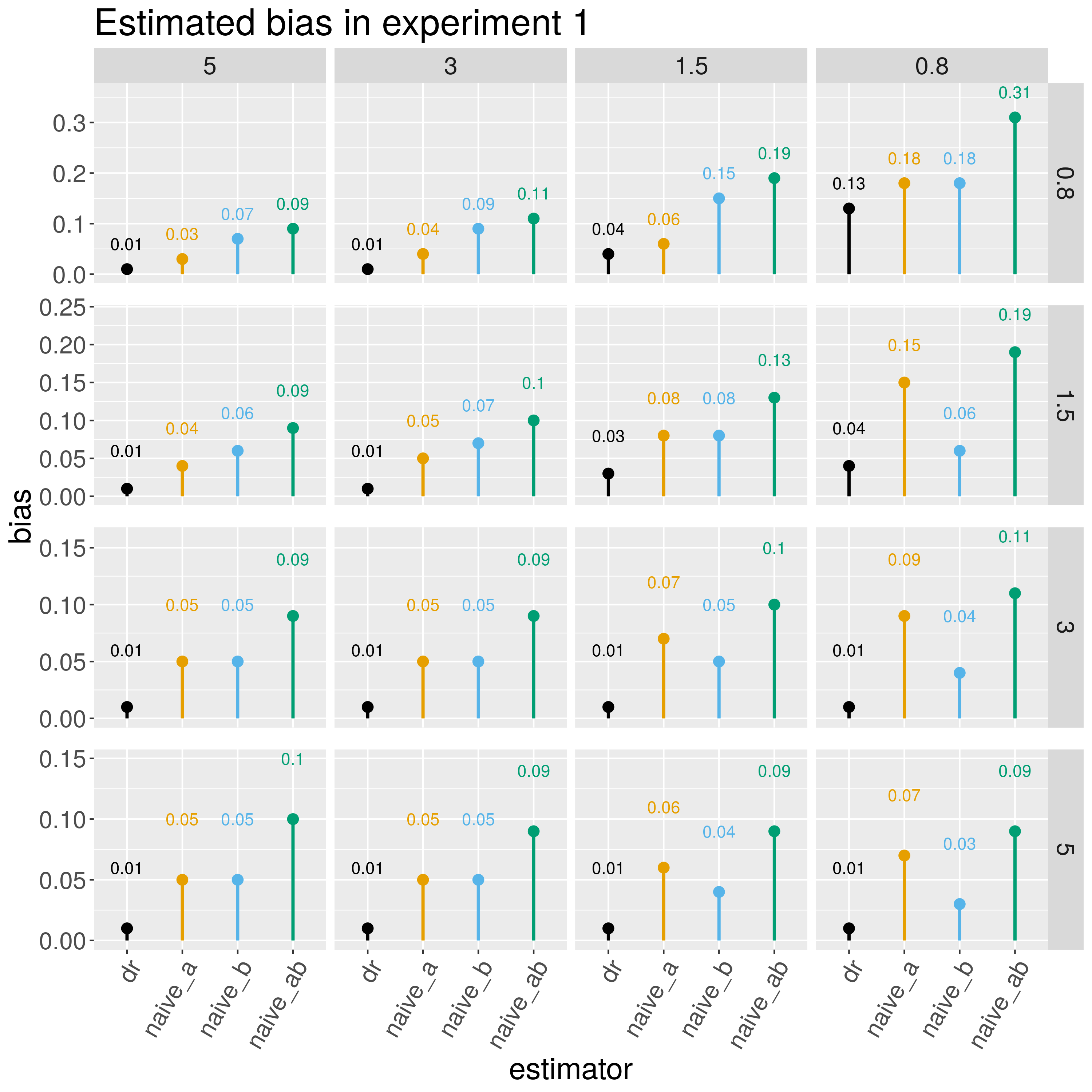
Figure 1: Estimated bias in experiment 1. Rows correspond to different values of $\alpha_{a}$ and columns to different values of $\alpha_{b}$.

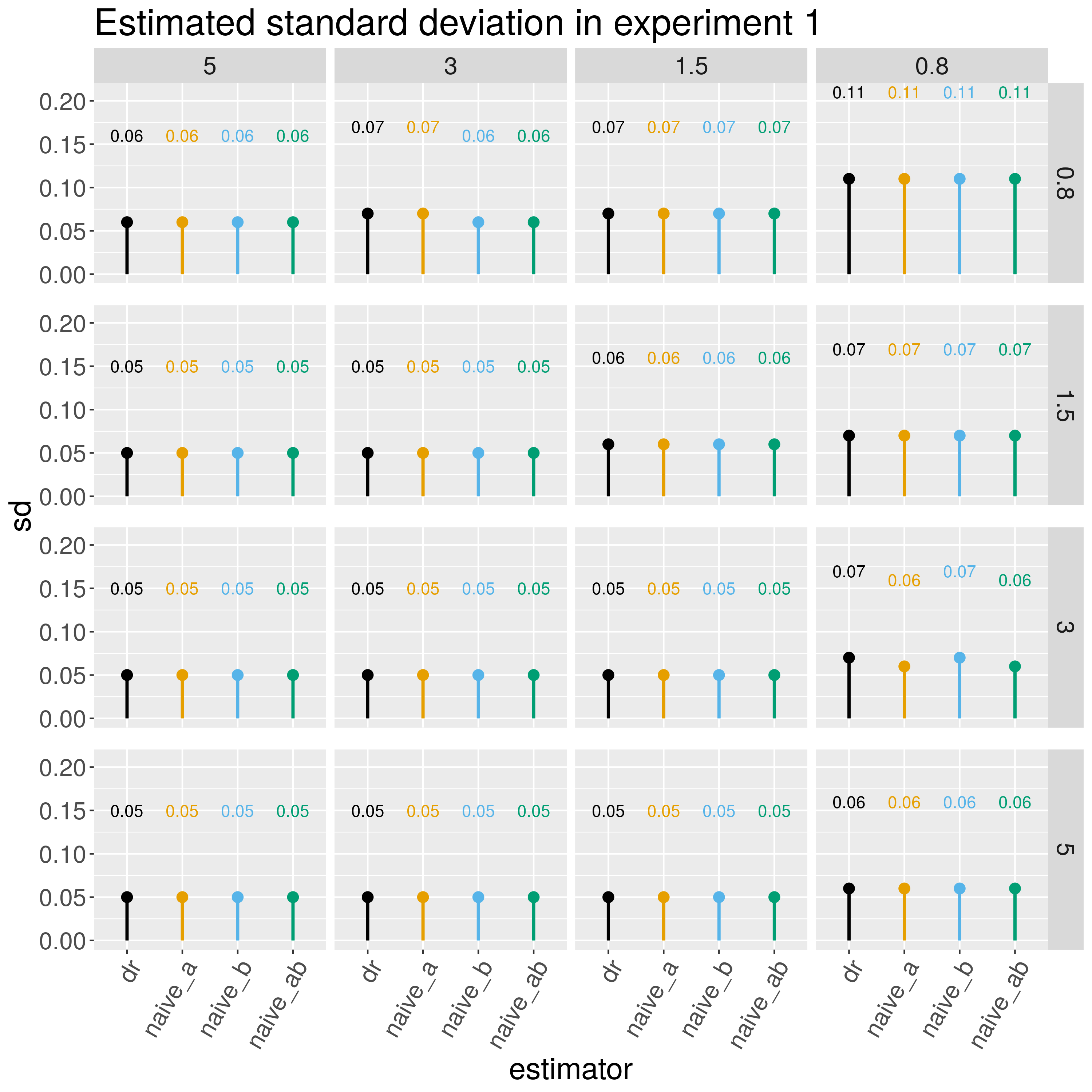
Figure 2: Estimated standard errors in experiment 1. Rows correspond to different values of $\alpha_{a}$ and columns to different values of $\alpha_{b}$.

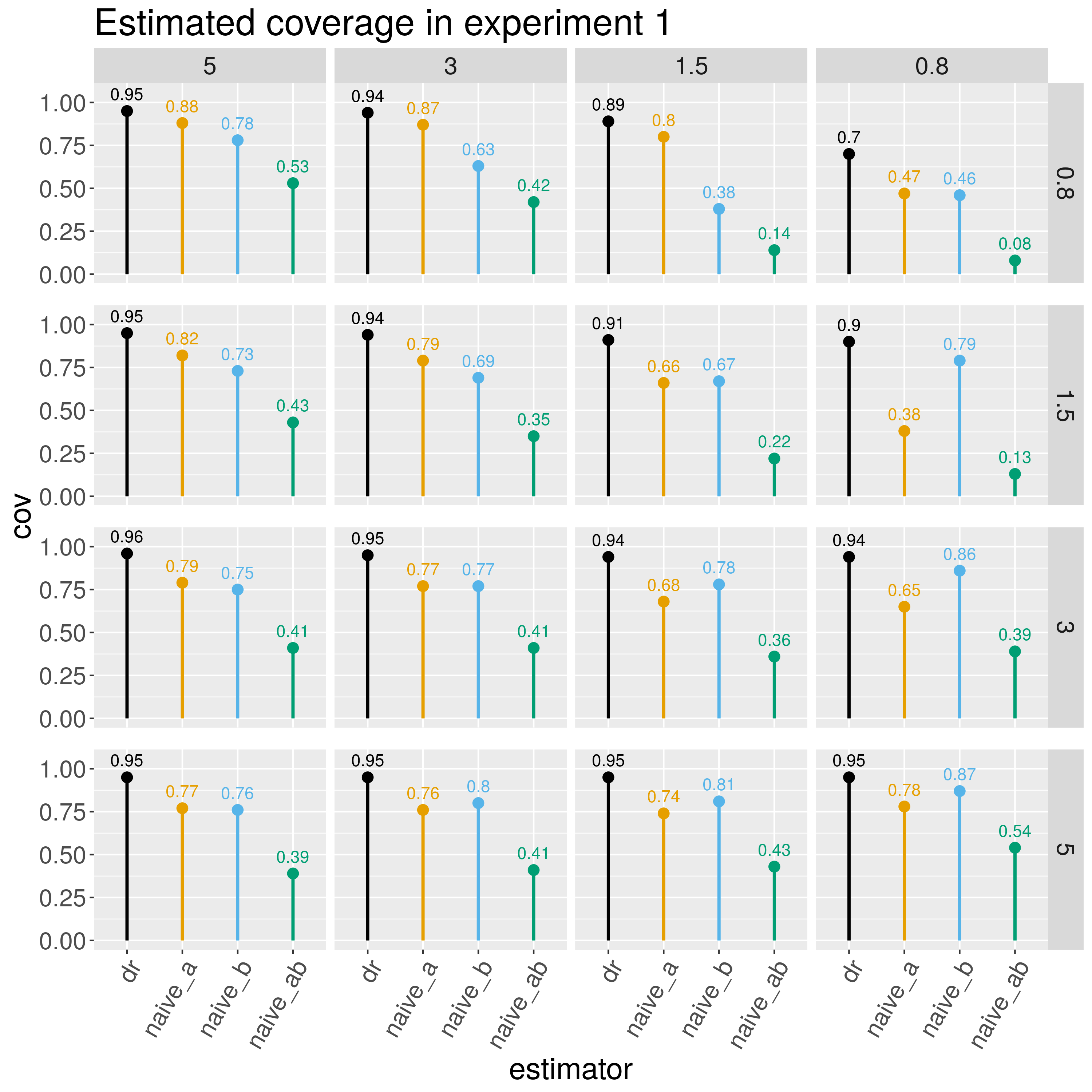
Figure 3: Estimated coverage at the 95% nominal level in experiment 1. Rows correspond to different values of $\alpha_{a}$ and columns to different values of $\alpha_{b}$.

The goal of the second experiment was to study the performance of the estimator in Algorithm 3.1, i.e. when the links of both working models are the identity, and under a scenario in which the model for $a(Z)$ is correctly specified but the model for $b(Z)$ is incorrectly specified. We used $c_{a}=1$, $c_{b}=(\log(3)\theta_{b}^{T}\Sigma\theta_{b})^{-1/2}$ and we generated

$$Y=\langle\theta_{a},Z\rangle+U_{a},$$

$$D|Z\sim Pois(\nu\left(Z\right))\text{ with }\nu\left(Z\right)=\exp(c_{b}\langle\theta_{b},Z\rangle),$$

where $U_{a}$ is normal with $Var(U_{a})=\theta_{a}^{T}\Sigma\theta_{a}/2$.

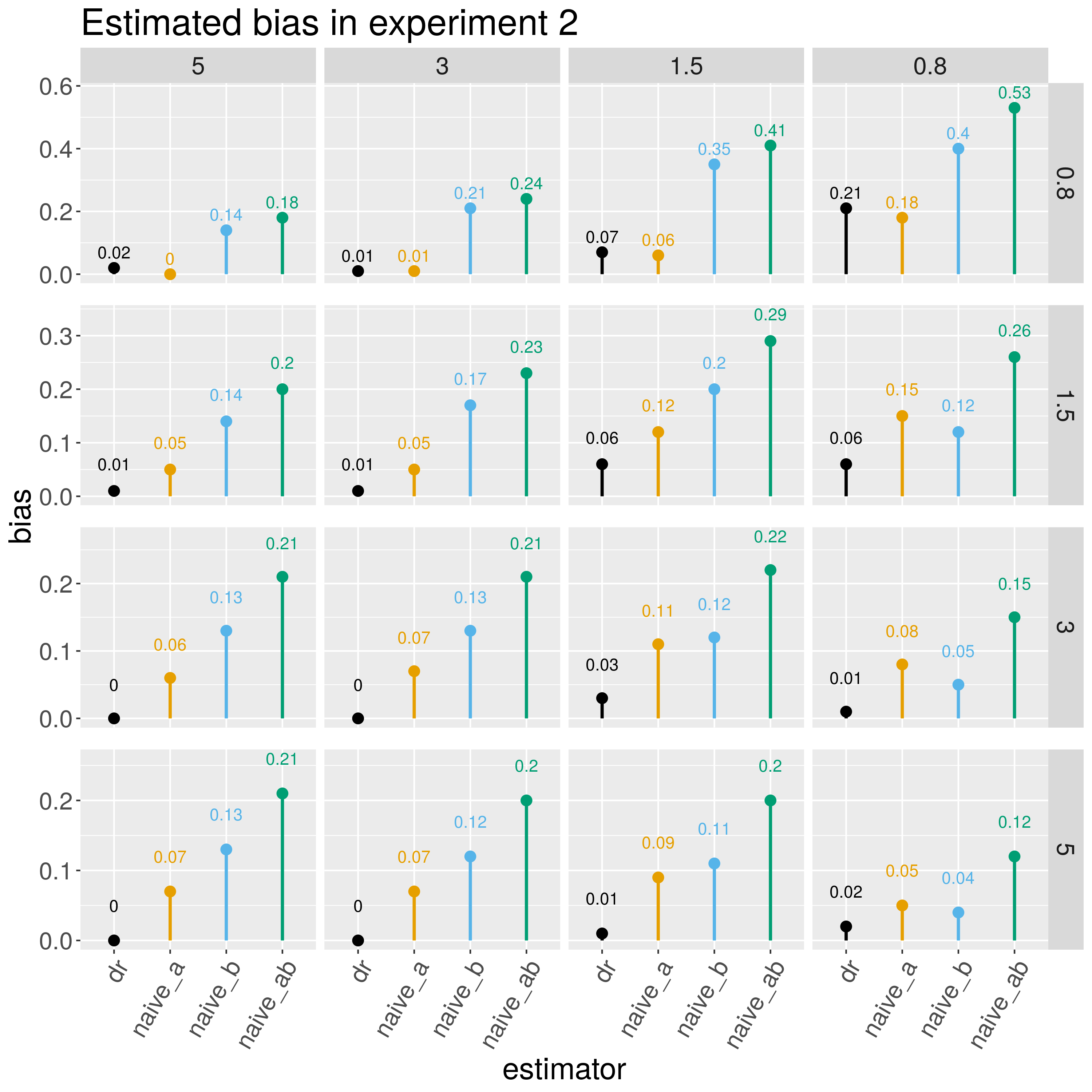
Figure 4: Estimated bias in experiment 2. Rows correspond to different values of $\alpha_{a}$ and columns to different values of $\alpha_{b}$.

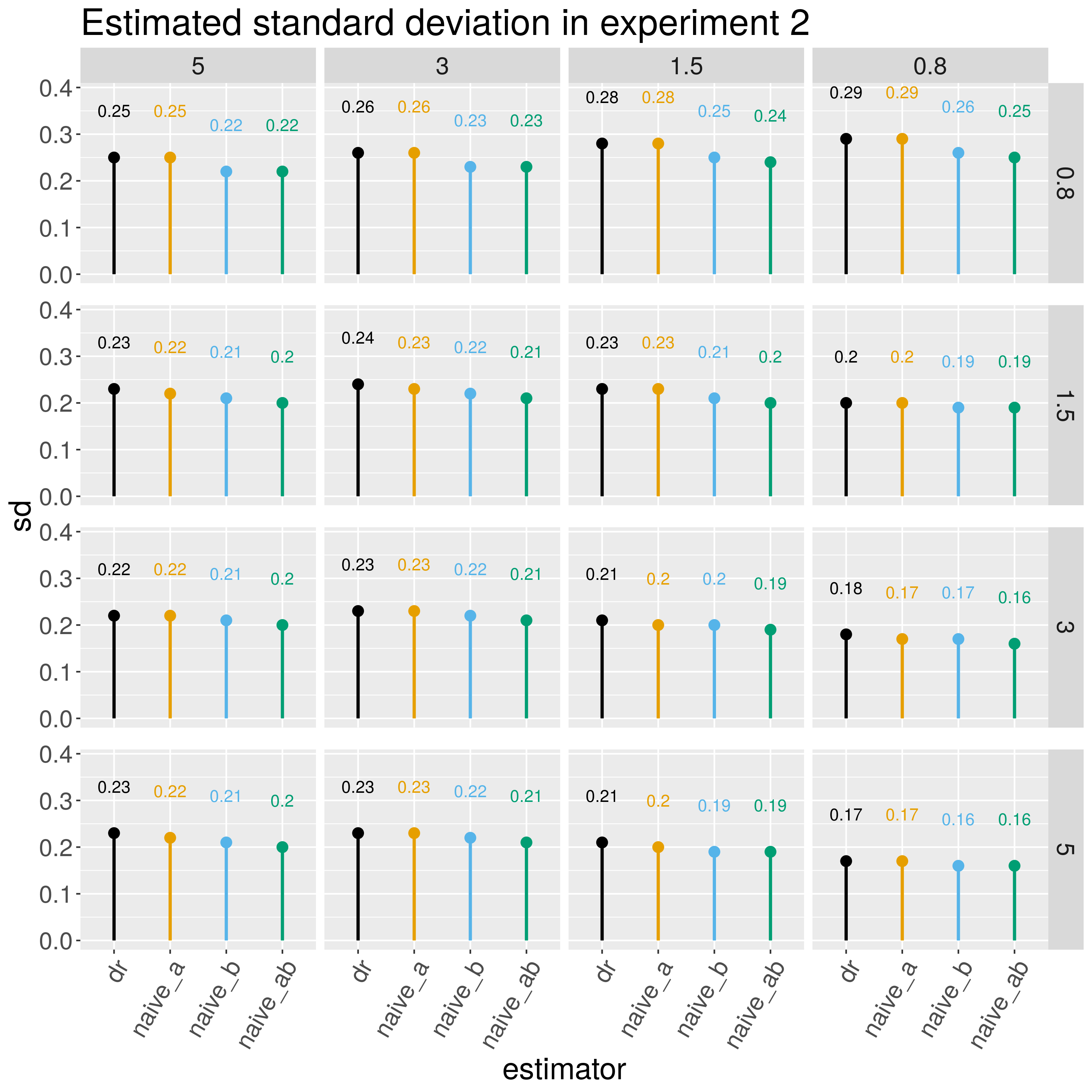
Figure 5: Estimated standard errors in experiment 2. Rows correspond to different values of $\alpha_{a}$ and columns to different values of $\alpha_{b}$.

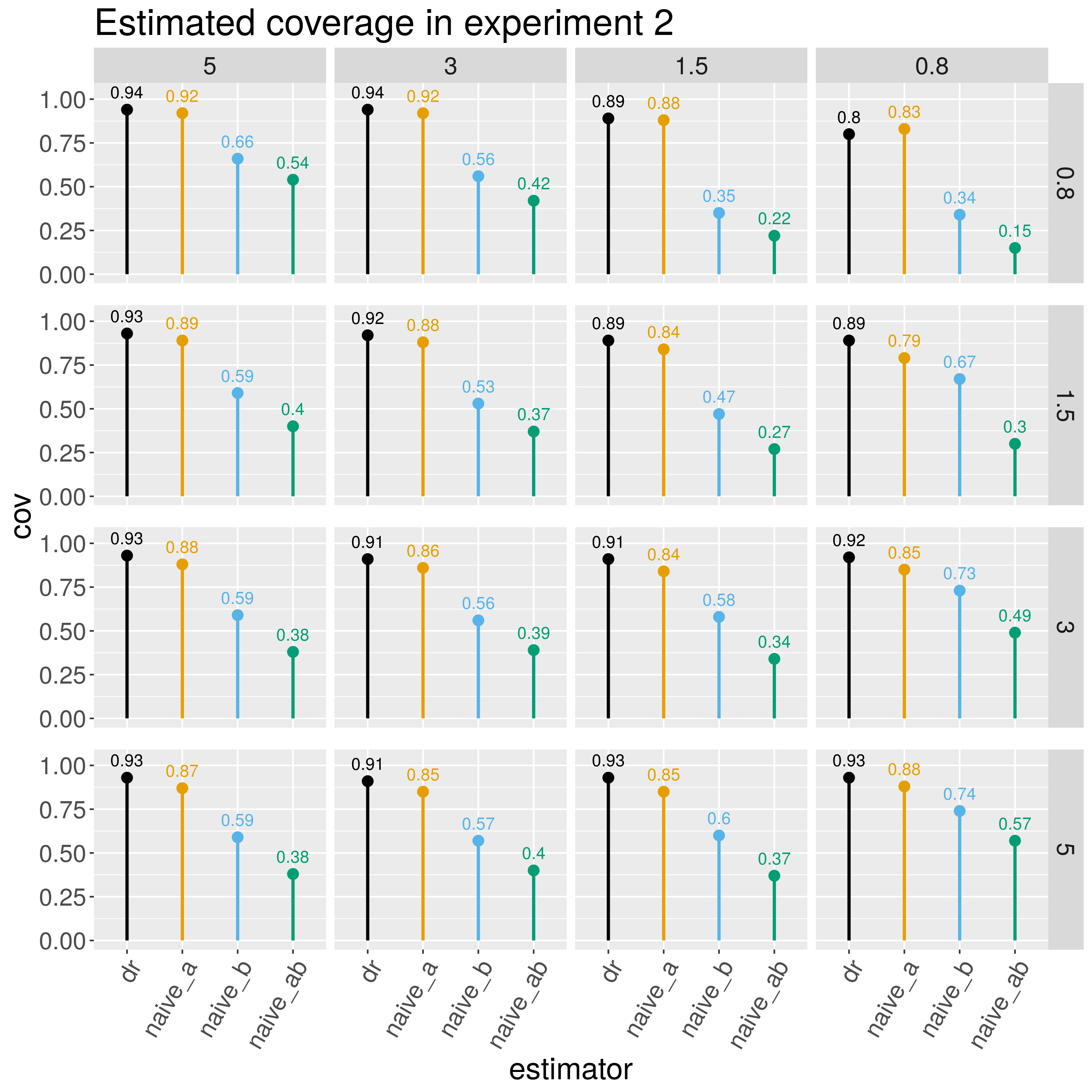
Figure 6: Estimated coverage at the 95% nominal level in experiment 2. Rows correspond to different values of $\alpha_{a}$ and columns to different values of $\alpha_{b}$.

The goal of the third experiment was to study the performance of the estimator in Algorithm 3.2, when the links of both working models are the exponential function, and under a scenario in which both models are correctly specified. We used $c_{a}=(\log(3)\theta_{a}^{T}\Sigma\theta_{a})^{-1/2},$ $c_{b}=(\log(3)\theta_{b}^{T}\Sigma\theta_{b})^{-1/2}$ and we generated $Y$ and $D$ independent given $Z,$ with

$$Y|Z\sim Pois(\nu_{a}\left(Z\right))\text{ with }\nu_{a}\left(Z\right)=\exp(c_{a}\langle\theta_{a},Z\rangle)$$

$$D|Z\sim Pois(\nu_{b}\left(Z\right))\text{ with }\nu_{b}\left(Z\right)=\exp(c_{b}\langle\theta_{b},Z\rangle).$$

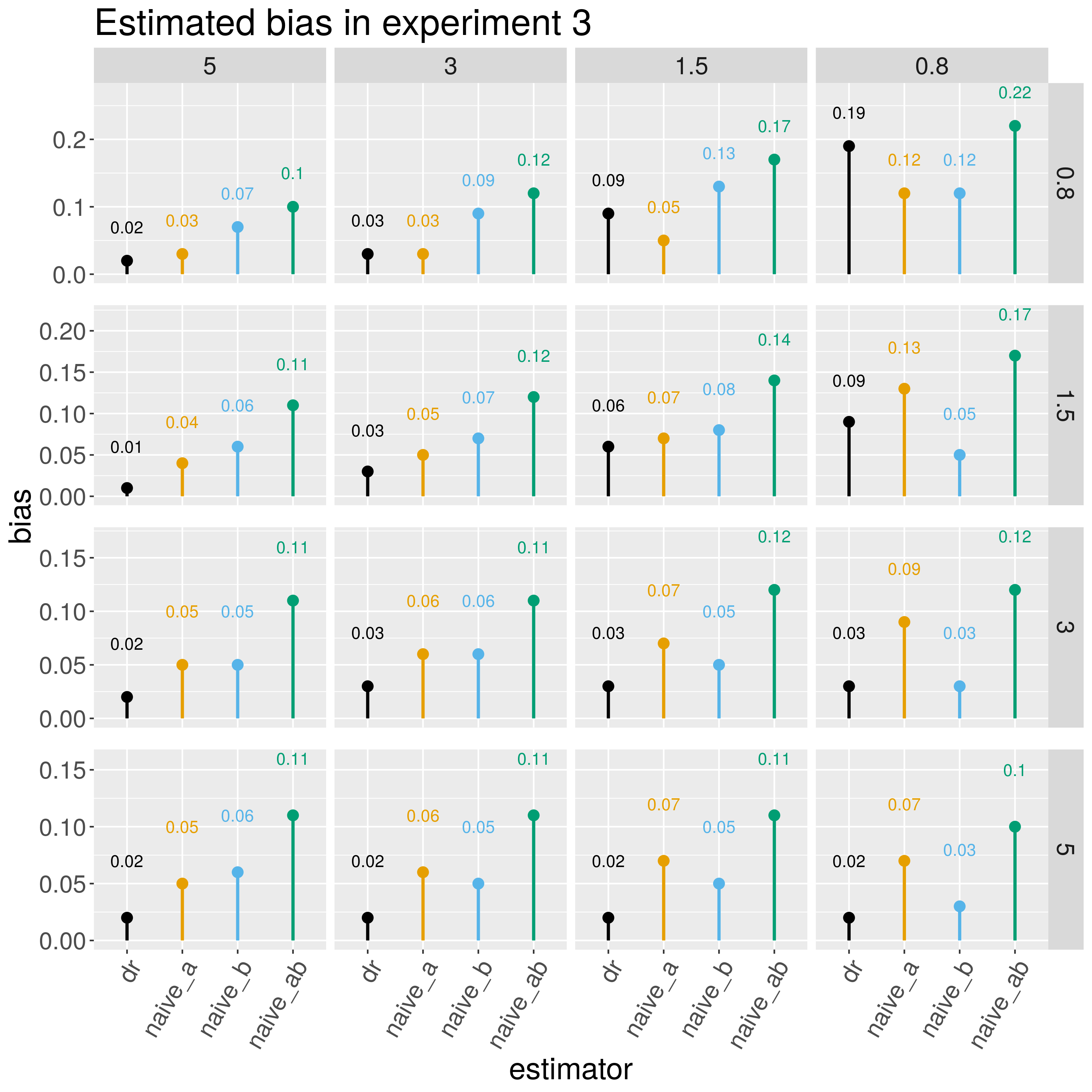
Figure 7: Estimated bias in experiment 3. Rows correspond to different values of $\alpha_{a}$ and columns to different values of $\alpha_{b}$.

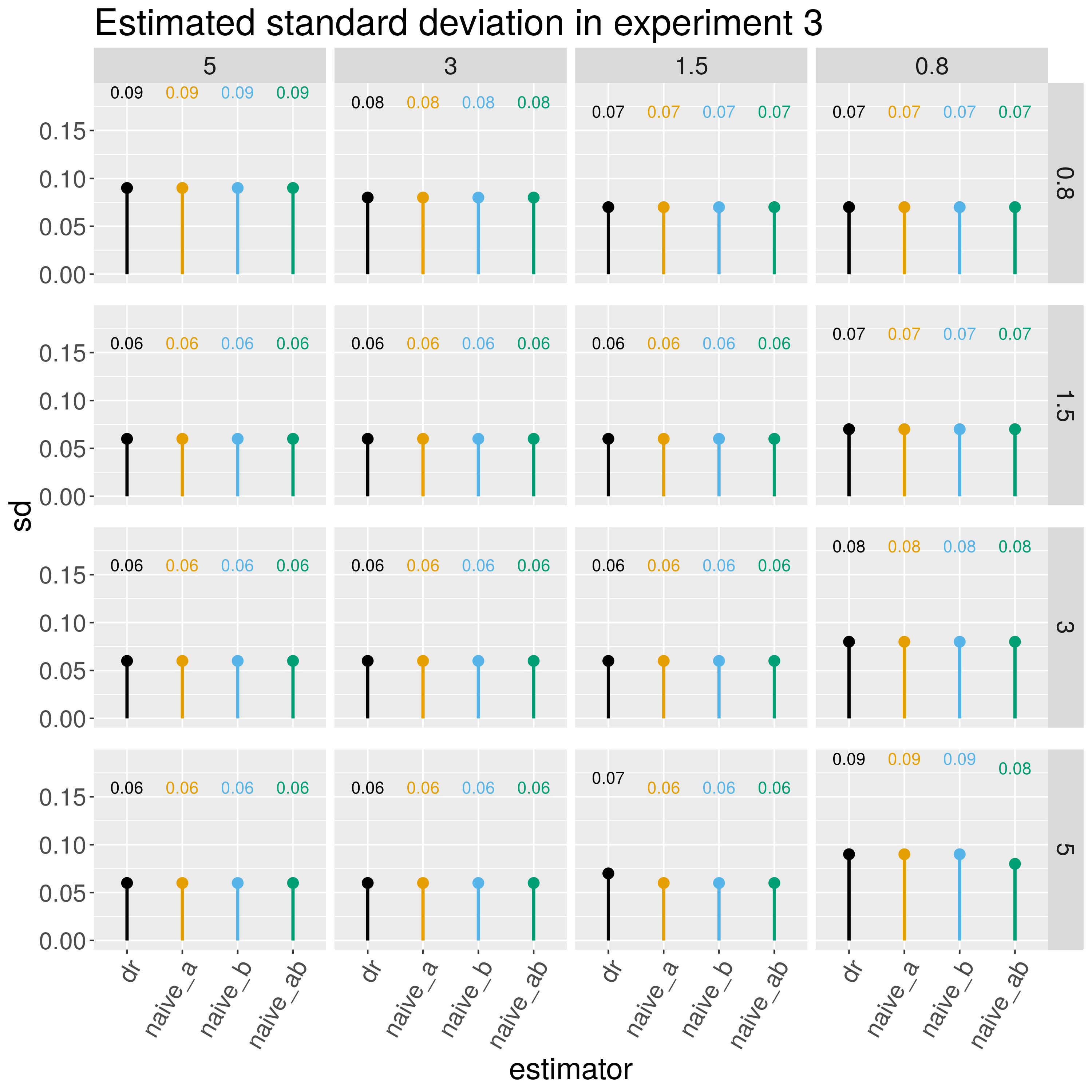
Figure 8: Estimated standard errors in experiment 3. Rows correspond to different values of $\alpha_{a}$ and columns to different values of $\alpha_{b}$.

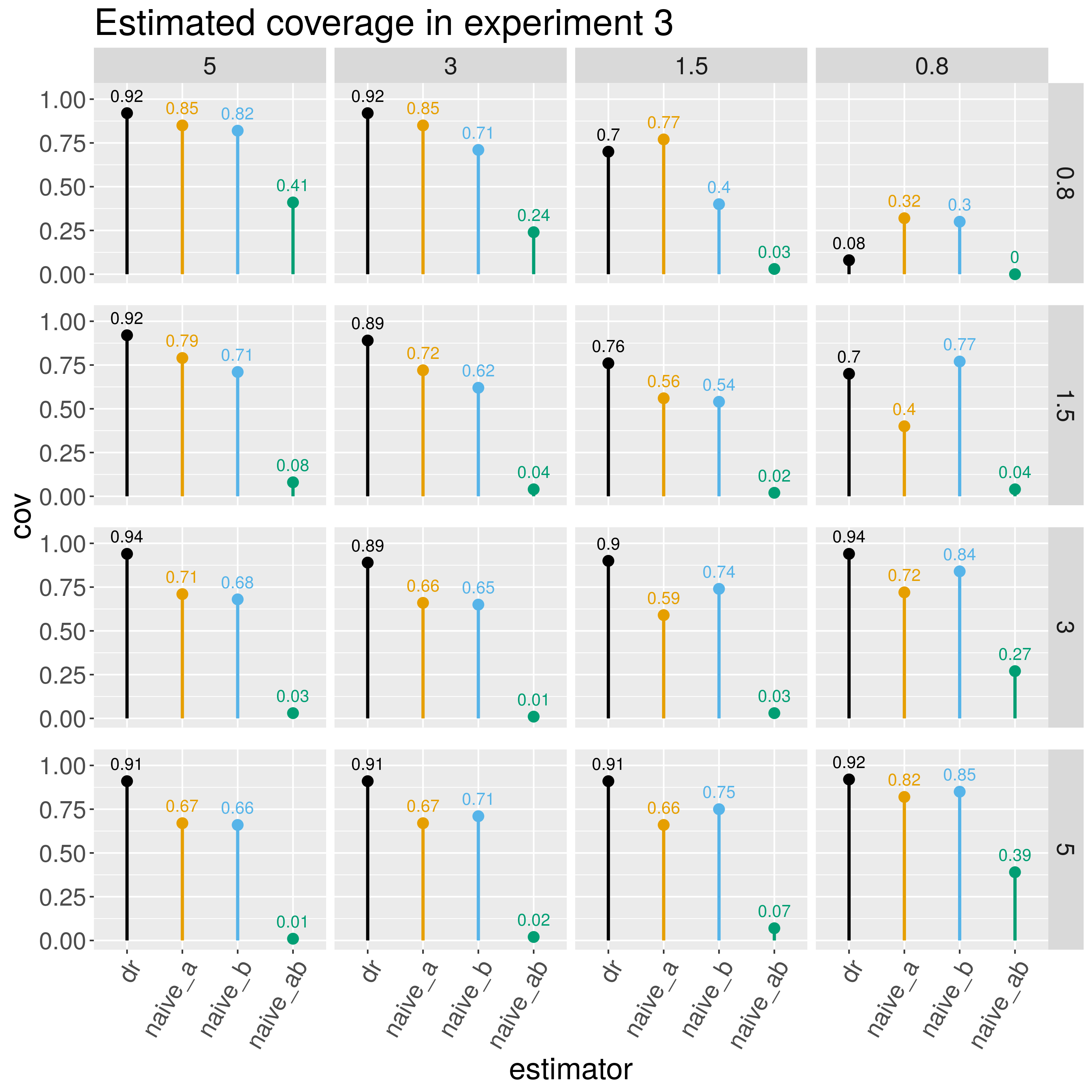
Figure 9: Estimated coverage at the 95% nominal level in experiment 3. Rows correspond to different values of $\alpha_{a}$ and columns to different values of $\alpha_{b}$.

The goal of the fourth experiment was to study the performance of the estimator in Algorithm 3.2, when the links of both working models are the exponential function, and under a scenario in which the model for $a(Z)$ is correctly specified but the model for $b(Z)$ is incorrectly specified. We used $c_{a}=(\log(3)\theta_{a}^{T}\Sigma\theta_{a})^{-1/2},$ $c_{b}=(\theta_{b}^{T}\Sigma\theta_{b})^{-1/2}$ and we generated $Y$ and $D$ independent given $Z,$ with

$$Y|Z\sim Pois(\nu_{a}\left(Z\right))\text{ with }\nu_{a}\left(Z\right)=\exp(c_{a}\langle\theta_{a},Z\rangle)$$

$$D|Z\sim Pois(\nu_{b}\left(Z\right))\text{ with }\nu_{b}\left(Z\right)=(c_{b}\langle\theta_{b},Z\rangle)^{2}.$$

We chose this specific generative process for the law of $D|Z$ so as to roughly satisfy the regularity conditions on the $\ell_{1}$ regularized estimator of $b\left(Z\right)$ of step 2 under an incorrect model. This is because results in Li and Duan, (1989) imply that for large $n,$ this estimator should be close to $\exp\langle\theta_{b}^{L},Z\rangle$ where $\theta_{b}^{L}=Kc_{b}\theta_{b}$ for some constant $K.$ Thus, the coefficients of $\theta_{b}^{L}$ exhibit the same geometric decay as $\theta_{b}.$

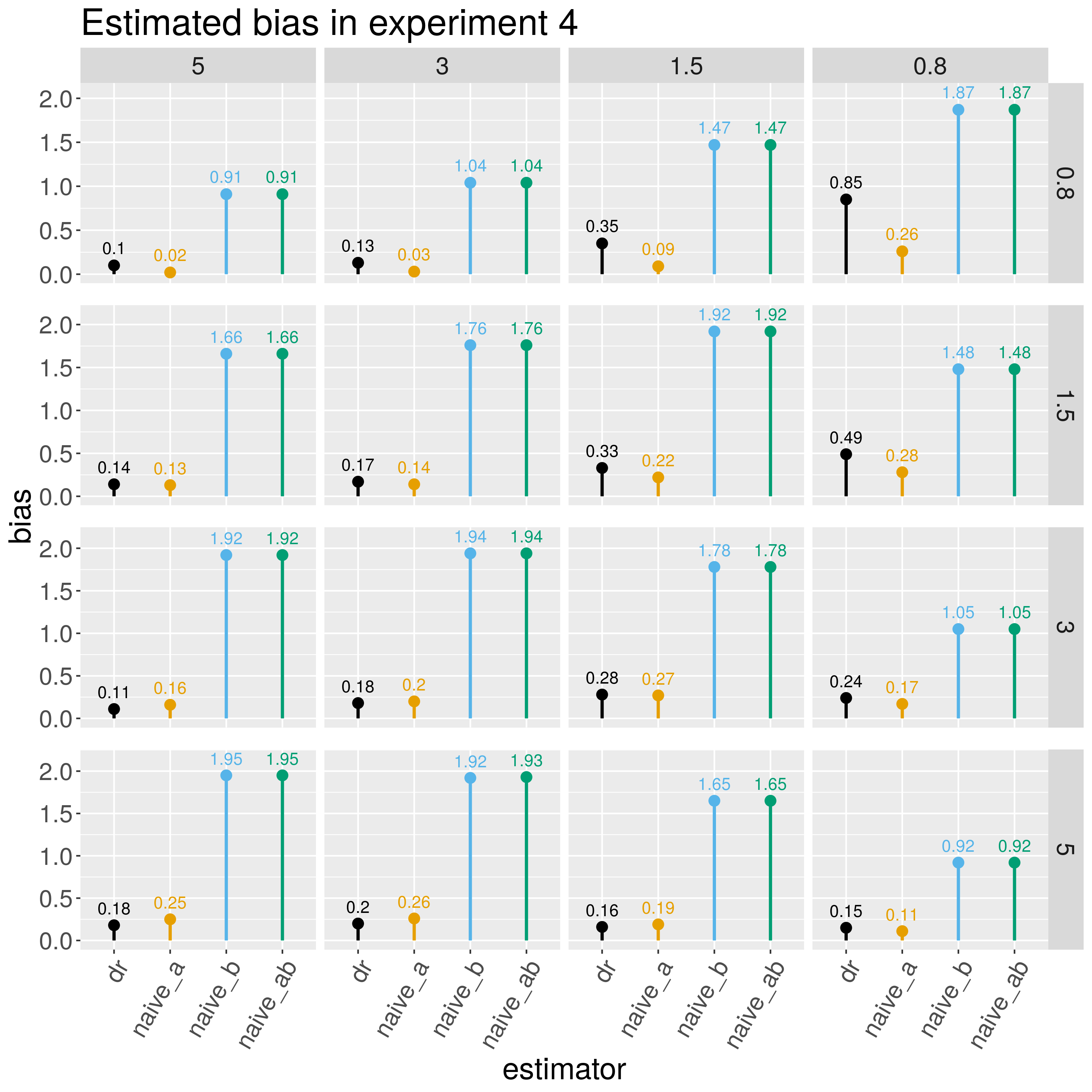
Figure 10: Estimated bias in experiment 4. Rows correspond to different values of $\alpha_{a}$ and columns to different values of $\alpha_{b}$.

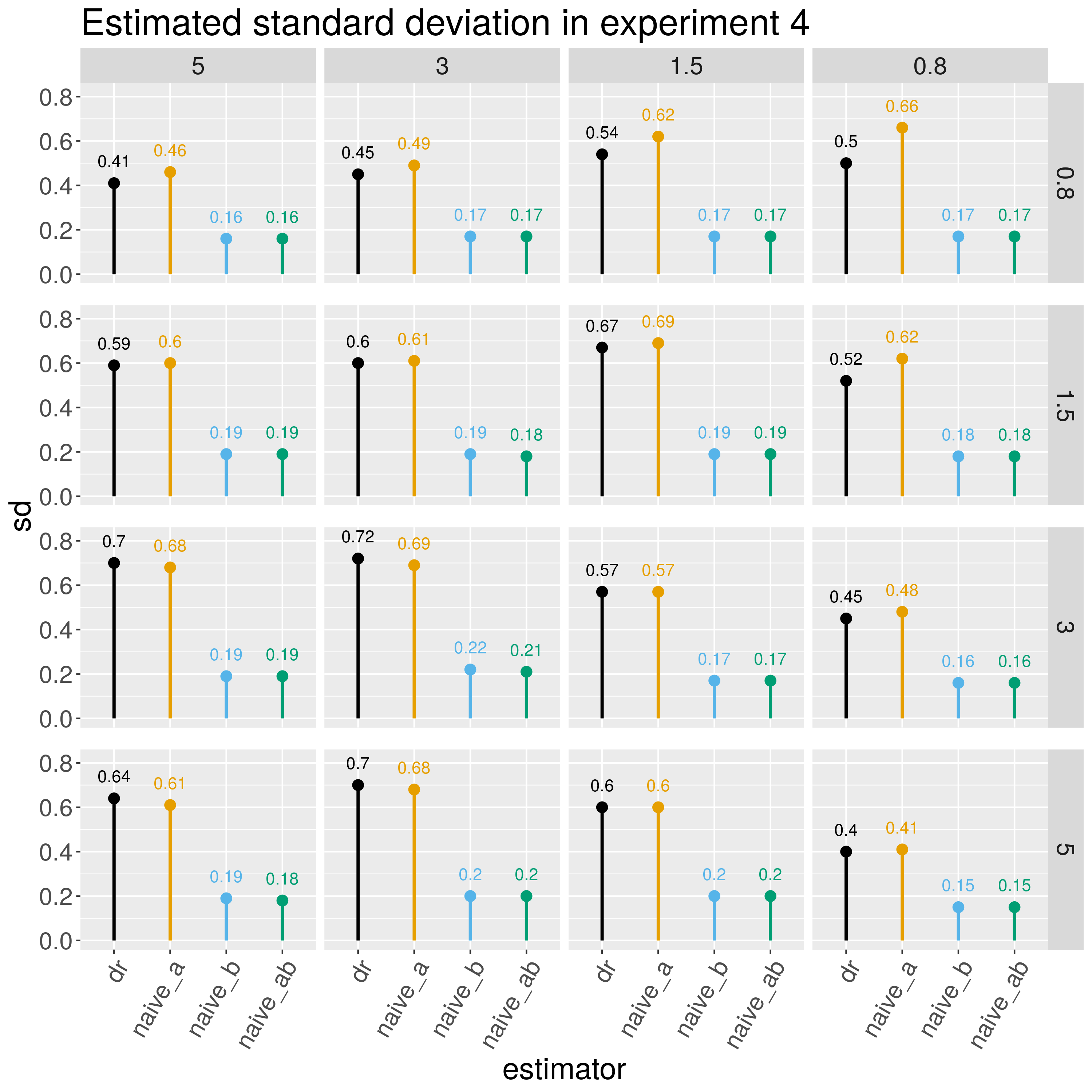
Figure 11: Estimated standard errors in experiment 4. Rows correspond to different values of $\alpha_{a}$ and columns to different values of $\alpha_{b}$.

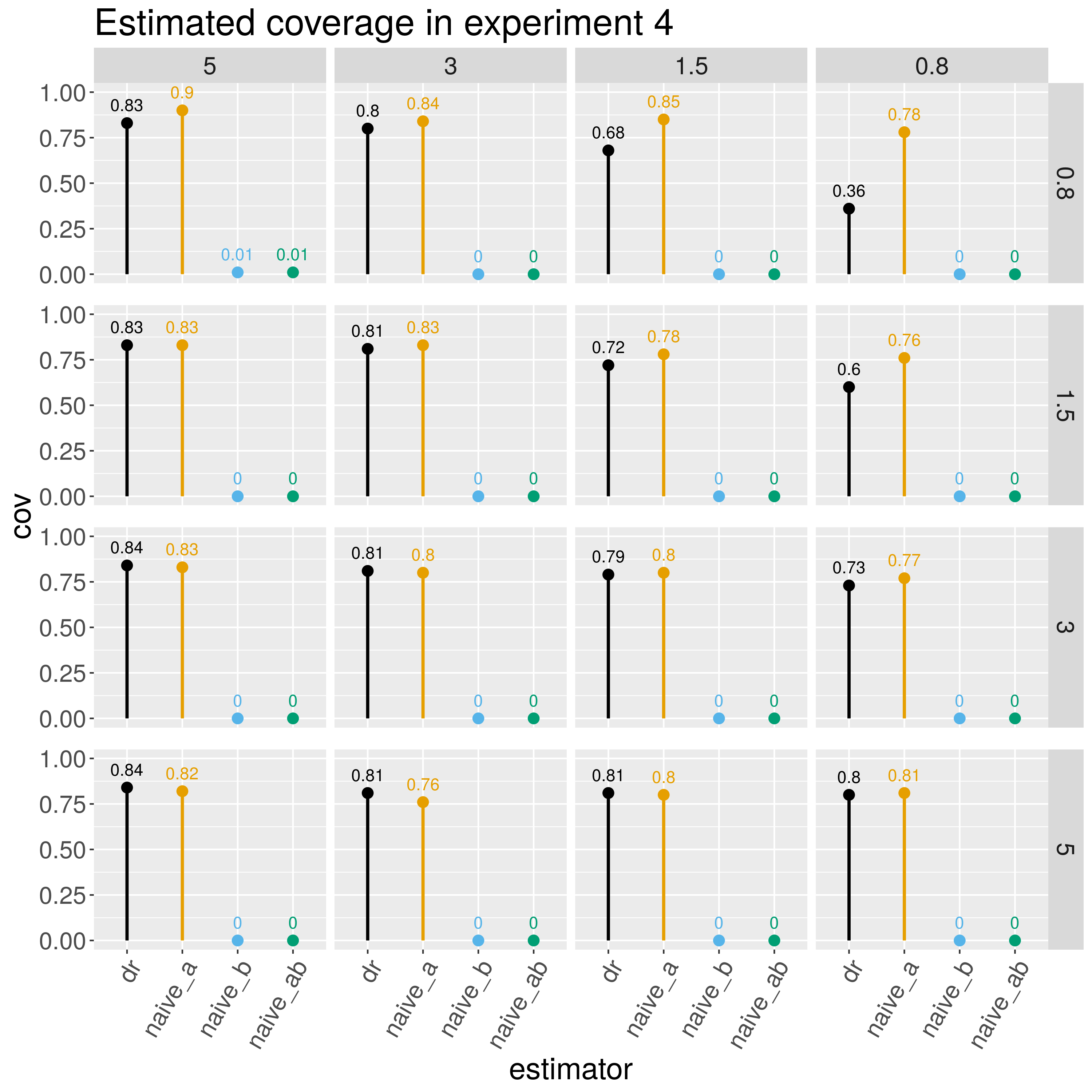
Figure 12: Estimated coverage at the 95% nominal level in experiment 4. Rows correspond to different values of $\alpha_{a}$ and columns to different values of $\alpha_{b}$.

Figures 1-3 and 7-9 show that in experiments 1 and 3, i.e. in the cases in which the working models for $a$ and $b$ are correctly specified, the bias of the doubly robust estimator tends to diminish with increasing values of $\alpha_{a}$ and $\alpha_{b}$. Moreover, the bias of the doubly robust estimator is, for nearly all choices of $\left(\alpha_{a},\alpha_{b}\right)$ is small, relative to its standard error, and much lower than the bias of the naive estimators. The exceptions are the cases

$$\left(\alpha_{a},\alpha_{b}\right)\in\left\{\left(0.8,0.8\right),\left(0.8,1.5\right),\left(1.5,0.8\right)\right\}$$ (84)

and, in experiment 3, also the case $\left(\alpha_{a},\alpha_{b}\right)=\left(1.5,1.5\right).$ In these cases the bias of the DR estimator is of the same magnitude or larger than that of its standard error. Recall that for $\left(\alpha_{a},\alpha_{b}\right)=\left(0.8,0.8\right)$ the key condition $\alpha_{a}^{-1}+\alpha_{b}^{-1}<2$ does not hold and therefore the convergence of our estimators at rate $\sqrt{n}$ is not supported by theory. On the other hand, for the cases $\left(\alpha_{a},\alpha_{b}\right)=\left(1.5,0.8\right)$ and $\left(\alpha_{a},\alpha_{b}\right)=\left(0.8,1.5\right),\alpha_{a}^{-1}+\alpha_{b}^{-1}=1.92,$ and this might reflect the fact that for this borderline case the asymptotic normal approximation is poor. A similar phenomenon might be operating in the case $\left(\alpha_{a},\alpha_{b}\right)=\left(1.5,1.5\right)$ for experiment 3. The coverage probability of the Wald confidence intervals centered at the DR estimators is very close to the nominal 95%, once again, for all choices of $\left(\alpha_{a},\alpha_{b}\right),$ except, as expected, in the aforementioned cases. In contrast, the coverage of the Wald confidence intervals centered at the naive estimators are, for most cases, very poor.

Turn now to experiment 2, i.e. when both working models use linear links, the working model for $a$ is correct but the working model for $b$ is incorrect. Figure 4 shows that in that experiment, the bias of the doubly robust estimator tends to diminish with increasing values of $\alpha_{a}$ and $\alpha_{b}.$ We note that Theorem 4 does not guarantee asymptotic normality of the DR estimator for the case $\alpha_{a}=0.8$ because the key condition of ultra sparsity for the true and correctly modeled function $a$ does not hold. So, the low biases observed for the row corresponding to $\alpha_{a}=0.8\,\$and $\alpha_{b}>0.8$ are not supported by our theoretical results. Also, in experiment 2, Figure 5 shows that the bias of the DR estimator is much smaller than its standard error except for the cases $\left(\ref{eq:alpha_cases}\right)$ and the case $\left(\alpha_{a},\alpha_{b}\right)=\left(1.5,1.5\right).$ For the cases $\left(\alpha_{a},\alpha_{b}\right)=\left(1.5,0.8\right)$ and $\left(\alpha_{a},\alpha_{b}\right)=\left(1.5,1.5\right)$ the poor behaviour of the DR estimator might reflect the fact that the asymptotic theory might be a poor approximation to the finite sample behaviour. The coverages of the confidence intervals centered at the DR estimator are close to the nominal 95% value except for the aforementioned cases.

Finally turn to experiment 4, i.e. when both working models use exponential links, the working model for $a$ is correct but the working model for $b$ is incorrect. Unlike experiment 2, the DR estimator exhibits a somewhat poor behavior, even for the cases in which $\left(\alpha_{a},\alpha_{b}\right)$ satisfy $\alpha_{a}^{-1}+\alpha_{b}^{-1}<2$ and $\alpha_{a}>0.8,$ i.e. cases in which the assumptions of Theorem 4 are satisfied. For instance, when $\left(\alpha_{a},\alpha_{b}\right)=\left(3,1.5\right)$ the bias of the DR estimator is 0.28 which is half its Monte Carlo standard error of 0.57. We suspect that this poor behaviour is, once again, due to the poor approximation of the asymptotic distribution to its finite sample counterpart. This suspicion is supported by the behaviour of the DR estimator when the number of covariates is $p=100$ instead of 200 and $n$ stays equal to 1000. Figures 13-15 report the results of this latter experiment, again based on 500 replications.

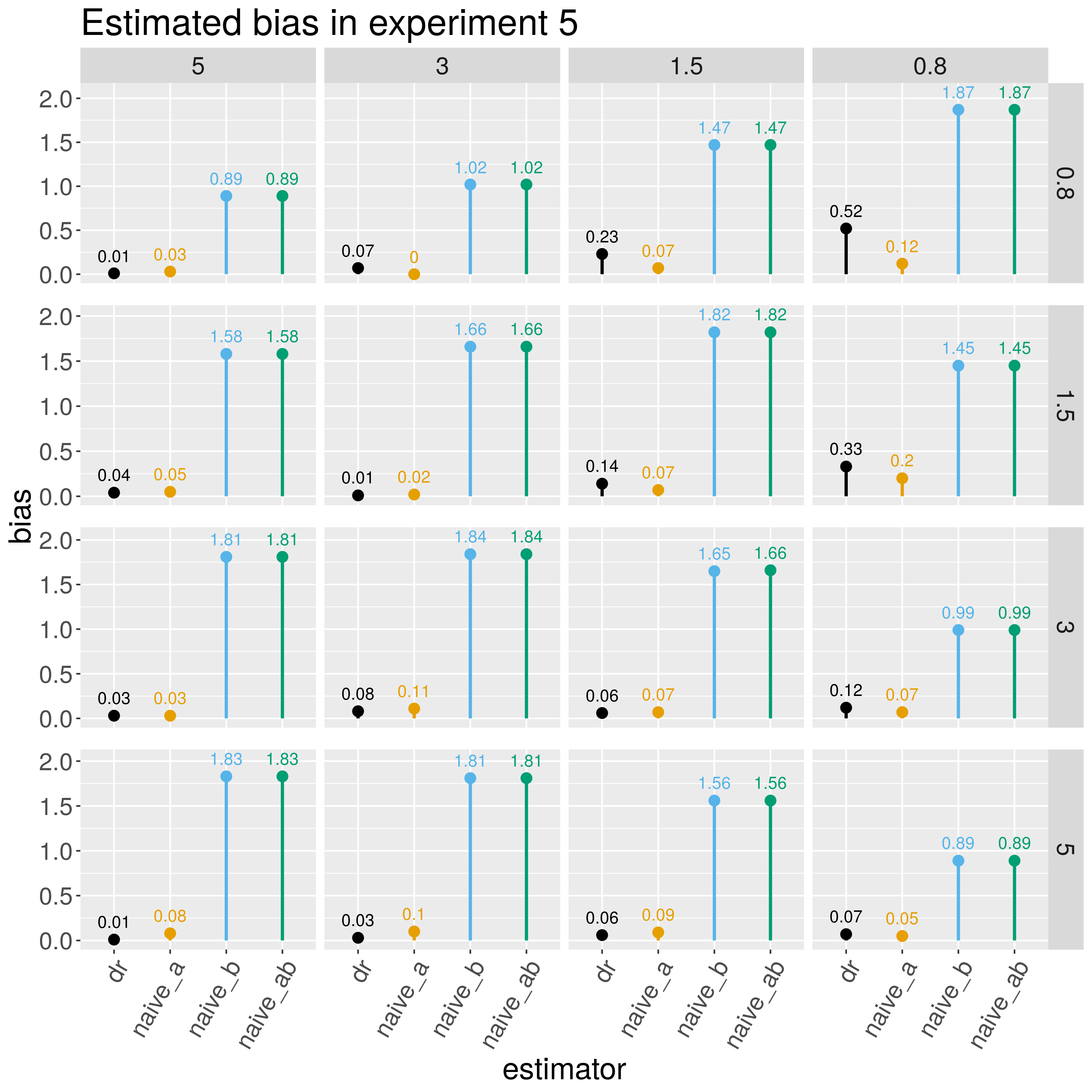
Figure 13: Estimated bias in experiment 5. Rows correspond to different values of $\alpha_{a}$ and columns to different values of $\alpha_{b}$.

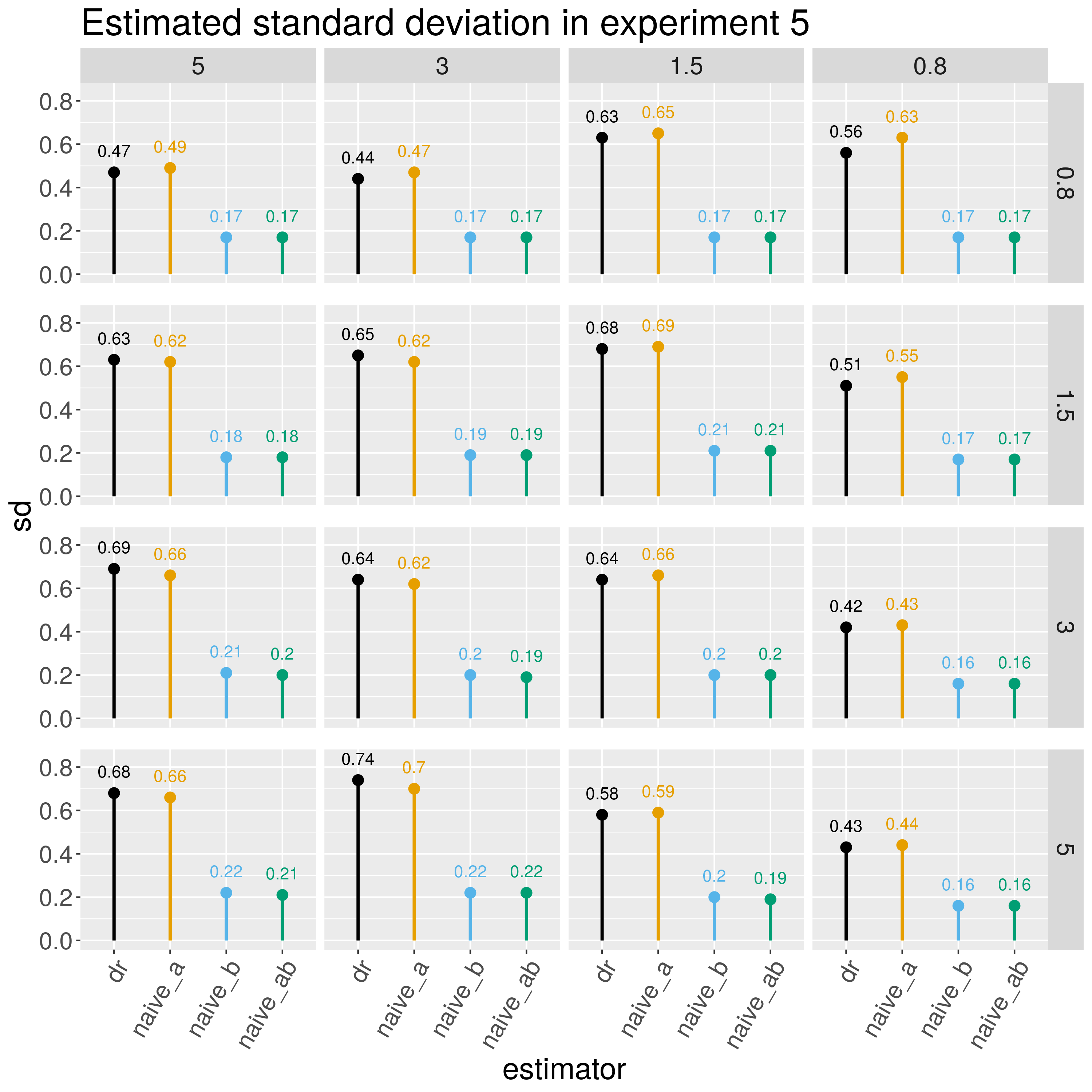
Figure 14: Estimated standard errors in experiment 5. Rows correspond to different values of $\alpha_{a}$ and columns to different values of $\alpha_{b}$.

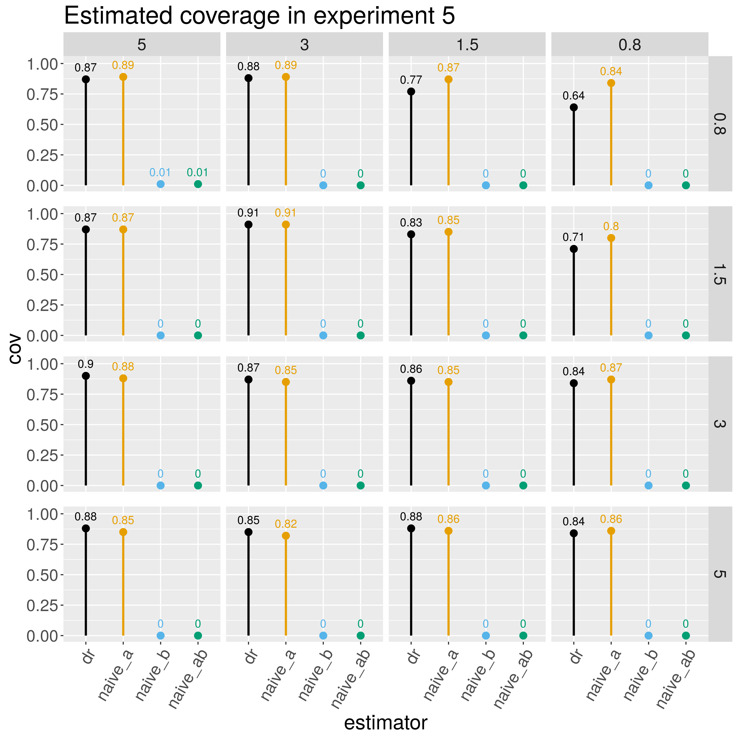
Figure 15: Estimated coverage at the 95% nominal level in experiment 5. Rows correspond to different values of $\alpha_{a}$ and columns to different values of $\alpha_{b}$.

Observe that for this experiment the bias of the DR estimator is orders of magnitude smaller than its standard error. Another concern is the poor coverage probability of the nominal 95% Wald confidence intervals centered at the DR estimator, this problem being more predominant when $p=200$ but also present when $p=100.$ When $p=200$, part of this poor coverage can be attributed in part to the bias of the DR estimator, and also in part to the fact that the standard error estimator underestimates the true standard error. For instance, for a bias that is equal to half the standard error, one would expect the nominal 95% Wald confidence interval to cover with probability roughly equal to 0.92. Yet, when $\left(\alpha_{a},\alpha_{b}\right)=\left(3,1.5\right)$, the bias is half the standard error but the coverage probability is equal to 0.79. A possible explanation for this excess undercoverage is the fact that the mean and median of the estimated standard errors over the 500 replications are equal to 0.51 and 0.45 whereas the Monte Carlo standard error is 0.57. Curiously, in experiment 4, the bias of the ”naive_a” estimator $\mathbb{P}_{n}\left[D\widehat{a}_{N}\left(Z\right)\right]$ is roughly of the same magnitude as the bias of the DR estimator, or even smaller for the scenarios $\left(\ref{eq:alpha_cases}\right)$ and $\left(\alpha_{a},\alpha_{b}\right)=\left(1.5,1.5\right).$ This peculiar behavior of the ”naive_a” estimator was not exhibited in the experiments in which both working models were correctly specified (experiments 1 and 3), so we suspect that it might be due to the specific data generating process that we used in experiment 4. Further investigation of this peculiarity is warranted.

References

- Athey et al., (2018) Athey, S., Imbens, G. W., and Wager, S. (2018). Approximate residual balancing: debiased inference of average treatment effects in high dimensions. Journal of the Royal Statistical Society: Series B (Statistical Methodology), 80(4):597–623.
- Avagyan and Vansteelandt, (2017) Avagyan, V. and Vansteelandt, S. (2017). Honest data-adaptive inference for the average treatment effect under model misspecification using penalised bias-reduced double-robust estimation. arXiv e-prints, page arXiv:1708.03787.
- Ayyagari, (2010) Ayyagari, R. (2010). Applications of influence functions to semiparametric regression models. PhD thesis, Harvard University.
- Belloni and Chernozhukov, (2011) Belloni, A. and Chernozhukov, V. (2011). High dimensional sparse econometric models: An introduction. In Inverse Problems and High-Dimensional Estimation, pages 121–156. Springer.
- Belloni et al., (2015) Belloni, A., Chernozhukov, V., Chetverikov, D., and Kato, K. (2015). Some new asymptotic theory for least squares series: Pointwise and uniform results. Journal of Econometrics, 186(2):345–366.
- Belloni et al., (2014) Belloni, A., Chernozhukov, V., and Hansen, C. (2014). Inference on treatment effects after selection among high-dimensional controls. The Review of Economic Studies, 81(2):608–650.
- Bickel et al., (2009) Bickel, P. J., Ritov, Y., and Tsybakov, A. B. (2009). Simultaneous analysis of lasso and dantzig selector. Ann. Statist., 37(4):1705–1732.
- Bühlmann and Van De Geer, (2011) Bühlmann, P. and Van De Geer, S. (2011). Statistics for high-dimensional data: methods, theory and applications. Springer Science & Business Media.
- Bühlmann and van de Geer, (2015) Bühlmann, P. and van de Geer, S. (2015). High-dimensional inference in misspecified linear models. Electron. J. Statist., 9(1):1449–1473.
- Chan et al., (2016) Chan, K. C. G., Yam, S. C. P., and Zhang, Z. (2016). Globally efficient non-parametric inference of average treatment effects by empirical balancing calibration weighting. Journal of the Royal Statistical Society: Series B (Statistical Methodology), 78(3):673–700.