Planning and Execution of Dynamic Whole-Body Locomotion
for a Hydraulic Quadruped on Challenging Terrain

Abstract

We present a framework for dynamic quadrupedal locomotion over challenging terrain, where the choice of appropriate footholds is crucial for the success of the behaviour. We build a model of the environment on-line and on-board using an efficient occupancy grid representation. We use Any-time-Repairing A* (ARA*) to search over a tree of possible actions, choose a rough body path and select the locally-best footholds accordingly. We run a n-step lookahead optimization of the body trajectory using a dynamic stability metric, the Zero Moment Point (ZMP), that generates natural dynamic whole-body motions. A combination of floating-base inverse dynamics and virtual model control accurately executes the desired motions on an actively compliant system. Experimental trials show that this framework allows us to traverse terrains at nearly 6 times the speed of our previous work, evaluated over the same set of trials.

I Introduction

Agile locomotion is one of the key abilities that legged ground robots need to master. Wheeled or tracked vehicles are efficient in structured environments but can suffer from limited mobility in many real-world scenarios. Legged robots offer a clear advantage in unstructured and challenging terrain. Such environments are common in disaster relief, search & rescue, forestry and construction site scenarios.

This paper presents the newest development in a stream of research that aims to increase the autonomy and flexibility of legged robots in unstructured and challenging environments. We present a framework for dynamic quadrupedal locomotion over highly challenging terrain where the choice of appropriate footholds is crucial for the success of the behaviour. We use perception to build a map of the environment, decide on a rough body path and choose appropriate footholds. We are able to generate feasible footholds on-line and on-board for various types of scenarios such as climbing up and down pallets, traversing stepping stones using an irregular swing-leg sequence and passing over a 35 cm gap. We optimize the body trajectory according to a dynamic stability metric (ZMP) to produce agile and natural dynamic whole-body motions up to $5.8$ times the speed of our previous work [1]. Compliant execution of the motions is performed using a floating-base inverse dynamics controller that ensures the accurate execution of dynamic motions, in combination with a virtual model controller that generates feedback torques to account for model and tracking inaccuracies.

Figure 1: The hydraulically actuated and fully torque controlled quadruped robot HyQ [2]. The inset plot shows the on-line built environment perception alongside with the planned footholds and the current on-board robot state estimate.

Our contribution includes on-line perception, map building and foothold planning, generation and execution of optimized dynamic whole-body motions despite irregular swing-leg sequences and the use of an elegant inverse-dynamics/virtual-model control formulation that exploits the natural partitioning of the robot’s dynamic equations.

The rest of the paper is structured as follows: After discussing previous research in the field of dynamic whole-body locomotion (II) we describe the on-line map building and how appropriate footholds are chosen (III). Section IV explains, how dynamically stable whole-body motions are generated based on an arbitrary footstep sequence. Section V shows how these desired motions are accurately and compliantly executed. In Section VI we evaluate the performance of our framework on the Hydraulic Quadruped robot HyQ (Fig. 1) in real-world experimental trials before Section VII summarizes this work and presents ideas for future work.

II Related Work

In environments where smooth, continuous support is available (flats, fields, roads, etc.), where exact foot placement is not crucial for the success of the behaviour, legged systems can utilize a variety of dynamic gaits, e.g. trotting, galloping. Marc Raibert pioneered the study of the principles of dynamic balancing with legged robots [3], resulting in the quadruped BigDog. The reactive controllers used in these legged systems are partially capable to overcome unstructured terrain. Likewise, HyQ can traverse lightly unstructured terrain using reactive control [4, 5] or reflex strategies [6].

However, for more complex environments with obstacles like large gaps or stairs, such systems quickly reach their limits. In this case, higher level motion planning that considers the environment and carefully selects appropriate footholds is required. In these terrains, e.g. stairs, gaps, cluttered rooms, legged robots have the potential to use non-gaited locomotion strategies that rely more on accurate foothold planning based on features of the terrain. There exist a number of successful control architectures [7, 8, 9, 10] to plan and execute footsteps to traverse such terrain. Some avoid global footstep planning by simply choosing the next best reachable foothold [8], while others plan the complete footstep sequence from start to goal [10], often requiring time consuming re-planning in case of slippage or deviation from the planned path.

The approach in [7] stands between the two above mentioned methods and plans a global rough body path to avoid local minima, but the specific footholds are chosen only a few steps in advance. This reduces the necessary time for re-planning in case of slippage, while still considering a locally optimal plan. We recently built on this approach with a path planning and control framework that uses on-line force-based foothold adaptation to update the planned motion according to the perceived state of the environment during execution [1].

The whole-body locomotion framework described in this paper further extends this work: We use real-time perception to create, evaluate and update a terrain cost map on-board. Compared to previous approaches our framework does not make use of any external state measuring system, e.g. a marker-based tracking system. The incorporation of domain knowledge, e.g. body motion primitives and an ARA* planner, allows us to re-plan actions and footholds on-line. As in [7] the Center of Gravity (CoG) trajectory is now chosen to comply with the ZMP dynamic stability metric [11] to produce agile, fast and natural motions.

III Perception and (Re-)Planning

This section describes the pipeline from the acquisition and evaluation of terrain information to the generation of appropriate footholds (Fig. 2). The on-board terrain information server continuously holds the state of the environment. The body action planner decides the general direction of movement and the footstep sequence planner chooses specific footholds along this path.

Figure 2: An overview of the perception and planning system that generates footstep sequences according to the terrain information.

III-A Terrain Information

We develop a terrain information server that computes the required information for the body action and the footstep sequence planners, e.g. the terrain cost map of the environment. We build a 3D occupancy grid map [13] from a RGBD sensor mounted on a scanning pan & tilt unit, alongside with the state estimate of the robot using the Extended Kalman Filter [14]. The voxel-based map is built using a $(x,y,z)$ resolution of ($4\,\mathrm{cm}\times 4\,\mathrm{cm}\times 2\,\mathrm{cm}$) which roughly matches the dimensions of the robot’s foot.

The terrain cost map quantifies how desirable it is to place a foot at a specific location. The terrain cost $c_{t}$ for each voxel in the map is computed using geometric terrain features as in [1]. Namely, we use the standard deviation of height values, the slope and the curvature of the cell in question. The terrain cost $c_{t}$ for each voxel of the map is computed as a weighted linear combination of the individual features $c_{t}(x,y)=\mathbf{w}^{T}\mathbf{c}(x,y)$. The cost map is locally re-computed (in a 2.5 m$\times$5 m area around the robot) whenever a change in the map is detected.

III-B Body Action Planner

The state ${\mathbf{s}=(x,y,\theta)}\in\mathcal{S}$ of the robot body includes the current position $(x,y)$ and the yaw angle $\theta$. Given a desired goal state, the body action planner finds a sequence of actions $\mathbf{a}_{0\dots N}=\{\mathbf{a}_{0},\mathbf{a}_{1},\dots,\mathbf{a}_{N}\}$ that move the robot in a nearly optimal way to this state. This implies that terrain features, the difficulty of specific actions, kinematic reachability and collision with the environment must be considered and quantified. A feasible action $\mathbf{a}$ is the change of state that can be achieved through one step from $\mathbf{s}$ to $\mathbf{s^{\prime}}$ as

$$\mathbf{a}=(\Delta x,\Delta y,\Delta\theta)\in\mathcal{A}.$$ (1)

We define $\mathcal{A}$ as the set of -empirically chosen- feasible motion primitives (e.g. move left, diagonally forward, back) that correspond to the kinematics and dynamics of the robot. The cost of an action $\mathbf{a}$ given a current state $\mathbf{s}$ is computed as a weighted linear combination of costs:

$$c(\mathbf{s},\mathbf{a})=\mathbf{w}^{T}\mathbf{c}(\mathbf{s},\mathbf{a})$$ (2)

with $\mathbf{c}(\mathbf{s},\mathbf{a})$ consisting of:

$\bar{c}_{t}$

The average of the best n terrain costs around each leg after performing action $\mathbf{a}$.

$c_{a}$

The difficulty of a specific action, e.g. sideways steps are more difficult than forward ones.

$c_{pc}$

Penalizes actions that potentially cause the swing-leg to collide with the environment.

$c_{po}$

Penalizes actions that potentially end up in uneven terrain that require large roll and pitch angles.

The set of actions $\mathcal{A}$ and the current state $\mathbf{s}$ of the robot is used to construct a directed graph $\mathcal{G}=(\mathcal{S},\mathcal{A})$ (Fig. 3).

Figure 3: A sketch of the body action graph. The objective is to find a sequence of actions $\mathbf{a}$ from the current body state ${\mathbf{s}=(x,y,\theta)}$ to the goal state $\mathbf{g}$, that minimizes the accumulated action costs $c(\mathbf{s},\mathbf{a})$. For simplicity only three possible actions are shown, namely move left ($\mathbf{a}^{l}$), right ($\mathbf{a}^{r}$) and forward ($\mathbf{a}^{f}$). The optimal action sequence {$\mathbf{a}^{l},\mathbf{a}^{r},\dots,\mathbf{a}^{r}$} found through ARA* is shown in red.

We use the ARA* [15] algorithm to search the tree for a sequence of actions with the lowest accumulated cost from the current to the goal state. ARA* uses a heuristic $h(\mathbf{s})=-\bar{c}\mathcal{F}(\|\mathbf{g}-\mathbf{s}\|)$ to decide along which states to search first. $\mathcal{F}(\cdot)$ is the estimated remaining steps (actions) to reach the goal state and $\bar{c}$ is an estimated lower bound on the average future action costs, considering the terrain costs between the current and the goal state.

ARA* initially runs an A* search with an inflated heuristic, ${\epsilon\cdot h(s)}$, which quickly finds a first sequence of actions. Unfortunately, since the inflated heuristic is no longer admissible (always lower than the true cost), the sequence of actions may be sub-optimal. As long as computational time is still available, ARA* repeatedly runs A* search, continuously decreasing the inflation factor $\epsilon$ and thereby finding closer to optimal sequences of actions. Since a first solution, although suboptimal, is found quickly, this algorithm can be used online.

III-C Footstep Sequence Planner

Given the desired body action plan, the footstep sequence planner computes the sequence of footholds that corresponds to these body actions. In our previous work, we selected the optimal foothold around the nominal stance positions in a predefined swing-leg sequence. In this paper, we modify the position of the search area and the swing-leg sequence depending on the corresponding action, which improves the robustness of the planned actions. For example, when moving left (action $\mathbf{a}^{l}$) it is advantageous to swing one of the left legs to avoid small areas of support.

The footstep location in each search area with the lowest foothold cost, $c_{f}=w_{t}c_{t}+w_{st}c_{st}+w_{c}c_{c}+w_{o}c_{o}$, is then selected, where $c_{t}$ is the terrain cost below a foothold, $c_{st}$ is the support triangle cost, $c_{c}$ is the leg collision cost and $c_{o}$ is the body orientation cost.

Figure 4: (Re-)planning and perception. The left image shows how a map of the environment is built (cost values in grayscale) along with the body path (green line) and the footstep sequence plan (colored spheres). Once the environments changes the map is updated and the footsteps re-planned.

III-D Re-planning/Updating during Execution

Compared to our previous approach the graph is significantly smaller, since we only search over feasible actions $\mathcal{A}$ and not over every discretized change in state. Additionally, ARA* provides intermediate solutions, so the exhaustive and time-costly search procedure does not need to be completed before the robot can react. This combination of the efficient voxel-based occupancy map, the graph representation over feasible actions, and the efficient search through ARA* allows us to re-plan the motions and set of planned footholds online to cope with changes in the environment as is shown in Fig. 4.

IV Whole-Body Motion Generation

We generate a body trajectory that ensures that the robot is dynamically stable at every time step. We follow the approach presented in [7] that finds a CoG trajectory that respects stability constraints without explicitly generating a ZMP trajectory. We build on this approach by enabling swing-leg sequences in any order through insertion of four-leg support phases.

IV-A Problem Formulation

For a CoG trajectory to be feasible it must be continuous and double differentiable. This way we avoid steps in accelerations that produce discontinuous torques which can damage the hardware and affect stability. The body trajectory, $x_{cog}$, is given by a spline comprised of multiple fifth-order polynomials:

$$x_{cog}(t)=a_{x}t^{5}+b_{x}t^{4}+c_{x}t^{3}+d_{x}t^{2}+e_{x}t+f_{x}.$$ (3)

At each spline junction we require the last state ($t=T_{i}$) of spline $i$ to be equal to the first state ($t=0$) of the next spline $i\!+\!1$ as:

$$(x_{cog},\dot{x}_{cog},\ddot{x}_{cog})_{t=T_{i}}^{i}=(x_{cog},\dot{x}_{cog},\ddot{x}_{cog})_{t=0}^{i+1}.$$ (4)

This ensures double differentiability and continuity of the trajectory, required by the floating-base inverse dynamics. Finding an optimal CoG trajectory can then be reduced to finding optimal polynomial coefficients ${\mathbf{q}_{i}}~{}=~{}(a_{x},\ldots,f_{x},a_{y},\ldots,f_{y})^{T}\in\mathbb{R}^{12}$ for each spline segment $i$.

IV-B Dynamic Stability

To execute the planned footsteps, a body trajectory must be found that ensures a stable stance at all time instances. For slow movements this is achieved by keeping the CoG inside the support polygon, i.e. the polygon formed by the legs in stance. To consider dynamic effects of larger body accelerations we estimate the position of the ZMP by modeling the robot as a cart-table (Fig. 5, left). The ZMP can then be calculated by:

$$x_{zmp}=x_{cog}-\frac{z_{cog}\ddot{x}_{cog}}{\ddot{z}_{cog}+g_{0}},$$ (5)

where $x_{zmp}$ and $x_{cog}$ are the position of the ZMP and the CoG respectively, $z_{cog}$ describes the height of the robot with respect to its feet, $\ddot{z}_{cog}$ is the vertical acceleration of the body and $g_{0}$ represents the gravitational acceleration. Dynamic stability requires the ZMP to be inside the current support triangle, expressed by three lines $l$ of the form $px+qy+r=0$. The ZMP is considered to be inside a support triangle, if the following conditions are met at every sampling interval:

$$p_{l}x_{zmp}+q_{l}y_{zmp}+r_{l}>0\quad\text{ for }l=1,2,3.$$ (6)

In reality there exist discrepancies between the cart-table model and the real robot. Additionally, desired body trajectories cannot be perfectly tracked as modelling, sensing and actuation inaccuracies are hard to avoid. Therefore, it is best to avoid the border of stable configurations by shrinking the support triangles by a stability margin $d$ (Fig. 5, right). With the introduction of $d$, there is no continuous ZMP trajectory when switching between diagonally opposite swing legs as the support triangles are disjoint. We therefore allow a transition period (‘four-leg support phase’) during which the ZMP is only restricted by the shrunk support polygon created by the four stance feet.

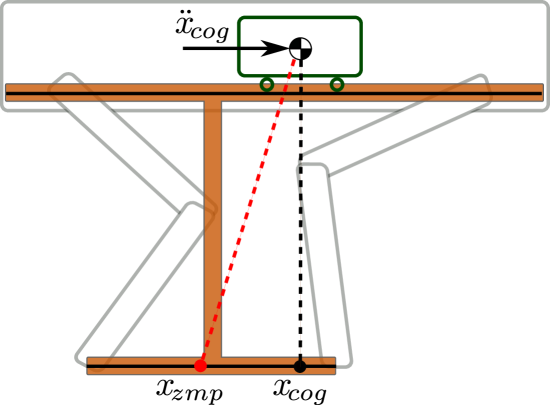
Figure 5: Left: Cart-Table model for representing a quadruped robot: The total mass of the robot is concentrated in the cart that moves on the table. The base of the table represents the current area of support, determined by the current footholds. The ZMP must lie inside this area for dynamic stability. Right: Disjoint support triangles due to the added stability margin $d$. When switching between swinging the left-front (LF) to right-hind (RH) the ZMP must move from the brown to the blue support triangle. Since all four feet are in stance during this phase, the ZMP is only restricted by the red support polygon.

We built on [7] by allowing a completely irregular sequence of steps for the ZMP optimization. Our trajectory generator needs no knowledge of a predefined gait. For every step it checks if the next swing leg is diagonally opposite of the current swing leg. If so, the disjoint support triangles require a four-leg support phase for the optimization to find a solution. This allows a greater decoupling from the footstep planner, which can generate swing leg sequences in any order useful for the success of the behaviour.

IV-C Cost function

In addition to moving in a dynamically stable way, the trajectory should accelerate as little as possible during the execution period $T$. This increases possible execution speed and reduces required joint torques. This is achieved by minimizing

$$J=w_{x}\int_{0}^{T}\!\ddot{x}_{cog}^{2}(t)\,dt+w_{y}\int_{0}^{T}\!\ddot{y}_{cog}^{2}(t)\,dt.$$ (7)

The directional weights $\mathbf{w}$ penalize sideways accelerations ($w_{y}=1.5w_{x}$) more than forward-backward motions, since sideways motions are more likely to cause instability. This results in a convex quadratic program (QP) with the cost function (7), the equality constraints (4) and the inequality constraints (6). We solve it using the freely available QP solver, namely QuadProg++ [16] to obtain the spline coefficients $\mathbf{q}$ and therefore the desired and stable $(x,y)$-body trajectory (3). The remaining degrees of freedom ($z_{cog}$, roll, pitch, yaw) and the swing-leg trajectories are chosen based mostly on the foothold heights and described in detail in [1].

V Execution of Whole-Body Motions

Dynamic whole-body motions require orchestrated and precise actuation of all the joints. Simple PD controllers do not suffice for such motions, especially when considering uncertainties in the environment and/or model inaccuracies. We use a control scheme (Fig. 6) that combines a virtual model with a floating-base inverse dynamics controller.

Figure 6: Pipeline that uses planned footholds to generate dynamic whole-body motions and compliantly executes them using a combination of feedforward and feedback terms.

After receiving an arbitrary sequence of footholds from the footstep planner, the whole-body motion generator calculates desired (feedforward) accelerations $\mathbf{\bm{\ddot{x}}}^{d}$ for the body and a virtual model (VM) control loop adds feedback accelerations $\mathbf{\bm{\ddot{x}}}^{\!f\!b}$ should the robot deviate from the desired trajectory. The inverse dynamics produce the majority of the joint torques which are combined with a low-gain joint-space PD controller to compensate for possible model inaccuracies. The computed reference torques are then tracked by the low-level torque controller. Note that $\mathbf{\bm{x}}$ describes the linear and rotational coordinates of the body as

$$\mathbf{\bm{x}}=(\mathbf{\bm{x}}_{cog},\mathbf{\bm{R}}_{b}),\mathbf{\bm{\dot{x}}}=(\mathbf{\bm{\dot{x}}}_{cog},\mathbf{\bm{\omega}}_{b}),\mathbf{\bm{\ddot{x}}}=(\mathbf{\bm{\ddot{x}}}_{cog},\mathbf{\bm{\dot{\omega}}}_{b}),$$ (8)

where $\mathbf{\bm{R}}_{b}\in\mathbb{R}^{3\times 3}$ is a coordinate rotation matrix representing the orientation of the base w.r.t. the world frame and $\mathbf{\bm{\omega}}_{b}\in\mathbb{R}^{3}$ is the angular velocity of the base.

V-A Virtual Model

The feedback action which compensates for inaccurate execution and drift can be imagined as virtual springs and dampers attached to the robot’s trunk on one side and the desired body trajectory on the other [17]. Deviation between these causes the springs and dampers to produce virtual forces $\mathbf{\bm{F}}_{vm}$ and torques $\mathbf{\bm{T}}_{vm}$ on the body that “pull” the robot back into the desired state through

$$\mathbf{\bm{F}}_{vm}=\mathbf{\bm{P}}_{x}(\mathbf{\bm{x}}_{cog}^{d}-\mathbf{\bm{x}}_{cog})+\mathbf{\bm{D}}_{x}(\mathbf{\bm{\dot{x}}}_{cog}^{d}-\mathbf{\bm{\dot{x}}}_{cog})$$ (9)

$$\mathbf{\bm{T}}_{vm}=\mathbf{\bm{P}}_{\theta}e(\mathbf{\bm{R}}_{b}^{d}\mathbf{\bm{R}}_{b}^{\top})+\mathbf{\bm{D}}_{\theta}(\mathbf{\bm{\omega}}_{b}^{d}-\mathbf{\bm{\omega}}_{b}),$$

where the superscript $d$ refers to the desired values, planned by the whole-body motion generator and non-superscript values describe the state of the robot as estimated by the on-board state estimator. Respectively, $e(.):\mathbb{R}^{3\times 3}\rightarrow\mathbb{R}^{3}$ is a mapping from a rotation matrix to the associated rotation vector [18]. $\mathbf{\bm{P}}_{x},\mathbf{\bm{D}}_{x},\mathbf{\bm{P}}_{\theta},\mathbf{\bm{D}}_{\theta}\in\mathbb{R}^{3\times 3}$ are positive-definite diagonal matrices of proportional and derivative gains, respectively. Expressing the body feedback action in terms of forces and moments allows us give the virtual model gains a physical meaning of stiffness and damping and thus can be intuitively set and used.

Since the inverse dynamics computation requires reference accelerations, we multiply the forces/moments (wrench) $\mathbf{\bm{\mathcal{W}}}_{vm}=(\mathbf{\bm{F}}_{vm},\mathbf{\bm{T}}_{vm})$ with the inverse of the composite rigid body inertia $\mathbf{\bm{I}}_{c}$ of the robot at its current configuration. Adding this body feedback acceleration to the desired body acceleration produced by the whole-body motion generator creates the 6D reference acceleration (linear and rotational) for the inverse dynamics computation as:

$$\mathbf{\bm{\ddot{x}}}^{ref}=\mathbf{\bm{\ddot{x}}}^{d}+I_{c}^{-1}\mathbf{\bm{\mathcal{W}}}_{vm}.$$ (10)

By combining a feedforward acceleration $\mathbf{\bm{\ddot{x}}}^{d}$ with a body-feedback acceleration, we achieve accurate tracking while maintaining a compliant behaviour.

V-B Floating Base Inverse Dynamics

The floating base inverse dynamics algorithm calculates the joint torques required to execute the reference body accelerations. We can partition [19] the dynamics equation of the robot into the unactuated base coordinates $q_{b}\in\mathbb{R}^{6}$ and the active joints’ $q\in\mathbb{R}^{12}$ as

$$\underbrace{\mathbf{\bm{M}}(\mathbf{\bm{R}},\mathbf{\bm{q}})\begin{bmatrix}\mathbf{\bm{\ddot{q}}}_{b}\\ \mathbf{\bm{\ddot{q}}}\end{bmatrix}+\begin{bmatrix}\mathbf{\bm{h}}_{b}\\ \mathbf{\bm{h}}_{q}\end{bmatrix}(\mathbf{\bm{R}},\mathbf{\bm{q}},\mathbf{\bm{\omega}},\mathbf{\bm{\dot{q}}})}_{\mathbf{\bm{b}}}=\begin{bmatrix}\mathbf{\bm{0}}\\ \mathbf{\bm{\tau}}\end{bmatrix}+\begin{bmatrix}\mathbf{\bm{J}}_{cb}^{T}\\ \mathbf{\bm{J}}_{cq}^{T}\end{bmatrix}\mathbf{\bm{\lambda}},$$ (11)

where $\mathbf{\bm{M}}$ is the floating base mass matrix, $\mathbf{\bm{h}}=(\mathbf{\bm{h}}_{b},\mathbf{\bm{h}}_{q})$ is the force vector that accounts for Coriolis, centrifugal, and gravitational forces, $\mathbf{\bm{\lambda}}$ are the ground contact forces, and their corresponding Jacobian $\mathbf{\bm{J}}_{c}=\begin{bmatrix}\mathbf{\bm{J}}_{cb}&\mathbf{\bm{J}}_{cq}\end{bmatrix}$ and $\mathbf{\bm{\tau}}$ are the torques that we wish to calculate.

The left hand term $\mathbf{\bm{b}}=(\mathbf{\bm{b}}_{b},\mathbf{\bm{b}}_{q})$ can be computed efficiently using the Featherstone implementation of the Recursive Newton-Euler Algorithm (RNEA) [20]. Since the CoG acceleration $\mathbf{\bm{\ddot{x}}}_{cog}^{ref}$ is defined in a frame aligned with the base frame but with the origin in the CoG, we perform a translational coordinate transform ${}_{b}\mathbf{\bm{X}}_{cog}$ to get the 6D base spatial acceleration: $\mathbf{\bm{\ddot{q}}}_{b}=\,_{b}\mathbf{\bm{X}}_{cog}\mathbf{\bm{\ddot{x}}}^{ref}$ as in [20].

By partitioning the dynamics equation as in (11) and given that the base is not actuated, we can directly compute, in a least-squares way, the vector of ground reaction forces $\mathbf{\bm{\lambda}}$ from the first $n_{b}$ equations, $\mathbf{\bm{\lambda}}=\mathbf{\bm{J}}_{cb}^{+}\mathbf{\bm{b}}_{b}$, where $()^{+}$ denotes the Moore-Penrose generalized inverse. We then use the last $n$ equations to produce the reference joint torques, $\mathbf{\bm{\tau}}^{id}=\mathbf{\bm{b}}_{q}-\mathbf{\bm{J}}_{cq}^{T}\mathbf{\bm{\lambda}}$.

VI Experimental Results

This section describes the experiments conducted to validate the effectiveness and quantify the performance of our framework.

VI-A Experimental Setup

We use the hydraulically-actuated quadruped robot HyQ in our experiments. HyQ weighs approximately 90 kg, is fully-torque controlled and equipped with precision joint encoders, a depth camera (Asus Xtion) and an Inertial Measurement Unit (MicroStrain). We perform on-board state estimation and do not make use of any external state measuring system, e.g. a marker-based tracking system. All computations are done on-board, using a PC104 stack for the real-time critical part of the framework, and a commodity i7/2.8 GHz PC for perception and planning.

The first experiment starts with flat, obstacle-free terrain. After the robot has planned initial footsteps, a pallet is placed into the terrain. In the next experiments the robot must climb one and two pallets of dimensions 1.2 m $\times$ 0.8 m $\times$ 0.15 m. The height of one pallet is equal to 20% of the leg length. Furthermore we show that the robot traverses a gap of 35 cm, which is approximately half the robot’s body length. The final experiment consist of two pallets connected by a sparse path of stepping stones. The pallets are 1.2 m apart and the stepping stones lie 0.08 m lower than the pallets.

For each experiment, we specify the $(x,y,\theta)$ goal state. The footstep planner finds a sequence of footsteps of an arbitrary order, which the controller then executes dynamically. We validate the performance of our framework in 4 scenarios as seen in Fig. 7 and compare it to our previously achieved results (Table I) on the same benchmark tasks. Additionally, the reader is strongly encouraged to view the accompanying video as it provides the most intuitive way to demonstrate the performance of our framework.

VI-B Results and Discussion

Figure 7: Snapshots of experimental trials used to evaluate the performance of our framework. From top to bottom: crossing a 15 cm pallet; climbing a stair-like structure consisting of two stacked pallets; traversing a 35 cm gap and crossing a sparse set of stepping stones.

TABLE I: Forward speed and success rate of experiments averaged over 10 trials and compared to previous results from [1].

	Speed [cm/s]				Success Rate [%]
Terrain	Curr.	Prev.	Ratio		Curr.	Prev.	Ratio
Step. Stones	7.3	1.7	4.2		60	70	0.9
Pallet	9.5	2.1	4.5		100	90	1.1
Two Pallets	10.2	1.8	5.8		90	80	1.1
Gap	12.7	-	-		90	0	-

VI-B1 Perception and (re-)planning

Efficient occupancy grid-based mapping and focusing our computations to an area of interest around the robot body greatly increase computation speed. This allows us to incrementally build a model of the environment and update the terrain cost map at a frequency of 2 Hz. Using the action based search graph together with ARA* allows us to replan footholds at a frequency of approximately 0.5 Hz for goal states up to 5 m.

VI-B2 Speed while dynamically stable

The pallet climbing and gap experiments show the speed (Table I) that our framework can achieve: This is due to the fact, that the body can move faster while still being stable, since we are using a dynamic stability criterion. All accelerations and decelerations are optimized, so that the ZMP never leaves the support polygon. In addition, since we are not directly producing torques with the virtual model feedback controller, but only accelerations for the inverse dynamics controller, our feedback actions also respect the dynamics of the system. Furthermore, the duration of the four-leg-support phase is significantly reduced: It is much faster to move the ZMP from one support triangle to another than the CoG (e.g. entire body), because this can be achieved by manipulating the acceleration.

VI-B3 Model accuracy

Walking over a 35 cm gap (approximately half of the body length) shows the stability of the robot despite of highly dynamic motions. When crossing the gap the robot accelerates up to a body velocity of 0.5 m/s and is able to decelerate again without loosing balance. This shows, that the simple cart-table model is a sufficient approximation for large quadrupeds performing locomotion tasks.

VI-B4 Avoiding kinematic limits

Attempting to cross the gap with a statically stable gait tends to overextend the legs, since large body motions are required to move the robot into statically stable positions. Dynamic motions allow us to keep the CoG closer to the center of all four feet, since stability can be achieved by appropriate accelerations, avoiding kinematic limits.

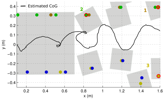
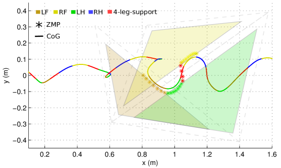
Figure 8: Top: The body motion when walking over the stepping stones is show in black. The planned footholds are shown and the irregular step sequence LF(1) $\rightarrow$ LH(2) $\rightarrow$ RF(3) is highlighted (red). Bottom: The 3 shrunk support triangles corresponding to the highlighted step sequence brown $\rightarrow$ green $\rightarrow$ yellow are shown. Additionally the planned CoG (solid line) and ZMP trajectory for the duration of these 3 steps is illustrated (asterix). While the CoG (solid line) does not reach the support triangles, the ZMP does, causing dynamic stability. When switching between disjoint support triangles (green $\rightarrow$ yellow) four-leg support phases are inserted (red) to allow a smooth transition.

VI-B5 Stability despite irregular swing-leg sequences

Walking over the stepping stones demonstrates the ability of the controller to execute irregular swing-leg sequences in a dynamically stable manner (Fig. 8). Starting from a lateral sequence gait (LH-LF-RH-RF) the foothold sequence changes to traverse these irregularly placed stepping stones. Despite this, the produced CoG trajectory (colored solid line) is dynamically stable, since the ZMP (asterisk) is always kept inside the current support triangle. When comparing the actual (top) and desired (bottom) CoG trajectories, a tracking error is evident. By keeping the ZMP e.g. d = 6 cm away from the stability borders, we are robust even against these inaccuracies.

The whole body motion generator inserts four-leg-support phases (red section) only whenever it detects disjoint support triangles in the swing-leg sequence. While executing steps 1 and 2 (Fig. 8) no four-leg-support phase is necessary, because the triangles are not disjoint. Only after returning to swing the right-front leg, the robot requires a four-leg support phase for the ZMP to transition from the green (LH) to the yellow (RF) support triangle at $(x,y)=(1.1,0)$.

VII Conclusion

We presented a dynamic, whole-body locomotion framework that executes footholds planned on-board. We showed, how a change in the environment causes the foothold generator to re-plan footholds on-line. We presented a whole body motion planner, which is able to generate a ZMP-stable body trajectory despite irregular swing-leg sequences to execute footholds dynamically. We showed how a combination of virtual model and floating-base inverse dynamics control can compliantly, yet accurately, track the desired whole-body motions. Real world experimental trials on challenging terrain demonstrate the capability of our framework.

We are currently working on bringing the kinematic planning and dynamic execution closer together. The idea is to produce desired state trajectories and required torques through one trajectory optimization problem, taking into account torque/joint limits, the dynamic model of the robot, foothold positions, friction coefficients and other constraints. With this approach we aim to produce even more dynamic motions such as jumping and rearing, during which fewer or no legs are in contact.

References

- [1] A. W. Winkler, I. Havoutis, S. Bazeille, J. Ortiz, M. Focchi, R. Dillmann, D. Caldwell, and C. Semini, “Path planning with force-based foothold adaptation and virtual model control for torque controlled quadruped robots,” in IEEE International Conference on Robotics and Automation (ICRA), 2014,
- [2] C. Semini, N. G. Tsagarakis, E. Guglielmino, M. Focchi, F. Cannella, and D. G. Caldwell, “Design of HyQ – a hydraulically and electrically actuated quadruped robot,” Journal of Systems and Control Engineering, 2011,
- [3] M. H. Raibert, Legged robots that balance. MIT press Cambridge, MA, 1986, vol. 3,
- [4] V. Barasuol, J. Buchli, C. Semini, M. Frigerio, E. R. De Pieri, and D. G. Caldwell, “A reactive controller framework for quadrupedal locomotion on challenging terrain,” in IEEE International Conference on Robotics and Automation (ICRA), 2013,
- [5] I. Havoutis, C. Semini, J. Buchli, and D. G. Caldwell, “Quadrupedal trotting with active compliance,” IEEE International Conference on Mechatronics (ICM), 2013,
- [6] M. Focchi, V. Barasuol, I. Havoutis, C. Semini, D. G. Caldwell, V. Barasul, and J. Buchli, “Local Reflex Generation for Obstacle Negotiation in Quadrupedal Locomotion,” International Conference on Climbing and Walking Robots and the Support Technologies for Mobile Machines (CLAWAR), pp. 1–8, 2013,
- [7] M. Kalakrishnan, J. Buchli, P. Pastor, M. Mistry, and S. Schaal, “Learning, planning, and control for quadruped locomotion over challenging terrain,” The International Journal of Robotics Research, vol. 30, no. 2, pp. 236–258, 2010,
- [8] J. R. Rebula, P. D. Neuhaus, B. V. Bonnlander, M. J. Johnson, and J. E. Pratt, “A controller for the littledog quadruped walking on rough terrain,” in IEEE International Conference on Robotics and Automation, 2007, pp. 1467–1473,
- [9] J. Z. Kolter, M. P. Rodgers, and A. Y. Ng, “A control architecture for quadruped locomotion over rough terrain,” in IEEE International Conference on Robotics and Automation (ICRA), 2008, pp. 811–818,
- [10] M. Zucker, N. Ratliff, M. Stolle, J. Chestnutt, J. A. Bagnell, C. G. Atkeson, and J. Kuffner, “Optimization and learning for rough terrain legged locomotion,” International Journal of Robotics Research (IJRR), vol. 30, no. 2, pp. 175–191, Feb. 2011,
- [11] S. Kajita, F. Kanehiro, K. Kaneko, K. Fujiwara, K. Harada, K. Yokoi, and H. Hirukawa, “Biped walking pattern generation by using preview control of zero-moment point,” 2003 IEEE International Conference on Robotics and Automation, pp. 1620–1626, 2003,
- [12] C. Mastalli, I. Havoutis, A. W. Winkler, D. G. Caldwell, and C. Semini, “On-line and on-board planning for quadrupedal locomotion, using practical, on-board perception,” in IEEE International Conference on Technologies for Practical Robot Applications (TePRA), May 2015,
- [13] A. Hornung, K. M. Wurm, M. Bennewitz, C. Stachniss, and W. Burgard, “OctoMap: An efficient probabilistic 3D mapping framework based on octrees,” Autonomous Robots, 2013,
- [14] M. Bloesch, M. Hutter, M. Hoepflinger, S. Leutenegger, C. Gehring, C. Remy, and R. Siegwart, “State estimation for legged robots - consistent fusion of leg kinematics and imu,” in Robotics: Science and Systems Conference (RSS), 2012,
- [15] M. Likhachev, G. J. Gordon, and S. Thrun, “Ara*: Anytime a* with provable bounds on sub-optimality,” in Advances in Neural Information Processing Systems, 2003, p. None,
- [16] G. Guennebaud, A. Furfaro, and L. D. Gaspero, “eiquadprog.hh,” 2011,”
- [17] J. Pratt, C.-M. Chew, A. Torres, P. Dilworth, and G. Pratt, “Virtual model control: An intuitive approach for bipedal locomotion,” International Journal of Robotics Research (IJRR), 2001,
- [18] F. Caccavale, C. Natale, B. Siciliano, and L. Villani, “Six-DOF impedance control based on angle/axis representations,” IEEE Transactions on Robotics and Automation, vol. 15, pp. 289–300, 1999,
- [19] Y. Fujimoto, S. Obata, and A. Kawamura, “Robust biped walking with active interaction control between foot and ground,” Proceedings. 1998 IEEE International Conference on Robotics and Automation (Cat. No.98CH36146), vol. 3, 1998,
- [20] R. Featherstone, Rigid Body Dynamics Algorithms. Boston, MA: Springer US, 2008.