On-line and On-board Planning and Perception for Quadrupedal Locomotion

Abstract

We present a legged motion planning approach for quadrupedal locomotion over challenging terrain. We decompose the problem into body action planning and footstep planning. We use a lattice representation together with a set of defined body movement primitives for computing a body action plan. The lattice representation allows us to plan versatile movements that ensure feasibility for every possible plan. To this end, we propose a set of rules that define the footstep search regions and footstep sequence given a body action. We use Anytime Repairing A* (ARA*) search that guarantees bounded sub-optimal plans. Our main contribution is a planning approach that generates on-line versatile movements. Experimental trials demonstrate the performance of our planning approach in a set of challenging terrain conditions. The terrain information and plans are computed on-line and on-board.

I Introduction

Legged motion planning over rough terrain involves making careful decisions about the footstep sequence, body movements, and locomotion behaviors. Moreover, it should consider whole-body dynamics, locomotion stability, kinematic and dynamic capabilities of the robot, mechanical properties and irregularities of the terrain. Frequently, locomotion over rough terrain is decomposed into: (a) perception and planning to reason about terrain conditions, by computing a plan that allows the legged system to traverse the terrain toward a goal, and (b) control that executes the plan while compensating for uncertainties in perception, modelling errors, etc. In this work, we focus on generating on-line and versatile plans for quadruped locomotion over challenging terrain.

In legged motion planning one can compute simultaneously contacts and body movements, leading to a coupled motion planning approach [1][2][3][4]. This can be posed as a hybrid system or a mode-invariant problem. Such approaches tend to compute richer motion plans than decoupled motion planners, especially when employing mode-invariant strategies. Nevertheless, these approaches are often hard to use in a practical setting. They are usually posed as non-linear optimization problems such as Mathematical Programming with Complementary Constraints [3], and are computationally expensive. On the other hand, the legged motion planning problem can be posed as a decoupled approach that is naturally divided into: motion and contact planning [5][6][7]. These approaches avoid the combinatorial search space at the expense of complexity of locomotion. A decoupled motion planner has to explore different plans in the space of feasible movements (state space), which is often defined by physical, stability, dynamic and task constraints. Nevertheless, the feasibility space is variable since the stability constraints depend on the kind of movement, e.g. static or dynamic walking.

The challenge of decoupled planners lies primarily in reducing the computation time while increasing the complexity of motion generation. To the best of our knowledge, up to now, decoupled approaches are limited in the versatility of movements and computation time, for instance [5] reduces the computation time but is still limited to small changes of the robot’s yaw (heading). Therefore, our main contribution is a planning approach that increases the versatility of plans, based on the definition of footstep search regions and footstep sequence according to a body action plan. Our method computes on-line and on-board plans (around 1 Hz) using the incoming perception information on commodity hardware. We evaluate our planning approach on the Hydraulic Quadruped robot -HyQ- [8] shown in Fig. 1.

The rest of the paper is structured as follows: after discussing previous research in the field of legged motion planning (Section II). Section III explains, how on-line and on-board versatile plans are generated based on a decoupled planning approach (body action and footstep sequence planners). In Section IV we evaluate the performance of our planning approach in real-world trials before Section V summarizes this work and presents ideas for future work.

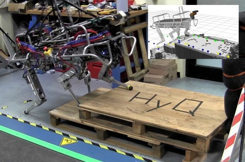
Figure 1: The hydraulically actuated and fully torque-controlled quadruped robot HyQ [8]. The inset plot shows the on-line environment perception alongside with the planned footholds and the current on-board robot state estimate.

II Related Work

Motion planning is an important problem for successful legged locomotion in challenging environments. Legged systems can utilize a variety of dynamic gaits (e.g. trotting and galloping) in environments with smooth and continuous support such as flats, fields, roads, etc. Such cyclic gaits often assume that contact will be available within the reachable workspace at every step. However, for more complex environments, reactive cyclic gait generation approaches quickly reach their capabilities as foot placement becomes crucial for the success of the behavior.

Natural locomotion over rough terrain requires simultaneous computation of footstep sequences, body movements and locomotion behaviors (coupled planning) [1][2][3][4]. One of the main problems with such approaches is that the search space quickly grows and searching becomes unfeasible, especially for systems that require on-line solutions. In contrast, we can state the planning and control problem into a set of sub-problems, following a decoupled planning strategy. For example the body path and the footstep planners can be separated, thus reducing the search space for each component [5][6][7]. This can reduce the computation time at the expense of limiting the planning capabilities, sometimes required for extreme rough terrain. There are two main approaches of decoupled planning: contact-before-motion [9][10][6] and motion-before-contact [11][5]. These approaches find a solution in motion space, which defines the possible motion of the robot.

The motion space of contact-before-motion planner lies in a sub-manifold of the configuration space with certain motion constraints, thus, a footstep constraint switches the motion space to a lower-dimensional sub-manifold $Q_{\sigma}$ [12][13]. Therefore, these planners have to find a path that connects the initial $F_{\sigma}$ and goal $F_{\sigma^{\prime}}$ feasible regions. Note that the planner must find transitions between feasible regions and then compute paths between all the possible stances (feasible regions) that connect $F_{\sigma}$ and $F_{\sigma^{\prime}}$, which is often computationally expensive. On the other hand, motion-before-contact approaches allow us to shrink the search space using an intrinsic hierarchical decomposition of the problem into; high-level planning, body-path planning and footstep planning, and low-level planning, CoG trajectory and foot trajectory generation. These approaches reduce considerably the search space but can also limit the complexity of possible movements, nevertheless [5], [14] and [15] have demonstrated that this can be a successful approach for rough terrain locomotion. Nonetheless these approaches were tailored for specific types of trials where goal states are mostly placed in front of the robot. This way most of these frameworks developed planners that use a fixed yaw and only allow forward expansion of the planned paths. Our approach takes a step forward in versatility by allowing motion in all directions and changes in the robot’s yaw (heading) as in real environments this is almost always required.

The planning approach described in this paper decouples the problem into: body action and footstep sequence planning (motion-before-contact). The decoupling strategy allows us to reduce the computation time, ensures sub-optimal plans, and computes plans on-line using the incoming information of the terrain. Our body action planner uses a lattice representation based on body movement primitives. Compared to previous approaches our planning approach generates on-line more versatile movements (i.e. forward and backward, diagonal, lateral and yaw-changing body movements) while also ensure feasibility for every body action. Both planning and perception are computed on-line and on-board.

III Technical Approach

Our overall task is to plan on-line an appropriate sequence of footholds $\mathbf{F}$ that allows a quadruped robot to traverse a challenging terrain toward a body goal state $(x,y,\theta)$. To accomplish this, we decouple the planning problem into: body action and footstep sequence planning. The body action planner searches a bounded sub-optimal solution around a growing body-state graph. Then, the footstep sequence planner selects a foothold sequence around an action-specific foothold region of each planned body action.

Clearly, decoupled approaches reduce the combinatorial search space at the expense of the complexity of locomotion. This limits the versatility of the body movement (e.g. discretized yaw–changing movements instead of continuous changes). Nevertheless, our approach manages this trade-off by employing a lattice representation of potentially feasible body movements and action-specific foothold regions.

III-A Terrain Reward Map

The terrain reward map quantifies how desirable it is to place a foot at a specific location. The reward value for each cell in the map is computed using geometric terrain features as in [15]. Namely we use the standard deviation of height values, the slope and the curvature as computed through regression in a 6cm$\times$6cm window around the cell in question; the feature are computed from a voxel model (2 cm resolution) of the terrain. We incrementally compute the reward map based on the aforementioned features and recompute locally whenever a change in the map is detected. For this we define an area of interest around the robot of 2.5m$\times$5.5m that uses a cell grid resolution of 4 cm. The cost value for each cell of the map is computed as a weighted linear combination of the individual feature $R(x,y)=\mathbf{w}^{T}\mathbf{r}(x,y)$, where $\mathbf{w}$ and $\mathbf{r}(x,y)$ are the the weights and features values, respectively. Figure 2 shows the generation of the reward map from the mounted RGBD sensor. The reward values are represented using a color scale, where blue is the maximum reward and red is the minimum one.

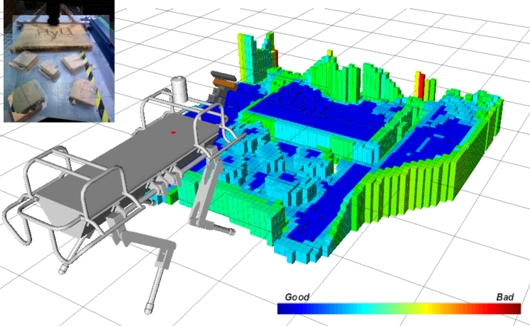
Figure 2: The reward map generation from RGBD (Asus Xtion) camera data. The RBGD sensor is mounted on a PTU unit that scans the terrain. An occupancy map is built with a 2 cm resolution. Then the set of features is computed and the total reward value per pixel of 4 cm is calculated. In addition, a height map of 2 cm resolution in $z$ is created. The reward values are represented using a color scale, where blue is the maximum reward and red is the minimum one.

III-B Body Action Planning

A body action plan over challenging terrain take into consideration the wide range of difficulties of the terrain, obstacles, type of action, potential shin collisions, potential body orientations and kinematic reachability. Thus, given a reward map of the terrain, the body action planner computes a sequence of body actions that maximize the cross-ability of the sub-space of candidate footsteps. The body action plans are computed by searching over a body-state graph that is built using a set of predefined body movements primitives. The body action planning is described in Algorithm 1.

Data: Inflation parameter $\epsilon$, time of computation $t_{c}$

Result: a body action plan $\mathbf{Q}=[\mathbf{q}^{0},\mathbf{q}^{1},\cdots,\mathbf{q}^{l}]$

function computeBodyActionPlan($\mathbf{s}_{start},\mathbf{s}_{goal}$)

     set $\epsilon$ and computation time $t_{c}$

     $g(\mathbf{s}_{start})=0;g(\mathbf{s}_{goal})=\infty$

     OPEN $=\{\mathbf{s}_{start}\}$; INCONS $=$ CLOSED$=\emptyset$

     while ($\epsilon\geq 1$ and $t_{c}<t$) do

         decrease $\epsilon$

         OPEN $=$ OPEN $\cup$ INCONS; CLOSED $=\emptyset$

         // fval$(\mathbf{s})=g(\mathbf{s})+\epsilon h(\mathbf{s})$

         while (fval$(\mathbf{s}_{goal})>$ minimum fval in OPEN) do

              remove $\mathbf{s}$ with minimum fval from OPEN

              insert $\mathbf{s}$ into CLOSED

              generate action($\mathbf{s}$) from body primitives

              for all $\mathbf{u}\in$ action($\mathbf{s}$) do

                  compute $\mathbf{s^{\prime}}$ given $\mathbf{u}$

                  compute the footstep regions given $\mathbf{s^{\prime}}$

                  compute $c_{body}(\mathbf{s},\mathbf{s^{\prime}})$ from footstep regions

                  if $g(\mathbf{s^{\prime}})>g(\mathbf{s})+c_{body}(\mathbf{s},\mathbf{s^{\prime}})$ then

                       $g(\mathbf{s^{\prime}})=g(\mathbf{s})+c_{body}(\mathbf{s},\mathbf{s^{\prime}})$

                       add $\mathbf{s}\mapsto\mathbf{s^{\prime}}$ to policy $\mathbf{s^{\prime}}=\pi(\mathbf{s})$

                       if $\mathbf{s^{\prime}}$ is not in CLOSED then

                           insert ($\mathbf{s^{\prime}},$fval($\mathbf{s^{\prime}}$)) into OPEN

                       else

                           insert ($\mathbf{s^{\prime}}$, fval($\mathbf{s^{\prime}}$)) into INCONS

                       end if

                  end if

              end for

         end while

     end while

     reconstruct body action plan $\mathbf{Q}$ from $\pi(\cdot)$

     return $\mathbf{Q}$

end function

Algorithm 1 Computes a set of body action over a challenging terrain using an ARA^∗ search.

III-B1 Graph construction

We construct the body-state graph using a lattice-based adjacency model. Our lattice representation is a discretization of the configuration space into a set of feasible body movements, in which the feasibility depends on the selected sequence of footholds around the movement. The body-state graph represents the transition between different body-states (nodes) and it is defined as a tuple, $\mathcal{G}=(\mathcal{S},\mathcal{E})$, where each node $\mathbf{s}\in\mathcal{S}$ represents a body-state and each edge $\mathbf{e}\in\mathcal{E}\subseteq\mathcal{S}\times\mathcal{S}$ defines a potential feasible transition from $\mathbf{s}$ to $\mathbf{s^{\prime}}$. A sequence of body-states (or body poses $(x,y,\theta)$) approximates the body trajectory that the controller will execute. An edge defines a feasible transition (body action) according to a set of body movement primitives. The body movement primitives are defined as body displacements (or body actions), which ensure feasibility together with a feasible footstep region. A feasible footstep region is defined according to the body action.

Given a body-state query, a set of successor states are computed using a set of predefined body movement primitives. A predefined body movement primitive connects the current body state $\mathbf{s}=(x,y,\theta)$ with the successor body state $\mathbf{s^{\prime}}=(x^{\prime},y^{\prime},\theta^{\prime})$. The graph $\mathcal{G}$ is dynamically constructed due to the associated cost of transition $c_{body}(\mathbf{s},\mathbf{s^{\prime}})$ depends on the current and next states (or current state and action). In fact, the feasible regions of foothold change according to each body action, which affect the value of the transition cost. Moreover, an entire graph construction could require a greater memory pre-allocation and computation time than available (on-board computation). Figure 3 shows the graph construction for the body action planner. The associated cost of every transition $c_{body}(\mathbf{s},\mathbf{s^{\prime}})$ is computed using the footstep regions. These footstep regions depend on the body action in such a way that they ensure feasibility of the plan, as is explained in III-B4 subsection. For every expansion, the footstep regions of Left-Front LF (brown squares), Right-Front RF (yellow squares), Left-Hind LH (green squares) and Right-Hind RH (blue squares) legs are computed given a body action.

The resulting states $\mathbf{s^{\prime}}$ are checked for body collision with obstacles, using a predefined area of the robot, and invalid states are discarded. For legged locomotion over challenging terrain, obstacles are defined as unfeasible regions to cross, e.g. a wall or tree. In our case, the obstacles are detected when the height deviation w.r.t. the estimated plane of the ground is larger than the kinematic feasibility of the system in question (HyQ). We build the obstacle map with 8 cm resolution, otherwise it would be computationally expensive due to the fact that it would increase the number of collision checks. In fact, the body collision checker evaluates if there are body cells in the resulting state that collide with an obstacle.

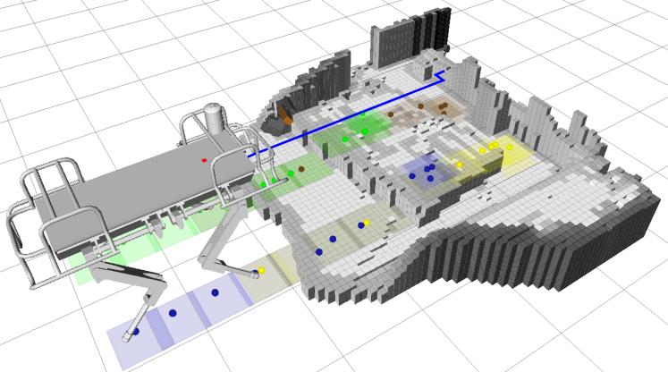
Figure 3: Illustration of graph construction of the least-cost path. The associated cost of every transition $c_{body}(\mathbf{s},\mathbf{s^{\prime}})$ is computed using the footstep regions. For every expansion, the footstep regions of LF (brown squares), RF (yellow squares), LH (green squares) and RH (blue squares) are computed according to a certain body action.

III-B2 Body cost

The body cost describes how desirable it is to cross the terrain with a certain body path (or body actions). This cost function is designed to maximize the cross-ability of the terrain while minimizing the path length. In fact, the body cost function $c_{body}$ is a linear combination of: terrain cost $c_{t}$, action cost $c_{a}$, potential shin collision cost $c_{pc}$, and potential body orientation cost $c_{po}$. The cost of traversing any transition between the body state $\mathbf{s}$ and $\mathbf{s^{\prime}}$ is defined as follows:

$$c_{body}(\mathbf{s},\mathbf{s^{\prime}})=w^{b}_{t}c_{t}(\mathbf{s})+w_{a}c_{a}(\mathbf{s},\mathbf{s^{\prime}})$$

$$+w_{pc}c_{pc}(\mathbf{s})+w_{po}c_{po}(\mathbf{s})$$ (1)

where $w_{i}$ are the respective weight of the different costs.

For a given current body state $(x,y,\theta)$, the terrain cost $c_{t}$ is evaluated by averaging the best $n$-footsteps terrain reward values around the foothold regions of a nominal stance (nominal foothold positions). The action cost $c_{a}$ is defined by the user according to the desirable actions of the robot, e.g. it is preferable to make diagonal body movements than lateral ones. The potential leg collision cost $c_{pc}$ is computed by searching potential obstacles in the predefined workspace region of the foothold, e.g. near to the shin of the robot. In fact, a potential shin collision is detected around a predefined shin collision region, which depends on the configuration of each leg as shown in Figure 4. This cost is proportional to the height defined around the footstep plane, where red bars represent collision elements. Finally, the potential body orientation $c_{po}$ is estimated by fitting a plane in the possible footsteps around the nominal stance for each leg.

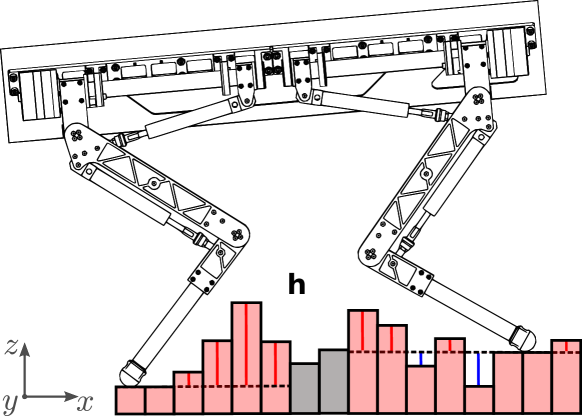
Figure 4: Computation of the potential shin collision. The potential shin collisions are detected around a predefined shin collision region (red bars). The computed cost is proportional to the height defined (red lines) around the footstep plane (dashed black lines), where blue height differences do not contribute to the cost.

III-B3 Reducing the search space

Decoupling the planning problem into body action and footstep planning avoids the combinatorial search space. This allows us to compute plans on-line, and moreover, to develop a closed-loop planning approach that can deal with changes in the environment. Nevertheless the reduced motion space might span infeasible regions due to the strong coupling between the body action and footstep plans. A strong coupling makes that a feasible movement depends on the whole plan (body action and footstep sequence). In contrast to previous approaches [5][6][14][11][15], our planner uses a lattice-based representation of the configuration space. The lattice representation uses a set of predefined body movement primitives that allows us to apply a set of rules that ensure feasibility in the generation of on-line plans.

The body movement primitives are defined as 3D motion-actions $(x,y,\theta)$ of the body that discretize the search space. We implement a set of different movements (body movement primitives) such as: forward and backward, diagonal, lateral and yaw-changing movements.

III-B4 Ensuring feasibility

Our lattice representation allows the robot to search a body action plan according to a set of predefined body movement primitives. A predefined body movement primitive cannot guarantee a feasible plan due to the mutual dependency of movements and footsteps. For instance, the feasibility of clockwise movements depends on the selected sequence of footsteps, and can only be guaranteed in a specific footstep region. In fact, we exploit this characteristic in order to ensure feasibility in each body movement primitive. These footstep regions increase the support triangle areas given a certain body action, improving the execution of the whole-body plan. This strategy also guarantees that the body trajectory generator can connect the support triangles (support triangle switching) [14]. Figure 5 illustrates the footstep regions according to the type of body movement primitives. These footstep regions are tuned to increase the triangular support areas, improving the execution of the whole-body plan.

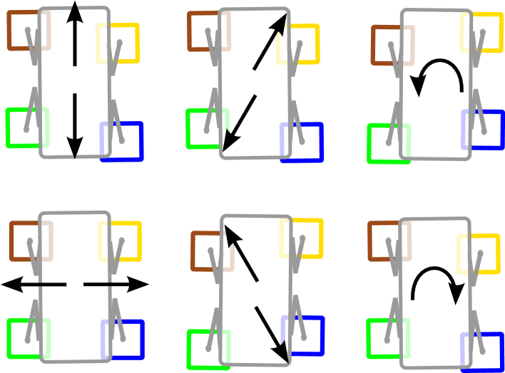
Figure 5: Different footstep search regions according to the body action. These footstep regions ensure the feasibility of the plan. Moreover, it increase the triangular support areas, improving the execution of the whole-body plan. The brown, yellow, green and blue squares represent the footstep search regions for LF, RF, LH and RH feet, respectively.

III-B5 Heuristic function

The heuristic function guides the search to promising solutions, improving the efficiency of the search. Heuristic-based search algorithms require that the heuristic function is admissibile and consistent. Most of the heuristic functions estimate the cost-to-go by computing the Euclidean distance to the goal. However, these kind of heuristic functions do not consider the terrain conditions. Therefore, we implemented a terrain-aware heuristic function that considers the terrain conditions.

The terrain-aware heuristic function computes the estimated cost-to-go by averaging the terrain cost locally and estimating the number of footsteps to the goal:

$$h(\mathbf{s})=-\bar{R}\mathcal{F}(\|\mathbf{g}-\mathbf{s}\|)$$ (2)

where $\bar{R}$ is the average reward (or cost) and $\mathcal{F}(\|\mathbf{g}-\mathbf{s}\|)$ is the function that estimates the number of footsteps to the goal.

III-B6 Ensuring on-line planning

Open-loop planning approaches fail to deal adequately with changes in the environment. In real scenarios, the robot has a limited range of perception that makes open-loop planning approaches unreliable. Closed-loop planning considers the changes in the terrain conditions, and uses predictive terrain conditions for non-perceived regions, improving the robustness of the plan. Dealing with re-planning and updating of the environment information requires that the information is managed in an efficient search exploration of the state space. We manage to reduce the computation time of building a reward map by computing the reward values from a voxelized map of the environment. Additionally, we (re-)plan and update the information using ARA^∗ [16]. ARA^∗ ensures provable bounds on sub-optimality, depending on the definition of the heuristic function. On the other hand, the terrain-aware heuristic function guides the search according to terrain conditions.

III-C Footstep Sequence Planning

Given the desirable body action plan, $\mathbf{Q}=(\mathbf{x}_{d},\mathbf{y}_{d},\boldsymbol{\theta}_{d})$, the footstep sequence planner computes the sequence of footholds that reflects the intention of the body action. A local greedy search procedure selects the optimal footstep target. A (locally optimal) footstep is selected from defined footstep search regions by the body action planner. For every body action, the footstep planner finds a sequence of the 4-next footsteps. The footstep sequence planning is described in Algorithm 2.

Data: footstep horizon F

Result: a footstep sequence F

function computeFootstepSequence($\mathbf{Q}$)

     set horizon F

     for $\mathbf{q}_{i=0:F}\in\mathbf{Q}$ do

         for i=0:3 do

              compute the sequence of footstep $e$ given $\mathbf{q}_{i}$

              generate possible FOOTSTEP($e,\mathbf{q}_{i}$)

              compute the greedy solution $\mathbf{f}_{min}$

              add $\mathbf{f}_{min}$ to $\mathbf{F}$

         end for

     end for

     return $\mathbf{F}$

end function

Algorithm 2 Computes a footstep sequence given a body action plan.

III-C1 Footstep cost

The footstep cost describes how desirable is a foothold target, given a body state $\mathbf{s}$. The purpose of this cost function is to maximize the locomotion stability given a candidate set of footsteps. The footstep cost $c_{footstep}$ is a linear combination of: terrain cost $c_{t}$, support triangle cost $c_{st}$, shin collision cost $c_{c}$ and body orientation cost $c_{o}$. The cost of certain footstep $\mathbf{f}^{e}$ is defined as follows:

$$c_{footstep}(\mathbf{f}^{e})=w^{f}_{t}c_{t}(\mathbf{f}^{e})+w_{st}c_{st}(\mathbf{f}^{e})$$

$$+w_{c}c_{c}(\mathbf{f}^{e})+w_{o}c_{o}(\mathbf{f}^{e})$$ (3)

where $\mathbf{f}^{e}$ defines the Cartesian position of the foothold target $e$ (foot index). We consider as end-effectors: the LF, RF, LH and RH feet of HyQ.

The terrain cost $c_{t}$ is computed from the terrain reward value of the candidate foothold, i.e. using the terrain reward map (see Figure 2). The support triangle cost $c_{st}$ depends on the inradii of the triangle formed by the current footholds and the candidate one. As in the body cost computation, we use the same predefined collision region around the candidate foothold. Finally, the body orientation cost $c_{o}$ is computed using the plane formed by the current footsteps and the candidate one. We calculate the orientation of the robot from this plane.

IV Experimental Results

The following section describes the experiments conducted to validate the effectiveness and quantify the performance of our planning approach.

IV-A Experimental Setup

We implemented and tested our approach with HyQ, a Hydraulically actuated Quadruped robot developed by the Dynamic Legged Systems (DLS) Lab [8]. HyQ roughly has the dimensions of a medium-sized dog, weight 90 kg, is fully-torque controlled and is equipped with precision joint encoders, a depth camera (Asus Xtion) and an Inertial Measurement Unit (IMU). We used an external state measuring system, Vicon marker-based tracker system. The perception and planning is done on-board in an i7/2.8GHz PC, and all computations of the real-time controller are done using a PC104 stack.

The first set of experiments are designed to test the capabilities of our motion planner. We use a set of benchmarks of realistic locomotion scenarios (see Figure 6): stepping stones, pallet, stair and gap. In these experiments, we compared the cost, number of expansions and computation time of ARA^∗ against A^∗ [16] using our lattice representation. The results are based on 9 predefined goal locations. Second experiment, the robot must plan on-line with dynamic changes in the terrain. Third experiment, the next experiment we show the on-line planning and perception results. Finally, we validate the performance of our planning approach by executing in HyQ.

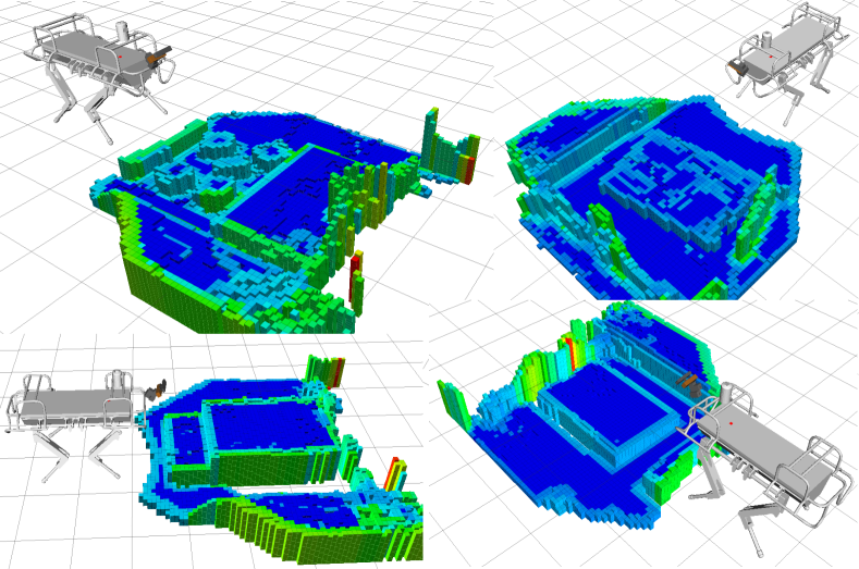
Figure 6: The planning benchmarks used to analyse the quality of the produced plans. Top left: stepping stones; top right: pallet; bottom left: stair; bottom right: gap.

IV-B Results and Discussions

IV-B1 Initial plan results

The stepping stones, pallet, stair and gap experiments (see Figure 6) show the initial plan quality (see Table I) of our approach using A^∗ and ARA^∗. To this end, we plan a set of body actions and footstep sequences for 9 predefined goal locations, approximately 2.0 m away from the starting position, and compare the cost and number of expansions of the body action path, and the planning time of ARA^∗ against A^∗. Three main factors contribute to the decreased planning time while maintaining the quality of the plan:

First, the lattice-based representation (using body movement primitives) considers versatile movements in the sense that it allows us to reduce the search space around feasible regions (feasible motions) according a certain body action, in contrast to grid-based approaches that ensure the feasibility by applying rules that are agnostic to body actions. Second, our terrain-aware heuristic function guides the tree expansion according to terrain conditions in contrast to a simple Euclidean heuristic. Finally, the ARA* algorithm implements a search procedure that guarantees bounded sub-optimality in the solution given a proper heuristic function [16]. Figure 7 shows the initial plan of A* and ARA*.

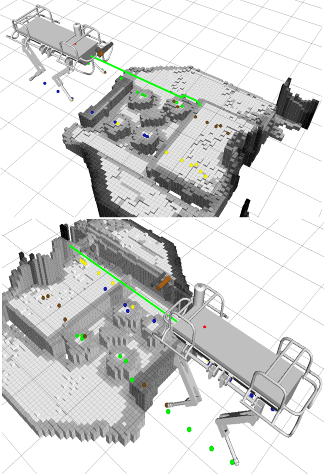
Figure 7: Comparison of the body action (green line) and footstep sequence computed plan A^∗ and ARA* given reward map (grey scale). The brown, yellow, green and blue points represent the planned footsteps of the LF, RF, LH and RH feet, respectively. The top image shows the computed plan by A^∗, and the bottom one the results of ARA^∗.

TABLE I: Cost of the plan (Cost), number of expansions (Exp.) and computation time (Time) averaged over 9 trials of A^∗ and ARA^∗.

	A*			ARA*
Terrain	Cost	Exp.	Time [s]	Cost	Exp.	Time [s]
S. Stones	364.7	3191	428.7	597.4	12.1	1.59
Pallet	269.2	270	271.2	587.7	12.7	1.74
Stair	306.1	306	308.1	646.4	12.7	1.55
Gap	325.6	326	327.6	647.0	13.0	2.01

IV-B2 On-line planning and perception

Using a movement primitive-based lattice search reduces the size of the search space significantly, leading to responsive planning and replanning. In our experimental trials, we choose a lattice graph resolution (discretization) of 4 cm for $x/y$ and 1.8^∘ for $\theta$ and goal state is never more that 5 m away from the robot. In these trials, the plan/replan frequency is approximately 0.5 Hz.

The efficient occupancy grid-based mapping allows us to incrementally build up the model of the environment and focus our computations to the area of interest around the robot body, generating plans quickly. This allows us to locally update the computed reward map and incrementally build the reward map as the robot moves with an average response frequency of 2 Hz as is shown in Figure 9.

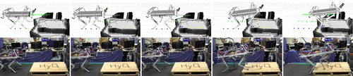
Figure 8: Snapshots of pallet trial used to evaluate the performance of our planning approach. From top to bottom: planning and terrain reward map; execution of the plan with HyQ.

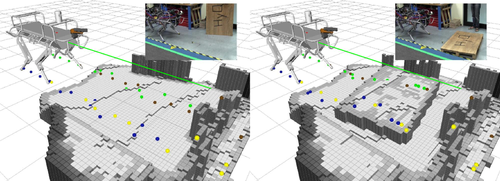
Figure 9: (Re-)planning and perception on-board. The left image presents the plan for a flat terrain, then, the right image reflects the re-planning and updating of the reward map (grey scale map). The green, brown, blue and yellow points represent the planned footholds of the LH, LF, RH, RF legs, respectively. The green line represents the body path according to action plan.

IV-B3 Planning and execution

We generate swift and natural dynamic whole-body motions from an n-step lookahead optimization of the body trajectory that uses a dynamic stability metric, the Zero Moment Point (ZMP). A combination of floating-base inverse dynamics and virtual model control accurately executes such dynamic whole-body motions with an actively compliant system [17]. Figure 8 shows the execution of an initial plan. Our locomotion system is robust due to a combination of on-line planning and compliance control.

V Conclusion

We presented a planning approach that allows us to plan on-line, versatile movements. Our approach plans a sequence of footsteps given a body action plan. The body action planner guarantees a bounded sub-optimal plan given a set of predefined body movement primitives (lattice representation). In general, to generate versatile movement one has to explore a considerable region of the motion space, making on-line planning a computationally challenging task, especially in practical applications. Here, we reduce the exploration by ensuring the feasibility of every possible body action. In fact, we define the footstep search regions and footstep sequence based on the body action. We showed how our planning approach computes on-line plans given incoming terrain information. Various real-world experimental trials demonstrate the capability of our planning approach to traverse challenging terrain.

References

- [1] Y. Tassa and E. Todorov, “Stochastic Complementarity for Local Control of Discontinuous Dynamics,” in Proceedings of Robotics: Science and Systems, 2010,
- [2] I. Mordatch, E. Todorov, and Z. Popović, “Discovery of complex behaviors through contact-invariant optimization,” ACM Transactions on Graphics, vol. 31, no. 4, pp. 1–8, July 2012,
- [3] M. Posa, C. Cantu, and R. Tedrake, “A direct method for trajectory optimization of rigid bodies through contact,” The International Journal of Robotics Research, Oct. 2013,
- [4] H. Dai, A. Valenzuela, and R. Tedrake, “Whole-body motion planning with simple dynamics and full kinematics,” in 14th IEEE-RAS International Conference on Humanoid Robots, 2014,
- [5] J. Z. Kolter, M. P. Rodgers, and A. Y. Ng, “A control architecture for quadruped locomotion over rough terrain,” in IEEE International Conference on Robotics and Automation (ICRA), 2008, pp. 811–818,
- [6] P. Vernaza, M. Likhachev, S. Bhattacharya, A. Kushleyev, and D. D. Lee, “Search-based planning for a legged robot over rough terrain,” in IEEE International Conference on Robotics and Automation, 2009,
- [7] M. Kalakrishnan, J. Buchli, P. Pastor, and S. Schaal, “Learning locomotion over rough terrain using terrain templates,” in IEEE/RSJ International Conference on Intelligent Robots and Systems (IROS), 2009, pp. 167–172,
- [8] C. Semini, N. G. Tsagarakis, E. Guglielmino, M. Focchi, F. Cannella, and D. G. Caldwell, “Design of HyQ – a hydraulically and electrically actuated quadruped robot,” Proceedings of the Institution of Mechanical Engineers, Part I: Journal of Systems and Control Engineering, 2011,
- [9] A. Escande, A. Kheddar, and S. Miossec, “Planning support contact-points for humanoid robots and experiments on HRP-2,” in IEEE/RSJ International Conference on Intelligent Robots and Systems. IEEE, Oct. 2006, pp. 2974–2979,
- [10] K. Hauser and J. C. Latombe, “Multi-modal Motion Planning in Non-expansive Spaces,” The International Journal of Robotics Research, vol. 29, no. 7, pp. 897–915, Oct. 2009,
- [11] M. Zucker, J. A. Bagnell, C. Atkeson, and J. Kuffner, “An Optimization Approach to Rough Terrain Locomotion,” in IEEE International Conference on Automation and Robotics ICRA, 2010,
- [12] K. Hauser and V. Ng-Thow-Hing, “Randomized multi-modal motion planning for a humanoid robot manipulation task,” The International Journal of Robotics Research, vol. 30, no. 6, pp. 678–698, Dec. 2010,
- [13] A. Escande, A. Kheddar, and S. Miossec, “Planning contact points for humanoid robots,” Robotics and Autonomous Systems, vol. 61, no. 5, pp. 428–442, May 2013,
- [14] M. Kalakrishnan, J. Buchli, P. Pastor, M. Mistry, and S. Schaal, “Learning, planning, and control for quadruped locomotion over challenging terrain,” The International Journal of Robotics Research, vol. 30, no. 2, pp. 236–258, 11 2010,
- [15] A. W. Winkler, I. Havoutis, S. Bazeille, J. Ortiz, M. Focchi, D. Caldwell, and C. Semini, “Path planning with force-based foothold adaptation and virtual model control for torque controlled quadruped robots,” in IEEE International Conference on Robotics and Automation (ICRA), 2014,
- [16] M. Likhachev, G. Gordon, and S. Thrun, “ARA*: Anytime A* with Provable Bounds on Sub-Optimality,” in Advances in Neural Information Processing Systems 16: Proceedings of the 2003 Conference (NIPS-03). MIT Press, 2004.
- [17] A. W. Winkler, C. Mastalli, I. Havoutis, M. Focchi, D. Caldwell, and C. Semini, “Planning and Execution of Dynamic Whole-Body Locomotion for a Hydraulic Quadruped on Challenging Terrain,” in IEEE International Conference on Robotics and Automation (ICRA), 2015,