Precise prediction for the W boson mass in the MRSSM

Abstract

The mass of the W boson, $\MW$, plays a central role for high-precision tests of the electroweak theory. Confronting precise theoretical predictions with the accurately measured experimental value provides a high sensitivity to quantum effects of the theory entering via loop contributions. The currently most accurate prediction for the W boson mass in the Minimal R-symmetric Supersymmetric Standard Model (MRSSM) is presented. Employing the on-shell scheme, it combines all numerically relevant contributions that are known in the Standard Model (SM) in a consistent way with all MRSSM one-loop corrections. Special care is taken in the treatment of the triplet scalar vacuum expectation value $v_{T}$ that enters the prediction for $\MW$ already at lowest order. In the numerical analysis the decoupling properties of the supersymmetric loop contributions and the comparison with the MSSM are investigated. Potentially large numerical effects of the MRSSM-specific $\Lambda$ superpotential couplings are highlighted. The comparison with existing results in the literature is discussed.

1 Introduction

Supersymmetry (SUSY) is seen as one of the most attractive extensions of the Standard Model (SM) of particle physics. It provides a solution for the hierarchy problem of the SM and a prediction for the mass of the scalar resonance discovered at the LHC ATLAS:2012gk ; Chatrchyan:2012ufa ; Aad:2015zhl if it is appropriately identified with one of the neutral Higgs bosons of the considered supersymmetric model.

So far, no further new state has been discovered at the LHC. The search limits from the LHC and previous colliders give rise to strong constraints on the parameter space of the Minimal Supersymmetric Standard Model (MSSM). The impact of those search limits may be much smaller for models with extended SUSY sectors. In particular, the introduction of R-symmetry Kribs:2012gx leads to models where the limits on the particle masses are significantly weaker and where accordingly the discovery of TeV-scale SUSY is still in reach of current experiments.

The LHC phenomenology of the Minimal R-symmetric Supersymmetric Standard Model (MRSSM) Kribs:2007ac and other models with R-symmetry has recently been explored in refs. PD1 ; PD2 ; PD3 ; PD4 ; Kotlarski:2016zhv ; Beauchesne:2017jou ; Benakli:2018vqz ; Alvarado:2018rfl ; Darme:2018dvz ; Chalons:2018gez . The signatures of the MRSSM differ from the ones of the MSSM as the model includes Dirac gauginos and higgsinos instead of Majorana ones. This goes hand in hand with additional states in the Higgs sector including an SU$(2)$ triplet, which may acquire a vacuum expectation value breaking the custodial symmetry of the electroweak sector. Additionally, R-symmetry forbids all soft SUSY-breaking trilinear couplings between Higgs bosons and squarks or sleptons, which removes unwanted sources of flavour violation which exist in the MSSM.

Even with no direct signals of SUSY indirect probes like electroweak precision observables can provide sensitivity to SUSY contributions above the direct experimental reach. Here we study the prediction for the mass of the W gauge-boson, $M_{W}$. The world average combining LEP and Tevatron results Schael:2013ita ; Aaltonen:2013iut is

$$M_{W}^{\text{exp.}}=80.385\pm 0.015\text{ GeV}\;.$$ (1)

It may be improved by measurements of the LHC experiments, where a first ATLAS result at $\sqrt{s}=7$ TeV reports a value Aaboud:2017svj of

$$M_{W}^{\text{ATLAS}}=80.370\pm 0.019\text{ GeV}\;.$$ (2)

The statistical combination of the ATLAS measurement (2) with the one of eq. (1) yields an updated experimental result of PDG:2018

$$M_{W}^{\text{LEP+Tevatron+ATLAS}}=80.379\pm 0.012\text{ GeV}\;.$$ (3)

For a meaningful comparison to experiment a precise theory prediction is necessary. In the Standard Model (SM) the prediction includes contributions at the one-loop Sirlin:1980nh ; Marciano:1980pb and two-loop level Djouadi:1987gn ; Djouadi:1987di ; Kniehl:1989yc ; Halzen:1990je ; Kniehl:1991gu ; Kniehl:1992dx ; Freitas:2000gg ; Freitas:2002ja ; Awramik:2002wn ; Awramik:2003ee ; Onishchenko:2002ve ; Awramik:2002vu , as well as leading three- and four-loop corrections Avdeev:1994db ; Chetyrkin:1995ix ; Chetyrkin:1995js ; Chetyrkin:1996cf ; Faisst:2003px ; vanderBij:2000cg ; Boughezal:2004ef ; Boughezal:2006xk ; Chetyrkin:2006bj ; Schroder:2005db . In refs. Awramik:2003rn ; Awramik:2006uz a parametrisation of the $M_{W}$ prediction containing all known higher-order corrections in the on-shell scheme has been given. Updating the experimental results for the input values PDG:2018 and identifying the scalar state discovered at the LHC with the Standard Model Higgs boson leads to a prediction for the W boson mass in the Standard Model of

$$M_{W}^{\text{SM,on-shell}}=80.356\text{ GeV}\,.$$ (4)

This result shows a slight downward shift compared to the previous calculation Stal:2015zca due to the updated input parameters. Hence, the long-standing tension of the experimental measurement and theoretical prediction of just below $2\sigma$ remains.

As similar result for the W boson mass prediction in the SM has been obtained for a mixed on-shell/$\overline{\text{DR}}$ scheme in ref. Degrassi:1990tu and updated in ref. (Degrassi:2014sxa, ).

The largest parametric uncertainty is induced by the top quark mass. For the experimental value

$$m_{t}^{\text{exp.}}=173.0\pm 0.4\text{ GeV}\;$$ (5)

the quoted experimental error accounts only for the uncertainty in extracting the measured parameter. This needs to be supplemented with the systematic uncertainty arising from relating the measured mass parameter to a theoretically well-defined quantity such as the $\overline{\text{MS}}$ mass. This uncertainty could be reduced very significantly with a measurement of the top quark mass from the $t\bar{t}$ threshold at a future $e^{+}e^{-}$ collider

Accurate theoretical predictions for the W boson mass have also been obtained for the most popular supersymmetric extensions of the SM, in particular for the MSSM Heinemeyer:2006px ; Heinemeyer:2013dia ; Stal:2015zca , see also ref. Heinemeyer:2004gx and references therein, and the NMSSM Stal:2015zca , in the on-shell scheme. Furthermore, results are available in the mixed on-shell/$\overline{\text{DR}}$ scheme for the MSSM first studied in ref. BPMZ , which has been adapted for mass spectrum generators e.g. SPheno Porod:2003um and SoftSUSY Allanach:2001kg which also includes extensions to the NMSSM Allanach:2013kza.

For the MRSSM the W boson mass has been studied together with other electroweak precision observables in ref. PD1 . The MRSSM result of ref. PD1 was obtained for the aforementioned mixed on-shell/$\overline{\text{DR}}$ scheme where only the gauge-boson masses $\MW$ and $M_{Z}$ are on-shell quantities, making use and adapting the tools SARAH and SPheno Staub:2008uz ; Staub:2009bi ; Staub:2010jh ; Porod:2011nf ; Staub:2012pb ; Staub:2013tta ; Goodsell:2014bna ; Goodsell:2015ira . Recently, a new implementation of this calculation in the program FlexibleSUSY 2.0 Athron:2017fvs has shown a large discrepancy in the MSSM with the result that was achieved in the on-shell scheme Heinemeyer:2006px ; Heinemeyer:2013dia ; Stal:2015zca and also a large discrepancy in the MRSSM with the result of ref. PD1 .

In this paper we present an improved prediction for the W boson mass in the MRSSM. Employing the on-shell scheme for the SM-type parameters, we obtain the complete one-loop contributions in the MRSSM and combine them with the state-of-the-art SM-type corrections up to the four-loop level. In the calculation of the MRSSM contributions a renormalisation of the triplet scalar vacuum expectation value $v_{T}$ is needed since this parameter enters the prediction for $\MW$ already at lowest order. We investigate the treatment of this parameter and implement a $\overline{\text{DR}}$-type renormalisation. In our numerical analysis we study the decoupling limit where the SUSY particles are heavy and verify that the SM prediction is recovered in this limit. We investigate the possible size of the different MRSSM contributions and compare the results with the MSSM case. We also discuss the comparison of our result with the existing MRSSM results.

The paper is organised as follows: In section 2 we give a brief overview of the MRSSM field content and introduce the relevant model parameters required to discuss the calculation of the $M_{W}$ prediction in this model. In section 3 details on the calculation of the higher-order corrections to the muon decay process are presented. Section 4 contains the details on the implementation of the calculation, while in section 5 we present a quantitative study of the $M_{W}$ prediction in the MRSSM parameter space and a comparison of our results to previous calculations. We conclude in section 6.

2 The Minimal R-symmetric Supersymmetric Standard Model

2.1 Model overview

The minimal R-symmetric extension of the MSSM, the MRSSM, requires the introduction of Dirac mass terms for gauginos and higgsinos, since Majorana mass terms are forbidden by R-symmetry. This leads to the need for an extended number of chiral superfields containing the necessary additional fermionic degrees of freedom.

Therefore, the field content of the MRSSM is enlarged compared to the MSSM by doublet superfields ${\hat{R}}_{d,u}$ carrying R-charge under the R-symmetry as well as adjoint chiral superfields $\hat{\cal O}$, $\hat{T}$, $\hat{S}$ for each of the gauge groups. The full field content of the MRSSM including the assignment of R-charges is given in table 1.

Field	Superfield		Boson		Fermion
Gauge	$\hat{g},\hat{W},\hat{B}$	0	$g,W,B$	0	$\tilde{g},\tilde{W}\tilde{B}$	+1
Matter	$\hat{l},\hat{e}$	+1	$\tilde{l},\tilde{e}^{*}_{R}$	+1	$l,e^{*}_{R}$	0
	$\hat{q},{\hat{d}},{\hat{u}}$	+1	$\tilde{q}_{L},{\tilde{d}}^{*}_{R},{\tilde{u}}^{*}_{R}$	+1	$q_{L},d^{*}_{R},u^{*}_{R}$	0
H-Higgs	${\hat{H}}_{d,u}$	0	$H_{d,u}$	0	${\tilde{H}}_{d,u}$	$-$1
R-Higgs	${\hat{R}}_{d,u}$	+2	$R_{d,u}$	+2	${\tilde{R}}_{d,u}$	+1
Adjoint Chiral	$\hat{\cal O},\hat{T},\hat{S}$	0	$O,T,S$	0	$\tilde{O},\tilde{T},\tilde{S}$	$-$1

Table 1: The R-charges of the superfields and the corresponding bosonic and fermionic components.

In the following we introduce the parameters of the MRSSM. All model parameters are taken to be real for the purpose of this work. The MRSSM superpotential is given as

$$\mathcal{W}= \mu_{d}\,\hat{R}_{d}\cdot\hat{H}_{d}\,+\mu_{u}\,\hat{R}_{u}\cdot\hat{H}_{u}\,+\Lambda_{d}\,\hat{R}_{d}\cdot\hat{T}\,\hat{H}_{d}\,+\Lambda_{u}\,\hat{R}_{u}\cdot\hat{T}\,\hat{H}_{u}\,$$

$$+\lambda_{d}\,\hat{S}\,\hat{R}_{d}\cdot\hat{H}_{d}\,+\lambda_{u}\,\hat{S}\,\hat{R}_{u}\cdot\hat{H}_{u}\,-Y_{d}\,\hat{d}\,\hat{q}\cdot\hat{H}_{d}\,-Y_{e}\,\hat{e}\,\hat{l}\cdot\hat{H}_{d}\,+Y_{u}\,\hat{u}\,\hat{q}\cdot\hat{H}_{u}\,,$$ (6)

where the dot denotes the $\epsilon$ contraction with $\epsilon_{12}=+1$. In order to achieve canonical kinetic terms the triplet is defined as

$$\hat{T}=\begin{pmatrix}\hat{T}_{0}/\sqrt{2}&\hat{T}_{+}\\ \hat{T}_{-}&-\hat{T}_{0}/\sqrt{2}\\ \end{pmatrix}\,.$$ (7)

The usual $\mu$ term of the MSSM is forbidden by R-symmetry but similar terms can be written down connecting the Higgs doublets to the inert R-Higgs fields with the parameters $\mu_{d,u}$. Trilinear couplings $\Lambda_{d,u}$ and $\lambda_{d,u}$ couple the doublets to the adjoint triplet and singlet field, respectively. The Yukawa couplings $Y_{d,e,u}$ are the same as in the MSSM.

The soft SUSY-breaking Lagrangian contains the soft masses for all scalars as well as the usual $B_{\mu}$ term. Trilinear A-terms of the MSSM are forbidden by R-symmetry. This part of the Lagrangian reads

$$\begin{split}\mathcal{L}^{\text{MRSSM}}_{\text{soft}}=&-m^{2}_{\tilde{q}_{L},ij}\tilde{q}_{iL}^{*}\tilde{q}_{jL}-m^{2}_{\tilde{u}_{R},ij}\tilde{u}_{iR}^{*}\tilde{u}_{jR}-m^{2}_{\tilde{d}_{R},ij}\tilde{d}_{iR}^{*}\tilde{d}_{jR}-m^{2}_{\tilde{\ell}_{L},ij}\tilde{\ell}^{*}_{iL}\tilde{\ell}_{jL}-m^{2}_{\tilde{e}_{R},ij}\tilde{e}^{*}_{iR}\tilde{e}_{jR}\\ &-m^{2}_{H_{d}}|H_{d}|^{2}-m^{2}_{H_{u}}|H_{u}|^{2}-\left[B_{\mu}(H_{d}H_{u})+\text{h.\,c.}\right]-m^{2}_{S}|S|^{2}\\ &-m^{2}_{R_{d}}|R_{d}|^{2}-m^{2}_{R_{u}}|R_{u}|^{2}-m^{2}_{T}\operatorname{Tr}(T^{*}T)-m^{2}_{O}\operatorname{Tr}(O^{*}O)\;.\end{split}$$ (8)

Dirac mass terms connecting the gauginos and the fermionic components of the adjoint superfields are introduced. They are generated from the R-symmetric operator involving the D-type spurion Fox:2002bu

$$\int d^{2}\theta\frac{\hat{W^{\prime}}_{\alpha,i}}{M}W_{i}^{\alpha}\hat{\Phi}_{i}\ni M_{i}^{D}\,\tilde{g}_{i}\tilde{g}^{\prime}_{i},$$ (9)

where $M$ is the mediation scale of SUSY breaking , $W_{i}^{\alpha}$ represents the gauge superfield strength tensors, $\tilde{g}_{i}=\tilde{g},\tilde{W},\tilde{B}$ is the gaugino, and $\tilde{g}^{\prime}_{i}=\tilde{O},\tilde{T},\tilde{S}$ is the corresponding Dirac partner with opposite R-charge which is part of a chiral superfield $\hat{\Phi}_{i}=\hat{\cal O}$, $\hat{T}$, $\hat{S}$. The mass term is generated by the spurion field strength $\hat{W^{\prime}}_{\alpha,i}=\theta_{\alpha}\mathcal{D}_{i}$ getting a vev $\langle\mathcal{D}_{i}\rangle=MM_{i}^{D}$. Additionally, integrating out the spurion in eq. (9) generates terms coupling the D-fields to the scalar components of the chiral superfields, which leads to the appearance of Dirac masses also in the Higgs sector,

$$V_{D}=\, M_{B}^{D}(\tilde{B}\,\tilde{S}-\sqrt{2}\mathcal{D}_{B}\,S)+M_{W}^{D}(\tilde{W}^{a}\tilde{T}^{a}-\sqrt{2}\mathcal{D}_{W}^{a}T^{a})+M_{g}^{D}(\tilde{g}^{a}\tilde{O}^{a}-\sqrt{2}\mathcal{D}_{g}^{a}O^{a})+\mbox{h.c.}\,.$$ (10)

During electroweak symmetry breaking (EWSB) the neutral EW scalars with no R-charge develop vacuum expectation values (vevs)

$$H_{d}^{0}= \,\frac{1}{\sqrt{2}}(v_{d}+\phi_{d}+i\sigma_{d})\;, H_{u}^{0}= \,\frac{1}{\sqrt{2}}(v_{u}+\phi_{u}+i\sigma_{u})\;,$$

$$T^{0}= \,\frac{1}{\sqrt{2}}(v_{T}+\phi_{T}+i\sigma_{T})\;, S= \,\frac{1}{\sqrt{2}}(v_{S}+\phi_{S}+i\sigma_{S})\;.$$

After EWSB the singlet and triplet vevs effectively shift the $\mu$-parameters of the model, and it is useful to define the abbreviations

$$\mu_{i}^{\text{eff,}\pm} =\mu_{i}+\frac{\lambda_{i}v_{S}}{\sqrt{2}}\pm\frac{\Lambda_{i}v_{T}}{2}, \mu_{i}^{\text{eff,}0} =\mu_{i}+\frac{\lambda_{i}v_{S}}{\sqrt{2}}, i=u,d.$$ (11)

The $\text{R}=0$ Higgs sector contains four CP-even and three CP-odd neutral as well as three charged Higgs bosons. The Higgs doublets with R-charge 2 stay inert and do not receive a vev such that two additional complex neutral and charged scalars are predicted by the MRSSM. The sfermion sector is the same as in the MSSM with the restriction that mixing between the left- and right-handed sfermions is forbidden by R-symmetry. In the MRSSM the number of chargino and higgsino degrees of freedom is doubled compared to the MSSM as the neutralinos are Dirac-type and there are two separated chargino sectors where the product of electric and R-charge is either 1 or $-1$.

The mass matrices of the SUSY states can be found in ref. PD1 . The masses of the gauge bosons arise as usual with an important distinction which will be discussed in more detail in the following.

2.2 The W boson mass in the MRSSM

The expression for the W boson mass differs from the usual form of the MSSM and the SM due to the triplet vev $v_{T}$. With the representation in eq. (7) the kinetic term for the scalar triplet is given as

$$\mathcal{L}_{T,\text{kin.}}=\text{Tr}\left[(\mathcal{D}_{\mu}T)^{\dagger}(\mathcal{D}^{\mu}T)\right]\,,\mathcal{D}_{\mu}T=\partial_{\mu}T+\imath g_{2}\left[W,T\right]\;.$$ (12)

The possible contribution to the gauge-boson masses from a triplet vev arises from the quartic part as

$$-(\imath g_{2})^{2}\text{Tr}\left(\big{[}T^{\dagger},W^{\dagger}\big{]}\big{[}W,T\big{]}\right) =\left(\frac{g_{2}}{4}\right)^{2}\text{Tr}\left(\left[\tau^{a},\tau^{b}\right]\left[\tau^{c},\tau^{d}\right]\right)T^{\dagger}_{a}W_{b}W_{c}T_{d}$$

$$=-\frac{g_{2}^{2}}{2}\left(W^{a}W_{a}T^{b}T^{\dagger}_{b}-W^{a}T_{a}^{\dagger}W^{b}T_{b}\right)\,,$$ (13)

where the $\tau^{i}$ are the Pauli matrices. The two terms of the last expression cancel each other for the neutral component when the triplet vev is inserted. Hence, only the mass of the charged W boson receives an additional contribution. Then, the lowest-order masses of the Z and W bosons in the MRSSM are given as

$$m_{Z}^{2}=\frac{g_{1}^{2}+g_{2}^{2}}{4}v^{2},\;\quad m_{W}^{2}=\frac{g_{2}^{2}}{4}v^{2}+g_{2}^{2}v_{T}^{2}\;,$$ (14)

with $v=\sqrt{v_{u}^{2}+v_{d}^{2}}$. The appearance of $v_{T}$ in the expression for the W boson mass is also relevant for the definition of the weak mixing angle as the introduction of $v_{T}$ spoils the accidental custodial symmetry of the SM.

Numerically the contribution due to the triplet vev is strongly constrained by the measurement of electroweak precision observables, especially $\Delta\hat{\rho}$ which leads to a limit of $|v_{T}|\lesssim 3$ GeV. A more detailed discussion of its influence on the W boson mass is given in sec. 5.2.1.

The weak mixing angle which diagonalises the neutral vector boson mass matrix leading to the photon and Z boson is related to the gauge couplings as usual

$$\tilde{c}_{W}^{2}\equiv\cos^{2}(\tilde{\theta}_{W})=\frac{g_{2}^{2}}{g_{1}^{2}+g_{2}^{2}},\;\quad\tilde{s}_{W}^{2}=1-\tilde{c}_{W}^{2}\;,$$ (15)

where we have introduced the notation $\tilde{\theta}_{W}$, $\tilde{c}_{W}$ and $\tilde{s}_{W}$ in order to distinguish those quantitities from the ones defined in eq. (17) below. Together with the electric charge $e$ derived from the fine-structure constant $\alpha=e^{2}/4\pi$ the weak mixing angle $\tilde{\theta}_{W}$ can be used to replace the gauge couplings,

$$g_{1}=\frac{e}{\tilde{c}_{W}},\;\quad g_{2}=\frac{e}{\tilde{s}_{W}}.$$ (16)

Additionally, we define the ratio of the masses of the electroweak gauge bosons as

$$c_{W}^{2}\equiv\frac{m_{W}^{2}}{m_{Z}^{2}}=\tilde{c}_{W}^{2}+\frac{e^{2}v_{T}^{2}}{(1-\tilde{c}_{W}^{2})m_{Z}^{2}},\;\quad s_{W}^{2}=1-c_{W}^{2}=\tilde{s}_{W}^{2}-\frac{e^{2}v_{T}^{2}}{\tilde{s}_{W}^{2}m_{Z}^{2}}\;.$$ (17)

In the limit of vanishing $v_{T}$ the two quantities $s_{W}^{2}$ and $\tilde{s}_{W}^{2}$ coincide with each other at tree-level as in the MSSM. For the extraction of the W boson mass from the muon decay constant it is helpful to solve eq. (17) for $\tilde{s}_{W}^{2}$

$$\tilde{s}_{W}^{2}=\frac{1}{2}\left(s_{W}^{2}+\sqrt{s_{W}^{4}+\frac{4e^{2}v_{T}^{2}}{m_{Z}^{2}}}\right)\,$$ (18)

taking the physical solution such that $\tilde{s}_{W}^{2}\to s_{W}^{2}$ for $v_{T}\to 0$ holds as required.

2.3 Determination of the W boson mass

The Fermi constant $G_{F}$ is an experimentally very precisely measured observable that is obtained from muon decay. The comparison with the theoretical prediction for muon decay yields a relation between the Fermi constant, the W boson mass, the Z boson mass and the fine-structure constant. Therefore a common approach is to use $G_{F}$ as an input in order to derive a prediction for the W boson mass in the SM and in BSM models.

Muons decay to almost 100% via $\mu^{-}\rightarrow e^{-}\nu_{\mu}\bar{\nu}_{e}$. The Fermi model describes this interaction via a four-point interaction with the coupling $G_{F}$. It is connected to the experimentally precisely measured muon lifetime $\tau$ extracted by the MuLan experiment Tishchenko:2012ie via

$$\frac{1}{\tau_{\mu}}=\frac{m_{\mu}^{5}G_{F}^{2}}{192\pi^{3}}F\left(\frac{m_{e}^{2}}{m_{\mu}^{2}}\right)(1+\Delta q)\;.$$ (19)

Here, $F(m_{e}^{2}/m_{\mu}^{2})$ collects effects of the electron mass on the final-state phase space, and $\Delta q$ denotes the QED corrections to the Fermi model up to two loops vanRitbergen:1999fi ; Steinhauser:1999bx ; Pak:2008qt . Detailed expressions can be found for instance in Chapter 10 of the Particle Data Group report PDG:2018 .

Equating the expression in the Fermi model with the SM prediction in the on-shell scheme yields the following relation between the Fermi constant $G_{F}$, the fine-structure constant $\alpha=e^{2}/(4\pi)$ in the Thomson limit, and the pole masses (defined according to a Breit–Wigner shape with a running width, see below) of the Z and W bosons, $M_{Z}$ and $M_{W}$, respectively,

$$\text{SM: }\qquad\frac{G_{F}}{\sqrt{2}}=\frac{e^{2}}{8M^{2}_{W}s_{W}^{2}}\left(1+\Delta r\right)\;,$$ (20)

where all higher-order contributions besides the ones appearing in eq. (19) are contained in the quantity $\Delta r$. The same functional relation holds also in the MSSM and the NMSSM. The weak mixing angle in eq. (20) is given by $s_{W}^{2}=1-\MW^{2}/M_{Z}^{2}$ in accordance with eq. (17).

In the MRSSM the relation of eq. (20) gets modified because of the contribution of the triplet vev $v_{T}$ entering at lowest order,

$$\text{MRSSM: }\qquad\frac{G_{F}}{\sqrt{2}}=\frac{e^{2}}{8M^{2}_{W}\tilde{s}_{W}^{2}}\left(1+\Delta\tilde{r}\right)$$ (21)

where $\tilde{s}_{W}^{2}$ originates from the gauge coupling $g_{2}$, see eq. (16) and eq. (17). We use the notation $\Delta\tilde{r}$ for the higher-order contributions in the MRSSM, where eq. (21) is expressed in terms of the quantities $\MW$, $M_{Z}$, $\alpha$ defined in the on-shell scheme as in eq. (20). Inserting eq. (18) into eq. (21) and solving for $M_{W}^{2}$ yields

$$M_{W}^{2}=M_{Z}^{2}\left(\frac{1}{2}+\sqrt{\frac{1}{4}-\frac{\alpha\pi}{\sqrt{2}G_{F}M_{Z}^{2}}(1+\Delta\tilde{r}-4\sqrt{2}G_{F}v_{T}^{2})}\right)\cdot\left(\frac{1}{1-\frac{4\sqrt{2}G_{F}v_{T}^{2}}{1+\Delta\tilde{r}}}\right)\,.$$ (22)

As $\Delta\tilde{r}$ itself depends on $M_{W}$ it is technically most convenient to determine $\MW$ numerically through an iteration of this relation. In the limit $v_{T}\to 0$ the result of eq. (22) yields the well-known expression

$$M_{W}^{2}\Bigr{|}_{v_{T}\to 0}=M_{Z}^{2}\left(\frac{1}{2}+\sqrt{\frac{1}{4}-\frac{\alpha\pi}{\sqrt{2}G_{F}M_{Z}^{2}}(1+\Delta r)}\right)\,$$ (23)

that is valid in the SM, since $\Delta\tilde{r}$ coincides with the usual definition of $\Delta r$ in this case.

As mentioned above, in the previous calculation PD1 for the MRSSM a mixed scheme was used where only the gauge-boson masses $\MW$ and $M_{Z}$ are on-shell quantities. For completeness we provide a short description of this scheme. Following refs. Degrassi:1990tu ; Degrassi:2014sxa , the running electromagnetic coupling $\hat{\alpha}_{\overline{\text{MS}}/\overline{\text{DR}}}$ and the running mixing angle $\hat{s}^{2}_{W,\overline{\text{MS}}/\overline{\text{DR}}}$ are used in this scheme together with the on-shell definitions of the masses. Here, $\overline{\text{MS}}/\overline{\text{DR}}$ denotes renormalisation via modified minimal subtraction either in dimensional regularisation or reduction. Higher-order corrections are collected in several parameters that incorporate a resummation of certain reducible higher-order contributions, in particular

$$\hat{\alpha}_{\overline{\text{MS}}/\overline{\text{DR}}}=\frac{\alpha}{1-\Delta\hat{\alpha}}\;,\quad\hat{c}^{2}_{W,\overline{\text{MS}}/\overline{\text{DR}}}=\frac{M_{W}^{2}}{M_{Z}^{2}\hat{\rho}}\;,\quad\hat{s}^{2}_{W,\overline{\text{MS}}/\overline{\text{DR}}}=1-\hat{c}^{2}_{W,\overline{\text{MS}}/\overline{\text{DR}}}\;,$$ (24)

where

$$\Delta\hat{\alpha} =\hat{\Pi}^{AA}(0)\;,\quad\hat{\Pi}^{AA}(0)\equiv\left.\frac{\partial\hat{\Sigma}^{AA}_{T}(p^{2})}{\partial p^{2}}\right|_{p^{2}=0}\;,\quad\hat{\rho}=\frac{1}{1-\Delta\hat{\rho}_{0}-\Delta\hat{\rho}}\;,\quad$$

$$\Delta\hat{\rho}_{0} =\frac{4v_{T}^{2}}{v_{T}^{2}+v^{2}}\;,\quad\Delta\hat{\rho}=\Re\left(\frac{\hat{\Sigma}_{T}^{ZZ}(M^{2}_{Z})}{M_{Z}^{2}}-\frac{\hat{\Sigma}_{T}^{WW}(M^{2}_{W})}{M_{W}^{2}}\right)\;.$$ (25)

Here $\Delta\hat{\rho}_{0}$ contains the tree-level shift arising from the triplet vev, while $\Delta\hat{\rho}_{0}$ contains the higher-order corrections including all MRSSM one-loop and leading SM two-loop effects, $\hat{\Sigma}_{T}$ denotes the transverse part of the $\overline{\text{DR}}$-renormalised self-energies of the gauge bosons, and $\Re$ indicates the real part. Analogously to eq. (21) one can write

$$\text{MRSSM: }\qquad\frac{G_{F}}{\sqrt{2}}=\frac{4\pi\hat{\alpha}_{\overline{\text{MS}}/\overline{\text{DR}}}}{8M^{2}_{W}\hat{s}^{2}_{W,\overline{\text{MS}}/\overline{\text{DR}}}}\left(1+\Delta\hat{r}_{W}\right)\;,$$ (26)

where the quantities defined in eqs. (24), (25) have been used, and $\Delta\hat{r}_{W}$ contains additonal higher-order corrections. The described approach has been used in previous work for the MRSSM and is the one implemented in several MSSM and NMSSM mass spectrum generators following refs. Chankowski:1994ua ; BPMZ . For an approach in a pure minimal subtraction scheme see ref. Martin:2015lxa .

In the following, we discuss the details of the on-shell calculation in the MRSSM according to eq. (21), making use of the state-of-the-art prediction of the SM part, and compare it to previously obtained results.

3 $\Delta\tilde{r}$ in the MRSSM

For our on-shell calculation of the W boson mass in the MRSSM we include all MRSSM SUSY effects at one-loop level and all known higher-order contributions of SM type. This follows the approach taken for the MSSM Stal:2015zca ; Heinemeyer:2006px and the NMSSM Stal:2015zca .

3.1 One-loop corrections

3.1.1 General contributions

At the one-loop level, $\Delta\tilde{r}^{(\alpha)}$ receives contributions from the W boson self-energy, from vertex and box corrections, as well as from the corresponding counterterm diagrams. It can be written as

$$\Delta\tilde{r}^{(\alpha)}=\frac{\Sigma_{T}^{WW}(0)-\delta M_{W}^{2}}{\MW^{2}}+\text{(Vertex and Box)}+\frac{1}{2}\left(\delta Z^{e}_{L}+\delta Z^{\mu}_{L}+\delta Z^{\nu_{e}}_{L}+\delta Z^{\nu_{\mu}}_{L}\right)+2\delta e-\frac{\delta\tilde{s}_{W}^{2}}{\tilde{s}_{W}^{2}}\;.$$ (27)

The field renormalisation of the W boson drops out as the field only appears internally. The expressions for the MRSSM vertex and box contributions are given in the appendix of ref. PD1 .

Using the on-shell scheme, we fix the renormalisation constants of the gauge-boson masses as

$$M^{2}_{W/Z,0}=M^{2}_{W/Z}+\delta M^{2}_{W/Z}\;,\quad\delta M^{2}_{W/Z}=\Re\Sigma_{T}^{WW/ZZ}(M^{2}_{W/Z})\;,$$ (28)

where $\Sigma_{T}^{WW/ZZ}(p^{2})$ is the transverse part of the unrenormalised gauge-boson self-energy taken at momentum $p^{2}$, and as before $\Re$ denotes the real part. The field renormalisation constant of a massless left-handed lepton is

$$l_{L,0}=\left(1+\frac{1}{2}\delta Z^{l}_{L}\right)l_{L}\;,\quad\delta Z^{l}_{L}=-\Sigma_{L}^{l}(0)\;.$$ (29)

The electric charge is renormalised as

$$\begin{split}e_{0}&=e(1+\delta e)\;,\quad\delta e=\frac{1}{2}\Pi^{AA}(0)+\frac{\tilde{s}_{W}}{\tilde{c}_{W}}\frac{\Sigma^{AZ}_{T}(0)}{M_{Z}^{2}}\;,\;\Pi^{AA}(0)\equiv\left.\frac{\partial\Sigma^{AA}_{T}(p^{2})}{\partial p^{2}}\right|_{p^{2}=0}\,,\\ &\Delta\alpha^{(5)}_{\text{had}}(M_{Z}^{2})=\left(\left.\Pi^{AA}(0)-\Re\Pi^{AA}(M_{Z}^{2})\right)\right|_{\text{light quarks}}\,,\end{split}$$ (30)

where the quantity $\Delta\alpha^{(5)}_{\text{had}}(M_{Z}^{2})$ is extracted from experimental data and accounts for the contributions of the five light quark flavours.

For the renormalisation of the weak mixing angle $\tilde{s}_{W}^{2}$ the appearance of $v_{T}$ leads to differences compared to the SM and the MSSM. The parameter $s_{W}^{2}$ is renormalised with the renormalisation constants of the gauge-boson masses

$${s_{W}^{2}}_{,0}=s_{W}^{2}+\delta s_{W}^{2}\;,\quad\frac{\delta s_{W}^{2}}{s_{W}^{2}}=\frac{c_{W}^{2}}{s_{W}^{2}}\Re\left(\frac{\Sigma_{T}^{ZZ}(M^{2}_{Z})}{M^{2}_{Z}}-\frac{\Sigma_{T}^{WW}(M^{2}_{W})}{M^{2}_{W}}\right)\;.$$ (31)

The renormalisation constant of the weak mixing angle $\tilde{s}_{W}^{2}$ can be expressed in terms of $\delta s_{W}^{2}$, $\delta e$, $\delta v_{T}$ and $\delta M_{Z}^{2}$ using the relation between $\tilde{s}_{W}^{2}$ and $s_{W}^{2}$ given in eq. (17),

$$\tilde{s}_{W}^{2}{}_{,0}=\tilde{s}_{W}^{2}+\delta\tilde{s}_{W}^{2}\;,\quad\frac{\delta\tilde{s}_{W}^{2}}{\tilde{s}_{W}^{2}}=\left\{\frac{\delta s_{W}^{2}}{s_{W}^{2}}-\frac{s_{W}^{2}-\tilde{s}_{W}^{2}}{s_{W}^{2}}\left[2\left(\delta e+\frac{\delta v_{T}}{v_{T}}\right)-\frac{\delta M_{Z}^{2}}{M_{Z}^{2}}\right]\right\}\left(\frac{s_{W}^{2}}{2\tilde{s}_{W}^{2}-s_{W}^{2}}\right)\;.$$ (32)

Expressing $\delta\tilde{s}_{W}^{2}$ by the self-energies of the vector bosons gives

$$\begin{split}\frac{\delta\tilde{s}_{W}^{2}}{\tilde{s}_{W}^{2}}=&\frac{c_{W}^{2}}{2\tilde{s}_{W}^{2}-s_{W}^{2}}\Re\left(\frac{\Sigma_{T}^{ZZ}(M^{2}_{Z})}{M^{2}_{Z}}-\frac{\Sigma_{T}^{WW}(M^{2}_{W})}{M^{2}_{W}}\right)\\ &+\frac{4\pi\alpha v_{T}^{2}}{\tilde{s}_{W}^{2}(2\tilde{s}_{W}^{2}-s_{W}^{2})M_{Z}^{2}}\left(\Pi^{AA}(0)+2\frac{\tilde{s}_{W}}{\tilde{c}_{W}}\frac{\Sigma^{AZ}_{T}(0)}{M_{Z}^{2}}-\Re\frac{\Sigma_{T}^{ZZ}(M^{2}_{Z})}{M_{Z}^{2}}+2\frac{\delta v_{T}}{v_{T}}\right)\,.\end{split}$$ (33)

If the triplet vev was absent, the on-shell renormalisation of the electroweak parameters would be the same as in the SM and the MSSM, and $\delta\tilde{s}_{W}^{2}$ and $\delta s_{W}^{2}$ would coincide. It is important to note in this context that in our renormalisation prescription $\tilde{s}_{W}^{2}$ is treated as a dependent parameter as specified in eq. (32). The renormalisation of the triplet vev is described in the following section. This prescription for the weak mixing angle ensures that the contributions to $\delta\tilde{s}_{W}^{2}/\tilde{s}_{W}^{2}$ incorporate the typical quadratic dependence on $m_{t}$ that is induced by the contribution of the top/bottom doublet to the $\rho$ parameter at one-loop order. This behaviour was found to be absent in renormalisation schemes where the weak mixing angle is treated as an independent parameter that is fixed as a process-specific effective parameter $\sin^{2}\theta_{\text{eff}}$, see refs. Blank:1997qa ; Czakon:1999ha ; Chen:2005jx .

3.1.2 Renormalisation of $v_{T}$

The triplet vev $v_{T}$ is an additional parameter of the electroweak sector in the MRSSM compared to the MSSM. As it appears in the lowest-order relation between the muon decay constant and $M_{W}$, eq. (22), its renormalisation is required for the prediction of $M_{W}$. In principle, in the MRSSM one could instead have used $\MW$ as an experimental input parameter in order to determine $v_{T}$ via eqs. (14)–(18). Among other drawbacks, in such an approach the SM limit of the MRSSM, which involves $v_{T}\to 0$, could not be carried out. Instead, we prefer to keep $\MW$ as an observable that can be predicted, using in particular $G_{F}$ as an experimental input, and compared to the experimental result as it is the case in the SM and the MSSM.

For the calculation of $M_{W}$ performed in this work we renormalise $v_{T}$ such that

$$\delta v_{T}\overset{!}{=}\kappa\left(\frac{2}{4-D}-\gamma_{E}+\log 4\pi\right)\,.$$ (34)

Accordingly, $\delta v_{T}$ only contains the divergent contribution (in the modified minimal subtraction scheme) with a prefactor $\kappa$, where the correct choice of the latter ensures that the renormalised quantities are finite. The value of $v_{T}$ is taken as input at the SUSY scale $m_{\text{SUSY}}$. The triplet vev is the only BSM parameter entering the tree-level expression of eq. (14). All other BSM parameters of the MRSSM only enter the loop contributions and do not need to be renormalised at the one-loop level. As $v_{T}$ is a parameter of the electroweak potential a comment on the tadpole conditions is in order. The tree-level tadpoles are given as

$${t_{d}}= v_{d}[\textstyle{\frac{1}{8}}\left(g_{1}^{2}+g_{2}^{2}\right)\left(v_{d}^{2}-v_{u}^{2}\right)-g_{1}M_{B}^{D}v_{S}+g_{2}M_{W}^{D}v_{T}+m_{H_{d}}^{2}+(\mu_{d}^{\text{eff,}+})^{2}]-v_{u}B_{\mu}\;,$$

$${t_{u}}= v_{u}[\textstyle{\frac{1}{8}}\left(g_{1}^{2}+g_{2}^{2}\right)\left(v_{u}^{2}-v_{d}^{2}\right)+g_{1}M_{B}^{D}v_{S}-g_{2}M_{W}^{D}v_{T}+m_{H_{u}}^{2}+(\mu_{u}^{\text{eff,}-})^{2}]-v_{d}B_{\mu}\;,$$

$${t_{T}}= \textstyle{\frac{1}{2}}g_{2}M_{W}^{D}\left(v_{d}^{2}-v_{u}^{2}\right)+\textstyle{\frac{1}{2}}\left(\Lambda_{d}v_{d}^{2}\mu_{d}^{\text{eff,}+}-\Lambda_{u}v_{u}^{2}\mu_{u}^{\text{eff,}-}\right)+4(M_{W}^{D})^{2}v_{T}+m_{T}^{2}v_{T}\;,$$

$${t_{S}}= \textstyle{\frac{1}{2}}g_{1}M_{B}^{D}\left(v_{u}^{2}-v_{d}^{2}\right)+\textstyle{\frac{1}{\sqrt{2}}}\left(\lambda_{d}v_{d}^{2}\mu_{d}^{\text{eff,}+}+\lambda_{u}v_{u}^{2}\mu_{u}^{\text{eff,}-}\right)+4(M_{B}^{D})^{2}v_{S}+m_{S}^{2}v_{S}\;,$$ (35)

and one may trade one model parameter for each of the tadpoles. The numerical values of those parameters are fixed implicitly by the conditions $t_{i}\equiv 0$ so that they now are expressed as functions of all the other input parameters of the model. In our calculation of $M_{W}$ we choose the set of $m_{H_{u}}^{2}$, $m_{H_{d}}^{2}$, $m_{T}^{2}$ and $v_{S}$ as dependent parameters. Choosing instead $v_{T}$ as a parameter to be fixed by the tadpole equations would require a renormalisation of all parameters in these relations. This would lead to a finite counterterm $\delta v_{T}$ which would have a complicated form but would be expected to have a numerically very small impact on the prediction of $M_{W}$ as it is suppressed in eq. (33) by a prefactor of $v_{T}^{2}/M_{Z}^{2}$.

Our calculation for the $M_{W}$ prediction in the MRSSM is embedded into the framework of SARAH/SPheno described in section 4 below. There, we use a different set of parameters derived from solving the tadpole equations, namely $v_{T}$ is treated as an output there and $m_{T}^{2}$ as input. The value for $v_{T}$ calculated by the SARAH/SPheno routines is then passed to our implementation of the $M_{W}$ calculation as an input. This is necessary as $v_{T}$ is much smaller than $m_{\text{SUSY}}$ for realistic parameter points. Therefore, small variations in $v_{T}$ during the required iteration might have strong effects on the BSM mass spectrum and may lead to numerical instabilities. For example, at tree-level a chosen $v_{T}$ value might lead to physical Higgs states while tachyonic states might appear after adding the loop corrections to the mass matrices and tadpole equations. This is circumvented by using in a first step $m_{T}^{2}$ as input and keeping it positive. In the following we describe the treatment of the tadpole conditions in the SARAH/SPheno framework in more detail and illustrate that the definition that we have chosen for $v_{T}$ ensures that it is suitable as input for our calculation of $M_{W}$ satisfying eq. (34).

In the SARAH/SPheno framework free parameters are renormalised in the $\overline{\text{DR}}$ scheme, and the masses of the SUSY states are calculated to a considered loop order. The tadpoles are an exception in this context as they are renormalised relying on on-shell conditions. Hence, their counterterms cancel the tadpole diagrams, and the tadpole contributions do not need to be considered as subdiagrams of other loop diagrams. This means that the bare tadpole $t_{0,i}$ is given as

$$t_{0,i}=\hat{t}_{i}+\delta t_{i}\;,\quad\delta t_{i}=-\Gamma^{i}(0)\;,$$ (36)

where $\Gamma^{i}(0)$ are the unrenormalised one-loop one-point functions. The renormalised tadpoles $\hat{t}_{i}$ are required to vanish, corresponding to the minimum of the effective potential. The parameters chosen as dependent parameters via the tadpole conditions for the SARAH/SPheno mass spectrum calculation are $\tilde{m}_{H_{u}}^{2}$, $\tilde{m}_{H_{d}}^{2}$, $\tilde{v}_{T}$ and $\tilde{v}_{S}$. As the tadpoles are renormalised via on-shell conditions, the renormalised dependent parameters respect the tree-level relations while the counterterms of these parameters ($\delta\tilde{m}_{H_{u}}^{2}$, $\delta\tilde{m}_{H_{d}}^{2}$, $\delta\tilde{v}_{T}$, $\delta\tilde{v}_{S}$) have to contain finite parts. Therefore, considering only the finite part of all appearing quantities (i.e., counterterms that only contain a divergent contribution have been dropped) the finite parts of the counterterms are given implicitly via the following relations:

$$v_{d}[(\textstyle{\frac{1}{4}}\Lambda_{d}^{2}\tilde{v}_{T}+\textstyle{\frac{1}{2}}\Lambda_{d}\mu_{d}+g_{2}M_{W}^{D})\delta\tilde{v}_{T}+(\textstyle{\frac{1}{2}}\lambda_{d}^{2}\delta\tilde{v}_{S}+\lambda_{d}\mu_{d}-g_{1}M_{B}^{D})\delta\tilde{v}_{S}+\delta\tilde{m}_{H_{d}}^{2}] =-\Gamma^{d}(0)\;,$$

$$v_{u}[(\textstyle{\frac{1}{4}}\Lambda_{d}^{2}\tilde{v}_{T}-\textstyle{\frac{1}{2}}\Lambda_{u}\mu_{u}-g_{2}M_{W}^{D})\delta\tilde{v}_{T}+(\textstyle{\frac{1}{2}}\lambda_{u}^{2}\delta\tilde{v}_{S}+\lambda_{u}\mu_{u}+g_{1}M_{B}^{D})\delta\tilde{v}_{S}+\delta\tilde{m}_{H_{u}}^{2}] =-\Gamma^{u}(0)\;,$$

$$\textstyle{\frac{1}{2\sqrt{2}}}(\lambda_{d}\Lambda_{d}v_{d}^{2}-\lambda_{u}\Lambda_{u}v_{u}^{2})\delta\tilde{v}_{S}+[m_{T}^{2}+4(M_{W}^{D})^{2}+\textstyle{\frac{1}{4}}(\Lambda_{d}^{2}v_{d}^{2}+\Lambda_{u}^{2}v_{u}^{2})]\delta\tilde{v}_{T} =-\Gamma^{T}(0)\;,$$

$$\textstyle{\frac{1}{2\sqrt{2}}}(\lambda_{d}\Lambda_{d}v_{d}^{2}-\lambda_{u}\Lambda_{u}v_{u}^{2})\delta\tilde{v}_{T}+[m_{S}^{2}+4(M_{B}^{D})^{2}+\textstyle{\frac{1}{2}}(\lambda_{d}^{2}v_{d}^{2}+\lambda_{u}^{2}v_{u}^{2})]\delta\tilde{v}_{S} =-\Gamma^{S}(0)\;.$$ (37)

Note that the terms containing $\lambda_{d,u}$ and $\Lambda_{d,u}$ arise from the terms involving $\mu_{d}^{\text{eff,}\pm}$ and $\mu_{u}^{\text{eff,}\pm}$ in eq. (35).

In the loop calculation one can then define parameters $m_{H_{u}}^{2,\text{loop}}$, $m_{H_{d}}^{2,\text{loop}}$, $v_{T}^{\text{loop}}$ and $v_{S}^{\text{loop}}$ as sum of the tree-level parameter and the finite part of the counterterm. For the triplet vev we choose (as above, a purely divergent counterterm is dropped)

$$v_{T}^{\text{loop}}=\tilde{v}_{T}+\delta\tilde{v}_{T}|_{\text{finite}}\;.$$ (38)

This definition of $v_{T}^{\text{loop}}$ corresponds to a renormalisation of $v_{T}$ with a purely divergent counterterm as required in eq. (34). Therefore, $v_{T}^{\text{loop}}$ as an output of this procedure is a suitable input for the our calculation of the $M_{W}$ prediction. This change in parameterisation leads to a numerical difference between the value of $m_{T}^{2}$ used for the $M_{W}$ calculation on the one hand and for the derivation of the loop-corrected SUSY mass spectrum on the other. As we consider the SUSY corrections only up to the one-loop level for $\Delta\tilde{r}$ the one-loop shift of the model parameter $m_{T}^{2}$ formally leads to a higher-order effect that is beyond the considered order for the SUSY loop corrections. Solving eq. (37) for $\delta\tilde{v}_{T}|_{\text{finite}}$ yields

$$\delta \tilde{v}_{T}|_{\text{finite}}=$$ (39)

$$\frac{[m_{S}^{2}+4(M_{B}^{D})^{2}+\textstyle{\frac{1}{2}}(\lambda_{d}^{2}v_{d}^{2}+\lambda_{u}^{2}v_{u}^{2})]\Gamma^{T}(0)|_{\text{finite}}-\textstyle{\frac{1}{2\sqrt{2}}}(\lambda_{d}\Lambda_{d}v_{d}^{2}-\lambda_{u}\Lambda_{u}v_{u}^{2})\Gamma^{S}(0)|_{\text{finite}}}{\textstyle{\frac{1}{8}}(\lambda_{d}\Lambda_{d}v_{d}^{2}-\lambda_{u}\Lambda_{u}v_{u}^{2})^{2}-[m_{T}^{2}+4(M_{W}^{D})^{2}+\textstyle{\frac{1}{4}}(\Lambda_{d}^{2}v_{d}^{2}+\Lambda_{u}^{2}v_{u}^{2})][m_{S}^{2}+4(M_{B}^{D})^{2}+\textstyle{\frac{1}{2}}(\lambda_{d}^{2}v_{d}^{2}+\lambda_{u}^{2}v_{u}^{2})]}.$$ (40)

The divergent part of $\delta\tilde{v}_{T}$ on the other hand can be compared to the general expressions given in ref. Sperling:2013eva and we find agreement.

A compact expression for $v_{T}$ can be derived by solving the third equation of (35) for it. At tree-level, we get the following

$$v_{T}=\frac{(\Lambda_{u}\mu_{u}^{\text{eff,}0}+g_{2}M_{W}^{D})v_{u}^{2}-(\Lambda_{d}\mu_{d}^{\text{eff,}0}+g_{2}M_{W}^{D})v_{d}^{2}}{2\left(m_{T}^{2}+4(M_{W}^{D})^{2}\right)+\frac{1}{2}\left(\Lambda_{d}^{2}v_{d}^{2}+\Lambda_{u}^{2}v_{u}^{2}\right)}\;.$$ (41)

The magnitude of $v_{T}$ can be affected in several ways. On the one hand it can become small as a consequence of large SUSY mass scales appearing in the denominator. Here, the combination $m_{T}^{2}+4(M_{W}^{D})^{2}$ is the squared tree-level mass matrix entry for the CP-even Higgs triplet. On the other hand, the numerator can become small. For $\tan\beta>1$ the term proportional to $v_{u}^{2}$ dominates. If then $g_{2}M_{W}^{D}$ is numerically close to $-\Lambda_{u}\mu_{u}^{\text{eff,}0}$ a partial cancellation is possible leading to a reduced value for $v_{T}$.

In ref. Chankowski:2006hs the influence of the triplet vev on the decoupling behaviour in a model where the Standard Model is extended by a real triplet was studied. It was found that non-decoupling behaviour exists when the triplet mass parameter approaches large values while the triplet-doublet-doublet trilinear coupling also grows. While a detailed investigation of this issue in the MRSSM would go beyond the scope of the present paper, we note that studying the numerical one-loop contributions to the triplet tadpole $\Gamma^{T}$ we do not find a non-decoupling effect for a comparable limit. Hence, this effect does not appear in our numerical analysis, see also the discussion in section 5.1 where we compare the MRSSM prediction with the one of the SM for the case where the SUSY mass scale is made large. Our results regarding the decoupling behaviour of the MRSSM contributions can be qualitatively understood in the following way. In an effective field theory analysis of the decoupling behaviour one would study the matching of the MRSSM to an effective SM+triplet model. There, the tree-level matching conditions would fix the quartic triplet coupling to zero as it does not appear due to R-symmetry in the MRSSM. This affects the number of free parameters of the effective model, preventing the occurrence of non-decoupling behaviour. However, if one-loop matching conditions for the quartic coupling were taken into account these contributions could in principle give rise to a non-decoupling effect. As those contributions would correspond to a two-loop effect in the MRSSM for the calculation of $M_{W}$ they are outside of the scope of the present work, and we leave the investigation of contributions of this kind to further study.

3.2 Higher-order contributions

For a reliable prediction of $\MW$ in a BSM model it is crucial to take into account SM-type corrections beyond one-loop order. Only upon the incorporation of the relevant two-loop and even higher-order SM-type loop contributions it is possible to recover the state-of-the-art SM prediction within the current experimental and theoretical uncertainties in the appropriate limit of the BSM parameters, see e.g. the discussion in ref. Stal:2015zca . In our predictions we incorporate the complete two-loop and the numerically relevant higher-order SM-type contributions.

A further important issue in this context is the precise definition of the gauge-boson masses according to a Breit–Wigner resonance shape with running or fixed width. While the difference between the two prescriptions formally corresponds to an electroweak two-loop effect, numerically the associated shifts are about 27 MeV for $\MW$ and 34 MeV for $M_{Z}$.

3.2.1 Breit–Wigner shape

The definition of the masses of unstable particles according to the real part of the complex pole of their propagator is gauge-independent also beyond one-loop order, while the definition according to the real pole is not. Expanding the propagator around the complex pole leads to a Breit–Wigner shape with fixed width (f.w.). Experimentally, the gauge boson masses are extracted, by definition, from a Breit–Wigner shape with a running width (r.w.). Hence, it is necessary to translate from the internally used fixed-width mass $M_{W}^{\text{f.w.}}$ to the running-width mass $M_{W}^{\text{r.w.}}$ at the end of the calculation

$$M_{W}^{\text{r.w.}}=M_{W}^{\text{f.w.}}+\frac{\Gamma^{2}_{W}}{2M_{W}^{\text{r.w.}}}\;,$$ (42)

where for the decay width of the W boson, $\Gamma_{W}$, we use the theoretical prediction parametrised by $G_{F}$ including first order QCD corrections,

$$\Gamma_{W}=\frac{3(M_{W}^{\text{r.w.}})^{3}G_{F}}{2\sqrt{2}\pi}\left(1+\frac{2\alpha_{s}}{3\pi}\right)\;.$$ (43)

For $M_{Z}$, which is an input parameter in the prediction for $\MW$, the conversion from the running-width to the fixed-width definition is carried out in the first step of the calculation.

In the following, the labels f.w. and r.w. will not be displayed as the fixed-width gauge boson masses only appear internally in the calculation. If not stated differently, the parameters $M_{W}$ and $M_{Z}$ always refer to the definition of the gauge boson masses according to a Breit–Wigner shape with running width.

3.2.2 Higher-order SM-type contributions

The part of $\Delta\hat{r}$ beyond the one-loop level contains all known SM-type contributions. Explicitly, as in ref. Stal:2015zca we write

$$\Delta\tilde{r}^{\text{MRSSM}}=\Delta\tilde{r}^{\text{MRSSM}(\alpha)}+\Delta\tilde{r}^{\text{MRSSM(h.o.)}},$$ (44)

where $\Delta\tilde{r}^{\text{MRSSM}(\alpha)}$ contains all one-loop corrections from the different sectors:

$$\Delta\tilde{r}^{\text{MRSSM}(\alpha)}=\Delta\tilde{r}^{(\alpha)}_{\text{fermion}}+\Delta\tilde{r}^{(\alpha)}_{\text{gauge-boson/Higgs}}+\Delta\tilde{r}^{(\alpha)}_{\text{sfermion}}+\Delta\tilde{r}^{(\alpha)}_{\text{chargino/neutralino}}+\Delta\tilde{r}^{(\alpha)}_{\text{R-Higgs}}\;.$$ (45)

The term $\Delta\tilde{r}^{\text{MRSSM(h.o.)}}$ denotes all higher-order corrections, where for this work we restrict ourselves to the the state-of-the-art SM-type corrections:

$$\Delta\tilde{r}^{\text{MRSSM(h.o.)}}=\Delta r^{\text{SM(h.o.)}}.$$ (46)

This includes QCD two-loop, $\Delta r^{(\alpha\alpha_{s})}$ Djouadi:1987gn ; Djouadi:1987di ; Kniehl:1989yc ; Halzen:1990je ; Kniehl:1991gu ; Kniehl:1992dx , and three-loop corrections, $\Delta r^{(\alpha\alpha_{s}^{2})}$ Avdeev:1994db ; Chetyrkin:1995ix ; Chetyrkin:1995js ; Chetyrkin:1996cf , electroweak two-loop fermionic and bosonic corrections, $\Delta r^{(\alpha^{2})}_{\text{ferm}}$ and $\Delta r^{(\alpha^{2})}_{\text{bos}}$ Freitas:2000gg ; Freitas:2002ja ; Awramik:2002wn ; Awramik:2003ee ; Onishchenko:2002ve ; Awramik:2002vu , as well as leading mixed QCD-electroweak three-loop, purely electroweak three-loop and QCD four-loop corrections, $\Delta r^{(G_{F}^{2}m_{t}^{4}\alpha_{s})}$, $\Delta r^{(G_{F}^{3}m_{t}^{6})}$ Boughezal:2004ef ; Boughezal:2006xk ; Faisst:2003px ; vanderBij:2000cg and $\Delta r^{(G_{F}m_{t}^{2}\alpha_{s}^{3})}$ Chetyrkin:2006bj ; Schroder:2005db .

The full electroweak two-loop corrections in the SM, $\Delta r^{(\alpha^{2})}=\Delta r^{(\alpha^{2})}_{\text{ferm}}+\Delta r^{(\alpha^{2})}_{\text{bos}}$ Freitas:2000gg ; Freitas:2002ja ; Awramik:2002wn ; Awramik:2003ee ; Onishchenko:2002ve ; Awramik:2002vu , for which numerical integrations of two-loop integrals with non-vanishing external momentum are required, are implemented using the simple fit formula given in ref. Awramik:2006uz . In this way $\Delta\tilde{r}^{\text{MRSSM}}(\MW)$ can be evaluated at the correct value of $\MW$ at each step of the iterative evaluation of eq. (22), see ref. Stal:2015zca for more details. For the implementation of the SM corrections the contributions given in table 1 of ref. Stal:2015zca could be reproduced taking the same input parameters.

4 Implementation and estimate of remaining theoretical uncertainties

As for the previous work on the MRSSM PD1 ; PD2 ; PD3 ; PD4 ; Diss , our prediction for $\MW$ is embedded in the framework of SARAH/SPheno Staub:2008uz ; Staub:2009bi ; Staub:2010jh ; Porod:2011nf ; Staub:2012pb ; Staub:2013tta ; Goodsell:2014bna ; Goodsell:2015ira , see also the discussion in section 3.1.2. We use SARAH-4.12.3 and SPheno-4.0.3 for this work. The complete calculation of the SUSY pole masses at the one-loop level in this framework is done in the $\overline{\text{DR}}$ renormalisation scheme. For this purpose no counterterms are calculated explicitly, but rather an implicit renormalisation is performed, such that divergences (including terms of $\gamma_{E}$ and $\log 4\pi$) are dropped keeping only the finite part of loop functions. The input parameters of the calculation are the SUSY parameters at the SUSY mass scale $m_{\text{SUSY}}$ and $\alpha$, $G_{F}$, $M_{Z}$ as well as the quark and lepton masses. As explained in section 3.1.2, within the SARAH/SPheno framework the tadpole equations of the MRSSM including the relevant higher-order corrections are solved to obtain $m_{H_{u}}^{2}$, $m_{H_{d}}^{2}$, $v_{S}$ and $v_{T}$ at $m_{\text{SUSY}}$ in terms of the other model parameters. In order to determine the SUSY mass spectrum two-loop renormalisation group equations are used to run between the electroweak scale and the SUSY scale. At the SUSY scale the pole masses of the superpartners are calculated at the one-loop order. The Higgs boson masses are calculated including also two-loop effects. As discussed in section 2.3, in the previous calculation PD1 for the MRSSM the predictions for $M_{W}$ and also the weak mixing angle $\hat{s}^{2}_{W,\overline{\text{DR}}}$ were derived from eqs. (24)–(26) using a mixed on-shell/$\overline{\text{DR}}$ calculation following ref. BPMZ .

The prediction for $M_{W}$ presented in this work, which employs the on-shell scheme and incorporates the state-of-the-art SM-type contributions, has been integrated into the described framework by extending the generated SARAH/SPheno output by additional routines implementing the calculation described in the previous sections. For this part of the calculation, all SM parameters are renormalised on-shell while the SUSY masses are obtained from the input parameters via lowest-order relations. As described in section 3.1.2, $v_{T}$ is renormalised as $\overline{\text{DR}}$ parameter and taken at the SUSY scale. No renormalisation of the other SUSY parameters is required as they enter only at the one-loop level. This ensures the validity of symmetry relations between the SUSY parameters. The obtained fully analytical expressions for the one-loop parts are combined with the state-of-the-art higher-order corrections of SM-type as described in section 3.2.2. The evaluation of eq. (22) is carried out iteratively until numerical convergence is obtained. The prediction for the W boson mass obtained in this way is then employed to extract $\hat{s}^{2}_{W,\overline{\text{DR}}}$ and calculate the $\overline{\text{DR}}$ gauge couplings using the parameter $\hat{\rho}$ according to eq. (25). These quantities are used as part of the SUSY mass spectrum calculation.

Concerning the remaining theoretical uncertainties of the prediction for the W boson mass in the MRSSM, one needs to account for theoretical uncertainties that are induced by the experimental errors of the input parameters as well as for uncertainties from unknown higher-order corrections. Among the experimental errors of the input parameters the one associated with the top-quark mass is the most relevant one leading to about a $4.5$ MeV effect on the prediction of $M_{W}$ for a top pole mass uncertainty of $\delta m_{t}=0.75$ GeV. While the experimental value given in eq. (5) has a smaller error, as discussed above it does not take into account the systematic uncertainty arising from relating the measured mass parameter to a theoretically well-defined quantity that can be used as input for the prtediction of $\MW$. The uncertainties on the hadronic contribution to $\Delta\alpha$ and on $M_{Z}$ contribute up to 2.5 MeV each to the uncertainty of the $\MW$ prediction. The experimental error on the muon decay constant $G_{F}$ is negligible compared to the other sources. The same is true in the SM prediction for the experimental error on the Higgs boson mass.

The theoretical uncertainties from unknown higher-order contributions have been estimated in ref. Awramik:2003rn to be at the level of about 4 MeV in the SM for a light Higgs boson ($M_{h}^{\text{SM}}<300$ GeV). Uncertainties from unknown higher-order SUSY loop contributions have been estimated for the MSSM and the NMSSM in refs. Heinemeyer:2006px ; Stal:2015zca . Since SUSY loop effects decouple for heavy SUSY scales, also the uncertainty associated with unknown higher-order SUSY contributions shrinks with higher SUSY masses, while those uncertainties can be substantial for relatively light SUSY states. At the two-loop level, corrections from gluinos, stops and sbottoms give the largest effect in the MSSM. As explained above, contributions of this kind are not included in our MRSSM prediction because the Dirac nature of the gluino in the MRSSM would require a dedicated calculation of MRSSM two-loop contributions. Nevertheless, the contributions in the MSSM and MRSSM can be expected to be of similar size, and we estimate an uncertainty of at most 5 MeV for $m_{\text{SUSY}}>1$ TeV from the $\mathcal{O}(\alpha\alpha_{s})$ corrections. As usual, the dependence of the MRSSM prediction on unknown values of BSM parameters is not treated as a theoretical uncertainty, but this dependence rather indicates the level of sensitivity for constraining those parameters by confronting the $\MW$ prediction in the MRSSM with the experimental result for this high-precision observable.

5 Numerical results

In the following, we show how the prediction for $M_{W}$ in the MRSSM depends on the general SUSY mass scale of the model. Then, we discuss how the different SUSY sectors affect the prediction. The SM input parameters PDG:2018 are always set as follows

$$m_{t} =173.00\leavevmode\nobreak\ \text{GeV}\,,\;\ \hat{m}^{\overline{\text{SM}}}_{b}(\hat{m}_{b})=4.18\leavevmode\nobreak\ \text{GeV}\,,\;M_{Z}=91.1887\leavevmode\nobreak\ \text{GeV}\,,\;\Gamma_{Z}=2.4952\leavevmode\nobreak\ \text{GeV}\,,$$

$$\Delta\alpha_{\text{lep}} =0.031497686\,,\;\Delta\alpha^{(5)}_{\text{had}}=0.02761\,,\alpha^{-1}=137.035999139\,,\;\alpha^{\overline{\text{SM}}}_{s}(M_{Z})=0.1181\,,$$

$$G_{F} =1.1663787\times 10^{-5}\leavevmode\nobreak\ \text{GeV}^{-2}\,,$$

where for $\Delta\alpha^{(5)}_{\text{had}}$ the result Davier:2017zfy is used.

5.1 General SUSY contributions and decoupling behaviour

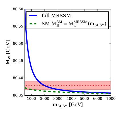
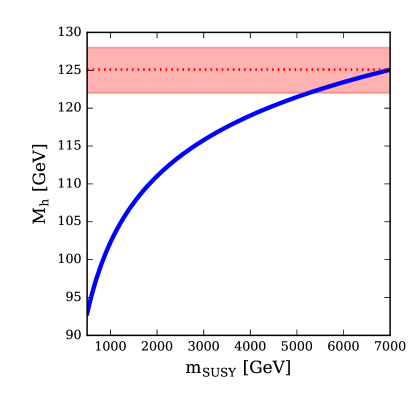
Figure 1: Comparison of the $M_{W}$ ($M_{h}$) prediction as blue full line on the left (right) depending on a common SUSY mass scale $m_{\text{SUSY}}$ (definition given in the text). The green dashed line on the left shows the prediction of the SM calculation for $M_{W}$ if $M_{h}^{\text{SM}}=M_{h}^{\text{MRSSM}}(m_{\text{SUSY}})$ is used. The red dotted line and the shaded area show on the left the experimental central value for $\MW$ and its 1 $\sigma$ uncertainty band according to eq. (3), while on the right the experimental value for the mass of the detected Higgs boson is supplemented by a band of $\pm 3\leavevmode\nobreak\ \text{GeV}$ indicating a rough estimate of theoretical uncertainties from unknown higher-order corrections. All dimensionless superpotential parameters are chosen as for BMP1 of ref. PD2 .

We investigate the decoupling behaviour for $M_{W}$ by defining a general SUSY mass scale $m_{\text{SUSY}}$ as follows for the soft breaking parameters of eqs. (8) and (9) as well as the $\mu_{d}$ and $\mu_{u}$ parameter of the superpotential:

$$m^{2}_{R_{u}}=m^{2}_{R_{d}}=m_{S}^{2}=m_{T}^{2}=m_{O}^{2}=2\frac{B_{\mu}}{\sin 2\beta} =m_{\text{SUSY}}^{2}\;,$$

$$m^{2}_{\tilde{q},L}=m^{2}_{\tilde{l},L}=m^{2}_{\tilde{e},R}=m^{2}_{\tilde{u},R}=m^{2}_{\tilde{d},R} =m_{\text{SUSY}}^{2}\cdot\mathbf{1}\;,$$

$$M^{D}_{B}=M^{D}_{W}=M^{D}_{O}=\mu_{d}=\mu_{u} =\frac{m_{\text{SUSY}}}{2}\;.$$ (47)

The superpotential parameters are fixed to the value of the benchmark point BMP1 given in ref. PD2 ; Diss , the dimensionless couplings are set as $\Lambda_{d}=-1$, $\Lambda_{u}=-1.03$, $\lambda_{d}=1.0$ and $\lambda_{u}=-0.8$. The ratio of the doublet vevs has been set to $\tan\beta=3$.

In figure 1 we show the dependence of $M_{W}$ and $M_{h}$ on the common SUSY mass scale $m_{\text{SUSY}}$ defined above. The mass splitting between fermionic and bosonic mass parameters is required to achieve a prediction for the SM-like Higgs boson mass $M_{h}$ close to the experimental value measured at the LHC. The MRSSM prediction for $M_{h}$ is shown on the right-hand side of fig. 1. The prediction for $\MW$ in the MRSSM is compared in the left plot with the SM prediction for $\MW$ where the mass of the Higgs boson in the SM is identified with the corresponding MRSSM prediction for the mass of the SM-like Higgs boson, $M_{h}^{\text{SM}}=M_{h}^{\text{MRSSM}}(m_{\text{SUSY}})$. It can be seen that with a rising SUSY mass scale the SUSY contributions decouple, and the prediction for $M_{W}$ approaches the SM limit for large SUSY masses. On the other hand, for small values of $m_{\text{SUSY}}$ the prediction for $\MW$ shows a steep rise while the prediction for $M_{h}$ is significantly lowered. As one can infer from a comparison of the two curves in the left plot, the effect of shifting the value of the Higgs-boson mass in the SM-type contributions accounts only for a a small fraction of the increase in $\MW$ for small $m_{\text{SUSY}}$, while the bulk of the effect is caused by generic MRSSM contributions.

The comparison of the behaviour of the prediction for $\MW$ in figure 1 with the case of the MSSM and the NMSSM (see e.g. refs. Heinemeyer:2006px ; Stal:2015zca ) shows that in the MRSSM the decoupling to the SM result occurs at higher values of the SUSY mass scale, while the increase of $\MW$ for a decreasing SUSY scale is more pronounced than in the MSSM and the NMSSM. The difference between the MRSSM prediction and the SM prediction with $M_{h}^{\text{SM}}=M_{h}^{\text{MRSSM}}(m_{\text{SUSY}})$ still amounts to about 10 MeV for $m_{\text{SUSY}}$ values of about 3 TeV in figure 1, and the difference reduces to values below 1 MeV only for $m_{\text{SUSY}}\;\raisebox{-3.00003pt}{$\stackrel{{\scriptstyle\displaystyle>}}{{\sim}}$}\;5\leavevmode\nobreak\ \text{TeV}$. The different behaviour in the MRSSM as compared to the MSSM and the NMSSM Heinemeyer:2006px ; Stal:2015zca is in particular related to the enlarged matter content in the MRSSM, where the additional degrees of freedom arise from the adjoint and the R-Higgs superfields, and to the fact that the $\Lambda/\lambda$ superpotential parameters contribute to $M_{W}$ in a similar way as the top Yukawa coupling. In the considered scenario the $\Lambda_{u/d}$ couplings are of order one and have a large effect on the prediction. For low SUSY masses the triplet vev has a relevant influence on $M_{W}$ already at tree-level. The impact of the triplet vev becomes negligible for larger SUSY mass scales as $v_{T}$ goes to zero, see the discussion in section 3.1.2.

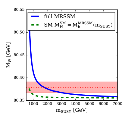
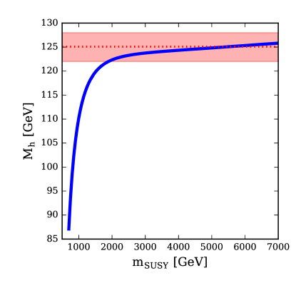
Figure 2: As figure 1 but with $\mu_{d}=\mu_{u}$ fixed to $400$ GeV.

In the simplified scenario with a common mass scale $m_{\text{SUSY}}$ of figure 1 one can see that the range of $m_{\text{SUSY}}$ values yielding a prediction for $\MW$ within the $1\sigma$ band of the experimental central value does not coincide with the parameter region where the mass of the SM-like Higgs boson is close to 125 GeV. The prediction for $M_{h}$ in the MRSSM has a significant dependence on the parameters $\mu_{d}$ and $\mu_{u}$. This can be seen in figure 2 where the same parameters as in figure 1 are used except that $\mu_{d}$ and $\mu_{u}$ are not scaled with $m_{\text{SUSY}}/2$ as in eq. (47) but kept fixed at $\mu_{d}=\mu_{u}=400$ GeV. For fixed values of $\mu_{d}$ and $\mu_{u}$ the MRSSM prediction for $\MW$ still approaches the SM prediction for large values of $m_{\text{SUSY}}$, but the numerical difference between the two predictions remains sizeable up to even higher values of $m_{\text{SUSY}}$ than in figure 1. On the other hand, the fixed value of $\mu_{d}=\mu_{u}=400$ GeV brings the regions of $m_{\text{SUSY}}$ that are preferred by the $\MW$ and $M_{h}$ predictions into better agreement with each other.

5.2 Impact of different MRSSM contributions

In the following we investigate how the different contributions in the MRSSM affect $M_{W}$ separately. First we describe the influence of the triplet vev on the prediction for $M_{W}$. Then we describe how the different MRSSM sectors contribute to $M_{W}$ individually. Especially the extended Higgs and neutralino sectors are relevant in this context as they differ in the MRSSM from the MSSM and NMSSM and contain the effects from the $\Lambda/\lambda$ couplings. Several of the figures shown in the following sections contain plots of both $M_{W}$ and $M_{h}$ as function of the parameters of interest. This is of interest as the Higgs boson mass in the MRSSM is very sensitive to those parameters, and as shown in figure 1 the variation of $M_{h}$ has an impact on $M_{W}$ via the SM-type contributions. In order to disentangle this contribution from the genuine MRSSM effects it is convenient to also show the dependence of $M_{h}$ on the relevant parameters.

The fixed parameters are set either as before, when $m_{\text{SUSY}}$ is varied, or we use updated values for BMP1 of ref. PD2 giving rise to a better agreement with the latest experimental value for $M_{W}$ given in (3). The latter parameters are

$$\tan\beta =3,\;\Lambda_{d}=-1.2,\;\Lambda_{u}=-1.1,\;\lambda_{d}=1.0,\;\lambda_{u}=-0.8,$$

$$\mu_{u} =\mu_{d}=500\text{ GeV},\;M_{B}^{D}=550\text{ GeV},\;M_{W}^{D}=600\text{ GeV},\;m_{R_{d}}=m_{R_{u}}=m_{S}=2\text{ TeV},$$

$$M_{O}^{D} =1.5\text{ TeV},\;m_{\tilde{l},L}=m_{\tilde{e},R}=1\text{ TeV},m_{O}=m_{\tilde{q},L;3}=m_{\tilde{u},R;3}=m^{2}_{\tilde{d},R;3}=1.5\text{ TeV},\;$$

$$B_{\mu} =(500\text{ GeV})^{2},\;m_{T}=3\text{ TeV},\;m_{\tilde{q},L;1,2}=m_{\tilde{u},R;1,2}=m_{\tilde{d},R;1,2}=2.5\text{ TeV}\;.$$ (48)

5.2.1 Influence of the triplet vev

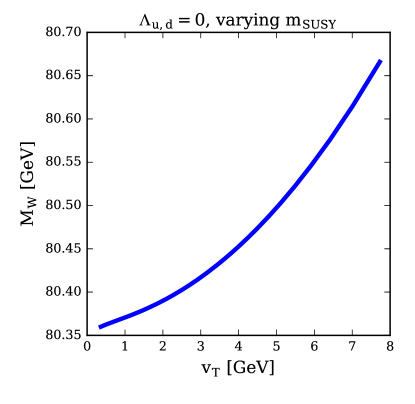
Figure 3: Dependence of $M_{W}$ on $v_{T}$ obtained from varying the common SUSY mass scale as in figure 1.

As the triplet vev affects the W boson mass already at the tree level by breaking custodial symmetry, even a small value (compared to $M_{W}$) affects the prediction at the same order as the size of the experimental uncertainty.

In figure 3 we show the interplay of $v_{T}$ and $M_{W}$ when the SUSY mass scale $m_{\text{SUSY}}$ is varied as in figure 1 and all $\lambda_{d,u}/\Lambda_{d,u}$ are set equal to zero. One can see that in this case the $v_{T}$ tree level contribution is numerically large for $v_{T}\;\raisebox{-3.00003pt}{$\stackrel{{\scriptstyle\displaystyle>}}{{\sim}}$}\;1$ GeV. The potentially large impact of $v_{T}$ can be clearly seen by the quadratic dependency exhibited in the figure which is in accordance with eq. (14). For $|v_{T}|\;\raisebox{-3.00003pt}{$\stackrel{{\scriptstyle\displaystyle>}}{{\sim}}$}\;3$ GeV the prediction for $M_{W}$ grows above the experimentally allowed region. Therefore, for phenomenological reasons the parameter region with $|v_{T}|\;\raisebox{-3.00003pt}{$\stackrel{{\scriptstyle\displaystyle<}}{{\sim}}$}\;3$ GeV is preferred. For $|v_{T}|\approx 3$ GeV, using the parameters of eq. (48) and adjusting $m_{T}$ accordingly, the associated one-loop contribution (which is proportional to $v_{T}^{2}$) to $\Delta\tilde{r}$ from eq. (27) is of similar size as the SM three- and four-loop contributions leading to a shift of $\delta M_{W}^{(v_{T}),\text{Loop}}\approx 1\text{ MeV}$. It should be noted that the higher-order contributions also significantly depend on the SUSY mass spectrum.

For our numerical analysis in the following we choose the parameters of eq. (48) as basis. This yields

$$v_{T}^{\overline{\text{DR}}}(Q=m_{\text{SUSY}})=-0.38\leavevmode\nobreak\ \text{GeV}$$ (49)

as an input for our $M_{W}$ calculation. This setting leads to a a tree-level (one-loop) shift of $\delta M_{W}^{(v_{T})}=0.28$ MeV ($\delta M_{W}^{(v_{T})}=-0.17$ MeV), respectively, where again it should be noted that the higher-order contributions are significantly affected by the parameters of the SUSY mass spectrum.

5.2.2 Influence of the $\Lambda$ couplings

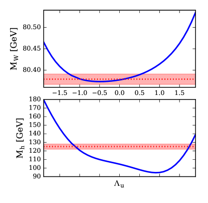
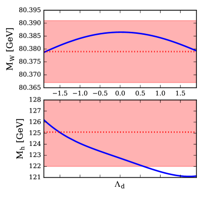
Figure 4: Dependence of $M_{W}$ and $M_{h}$ on $\Lambda_{d}$ and $\Lambda_{u}$. The value for $v_{T}$ is fixed according to eq. (49), and the other model parameters are chosen as in eq. (48). The red bands mark the experimental (theoretical) uncertainty region for $M_{W}$ ($M_{h}^{\text{SM-like}}$) as in figure 1.

The dependence of $M_{W}$ on the superpotential parameters $\Lambda_{d}$ and $\Lambda_{u}$ is shown in figure 4. The effects are stronger for $\Lambda_{u}$ than for $\Lambda_{d}$ because of $\tan\beta>1$. In the extreme case of $\Lambda_{u}=2$ a shift of more than $\delta M_{W}^{(\Lambda_{u})}=130$ MeV is possible compared to the minimal value at $\Lambda_{u}=-0.5$. In the phenomenologically interesting region where the MRSSM Higgs boson mass prediction is around the experimental observation of about $125$ GeV with $\Lambda_{u}=-1.1$ the shift in $M_{W}$ compared to $\Lambda_{u}=0$ is $\delta M_{W}^{(\Lambda_{u})}\approx 10$ MeV. The actual effect from the $\Lambda_{u}$ variation on $M_{W}$ for large $|\Lambda_{u}|$ is even stronger than the variation displayed in figure 4 since large $|\Lambda_{u}|$ also drives the SM Higgs mass prediction to values far above the experimental observation, as shown in the lower left plot of figure 4, which gives rise to a downward shift from the SM-type part of the contributions to $M_{W}$. As shown on the right-hand side of figure 4, an enhancement of the magnitude of $\Lambda_{d}$ from zero to unity leads to a reduction of $\delta M_{W}^{(\Lambda_{d})}=-5$ MeV, while the prediction for $M_{h}$ is lowered by about 1 GeV.

The behaviour of $M_{W}$ with regard to the two parameters $\Lambda_{d}$ and $\Lambda_{u}$ can be understood from their influence on the electroweak precision parameters $S$, $T$ and $U$ which contribute to $M_{W}$. For this, we follow the lines of refs. PD1 ; Diss . There, several limits of the contributions to $S$, $T$ and $U$ were studied analytically. The $T$ parameter has been identified as the one with the biggest impact on $M_{W}$, where the contributions from the neutralino and chargino sector dominate. Up to a prefactor the definition of the $T$ parameter corresponds to the one of $\Delta\rho$. In general, the $\Delta\rho$ parameter depends on the fourth power of $\Lambda$ leading to significant effects for magnitudes close to or above unity, as it is visible in figure 4.

It is of interest to understand the interplay of $\Lambda_{d}$ and $\Lambda_{u}$ concerning the $M_{W}$ prediction. In the previous works of refs. PD1 ; Diss , all analytical expressions in the study of several model limits have been derived setting $v_{d}=0$, turning off all $\Lambda_{d}$ contributions. As we want to investigate these contributions we discuss a different model limit in the following. We take the gaugeless limit ($g_{1}=g_{2}=0$) and set $\mu_{d}=\mu_{u}=M^{D}_{W}$ and $\lambda_{u}=\lambda_{d}=0$. Then, we find contributions from the electroweakino sector to the $\Delta\rho$ parameter as

$$\Delta\rho_{0}^{\Lambda}=\frac{\alpha}{16\pi M_{W}^{2}\tilde{s}_{W}^{2}}\frac{13\left(\Lambda_{u}^{2}v_{u}^{2}-\Lambda_{d}^{2}v_{d}^{2}\right)^{2}}{96(M_{W}^{D})^{2}}.$$ (50)

The relative sign between the two couplings and the fact that $\tan\beta>1$ for the scenario considered is the reason why an increase of $\Lambda_{d}^{2}$ actually decreases the prediction for $M_{W}$ when $\Lambda_{d}$ and $\Lambda_{u}$ are of similar magnitude. The $\Lambda_{u}$ contribution dominates for most of the parameter space, and the $\Lambda_{d}^{2}$ term leads to a reduction of the contribution in this case. The situation is reversed for $\tan\beta<1$.

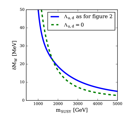
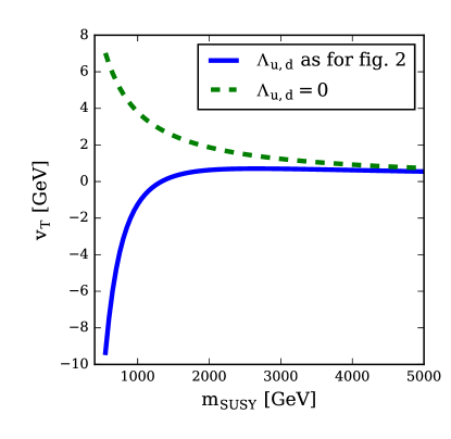
Figure 5: The plot on the left depicts the shift in the prediction of $M_{W}$ with respect to the SM prediction according to eq. (51). On the right the corresponding value of $v_{T}$ is plotted. Two different scenarios are considered where the parameters $\Lambda_{d,u}$ are fixed to either the values $\Lambda_{d}=-1$, $\Lambda_{u}=-1.03$ or to zero, while $\mu_{d}=\mu_{u}=500$ GeV, and the values of all other mass parameters are given in eq. (47).

In figure 5 we show on the left the quantity

$$\delta M_{W}=M_{W}^{\text{MRSSM}}-M^{W}_{\text{SM}}(M_{H}^{\text{SM}}=M_{h}^{\text{MRSSM}}(m_{\text{SUSY}}))\,,$$ (51)

where as above $M_{h}^{\text{MRSSM}}$ is the SM-like Higgs boson mass of the MRSSM. On the right the prediction for $v_{T}$ is depicted. We compare the scenario studied above where the magnitudes of $\Lambda_{d,u}$ are of order unity with a scenario where $\Lambda_{d}$ and $\Lambda_{u}$ are both fixed to zero. Note that it is necessary to fix the values of $\mu_{d}$ and $\mu_{u}$ to the ones of the benchmark point of eq. (48), while all other dimensionful SUSY parameter are scaled with $m_{\text{SUSY}}$ as specified in eq. (47). The parameters $\lambda_{d}$ and $\lambda_{u}$ are also set as in eq. (48). This setting limits the size of $v_{T}$ for $m_{\text{SUSY}}$ below 1 TeV. In both scenarios the difference in the prediction for $M_{W}$ between the MRSSM and the SM decreases from more than $50$ MeV at $m_{\text{SUSY}}\approx 1$ TeV to below 5 MeV for $m_{\text{SUSY}}$ values in the multi-TeV range. Both lines show a very similar shape while the main contributions to $\delta M_{W}$ are different in the two scenarios.

In the scenario with $\Lambda_{d,u}$ of about $-1$ the magnitude of the triplet vev drops to below 1 GeV for $m_{\text{SUSY}}>1$ TeV as there is a partial cancellation in the numerator of eq. (41) between the terms of $\Lambda_{u/d}\mu_{u/d}$ and $g_{2}M_{W}^{D}$, which are of similar magnitude. Therefore, $v_{T}$ drops below 1 GeV already for relatively low $m_{\text{SUSY}}$. It goes to zero for larger $m_{\text{SUSY}}$ but with a smaller rate as the cancellation in the numerator of eq. (41) is not perfect. As $v_{T}$ is small above $m_{\text{SUSY}}=1$ TeV, its tree-level contribution does not substantially impact the prediction for $M_{W}$ in this parameter region. Then, loop corrections from $\Lambda_{d,u}$ like eq. (50) are the most relevant ones.

In the scenario where $\Lambda_{d,u}$ are fixed to zero their loop contributions vanish. On the other hand, there is no significant cancellation in the numerator of eq. (41) for $\tan\beta\gg 1$. Then, $v_{T}$ drops below 1 GeV only above $m_{\text{SUSY}}=3.5$ TeV, and its tree-level contribution to $M_{W}$ is relevant for a larger mass range.

5.2.3 Higgs sector contributions

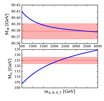
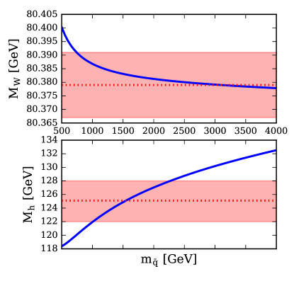
Figure 6: Dependence of $M_{W}$ and $M_{h}$ on a common Higgs sector mass (left) and a common squark mass (right). The other parameters are chosen as in figure 4.

In the following, we investigate the influence of the extended Higgs sector of the MRSSM on the W boson mass. The contributions from the Higgs sector include the ones from the two MSSM-like Higgs doublets, the singlet and triplet states, which all mix with each other, as well as the two R-Higgs doublets. We vary all the relevant soft breaking masses $m_{S}^{2}$, $m_{T}^{2}$, $m_{R_{u/d}}^{2}$ as well as the MSSM-like CP-odd Higgs mass parameter $m_{A}^{2}=2B_{\mu}/\sin 2\beta$ simultaneously to show the dependence of the W boson mass on them. On the left side of figure 6 the dependences of $M_{W}$ and $M_{h}$ on these parameters are shown. As a comparison we show the dependence on the squark masses on the right, here all the soft-breaking squark mass parameters are varied simultaneously.

Altogether, varying the common Higgs sector mass from 500 GeV to 4 TeV leads to an increase of the Higgs boson mass by almost 30 GeV and a simultaneous decrease of $M_{W}$ by about 30 MeV. The variation of the common squark mass from 500 GeV to 4 TeV on the other hand increases the Higgs boson mass by about 14 GeV while $M_{W}$ drops by about 20 MeV. For both plots decoupling-like behaviour of the relevant SUSY contributions to $\MW$ can be seen which is similar to the one in figure 1. The residual slope for high SUSY masses originates purely from the Higgs mass dependence of the SM-like contributions to $\Delta\tilde{r}$.

It has been noted before PD1 that ${\cal O}(1)$ $\lambda/\Lambda$ parameters have effects comparable to the ones of the top Yukawa coupling as both, the Yukawa and $\lambda/\Lambda$ couplings, originate from similar terms of the superpotential. The squark contributions to $M_{W}$ stem mainly from top-Yukawa effects with a suppression factor originating from the squark masses. The Higgs sector effects on the other hand are driven by the $\lambda/\Lambda$ parameters being of order one and are suppressed by the soft-breaking Higgs mass terms. Therefore, the similar behaviour arising from both sectors for $M_{W}$ and $M_{h}$ as shown in figure 6 is expected. The effect of the Higgs sector is quantitatively larger when varying the involved common mass parameters in a similar range as more degrees of freedom contribute in the Higgs sector even taking into account the colour factor for the squark contributions. A rising $m_{T}$ leads to a suppression of the triplet vev and its contribution to $M_{W}$ via the tadpole relation (41).

5.2.4 Neutralino contributions

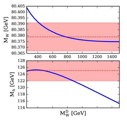
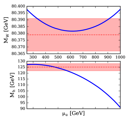
Figure 7: Dependence of $M_{W}$ and $M_{h}$ on $M^{D}_{W}$ (left) and $\mu_{u}$ (right). The other parameters are chosen as in figure 4.

Contributions of charginos and neutralinos to $M_{W}$ are very relevant in the MRSSM as the $\Lambda$ superpotential parameters affect their mixing and lead to novel contributions. Additionally, the dimensionful parameters influence these corrections directly and indirectly, which is discussed in the following.

Figure 7 (left) shows that the effect of the mass parameter $M^{D}_{W}$ is similar to the ones of the scalar soft breaking masses discussed before, i.e. the predicted value for $M_{W}$ decreases for rising $M^{D}_{W}$. As already noted in the discussion of figure 1 and figure 2, the parameter $\mu_{u}$ has a large impact on the prediction for $M_{h}$ in the MRSSM. In the plots on the right-hand side of figure 7 the variation of $\mu_{u}$ is only shown in the range of $250$ to $1000$ GeV as for higher values of $\mu_{u}$ the tree-level Higgs boson mass becomes tachyonic. This is caused by the effect of $\mu_{u}$ on the singlet–doublet mixing of the scalar Higgs boson mass matrix in the form $\mathcal{M}_{13}^{\text{CP-even}}=-v_{u}(\sqrt{2}\lambda_{u}\mu_{u}^{\text{eff,}-}+g_{1}M^{D}_{B})$. Because the SM-like Higgs boson is the lightest electroweak scalar in the considered scenario, the enhanced mixing leads to a strong reduction of the Higgs boson mass and the appearance of a tachyonic state for large $\mu_{u}$. The Higgs boson mass also decreases with rising $M^{D}_{W}$ as the loop contributions to $M_{h}$ depend on $\log(m_{T}/M^{D}_{W})$. As the Dirac mass is smaller than the scalar mass in the considered range the Higgs boson mass decreases with increasing $M^{D}_{W}$.

Varying $M^{D}_{W}$ and $\mu_{u}$ in the mass range from 250 to 600 GeV yields a downward shift in the $M_{W}$ prediction of $\delta M_{W}^{(M^{D}_{W})}=21$ MeV for $M^{D}_{W}$ and $\delta M_{W}^{(\mu_{u})}=16$ MeV for $\mu_{u}$. The downward shifts are mainly driven by contributions from $\Delta\rho_{0}^{\Lambda}$, see eq. (50). For the mass range above about $600$ GeV the prediction for the mass of the SM-like Higgs boson decreases for both parameters, as described above. In this parameter region the decrease in the Higgs boson mass leads to additional contributions shifting $\MW$ upwards. Those contributions from the SM-like Higgs boson partially cancel the SUSY corrections, with a net effect in the $M_{W}$ prediction of a less steep decrease with rising $M^{D}_{W}$ and of an increase with rising $\mu_{u}$.

5.3 Scan over MRSSM parameters

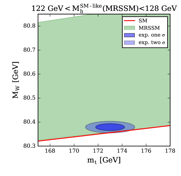
Figure 8: Prediction for the W boson mass in the MRSSM and the SM versus the input value of the top quark pole mass in comparison with the experimental results for $\MW$, see eq. (3), and $m_{t}$, see eq. (5). The green band of MRSSM predictions arises from the scan over MRSSM parameters specified in eq. (52), where the condition $122\leavevmode\nobreak\ \text{GeV}<M_{h}<128\leavevmode\nobreak\ \text{GeV}$ has been applied for the prediction of the SM-like Higgs boson mass. The narrow red band, which is shown on top of the green band, indicates the SM prediction where the experimental measurement is used as input for the Higgs boson mass. For the experimental measurements of $\MW$ and $m_{t}$ the two-dimensional regions allowed at the 1 $\sigma$ and the 2 $\sigma$ level are indicated.

In figure 8 we show the predictions for $\MW$ in the MRSSM resulting from a scan over MRSSM parameters as a green band in relation to the input value for the top quark pole mass. We have arrived at this band by scanning over several parameter combinations,

$$-1.5 <-\lambda_{d}=\Lambda_{d}=\lambda_{u}=\Lambda_{u}<1.5\;,$$

$$250\text{ GeV} <\mu_{d}=\mu_{u}=M^{D}_{B}=M^{D}_{W}<3000\text{ GeV}\;,$$

$$250\text{ GeV} <m_{S}=m_{T}=m_{R_{d}}=m_{R_{u}}=m_{A}<3000\text{ GeV}\;,$$

$$250\text{ GeV} <m_{\tilde{q},L}=m_{\tilde{l},L}=m_{\tilde{d},R}=m_{\tilde{u},R}=m_{\tilde{e},R}<3000\text{ GeV}\;,$$ (52)

where the prediction for the mass of the SM-like Higgs boson has been required to agree with the measured value within the theoretical uncertainties. As condition for $M_{h}$ the mass range $122\leavevmode\nobreak\ \text{GeV}<M_{h}<128\leavevmode\nobreak\ \text{GeV}$ has been adopted. The SM prediction where the measured Higgs boson mass within the experimental uncertainties has been used as input is shown in red. The blue ellipses mark the measurements of the top quark and the W boson mass including their two-dimensional 1 $\sigma$ and 2 $\sigma$ experimental uncertainty regions. It should be noted that the systematic uncertainty in relating the measured value of the top quark mass to the top quark pole mass (see the discussion above) is not accounted for in figure 8. A proper inclusion of this uncertainty would widen the displayed ellipses along the $m_{t}$ axis.

The comparison of the MRSSM and SM predictions for $\MW$ with the experimental results for $\MW$ and $m_{t}$ in figure 8 shows on the one hand that MRSSM parameter regions giving rise to a large upward shift in $\MW$ as compared to the SM case are disfavoured by the measured value of $\MW$, in accordance with the results of figures 1–7. On the other hand, figure 8 indicates a slight preference for a non-zero SUSY contribution to $\MW$, see also the discussion for the MSSM and the NMSSM in refs. Heinemeyer:2006px ; Heinemeyer:2013dia . The band of the SM prediction barely intersects with the 2 $\sigma$ ellipse of the experimental results in figure 8, and a non-zero SUSY contribution giving rise to a moderate upward shift in $\MW$ is required in order to reach compatibility with the experimental result at the 1 $\sigma$ level.

5.4 Comparison to other calculation methods

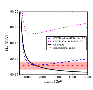
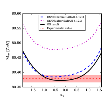
Figure 9: Comparison of the $M_{W}$ prediction as a function of $m_{\text{SUSY}}$ (left) and $\Lambda_{u}$ (right) calculated in this work using the on-shell scheme (black line) with the result from SARAH/SPheno using the original contributions (blue dashed line) and using corrected contributions (purple dash-dotted line). As in the figures above, the red dotted line and the shaded area show the experimental central value for $\MW$ and its 1 $\sigma$ uncertainty band according to eq. (3). All other model parameters are chosen as for BMP1 of ref. PD2 . For details see the discussion in the text.

After the discussion of the various features of our numerical results, we now turn to a comparison of our results with predictions for $\MW$ in the MRSSM that have been obtained with other approaches. As discussed above, the calculation of $M_{W}$ in refs. PD1 ; PD2 ; PD3 was done using the implemented mixed OS/$\overline{\text{DR}}$ calculation of SARAH/SPheno. In ref. Athron:2017fvs and the update of the program FlexibleSUSY, it was recently shown that SM higher-order contributions implemented in SARAH/SPheno were not correct with regard to the usage of the OS and $\overline{\text{DR}}$ top quark mass in the two-loop SM contribution. Correcting the implementation leads to a shift of $M_{W}$ of 50–100 MeV compared to the result of the original calculation for example given in refs. PD1 ; PD2 ; PD3 for the MRSSM. This is not only true for the MRSSM but also for all other versions of SARAH/SPheno and also concerns the original SPheno code. In the following we show how the on-shell calculation presented here compares to the previous and corrected mixed OS/$\overline{\text{DR}}$ scheme predictions obtained with SARAH/SPheno.

In figure 9 we show the predictions for $M_{W}$ arising from the different calculations as function of the common SUSY mass scale as defined in section 5.1 (left) and of the superpotential parameter $\Lambda_{u}$ of the MRSSM (right). The on-shell result obtained in this work is given as solid black line, the previous OS/$\overline{\text{DR}}$ result as dashed blue line and the corrected OS/$\overline{\text{DR}}$ result as dash-dotted purple line. The experimental result for $\MW$ is shown as red dotted line with a shaded region for the experimental 1 $\sigma$ uncertainty.

It can be seen in the left plot of figure 9 that only the on-shell result presented in this work shows a proper decoupling behaviour where for large $m_{\text{SUSY}}$ the MRSSM prediction approaches the SM prediction in which the Higgs boson mass of the SM is identified with the mass of the SM-like Higgs boson of the MRSSM, see also figure 1. Both the previous and corrected mixed OS/$\overline{\text{DR}}$ scheme predictions obtained with SARAH/SPheno show a slope for large $m_{\text{SUSY}}$ such that the deviation between the MRSSM prediction and the SM prediction grows for increasing $m_{\text{SUSY}}$. The correction of the contributions for the OS/$\overline{\text{DR}}$ calculation yields a large upward shift of about 100 MeV in $\MW$ that is roughly constant for the displayed range of $m_{\text{SUSY}}$. As a consequence, the prediction for $\MW$ arising from the calculation in the mixed OS/$\overline{\text{DR}}$ scheme including the correction shows a large deviation from the measured value of $\MW$ for all values of $m_{\text{SUSY}}$. The same feature also holds for the plot as function of $\Lambda_{u}$ shown on the right-hand side of figure 9. Also in this case the correction that was implemented in the calculation based on the mixed OS/$\overline{\text{DR}}$ scheme yields a roughly constant upward shift in $\MW$ that brings the MRSSM prediction far away from the experimental result for $\MW$. Both the previous and corrected SARAH/SPheno predictions agree with the corresponding results from FlexibleSUSY generator shown on the right of Fig. 10 in ref. Athron:2017fvs . Thus, the large deviation observed in the results for the MSSM and the MRSSM based on the mixed OS/$\overline{\text{DR}}$ scheme appears to be a general feature of this scheme.

In view of these findings the relatively good agreement between our on-shell result and the previous mixed OS/$\overline{\text{DR}}$ scheme prediction obtained with SARAH/SPheno before the correction (dashed blue line) for $m_{\text{SUSY}}$ below $2$ TeV (left plot) and for the whole $\Lambda_{u}$ range (right plot) appears to be a numerical accident. This accidental agreement implies that the parameter regions that were identified in refs. PD1 ; PD2 ; PD3 for predicting $M_{W}$ values that are compatible with the experimental result are roughly in agreement with the ones obtained from our new on-shell prediction within the estimated uncertainties. We have verified this accidental feature for the benchmark points of the MRSSM proposed in refs. PD1 ; PD2 ; PD3 . Further investigations to clarify the observed features of the mixed OS/$\overline{\text{DR}}$ scheme prediction, which has been first proposed for the MSSM in ref. BPMZ and most generally been implemented in the tools SARAH/SPheno and FlexibleSUSY, would clearly be desirable.

6 Conclusions

We have presented the currently most accurate prediction for the mass of the W boson in the MRSSM. The result is based on the on-shell scheme, using the muon decay constant, the fine-structure constant and the Z boson pole mass as precisely measured experimental inputs. The appearance of a triplet scalar vacuum expectation value $v_{T}$ at lowest order in the electroweak symmetry breaking condition for the W boson mass but not in the corresponding relation for the mass of the Z boson leads to custodial symmetry breaking effects in the prediction for $M_{W}$ already at tree-level, while the other BSM parameters of the MRSSM enter via higher-order corrections. As described in detail, the prediction for the W boson mass needs to properly take into account the relation between the weak mixing angle and the gauge boson masses that is modified in the MRSSM in comparison to the SM and extensions of it involving only Higgs doublets and singlets.

Our prediction for the W boson mass is based on the full one-loop contributions in the MRSSM that we have supplemented by all available SM-type corrections of higher order. The implementation is based on a SPheno-4.0.3 mass spectrum generator that has been obtained by SARAH-4.12 for the MRSSM. The calculation of $M_{W}$ in the on-shell scheme has been carried out making use of the available analytical one-loop expressions that have been consistently combined with the high-order corrections of SM-type. For the latter a fit formula has been implemented, which accounts for the full electroweak two-loop corrections of SM-type involving numerical integrations of two-loop integrals with non-vanishing external momenta, as well as analytical results for leading QCD, electroweak and mixed corrections up to the four-loop level. For the renormalisation of the triplet scalar vacuum expectation value $v_{T}$ entering the prediction for $\MW$ at lowest order a $\overline{\text{DR}}$-type prescription has been chosen, where the numerical value is determined via a two-step procedure ensuring numerical stability.

We have investigated the numerical result for the W boson mass in view of the characteristics of the parameter space of the MRSSM. We have verified in this context that in the decoupling limit where the SUSY particles are heavy the SM prediction is recovered, i.e. in this limit the MRSSM result approaches the SM prediction in which the Higgs boson mass of the SM is identified with the mass of the SM-like Higgs boson of the MRSSM. The upward shift in $\MW$ for a small SUSY mass scale tends to be more pronounced in the MRSSM than it is the case in the MSSM and the NMSSM, while the decoupling to the SM result occurs at higher values of the SUSY mass scale than in those models.

The most relevant SUSY parameters of the MRSSM influencing the prediction for $M_{W}$ are the triplet vacuum expectation value and the $\Lambda$ superpotential couplings. The triplet vacuum expectation value is related to all other model parameters through its contribution to the electroweak symmetry breaking conditions and gives rise to a lowest-order shift in the $\rho$ parameter. Since the $\Lambda$ parameters are trilinear couplings of the superpotential, they enter in a similar way as the Yukawa couplings, see also the discussion in ref. PD1 . We have identified leading contributions to the prediction for $\MW$ that enter with the fourth power of $\Lambda_{u}$ and $\Lambda_{d}$. Additionally, the $\Lambda$ couplings have an important impact via the contributions of the neutralino and chargino sector to $M_{W}$. The contributions to $M_{W}$ of the extended Higgs sector of the MRSSM with a common Higgs sector mass show a qualitatively similar behaviour as the ones of the squark sector with a common squark mass. Confronting the results of a parameter scan in the MRSSM as well as the SM prediction for $\MW$ as a function of $m_{t}$ with the experimental results for the W boson mass and the top quark mass, we have demonstrated a slight preference for a non-zero SUSY contribution to $\MW$. While this preference is similar to the results that were found in the MSSM and the NMSSM, it should be noted that there is no direct limit from the MRSSM to the MSSM. This is caused in particular by the fact that the $\Lambda$ couplings are a specific feature of the MRSSM and by the pure Dirac nature of gauginos and Higgsinos in the MRSSM. While certain contributions are similar in the two models, in particular the MSSM-like contributions from stops and sbottoms which are driven by the top Yukawa coupling, the absence of trilinear A-terms in the MRSSM also gives rise to differences in the squark sector.

We have compared our results for $\MW$ to the ones that were obtained in the MRSSM from the mixed OS/$\overline{\text{DR}}$ implementation of SARAH/SPheno before PD1 ; PD2 ; PD3 and after the correction that was pointed out in ref. Athron:2017fvs was carried out. While as described above our result shows a proper decoupling behaviour where for large values of a common SUSY mass scale in the MRSSM the SM prediction is recovered, this is not the case for either of the previous results. Those predictions show a deviation from the SM result that actually grows with increasing $m_{\text{SUSY}}$. While the result of the mixed OS/$\overline{\text{DR}}$ implementation of SARAH/SPheno before the correction was applied agrees relatively well with our result in some parts of the parameter space, a feature that is apparently caused by a numerical coincidence, the mixed OS/$\overline{\text{DR}}$ implementation of SARAH/SPheno including the correction shows a large upward shift in $\MW$ of about 100 MeV compared to the previous result that gives rise to a large deviation from the measured value of $\MW$. Because of the described accidental numerical agreement our analysis roughly confirms the preferred MRSSM parameter regions that were identified from the investigation of the $M_{W}$ prediction in refs. PD1 ; PD2 . As we have demonstrated, the large deviations of the result of the mixed OS/$\overline{\text{DR}}$ implementation of SARAH/SPheno including the correction both with respect to our result and with respect to the experimental value of $\MW$ should motivate further work in this direction.

References

- (1) ATLAS Collaboration collaboration, G. Aad et al., Observation of a new particle in the search for the Standard Model Higgs boson with the ATLAS detector at the LHC, Phys.Lett. B716 (2012) 1–29, [1207.7214].
- (2) CMS collaboration, S. Chatrchyan et al., Observation of a new boson at a mass of 125 GeV with the CMS experiment at the LHC, Phys.Lett. B716 (2012) 30–61, [1207.7235].
- (3) ATLAS, CMS collaboration, G. Aad et al., Combined Measurement of the Higgs Boson Mass in Collisions at and 8 TeV with the ATLAS and CMS Experiments, 1503.07589.
- (4) G. D. Kribs and A. Martin, Supersoft Supersymmetry is Super-Safe, Phys. Rev. D85 (2012) 115014, [1203.4821].
- (5) G. D. Kribs, E. Poppitz and N. Weiner, Flavor in supersymmetry with an extended R-symmetry, Phys.Rev. D78 (2008) 055010, [0712.2039].
- (6) P. Dießner, J. Kalinowski, W. Kotlarski and D. Stöckinger, Higgs boson mass and electroweak observables in the MRSSM, JHEP 12 (2014) 124, [1410.4791].
- (7) P. Diessner, J. Kalinowski, W. Kotlarski and D. Stöckinger, Two-loop correction to the Higgs boson mass in the MRSSM, Adv. High Energy Phys. 2015 (2015) 760729, [1504.05386].
- (8) P. Diessner, J. Kalinowski, W. Kotlarski and D. Stöckinger, Exploring the Higgs sector of the MRSSM with a light scalar, JHEP 03 (2016) 007, [1511.09334].
- (9) P. Diessner, W. Kotlarski, S. Liebschner and D. Stöckinger, Squark production in R-symmetric SUSY with Dirac gluinos: NLO corrections, JHEP 10 (2017) 142, [1707.04557].
- (10) W. Kotlarski, Sgluons in the same-sign lepton searches, JHEP 02 (2017) 027, [1608.00915].
- (11) H. Beauchesne, K. Earl and T. Gregoire, LHC phenomenology and baryogenesis in supersymmetric models with a U(1)R baryon number, JHEP 06 (2017) 122, [1703.03866].
- (12) K. Benakli, M. D. Goodsell and S. L. Williamson, Higgs alignment from extended supersymmetry, Eur. Phys. J. C78 (2018) 658, [1801.08849].
- (13) C. Alvarado, A. Delgado and A. Martin, Constraining the -symmetric chargino NLSP at the LHC, Phys. Rev. D97 (2018) 115044, [1803.00624].
- (14) L. Darmé, B. Fuks and M. Goodsell, Cornering sgluons with four-top-quark events, Phys. Lett. B784 (2018) 223–228, [1805.10835].
- (15) G. Chalons, M. D. Goodsell, S. Kraml, H. Reyes-González and S. L. Williamson, LHC limits on gluinos and squarks in the minimal Dirac gaugino model, 1812.09293.
- (16) ALEPH, DELPHI, L3, OPAL, LEP Electroweak collaboration, S. Schael et al., Electroweak Measurements in Electron-Positron Collisions at W-Boson-Pair Energies at LEP, Phys. Rept. 532 (2013) 119–244, [1302.3415].
- (17) CDF, D0 collaboration, T. A. Aaltonen et al., Combination of CDF and D0 -Boson Mass Measurements, Phys. Rev. D88 (2013) 052018, [1307.7627].
- (18) ATLAS collaboration, M. Aaboud et al., Measurement of the -boson mass in pp collisions at TeV with the ATLAS detector, Eur. Phys. J. C78 (2018) 110, [1701.07240].
- (19) C. Patrignani et al., Review of Particle Physics, Phys. Rev. D98 (2018) 030001.
- (20) A. Sirlin, Radiative Corrections in the SU(2)-L x U(1) Theory: A Simple Renormalization Framework, Phys. Rev. D22 (1980) 971–981.
- (21) W. J. Marciano and A. Sirlin, Radiative Corrections to Neutrino Induced Neutral Current Phenomena in the SU(2)-L x U(1) Theory, Phys. Rev. D22 (1980) 2695.
- (22) A. Djouadi and C. Verzegnassi, Virtual Very Heavy Top Effects in LEP / SLC Precision Measurements, Phys. Lett. B195 (1987) 265–271.
- (23) A. Djouadi, O(alpha alpha-s) Vacuum Polarization Functions of the Standard Model Gauge Bosons, Nuovo Cim. A100 (1988) 357.
- (24) B. A. Kniehl, Two Loop Corrections to the Vacuum Polarizations in Perturbative QCD, Nucl. Phys. B347 (1990) 86–104.
- (25) F. Halzen and B. A. Kniehl, r beyond one loop, Nucl. Phys. B353 (1991) 567–590.
- (26) B. A. Kniehl and A. Sirlin, Dispersion relations for vacuum polarization functions in electroweak physics, Nucl. Phys. B371 (1992) 141–148.
- (27) B. A. Kniehl and A. Sirlin, On the effect of the threshold on electroweak parameters, Phys. Rev. D47 (1993) 883–893.
- (28) A. Freitas, W. Hollik, W. Walter and G. Weiglein, Complete fermionic two loop results for the M(W) - M(Z) interdependence, Phys. Lett. B495 (2000) 338–346, [hep-ph/0007091].
- (29) A. Freitas, W. Hollik, W. Walter and G. Weiglein, Electroweak two loop corrections to the mass correlation in the standard model, Nucl. Phys. B632 (2002) 189–218, [hep-ph/0202131].
- (30) M. Awramik and M. Czakon, Complete two loop bosonic contributions to the muon lifetime in the standard model, Phys. Rev. Lett. 89 (2002) 241801, [hep-ph/0208113].
- (31) M. Awramik and M. Czakon, Complete two loop electroweak contributions to the muon lifetime in the standard model, Phys. Lett. B568 (2003) 48–54, [hep-ph/0305248].
- (32) A. Onishchenko and O. Veretin, Two loop bosonic electroweak corrections to the muon lifetime and M(Z) - M(W) interdependence, Phys. Lett. B551 (2003) 111–114, [hep-ph/0209010].
- (33) M. Awramik, M. Czakon, A. Onishchenko and O. Veretin, Bosonic corrections to Delta r at the two loop level, Phys. Rev. D68 (2003) 053004, [hep-ph/0209084].
- (34) L. Avdeev, J. Fleischer, S. Mikhailov and O. Tarasov, correction to the electroweak parameter, Phys. Lett. B336 (1994) 560–566, [hep-ph/9406363].
- (35) K. G. Chetyrkin, J. H. Kuhn and M. Steinhauser, Corrections of order to the parameter, Phys. Lett. B351 (1995) 331–338, [hep-ph/9502291].
- (36) K. G. Chetyrkin, J. H. Kuhn and M. Steinhauser, QCD corrections from top quark to relations between electroweak parameters to order alpha-s**2, Phys. Rev. Lett. 75 (1995) 3394–3397, [hep-ph/9504413].
- (37) K. G. Chetyrkin, J. H. Kuhn and M. Steinhauser, Three loop polarization function and O (alpha-s**2) corrections to the production of heavy quarks, Nucl. Phys. B482 (1996) 213–240, [hep-ph/9606230].
- (38) M. Faisst, J. H. Kuhn, T. Seidensticker and O. Veretin, Three loop top quark contributions to the rho parameter, Nucl. Phys. B665 (2003) 649–662, [hep-ph/0302275].
- (39) J. J. van der Bij, K. G. Chetyrkin, M. Faisst, G. Jikia and T. Seidensticker, Three loop leading top mass contributions to the rho parameter, Phys. Lett. B498 (2001) 156–162, [hep-ph/0011373].
- (40) R. Boughezal, J. B. Tausk and J. J. van der Bij, Three-loop electroweak correction to the Rho parameter in the large Higgs mass limit, Nucl. Phys. B713 (2005) 278–290, [hep-ph/0410216].
- (41) R. Boughezal and M. Czakon, Single scale tadpoles and O(G(F m(t)**2 alpha(s)**3)) corrections to the rho parameter, Nucl. Phys. B755 (2006) 221–238, [hep-ph/0606232].
- (42) K. G. Chetyrkin, M. Faisst, J. H. Kuhn, P. Maierhofer and C. Sturm, Four-Loop QCD Corrections to the Rho Parameter, Phys. Rev. Lett. 97 (2006) 102003, [hep-ph/0605201].
- (43) Y. Schroder and M. Steinhauser, Four-loop singlet contribution to the rho parameter, Phys. Lett. B622 (2005) 124–130, [hep-ph/0504055].
- (44) M. Awramik, M. Czakon, A. Freitas and G. Weiglein, Precise prediction for the W boson mass in the standard model, Phys. Rev. D69 (2004) 053006, [hep-ph/0311148].
- (45) M. Awramik, M. Czakon and A. Freitas, Electroweak two-loop corrections to the effective weak mixing angle, JHEP 11 (2006) 048, [hep-ph/0608099].
- (46) O. Stål, G. Weiglein and L. Zeune, Improved prediction for the mass of the W boson in the NMSSM, JHEP 09 (2015) 158, [1506.07465].
- (47) S. Heinemeyer, W. Hollik, D. Stöckinger, A. M. Weber and G. Weiglein, Precise prediction for M(W) in the MSSM, JHEP 08 (2006) 052, [hep-ph/0604147].
- (48) S. Heinemeyer, W. Hollik, G. Weiglein and L. Zeune, Implications of LHC search results on the W boson mass prediction in the MSSM, JHEP 12 (2013) 084, [1311.1663].
- (49) S. Heinemeyer, W. Hollik and G. Weiglein, Electroweak precision observables in the minimal supersymmetric standard model, Phys. Rept. 425 (2006) 265–368, [hep-ph/0412214].
- (50) G. Degrassi, S. Fanchiotti and A. Sirlin, Relations Between the On-shell and Ms Frameworks and the M () - M () Interdependence, Nucl. Phys. B351 (1991) 49–69.
- (51) D. M. Pierce, J. A. Bagger, K. T. Matchev and R.-j. Zhang, Precision corrections in the minimal supersymmetric standard model, Nucl. Phys. B491 (1997) 3–67, [hep-ph/9606211].
- (52) F. Staub, SARAH, 0806.0538.
- (53) F. Staub, From Superpotential to Model Files for FeynArts and CalcHep/CompHep, Comput.Phys.Commun. 181 (2010) 1077–1086, [0909.2863].
- (54) F. Staub, Automatic Calculation of supersymmetric Renormalization Group Equations and Self Energies, Comput.Phys.Commun. 182 (2011) 808–833, [1002.0840].
- (55) W. Porod and F. Staub, SPheno 3.1: Extensions including flavour, CP-phases and models beyond the MSSM, Comput.Phys.Commun. 183 (2012) 2458–2469, [1104.1573].
- (56) F. Staub, SARAH 3.2: Dirac Gauginos, UFO output, and more, Comput.Phys.Commun. 184 (2013) pp. 1792–1809, [1207.0906].
- (57) F. Staub, SARAH 4: A tool for (not only SUSY) model builders, Comput.Phys.Commun. 185 (2014) 1773–1790, [1309.7223].
- (58) M. D. Goodsell, K. Nickel and F. Staub, Two-Loop Higgs mass calculations in supersymmetric models beyond the MSSM with SARAH and SPheno, Eur.Phys.J. C75 (2015) 32, [1411.0675].
- (59) M. Goodsell, K. Nickel and F. Staub, Generic two-loop Higgs mass calculation from a diagrammatic approach, Eur. Phys. J. C75 (2015) 290, [1503.03098].
- (60) P. Athron, M. Bach, D. Harries, T. Kwasnitza, J.-h. Park, D. Stöckinger et al., FlexibleSUSY 2.0: Extensions to investigate the phenomenology of SUSY and non-SUSY models, Comput. Phys. Commun. 230 (2018) 145–217, [1710.03760].
- (61) P. J. Fox, A. E. Nelson and N. Weiner, Dirac gaugino masses and supersoft supersymmetry breaking, JHEP 0208 (2002) 035, [hep-ph/0206096].
- (62) S. P. Martin, Nonstandard supersymmetry breaking and Dirac gaugino masses without supersoftness, Phys. Rev. D92 (2015) 035004, [1506.02105].
- (63) MuLan collaboration, V. Tishchenko et al., Detailed Report of the MuLan Measurement of the Positive Muon Lifetime and Determination of the Fermi Constant, Phys. Rev. D87 (2013) 052003, [1211.0960].
- (64) T. van Ritbergen and R. G. Stuart, On the precise determination of the Fermi coupling constant from the muon lifetime, Nucl. Phys. B564 (2000) 343–390, [hep-ph/9904240].
- (65) M. Steinhauser and T. Seidensticker, Second order corrections to the muon lifetime and the semileptonic B decay, Phys. Lett. B467 (1999) 271–278, [hep-ph/9909436].
- (66) A. Pak and A. Czarnecki, Mass effects in muon and semileptonic b —¿ c decays, Phys. Rev. Lett. 100 (2008) 241807, [0803.0960].
- (67) G. Degrassi, P. Gambino and P. P. Giardino, The interdependence in the Standard Model: a new scrutiny, JHEP 05 (2015) 154, [1411.7040].
- (68) P. H. Chankowski, Z. Pluciennik and S. Pokorski, sin**2theta(W) (M(Z)) in the MSSM and unification of couplings, Nucl. Phys. B439 (1995) 23–53, [hep-ph/9411233].
- (69) S. P. Martin, Pole mass of the W boson at two-loop order in the pure scheme, Phys. Rev. D91 (2015) 114003, [1503.03782].
- (70) T. Blank and W. Hollik, Precision observables in SU(2) x U(1) models with an additional Higgs triplet, Nucl. Phys. B514 (1998) 113–134, [hep-ph/9703392].
- (71) M. Czakon, J. Gluza, F. Jegerlehner and M. Zralek, Confronting electroweak precision measurements with new physics models, Eur. Phys. J. C13 (2000) 275–281, [hep-ph/9909242].
- (72) M.-C. Chen, S. Dawson and T. Krupovnickas, Constraining new models with precision electroweak data, Int. J. Mod. Phys. A21 (2006) 4045–4070, [hep-ph/0504286].
- (73) P. H. Chankowski, S. Pokorski and J. Wagner, (Non)decoupling of the Higgs triplet effects, Eur. Phys. J. C50 (2007) 919–933, [hep-ph/0605302].
- (74) A. Djouadi, P. Gambino, S. Heinemeyer, W. Hollik, C. Junger and G. Weiglein, Supersymmetric contributions to electroweak precision observables: QCD corrections, Phys. Rev. Lett. 78 (1997) 3626–3629, [hep-ph/9612363].
- (75) A. Djouadi, P. Gambino, S. Heinemeyer, W. Hollik, C. Junger and G. Weiglein, Leading QCD corrections to scalar quark contributions to electroweak precision observables, Phys. Rev. D57 (1998) 4179–4196, [hep-ph/9710438].
- (76) G. Weiglein, Higher order results for precision observables in the standard model and the MSSM, in Radiative corrections: Application of quantum field theory to phenomenology. Proceedings, 4th International Symposium, RADCOR’98, Barcelona, Spain, September 8-12, 1998, pp. 410–424, 1998. hep-ph/9901317.
- (77) P. Diessner, Phenomenological study of the Minimal R-symmetric Supersymmetric Standard Model. PhD thesis, Dresden, Tech. U., 2016.
- (78) M. Davier, A. Hoecker, B. Malaescu and Z. Zhang, Reevaluation of the hadronic vacuum polarisation contributions to the Standard Model predictions of the muon and using newest hadronic cross-section data, Eur. Phys. J. C77 (2017) 827, [1706.09436].