Homogenization of Norton-Hoff fibered composites with high contrast

Abstract.

We study the steady creep flow of a perfectly viscoplastic solid reinforced by fibers with high viscosity contrast. Our study unveils new effects related to anisotropy and conditioned by the Norton exponent.

1. Introduction

Given a bounded Lipschitz cylindrical domain $\Omega:=\Omega^{\prime}\times(0,L)$ of $\mathbb{R}^{3}$ and two strictly convex functions $f$, $g$ satisfying a growth condition of order $p\in(1,+\infty)$, we consider the problem

$$({\mathcal{P}}_{\varepsilon}):\left\{\begin{aligned} &\inf_{\boldsymbol{u}_{\varepsilon}\in W^{1,p}_{b}(\Omega;\mathbb{R}^{3})}F_{\varepsilon}(\boldsymbol{u}_{\varepsilon})-\int_{\Omega}\boldsymbol{f}.\boldsymbol{u}_{\varepsilon}dx,\\ &F_{\varepsilon}(\boldsymbol{u}_{\varepsilon}):=\int_{\Omega\setminus{T_{r_{\varepsilon}}}}f(\boldsymbol{e}(\boldsymbol{u}_{\varepsilon}))dx+l_{\varepsilon}\int_{{T_{r_{\varepsilon}}}}g(\boldsymbol{e}(\boldsymbol{u}_{\varepsilon}))dx,\\ &\boldsymbol{e}(\boldsymbol{u}_{\varepsilon})=\frac{1}{2}(\boldsymbol{\nabla}\boldsymbol{u}_{\varepsilon}+\boldsymbol{\nabla}^{T}\boldsymbol{u}_{\varepsilon}),\quad\boldsymbol{f}\in L^{p^{\prime}}(\Omega;\mathbb{R}^{3}),\quad\frac{1}{p}+\frac{1}{p^{\prime}}=1,\\ &W^{1,p}_{b}(\Omega;\mathbb{R}^{3}):=\left\{{\boldsymbol{\psi}}\in W^{1,p}(\Omega;\mathbb{R}^{3}),\ {\boldsymbol{\psi}}=0\ \text{ on }\Omega^{\prime}\times\{0\}\right\},\end{aligned}\right.$$ (1.1)

where $T_{r_{\varepsilon}}$ is a distribution of disjoint cylinders of very small volume fraction and $l_{\varepsilon}$ a large parameter. The solution $\boldsymbol{u}_{\varepsilon}$ to (1.1) represents the Eulerian velocity field in a Norton-Hoff material of Norton exponent $\frac{1}{p-1}$ undergoing a steady creep flow under the influence of a density $\boldsymbol{f}$ of applied body forces [38, 42, 46]. Composites comprising a small volume fraction of fibers with strong properties have been studied in various contexts [6, 12, 16, 18, 23, 24, 36, 40, 42, 43, 48]. They are characterized by the interaction of concentration phenomena in the fibers and in a small region of space surrounding them. The equilibrium problem in linear elasticity, a special case of Problem 1.1 corresponding to positive definite quadratic forms $f$ and $g$, has been investigated in the isotropic case for fibers of circular cross-sections in [15].

Our study unveils new effects related to anisotropy and conditioned by the growth parameter $p$ and the shape of the cross-sections of the fibers, described by some bounded connected open subset $S$ of $\mathbb{R}^{2}$. The distinctive feature of Problem 1.1 lies in the interaction of concentrations of stress in the fibers and rate of deformation in their close outer neighborhood. For ease of exposition, we assume that the fibers are $\varepsilon$-periodically distributed. Our analysis goes through in the non-periodic case provided the fibers are well separated. We show that the asymptotic behavior of $\boldsymbol{u}_{\varepsilon}$ depends on the order of magnitude of $l_{\varepsilon}$, characterized in terms of the size $r_{\varepsilon}$ of the cross-sections of the fibers by the parameters

$$k:=\lim_{\varepsilon\to 0}k_{\varepsilon}\in[0,+\infty];\quad\kappa:=\lim_{\varepsilon\to 0}r_{\varepsilon}^{p}k_{\varepsilon}\in[0,+\infty];\quad k_{\varepsilon}:=l_{\varepsilon}\frac{r_{\varepsilon}^{2}|S|}{\varepsilon^{2}},$$ (1.2)

and on the effective $p$-capacity of their cross-sections in $\Omega^{\prime}$, represented by

$$\gamma^{(p)}:=\lim_{\varepsilon\to 0}\gamma_{\varepsilon}^{(p)}(r_{\varepsilon})\in[0,+\infty];\quad\gamma_{\varepsilon}^{(p)}(r):=\begin{cases}\frac{r^{2-p}}{\varepsilon^{2}}&\text{ if }\ p\not=2,\\ \frac{1}{\varepsilon^{2}|\log r|}&\text{ if }\ p=2.\end{cases}$$ (1.3)

When $0<\kappa<+\infty$, we establish that the fibers locally behave like rigid bodies rotating around their principal axes (parallel to $\boldsymbol{e}_{3}$) with an angular velocity $\delta$, the axes moving at the velocity $\boldsymbol{v}$. The field $\boldsymbol{v}$ approximates as $\varepsilon\to 0$ to the local average $\boldsymbol{v}_{\varepsilon}$ of $\boldsymbol{u}_{\varepsilon}$ over the cross-sections of the fibers, and $\delta$ to their mean angular velocity $\delta_{\varepsilon}$. We show that $\frac{v_{\varepsilon 3}}{r_{\varepsilon}}$ converges to some function $w$ and demonstrate that the effective contribution of the fibers is described by a functional of $\boldsymbol{v}$, $\delta$, and $w$ of the form

$$\Phi_{fibers}(\boldsymbol{v},0,\delta,w)=\int_{\Omega}g^{hom}\left(\frac{\partial^{2}v_{1}}{\partial^{2}x_{3}},\frac{\partial^{2}v_{2}}{\partial^{2}x_{3}},\frac{\partial w}{\partial x_{3}},\frac{\partial\delta}{\partial x_{3}}\right)dx.$$ (1.4)

If $0<k<+\infty$, we prove that the fibers possibly display a larger angular velocity, characterized by a function $\theta$ approximating to $\theta_{\varepsilon}:=r_{\varepsilon}\delta_{\varepsilon}$. Tangential and normal velocities are then of the same order at the surface of the fibers. We show that the concentration of stress in the fibers leads to a contribution of the type

$$\Phi_{fibers}(\boldsymbol{v},\theta)=\int_{\Omega}g^{hom}\left(\frac{\partial v_{3}}{\partial x_{3}},\frac{\partial\theta}{\partial x_{3}}\right)dx.$$ (1.5)

In the other cases, we establish that $\Phi_{fibers}$ vanishes. Setting

$$\boldsymbol{v}^{tuple}:=(\boldsymbol{v},\theta)\quad\text{if }\kappa=0;\qquad\boldsymbol{v}^{tuple}:=(\boldsymbol{v},\theta,w,\delta)\quad\text{if }0<\kappa\leq+\infty,$$ (1.6)

we demonstrate that the limit problem associated with (1.1) takes the form

$$\inf_{(\boldsymbol{u},\boldsymbol{v}^{tuple})\in W^{1,p}_{b}(\Omega;\mathbb{R}^{3})\times{\mathcal{D}}}\Phi(\boldsymbol{u},\boldsymbol{v}^{tuple})-\int_{\Omega}\boldsymbol{f}\cdot\boldsymbol{u},$$ (1.7)

$$\Phi(\boldsymbol{u},\boldsymbol{v}^{tuple})=\int_{\Omega}f(\boldsymbol{e}(\boldsymbol{u}))dx+\Phi_{cap}(\boldsymbol{v}-\boldsymbol{u},\theta)+\ \Phi_{fibers}(\boldsymbol{v}^{tuple}),$$

for some suitable domain ${\mathcal{D}}$.

The second term of $\Phi$ in (1.7) stems from a concentration of rate of deformations in the close outer neighborhood of the fibers, resulting from the interaction between the matrix and the fibers. We prove that

$$\Phi_{cap}(\boldsymbol{v}-\boldsymbol{u},\theta)=\int_{\Omega}c^{f}(\boldsymbol{v}-\boldsymbol{u},\theta)dx,$$ (1.8)

for some convex function $c^{f}$ satisfying, if $p\not=2$, the growth condition

$$c\gamma^{(p)}(|\boldsymbol{v}-\boldsymbol{u}|^{p}+|\theta|^{p})\leq c^{f}(\boldsymbol{v}-\boldsymbol{u},\theta)\leq C\gamma^{(p)}(|\boldsymbol{v}-\boldsymbol{u}|^{p}+|\theta|^{p}),\$$ (1.9)

with $c,C>0$. A phenomenon related to the Stokes’ paradox induces a different behavior when $p=2$: we show that then,

$$c^{f}(\boldsymbol{v}-\boldsymbol{u},\theta)=+\infty\qquad\qquad \hbox{if }\theta\not=0,$$ (1.10)

$$c\gamma^{(2)}|\boldsymbol{v}-\boldsymbol{u}|^{2}\leq c^{f}(\boldsymbol{v}-\boldsymbol{u},0)\leq C\gamma^{(2)}|\boldsymbol{v}-\boldsymbol{u}|^{2}.$$

This means that the interaction between the matrix and the fibers precludes large angular velocities of the fibers. If $\gamma^{(p)}=+\infty$, which always holds when $p>2$, the limit problem is simply obtained by setting $\boldsymbol{u}=\boldsymbol{v}$ and $\theta=0$ in (1.7).

We turn to a more detailed description of the mappings $g^{hom}$ and $c^{f}$, using standard notations recalled in the next section. We establish that the functions $g^{hom}$ in (1.4) and (1.5) are, up to a multiplicative constant, the infima with respect to $\boldsymbol{q}$ over $W^{1,p}(S;\mathbb{R}^{3})$ of

$$\int_{S}g^{0,p}\left(\boldsymbol{e}_{y}(\boldsymbol{q})+\frac{2}{{\rm diam}S}\frac{\partial\delta}{\partial x_{3}}\right.(-y_{2} \boldsymbol{e}_{1}\odot\boldsymbol{e}_{3}+y_{1}\boldsymbol{e}_{2}\odot\boldsymbol{e}_{3})$$ (1.11)

$$\left.+\left(\frac{\partial w}{\partial x_{3}}-\sum_{\alpha=1}^{2}\frac{\partial^{2}v_{\alpha}}{\partial x_{3}^{3}}y_{\alpha}\right)\boldsymbol{e}_{3}\otimes\boldsymbol{e}_{3}\right)dy,$$

and

$$\int_{S}g^{0,p}\left(\boldsymbol{e}_{y}(\boldsymbol{q})+\frac{2}{{\rm diam}S}\frac{\partial\theta}{\partial x_{3}}(-y_{2}\boldsymbol{e}_{1}\odot\boldsymbol{e}_{3}+y_{1}\boldsymbol{e}_{2}\odot\boldsymbol{e}_{3})+\frac{\partial v_{3}}{\partial x_{3}}\boldsymbol{e}_{3}\otimes\boldsymbol{e}_{3}\right)dy,$$ (1.12)

respectively, where $g^{0,p}$ denotes a $p$-homogeneous approximation of $g$ near $0$. On the other hand, assuming without loss of generality that $\int_{S}\boldsymbol{y}dy=0$, we prove that for every $p\in(1,+\infty)$,

$$c^{f}(\boldsymbol{v}-\boldsymbol{u},\theta)=\lim_{\varepsilon\to 0}\frac{1}{\varepsilon^{2}}{\rm cap}^{f}(\boldsymbol{v}-\boldsymbol{u},\theta\boldsymbol{e}_{3};r_{\varepsilon}S,R_{\varepsilon}D),$$ (1.13)

for some $R_{\varepsilon}\gg r_{\varepsilon}$, where $D$ is the unit ball of $\mathbb{R}^{2}$. The mapping ${\rm cap}^{f}$ is the variant of the notion of capacity introduced in [8] (see also [51]) defined, for any $(\boldsymbol{a},{\boldsymbol{\alpha}})\in(\mathbb{R}^{3})^{2}$ and any couple $(U,V)$ of open subsets of $\mathbb{R}^{2}$ with $U$ connected, bounded, $\int_{U}\boldsymbol{y}dy=0$, and $\overline{U}\subset V$, by

$${\rm cap}^{f}(\boldsymbol{a},{\boldsymbol{\alpha}};U,V):=\inf{\mathcal{P}}^{f}(\boldsymbol{a},{\boldsymbol{\alpha}};U,V),$$ (1.14)

$${\mathcal{P}}^{f}(\boldsymbol{a},{\boldsymbol{\alpha}};U,V):\inf_{{\boldsymbol{\psi}}\in{\mathcal{W}}^{p}(\boldsymbol{a},{\boldsymbol{\alpha}};U,V)}\int_{V}f(\boldsymbol{e}_{y}({\boldsymbol{\psi}}))dy,$$

$${\mathcal{W}}^{p}(\boldsymbol{a},{\boldsymbol{\alpha}};U,V):=\Big{\{}{\boldsymbol{\psi}}\in W^{1,p}_{0}(V;\mathbb{R}^{3}),{\boldsymbol{\psi}}(y)=\boldsymbol{a}+\tfrac{2}{{\rm diam}U}{\boldsymbol{\alpha}}\wedge\boldsymbol{y}\hbox{ in }U\Big{\}}.$$

The extended real $c^{f}(\boldsymbol{a},\zeta)$ can be seen as a capacity density approximating to the sum of the images of the sections of the fibers under ${\rm cap}^{f}(\boldsymbol{a},\zeta\boldsymbol{e}_{3};.,\Omega^{\prime})$ per unit surface. Our investigation into the properties of ${\rm cap}^{f}$ leads to the formula

$$c^{f}(\boldsymbol{v}-\boldsymbol{u},\theta)=\gamma^{(p)}{\rm cap}^{f^{\infty,p}}(\boldsymbol{v}-\boldsymbol{u},\theta\boldsymbol{e}_{3};S,\mathbb{R}^{2})\quad\hbox{ if }\ p<2,$$ (1.15)

where $f^{\infty,p}$ is a $p$-homogeneous approximation of $f$ at $\infty$. If $p=2$, we show that $c^{f}$ is independent of the shape of the cross-sections of the fibers.

An interesting feature of our results lies in the dependence of the limit problem on the effective rescaled angular velocity $\theta$. A non-vanishing $\theta$ may only arise when $\gamma^{(p)}<+\infty$, $p<2$, and $0<k<+\infty$. This explains why this dependence was not detected in [15]. It arose in another context in [7]. One can guess, from (1.14) and (1.15), that $\theta$ is conditioned by the shape of the cross-sections of the fibers: the matrix is more likely to induce a rotating motion in fibers of pear-shaped cross-sections than circular ones. Formulae (1.12), (1.14) and (1.15) suggest that such rotations can also be brought about by the anisotropy of either matrix or fibers. Besides, we prove that $\theta$ can be influenced by large twisting body forces applied on the fibers. Another distinctive aspect of our work lies in the dependence of $\Phi_{fibers}$ on the effective angular velocity $\delta$ and microscopic longitudinal velocity $w$ when $0<\kappa<+\infty$. This was not perceived in the setting of linear isotropic elasticity because, as we show, these functions vanish when the material constituting the fibers is linear isotropic, whatever the shape of their cross-sections. By contrast, we prove that $\delta$ does not vanish, in general, for anisotropic fibers. The same is likely to hold for $w$. We also establish that, like for $\theta$, large twisting body forces applied on the fibers may have an effect on $\delta$ and $w$ and, in particular, lead to a non-vanishing couple $(w,\delta)$ for isotropic fibers. Notice that, unlike $\theta$, the matrix exerts no influence on $(\delta,w)$.

Taking advantage of the above study, we next examine the problem

$$\inf_{\boldsymbol{u}_{\varepsilon}\in W^{1,p}_{b}(\Omega;\mathbb{R}^{3})}F_{\varepsilon}^{soft}(\boldsymbol{u}_{\varepsilon})-\int_{\Omega}\boldsymbol{f}\cdot\boldsymbol{u}dx,$$ (1.16)

$$F_{\varepsilon}^{soft}(\boldsymbol{u}_{\varepsilon}):=\varepsilon^{p}\int_{\Omega\setminus{T_{\varepsilon}}}f(\boldsymbol{e}(\boldsymbol{u}_{\varepsilon}))dx+l_{\varepsilon}\int_{{T_{\varepsilon}}}g(\boldsymbol{e}(\boldsymbol{u}_{\varepsilon}))dx,$$

when $T_{\varepsilon}$ is an $\varepsilon$-periodic distribution of disjoint cylinders of volume fraction of order $1$. High-contrast homogenization problems of this type have been and are intensively investigated in many contexts [1, 3, 4, 5, 19, 20, 28, 26, 25, 31, 39, 47, 50, 52, 53, 54]. Problem 1.16 has been studied in detail in [7] in the setting of linear isotropic elasticity for fibers of circular cross-sections, correcting results previously obtained in [13] where the influence of $\theta$ had failed to be taken into account. We show that the effective problem associated to (1.16) takes the form

$$\inf_{(\boldsymbol{u},\boldsymbol{v}^{tuple})\in L^{p}(\Omega;\mathbb{R}^{3})\times{\mathcal{D}}}\int_{\Omega}\Phi^{soft}(\boldsymbol{u},\boldsymbol{v}^{tuple})-\int_{\Omega}\boldsymbol{f}\cdot\boldsymbol{u}dx,$$

$$\Phi^{soft}(\boldsymbol{u},\boldsymbol{v}^{tuple})=\int_{\Omega}c^{f}_{soft}(\boldsymbol{v}-\boldsymbol{u},\theta)dx+\Phi_{fibers}(\boldsymbol{v}^{tuple}).$$

The second term of $\Phi^{soft}$ is common with (1.7). The first one, which unlike (1.8) emanates from large rates of deformation arising in the entire matrix, is given by

$$c^{f}_{soft}(\boldsymbol{a},\zeta):=\inf_{{\boldsymbol{\psi}}\in{\mathcal{W}}(\boldsymbol{a},\zeta)}\int_{Y\setminus S}\hskip-14.22636ptf^{\infty,p}(\boldsymbol{e}_{y}({\boldsymbol{\psi}}))dx,\qquad Y:=[-1/2,1/2[^{2},$$ (1.17)

$${\mathcal{W}}(\boldsymbol{a},\zeta):=\left\{{\boldsymbol{\psi}}\in W^{1,p}_{\sharp}(Y;\mathbb{R}^{3})\left|\ \begin{aligned} &\int_{Y}{\boldsymbol{\psi}}dy=0,\ \\ &{\boldsymbol{\psi}}(y)=\boldsymbol{a}+\frac{2}{{\rm diam}S}\zeta\boldsymbol{e}_{3}\wedge\boldsymbol{y}\ \hbox{ in }\ S\end{aligned}\right.\right\},$$

where $W^{1,p}_{\sharp}(Y;\mathbb{R}^{3})$ denotes the set of $Y$-periodic members of $W^{1,p}_{\rm loc}(\mathbb{R}^{2};\mathbb{R}^{3})$.

The paper is organized as follows: our main results are presented in Section 3 in the periodic case. In Section 4, we discuss their extension to a non-periodic or random setting and the case of large applied body forces. Section 5 is devoted to the asymptotic analysis of the sequence of the solutions to (1.1) and of some auxiliary sequences characterizing the behavior of the fibers. Section 6 comprises a detailed study of the mapping ${\rm cap}^{f}$ on which our proofs crucially rely. The demonstrations of our main results, based on the $\Gamma$-convergence method [33], are situated in Section 7. The appendix comprises two technical lemmas relating to the lower bound and the proof of the convergence (1.13) in the case $p=2$. Our results were partially announced in [9].

2. Notations

In this paper, $\{\boldsymbol{e}_{1},\boldsymbol{e}_{2},\boldsymbol{e}_{3}\}$ stands for the canonical basis of $\mathbb{R}^{3}$. Points in $\mathbb{R}^{3}$ and real-valued functions are represented by symbols beginning with a lightface minuscule (example $x,i,\det\boldsymbol{A}...$), vectors and vector-valued functions by symbols beginning with a boldface minuscule (examples: $\boldsymbol{i}$, $\boldsymbol{u}$, $\boldsymbol{f}$, $\boldsymbol{g}$, ${\rm\bf div}\boldsymbol{\Psi}$,…), matrices and matrix-valued functions by symbols beginning with a boldface majuscule with the following exceptions: $\boldsymbol{\nabla}\boldsymbol{u}$ (velocity gradient), $\boldsymbol{e}(\boldsymbol{u})$ rate of strain tensor). The symbol $\boldsymbol{I}_{n}$ represents the $n\times n$ identity matrix. We denote by $u_{i}$ or $(\boldsymbol{u})_{i}$ the components of a vector $\boldsymbol{u}$ and by $A_{ij}$ or $(\boldsymbol{A})_{ij}$ those of a matrix $\boldsymbol{A}$ (that is $\boldsymbol{u}=\sum_{i=1}^{3}u_{i}\boldsymbol{e}_{i}=\sum_{i=1}^{3}(\boldsymbol{u})_{i}\boldsymbol{e}_{i}$; $\boldsymbol{A}=\sum_{i,j=1}^{3}A_{ij}\boldsymbol{e}_{i}\otimes\boldsymbol{e}_{j}=\sum_{i,j=1}^{3}(\boldsymbol{A})_{ij}\boldsymbol{e}_{i}\otimes\boldsymbol{e}_{j}$). We do not employ the usual repeated index convention for summation. We denote by $\boldsymbol{A}\!:\!\boldsymbol{B}=\sum_{i,j=1}^{3}A_{ij}B_{ij}$ the inner product of two matrices, by $\varepsilon_{ijk}$ the three-dimensional alternator, by $\boldsymbol{u}\wedge\boldsymbol{v}=\sum_{i,j,k=1}^{3}\varepsilon_{ijk}u_{j}v_{k}\boldsymbol{e}_{i}$ the exterior product in $\mathbb{R}^{3}$, by $\mathbb{S}^{n}$ the set of all real symmetric matrices of order $n$, by $\sharp A$ the cardinality of a finite set $A$, by $B$ (resp. $D$) the open unit ball of $\mathbb{R}^{3}$ (resp. $\mathbb{R}^{2}$), by ${\rm supp\,}f$ the support of a function $f$, by ${\mathcal{R}}$ the space of rigid motions in dimension $2$ or $3$. For any two vectors $\boldsymbol{a}$, $\boldsymbol{b}$ in $\mathbb{R}^{3}$, we set $\boldsymbol{a}\odot\boldsymbol{b}:=\frac{1}{2}(\boldsymbol{a}\otimes\boldsymbol{b}+\boldsymbol{b}\otimes\boldsymbol{a})$. For any two symmetric matrices $\boldsymbol{A}$, $\boldsymbol{B}$, we write $\boldsymbol{A}\leq\boldsymbol{B}$ if $\boldsymbol{B}-\boldsymbol{A}$ is semi-definite positive. Given $x\in\mathbb{R}^{3}$, we write $x=(x^{\prime},x_{3})$ for $x^{\prime}=(x_{1},x_{2})$. For any two weakly differentiable fields ${\boldsymbol{\psi}}:\mathbb{R}^{2}\to\mathbb{R}^{3}$ and $\boldsymbol{u}:\mathbb{R}^{3}\to\mathbb{R}^{3}$, we set

$$\boldsymbol{e}_{y}({\boldsymbol{\psi}}):=\hskip-2.84544pt\sum_{\alpha,\beta=1}^{2}\frac{1}{2}\left(\frac{\partial\psi_{\alpha}}{\partial y_{\beta}}+\frac{\partial\psi_{\beta}}{\partial y_{\alpha}}\right)\boldsymbol{e}_{\alpha}\hskip-2.84544pt\otimes\boldsymbol{e}_{\beta}+\sum_{\alpha=1}^{2}\frac{\partial\psi_{3}}{\partial y_{\alpha}}\boldsymbol{e}_{\alpha}\odot\boldsymbol{e}_{3},$$ (2.1)

$$\boldsymbol{e}_{x^{\prime}}(\boldsymbol{u}):=\hskip-2.84544pt\sum_{\alpha,\beta=1}^{2}\frac{1}{2}\left(\frac{\partial u_{\alpha}}{\partial x_{\beta}}+\frac{\partial u_{\beta}}{\partial x_{\alpha}}\right)\boldsymbol{e}_{\alpha}\hskip-2.84544pt\otimes\boldsymbol{e}_{\beta}+\sum_{\alpha=1}^{2}\frac{\partial u_{3}}{\partial x_{\alpha}}\boldsymbol{e}_{\alpha}\odot\boldsymbol{e}_{3},$$

$${\boldsymbol{\psi}}^{\prime}:=\psi_{1}\boldsymbol{e}_{1}+\psi_{2}\boldsymbol{e}_{2},\quad\boldsymbol{u}^{\prime}:=u_{1}\boldsymbol{e}_{1}+u_{2}\boldsymbol{e}_{2}.$$

Given a topological space $X$, the symbol ${\mathcal{B}}(X)$ represents the $\sigma$-algebra of the Borel subsets of $X$. For any Radon measure $\nu$ on $X$ and any Banach space $E$, we denote by $L^{p}_{\nu}(X;E)$ the set of $E$-valued Borel fields ${\boldsymbol{\psi}}$ on $X$ such that $\int_{X}|{\boldsymbol{\psi}}|^{p}_{E}d\nu<+\infty$. The letter $C$ (resp. the symbol $C(a)$ if a dependence on some variable $a$ is indicated) stands for different positive constants whose precise values may vary.

3. Main results

3.1. Problem 1.1

Let $\Omega:=\Omega^{\prime}\times(0,L)$ be a bounded Lipschitz domain of $\mathbb{R}^{3}$, $S$ a bounded Lipschitz domain of $\mathbb{R}^{2}$ verifying

$$D\subset S,\qquad\boldsymbol{y}_{S}:={\int\!\!\!\!\!\!-}_{S}\boldsymbol{y}dy=0,$$ (3.1)

and $(r_{\varepsilon})_{\varepsilon>0}$ a sequence of real numbers such that

$$0<r_{\varepsilon}\ll\varepsilon\qquad\hbox{ as }\quad\varepsilon\to 0.$$ (3.2)

We consider the $\varepsilon$-periodic distribution of fibers defined by (see fig. 1)

$$T_{r_{\varepsilon}}:=S_{r_{\varepsilon}}\times(0,L)=\bigcup_{i\in I_{\varepsilon}}T_{r_{\varepsilon}}^{i},\qquad T_{r_{\varepsilon}}^{i}:=S_{r_{\varepsilon}}^{i}\times(0,L),$$ (3.3)

$$I_{\varepsilon}:=\{i\in\mathbb{Z}^{2},\quad Y_{\varepsilon}^{i}\subset\Omega^{\prime}\},\quad Y^{i}_{\varepsilon}:=\varepsilon i+\varepsilon Y,\quad Y:=\left[-\frac{1}{2},\frac{1}{2}\right)^{2},$$

where for any subset $A$ of $\mathbb{R}^{2}$ and any $b_{\varepsilon}>0$,

$$A_{b_{\varepsilon}}:=\bigcup_{i\in I_{\varepsilon}}A_{b_{\varepsilon}}^{i},\quad A_{b_{\varepsilon}}^{i}:=\varepsilon i+b_{\varepsilon}A.$$ (3.4)

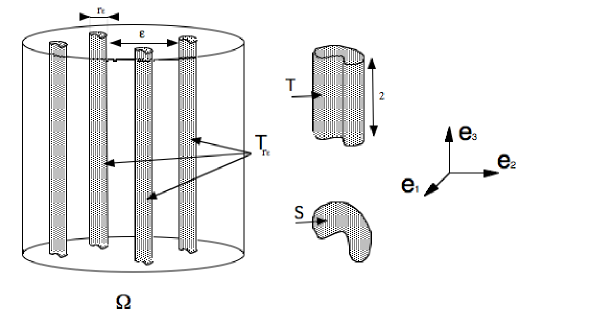
Figure 1. The fibered structure

We are concerned with the homogenization of Problem 1.1 when $f,g:\mathbb{S}^{3}\to\mathbb{R}$ are strictly convex and satisfy

$$c|\boldsymbol{M}|^{p}\leq f(\boldsymbol{M})\leq C|\boldsymbol{M}|^{p},\qquad\ c|\boldsymbol{M}|^{p}\leq g(\boldsymbol{M})\leq C|\boldsymbol{M}|^{p}\quad\forall\boldsymbol{M}\in\mathbb{S}^{3},$$ (3.5)

for some $p\in(1,+\infty)$ and some positive constants $c,C$. We prove that the limit problem depends on the parameters $k$, $\kappa$ and $\gamma^{(p)}$ defined by (1.2), (1.3). We focuse on the case

$$k>0,\qquad\quad\gamma^{(p)}>0.$$ (3.6)

Setting

$$f^{\infty,p}(\boldsymbol{M}):=\limsup_{t\to+\infty}\frac{f(t\boldsymbol{M})}{t^{p}};\quad g^{0,p}(\boldsymbol{M}):=\liminf_{t\to 0^{+}}\frac{g(t\boldsymbol{M})}{t^{p}}\qquad\forall\boldsymbol{M}\in\mathbb{S}^{3},$$ (3.7)

we suppose that

$$\left|f(\boldsymbol{M})-f^{\infty,p}(\boldsymbol{M})\right|\leq C(1+|\boldsymbol{M}|^{p-\varsigma}) \forall\boldsymbol{M}\in\mathbb{S}^{3}\quad\hskip 28.45274pt\hbox{ if }\ 1<p\leq 2,$$ (3.8)

$$\left|\frac{g(t\boldsymbol{M})}{t^{p}}-g^{0,p}(\boldsymbol{M})\right|\leq\varpi(t)|\boldsymbol{M}|^{p} \forall\boldsymbol{M}\in\mathbb{S}^{3},\ \forall t\in(0,1)\quad\hbox{ if }\kappa>0,$$

for some $\varsigma$, $\varpi$ verifying

$$\varsigma\in(0,p),\quad\varpi\in L^{\infty}(0,1),\quad\lim_{t\to 0}\varpi(t)=0.$$ (3.9)

Under these hypotheses, we show that the solution $\boldsymbol{u}_{\varepsilon}$ to (1.1) converges in a sense defined below to $\boldsymbol{u}$, the sequence $\left(\boldsymbol{v}_{\varepsilon},\theta_{\varepsilon}\right)$ given by

$$\boldsymbol{v}_{\varepsilon}(x):=\sum_{i\in I_{\varepsilon}}\left({\int\!\!\!\!\!\!-}_{S_{r_{\varepsilon}}^{i}}\boldsymbol{u}_{\varepsilon}(s,x_{3})d{\mathcal{H}}^{2}(s)\right)\mathds{1}_{Y_{\varepsilon}^{i}}(x^{\prime}),\quad\tau:=\frac{2\,{\int\!\!\!\!-}_{S}|y|^{2}dy}{{\rm diam}S},$$ (3.10)

$$\theta_{\varepsilon}(x)\hskip-2.84544pt:=\hskip-2.84544pt\sum_{i\in I_{\varepsilon}}\frac{1}{\tau}{\int\!\!\!\!\!\!-}_{{\hskip-2.84544ptS_{r_{\varepsilon}}^{i}}}\hskip-5.69046pt\left(-\frac{y_{\varepsilon 2}}{r_{\varepsilon}}u_{\varepsilon 1}+\frac{y_{\varepsilon 1}}{r_{\varepsilon}}u_{\varepsilon 2}\right)\hskip-2.84544pt(s,x_{3})d{\mathcal{H}}^{2}(s)\mathds{1}_{Y_{\varepsilon}^{i}}(x^{\prime}),$$

where

$$\boldsymbol{y}_{\varepsilon}(x^{\prime}):=\sum_{i\in I_{\varepsilon}}\left((x_{1}-\varepsilon i_{1})\boldsymbol{e}_{1}+(x_{2}-\varepsilon i_{2})\boldsymbol{e}_{2}\right)\mathds{1}_{Y_{\varepsilon}^{i}}(x^{\prime}),$$ (3.11)

converges, up to a subsequence to $(\boldsymbol{v},\theta)$, and, if $\kappa>0$, $\left(\frac{1}{r_{\varepsilon}}v_{\varepsilon 3},\frac{1}{r_{\varepsilon}}\theta_{\varepsilon}\right)$, converges up to a subsequence, to $(w,\delta)$, where the couple $(\boldsymbol{u},\boldsymbol{v}^{tuple})$ defined by (1.6) is a solution to

$$({\mathcal{P}}^{hom}):\inf_{(\boldsymbol{u},\boldsymbol{v}^{tuple})\in W^{1,p}_{b}(\Omega;\mathbb{R}^{3})\times{\mathcal{D}}}\Phi(\boldsymbol{u},\boldsymbol{v}^{tuple})-\int_{\Omega}\boldsymbol{f}.\boldsymbol{u}dx,$$ (3.12)

and $\boldsymbol{u}$ is the unique solution to

$$\inf_{\boldsymbol{u}\in W^{1,p}_{b}(\Omega;\mathbb{R}^{3})}F(\boldsymbol{u})-\int_{\Omega}\boldsymbol{f}.\boldsymbol{u}dx,\qquad\qquad F(\boldsymbol{u}):=\inf_{\boldsymbol{v}^{tuple}\in{\mathcal{D}}}\Phi(\boldsymbol{u},\boldsymbol{v}^{tuple}).$$ (3.13)

The functional $\Phi$ is defined by

$$\Phi(\boldsymbol{u},\boldsymbol{v}^{tuple}):=\int_{\Omega}f(\boldsymbol{e}(\boldsymbol{u}))+c^{f}(\boldsymbol{v}-\boldsymbol{u},\theta)+g^{hom}({\bm{\textgoth{D}}}\,\boldsymbol{v}^{tuple})dx,$$ (3.14)

where, if $\kappa=0$,

$${\bm{\textgoth{D}}}\,\boldsymbol{v}^{tuple}:=\left(\frac{\partial v_{3}}{\partial x_{3}},\frac{\partial\theta}{\partial x_{3}}\right),$$ (3.15)

$$g^{hom}\left(a,\beta\right):=\inf_{\boldsymbol{q}\in W^{1,p}(S;\mathbb{R}^{3})}k{\int\!\!\!\!\!\!-}_{S}g\left({\bm{\textgoth{L}}}\left(\boldsymbol{q},a,\beta\right)\right)dy,$$

$${\bm{\textgoth{L}}}(\boldsymbol{q},a,\beta):=\boldsymbol{e}_{y}(\boldsymbol{q})+\frac{2}{{\rm diam}S}\beta(-y_{2}\boldsymbol{e}_{1}\odot\boldsymbol{e}_{3}+y_{1}\boldsymbol{e}_{2}\odot\boldsymbol{e}_{3})+a\boldsymbol{e}_{3}\otimes\boldsymbol{e}_{3},$$

if $\kappa>0$,

$${\bm{\textgoth{D}}}\,\boldsymbol{v}^{tuple}:=\left(\frac{\partial^{2}v_{1}}{\partial x_{3}^{2}},\frac{\partial^{2}v_{2}}{\partial x_{3}^{2}},\frac{\partial w}{\partial x_{3}},\frac{\partial\delta}{\partial x_{3}}\right),$$ (3.16)

$$g^{hom}(\zeta_{1},\zeta_{2},a,\beta):=\!\!\inf_{\boldsymbol{q}\in W^{1,p}(S;\mathbb{R}^{3})}\kappa{\int\!\!\!\!\!\!-}_{S}g^{0,p}\left({\bm{\textgoth{J}}}(\boldsymbol{q},\zeta_{1},\zeta_{2},a,\beta)\right)dy,$$

$${\bm{\textgoth{J}}}(\boldsymbol{q},\zeta_{1},\zeta_{2},a,\beta):={\bm{\textgoth{L}}}(\boldsymbol{q},a,\beta)-\left(\sum_{\alpha=1}^{2}\zeta_{\alpha}y_{\alpha}\right)\boldsymbol{e}_{3}\otimes\boldsymbol{e}_{3},$$

and $c^{f}$ is defined by (1.13) in terms of ${\rm cap}^{f}$ given by (1.14), and of any sequence $(R_{\varepsilon})$ verifying

$$0<r_{\varepsilon}\ll R_{\varepsilon}\ll\varepsilon\ll 1,\quad R_{\varepsilon}\ll r_{\varepsilon}^{2-p},\quad R_{\varepsilon}\ll\frac{1}{\sqrt{|\log r_{\varepsilon}|}}\ \hbox{ if }\ p=2.$$ (3.17)

We show that $c^{f}$ is well defined, convex, independent of $(R_{\varepsilon})$ and, if $p\geq 2$, of $S$, and satisfies

$$\left.\begin{aligned} &c^{f}(\boldsymbol{a},\zeta)=\gamma^{(p)}{\rm cap}^{f^{\infty,p}}(\boldsymbol{a},\zeta\boldsymbol{e}_{3};S,\mathbb{R}^{2}),\\ &c\gamma^{(p)}(|\boldsymbol{a}|^{p}+|\zeta|^{p})\leq c^{f}(\boldsymbol{a},\zeta)\leq C\gamma^{(p)}(|\boldsymbol{a}|^{p}+|\zeta|^{p})\end{aligned}\right\} \hbox{if }1<p<2,$$ (3.18)

$$\left.\begin{aligned} &c\gamma^{(2)}|\boldsymbol{a}|^{2}\leq c^{f}(\boldsymbol{a},0)\leq C\gamma^{(2)}|\boldsymbol{a}|^{2}\\ &c^{f}(\boldsymbol{a},\zeta)=+\infty\qquad\hbox{ if }\zeta\not=0,\end{aligned}\right\} \hbox{if }\ p=2,$$

$$\ \,c^{f}(0,0)=0,\quad c^{f}(\boldsymbol{a},\zeta)=+\infty\ \ \hbox{if }\ \ (\boldsymbol{a},\zeta)\not=(0,0), \hbox{if }\ p>2.$$

The set ${\mathcal{D}}$ in (3.12) is the Banach space given by

$${\mathcal{D}}:=\Big{\{}(\boldsymbol{v},\theta)\in L^{p}(\Omega;\mathbb{R}^{3})\times L^{p}(\Omega^{\prime};W^{1,p}(0,L)),$$ (3.19)

$$\qquad v_{3}\in L^{p}(\Omega^{\prime};W^{1,p}(0,L)),v_{3}=\theta=0\text{ on }\Omega^{\prime}\times\{0\}\Big{\}}\ \hskip-91.04872pt\text{ if }0<k<+\infty,$$

$${\mathcal{D}}:=\left\{(\boldsymbol{v},\theta)\in L^{p}(\Omega;\mathbb{R}^{3})\times L^{p}(\Omega),\ v_{3}=\theta=0\right\}\ \hskip-91.04872pt\text{ if }(k,\kappa)\hskip-2.84544pt=\hskip-2.84544pt(+\infty,0),$$

$${\mathcal{D}}:=\Big{\{}\hskip-2.84544pt(\boldsymbol{v},\theta,w,\delta)\hskip-2.84544pt\in\hskip-2.84544ptL^{p}(\Omega^{\prime};W^{2,p}(0,L;\mathbb{R}^{3}))\times L^{p}(\Omega^{\prime};W^{1,p}(0,L))^{3},v_{3}\!=\!\theta\!=0,$$

$$\qquad w\!=\!\delta\!=\!v_{\alpha}=\!\frac{\partial v_{\alpha}}{\partial x_{3}}\!=0\text{ on }\Omega^{\prime}\times\{0\}\ (\alpha\in\{1,2\})\Big{\}}\qquad \hskip-91.04872pt\text{ if }0\!<\!\kappa\!<\!+\infty,$$

$${\mathcal{D}}:=\left\{0\right\}\hskip 85.35826pt \hskip-91.04872pt\text{ if }k=\kappa=+\infty.$$

Theorem 1.

Assume (3.2), (3.3), (3.5), (3.6), (3.8), then the solution $\boldsymbol{u}_{\varepsilon}$ to (1.1) weakly converges in $W_{b}^{1,p}(\Omega;\mathbb{R}^{3})$ to $\boldsymbol{u}$, the couple $(\boldsymbol{v}_{\varepsilon},\theta_{\varepsilon})$ defined by (3.10) weakly converges in $L^{p}(\Omega;\mathbb{R}^{3})\times L^{p}(\Omega)$, up to a subsequence, to $(\boldsymbol{v},\theta)$, and, if $\kappa>0$, $(\frac{1}{r_{\varepsilon}}v_{\varepsilon 3},\frac{1}{r_{\varepsilon}}\theta_{\varepsilon})$ weakly converges in $(L^{p}(\Omega))^{2}$, up to a subsequence, to $(w,\delta)$, where $(\boldsymbol{u},\boldsymbol{v}^{tuple})$ given by (1.6) is a solution to (3.12) and $\boldsymbol{u}$ is the unique solution to (3.13).

Remark 1.

(i) The functional $F$ in (3.13) is the $\Gamma$-limit of the sequence $(F_{\varepsilon})$ in the weak topology of $W_{b}^{1,p}(\Omega;\mathbb{R}^{3})$ (see Remark 11).
(ii) If $\gamma^{(p)}=0$ or $k=0$, the solution $\boldsymbol{u}_{\varepsilon}$ to (1.1) weakly converges in $W_{b}^{1,p}(\Omega;\mathbb{R}^{3})$ to the unique solution to: $\inf_{\boldsymbol{u}\in W^{1,p}_{b}(\Omega;\mathbb{R}^{3})}\int_{\Omega}f(\boldsymbol{e}(\boldsymbol{u}))dx-\int_{\Omega}\boldsymbol{f}\cdot\boldsymbol{u}dx$.
(iii) If $f^{\infty,p}$ and $g^{0,p}$ are strictly convex, which the strict convexities of $f$ and $g$ do not ensure, and $p\not=2$, then $\Phi$ is strictly convex, the solution to (3.12) unique, and all convergences stated in Theorem 1 hold for the whole sequences.
(iv) Linear isotropic elasticity. If $f=f_{\lambda_{0},\mu_{0}}$ and $g=f_{\lambda_{1},\mu_{1}}$ for some $\lambda_{0},\lambda_{1}\geq 0$, $\mu_{0},\mu_{1}>0$, where

$$f_{\lambda,\mu}(\boldsymbol{M}):=\frac{\lambda}{2}({\rm tr}\boldsymbol{M})^{2}+\mu\boldsymbol{M}:\boldsymbol{M}\quad\forall\boldsymbol{M}\in\mathbb{S}^{3},$$ (3.20)

we prove (see Remark 10) that

$$c^{f_{\lambda_{0},\mu_{0}}}(\boldsymbol{a},0)=\gamma^{(2)}\boldsymbol{a}\cdot 2\mu_{0}\pi\left(2\frac{\lambda_{0}+2\mu_{0}}{\lambda_{0}+3\mu_{0}}(\boldsymbol{e}_{1}\otimes\boldsymbol{e}_{1}+\boldsymbol{e}_{2}\otimes\boldsymbol{e}_{2})+\boldsymbol{e}_{3}\otimes\boldsymbol{e}_{3}\right)\boldsymbol{a},$$ (3.21)

and deduce from (3.15) and (3.16) that, if $\kappa=0$,

$$\Phi_{fiber}(\boldsymbol{v}^{tuple})=k\mu_{1}\int_{\Omega}\frac{3\lambda_{1}+2\mu_{1}}{2(\lambda_{1}+\mu_{1})}\left|\frac{\partial v_{3}}{\partial x_{3}}\right|^{2}+\frac{2m}{({\rm diam}S)^{2}}\left|\frac{\partial\theta}{\partial x_{3}}\right|^{2}dx,$$ (3.22)

and, if $\kappa>0$,

$$\Phi_{fiber}(\boldsymbol{v}^{tuple})=\kappa\mu_{1}\int_{\Omega}\frac{3\lambda_{1}+2\mu_{1}}{2(\lambda_{1}+\mu_{1})}\Bigg{[}\sum_{\alpha=1}^{2}\left({\int\!\!\!\!\!\!-}_{S}y_{\alpha}^{2}dy\right)\left|\frac{\partial^{2}v_{\alpha}}{\partial x_{3}^{2}}\right|^{2}$$ (3.23)

$$\qquad\qquad-2\left({\int\!\!\!\!\!\!-}_{S}y_{1}y_{2}dy\right)\frac{\partial^{2}v_{1}}{\partial x_{3}^{2}}\frac{\partial^{2}v_{2}}{\partial x_{3}^{2}}+\left|\frac{\partial w}{\partial x_{3}}\right|^{2}\Bigg{]}+\frac{2m}{({\rm diam}S)^{2}}\left|\frac{\partial\delta}{\partial x_{3}}\right|^{2}dx,$$

where $m:=\inf_{\varphi\in H^{1}(S)}{\int\!\!\!\!\!\!-}_{S}\left(\tfrac{\partial\varphi}{\partial y_{1}}-y_{2}\right)^{2}+\left(\tfrac{\partial\varphi}{\partial y_{2}}+y_{1}\right)^{2}dy$. This infimum being attained, it results from the Schwarz theorem that $m>0$. Noticing that, by (3.23), the infimum (3.12) is achieved by $(w,\delta)=(0,0)$ and that, by (3.18), $\theta=0$, we recover the formulae obtained for $S=D$ in [15, Remark 2.2].
(v) The following example shows that $\delta$ doesn’t vanish, in general, when anisotropic fibers are considered: assume that $0<\kappa<+\infty$ and

$$g(\boldsymbol{M}):=\sum_{\alpha,\beta=1}^{2}M_{\alpha\beta}M_{\alpha\beta}+M_{13}^{2}+M_{33}^{2}+M_{13}M_{33}+M_{23}^{2}.$$

Then, a solution to the minimization problem (3.16) is $\boldsymbol{q}:=(\zeta_{1}\varphi^{(1)}+\zeta_{2}\varphi^{(2)}+a\varphi^{(3)}+\tilde{\beta}\varphi^{(4)})\boldsymbol{e}_{3}$, where $\tilde{\beta}:=\tfrac{1}{{\rm diam}S}\beta$ and $\varphi^{(1)},..,\varphi^{(4)}$ are solutions in $H^{1}(S)/\mathbb{R}$ to the Neumann problems ($\boldsymbol{n}$: outer unit normal to $\partial S$)

$$({\mathcal{P}}^{(1)}):\Delta\varphi^{(1)}=1\quad\hbox{ in }S,\quad \boldsymbol{\nabla}\varphi^{(1)}\cdot\boldsymbol{n}=y_{1}n_{1}\quad\quad \hbox{ on }\partial S,$$

$$({\mathcal{P}}^{(2)}):\Delta\varphi^{(2)}=0\quad\hbox{ in }S,\quad \boldsymbol{\nabla}\varphi^{(2)}\cdot\boldsymbol{n}=y_{2}n_{2}\quad\quad \hbox{ on }\partial S,$$

$$({\mathcal{P}}^{(3)}):\Delta\varphi^{(3)}=0\quad\hbox{ in }S,\quad \boldsymbol{\nabla}\varphi^{(3)}\cdot\boldsymbol{n}=-n_{1}\quad\quad \hbox{ on }\partial S,$$

$$({\mathcal{P}}^{(4)}):\Delta\varphi^{(4)}=0\quad\hbox{ in }S,\quad \boldsymbol{\nabla}\varphi^{(4)}\cdot\boldsymbol{n}=-2\begin{pmatrix}-y_{2}\\ y_{1}\end{pmatrix}\cdot\boldsymbol{n} \hbox{ on }\partial S,$$

respectively. We deduce that $g^{hom}(\zeta_{1},\zeta_{2},a,\beta)$ $=\begin{pmatrix}\zeta_{1}\\ \zeta_{2}\\ a\\ \tilde{\beta}\end{pmatrix}\cdot\boldsymbol{C}\begin{pmatrix}\zeta_{1}\\ \zeta_{2}\\ a\\ \tilde{\beta}\end{pmatrix}$, where

$$\boldsymbol{C}\in\mathbb{S}^{4},\quad C_{33}=\kappa,\quad C_{44}=\kappa{\int\!\!\!\!\!\!-}_{S}|y|^{2}dy,\quad 2C_{34}=\kappa{\int\!\!\!\!\!\!-}_{S}\tfrac{1}{2}\tfrac{\partial\varphi^{(4)}}{\partial y_{1}}dy$$

$$2C_{\alpha 3}=\kappa{\int\!\!\!\!\!\!-}_{S}\tfrac{1}{2}\tfrac{\partial\varphi^{(\alpha)}}{\partial y_{1}}dy,\quad 2C_{\alpha 4}=\kappa{\int\!\!\!\!\!\!-}_{S}-y_{\alpha}\left(\tfrac{1}{2}\tfrac{\partial\varphi^{(4)}}{\partial y_{1}}-y_{2}\right)dy\quad\forall\alpha\in\{1,2\}.$$

If $(\boldsymbol{u},\boldsymbol{v}^{tuple})$ is a solution to (3.12), then $(w,\delta)$ is a solution to $\inf_{(w,\delta)}\Phi(\boldsymbol{u},\boldsymbol{v},0,w,\delta)$. We infer

$$\begin{pmatrix}C_{33}&C_{34}\\ C_{34}&C_{44}\end{pmatrix}\begin{pmatrix}w\\ \tfrac{1}{{\rm diam}S}\delta\end{pmatrix}=\sum_{\alpha=1}^{2}\begin{pmatrix}-C_{\alpha 3}\frac{\partial v_{\alpha}}{\partial x_{3}}\\ -C_{\alpha 4}\frac{\partial v_{\alpha}}{\partial x_{3}}\end{pmatrix}.$$

If $S=D$, we obtain $\varphi^{(4)}=0$, $C_{14}=C_{34}=0$, $C_{44}=4C_{24}>0$, and deduce $\delta=-\tfrac{{\rm diam}S}{2}\tfrac{\partial v_{2}}{\partial x_{3}}$.

3.2. Problem 1.16

Assuming

$$r_{\varepsilon}=\varepsilon,\quad\overline{S}\subset\ring{Y},$$ (3.24)

and

$$|{\boldsymbol{\varphi}}|_{L^{p}(\Omega;\mathbb{R}^{3})}\leq CF^{soft}_{\varepsilon}({\boldsymbol{\varphi}})\quad\forall{\boldsymbol{\varphi}}\in W^{1,p}_{b}(\Omega;\mathbb{R}^{3}),$$ (3.25)

we prove that the effective problem associated to (1.16) is

$$\inf_{(\boldsymbol{u},\boldsymbol{v}^{tuple})\in L^{p}(\Omega;\mathbb{R}^{3})\times{\mathcal{D}}}\quad\Phi^{soft}(\boldsymbol{u},\boldsymbol{v}^{tuple})-\int_{\Omega}\boldsymbol{f}\cdot\boldsymbol{u},$$ (3.26)

$$\Phi^{soft}(\boldsymbol{u},\boldsymbol{v}^{tuple})=\int_{\Omega}c^{f}_{soft}(\boldsymbol{v}-\boldsymbol{u},\theta)dx+\int_{\Omega}g^{hom}({\bm{\textgoth{D}}}\,\boldsymbol{v}^{tuple})dx,$$

where $c^{f}_{soft}$, $g^{hom}$ and ${\mathcal{D}}$ are defined by (1.17), (3.15), (3.16) and (3.19), respectively.

Theorem 2.

Assume (3.24) and (3.25), then the solution $\boldsymbol{u}_{\varepsilon}$ to (1.16) weakly converges in $L^{p}(\Omega;\mathbb{R}^{3})$, up to a subsequence, to $\boldsymbol{u}$, and the convergences of $(\boldsymbol{v}_{\varepsilon},\theta_{\varepsilon})$ and $(\frac{1}{\varepsilon}v_{\varepsilon 3},\frac{1}{\varepsilon}\theta_{\varepsilon})$ stated in Theorem 1 hold, where $(\boldsymbol{u},\boldsymbol{v}^{tuple})$ is a solution to (3.26).

Remark 2.

(i) Theorems 1 and 2 can be generalized to multiphase media comprising non-intersecting families of parallel fibers distributed in different directions (for Theorem 2, case $p=2$, see [7, Sec. 4]).

(ii) The condition (3.25) is guaranteed when $\kappa>0$ or when suitable multiphase media described in [7, Sec. 5] are considered, for instance when $k>0$ and the fibers are distributed in at least three independent directions.

(iii) Most of Remark 1 applies to Problem 1.16.

4. Variants

4.1. Non-periodic case

The study of Problem 1.1 can be extended to a non-periodic setting: we then parametrize it by the size $r$ of the cross-sections of the fibers. The collection of fibers is described in terms of the image $G_{r}$ of the set of their principal axes under the orthogonal projection onto $\Omega^{\prime}$, by setting

$$T_{r}(G_{r}):=\bigcup_{t\in G_{r}}(t+rS)\times(0,L).$$ (4.1)

We assume that $(G_{r})_{r>0}$ is a family of finite subsets of $\Omega^{\prime}$ satisfying, as $r\to 0$,

$$r\ll\inf_{t_{1},t_{2}\in G_{r},t_{1}\not=t_{2}}|t_{1}-t_{2}|\ll 1;\qquad r\ll{\rm dist}(G_{r},\partial\Omega^{\prime}).$$ (4.2)

We focuse on the case $p\in(1,2]$. To take advantage of the notations introduced in the periodic case, we fix an arbitrary positive real number $\gamma^{(p)}$ and introduce the small parameter $\varepsilon_{r}$ defined by

$$\varepsilon_{r}:=\frac{r^{\frac{2-p}{2}}}{\left(\gamma^{(p)}\right)^{1/2}}\quad\hbox{if }\ p\in(1,2);\qquad\varepsilon_{r}:=\frac{1}{\sqrt{\gamma^{(2)}|\log{r}|}}\quad\hbox{if }\ p=2.$$ (4.3)

By (1.3) we have $\gamma_{\varepsilon_{r}}^{(p)}(r)=\gamma^{(p)}$ for every $r>0$. Given a sequence of positive real numbers $(l_{\varepsilon_{r}})_{r>0}$, we consider the sequence of problems $({\mathcal{P}}_{r}(G_{r}))_{r>0}$ formally deduced from (1.1) by substituting $T_{r}(G_{r})$ for $T_{r_{\varepsilon}}$ and $l_{\varepsilon_{r}}$ for $l_{\varepsilon}$. The function defined by

$$n_{G_{r}}(x^{\prime}):=\sum_{i\in I_{\varepsilon_{r}}}\sharp\left(G_{r}\cap Y_{\varepsilon_{r}}^{i}\right)\ \mathds{1}_{Y_{\varepsilon_{r}}^{i}}(x^{\prime})\qquad\forall x^{\prime}\in\Omega^{\prime},$$ (4.4)

where $I_{\varepsilon_{r}}$ and $Y_{\varepsilon_{r}}^{i}$ are given by (3.3), locally approximates to the number of fibers crossing a square of size $\varepsilon_{r}$ in the cross-section of $\Omega$. We suppose that $(n_{G_{r}})_{r>0}$ is bounded in $L^{\infty}(\Omega^{\prime})$ and weakly^⋆ converges to some $n$ as $r\to 0$. Setting $\mu:=n{\mathcal{L}}^{2}_{\lfloor\overline{\Omega}^{\prime}}$, by combining the argument of the proof of Theorem 1 with the one developed in [16], one can prove that the effective problem takes the form

$$({\mathcal{P}}^{hom,\,\mu}):\inf_{\boldsymbol{u}\in W^{1,p}_{b}(\Omega)}F^{\mu}(\boldsymbol{u})-\int_{\Omega}\boldsymbol{f}.\boldsymbol{u}dx;\quad F^{\mu}(\boldsymbol{u}):=\hskip-8.5359pt\inf_{\boldsymbol{v}^{tuple}\in{\mathcal{D}}^{\mu}}\Phi^{\mu}(\boldsymbol{u},\boldsymbol{v}^{tuple}),$$ (4.5)

$$\Phi^{\mu}(\boldsymbol{u},\boldsymbol{v}^{tuple})=\int_{\Omega}f(\boldsymbol{e}(\boldsymbol{u}))dx+\int_{\Omega}c^{f}(\boldsymbol{v}-\boldsymbol{u},\theta)+g^{hom}({\bm{\textgoth{D}}}\,\boldsymbol{v}^{tuple})d\mu\otimes{\mathcal{L}}^{1}\hskip-4.26773pt,$$

where $c^{f}$ and $g^{hom}$ are given by (3.15), (3.16) and (3.18) in terms of $\gamma^{(p)}$ introduced above and $k$, $\kappa$ defined by substituting $\varepsilon_{r}$ for $\varepsilon$ in (1.2). The domain ${\mathcal{D}}^{\mu}$ is deduced from (3.19) by substituting $L^{p}_{\mu\otimes{\mathcal{L}}^{1}}(\Omega;\mathbb{R}^{3})$ for $L^{p}(\Omega;\mathbb{R}^{3})$, the spaces $L^{p}_{\mu}(\Omega^{\prime};E)$ for $L^{p}(\Omega^{\prime};E)$ for any Banach space $E$, and by replacing the homogeneous Dirichlet conditions on $\Omega^{\prime}\times\{0\}$ by homogeneous Dirichlet conditions $\mu\otimes\delta_{\{0\}}$-a.e. on $\Omega^{\prime}\times\{0\}$.

Theorem 3.

Under the assumptions stated above, the solution $\boldsymbol{u}_{r}$ to $({\mathcal{P}}_{r}(G_{r}))$ weakly converges in $W^{1,p}_{b}(\Omega;\mathbb{R}^{3})$ as $r\to 0$ to the unique solution $\boldsymbol{u}$ to (4.5).

Remark 3.

(i) Under the same assumptions, one can show that the measure $\tilde{m}_{r}$, defined by substituting $T_{r}(G_{r})$ for $S_{r_{\varepsilon}}\times(0,L)$ and $(r,\varepsilon_{r})$ for $(r_{\varepsilon},\varepsilon)$ in (5.9), weakly^⋆ converges to $\mu\otimes{\mathcal{L}}^{1}$ in ${\mathcal{M}}(\overline{\Omega})$, and the sequences $(\tilde{\boldsymbol{v}}_{r}\tilde{m}_{r})$, $(\tilde{\theta}_{r}\tilde{m}_{r})$ and, if $\kappa>0$, $\left(\tfrac{1}{\varepsilon_{r}}\tilde{v}_{r3}\tilde{m}_{r}\right)$ and $\left(\tfrac{1}{\varepsilon_{r}}\tilde{\theta}_{r}\tilde{m}_{r}\right)$, where

$$\tilde{\boldsymbol{v}}_{r}(x):=\sum_{t\in G_{r}}\left({\int\!\!\!\!\!\!-}_{{t+rS}}\boldsymbol{u}_{r}(s,x_{3})d{\mathcal{H}}^{2}(s)\right)\mathds{1}_{t+rS}(x^{\prime}),$$

$$\tilde{\theta}_{r}(x):=\sum_{t\in G_{r}}\frac{1}{\tau}{\int\!\!\!\!\!\!-}_{t+rS}\hskip-5.69046pt\left(-\frac{\tilde{y}_{r2}}{r}u_{r1}+\frac{\tilde{y}_{r1}}{r}u_{r2}\right)\hskip-2.84544pt(s,x_{3})d{\mathcal{H}}^{2}(s)\mathds{1}_{t+rS}(x^{\prime}),$$

$$\tilde{\boldsymbol{y}}_{r}(x^{\prime}):=\sum_{t\in G_{r}}\left((x_{1}-t_{1})\boldsymbol{e}_{1}+(x_{2}-t_{2})\boldsymbol{e}_{2}\right)\mathds{1}_{t+rS}(x^{\prime}),$$

weakly^⋆ converge up to a subsequence in ${\mathcal{M}}(\overline{\Omega};\mathbb{R}^{3})$ and ${\mathcal{M}}(\overline{\Omega})$ to $\boldsymbol{v}\mu\otimes{\mathcal{L}}^{1}$, $\theta\mu\otimes{\mathcal{L}}^{1}$, $w\mu\otimes{\mathcal{L}}^{1}$, and $\delta\mu\otimes{\mathcal{L}}^{1}$, respectively, where $\boldsymbol{v}^{tuple}$, defined by (1.6), is a solution to the minimization problem defining $F^{\mu}(\boldsymbol{u})$ in (4.5).
(ii) Theorem 3 holds, in some cases, when $(n_{G_{r}}{\mathcal{L}}^{2}_{\lfloor\Omega^{\prime}})$ is bounded in ${\mathcal{M}}(\overline{\Omega}^{\prime})$ and weakly^⋆ converges to some singular measure $\mu$ which vanishes on all Borel subset of $\overline{\Omega}^{\prime}$ of $p$-capacity zero. For instance, assume that $\Omega^{\prime}=(0,L)^{2}$ and set

$$G_{r}:=\left\{(L/2,\varepsilon_{r}^{2}i),\ i\in\mathbb{Z}\right\}\cap\ \{L/2\}\times(\varepsilon_{r}^{2},L-\varepsilon_{r}^{2}).$$

The set $T_{r}(G_{r})$ defined by (4.1) represents a family of fibers whose principal axes are $\varepsilon_{r}^{2}$-periodically distributed on the surface $\Sigma:=\{L/2\}\times(0,L)^{2}$. The sequence $(n_{G_{r}}{\mathcal{L}}^{2}_{\lfloor{\Omega^{\prime}}})$ defined by (4.4) is bounded in ${\mathcal{M}}(\overline{\Omega}^{\prime})$ and weakly^⋆ converges to $\mu:={\mathcal{H}}^{1}_{\lfloor\{L/2\}\times(0,L)}$. One can show, by combining the argument of the proof of Theorem 1 with that developed in [14], that Theorem 3 holds, as well as the convergences stated in (i).
(iii) Dirichlet problems in varying domains. Under the assumptions of Theorems 1 or 3 (or Remark 3 (ii)), the solution to

$$\inf_{\boldsymbol{u}_{r}\in W^{1,p}_{b}(\Omega;\mathbb{R}^{3})}\left\{\int_{\Omega}f(\boldsymbol{e}(\boldsymbol{u}_{r}))dx-\int_{\Omega}\boldsymbol{f}.\boldsymbol{u}_{r}dx,\quad\boldsymbol{u}_{r}=0\hbox{ in }\ T_{r}(G_{r})\right\},$$ (4.6)

weakly converges in $W^{1,p}_{b}(\Omega;\mathbb{R}^{3})$ to the unique solution to

$$\inf_{\boldsymbol{u}\in W^{1,p}_{b}(\Omega;\mathbb{R}^{3})}\int_{\Omega}f(\boldsymbol{e}(\boldsymbol{u}))dx+\int_{\Omega}c^{f}(\boldsymbol{u},0)d\mu\otimes{\mathcal{L}}^{1}-\int_{\Omega}\boldsymbol{f}.\boldsymbol{u}dx,$$ (4.7)

deduced from $({\mathcal{P}}^{hom,\,\mu})$ by substituting $0$ for $\boldsymbol{v}^{tuple}$. The second term is analogous to the so-called ”strange term” [30, 43]. If $(n_{G_{r}})_{r>0}$ is only assumed to be bounded in $L^{1}(\Omega^{\prime})$ and to weakly^⋆ converge to some arbitrary measure $\mu$, we expect the limit problem associated with (4.6) to depend, not on $\mu$, but, up to a subsequence, on some measure $\mu_{0}$ defined through a variant of the $\gamma$-convergence introduced in [34]. Many references on this subject can be found in [35]. In particular, compactness results ensuring the existence of a $\gamma$-converging subsequence have been established in various contexts. Under (4.2), the limit problem associated with (4.6) is likely to be deduced from (4.7), formally, by substituting such a measure $\mu_{0}$ for $\mu$. This suggests that the limit problem associated with $({\mathcal{P}}_{r}(G_{r}))$ might possibly be $({\mathcal{P}}^{hom,\,\mu_{0}})$.

(iv) The assumption (4.3) on the choice of $\varepsilon_{r}$ was omitted in [16]. In order the results stated in [16] to be correct, one should either assume in [16, (17)] that $\gamma^{(p)}$ is finite (hence $1<p\leq 2$), or in [16, (5)] that $n_{\varepsilon}$ is bounded from below by a positive constant, otherwise the asymptotic behavior of the sequence $(\gamma_{\varepsilon}(r)n_{\varepsilon})$, whose knowledge is necessary to obtain for instance [16, (126)], would be undetermined.

4.2. Random case

Assuming $1<p\leq 2$, fixing $d>0$, we set

$${{\mathfrak{O}}}:=\Big{\{}\omega\in 2^{\mathbb{R}^{2}},\ \forall(\omega_{1},\omega_{2})\in\omega^{2},\ \omega_{1}\not=\omega_{2}\ \Rightarrow\ |\omega_{1}-\omega_{2}|\geq d\Big{\}}.$$ (4.8)

One can check that the finite metric $d_{{\mathfrak{O}}}:(\omega,\omega^{\prime})\in{{\mathfrak{O}}}^{2}\to\inf\{1,d_{\mathcal{H}}(\omega,\omega^{\prime})\}$, where $d_{\mathcal{H}}$ stands for the Hausdorff distance, turns ${{\mathfrak{O}}}$ into a complete metric space. Denoting by ${\mathcal{B}}({{\mathfrak{O}}})$ the associated Borel $\sigma$-algebra on ${{\mathfrak{O}}}$, we consider a probability measure $P$ on $({{\mathfrak{O}}},{\mathcal{B}}({{\mathfrak{O}}}))$ satisfying

$$P(A+z)=P(A)\quad\forall\ z\in\mathbb{Z}^{2},\quad\forall\,A\in{\mathcal{B}}({{\mathfrak{O}}}).$$

We introduce the $\sigma$-algebra ${\mathcal{F}}$ and the random variable $n_{0}$ on ${{\mathfrak{O}}}$ defined by

$${\mathcal{F}}:=\left\{A\in{\mathcal{B}}({{\mathfrak{O}}}),\ A+z=A\quad\forall z\in\mathbb{Z}^{2}\right\},\qquad n_{0}(\omega):=\sharp\left(\omega\cap\left[-\frac{1}{2},\frac{1}{2}\right[^{2}\right).$$

We denote by ${E}_{{P}}^{{\mathcal{F}}}n_{0}$ the conditional expectation of $n_{0}$ given ${\mathcal{F}}$ w.r.t. ${P}$. We fix a positive real number $\gamma^{(p)}$ and set

$$G_{r}(\omega):=\varepsilon_{r}\omega\cap\{x\in\Omega^{\prime},\ {\rm dist}(x,\partial\Omega^{\prime})\geq\varepsilon_{r}\}\qquad\forall r>0,\ \forall\omega\in{{\mathfrak{O}}},$$

where $\varepsilon_{r}$ is given by (4.3). The following statement is proved in [10, Th. 2.4.2]:

Theorem 4.

Under the assumptions stated above, there exists a sequence $(r_{k})_{k\in\mathbb{N}}$ converging to $0$ and a $P$-negligible set ${{\mathfrak{N}}}\in{\mathcal{B}}({{\mathfrak{O}}})$ such that, for each $\omega\in{{\mathfrak{O}}}\setminus{{\mathfrak{N}}}$, the sequence $(n_{G_{r_{k}}(\omega)})$ defined by (4.4) weakly^⋆ converges in $L^{\infty}(\Omega^{\prime})$ to the constant function ${E}_{{P}}^{{\mathcal{F}}}n_{0}(\omega)$.

The assumptions (4.3) and (4.8) ensure that $G_{r}(\omega)$ satisfies (4.2). By combining Theorems 3 and 4, we obtain:

Corollary 1.

There exists a sequence $(\!r_{k}\!)_{k\in\mathbb{N}}$ converging to $0$ and a $P\!$-negligible set ${{\mathfrak{N}}}\in{\mathcal{B}}({{\mathfrak{O}}})$ such that, for all $\omega\in{{\mathfrak{O}}}\setminus{{\mathfrak{N}}}$, the solution $\boldsymbol{u}_{r_{k}}(\omega)$ to the problem $({\mathcal{P}}_{r_{k}}(G_{r_{k}}(\omega)))$ considered in Section 4.1 weakly converges in $W^{1,p}_{b}(\Omega;\mathbb{R}^{3})$ to the unique solution $\boldsymbol{u}(\omega)$ to $({\mathcal{P}}^{hom,\ \mu(\omega)})$ defined by (4.5), where $\mu(\omega):={E}_{{P}}^{{\mathcal{F}}}n_{0}(\omega){\mathcal{L}}^{2}_{\lfloor\Omega^{\prime}}$.

4.3. Large applied body forces

We consider the problems

$$\inf_{\boldsymbol{u}_{\varepsilon}\in W^{1,p}_{b}(\Omega;\mathbb{R}^{3})}F_{\varepsilon}(\boldsymbol{u}_{\varepsilon})-\int_{\Omega}\boldsymbol{f}_{\varepsilon}\cdot\boldsymbol{u}_{\varepsilon}dx,$$ (4.9)

$$\inf_{\boldsymbol{u}_{\varepsilon}\in W^{1,p}_{b}(\Omega;\mathbb{R}^{3})}F^{soft}_{\varepsilon}(\boldsymbol{u}_{\varepsilon})-\int_{\Omega}\boldsymbol{f}_{\varepsilon}\cdot\boldsymbol{u}_{\varepsilon}dx,$$ (4.10)

where, given $\boldsymbol{f}\in L^{p^{\prime}}(\Omega;\mathbb{R}^{3})$, $\boldsymbol{g}_{0}\in C(\overline{\Omega\times S};\mathbb{R}^{3})$ and $a_{0},\beta_{0}\in C(\overline{\Omega\times S})$, $\boldsymbol{f}_{\varepsilon}$ is defined in terms of $y_{\varepsilon}$ given by (3.11), by

$$\boldsymbol{f}_{\varepsilon}(x)=\boldsymbol{f}(x)+\frac{|\Omega|}{|{T_{r_{\varepsilon}}}|}\boldsymbol{g}_{0}\left(x,\frac{y_{\varepsilon}(x^{\prime})}{r_{\varepsilon}}\right)\mathds{1}_{{T_{r_{\varepsilon}}}}(x)\hskip 45.52458pt \hbox{ if }\ \kappa=0,$$ (4.11)

$$\boldsymbol{f}_{\varepsilon}(x)\hskip-1.42271pt:=\hskip-1.42271pt\boldsymbol{f}(x)+\frac{|\Omega|}{|{T_{r_{\varepsilon}}}|}\boldsymbol{g}_{0}\left(\hskip-1.42271ptx,\frac{y_{\varepsilon}(x^{\prime})}{r_{\varepsilon}}\right)\hskip-1.42271pt\mathds{1}_{{T_{r_{\varepsilon}}}}(x)+\frac{1}{r_{\varepsilon}}\frac{|\Omega|}{|{T_{r_{\varepsilon}}}|}\boldsymbol{h}_{\varepsilon}(x)\ \hbox{ if }\ 0<\kappa<+\infty,$$

with

$$\boldsymbol{h}_{\varepsilon}(x)\hskip-2.84544pt:=\hskip-2.84544pt\sum_{i\in I_{\varepsilon}}\hskip-2.84544pt\begin{pmatrix}\hskip-2.84544pt-\frac{y_{\varepsilon 2}(x^{\prime})}{r_{\varepsilon}}\beta_{0}\left(x,\frac{y_{\varepsilon}(x^{\prime})}{r_{\varepsilon}}\right)+{\int\!\!\!\!-}_{S_{r_{\varepsilon}}^{i}}\frac{y_{\varepsilon 2}(s)}{r_{\varepsilon}}\beta_{0}\left(s,x_{3},\frac{y_{\varepsilon}(s)}{r_{\varepsilon}}\right)ds\\ \hskip-2.84544pt\frac{y_{\varepsilon 1}(x^{\prime})}{r_{\varepsilon}}\beta_{0}\left(x,\frac{y_{\varepsilon}(x^{\prime})}{r_{\varepsilon}}\right)-{\int\!\!\!\!-}_{S_{r_{\varepsilon}}^{i}}\frac{y_{\varepsilon 1}(s)}{r_{\varepsilon}}\beta_{0}\left(s,x_{3},\frac{y_{\varepsilon}(s)}{r_{\varepsilon}}\right)ds\\ \hskip-2.84544pta_{0}\left(x,\frac{y_{\varepsilon}(x^{\prime})}{r_{\varepsilon}}\right)\end{pmatrix}\hskip-1.42271pt\mathds{1}_{{T_{r_{\varepsilon}}^{i}}}\hskip-2.84544pt(x).$$

We establish that the limit problems associated to (4.9) and (4.10) are

$$\inf_{(\boldsymbol{u},\boldsymbol{v}^{tuple})\in W^{1,p}_{b}(\Omega;\mathbb{R}^{3})\times{\mathcal{D}}}\Phi(\boldsymbol{u},\boldsymbol{v}^{tuple})-\int_{\Omega}\boldsymbol{f}\cdot\boldsymbol{u}dx-L(\boldsymbol{v}^{tuple}),$$ (4.12)

$$\inf_{(\boldsymbol{u},\boldsymbol{v}^{tuple})\in L^{p}(\Omega;\mathbb{R}^{3})\times{\mathcal{D}}}\Phi^{soft}(\boldsymbol{u},\boldsymbol{v}^{tuple})-\int_{\Omega}\boldsymbol{f}\cdot\boldsymbol{u}dx-L(\boldsymbol{v}^{tuple}),$$ (4.13)

respectively, where, if $\kappa=0$,

$$L(\boldsymbol{v}^{tuple})=\int_{\Omega}\left({\int\!\!\!\!\!\!-}_{S}\hskip-2.84544pt\boldsymbol{g}_{0}(x,y)dy\right)\hskip-2.84544pt\cdot\hskip-1.42271pt\boldsymbol{v}+\left({\int\!\!\!\!\!\!-}_{S}\boldsymbol{g}_{0}(x,y)\hskip-1.42271pt\cdot\hskip-1.42271pt\frac{2}{{\rm diam}S}\boldsymbol{e}_{3}\wedge\boldsymbol{y}dy\!\right)\hskip-1.42271pt\theta dx,$$ (4.14)

and, if $0<\kappa<+\infty$,

$$L(\boldsymbol{v}^{tuple})\hskip-2.84544pt=\hskip-2.84544pt\int_{\Omega}\hskip-1.42271pt\left({\int\!\!\!\!\!\!-}_{S}\hskip-2.84544pt\boldsymbol{g}_{0}(x,y)dy\right)\hskip-2.84544pt\cdot\boldsymbol{v}+\tau\left({\int\!\!\!\!\!\!-}_{S}\hskip-2.84544pt\beta_{0}(x,y)dy\right)\delta(x)$$ (4.15)

$$\hskip 56.9055pt+\left({\int\!\!\!\!\!\!-}_{S}\left(w(x)-\sum_{\alpha=1}^{2}\frac{\partial v_{\alpha}}{\partial x_{3}}(x)y_{\alpha}\right)a_{0}(x,y)dy\right)dx,$$

being $\tau$ given by (3.10).

Theorem 5.

The statements deduced from Theorems 1 and 2 by substituting (4.9), (4.12) for (1.1), (3.12) and (4.10), (4.13) for (1.16), (3.26) hold.

Remark 4.

When $\kappa>0$ and $\Phi_{fibers}$ is given by (3.23), if $(\boldsymbol{u},\boldsymbol{v}^{tuple})$ is a solution to (4.12) or (4.13), then

$$\delta(x)=\frac{\tau({\rm diam}S)^{2}}{\kappa\mu_{1}m}\left({\int\!\!\!\!\!\!-}_{S}\beta_{0}(x^{\prime},L,y)dy\right)\left(-\frac{x_{3}^{2}}{2}+L\right),$$ (4.16)

$$w(x)=\frac{l+1}{\kappa\mu_{1}(3l+2)}\left({\int\!\!\!\!\!\!-}_{S}a_{0}(x^{\prime},L,y)dy\right)\left(-\frac{x_{3}^{2}}{2}+L\right).\$$

5. Preliminary results and a priori estimates

This section is devoted to the study of the asymptotic behaviors of a sequence $(\boldsymbol{u}_{\varepsilon})$ satisfying

$$\sup_{\varepsilon>0}F_{\varepsilon}(\boldsymbol{u}_{\varepsilon})<+\infty,$$ (5.1)

and of the auxiliary sequences $(\boldsymbol{v}_{\varepsilon})$, $(\theta_{\varepsilon})$, $\left(\frac{v_{\varepsilon 3}}{r_{\varepsilon}}\right)$, $\left(\frac{\theta_{\varepsilon}}{r_{\varepsilon}}\right)$ defined by (3.10). Our main results, stated in Section 5.5, will be deduced from a series of inequalities proved in Section 5.4.

5.1. Auxiliary sequences

The proof of Theorem 1 rests on a choice of sequences of auxiliary fields

• weakly differentiable w.r.t. $x_{3}$,

• weakly relatively compact in $L^{p}$,

• locally characterizing a rigid motion approximating to the velocity in the fibers.

The selection of surface integrals in (3.10) is required to ensure the first condition, and is a hindrance to the third. To circumvent this difficulty, we introduce another couple of auxiliary sequences constructed from volume instead of surface integrals, satisfying the second and third conditions and having the same cluster points as $\boldsymbol{v}_{\varepsilon}$, $\theta_{\varepsilon}$. For convenience, we rewrite (3.10) as follows

$$\boldsymbol{v}_{\varepsilon}=\overline{{\textswab{\boldsymbol{v}}}}_{\varepsilon}^{S}(\boldsymbol{u}_{\varepsilon}),\qquad\theta_{\varepsilon}=\overline{\theta}_{\varepsilon}^{S}(\boldsymbol{u}_{\varepsilon}),$$ (5.2)

where, for any Lipschitz domain $A$ of $\mathbb{R}^{2}$ verifying

$$D\subset A\subset S,\qquad\boldsymbol{y}_{A}=0,$$ (5.3)

$\overline{{\textswab{\boldsymbol{v}}}}_{\varepsilon}^{A}$ and $\overline{\theta}_{\varepsilon}^{A}$ are the linear operators defined on $L^{p}(\Omega;\mathbb{R}^{3})$ by (see (3.3), (3.4), (3.11)):

$$\overline{{\textswab{\boldsymbol{v}}}}^{A}_{\varepsilon}({\boldsymbol{\varphi}})(x):=\sum_{i\in I_{\varepsilon}}\left({\int\!\!\!\!\!\!-}_{{A_{r_{\varepsilon}}^{i}}}{\boldsymbol{\varphi}}(s,x_{3})d{\mathcal{H}}^{2}(s)\right)\mathds{1}_{Y_{\varepsilon}^{i}}(x^{\prime}),$$ (5.4)

$$\overline{\theta}^{A}_{\varepsilon}({\boldsymbol{\varphi}})(x):=\sum_{i\in I_{\varepsilon}}\frac{{\rm diam}S}{2{\int\!\!\!\!-}_{A}|\boldsymbol{y}|^{2}dy}{\int\!\!\!\!\!\!-}_{{A_{r_{\varepsilon}}^{i}}}\hskip-8.5359pt\left(-\frac{y_{\varepsilon 2}}{r_{\varepsilon}}\varphi_{1}+\frac{y_{\varepsilon 1}}{r_{\varepsilon}}\varphi_{2}\right)(s,x_{3})d{\mathcal{H}}^{2}(s)\ \mathds{1}_{Y_{\varepsilon}^{i}}(x^{\prime}),$$

$$\overline{{\textswab{\boldsymbol{r}}}}_{\varepsilon}^{A}({\boldsymbol{\varphi}})(x):=\overline{{\textswab{\boldsymbol{v}}}}_{\varepsilon}^{A}({\boldsymbol{\varphi}})(x)+\frac{2}{{\rm diam}S}\overline{\theta}_{\varepsilon}^{A}({\boldsymbol{\varphi}})(x)\boldsymbol{e}_{3}\wedge\frac{\boldsymbol{y}_{\varepsilon}(x^{\prime})}{r_{\varepsilon}}.$$

The ”volumic” couterparts ${{\textswab{\boldsymbol{v}}}}_{\varepsilon}(\boldsymbol{u}_{\varepsilon})$ and $\theta_{\varepsilon}(\boldsymbol{u}_{\varepsilon})$ of (3.10) will be defined by splitting each fiber $T^{i}_{r_{\varepsilon}}$ into small cylinders $T_{r_{\varepsilon}}^{ij}$ of size $r_{\varepsilon}$ given by (see fig. 2)

$$T_{r_{\varepsilon}}^{ij}:=S_{r_{\varepsilon}}^{i}\hskip-2.84544pt\times\Delta_{r_{\varepsilon}}^{j},\quad\Delta_{r_{\varepsilon}}^{j}:=r_{\varepsilon}\left(2j+\left(0,2\right]\right)\hskip-1.42271pt,\quad L_{\varepsilon}:=\left\{j\in\mathbb{Z},\ \Delta_{r_{\varepsilon}}^{j}\cap(0,L)\not=\emptyset\right\}\hskip-2.84544pt,$$ (5.5)

$$\boldsymbol{z}_{\varepsilon}(x):=\hskip-5.69046pt\sum_{(i,j)\in I_{\varepsilon}\times L_{\varepsilon}}\hskip-8.5359pt\mathds{1}_{S_{r_{\varepsilon}}^{i}\times\Delta_{r_{\varepsilon}}^{j}}(x)\left(\boldsymbol{x}-\boldsymbol{z}_{\varepsilon}^{ij}\right),\ \quad\boldsymbol{z}_{\varepsilon}^{ij}\hskip-2.84544pt=\hskip-2.84544pt\varepsilon(i_{1}\boldsymbol{e}_{1}+i_{2}\boldsymbol{e}_{2})+(2j+1)r_{\varepsilon}\boldsymbol{e}_{3},$$

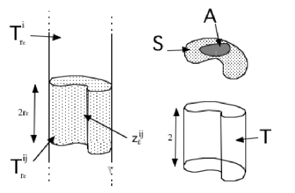
Figure 2. The set $T_{r_{\varepsilon}}^{ij}$.

and setting for every ${\boldsymbol{\varphi}}\in L^{p}(\Omega;\mathbb{R}^{3})$,

$${{\textswab{\boldsymbol{v}}}}_{\varepsilon}({\boldsymbol{\varphi}})(x):=\hskip-8.5359pt\sum_{(i,j)\in{I}_{\varepsilon}\times L_{\varepsilon}}\hskip-5.69046pt\left({\int\!\!\!\!\!\!-}_{T_{r_{\varepsilon}}^{ij}}\widehat{\boldsymbol{\varphi}}(s)d{\mathcal{L}}^{3}(s)\right)\mathds{1}_{Y_{\varepsilon}^{i}\times\Delta_{r_{\varepsilon}}^{j}}(x);\quad\theta_{\varepsilon}({\boldsymbol{\varphi}}):={{\mathfrak{w}}}_{\varepsilon 3}({\boldsymbol{\varphi}}),$$ (5.6)

$${{\textswab{\boldsymbol{w}}}}_{\varepsilon}({\boldsymbol{\varphi}})(x)\!:=\hskip-14.22636pt\sum_{(i,j)\in{I}_{\varepsilon}\times L_{\varepsilon}}\hskip-5.69046pt\left(\frac{{\rm diam}S}{2}\boldsymbol{M}{\int\!\!\!\!\!\!-}_{T_{r_{\varepsilon}}^{ij}}\!\!\!\left(\frac{\boldsymbol{z}_{\varepsilon}(s)}{r_{\varepsilon}}\wedge\widehat{\boldsymbol{\varphi}}(s)\right)\hskip-2.84544ptd{\mathcal{L}}^{3}(s)\hskip-2.84544pt\right)\hskip-2.84544pt\mathds{1}_{Y_{\varepsilon}^{i}\times\Delta_{r_{\varepsilon}}^{j}}(x),$$

$$\boldsymbol{M}:=\sum_{i,j,k=1}^{3}\frac{1}{2}\varepsilon_{ijk}^{2}\left({\int\!\!\!\!\!\!-}_{T}z_{i}^{2}+z_{j}^{2}d{\mathcal{L}}^{3}(z)\right)^{-1}\boldsymbol{e}_{k}\otimes\boldsymbol{e}_{k},$$

$${{\textswab{\boldsymbol{r}}}}_{\varepsilon}({\boldsymbol{\varphi}}):={{\textswab{\boldsymbol{v}}}}_{\varepsilon}({\boldsymbol{\varphi}})+\frac{2}{{\rm diam}S}{{\textswab{\boldsymbol{w}}}}_{\varepsilon}({\boldsymbol{\varphi}})\wedge\frac{\boldsymbol{z}_{\varepsilon}(x)}{r_{\varepsilon}},$$

where $\widehat{\boldsymbol{\varphi}}$ is an extension of ${\boldsymbol{\varphi}}$ (see (5.47)) bringing meaning to ${\int\!\!\!\!-}_{T_{r_{\varepsilon}}^{ij^{m}}}\widehat{\boldsymbol{\varphi}}$ where

$$j^{m}_{\varepsilon}:=\max L_{\varepsilon}.$$ (5.7)

We will prove that the piecewise rigid motion ${{\textswab{\boldsymbol{r}}}}_{\varepsilon}(\boldsymbol{u}_{\varepsilon})$ approximates to the velocity in each set $T_{r_{\varepsilon}}^{ij}$ and asymptotically behaves as $\overline{{\textswab{\boldsymbol{r}}}}_{\varepsilon}^{S}(\boldsymbol{u}_{\varepsilon})$. To derive formula (1.13), we will employ the auxiliary field $\overline{{\textswab{\boldsymbol{u}}}}_{\varepsilon}(\boldsymbol{u}_{\varepsilon})$ defined by

$$\overline{{\textswab{\boldsymbol{u}}}}_{\varepsilon}({\boldsymbol{\varphi}})(x)\!:=\!\sum_{i\in I_{\varepsilon}}\left({\int\!\!\!\!\!\!-}_{D_{R_{\varepsilon}}^{i}\setminus D_{R_{\varepsilon}\!/2}^{i}}\!\!{\boldsymbol{\varphi}}(s,x_{3})d{\mathcal{H}}^{2}(s)\right)\mathds{1}_{Y_{\varepsilon}^{i}}(x^{\prime})$$ (5.8)

in terms of a sequence $(R_{\varepsilon})$ satisfying (3.17). The assumption (3.17) ensures that $(\overline{{\textswab{\boldsymbol{u}}}}_{\varepsilon}(\boldsymbol{u}_{\varepsilon}))$ approximates to $\boldsymbol{u}_{\varepsilon}$ in $\Omega$. The selection of integrals over $D_{R_{\varepsilon}}^{i}\setminus D_{R_{\varepsilon}\!/2}^{i}$ in (5.8) will yield a crucial estimate at a technical step.

5.2. Two-scale convergence with respect to $(m_{\varepsilon})$

To particularize the effective behavior of $\boldsymbol{u}_{\varepsilon}$ in the fibers, we introduce variant of the two-scale convergence [1, 29, 45] defined in terms of the measures

$$m_{\varepsilon}:=\frac{\varepsilon^{2}}{r_{\varepsilon}^{2}|S|}\mathds{1}_{S_{r_{\varepsilon}}\times(0,L)}{\mathcal{L}}^{3}_{\lfloor\Omega}$$ (5.9)

which are supported on the fibers and weakly^⋆ converging in ${\mathcal{M}}(\overline{\Omega})$ to ${\mathcal{L}}^{3}_{\lfloor\Omega}$. We say that a sequence $({\boldsymbol{\varphi}}_{\varepsilon})$ in $L^{p}(\Omega;\mathbb{R}^{k})$ two-scale converges to ${\boldsymbol{\varphi}}_{0}\in L^{p}(\Omega\times S;\mathbb{R}^{k})$ with respect to $(m_{\varepsilon})$ if (see (3.11))

$$\lim_{\varepsilon\to 0}\int{\boldsymbol{\varphi}}_{\varepsilon}(x)\cdot{\boldsymbol{\eta}}\left(x,\frac{y_{\varepsilon}(x^{\prime})}{r_{\varepsilon}}\right) dm_{\varepsilon}(x)=\frac{1}{|S|}\int_{\Omega\times S}{\boldsymbol{\varphi}}_{0}(x,y)\cdot{\boldsymbol{\eta}}(x,y)dxdy,$$ (5.10)

$$\ \forall\,{\boldsymbol{\eta}}\in C(\overline{\Omega\times S};\mathbb{R}^{k})\quad\hbox{(notation: ${\boldsymbol{\varphi}}_{\varepsilon}{\,\buildrel m_{\varepsilon}\over{\rightharpoonup\!\!\!\!\!\!\!\!\rightharpoonup}\,}{\boldsymbol{\varphi}}_{0}$)}.$$

The main properties of this convergence are stated in the following Lemma.

Lemma 1.

For every ${\boldsymbol{\eta}}\in C(\overline{\Omega};L^{\infty}(S;\mathbb{R}^{k}))$,

$$\lim_{\varepsilon\to 0}\int{\boldsymbol{\eta}}\left(x,\frac{y_{\varepsilon}(x^{\prime})}{r_{\varepsilon}}\right)dm_{\varepsilon}(x)=\frac{1}{|S|}\int_{\Omega\times S}{\boldsymbol{\eta}}(x,y)dxdy.$$ (5.11)

Any sequence $({\boldsymbol{\varphi}}_{\varepsilon})$ in $L^{p}(\Omega;\mathbb{R}^{k})$ such that

$$\sup_{\varepsilon>0}\int|{\boldsymbol{\varphi}}_{\varepsilon}|^{p}dm_{\varepsilon}\leq C,$$ (5.12)

two-scale converges w.r.t. $(m_{\varepsilon})$, up to a subsequence, to some ${\boldsymbol{\varphi}}_{0}$. Setting ${\boldsymbol{\varphi}}(x):=\frac{1}{|S|}\int_{S}{\boldsymbol{\varphi}}_{0}(x,y)dy$, the following implications holds:

$${\boldsymbol{\varphi}}_{\varepsilon}{\,\buildrel m_{\varepsilon}\over{\rightharpoonup\!\!\!\!\!\!\!\!\rightharpoonup}\,}{\boldsymbol{\varphi}}_{0}\quad\Longrightarrow\quad{\boldsymbol{\varphi}}_{\varepsilon}{\boldsymbol{\eta}}\left(x,\frac{y_{\varepsilon}(x^{\prime})}{r_{\varepsilon}}\right){\,\buildrel m_{\varepsilon}\over{\rightharpoonup\!\!\!\!\!\!\!\!\rightharpoonup}\,}\ {\boldsymbol{\varphi}}_{0}{\boldsymbol{\eta}}\qquad\forall{\boldsymbol{\eta}}\in C(\overline{\Omega\times S};\mathbb{R}^{k}),$$ (5.13)

$${\boldsymbol{\varphi}}_{\varepsilon}{\,\buildrel m_{\varepsilon}\over{\rightharpoonup\!\!\!\!\!\!\!\!\rightharpoonup}\,}{\boldsymbol{\varphi}}_{0}\quad\Longrightarrow\quad{\boldsymbol{\varphi}}_{\varepsilon}m_{\varepsilon}\buildrel\star\over{\rightharpoonup}{\boldsymbol{\varphi}}\ \ \hbox{weakly${}^{\star}$ in }\ {\mathcal{M}}(\overline{\Omega};\!\mathbb{R}^{k}).$$ (5.14)

If ${\boldsymbol{\varphi}}_{\varepsilon}{\,\buildrel m_{\varepsilon}\over{\rightharpoonup\!\!\!\!\!\!\!\!\rightharpoonup}\,}{\boldsymbol{\varphi}}_{0}$, for any convex function $j:\mathbb{R}^{k}\to\mathbb{R}$, we have

$$\liminf_{\varepsilon\to 0}\int j({\boldsymbol{\varphi}}_{\varepsilon})dm_{\varepsilon}\geq\frac{1}{|S|}\int_{\Omega\times S}\hskip-5.69046ptj({\boldsymbol{\varphi}}_{0})dxdy\geq\int_{\Omega}j({\boldsymbol{\varphi}})dx.$$ (5.15)

Proof. The proof of (5.11) is similar to that of [1, Lemma 1.3]. Setting $\int{\boldsymbol{\eta}}\cdot d{\boldsymbol{\nu}}_{\varepsilon}:=\int{\boldsymbol{\varphi}}_{\varepsilon}(x)\cdot{\boldsymbol{\eta}}\left(x,\frac{y_{\varepsilon}(x^{\prime})}{r_{\varepsilon}}\right)dm_{\varepsilon}(x)$ $\forall{\boldsymbol{\eta}}\in C(\overline{\Omega\times S};\mathbb{R}^{k})$, the two-scale convergence w.r.t. $(m_{\varepsilon})$ of $({\boldsymbol{\varphi}}_{\varepsilon})$ to ${\boldsymbol{\varphi}}_{0}$ is equivalent to the weak^⋆ convergence in ${\mathcal{M}}(\overline{\Omega\times S})$ of $(\nu_{\varepsilon})$ to $\frac{1}{|S|}{\boldsymbol{\varphi}}_{0}(x,y){\mathcal{L}}^{5}_{\lfloor\Omega\times S}$. By (5.12) and Hölder’s inequality, we have

$$\left|\int{\boldsymbol{\eta}}\cdot d{\boldsymbol{\nu}}_{\varepsilon}\right|\leq C\left(\int\left|{\boldsymbol{\eta}}\left(x,\frac{y_{\varepsilon}(x^{\prime})}{r_{\varepsilon}}\right)\right|^{p^{\prime}}dm_{\varepsilon}(x)\right)^{\frac{1}{p^{\prime}}}\!\!\leq C|{\boldsymbol{\eta}}|_{L^{\infty}(\Omega\times S;\mathbb{R}^{k})},$$ (5.16)

thus $({\boldsymbol{\nu}}_{\varepsilon})$, bounded in ${\mathcal{M}}(\overline{\Omega\times S};\mathbb{R}^{k})$, weakly^⋆ converges up to a subsequence to some ${\boldsymbol{\nu}}$. Passing to the limit in (5.16), taking (5.11) into account, we obtain $\left|\int{\boldsymbol{\eta}}\cdot d{\boldsymbol{\nu}}\right|\leq C\left(\int_{\Omega\times S}\left|{\boldsymbol{\eta}}\left(x,y\right)\right|^{p^{\prime}}dxdy\right)^{\frac{1}{p^{\prime}}}$, hence, by the Riesz representation theorem ${\boldsymbol{\nu}}=\frac{1}{|S|}{\boldsymbol{\varphi}}_{0}(x,y){\mathcal{L}}^{5}_{\lfloor\Omega\times S}$ for some ${\boldsymbol{\varphi}}_{0}\in L^{p}(\Omega\times S;\mathbb{R}^{k})$. The assertion (5.13) is straightforward. By choosing in (5.10) test fields independent of $y$, we obtain (5.14). Denoting by $j^{\star}$ the Fenchel transform of $j$, we deduce from Fenchel’s inequality, (5.10) and (5.11), that

$$\liminf_{\varepsilon\to 0}\int\!j({\boldsymbol{\varphi}}_{\varepsilon})dm_{\varepsilon}(x) \geq\lim_{\varepsilon\to 0}\int{\boldsymbol{\varphi}}_{\varepsilon}\cdot{\boldsymbol{\eta}}\left(x,\frac{y_{\varepsilon}(x^{\prime})}{r_{\varepsilon}}\right)\!-j^{\star}\left({\boldsymbol{\eta}}\left(x,\frac{y_{\varepsilon}(x^{\prime})}{r_{\varepsilon}}\right)\hskip-2.84544pt\right)\hskip-2.84544ptdm_{\varepsilon}(x)$$

$$=\frac{1}{|S|}\int_{\Omega\times S}{\boldsymbol{\varphi}}_{0}\cdot{\boldsymbol{\eta}}-j^{\star}({\boldsymbol{\eta}})dxdy\qquad\forall{\boldsymbol{\eta}}\in C(\overline{\Omega\times S};\mathbb{R}^{k}).$$

Noticing that by the convexity of $j$ we have $j^{\star\star}=j$, we infer

$$\liminf_{\varepsilon\to 0}\int\!j({\boldsymbol{\varphi}}_{\varepsilon})dm_{\varepsilon}(x) \geq\sup_{{\boldsymbol{\eta}}\in C(\overline{\Omega\times S};\mathbb{R}^{k})}\frac{1}{|S|}\int_{\Omega\times S}{\boldsymbol{\varphi}}_{0}\cdot{\boldsymbol{\eta}}-j^{\star}({\boldsymbol{\eta}})dxdy$$ (5.17)

$$=\frac{1}{|S|}\int_{\Omega\times S}\ \sup_{{\boldsymbol{\eta}}\in\mathbb{R}^{k}}\{{\boldsymbol{\varphi}}_{0}\cdot{\boldsymbol{\eta}}-j^{\star}({\boldsymbol{\eta}})\}dxdy$$

$$=\frac{1}{|S|}\int_{\Omega\times S}j^{\star\star}({\boldsymbol{\varphi}}_{0})dxdy=\frac{1}{|S|}\int_{\Omega\times S}j({\boldsymbol{\varphi}}_{0})dxdy,$$

the second line being justified in Remark 7. The second inequality in (5.15) results from (5.14) and Jensen’s inequality. ∎

Remark 5.

Combining Lemma 1 with [11, Lemma 4.2], one can derive a non-periodic version of Lemma 1 adapted for the proof of Theorem 3.

5.3. Properties of the auxiliary sequences

In this section, we compare diverse types of convergence for the auxiliary sequences $({{\textswab{\boldsymbol{p}}}}_{\varepsilon}(\boldsymbol{u}_{\varepsilon}))$ introduced in Section 5.1. It turns out that, except for ${{\textswab{\boldsymbol{p}}}}_{\varepsilon}\in\{{{\textswab{\boldsymbol{r}}}}_{\varepsilon},\overline{{\textswab{\boldsymbol{r}}}}_{\varepsilon}^{S}\}$, the weak limit of $({{\textswab{\boldsymbol{p}}}}_{\varepsilon}(\boldsymbol{u}_{\varepsilon}))$ in $L^{p}$, its two-scale limits w.r.t. to $(m_{\varepsilon})$ and the weak* limits of $({{\textswab{\boldsymbol{p}}}}_{\varepsilon}(\boldsymbol{u}_{\varepsilon})m_{\varepsilon})$ in ${\mathcal{M}}(\overline{\Omega})$ are the same, and that $(\overline{{\textswab{\boldsymbol{v}}}}_{\varepsilon}^{S}(\boldsymbol{u}_{\varepsilon}))$ and $({{\textswab{\boldsymbol{v}}}}_{\varepsilon}(\boldsymbol{u}_{\varepsilon}))$ have the same weak limits in $L^{p}$. We will prove in Proposition 3 that the same holds for $(\overline{\theta}_{\varepsilon}^{S}(\boldsymbol{u}_{\varepsilon})\boldsymbol{e}_{3})$ and $({{\textswab{\boldsymbol{w}}}}_{\varepsilon}(\boldsymbol{u}_{\varepsilon}))$. This, combined with (5.23), shows that $(\overline{{\textswab{\boldsymbol{r}}}}_{\varepsilon}^{S}(\boldsymbol{u}_{\varepsilon}))$ and $({{\textswab{\boldsymbol{r}}}}_{\varepsilon}(\boldsymbol{u}_{\varepsilon}))$ have the same two-scale limits w.r.t. $(m_{\varepsilon})$.

Proposition 1.

Let ${{\textswab{\boldsymbol{p}}}}_{\varepsilon}$ be a linear combination of ${{\textswab{\boldsymbol{w}}}}_{\varepsilon}$, ${{\textswab{\boldsymbol{v}}}}_{\varepsilon}$, $\theta_{\varepsilon}\boldsymbol{e}_{3}$, ${\overline{{\textswab{\boldsymbol{v}}}}}^{A}_{\varepsilon}$, ${\overline{\theta}}^{A}_{\varepsilon}\boldsymbol{e}_{3}$, $\overline{{\textswab{\boldsymbol{u}}}}_{\varepsilon}$ defined by (5.4), (5.6), (5.8), and $({\boldsymbol{\varphi}}_{\varepsilon})$ a sequence in $L^{p}(\Omega;\mathbb{R}^{3})$ satisfying (5.12).
(i) For all ${\boldsymbol{\varphi}}\in W^{1,p}(\Omega;\mathbb{R}^{3})$, $\varepsilon>0$, $k\in\{1,2,3\}$, we have

$$\int|{{\textswab{\boldsymbol{p}}}}_{\varepsilon}({\boldsymbol{\varphi}})|^{p}dm_{\varepsilon}=\int_{\Omega}|{{\textswab{\boldsymbol{p}}}}_{\varepsilon}({\boldsymbol{\varphi}})|^{p}dx,$$ (5.18)

$$\int|{{\textswab{\boldsymbol{p}}}}_{\varepsilon}({\boldsymbol{\varphi}})|^{p}dm_{\varepsilon}\leq C\int_{\Omega}|{\boldsymbol{\varphi}}|^{p}dm_{\varepsilon},\quad\int|\overline{{\mathfrak{v}}}^{A}_{\varepsilon k}({\boldsymbol{\varphi}})|^{p}dm_{\varepsilon}\leq\frac{|S|}{|A|}\int_{\Omega}|\varphi_{k}|^{p}dm_{\varepsilon}.$$ (5.19)

(ii) For every $\boldsymbol{p}\in L^{p}(\Omega;\mathbb{R}^{3})$, the following equivalences hold

$$\hskip-5.69046pt{\boldsymbol{\varphi}}_{\varepsilon}m_{\varepsilon}\ \buildrel\star\over{\rightharpoonup}\ \boldsymbol{p}\hbox{ weakly${}^{\star}$ in }{\mathcal{M}}(\overline{\Omega};\mathbb{R}^{3}) \Longleftrightarrow\ \ \overline{{\textswab{\boldsymbol{v}}}}_{\varepsilon}^{S}({\boldsymbol{\varphi}}_{\varepsilon})\!\rightharpoonup\!\boldsymbol{p}\hbox{ weakly in }L^{p}(\Omega;\mathbb{R}^{3})$$ (5.20)

$$\Longleftrightarrow\ \ {{\textswab{\boldsymbol{v}}}}_{\varepsilon}({\boldsymbol{\varphi}}_{\varepsilon})\!\rightharpoonup\!\boldsymbol{p}\hbox{ weakly in }L^{p}(\Omega;\mathbb{R}^{3}).$$

(iii) If $({{\textswab{\boldsymbol{p}}}}_{\varepsilon}({\boldsymbol{\varphi}}_{\varepsilon}))$ two-scale converges to $\boldsymbol{p}_{0}$ w.r.t. $(m_{\varepsilon})$, then $\boldsymbol{p}_{0}(x,y)=\boldsymbol{p}(x)$ a. e. in $\Omega\times S$ for some $\boldsymbol{p}\in L^{p}(\Omega;\mathbb{R}^{3})$. Furthermore, for every $\boldsymbol{p}\in L^{p}(\Omega;\mathbb{R}^{3})$,

$${{\textswab{\boldsymbol{p}}}}_{\varepsilon}({\boldsymbol{\varphi}}_{\varepsilon}){\,\buildrel m_{\varepsilon}\over{\rightharpoonup\!\!\!\!\!\!\!\!\rightharpoonup}\,}\boldsymbol{p}\quad\Longleftrightarrow\quad{{\textswab{\boldsymbol{p}}}}_{\varepsilon}({\boldsymbol{\varphi}}_{\varepsilon})m_{\varepsilon}\ \buildrel\star\over{\rightharpoonup}\ \boldsymbol{p}\hbox{ weakly${}^{\star}$ in }{\mathcal{M}}(\overline{\Omega};\mathbb{R}^{3})$$ (5.21)

$$\Longleftrightarrow\ {{\textswab{\boldsymbol{p}}}}_{\varepsilon}({\boldsymbol{\varphi}}_{\varepsilon})\!\rightharpoonup\!\boldsymbol{p}\hbox{ weakly in }L^{p}(\!\Omega;\mathbb{R}^{3})\Longrightarrow\left({{\textswab{\boldsymbol{p}}}}_{\varepsilon}({\boldsymbol{\varphi}}_{\varepsilon})\wedge\frac{\boldsymbol{y}_{\varepsilon}(x^{\prime})}{r_{\varepsilon}}\right){\,\buildrel m_{\varepsilon}\over{\rightharpoonup\!\!\!\!\!\!\!\!\rightharpoonup}\,}\ \boldsymbol{p}\wedge\boldsymbol{y}.$$

(iv) If $\,{{\textswab{\boldsymbol{p}}}}_{\varepsilon}$ is a linear combination of ${{\textswab{\boldsymbol{w}}}}_{\varepsilon}$, ${{\textswab{\boldsymbol{v}}}}_{\varepsilon}$, $\theta_{\varepsilon}\boldsymbol{e}_{3}$, then

$${{\textswab{\boldsymbol{p}}}}_{\varepsilon}({\boldsymbol{\varphi}}_{\varepsilon})\!\rightharpoonup\!\boldsymbol{p}\hbox{ weakly in }L^{p}(\!\Omega;\mathbb{R}^{3}) \Longrightarrow\left({{\textswab{\boldsymbol{p}}}}_{\varepsilon}({\boldsymbol{\varphi}}_{\varepsilon})\wedge\frac{\boldsymbol{z}_{\varepsilon}(x)}{r_{\varepsilon}}\right){\,\buildrel m_{\varepsilon}\over{\rightharpoonup\!\!\!\!\!\!\!\!\rightharpoonup}\,}\boldsymbol{p}\wedge\boldsymbol{y},$$ (5.22)

where $\boldsymbol{z}_{\varepsilon}(x)$ is defined by (5.5). In particular, the following holds:

$$\left.\begin{aligned} &{{\textswab{\boldsymbol{v}}}}_{\varepsilon}({\boldsymbol{\varphi}}_{\varepsilon})\!\rightharpoonup\!\boldsymbol{v}&&\hbox{weakly in }L^{p}(\Omega;\mathbb{R}^{3})\\ &{{\textswab{\boldsymbol{w}}}}_{\varepsilon}({\boldsymbol{\varphi}}_{\varepsilon})\!\rightharpoonup\!\boldsymbol{w}&&\hbox{weakly in }L^{p}(\Omega;\mathbb{R}^{3})\end{aligned}\right\}\Longrightarrow{{\textswab{\boldsymbol{r}}}}_{\varepsilon}({\boldsymbol{\varphi}}_{\varepsilon}){\,\buildrel m_{\varepsilon}\over{\rightharpoonup\!\!\!\!\!\!\!\!\rightharpoonup}\,}\boldsymbol{v}+\frac{2}{{\rm diam}S}\boldsymbol{w}\wedge\boldsymbol{y}.$$ (5.23)

Proof. (i) Since ${{\textswab{\boldsymbol{p}}}}_{\varepsilon}({\boldsymbol{\varphi}})$ is constant in each set $Y_{\varepsilon}^{i}\times\{x_{3}\}$, by (3.3) and (5.9),

$$\int|{{\textswab{\boldsymbol{p}}}}_{\varepsilon}({\boldsymbol{\varphi}})|^{p}dm_{\varepsilon} =\frac{\varepsilon^{2}}{r_{\varepsilon}^{2}|S|}\int_{T_{r_{\varepsilon}}}|{{\textswab{\boldsymbol{p}}}}_{\varepsilon}({\boldsymbol{\varphi}})|^{p}dx=\frac{\varepsilon^{2}}{r_{\varepsilon}^{2}|S|}\sum_{i\in I_{\varepsilon}}\int_{0}^{L}dx_{3}\int_{S_{r_{\varepsilon}}^{i}}|{{\textswab{\boldsymbol{p}}}}_{\varepsilon}({\boldsymbol{\varphi}})|^{p}dx^{\prime}$$

$$=\frac{\varepsilon^{2}}{r_{\varepsilon}^{2}|S|}\sum_{i\in I_{\varepsilon}}\int_{0}^{L}dx_{3}\frac{|S_{r_{\varepsilon}}^{i}|}{|Y_{\varepsilon}^{i}|}\int_{Y_{\varepsilon}^{i}}|{{\textswab{\boldsymbol{p}}}}_{\varepsilon}({\boldsymbol{\varphi}})|^{p}dx^{\prime}=\int_{\Omega}|{{\textswab{\boldsymbol{p}}}}_{\varepsilon}({\boldsymbol{\varphi}})|^{p}dx.$$

We deduce from (5.3), (5.4), (5.9) and Jensen’s inequality, that for $k\in\{1,2,3\}$,

$$\int|\overline{{\mathfrak{v}}}^{A}_{\varepsilon k}({\boldsymbol{\varphi}})|^{p}dm_{\varepsilon} =\frac{\varepsilon^{2}}{r_{\varepsilon}^{2}|S|}\sum_{i\in I_{\varepsilon}}\int_{0}^{L}dx_{3}\int_{S_{r_{\varepsilon}}^{i}}\left|{\int\!\!\!\!\!\!-}_{A_{r_{\varepsilon}}^{i}}\varphi_{k}(s^{\prime},x_{3})d{\mathcal{H}}^{2}(s^{\prime})\right|^{p}dx^{\prime}$$

$$\hskip-56.9055pt\leq\frac{\varepsilon^{2}}{r_{\varepsilon}^{2}|S|}\sum_{i\in I_{\varepsilon}}\int_{0}^{L}dx_{3}\frac{|S_{r_{\varepsilon}}^{i}|}{|A_{r_{\varepsilon}}^{i}|}\int_{S_{r_{\varepsilon}}^{i}}|\varphi_{k}|^{p}(s^{\prime},x_{3})d{\mathcal{H}}^{2}(s^{\prime})=\frac{|S|}{|A|}\int_{\Omega}|\varphi_{k}|^{p}dm_{\varepsilon}.$$

The inequality $\int|{{\textswab{\boldsymbol{p}}}}_{\varepsilon}({\boldsymbol{\varphi}})|^{p}dm_{\varepsilon}\leq C\int_{\Omega}|{\boldsymbol{\varphi}}|^{p}dm_{\varepsilon}$ is obtained in a similar way. ∎

(ii) We fix ${\boldsymbol{\psi}}\in{\mathcal{D}}(\Omega;\mathbb{R}^{3})$ and set (see (5.5), (5.7))

$$\ {\boldsymbol{\psi}}^{(\varepsilon)}(x):=\sum_{(i,j)\in I_{\varepsilon}\times(L_{\varepsilon}\setminus\{j^{m}_{\varepsilon}\})}\left({\int\!\!\!\!\!\!-}_{Y_{\varepsilon}^{i}\times\Delta_{\varepsilon}^{j}}{\boldsymbol{\psi}}d{\mathcal{L}}^{3}\right)\mathds{1}_{Y_{\varepsilon}^{i}\times\Delta_{\varepsilon}^{j}}(x).$$ (5.24)

As ${\boldsymbol{\psi}}$ is compactly supported in $\Omega$, the following estimate holds:

$$|{\boldsymbol{\psi}}^{(\varepsilon)}-{\boldsymbol{\psi}}|_{L^{\infty}(\Omega;\mathbb{R}^{3})}<C\varepsilon.$$ (5.25)

Taking (5.4), (5.6), (5.8), (5.9), and the constant nature of ${\boldsymbol{\psi}}^{(\varepsilon)}$ in each set $Y_{\varepsilon}^{i}\times\Delta_{\varepsilon}^{j}$ into account, elementary computations yield

$$\begin{aligned} &\int{\boldsymbol{\psi}}^{(\varepsilon)}\hskip-2.84544pt\cdot\overline{{\textswab{\boldsymbol{v}}}}^{S}_{\varepsilon}({\boldsymbol{\varphi}}_{\varepsilon})dm_{\varepsilon}=\int{\boldsymbol{\psi}}^{(\varepsilon)}\cdot{\boldsymbol{\varphi}}_{\varepsilon}dm_{\varepsilon},\\ &\int{\boldsymbol{\psi}}^{(\varepsilon)}\cdot{{\textswab{\boldsymbol{v}}}}_{\varepsilon}({\boldsymbol{\varphi}}_{\varepsilon})dm_{\varepsilon}=\int{\boldsymbol{\psi}}^{(\varepsilon)}\cdot{\boldsymbol{\varphi}}_{\varepsilon}dm_{\varepsilon},\end{aligned}$$ (5.26)

$$\begin{aligned} \int{\boldsymbol{\psi}}^{(\varepsilon)}\cdot\ &{{\textswab{\boldsymbol{p}}}}_{\varepsilon}({\boldsymbol{\varphi}}_{\varepsilon})dm_{\varepsilon}=\int_{\Omega}{\boldsymbol{\psi}}^{(\varepsilon)}\cdot{{\textswab{\boldsymbol{p}}}}_{\varepsilon}({\boldsymbol{\varphi}}_{\varepsilon})dx.\end{aligned}$$ (5.27)

By (5.12), (5.19) and Lemma 1, the sequences $({\boldsymbol{\varphi}}_{\varepsilon}m_{\varepsilon})$, $(\overline{{\textswab{\boldsymbol{v}}}}_{\varepsilon}^{S}({\boldsymbol{\varphi}}_{\varepsilon})m_{\varepsilon})$, and $({{\textswab{\boldsymbol{v}}}}_{\varepsilon}({\boldsymbol{\varphi}}_{\varepsilon})m_{\varepsilon})$ weakly^⋆ converge in ${\mathcal{M}}(\overline{\Omega};\mathbb{R}^{3})$, up to a subsequence, to $\boldsymbol{p}_{1}$, $\boldsymbol{p}_{2}$, and $\boldsymbol{p}_{3}$, respectively, for some $\boldsymbol{p}_{i}\in L^{p}(\Omega;\mathbb{R}^{3})$. By passing to the limit as $\varepsilon\to 0$ in (5.26), taking (5.25) into account, we infer $\int_{\Omega}{\boldsymbol{\psi}}\cdot\boldsymbol{p}_{1}dx=\int_{\Omega}{\boldsymbol{\psi}}\cdot\boldsymbol{p}_{2}dx=\int_{\Omega}{\boldsymbol{\psi}}\cdot\boldsymbol{p}_{3}dx$ and deduce from the arbitrariness of ${\boldsymbol{\psi}}$ that $\boldsymbol{p}_{1}=\boldsymbol{p}_{2}=\boldsymbol{p}_{3}$. ∎

(iii) Assume that ${{\textswab{\boldsymbol{p}}}}_{\varepsilon}({\boldsymbol{\varphi}}_{\varepsilon})\hskip-1.42271pt{\,\buildrel m_{\varepsilon}\over{\rightharpoonup\!\!\!\!\!\!\!\!\rightharpoonup}\,}\boldsymbol{p}_{0}$ for some $\boldsymbol{p}_{0}\in L^{p}(\Omega\times Y;\mathbb{R}^{3})$. Since ${{\textswab{\boldsymbol{p}}}}_{\varepsilon}({\boldsymbol{\varphi}}_{\varepsilon})$ is constant in each set $Y_{\varepsilon}^{i}\times\{x_{3}\}$, for any $\boldsymbol{\Psi}\in{\mathcal{D}}(\Omega\times S;\mathbb{R}^{3}\times\mathbb{R}^{3})$ we have $\displaystyle\int{{\textswab{\boldsymbol{p}}}}_{\varepsilon}({\boldsymbol{\varphi}}_{\varepsilon})\cdot{\rm\bf div}_{y}\boldsymbol{\Psi}\Big{(}x,\frac{y_{\varepsilon}(x^{\prime})}{r_{\varepsilon}}\Big{)}dm_{\varepsilon}=0$. Passing to the limit as $\varepsilon\to 0$, we get $\displaystyle\frac{1}{|S|}\int_{\Omega\times S}\hskip-11.38092pt\boldsymbol{p}_{0}\cdot{\rm\bf div}_{y}\boldsymbol{\Psi}dxdy=0$ and deduce from the arbitrary choice of $\boldsymbol{\Psi}$ that $\boldsymbol{p}_{0}(x,y)=\boldsymbol{p}(x)$ a.e. in $\Omega\times S$, where $\boldsymbol{p}(x):={\int\!\!\!\!\!\!-}_{S}\boldsymbol{p}_{0}(x,y)dy\in L^{p}(\Omega;\mathbb{R}^{3})$. It follows from (5.14) that ${{\textswab{\boldsymbol{p}}}}_{\varepsilon}({\boldsymbol{\varphi}}_{\varepsilon})m_{\varepsilon}\!\buildrel\star\over{\rightharpoonup}\!\boldsymbol{p}{\mathcal{L}}^{3}$ weakly^⋆ in ${\mathcal{M}}(\overline{\Omega};\mathbb{R}^{3})$. On the other hand, by (5.12), (5.18), and (5.19), $({{\textswab{\boldsymbol{p}}}}_{\varepsilon}({\boldsymbol{\varphi}}_{\varepsilon}))$ is bounded in $L^{p}(\Omega;\mathbb{R}^{3})$ and weakly converges, up to a subsequence, to some $\tilde{\boldsymbol{p}}$. By passing to the limit as $\varepsilon\to 0$ in (5.27), taking (5.25) into account, we obtain $\int_{\Omega}{\boldsymbol{\psi}}\cdot\boldsymbol{p}dx=\int_{\Omega}{\boldsymbol{\psi}}\cdot\tilde{\boldsymbol{p}}dx$ and deduce $\boldsymbol{p}=\tilde{\boldsymbol{p}}$. Conversely, if ${{\textswab{\boldsymbol{p}}}}_{\varepsilon}({\boldsymbol{\varphi}}_{\varepsilon})\rightharpoonup\boldsymbol{p}$ weakly in $L^{p}(\Omega;\mathbb{R}^{3})$, then by (5.12), (5.19) and Lemma 1, $({{\textswab{\boldsymbol{p}}}}_{\varepsilon}({\boldsymbol{\varphi}}_{\varepsilon}))$ two-scale converges w.r.t. $(m_{\varepsilon})$, up to a subsequence, to some element of $L^{p}(\Omega;\mathbb{R}^{3})$ which, by virtue of the last established implications, necessarily equals $\boldsymbol{p}$. The equivalences stated in (5.21) are proved and the implication is obtained by choosing $\boldsymbol{y}\wedge{\boldsymbol{\eta}}\left(x,y\right)$ as a test function for the two-scale convergence of $({{\textswab{\boldsymbol{p}}}}_{\varepsilon}({\boldsymbol{\varphi}}_{\varepsilon}))$ to $\boldsymbol{p}$ w.r.t. $(m_{\varepsilon})$.

(iv) Assume that ${{\textswab{\boldsymbol{p}}}}_{\varepsilon}$ is a linear combination of ${{\textswab{\boldsymbol{w}}}}_{\varepsilon}$, ${{\textswab{\boldsymbol{v}}}}_{\varepsilon}$, $\theta_{\varepsilon}\boldsymbol{e}_{3}$ and ${{\textswab{\boldsymbol{p}}}}_{\varepsilon}({\boldsymbol{\varphi}}_{\varepsilon})\rightharpoonup\boldsymbol{p}$ weakly in $L^{p}(\Omega;\mathbb{R}^{3})$. By (5.12) and (5.19), $\int\left|{{\textswab{\boldsymbol{p}}}}_{\varepsilon}({\boldsymbol{\varphi}}_{\varepsilon})\wedge\frac{\boldsymbol{z}_{\varepsilon}}{r_{\varepsilon}}\right|^{p}dm_{\varepsilon}\leq C$, hence, by Lemma 1, $\left({{\textswab{\boldsymbol{p}}}}_{\varepsilon}({\boldsymbol{\varphi}}_{\varepsilon})\wedge\frac{\boldsymbol{z}_{\varepsilon}}{r_{\varepsilon}}\right){\,\buildrel m_{\varepsilon}\over{\rightharpoonup\!\!\!\!\!\!\!\!\rightharpoonup}\,}\boldsymbol{q}_{0}$, up to a subsequence, for some $\boldsymbol{q}_{0}$. We fix ${\boldsymbol{\eta}}\in{\mathcal{D}}(\Omega\times S;\mathbb{R}^{3})$ and set

$${\boldsymbol{\eta}}^{[\varepsilon]}(x,y):=\sum_{(i,j)\in I_{\varepsilon}\times(L_{\varepsilon}\setminus\{j^{m}_{\varepsilon}\})}\left({\int\!\!\!\!\!\!-}_{Y_{\varepsilon}^{i}\times\Delta_{\varepsilon}^{j}}{\boldsymbol{\eta}}(s,y)d{\mathcal{H}}^{3}(s)\right)\mathds{1}_{Y_{\varepsilon}^{i}\times\Delta_{\varepsilon}^{j}}(x).$$ (5.28)

The fields ${{\textswab{\boldsymbol{p}}}}_{\varepsilon}({\boldsymbol{\varphi}}_{\varepsilon})$ and ${\boldsymbol{\eta}}^{[\varepsilon]}\left(x,\frac{y_{\varepsilon}(x^{\prime})}{r_{\varepsilon}}\right)$ are independent of $x_{3}$ in each $Y_{\varepsilon}^{i}\times\Delta_{\varepsilon}^{j}$ and, by (3.11) and (5.5), $\int_{\Delta_{\varepsilon}^{j}}\boldsymbol{z}_{\varepsilon}(x^{\prime},x_{3})dx_{3}=\int_{\Delta_{\varepsilon}^{j}}\boldsymbol{y}_{\varepsilon}(x^{\prime})dx_{3}$, therefore

$$\int_{Y_{\varepsilon}^{i}\times\Delta_{\varepsilon}^{j}} \left({{\textswab{\boldsymbol{p}}}}_{\varepsilon}({\boldsymbol{\varphi}}_{\varepsilon})\wedge\frac{\boldsymbol{z}_{\varepsilon}(x)}{r_{\varepsilon}}\right)\cdot{\boldsymbol{\eta}}^{[\varepsilon]}\left(x,\frac{y_{\varepsilon}(x^{\prime})}{r_{\varepsilon}}\right)dm_{\varepsilon}(x)$$

$$\hskip 56.9055pt=\int_{Y_{\varepsilon}^{i}\times\Delta_{\varepsilon}^{j}}\left({{\textswab{\boldsymbol{p}}}}_{\varepsilon}({\boldsymbol{\varphi}}_{\varepsilon})\wedge\frac{\boldsymbol{y}_{\varepsilon}(x^{\prime})}{r_{\varepsilon}}\right)\cdot{\boldsymbol{\eta}}^{[\varepsilon]}\left(x,\frac{y_{\varepsilon}(x^{\prime})}{r_{\varepsilon}}\right)dm_{\varepsilon}(x).$$

Summing w.r.t. $(i,j)$ over $I_{\varepsilon}\times(L_{\varepsilon}\setminus\{j^{m}_{\varepsilon}\})$, passing to the limit as $\varepsilon\to 0$, taking the estimate $|{\boldsymbol{\eta}}-{\boldsymbol{\eta}}^{[\varepsilon]}|_{L^{\infty}(\Omega\times S;\mathbb{R}^{3})}\leq C\varepsilon$ into account and noticing that, by (5.21), ${{\textswab{\boldsymbol{p}}}}_{\varepsilon}({\boldsymbol{\varphi}}_{\varepsilon})\wedge\frac{\boldsymbol{y}_{\varepsilon}(x^{\prime})}{r_{\varepsilon}}{\,\buildrel m_{\varepsilon}\over{\rightharpoonup\!\!\!\!\!\!\!\!\rightharpoonup}\,}\boldsymbol{p}\wedge\boldsymbol{y}$, we obtain $\frac{1}{|S|}\int_{\Omega\times S}\boldsymbol{q}_{0}(x,y)\cdot{\boldsymbol{\eta}}(x,y)dxdy=\frac{1}{|S|}\int_{\Omega\times S}(\boldsymbol{p}\wedge\boldsymbol{y})\cdot{\boldsymbol{\eta}}(x,y)dxdy$ and deduce $\boldsymbol{q}_{0}=\boldsymbol{p}\wedge\boldsymbol{y}$. The assertion (5.22) is proved. The assertion (5.23) results from (5.6), (5.21), and (5.22). ∎

5.4. Key inequalities

In this section, we establish a series of inequalities which, combined with Proposition 1, will yield a number of a priori estimates and convergences for a sequence satisfying (5.1) and its associated auxiliary sequences. The following Korn’s inequalities, proved in [37, 41], will be employed at several occurrences:

Lemma 2.

(i) We have, for $N\in\{2,3\}$,

$$\int_{\mathbb{R}^{N}}|\boldsymbol{\nabla}{\boldsymbol{\varphi}}|^{p}dy \leq C\int_{\mathbb{R}^{N}}|\boldsymbol{e}({\boldsymbol{\varphi}})|^{p}dy\qquad\forall p\in(1,+\infty),\ \forall{\boldsymbol{\varphi}}\in{\mathcal{D}}(\mathbb{R}^{N};\mathbb{R}^{N}).$$ (5.29)

(ii) If $U$ is a bounded Lipschitz domain of $\mathbb{R}^{N}$ and $V$ a subspace of $W^{1,p}(U;\mathbb{R}^{N})$ such that $V\cap{\mathcal{R}}=\{0\}$, where ${\mathcal{R}}$ is the space of rigid motions in $U$, then

$$\int_{U}|{\boldsymbol{\varphi}}|^{p}dx+\int_{U}|\boldsymbol{\nabla}{\boldsymbol{\varphi}}|^{p}dx\leq C\int_{U}|\boldsymbol{e}({\boldsymbol{\varphi}})|^{p}dx\quad\forall{\boldsymbol{\varphi}}\in V.$$ (5.30)

We set

$$q:=\frac{3p}{3-p}\ \hbox{ if }\ p<3;\qquad q\in(p,+\infty)\quad \text{ if }p\geq 3,$$ (5.31)

$$c_{\varepsilon}:=\frac{1}{\gamma^{(p)}_{\varepsilon}\!(r_{\varepsilon})}\quad \text{ if }p\not=2;\qquad c_{\varepsilon}:=\varepsilon^{2}\quad \text{ if }p=2.$$

Proposition 2.

Let $A$ be a bounded Lipschitz domain of $\mathbb{R}^{2}$ satisfying (5.3) and let $\alpha\in\{1,2\}$. The following inequalities hold for every ${\boldsymbol{\varphi}}\in W^{1,p}(\Omega;\mathbb{R}^{3})$:

$$\hskip-14.22636pt\int\left|{\boldsymbol{\varphi}}-{{\textswab{\boldsymbol{r}}}}_{\varepsilon}({\boldsymbol{\varphi}})\right|^{p}dm_{\varepsilon}\leq Cr_{\varepsilon}^{p}\int|\boldsymbol{e}({\boldsymbol{\varphi}})|^{p}dm_{\varepsilon},$$ (5.32)

$$\hskip-14.22636pt\int\left|{\boldsymbol{\varphi}}-{{{\textswab{\boldsymbol{v}}}}_{\varepsilon}}({\boldsymbol{\varphi}})\right|^{p}dm_{\varepsilon}\leq Cc_{\varepsilon}\int_{{T_{r_{\varepsilon}}}}|\boldsymbol{\nabla}{\boldsymbol{\varphi}}|^{p}dx,$$ (5.33)

$$\hskip-14.22636pt\int\hskip-2.84544pt\left|{{{\textswab{\boldsymbol{w}}}}_{\varepsilon}}({\boldsymbol{\varphi}})\right|^{p}\hskip-2.84544ptdm_{\varepsilon}\leq Cr_{\varepsilon}^{p}\hskip-2.84544pt\int\hskip-2.84544pt|\boldsymbol{e}({\boldsymbol{\varphi}})|^{p}\hskip-1.42271ptdm_{\varepsilon}+Cc_{\varepsilon}\hskip-2.84544pt\int_{{T_{r_{\varepsilon}}}}\hskip-5.69046pt|\boldsymbol{\nabla}{\boldsymbol{\varphi}}|^{p}dx,$$ (5.34)

$$\hskip-14.22636pt\int_{\Omega}\hskip-2.84544pt|{\boldsymbol{\varphi}}-\overline{{\textswab{\boldsymbol{u}}}}_{\varepsilon}({\boldsymbol{\varphi}})|^{p}dx\leq C\left(\frac{1}{\gamma^{(p)}_{\varepsilon}\!(R_{\varepsilon})}+\varepsilon^{1-\frac{p}{q}}\right)\hskip-2.84544pt\int_{\Omega}|\boldsymbol{\nabla}{\boldsymbol{\varphi}}|^{p}dx,$$ (5.35)

$$\hskip-14.22636pt\int_{\Omega}\hskip-2.84544pt|{\boldsymbol{\varphi}}-\overline{{\textswab{\boldsymbol{v}}}}^{A}_{\varepsilon}({\boldsymbol{\varphi}})|^{p}dx\leq C\left(\frac{1}{\gamma^{(p)}_{\varepsilon}\!(r_{\varepsilon})}+\varepsilon^{1-\frac{p}{q}}\right)\hskip-2.84544pt\int_{\Omega}|\boldsymbol{\nabla}{\boldsymbol{\varphi}}|^{p}dx,$$ (5.36)

$$\hskip-14.22636pt\int\left|{\boldsymbol{\varphi}}-\overline{{\textswab{\boldsymbol{r}}}}_{\varepsilon}^{A}({\boldsymbol{\varphi}})\right|^{p}dm_{\varepsilon}\leq Cr_{\varepsilon}^{p}\int|\boldsymbol{e}_{x^{\prime}}({\boldsymbol{\varphi}})|^{p}dm_{\varepsilon}$$

$$\hskip 142.26378pt\ \ \forall{\boldsymbol{\varphi}}\in L^{p}(0,L;W^{1,p}(\Omega^{\prime};\mathbb{R}^{3})),$$ (5.37)

$$\hskip-17.07182pt\begin{aligned} \int\left|(\theta_{\varepsilon}-\overline{\theta}_{\varepsilon}^{A})({\boldsymbol{\varphi}})\right|^{p}+\left|({{\mathfrak{v}}}_{\varepsilon\alpha}-\overline{{\mathfrak{v}}}^{A}_{\varepsilon\alpha})({\boldsymbol{\varphi}})\right|^{p}dm_{\varepsilon}\leq C&r_{\varepsilon}^{p}\int\left|\boldsymbol{e}({\boldsymbol{\varphi}})\right|^{p}dm_{\varepsilon},\end{aligned}$$ (5.38)

$$\hskip-14.22636pt\int\left|({{\mathfrak{v}}}_{\varepsilon 3}-{\overline{{\mathfrak{v}}}}^{A}_{\varepsilon 3})({\boldsymbol{\varphi}})\right|^{p}dm_{\varepsilon}\leq Cc_{\varepsilon}\int_{T_{r_{\varepsilon}}}\left|\boldsymbol{\nabla}{\boldsymbol{\varphi}}\right|^{p}dx.$$ (5.39)

The following inequalities hold for every ${\boldsymbol{\varphi}}\in W_{b}^{1,p}(\Omega;\mathbb{R}^{3})$:

$$\hskip-14.22636pt\int\left|\theta_{\varepsilon}({\boldsymbol{\varphi}})\right|^{p}+\left|\overline{\theta}^{A}_{\varepsilon}({\boldsymbol{\varphi}})\right|^{p}dm_{\varepsilon}\leq C\int|\boldsymbol{e}({\boldsymbol{\varphi}})|^{p}dm_{\varepsilon},$$ (5.40)

$$\hskip-14.22636pt\int|r_{\varepsilon}\varphi_{1}|^{p}+|r_{\varepsilon}\varphi_{2}|^{p}+\left|{\varphi_{3}}\right|^{p}dm_{\varepsilon}\leq{C}\hskip-2.84544pt\int\left|\boldsymbol{e}({\boldsymbol{\varphi}})\right|^{p}dm_{\varepsilon},$$ (5.41)

$$\int\left|\overline{{\mathfrak{s}}}^{A}({\boldsymbol{\varphi}})\right|^{p}\hskip-2.84544ptdm_{\varepsilon}\leq C\hskip-2.84544pt\int\left|\boldsymbol{e}({\boldsymbol{\varphi}})\right|^{p}dm_{\varepsilon},\hskip-2.84544pt$$ (5.42)

where

$$\overline{{\mathfrak{s}}}^{A}({\boldsymbol{\varphi}}):=-\frac{y_{\varepsilon 2}}{r_{\varepsilon}}\left(\varphi_{1}-\overline{{\mathfrak{v}}}^{A}_{\varepsilon 1}({\boldsymbol{\varphi}})\right)+\frac{y_{\varepsilon 1}}{r_{\varepsilon}}\left(\varphi_{2}-\overline{{\mathfrak{v}}}^{A}_{\varepsilon 2}({\boldsymbol{\varphi}})\right).$$ (5.43)

Proof.   Proof of (5.32), (5.33), (5.34). By (5.5), we have (see fig. 2)

$$T_{r_{\varepsilon}}^{ij}=\boldsymbol{z}_{\varepsilon}^{ij}+r_{\varepsilon}T,\qquad T:=S\times(-1,1].$$ (5.44)

We consider the linear operators ${{\textswab{\boldsymbol{r}}}},{{\textswab{\boldsymbol{v}}}},{{\textswab{\boldsymbol{w}}}}$ defined on $W^{1,p}(T;\mathbb{R}^{3})$ by

$${{\textswab{\boldsymbol{r}}}}({\boldsymbol{\varphi}})(z)\!:={{\textswab{\boldsymbol{v}}}}({\boldsymbol{\varphi}})+\!\frac{2}{{\rm diam}S}{{\textswab{\boldsymbol{w}}}}({\boldsymbol{\varphi}})\wedge\boldsymbol{z},\quad\!$$

$${{\textswab{\boldsymbol{v}}}}({\boldsymbol{\varphi}}):=\!{\int\!\!\!\!\!\!-}_{T}{\boldsymbol{\varphi}}(s)d{\mathcal{L}}^{3}(s),\qquad\!{{\textswab{\boldsymbol{w}}}}({\boldsymbol{\varphi}}):=\!\frac{{\rm diam}S}{2}\boldsymbol{M}{\int\!\!\!\!\!\!-}_{T}(\boldsymbol{s}\wedge{\boldsymbol{\varphi}}(s))d{\mathcal{L}}^{3}(s).$$

We have ${{\textswab{\boldsymbol{r}}}}\circ{{\textswab{\boldsymbol{r}}}}={{\textswab{\boldsymbol{r}}}}$ and ${{\textswab{\boldsymbol{r}}}}({\boldsymbol{\varphi}})={\boldsymbol{\varphi}}\ \forall{\boldsymbol{\varphi}}\in{\mathcal{R}}$, hence $V:=\{{\boldsymbol{\varphi}}-{{\textswab{\boldsymbol{r}}}}({\boldsymbol{\varphi}}),\ {\boldsymbol{\varphi}}\in W^{1,p}\left(T;\mathbb{R}^{3}\right)\}$ satisfies $V\cap{\mathcal{R}}=\{0\}$. Applying Lemma 2, noticing that $\boldsymbol{e}({\boldsymbol{\varphi}})=\boldsymbol{e}({\boldsymbol{\varphi}}-{{\textswab{\boldsymbol{r}}}}({\boldsymbol{\varphi}}))$, we infer

$$|{\boldsymbol{\varphi}}-{{\textswab{\boldsymbol{r}}}}({\boldsymbol{\varphi}})|_{L^{p}\left(T;\mathbb{R}^{3}\right)}\leq C|\boldsymbol{e}({\boldsymbol{\varphi}})|_{L^{p}\left(T;\mathbb{R}^{3}\right)}\quad\forall{\boldsymbol{\varphi}}\in W^{1,p}\left(T;\mathbb{R}^{3}\right).$$ (5.45)

By making appropriate changes of variables, taking (5.6) and (5.44) into account, we deduce that for every $(i,j)\in{I}_{\varepsilon}\times L_{\varepsilon}$,

$$\int_{{T^{ij}_{r_{\varepsilon}}}}\left|{\boldsymbol{\varphi}}-{{\textswab{\boldsymbol{r}}}}_{\varepsilon}({\boldsymbol{\varphi}})\right|^{p}dx\leq Cr_{\varepsilon}^{p}\int_{{T^{ij}_{r_{\varepsilon}}}}|\boldsymbol{e}({\boldsymbol{\varphi}})|^{p}dx\quad\forall{\boldsymbol{\varphi}}\in W^{1,p}\left(T_{r_{\varepsilon}}^{ij};\mathbb{R}^{3}\right).$$ (5.46)

If ${\boldsymbol{\varphi}}\in W^{1,p}(\Omega;\mathbb{R}^{3})$, its extension defined on $\Omega^{\prime}\times(L,2L)$ by

$$\widehat{\varphi}_{\alpha}(x^{\prime},x_{3}):=-3\varphi_{\alpha}(x^{\prime},2L-x_{3})+4\varphi_{\alpha}\left(x^{\prime},\frac{3L-x_{3}}{2}\right)$$ (5.47)

$$\widehat{\varphi}_{3}(x^{\prime},x_{3}):=3\varphi_{3}(x^{\prime},2L-x_{3})-2\varphi_{3}\left(x^{\prime},\frac{3L-x_{3}}{2}\right),$$

satisfies the following estimate on $\Omega^{\prime}\times(L,2L)$:

$$\left|\boldsymbol{e}(\widehat{\boldsymbol{\varphi}})(x)\right|\leq C\left|\boldsymbol{e}({\boldsymbol{\varphi}})\right|(x^{\prime},2L-x_{3})+C\left|\boldsymbol{e}({\boldsymbol{\varphi}})\right|\left(x^{\prime},\frac{3L-x_{3}}{2}\right).$$ (5.48)

Observing that (5.7), (5.46) and (5.48) imply

$$\int_{{T^{ij_{\varepsilon}^{m}}_{r_{\varepsilon}}}}\left|\widehat{\boldsymbol{\varphi}}-{{\textswab{\boldsymbol{r}}}}_{\varepsilon}(\widehat{\boldsymbol{\varphi}})\right|^{p}dx\leq Cr_{\varepsilon}^{p}\int_{{T^{i}_{r_{\varepsilon}}}}|\boldsymbol{e}({\boldsymbol{\varphi}})|^{p}dx\quad{\boldsymbol{\varphi}}\in W^{1,p}(\Omega;\mathbb{R}^{3}),\ \forall i\in I_{\varepsilon},$$ (5.49)

we deduce (see (5.5))

$$\int_{T_{r_{\varepsilon}}^{i}}\left|{\boldsymbol{\varphi}}-{{\textswab{\boldsymbol{r}}}}_{\varepsilon}({\boldsymbol{\varphi}})\right|^{p}dx \leq\sum_{j=1}^{j_{\varepsilon}^{m}-1}\int_{T_{r_{\varepsilon}}^{ij}}\left|{\boldsymbol{\varphi}}-{{\textswab{\boldsymbol{r}}}}_{\varepsilon}({\boldsymbol{\varphi}})\right|^{p}dx+\int_{T_{r_{\varepsilon}}^{ij_{\varepsilon}^{m}}}\left|\widehat{\boldsymbol{\varphi}}-{{\textswab{\boldsymbol{r}}}}_{\varepsilon}(\widehat{\boldsymbol{\varphi}})\right|^{p}dx$$

$$\leq Cr_{\varepsilon}^{p}\int_{T^{i}_{r_{\varepsilon}}}|\boldsymbol{e}({\boldsymbol{\varphi}})|^{p}dx\quad\qquad\forall{\boldsymbol{\varphi}}\in W^{1,p}(\Omega;\mathbb{R}^{3}),\quad\forall i\in I_{\varepsilon},$$

yielding (5.32). Applying a similar argument to $W:=\{{\boldsymbol{\varphi}}\in W^{1,p}\left(T;\mathbb{R}^{3}\right),\ {{\textswab{\boldsymbol{v}}}}({\boldsymbol{\varphi}})=0\}$, we obtain $\int\left|{\boldsymbol{\varphi}}-{{\textswab{\boldsymbol{v}}}}_{\varepsilon}({\boldsymbol{\varphi}})\right|^{p}dm_{\varepsilon}\hskip-2.84544pt\leq\hskip-2.84544ptCr_{\varepsilon}^{p}\int|\boldsymbol{\nabla}({\boldsymbol{\varphi}})|^{p}dm_{\varepsilon}$ and, taking (1.3), (5.9) and (5.31) into account, deduce (5.33). To prove (5.34), we start from the inequality $|\boldsymbol{b}|^{p}\leq C\int_{T}|\boldsymbol{b}\wedge\boldsymbol{z}|^{p}dz\ \forall\boldsymbol{b}\in\mathbb{R}^{3}$ (easily proved by contradiction). By suitable changes of variables, we obtain

$$|\boldsymbol{b}|^{p}\leq\frac{C}{r_{\varepsilon}^{3}}\int_{T_{r_{\varepsilon}}^{ij}}\left|\boldsymbol{b}\wedge\frac{\boldsymbol{z}_{\varepsilon}(x)}{r_{\varepsilon}}\right|^{p}dx\qquad\forall\,\boldsymbol{b}\in\mathbb{R}^{3},\ \forall(i,j)\in I_{\varepsilon}\times L_{\varepsilon}.$$

Substituting for $\boldsymbol{b}$ the constant value taken by ${{\textswab{\boldsymbol{w}}}}_{\varepsilon}({\boldsymbol{\varphi}})$ in each set $T_{r_{\varepsilon}}^{ij}$, we infer

$$\int|{{\textswab{\boldsymbol{w}}}}_{\varepsilon}({\boldsymbol{\varphi}})|^{p}dm_{\varepsilon} \leq\sum_{(i,j)\in I_{\varepsilon}\times L_{\varepsilon}}\int_{T_{r_{\varepsilon}}^{ij}}\left(\frac{C}{r_{\varepsilon}^{3}}\int_{T_{r_{\varepsilon}}^{ij}}\left|{{\textswab{\boldsymbol{w}}}}_{\varepsilon}({\boldsymbol{\varphi}})\wedge\frac{\boldsymbol{z}_{\varepsilon}(x)}{r_{\varepsilon}}\right|^{p}dx\hskip-2.84544pt\right)dm_{\varepsilon}$$

$$\leq C\int\left|{{\textswab{\boldsymbol{w}}}}_{\varepsilon}({\boldsymbol{\varphi}})\wedge\frac{\boldsymbol{z}_{\varepsilon}(x)}{r_{\varepsilon}}\right|^{p}dm_{\varepsilon}=C\int\left|{{\textswab{\boldsymbol{r}}}}_{\varepsilon}({\boldsymbol{\varphi}})-{{\textswab{\boldsymbol{v}}}}_{\varepsilon}({\boldsymbol{\varphi}})\right|^{p}dm_{\varepsilon}$$

$$\leq C\int\left|{\boldsymbol{\varphi}}-{{\textswab{\boldsymbol{r}}}}_{\varepsilon}({\boldsymbol{\varphi}})\right|^{p}+\left|{\boldsymbol{\varphi}}-{{\textswab{\boldsymbol{v}}}}_{\varepsilon}({\boldsymbol{\varphi}})\right|^{p}dm_{\varepsilon},$$

which, combined with (5.32) and (5.33), yields (5.34). ∎

Proof of (5.35), (5.36). We put $Y_{\varepsilon}:=\bigcup_{i\in I_{\varepsilon}}Y_{\varepsilon}^{i}$. By (5.4) and (5.8), we have

$$\int_{\Omega}\hskip-5.69046pt|{\boldsymbol{\varphi}}-\overline{{\textswab{\boldsymbol{p}}}}_{\varepsilon}({\boldsymbol{\varphi}})|^{p}dx=\int_{Y_{\varepsilon}\times(0,L)}\hskip-28.45274pt|{\boldsymbol{\varphi}}-\overline{{\textswab{\boldsymbol{p}}}}_{\varepsilon}({\boldsymbol{\varphi}})|^{p}dx+\int_{\Omega^{\prime}\setminus Y_{\varepsilon}\times(0,L)}\hskip-28.45274pt|{\boldsymbol{\varphi}}|^{p}dx\quad\forall\ \overline{{\textswab{\boldsymbol{p}}}}_{\varepsilon}\in\{\overline{{\textswab{\boldsymbol{v}}}}_{\varepsilon}^{A},\overline{{\textswab{\boldsymbol{u}}}}_{\varepsilon}\}.\hskip-5.69046pt$$ (5.50)

By (3.3), $\Omega^{\prime}\setminus Y_{\varepsilon}\subset\{x^{\prime}\in\Omega^{\prime},{\rm dist}(x^{\prime},\partial\Omega^{\prime})\leq\sqrt{2}\varepsilon\}$, thus, since $\Omega^{\prime}$ is Lipschitz, ${\mathcal{L}}^{2}(\Omega^{\prime}\setminus Y_{\varepsilon})\leq C\varepsilon$. By Hölder’s and Poincaré’s inequalities and the continuous embedding of $W^{1,p}(\Omega;\mathbb{R}^{3})$ into $L^{q}(\Omega;\mathbb{R}^{3})$ (see (5.31), [22, Corollary 9.14]), the following inequalities hold in $W^{1,p}_{b}(\Omega;\mathbb{R}^{3})$:

$$\int_{\Omega^{\prime}\setminus Y_{\varepsilon}\times(0,L)}|{\boldsymbol{\varphi}}|^{p}\,dx\leq|{\boldsymbol{\varphi}}|_{L^{q}(\Omega;\mathbb{R}^{3})}^{p}|C\varepsilon|^{1-\frac{p}{q}}\leq C \varepsilon^{1-\frac{p}{q}}\int_{\Omega}|\boldsymbol{\nabla}{\boldsymbol{\varphi}}|^{p}\,dx.$$ (5.51)

Let $E$ be a bounded Lipschitz domain of $\mathbb{R}^{2}$ such that $\partial D\subset\overline{E}$. We prove below the existence of $C>0$ such that, for every $\alpha\in(0,1]$ verifying $\alpha E\subset Y$,

$$\int_{Y}\left|\varphi-{\int\!\!\!\!\!\!-}_{\alpha E}\varphi\,ds^{\prime}\right|^{p}dx^{\prime}\leq Cl(\alpha)\int_{Y}|\nabla\varphi|^{p}dx^{\prime}\qquad\forall\varphi\in W^{1,p}(Y),$$ (5.52)

$$l(\alpha)=\alpha^{p-2}\text{ if }1<p<2;\quad l(\alpha)=1+|\log\alpha|\text{ if }p=2;\quad l(\alpha)=1\text{ if }p>2.$$

Let us see how the claim follows from (5.52): let $(d_{\varepsilon})\subset\mathbb{R}$ be such that $0<d_{\varepsilon}\ll\varepsilon$ and $E_{d_{\varepsilon}}^{i}$ defined by (3.4). An elementary change of variables yields

$$\int_{Y_{\varepsilon}^{i}}\left|\varphi-{\int\!\!\!\!\!\!-}_{E_{d_{\varepsilon}}^{i}}\varphi\,ds^{\prime}\right|^{p}dx^{\prime}\leq C\varepsilon^{p}l\left(\frac{d_{\varepsilon}}{\varepsilon}\right)\int_{Y_{\varepsilon}^{i}}|\nabla\varphi|^{p}dx^{\prime}\qquad\forall\varphi\in W^{1,p}(Y_{\varepsilon}^{i}).$$

Summing w.r.t. $i$ over $I_{\varepsilon}$ and integrating w.r.t. $x_{3}$ over $(0,L)$, choosing successively $(E,d_{\varepsilon}):=(D\setminus D/2,R_{\varepsilon})$ and $(E,d_{\varepsilon}):=(A,r_{\varepsilon})$, noticing that, by (1.3) and (5.52), $\varepsilon^{p}l\left(\frac{d_{\varepsilon}}{\varepsilon}\right)\leq\frac{1}{\gamma_{\varepsilon}^{(p)}(d_{\varepsilon})}$, we infer

$$\int_{Y_{\varepsilon}\times(0,L)}|{\boldsymbol{\varphi}}-\overline{{\textswab{\boldsymbol{u}}}}_{\varepsilon}({\boldsymbol{\varphi}})|^{p}dx\leq\frac{C}{\gamma^{(p)}_{\varepsilon}\!(R_{\varepsilon})}\int_{\Omega}|\boldsymbol{\nabla}{\boldsymbol{\varphi}}|^{p}dx,$$

$$\int_{Y_{\varepsilon}\times(0,L)}|{\boldsymbol{\varphi}}-\overline{{\textswab{\boldsymbol{v}}}}^{A}_{\varepsilon}({\boldsymbol{\varphi}})|^{p}dx\leq\frac{C}{\gamma^{(p)}_{\varepsilon}\!(r_{\varepsilon})}\int_{\Omega}|\boldsymbol{\nabla}{\boldsymbol{\varphi}}|^{p}dx.$$

Taking (5.50) and (5.51) into account, (5.35) and (5.36) are proved. We turn to the proof of (5.52). A straightforward variant of [12, Lemma A4] yields

$$\int_{Y}\left|\varphi-{\int\!\!\!\!\!\!-}_{\partial\alpha D}\varphi\,d{\mathcal{H}}^{1}\right|^{p}dx\leq Cl(\alpha)\int_{Y}|\nabla\varphi|^{p}dx\quad\forall\varphi\in W^{1,p}(Y).$$ (5.53)

On the other hand, for all $\varphi\in W^{1,p}(Y)$,

$$\left|{\int\!\!\!\!\!\!-}_{\alpha E}\varphi\,d{\mathcal{L}}^{2}-{\int\!\!\!\!\!\!-}_{\partial\alpha D}\varphi\,d{\mathcal{H}}^{1}\right|^{p}\leq{\int\!\!\!\!\!\!-}_{\alpha E}\left|\varphi-{\int\!\!\!\!\!\!-}_{\partial\alpha D}\varphi\,d{\mathcal{H}}^{1}\right|^{p}dx$$

$$=\frac{1}{\alpha^{2}|E|}\int_{\alpha E}\left|\varphi-{\int\!\!\!\!\!\!-}_{\partial\alpha D}\varphi\,d{\mathcal{H}}^{1}\right|^{p}dx\leq C\frac{\alpha^{p}}{\alpha^{2}}\int_{\alpha E}|\nabla\varphi|^{p}dx\leq Cl(\alpha)\int_{Y}|\nabla\varphi|^{p}dx,$$

which, along with (5.53), yields (5.52). ∎

Proof of (5.37). We introduce the linear operators defined on $L^{p}(S;\mathbb{R}^{2})$ by

$$\hskip-2.84544pt{{\textswab{\boldsymbol{r}}}}^{A}({\boldsymbol{\psi}})(y)\hskip-2.84544pt:=\hskip-1.42271pt{{\textswab{\boldsymbol{v}}}}^{A}({\boldsymbol{\psi}})\hskip-1.42271pt+\hskip-1.42271pt\frac{2}{{\rm diam}A}\theta^{A}({\boldsymbol{\psi}})\boldsymbol{e}_{3}\wedge\boldsymbol{y};\ \quad{{\textswab{\boldsymbol{v}}}}^{A}({\boldsymbol{\psi}})\hskip-1.42271pt:=\hskip-2.84544pt{\int\!\!\!\!\!\!-}_{\hskip-2.84544ptA}\hskip-1.42271pt{\boldsymbol{\psi}}(y)d{\mathcal{L}}^{2}(y),$$ (5.54)

$$\hskip-2.84544pt\theta^{A}({\boldsymbol{\psi}}):=\frac{{\rm diam}A}{2{\int\!\!\!\!\!\!-}_{A}|\boldsymbol{y}|^{2}dy}{\int\!\!\!\!\!\!-}_{A}\left(-y_{2}\psi_{1}(y)+y_{1}\psi_{2}(y)\right)d{\mathcal{L}}^{2}(y).$$

The two-dimensional version of the argument used to establish (5.45) yields

$$\int_{S}|{\boldsymbol{\psi}}-{{\textswab{\boldsymbol{r}}}}^{A}({\boldsymbol{\psi}})|^{p}d{\mathcal{L}}^{2}\leq C\int_{S}|\boldsymbol{e}({\boldsymbol{\psi}})|^{p}d{\mathcal{L}}^{2}\qquad\forall{\boldsymbol{\psi}}\in W^{1,p}(S;\mathbb{R}^{2}).$$ (5.55)

By the Poincaré-Wirtinger inequality in $W^{1,p}(S)$, we have

$$\int_{S}\left|\eta-{\int\!\!\!\!\!\!-}_{A}\eta d{\mathcal{L}}^{2}\right|^{p}d{\mathcal{L}}^{2}\leq C\int_{S}|\boldsymbol{\nabla}\eta|^{p}d{\mathcal{L}}^{2}\qquad\forall\eta\in W^{1,p}(S).$$ (5.56)

Fixing ${\boldsymbol{\varphi}}\in W^{1,p}(T;\mathbb{R}^{3})$, we set (see (2.1))

$$\overline{{\textswab{\boldsymbol{v}}}}^{A}({\boldsymbol{\varphi}})(z_{3})={{\textswab{\boldsymbol{v}}}}^{A}({\boldsymbol{\varphi}}^{\prime}(.,x_{3}))+{\int\!\!\!\!\!\!-}_{A}\varphi_{3}(y,z_{3})d{\mathcal{H}}^{2}(y)\boldsymbol{e}_{3}$$

$$\overline{{\textswab{\boldsymbol{r}}}}^{A}({\boldsymbol{\varphi}})(y,z_{3}):={{\textswab{\boldsymbol{r}}}}^{A}({\boldsymbol{\varphi}}^{\prime}(.,x_{3}))+\overline{{\mathfrak{v}}}^{A}_{3}({\boldsymbol{\varphi}})\boldsymbol{e}_{3};\quad\overline{\theta}^{A}({\boldsymbol{\varphi}})(z_{3})=\theta^{A}({\boldsymbol{\varphi}}^{\prime}(.,x_{3})).$$

Applying (5.55) to ${\boldsymbol{\psi}}\hskip-2.84544pt:={\boldsymbol{\varphi}}^{\prime}(.,x_{3})$, (5.56) to $\eta:=\varphi_{3}(.,z_{3})$, integrating w.r.t. $z_{3}$ over $(-1,1)$, noticing that $|\boldsymbol{e}({\boldsymbol{\psi}})|+|\boldsymbol{\nabla}\eta|\leq C|\boldsymbol{e}_{x^{\prime}}({\boldsymbol{\varphi}})|$, we infer

$$\int_{T}|{\boldsymbol{\varphi}}-\overline{{\textswab{\boldsymbol{r}}}}^{A}({\boldsymbol{\varphi}})|^{p}d{\mathcal{L}}^{3} \leq C\int_{-1}^{1}dz_{3}\int_{S}|{\boldsymbol{\psi}}-{{\textswab{\boldsymbol{r}}}}^{A}({\boldsymbol{\psi}})|^{p}+\left|\eta-{\int\!\!\!\!\!\!-}_{A}\eta d{\mathcal{L}}^{2}\right|^{p}d{\mathcal{L}}^{2}$$

$$\leq C\int_{-1}^{1}dz_{3}\int_{S}|\boldsymbol{e}({\boldsymbol{\psi}})|^{p}+\left|\boldsymbol{\nabla}\eta\right|^{p}d{\mathcal{L}}^{2}\leq C\int_{T}|\boldsymbol{e}_{x^{\prime}}({\boldsymbol{\varphi}})|^{p}d{\mathcal{L}}^{3},$$

and deduce, by suitable changes of variables,

$$\int_{{T^{ij}_{r_{\varepsilon}}}}\left|{\boldsymbol{\varphi}}-\overline{{\textswab{\boldsymbol{r}}}}_{\varepsilon}^{A}({\boldsymbol{\varphi}})\right|^{p}dx\leq Cr_{\varepsilon}^{p}\int_{{T^{ij}_{r_{\varepsilon}}}}|\boldsymbol{e}_{x^{\prime}}({\boldsymbol{\varphi}})|^{p}dx\quad\forall{\boldsymbol{\varphi}}\in W^{1,p}\left(T_{r_{\varepsilon}}^{ij};\mathbb{R}^{3}\right).$$

Noting that, by (5.47), $\int_{{T^{ij^{m}_{\varepsilon}}_{r_{\varepsilon}}}}|\boldsymbol{e}_{x^{\prime}}(\widehat{\boldsymbol{\varphi}})|^{p}dx\leq C\int_{{T^{i}_{r_{\varepsilon}}}}|\boldsymbol{e}_{x^{\prime}}({\boldsymbol{\varphi}})|^{p}dx$, we infer (5.37). ∎

Proof of (5.38). Fixing ${\boldsymbol{\varphi}}\in W^{1,p}(\Omega;\mathbb{R}^{3})$, applying (5.37) to ${\boldsymbol{\varphi}}^{\prime}$, observing that $|\boldsymbol{e}_{x^{\prime}}({\boldsymbol{\varphi}}^{\prime})|\leq|\boldsymbol{e}({\boldsymbol{\varphi}})|$ and $\overline{{\textswab{\boldsymbol{r}}}}_{\varepsilon}^{A}({\boldsymbol{\varphi}}^{\prime})=\overline{{\textswab{\boldsymbol{r}}}}_{\varepsilon}^{A}({\boldsymbol{\varphi}})^{\prime}$ (see (5.4)), we obtain

$$\int\left|{\boldsymbol{\varphi}}^{\prime}-\overline{{\textswab{\boldsymbol{r}}}}_{\varepsilon}^{A}({\boldsymbol{\varphi}})^{\prime}\right|^{p}dm_{\varepsilon}\leq Cr_{\varepsilon}^{p}\int\left|\boldsymbol{e}({\boldsymbol{\varphi}})\right|^{p}dm_{\varepsilon}.$$ (5.57)

Combining this with the following inequality, deduced from (5.6) and (5.32),

$$\int\left|{\boldsymbol{\varphi}}^{\prime}-{{\textswab{\boldsymbol{r}}}}_{\varepsilon}({\boldsymbol{\varphi}})^{\prime}\right|^{p}dm_{\varepsilon}\leq C\int|{\boldsymbol{\varphi}}-{{\textswab{\boldsymbol{r}}}}_{\varepsilon}({\boldsymbol{\varphi}})|^{p}dm_{\varepsilon}\leq Cr_{\varepsilon}^{p}\int|\boldsymbol{e}({\boldsymbol{\varphi}})|^{p}dm_{\varepsilon},$$

we infer

$$\int\left|({{\textswab{\boldsymbol{r}}}}_{\varepsilon}-\overline{{\textswab{\boldsymbol{r}}}}_{\varepsilon}^{A})({\boldsymbol{\varphi}})^{\prime}\right|^{p}dm_{\varepsilon}\leq Cr_{\varepsilon}^{p}\int\left|\boldsymbol{e}({\boldsymbol{\varphi}})\right|^{p}dm_{\varepsilon}.$$

By (5.19), we have

$$\int\left|\overline{\theta}^{A}_{\varepsilon}\left(({{\textswab{\boldsymbol{r}}}}_{\varepsilon}-\overline{{\textswab{\boldsymbol{r}}}}_{\varepsilon}^{A})({\boldsymbol{\varphi}})^{\prime}\right)\right|^{p}+ \left|\overline{{\textswab{\boldsymbol{v}}}}^{A}_{\varepsilon}\left(({{\textswab{\boldsymbol{r}}}}_{\varepsilon}-\overline{{\textswab{\boldsymbol{r}}}}_{\varepsilon}^{A})({\boldsymbol{\varphi}})^{\prime}\right)\right|^{p}dm_{\varepsilon}\leq C\int\left|({{\textswab{\boldsymbol{r}}}}_{\varepsilon}-\overline{{\textswab{\boldsymbol{r}}}}_{\varepsilon}^{A})({\boldsymbol{\varphi}})^{\prime}\right|^{p}dm_{\varepsilon}.$$

By (5.4) and (5.6), $\overline{\theta}^{A}_{\varepsilon}\left(({{\textswab{\boldsymbol{r}}}}_{\varepsilon}-\overline{{\textswab{\boldsymbol{r}}}}_{\varepsilon}^{A})({\boldsymbol{\varphi}})^{\prime}\right)=({\theta_{\varepsilon}}-\overline{\theta}^{A}_{\varepsilon})({\boldsymbol{\varphi}})$ and $\overline{{\textswab{\boldsymbol{v}}}}^{A}_{\varepsilon}\left(({{\textswab{\boldsymbol{r}}}}_{\varepsilon}-\overline{{\textswab{\boldsymbol{r}}}}_{\varepsilon}^{A})({\boldsymbol{\varphi}})^{\prime}\right)=({{\textswab{\boldsymbol{v}}}}_{\varepsilon}-\overline{{\textswab{\boldsymbol{v}}}}^{A}_{\varepsilon})({\boldsymbol{\varphi}}))^{\prime}$. This, along with the above inequalities, proves (5.38). ∎

Proof of (5.39). Given $f\in W^{1,p}(T)$, we set $g(t):=-\hskip-8.5359pt\int_{A}f(x^{\prime},t)d{\mathcal{H}}^{2}(x^{\prime})$ and $T^{A}:=A\times(-1,1)$. For every $x_{3}\in(-1,1)^{2}$, we have

$$\left|-\hskip-8.5359pt\int_{T^{A}}fd{\mathcal{L}}^{3}-{\int\!\!\!\!\!\!-}_{A}\hskip-2.84544ptf(x^{\prime},x_{3})d{\mathcal{H}}^{2}(x^{\prime})\right|^{p}=\left|-\hskip-8.5359pt\int_{-1}^{1}g(t)dt-g(x_{3})\right|^{p}$$

$$\qquad\leq-\hskip-8.5359pt\int_{-1}^{1}|g(t)-g(x_{3})|^{p}dt\leq C\int_{-1}^{1}\left|\int_{-1}^{1}g^{\prime}(s)ds\right|^{p}dt\leq C{\int\!\!\!\!\!\!-}_{T^{A}}\left|\frac{\partial f}{\partial x_{3}}\right|^{p}d{\mathcal{L}}^{3}.$$

This, combined with the following Poincaré-Wirtinger inequality

$$\left|-\hskip-8.5359pt\int_{T}fd{\mathcal{L}}^{3}--\hskip-8.5359pt\int_{T^{A}}fd{\mathcal{L}}^{3}\right|^{p} \leq{\int\!\!\!\!\!\!-}_{T}\left|f-{\int\!\!\!\!\!\!-}_{T^{A}}fd{\mathcal{L}}^{3}\right|^{p}d{\mathcal{L}}^{3}\leq C\int_{T}|\boldsymbol{\nabla}f|^{p}d{\mathcal{L}}^{3},$$

implies

$$\hskip-5.69046pt\int_{T}\left|{\int\!\!\!\!\!\!-}_{T}\hskip-5.69046ptfd{\mathcal{L}}^{3}\hskip-2.27626pt-{\int\!\!\!\!\!\!-}_{A}\hskip-2.84544ptf(x^{\prime},x_{3})d{\mathcal{H}}^{2}(x^{\prime})\right|^{p}d{\mathcal{L}}^{3}\leq C\hskip-2.84544pt\int_{T}\hskip-2.84544pt|\boldsymbol{\nabla}f|^{p}d{\mathcal{L}}^{3}\quad\forall f\in W^{1,p}(T).\hskip-8.5359pt$$

By suitable changes of variables, we infer (see (5.4), (5.6))

$$\int_{T_{r_{\varepsilon}}^{ij}}\left|{{\mathfrak{v}}}_{\varepsilon 3}({\boldsymbol{\varphi}})-{\overline{{\mathfrak{v}}}}^{A}_{\varepsilon 3}({\boldsymbol{\varphi}})\right|^{p}dx=\int_{T_{r_{\varepsilon}}^{ij}}\left|{\int\!\!\!\!\!\!-}_{T_{r_{\varepsilon}}^{ij}}\varphi_{3}d{\mathcal{L}}^{3}-{\int\!\!\!\!\!\!-}_{{A_{r_{\varepsilon}}^{i}}}\varphi_{3}(s,x_{3})d{\mathcal{H}}^{2}(s)\right|^{p}dx$$

$$\hskip 28.45274pt\leq Cr_{\varepsilon}^{p}\int_{T_{r_{\varepsilon}}^{ij}}\left|\boldsymbol{\nabla}{\boldsymbol{\varphi}}\right|^{p}dx\qquad\forall{\boldsymbol{\varphi}}\in W^{1,p}\left(T_{r_{\varepsilon}}^{ij};\mathbb{R}^{3}\right),\ \forall(i,j)\in{I}_{\varepsilon}\times L_{\varepsilon}.$$

Summing w.r.t. $(i,j)$, in view of (5.9), (5.31) and (5.47), we obtain (5.39). ∎

Proof of (5.40). Let us fix ${\boldsymbol{\varphi}}\in W^{1,p}(\Omega;\mathbb{R}^{3})$. By (5.4), for a. e. $x_{3}\in(0,L)$,

$$\frac{2{\int\!\!\!\!\!-}_{D}|\boldsymbol{y}|^{2}dy}{{\rm diam}S}\frac{\partial}{\partial x_{3}}\overline{\theta}_{\varepsilon}^{D}({\boldsymbol{\varphi}})(x) =\!{\int\!\!\!\!\!\!-}_{{D_{r_{\varepsilon}}^{i}}}\hskip-8.5359pt-\frac{y_{\varepsilon 2}}{r_{\varepsilon}}\frac{\partial\varphi_{1}}{\partial x_{3}}(s,x_{3})+\frac{y_{\varepsilon 1}}{r_{\varepsilon}}\frac{\partial\varphi_{2}}{\partial x_{3}}(s,x_{3})d{\mathcal{H}}^{2}(s).$$ (5.58)

By (3.11), $\frac{\partial y_{\varepsilon 1}}{\partial x_{2}}=\frac{\partial y_{\varepsilon 2}}{\partial x_{1}}=0$ in $T_{r_{\varepsilon}}^{i}$ and $\frac{\boldsymbol{y}_{\varepsilon}}{r_{\varepsilon}}$ coincides on $\partial D_{r_{\varepsilon}}^{i}\times\{x_{3}\}$ with the outward normal to $\partial D_{r_{\varepsilon}}^{i}$, hence ${\int\!\!\!\!\!\!-}_{{D_{r_{\varepsilon}}^{i}}}\hskip-5.69046pt-\frac{y_{\varepsilon 2}}{r_{\varepsilon}}\frac{\partial\varphi_{3}}{\partial x_{1}}(.,x_{3})+\frac{y_{\varepsilon 1}}{r_{\varepsilon}}\frac{\partial\varphi_{3}}{\partial x_{2}}(.,x_{3})d{\mathcal{H}}^{2}=0$. Summing this with (5.58), we obtain

$$\frac{2{\int\!\!\!\!\!-}_{D}|\boldsymbol{y}|^{2}dy}{{\rm diam}S}\frac{\partial}{\partial x_{3}}\overline{\theta}_{\varepsilon}^{D}({\boldsymbol{\varphi}})(x) =\!2{\int\!\!\!\!\!\!-}_{{D_{r_{\varepsilon}}^{i}}}\hskip-8.5359pt-\frac{y_{\varepsilon 2}}{r_{\varepsilon}}e_{13}({\boldsymbol{\varphi}})(s,x_{3})+\frac{y_{\varepsilon 1}}{r_{\varepsilon}}e_{23}({\boldsymbol{\varphi}})(s,x_{3})d{\mathcal{H}}^{2}(s),$$

and deduce $\int\left|\frac{\partial}{\partial x_{3}}\overline{\theta}_{\varepsilon}^{D}({\boldsymbol{\varphi}})\right|^{p}dm_{\varepsilon}\leq C\int|\boldsymbol{e}({\boldsymbol{\varphi}})|^{p}dm_{\varepsilon}$. If ${\boldsymbol{\varphi}}\in W^{1,p}_{b}(\Omega;\mathbb{R}^{3})$, by (5.4) we have $\overline{\theta}_{\varepsilon}^{D}({\boldsymbol{\varphi}})\in L^{p}(\Omega^{\prime};W_{b}^{1,p}(0,L))$ where $W_{b}^{1,p}(0,L):=\{\eta\in W^{1,p}(0,L),\eta(0)=0\}$, therefore, by (5.9) and Jensen’s inequality,

$$\int\left|\overline{\theta}_{\varepsilon}^{D}({\boldsymbol{\varphi}})\right|^{p}dm_{\varepsilon} =\frac{\varepsilon^{2}}{r_{\varepsilon}^{2}|S|}\int_{S_{r_{\varepsilon}}}dx^{\prime}\int_{0}^{L}dx_{3}\left|\int_{0}^{x_{3}}\frac{\partial}{\partial x_{3}}\overline{\theta}_{\varepsilon}^{D}({\boldsymbol{\varphi}})(x^{\prime},s_{3})ds_{3}\right|^{p}$$

$$\hskip-28.45274pt\leq C\int\left|\frac{\partial}{\partial x_{3}}\overline{\theta}_{\varepsilon}^{D}({\boldsymbol{\varphi}})\right|^{p}dm_{\varepsilon}\leq C\int|\boldsymbol{e}({\boldsymbol{\varphi}})|^{p}dm_{\varepsilon}\quad\forall{\boldsymbol{\varphi}}\in W^{1,p}_{b}(\Omega;\mathbb{R}^{3}).$$

Taking (5.38) into account, the assertion (5.40) is proved. ∎

Proof of (5.41). The Banach space $V:=\{{\boldsymbol{\psi}}\in W^{1,p}(S\times(0,L);\mathbb{R}^{3}),{\boldsymbol{\psi}}=0\text{ on }S\times\{0\}\}$ satisfies $V\cap{\mathcal{R}}=\{0\}$. By applying (5.30) to ${\boldsymbol{\psi}}\in V$ defined by $\psi_{\alpha}(z_{1},z_{2},z_{3}):=\varphi_{\alpha}(r_{\varepsilon}(z_{1}-i_{1}),r_{\varepsilon}(z_{2}-i_{2}),z_{3})$, $\alpha\in\{1,2\}$ and $\psi_{3}(z):=\frac{1}{r_{\varepsilon}}\varphi_{3}(r_{\varepsilon}(z_{1}-i_{1}),r_{\varepsilon}(z_{2}-i_{2}),z_{3})$, and by making a suitable change of variables, we infer $\int_{T_{r_{\varepsilon}}^{i}}|r_{\varepsilon}\varphi_{1}|^{p}+|r_{\varepsilon}\varphi_{2}|^{p}+\left|{\varphi_{3}}\right|^{p}dx\leq{C}\int_{T_{r_{\varepsilon}}^{i}}\left|\boldsymbol{e}({\boldsymbol{\varphi}})\right|^{p}dx$, yielding (5.41). ∎

Proof of (5.42). By by (2.1), (5.4), (5.43) and (5.57), we have

$$\int\left|\overline{{\mathfrak{s}}}^{A}({\boldsymbol{\varphi}})-2\frac{\left|\frac{y_{\varepsilon}}{r_{\varepsilon}}\right|^{2}}{{\rm diam}S}\overline{\theta}^{A}_{\varepsilon}\right|^{p}dm_{\varepsilon} =\int\left|\frac{\boldsymbol{y}_{\varepsilon}}{r_{\varepsilon}}\wedge\left({\boldsymbol{\varphi}}^{\prime}-(\overline{{\textswab{\boldsymbol{r}}}}^{A}_{\varepsilon}({\boldsymbol{\varphi}}))^{\prime}\right)\right|^{p}dm_{\varepsilon}$$

$$\leq Cr_{\varepsilon}^{p}\int\left|\boldsymbol{e}({\boldsymbol{\varphi}})(x)\right|^{p}dm_{\varepsilon}.$$

This, combined with (5.40), implies (5.42). ∎

5.5. Convergences

In the next three propositions, we establish a series of convergences for a sequence $(\boldsymbol{u}_{\varepsilon})$ satisfying (5.1), the sequence of its symmetrized gradients and the associated auxiliary sequences defined by (5.2), (5.8), (3.17), (5.43).

Proposition 3.

Let $\boldsymbol{u}_{\varepsilon}$ be a sequence in $W^{1,p}_{b}(\Omega;\mathbb{R}^{3})$ satisfying (5.1). The following convergences hold, up to a subsequence:

$$\!\begin{aligned} &\boldsymbol{u}_{\varepsilon}\rightharpoonup\boldsymbol{u}\ \hbox{weakly in }W^{1,p}_{b}(\Omega;\mathbb{R}^{3}),&&\overline{{\textswab{\boldsymbol{u}}}}_{\varepsilon}(\boldsymbol{u}_{\varepsilon})\to\boldsymbol{u}\ \hbox{strongly in }L^{p}(\Omega;\mathbb{R}^{3}),\\ &\overline{{\textswab{\boldsymbol{v}}}}^{S}_{\varepsilon}(\boldsymbol{u}_{\varepsilon})\rightharpoonup\boldsymbol{v}\ \hbox{weakly in }L^{p}(\Omega;\mathbb{R}^{3}),&&\overline{\theta}^{S}_{\varepsilon}(\boldsymbol{u}_{\varepsilon})\rightharpoonup\theta\ \hbox{weakly in }L^{p}(\Omega),\end{aligned}$$ (5.59)

$$\boldsymbol{u}_{\varepsilon}{\,\buildrel m_{\varepsilon}\over{\rightharpoonup\!\!\!\!\!\!\!\!\rightharpoonup}\,}\boldsymbol{v}+\frac{2}{{\rm diam}S}\theta\boldsymbol{e}_{3}\wedge\boldsymbol{y}\hskip 82.51282pt\hbox{in accordance with }\eqref{defmdto},$$

$$\boldsymbol{u}_{\varepsilon}m_{\varepsilon}\buildrel\star\over{\rightharpoonup}\boldsymbol{v}\hskip 142.26378pt\hbox{weakly${}^{\star}$ in }{\mathcal{M}}(\overline{\Omega};\mathbb{R}^{3}),$$

$$\tau^{-1}\left(-\frac{y_{\varepsilon 2}}{r_{\varepsilon}}u_{\varepsilon 1}+\frac{y_{\varepsilon 1}}{r_{\varepsilon}}u_{\varepsilon 2}\right)m_{\varepsilon}\buildrel\star\over{\rightharpoonup}\theta\hskip 28.45274pt\quad\text{weakly${}^{\star}$ in }{\mathcal{M}}(\overline{\Omega}),$$

where $\tau$ is defined by (3.10). If in addition $\kappa>0$, then

$$\frac{u_{\varepsilon 3}}{r_{\varepsilon}}m_{\varepsilon}\buildrel\star\over{\rightharpoonup}w,\quad\ \tau^{-1}\frac{\overline{{\mathfrak{s}}}^{S}(\boldsymbol{u}_{\varepsilon})}{r_{\varepsilon}}m_{\varepsilon}\buildrel\star\over{\rightharpoonup}\delta\quad\hbox{weakly${}^{\star}$ in }{\mathcal{M}}(\overline{\Omega}),\quad$$ (5.60)

$$\left(\frac{\overline{{\mathfrak{v}}}^{S}_{\varepsilon 3}(\boldsymbol{u}_{\varepsilon})}{r_{\varepsilon}},\frac{\overline{\theta}^{S}_{\varepsilon}(\boldsymbol{u}_{\varepsilon})}{r_{\varepsilon}}\right)\rightharpoonup(w,\delta)\ \hbox{weakly in }L^{p}(\Omega)^{2}.$$

Besides,

$$\theta=0\ \hbox{ if }\ p=2;\qquad\theta=v_{3}=0\ \hbox{ if }\ k=+\infty;$$ (5.61)

$$\theta=0\hbox{ and }\boldsymbol{v}=\boldsymbol{u}\hbox{ if }\gamma^{(p)}=+\infty;\quad\boldsymbol{v}=0\hbox{ and }w=\delta=0\ \hbox{ if }\ \kappa=+\infty.$$

Proof. Proof of (5.59). By (1.1), (1.2) and (3.5),

$$\eqref{supFeuefini}\quad\Longleftrightarrow\quad\sup_{\varepsilon>0}\ |\boldsymbol{u}_{\varepsilon}|_{W_{b}^{1,p}(\Omega;\mathbb{R}^{3})}+k_{\varepsilon}\int|\boldsymbol{e}(\boldsymbol{u}_{\varepsilon})|^{p}dm_{\varepsilon}<+\infty.$$ (5.62)

Noticing that $W^{1,p}_{b}(\Omega;\mathbb{R}^{3})\cap{\mathcal{R}}=\{0\}$, we infer from (5.30) that

$$\int_{\Omega}|\boldsymbol{u}_{\varepsilon}|^{p}dx+\int_{\Omega}|\boldsymbol{\nabla}\boldsymbol{u}_{\varepsilon}|^{p}dx\leq C\int_{\Omega}|\boldsymbol{e}(\boldsymbol{u}_{\varepsilon})|^{p}dx+Ck_{\varepsilon}\int|\boldsymbol{e}(\boldsymbol{u}_{\varepsilon})|^{p}dm_{\varepsilon}\leq C.$$ (5.63)

Hence $(\boldsymbol{u}_{\varepsilon})$ is bounded in $W^{1,p}_{b}(\Omega;\mathbb{R}^{3})$, thus weakly converges, and strongly in $L^{p}(\Omega;\mathbb{R}^{3})$, up to a subsequence, to some $\boldsymbol{u}$. Since $\gamma^{(p)}>0$, by (1.3) and (3.17), $\lim_{\varepsilon\to 0}\gamma_{\varepsilon}^{(p)}(R_{\varepsilon})=+\infty$, therefore, by (5.35), $(\overline{{\textswab{\boldsymbol{u}}}}_{\varepsilon}(\boldsymbol{u}_{\varepsilon}))$ strongly converges to $\boldsymbol{u}$ in $L^{p}(\Omega;\mathbb{R}^{3})$. Observing that, by (5.36), $(\overline{{\textswab{\boldsymbol{v}}}}_{\varepsilon}^{S}(\boldsymbol{u}_{\varepsilon}))$ is bounded in $L^{p}(\Omega;$ $\mathbb{R}^{3})$, we infer from (5.18), (5.33), (5.38), (5.39), and (5.63) that

$$\hskip-5.69046pt\int\hskip-2.84544pt|\boldsymbol{u}_{\varepsilon}|^{p}dm_{\varepsilon} \leq C\int\left|\boldsymbol{u}_{\varepsilon}-{{\textswab{\boldsymbol{v}}}}_{\varepsilon}(\boldsymbol{u}_{\varepsilon})\right|^{p}+\left|{{\textswab{\boldsymbol{v}}}}_{\varepsilon}(\boldsymbol{u}_{\varepsilon})-\overline{{\textswab{\boldsymbol{v}}}}_{\varepsilon}^{S}(\boldsymbol{u}_{\varepsilon})\right|^{p}\hskip-2.84544pt+\left|\overline{{\textswab{\boldsymbol{v}}}}_{\varepsilon}^{S}(\boldsymbol{u}_{\varepsilon})\right|^{p}dm_{\varepsilon}$$ (5.64)

$$\leq C\left(c_{\varepsilon}\int_{T_{r_{\varepsilon}}}\hskip-2.84544pt|\boldsymbol{\nabla}\boldsymbol{u}_{\varepsilon}|^{p}dx+r_{\varepsilon}^{p}\hskip-2.84544pt\int\hskip-2.84544pt|\boldsymbol{e}(\boldsymbol{u}_{\varepsilon})|^{p}dm_{\varepsilon}+\int_{\Omega}|\overline{{\textswab{\boldsymbol{v}}}}_{\varepsilon}^{S}(\boldsymbol{u}_{\varepsilon})|^{p}dx\right)\leq C,$$

and from (5.19) that

$$\int\left|{{\textswab{\boldsymbol{p}}}}_{\varepsilon}(\boldsymbol{u}_{\varepsilon})\right|^{p}dm_{\varepsilon}\leq C\qquad\forall{{\textswab{\boldsymbol{p}}}}_{\varepsilon}\in\{\overline{{\textswab{\boldsymbol{v}}}}^{S}_{\varepsilon},{{\textswab{\boldsymbol{v}}}}_{\varepsilon},{{\textswab{\boldsymbol{w}}}}_{\varepsilon},\theta_{\varepsilon},\overline{\theta}^{S}_{\varepsilon}\}.$$ (5.65)

By (5.21), up to a subsequence, each of the above sequences $({{\textswab{\boldsymbol{p}}}}_{\varepsilon}(\boldsymbol{u}_{\varepsilon}))$ weakly converges in $L^{p}(\Omega;\mathbb{R}^{3})$ to some $\boldsymbol{p}$ and two-scale converges w.r.t. $(m_{\varepsilon})$ to the same $\boldsymbol{p}$. Taking (5.20), (5.23), (5.38) and (5.63) into account, we infer

$${{\textswab{\boldsymbol{v}}}}_{\varepsilon}(\boldsymbol{u}_{\varepsilon})\rightharpoonup\boldsymbol{v},\quad\overline{{\textswab{\boldsymbol{v}}}}_{\varepsilon}^{S}(\boldsymbol{u}_{\varepsilon})\rightharpoonup\boldsymbol{v},\quad{{\textswab{\boldsymbol{w}}}}_{\varepsilon}(\boldsymbol{u}_{\varepsilon})\rightharpoonup\boldsymbol{w}\quad\hbox{weakly in }L^{p}(\Omega;\mathbb{R}^{3}),$$ (5.66)

$$\theta_{\varepsilon}(\boldsymbol{u}_{\varepsilon})={{\mathfrak{w}}}_{\varepsilon 3}(\boldsymbol{u}_{\varepsilon})\rightharpoonup\theta=w_{3},\quad\overline{\theta}^{S}_{\varepsilon}(\boldsymbol{u}_{\varepsilon})\rightharpoonup\theta\quad\hbox{weakly in }L^{p}(\Omega),$$

$${{\textswab{\boldsymbol{r}}}}_{\varepsilon}(\boldsymbol{u}_{\varepsilon})\ {\,\buildrel m_{\varepsilon}\over{\rightharpoonup\!\!\!\!\!\!\!\!\rightharpoonup}\,}\ \boldsymbol{v}+\frac{2}{{\rm diam}S}\boldsymbol{w}\wedge\boldsymbol{y},$$

for some suitable $\boldsymbol{v},\boldsymbol{w},\theta$. It follows from (5.32) and (5.63) that

$$\boldsymbol{u}_{\varepsilon}\ {\,\buildrel m_{\varepsilon}\over{\rightharpoonup\!\!\!\!\!\!\!\!\rightharpoonup}\,}\ \boldsymbol{v}+\frac{2}{{\rm diam}S}\boldsymbol{w}\wedge\boldsymbol{y},$$ (5.67)

and then from (3.1) and (5.14) that

$$\boldsymbol{u}_{\varepsilon}m_{\varepsilon}\buildrel\star\over{\rightharpoonup}\boldsymbol{v}{\mathcal{L}}^{3}_{\lfloor\Omega}\quad\hbox{ weakly${}^{\star}$ in }\ {\mathcal{M}}(\overline{\Omega};\mathbb{R}^{3}).$$ (5.68)

Given $\psi\in{\mathcal{D}}(\Omega\times S)$, by passing to the limit as $\varepsilon\to 0$ in the formula

$$r_{\varepsilon}\int\left(\frac{\partial u_{\varepsilon 1}}{\partial x_{3}}+\frac{\partial u_{\varepsilon 3}}{\partial x_{1}}\right)\psi\left(x,\frac{y_{\varepsilon}(x^{\prime})}{r_{\varepsilon}}\right)dm_{\varepsilon}=-r_{\varepsilon}\int u_{\varepsilon 1}\frac{\partial\psi}{\partial x_{3}}\left(x,\frac{y_{\varepsilon}(x^{\prime})}{r_{\varepsilon}}\right)dm_{\varepsilon}$$

$$\hskip 56.9055pt-r_{\varepsilon}\int u_{\varepsilon 3}\frac{\partial\psi}{\partial x_{1}}\left(x,\frac{y_{\varepsilon}(x^{\prime})}{r_{\varepsilon}}\right)dm_{\varepsilon}-\int_{\Omega}u_{\varepsilon 3}\frac{\partial\psi}{\partial y_{1}}\left(x,\frac{y_{\varepsilon}(x^{\prime})}{r_{\varepsilon}}\right)dm_{\varepsilon},$$

taking (5.63) and (5.67) into account, we obtain

$$0 =-\frac{1}{|S|}\int_{\Omega\times S}\left(v_{3}(x)+\frac{2}{{\rm diam}S}w_{1}(x)y_{2}-\frac{2}{{\rm diam}S}w_{2}(x)y_{1}\right)\frac{\partial\psi}{\partial y_{1}}(x,y)dxdy$$

$$=-\frac{1}{|S|}\int_{\Omega\times S}\frac{2}{{\rm diam}S}w_{2}(x)\psi(x,y)dxdy,$$

and deduce that $w_{2}=0$. We likewise obtain $w_{1}=0$, yielding

$$\boldsymbol{w}=w_{3}\boldsymbol{e}_{3}=\theta\boldsymbol{e}_{3}.$$ (5.69)

By (5.13), (5.67) and (5.69), the sequence $\left(-\frac{y_{\varepsilon 2}}{r_{\varepsilon}}u_{\varepsilon 1}+\frac{y_{\varepsilon 1}}{r_{\varepsilon}}u_{\varepsilon 2}\right)$ two-scale converges w.r.t. $(m_{\varepsilon})$ to $-y_{2}v_{1}+y_{1}v_{2}+\frac{2}{{\rm diam}S}|y|^{2}\theta$, therefore, by (3.1) and (5.14), $\left(-\frac{y_{\varepsilon 2}}{r_{\varepsilon}}u_{\varepsilon 1}+\frac{y_{\varepsilon 1}}{r_{\varepsilon}}u_{\varepsilon 2}\right)m_{\varepsilon}\buildrel\star\over{\rightharpoonup}{\int\!\!\!\!-}_{S}\left(-y_{2}v_{1}+y_{1}v_{2}+\frac{2}{{\rm diam}S}|y|^{2}\theta\right)dy=\tau\theta$ weakly^⋆ in ${\mathcal{M}}(\overline{\Omega})$. The assertion (5.59) is proved. ∎

Proof of (5.60). By (1.2), (5.19), (5.40), (5.41), and (5.63), we have, if $\kappa>0$,

$$\int\left|\frac{u_{\varepsilon 3}}{r_{\varepsilon}}\right|^{p}dm_{\varepsilon}+\int\left|\frac{\overline{{\mathfrak{v}}}^{S}_{\varepsilon 3}(\boldsymbol{u}_{\varepsilon})}{r_{\varepsilon}}\right|^{p}dm_{\varepsilon}+\int\left|\frac{\overline{\theta}^{S}_{\varepsilon}(\boldsymbol{u}_{\varepsilon})}{r_{\varepsilon}}\right|^{p}dm_{\varepsilon}\leq\frac{C}{k_{\varepsilon}r_{\varepsilon}^{p}}\leq C,$$

hence by Lemma 1, (5.20), and (5.21), the following convergences hold

$$\frac{u_{\varepsilon 3}}{r_{\varepsilon}}m_{\varepsilon}\buildrel\star\over{\rightharpoonup}w\hbox{ weakly${}^{\star}$ in }{\mathcal{M}}(\overline{\Omega}),\quad\frac{\overline{{\mathfrak{v}}}^{S}_{\varepsilon 3}(\boldsymbol{u}_{\varepsilon})}{r_{\varepsilon}}\rightharpoonup w\hbox{ weakly in }L^{p}(\Omega),$$ (5.70)

$$\frac{\overline{\theta}^{S}_{\varepsilon}(\boldsymbol{u}_{\varepsilon})}{r_{\varepsilon}}\rightharpoonup\delta\hbox{ weakly in }L^{p}(\Omega),\quad\frac{\overline{\theta}^{S}_{\varepsilon}(\boldsymbol{u}_{\varepsilon})}{r_{\varepsilon}}m_{\varepsilon}\ \buildrel\star\over{\rightharpoonup}\ \delta\hbox{ weakly${}^{\star}$ in }{\mathcal{M}}(\overline{\Omega}),$$

up to a subsequence, for some $w$, $\delta$. By (5.42) and (5.63), we have

$$\int\left|\frac{\overline{{\mathfrak{s}}}^{S}(\boldsymbol{u}_{\varepsilon})}{r_{\varepsilon}}\right|^{p}dm_{\varepsilon}\leq\frac{C}{r_{\varepsilon}^{p}k_{\varepsilon}}\leq C,$$

hence the sequence $\left(\frac{\overline{{\mathfrak{s}}}^{S}(\boldsymbol{u}_{\varepsilon})}{r_{\varepsilon}}m_{\varepsilon}\right)$ weakly^⋆ converges in ${\mathcal{M}}(\overline{\Omega})$, up to a subsequence, to some $g\in L^{p}(\Omega)$. We set

$$\overline{\zeta}_{\varepsilon}(x):=\sum_{i\in I_{\varepsilon}}\left({\int\!\!\!\!\!\!-}_{S_{r_{\varepsilon}}^{i}}\zeta(s_{1},s_{2},x_{3})ds_{1}ds_{2}\right)\mathds{1}_{Y_{\varepsilon}^{i}}(x_{1},x_{2})\quad\forall\zeta\in L^{p}(\Omega).$$ (5.71)

One can check that

$$|\overline{\zeta}_{\varepsilon}-\zeta|_{L^{\infty}(T_{r_{\varepsilon}})}+\left|\frac{\partial\overline{\zeta}_{\varepsilon}}{\partial x_{3}}-\frac{\partial\zeta}{\partial x_{3}}\right|_{L^{\infty}(T_{r_{\varepsilon}})}\hskip-8.5359pt\leq Cr_{\varepsilon}\qquad\forall\zeta\in C^{1}(\overline{\Omega}).$$ (5.72)

We fix $\zeta\in C^{1}(\overline{\Omega})$, $\alpha,\beta\in\{1,2\}$. By (3.1) and (3.11), $\int_{S_{r_{\varepsilon}}^{i}}\boldsymbol{y}_{\varepsilon}(x^{\prime})dx^{\prime}=0$, hence, since $\overline{{\mathfrak{v}}}^{S}_{\varepsilon\beta}(\boldsymbol{u}_{\varepsilon})\overline{\zeta}_{\varepsilon}$ is constant in each $S_{r_{\varepsilon}}^{i}\times\{x_{3}\}$, $\int\frac{y_{\varepsilon\alpha}}{r_{\varepsilon}}\overline{{\mathfrak{v}}}^{S}_{\varepsilon\beta}(\boldsymbol{u}_{\varepsilon})\overline{\zeta}_{\varepsilon}dm_{\varepsilon}=0$. Taking (5.4) and (5.43) into account, we deduce

$$\int\frac{\overline{{\mathfrak{s}}}^{S}(\boldsymbol{u}_{\varepsilon})}{r_{\varepsilon}} \overline{\zeta}_{\varepsilon}dm_{\varepsilon}=\tau\int\frac{1}{r_{\varepsilon}}\overline{\theta}^{S}_{\varepsilon}(\boldsymbol{u}_{\varepsilon})\overline{\zeta}_{\varepsilon}dm_{\varepsilon},$$

where $\tau$ is given by (3.10). By passing to the limit as $\varepsilon\to 0$, thanks to (5.70) and (5.72), we obtain $\int_{\Omega}g\eta dx=\tau\int_{\Omega}\delta\eta dx$. The assertion (5.60) is proved. ∎

Proof of (5.61). By (5.31), (5.34), (5.40), (5.41), and (5.63), we have

$$\int\left|\overline{\theta}^{S}_{\varepsilon}(\boldsymbol{u}_{\varepsilon})\right|^{p}+\left|u_{\varepsilon 3}\right|^{p}dm_{\varepsilon}\leq\frac{C}{k_{\varepsilon}},$$

$$\int\left|{{{\textswab{\boldsymbol{w}}}}_{\varepsilon}}({\boldsymbol{\varphi}})\right|^{p}dm_{\varepsilon}\leq C\left(r_{\varepsilon}^{p}+\frac{1}{\gamma_{\varepsilon}(r_{\varepsilon})}\right) \hbox{ if }\ p\not=2,$$

$$\int\left|{{{\textswab{\boldsymbol{w}}}}_{\varepsilon}}({\boldsymbol{\varphi}})\right|^{p}dm_{\varepsilon}\leq C\left(r_{\varepsilon}^{2}+\varepsilon^{2}\right) \hbox{ if }\ p=2,$$

therefore, by (5.18), (5.66) and (5.68), $\theta=v_{3}=0$ if $k=+\infty$, $\boldsymbol{w}=0$ and $\theta=0$ if $p=2$ or $\gamma^{(p)}=+\infty$. By (5.59), the sequence $(\overline{{\textswab{\boldsymbol{u}}}}_{\varepsilon}(\boldsymbol{u}_{\varepsilon})-\overline{{\textswab{\boldsymbol{v}}}}^{S}_{\varepsilon}(\boldsymbol{u}_{\varepsilon}))$ weakly converges in $L^{p}(\Omega;\mathbb{R}^{3})$ to $\boldsymbol{u}-\boldsymbol{v}$, therefore, by (5.35), (5.36) and (5.63),

$$\int_{\Omega}\hskip-2.84544pt|\boldsymbol{u}-\boldsymbol{v}|^{p}dx \leq\liminf_{\varepsilon\to 0}\hskip-2.84544pt\int_{\Omega}\left|\overline{{\textswab{\boldsymbol{u}}}}_{\varepsilon}(\boldsymbol{u}_{\varepsilon})-\overline{{\textswab{\boldsymbol{v}}}}^{S}_{\varepsilon}(\boldsymbol{u}_{\varepsilon})\right|^{p}\hskip-2.84544ptdx\hskip-2.84544pt\leq\hskip-2.84544ptC\liminf_{\varepsilon\to 0}\left(\frac{1}{\gamma^{(p)}_{\varepsilon}\!(r_{\varepsilon})}+\varepsilon^{1-\frac{p}{q}}\hskip-2.84544pt\right)\hskip-2.84544pt,$$

thus $\boldsymbol{u}=\boldsymbol{v}$ if $\gamma^{(p)}=+\infty$. If $\kappa=+\infty$, by (5.40), (5.41), and (5.63), we have

$$\int\left|\frac{\overline{\theta}^{S}_{\varepsilon}(\boldsymbol{u}_{\varepsilon})}{r_{\varepsilon}}\right|^{p}+\left|u_{\varepsilon 1}\right|^{p}+\left|u_{\varepsilon 2}\right|^{p}+\left|\frac{u_{\varepsilon 3}}{r_{\varepsilon}}\right|^{p}dm_{\varepsilon}\leq\frac{C}{r_{\varepsilon}^{p}k_{\varepsilon}}=o(1),$$

hence, by (5.59) and (5.70), $\boldsymbol{v}=0$ and $\delta=w=0$. Proposition 3 is proved. ∎

In the following proposition, we identify the two-scale limits w.r.t. $(m_{\varepsilon})$ of the sequence $(\boldsymbol{e}(\boldsymbol{u}_{\varepsilon}))$ in terms of the functions $v_{3}$ and $\theta$ given by (5.59).

Proposition 4.

Let $(\boldsymbol{u}_{\varepsilon})$ be a sequence in $W^{1,p}_{b}(\Omega;\mathbb{R}^{3})$ satisfying (5.1,5.59). Then

$$\theta,v_{3}\in L^{p}(\Omega^{\prime};W^{1,p}(0,L)));\qquad\theta=v_{3}=0\ \text{ on }\ \Omega^{\prime}\times\{0\},$$ (5.73)

and, up to a subsequence,

$$\boldsymbol{e}(\boldsymbol{u}_{\varepsilon}){\,\buildrel m_{\varepsilon}\over{\rightharpoonup\!\!\!\!\!\!\!\!\rightharpoonup}\,}{\bm{\textgoth{L}}}\left(\boldsymbol{q},\frac{\partial v_{3}}{\partial x_{3}},\frac{\partial\theta}{\partial x_{3}}\right)\hskip 42.67912pt\hbox{in accordance with }\eqref{defmdto},$$ (5.74)

for some $\boldsymbol{q}\in L^{p}(\Omega;W^{1,p}(S;\mathbb{R}^{3}))$, where L is defined by (3.15).

Proof. By (5.63) the sequence $(\boldsymbol{e}(\boldsymbol{u}_{\varepsilon}))$ satisfies (5.12), hence, by Lemma 1,

$$\boldsymbol{e}(\boldsymbol{u}_{\varepsilon})\ {\,\buildrel m_{\varepsilon}\over{\rightharpoonup\!\!\!\!\!\!\!\!\rightharpoonup}\,}\ \boldsymbol{\Xi}_{0},$$ (5.75)

up to a subsequence for some $\boldsymbol{\Xi}_{0}\in L^{p}(\Omega\times S;\mathbb{S}^{3})$. We fix $\psi\in C^{\infty}(\overline{\Omega};{\mathcal{D}}(S))$ such that $\psi=0$ on $\Omega^{\prime}\times\{L\}$. By passing to the limit as $\varepsilon\to 0$ in the equation

$$\int\frac{\partial u_{\varepsilon 3}}{\partial x_{3}}\psi\left(x,\frac{y_{\varepsilon}(x^{\prime})}{r_{\varepsilon}}\right)dm_{\varepsilon}=-\int u_{\varepsilon 3}\frac{\partial\psi}{\partial x_{3}}\left(x,\frac{y_{\varepsilon}(x^{\prime})}{r_{\varepsilon}}\right)dm_{\varepsilon}.$$

taking (5.59) and (5.75) into account, we obtain

$$\int_{\Omega\times S}(\boldsymbol{\Xi}_{0})_{33}\psi dxdy=-\int_{\Omega\times S}v_{3}\frac{\partial\psi}{\partial x_{3}}dxdy,$$

and infer, by the arbitrariness of $\psi$,

$$v_{3}\in L^{p}(\Omega^{\prime};W^{1,p}(0,L)),\quad v_{3}=0\ \text{ on }\ \Omega^{\prime}\times\{0\},\quad\frac{\partial v_{3}}{\partial x_{3}}=(\boldsymbol{\Xi}_{0})_{33}.$$ (5.76)

We fix $\eta\in C^{\infty}(\overline{\Omega})$ verifying $\eta=0$ on $\Omega^{\prime}\times\{L\}$ and ${\boldsymbol{\varphi}}$ such that

$${\boldsymbol{\varphi}}\in{\mathcal{D}}(S;\mathbb{R}^{3}),\qquad\varphi_{3}=0,\qquad\frac{\partial\varphi_{1}}{\partial y_{1}}+\frac{\partial\varphi_{2}}{\partial y_{2}}=0.$$ (5.77)

By (5.71) and (5.77), we have

$$\int\boldsymbol{e}(\boldsymbol{u}_{\varepsilon}):\overline{\eta}_{\varepsilon}(x)\sum_{\alpha=1}^{2}2\varphi_{\alpha}\left(\frac{y_{\varepsilon}(x^{\prime})}{r_{\varepsilon}}\right) \boldsymbol{e}_{\alpha}\odot\boldsymbol{e}_{3}dm_{\varepsilon}$$ (5.78)

$$=-\int\boldsymbol{u}_{\varepsilon}\cdot\frac{\partial\overline{\eta}_{\varepsilon}}{\partial x_{3}}(x){\boldsymbol{\varphi}}\left(\frac{y_{\varepsilon}(x^{\prime})}{r_{\varepsilon}}\right)dm_{\varepsilon}.$$

We set (see (5.6)):

$$\int\boldsymbol{u}_{\varepsilon}\cdot\frac{\partial\overline{\eta}_{\varepsilon}}{\partial x_{3}}(x){\boldsymbol{\varphi}}\left(\frac{y_{\varepsilon}(x^{\prime})}{r_{\varepsilon}}\right)dm_{\varepsilon}=K_{1\varepsilon}+K_{2\varepsilon}+K_{3\varepsilon},$$ (5.79)

$$K_{1\varepsilon}:=\int\left(\boldsymbol{u}_{\varepsilon}-{{\textswab{\boldsymbol{r}}}}_{\varepsilon}(\boldsymbol{u}_{\varepsilon})\right)\cdot\frac{\partial\overline{\eta}_{\varepsilon}}{\partial x_{3}}(x){\boldsymbol{\varphi}}\left(\frac{y_{\varepsilon}(x^{\prime})}{r_{\varepsilon}}\right)dm_{\varepsilon},$$

$$K_{2\varepsilon}:=\int{{\textswab{\boldsymbol{v}}}}_{\varepsilon}(\boldsymbol{u}_{\varepsilon})\cdot\frac{\partial\overline{\eta}_{\varepsilon}}{\partial x_{3}}(x){\boldsymbol{\varphi}}\left(\frac{y_{\varepsilon}(x^{\prime})}{r_{\varepsilon}}\right)dm_{\varepsilon},$$

$$K_{3\varepsilon}:=\int\left(\frac{2}{{\rm diam}S}{{\textswab{\boldsymbol{w}}}}_{\varepsilon}(\boldsymbol{u}_{\varepsilon})\wedge\frac{\boldsymbol{z}_{\varepsilon}(x)}{r_{\varepsilon}}\right)\cdot\frac{\partial\overline{\eta}_{\varepsilon}}{\partial x_{3}}(x){\boldsymbol{\varphi}}\left(\frac{y_{\varepsilon}(x^{\prime})}{r_{\varepsilon}}\right)dm_{\varepsilon}.$$

By Hölder’s inequality, (5.32) and (5.63), we have

$$|K_{1\varepsilon}| \leq C\left(\int\left|\boldsymbol{u}_{\varepsilon}-{{\textswab{\boldsymbol{r}}}}_{\varepsilon}(\boldsymbol{u}_{\varepsilon})\right|^{p}dm_{\varepsilon}\right)^{\frac{1}{p}}\leq Cr_{\varepsilon}.$$ (5.80)

Let us fix ${\boldsymbol{\xi}}\in\mathbb{R}^{3}$. Suitable changes of variables in the equations $0=-\hskip-2.84544pt\int_{S}(\xi_{1}y_{1}+\xi_{2}y_{2})\left(\frac{\partial\varphi_{1}}{\partial y_{1}}+\frac{\partial\varphi_{2}}{\partial y_{2}}\right)(y)dy=\int_{S}{\boldsymbol{\xi}}\cdot{\boldsymbol{\varphi}}(y)dy$, deduced from (5.77), yield

$$\int_{S_{r_{\varepsilon}}^{i}}{\boldsymbol{\xi}}\cdot{\boldsymbol{\varphi}}\left(\frac{y_{\varepsilon}(x^{\prime})}{r_{\varepsilon}}\right)dx^{\prime}=0\qquad\forall{\boldsymbol{\xi}}\in\mathbb{R}^{3},\quad\forall i\in I_{\varepsilon}.$$ (5.81)

Since $\frac{\partial\overline{\eta}_{\varepsilon}}{\partial x_{3}}{{\textswab{\boldsymbol{v}}}}_{\varepsilon}(\boldsymbol{u}_{\varepsilon})$ is constant in each $S_{r_{\varepsilon}}^{i}\times\{x_{3}\}$, we infer

$$K_{2\varepsilon}=\frac{\varepsilon^{2}}{r_{\varepsilon}^{2}|S|}\sum_{i\in I_{\varepsilon}}\int_{0}^{L}dx_{3}\int_{S_{r_{\varepsilon}}^{i}}\frac{\partial\overline{\eta}_{\varepsilon}}{\partial x_{3}}{{\textswab{\boldsymbol{v}}}}_{\varepsilon}(\boldsymbol{u}_{\varepsilon})\cdot{\boldsymbol{\varphi}}\left(\frac{y_{\varepsilon}(x^{\prime})}{r_{\varepsilon}}\right)dx^{\prime}=0.$$ (5.82)

By (3.11), (5.5), (5.6) and (5.77), the following holds: $\boldsymbol{z}_{\varepsilon}(x)=\boldsymbol{y}_{\varepsilon}(x^{\prime})+z_{\varepsilon 3}(x)\boldsymbol{e}_{3}$, $\varphi_{3}=0$ and ${{\mathfrak{w}}}_{\varepsilon 3}(\boldsymbol{u}_{\varepsilon})=\theta_{\varepsilon}(\boldsymbol{u}_{\varepsilon})$, therefore

$$K_{3\varepsilon}=K_{3\varepsilon}^{(1)}+K_{3\varepsilon}^{(2)},$$ (5.83)

$$K_{3\varepsilon}^{(1)}:=\int\left(\frac{2}{{\rm diam}S}\theta_{\varepsilon}(\boldsymbol{u}_{\varepsilon})\boldsymbol{e}_{3}\wedge\frac{\boldsymbol{y}_{\varepsilon}(x^{\prime})}{r_{\varepsilon}}\right)\cdot\frac{\partial\overline{\eta}_{\varepsilon}}{\partial x_{3}}(x){\boldsymbol{\varphi}}\left(\frac{y_{\varepsilon}(x^{\prime})}{r_{\varepsilon}}\right)dm_{\varepsilon},$$

$$K_{3\varepsilon}^{(2)}\hskip-2.84544pt:=\hskip-2.84544pt\frac{2}{{\rm diam}S}\hskip-2.84544pt\int\hskip-2.84544pt\frac{z_{\varepsilon 3}(x)}{r_{\varepsilon}}\frac{\partial\overline{\eta}_{\varepsilon}}{\partial x_{3}}\hskip-2.84544pt\left(\hskip-2.84544pt-{{\mathfrak{w}}}_{\varepsilon 1}(\boldsymbol{u}_{\varepsilon})\varphi_{2}\left(\frac{y_{\varepsilon}(x^{\prime})}{r_{\varepsilon}}\right)\hskip-2.84544pt+\hskip-2.84544pt{{\mathfrak{w}}}_{\varepsilon 2}(\boldsymbol{u}_{\varepsilon})\varphi_{1}\left(\frac{y_{\varepsilon}(x^{\prime})}{r_{\varepsilon}}\right)\hskip-2.84544pt\right)\hskip-2.84544ptdm_{\varepsilon}.$$

Since $z_{\varepsilon 3}$, ${{\textswab{\boldsymbol{w}}}}_{\varepsilon}(\boldsymbol{u}_{\varepsilon})$, and $\frac{\partial\overline{\eta}_{\varepsilon}}{\partial x_{3}}$ are constant in $S_{r_{\varepsilon}}^{i}\times\{x_{3}\}$, we deduce from (5.81) that

$$K_{3\varepsilon}^{(2)}=0.$$ (5.84)

By (5.21) and (5.66), we have $\theta_{\varepsilon}(\boldsymbol{u}_{\varepsilon})m_{\varepsilon}\ {\,\buildrel m_{\varepsilon}\over{\rightharpoonup\!\!\!\!\!\!\!\!\rightharpoonup}\,}\theta\boldsymbol{e}_{3}\wedge\boldsymbol{y}$, hence, by (5.72),

$$\lim_{\varepsilon\to 0}K_{3\varepsilon}^{(1)}=\frac{1}{|S|}\int_{\Omega\times S}\left(\frac{2}{{\rm diam}S}\theta(x)\boldsymbol{e}_{3}\wedge{\boldsymbol{y}}\right)\cdot\frac{\partial\eta}{\partial x_{3}}(x){\boldsymbol{\varphi}}\left(y\right)dxdy.$$ (5.85)

In view of (5.72), (5.75), (5.79), (5.80), (5.82), (5.83), (5.84), and (5.85), by passing to the limit as $\varepsilon\to 0$ in (5.78), we obtain

$$\frac{1}{|S|}\int_{\Omega\times S} 2((\boldsymbol{\Xi}_{0})_{13}\boldsymbol{e}_{1}+(\boldsymbol{\Xi}_{0})_{23}\boldsymbol{e}_{2})\cdot\eta(x){\boldsymbol{\varphi}}(y)dxdy$$ (5.86)

$$=-\frac{1}{|S|}\int_{\Omega\times S}\left(\frac{2}{{\rm diam}S}\theta(x)\boldsymbol{e}_{3}\wedge{\boldsymbol{y}}\right)\cdot\frac{\partial\eta}{\partial x_{3}}(x){\boldsymbol{\varphi}}\left(y\right)dxdy.$$

Therefore $\left|\int_{\Omega}\theta\frac{\partial\eta}{\partial x_{3}}dx\right|\leq C|\eta|_{L^{p^{\prime}}(\Omega)}$ and, by the arbitrariness of $\eta$,

$$\theta\in L^{p}(\Omega^{\prime};W^{1,p}(0,L)),\quad\theta=0\ \text{ on }\ \Omega^{\prime}\times\{0\}.$$ (5.87)

By (5.76) and (5.87), (5.73) is proved. By integrating (5.86) by parts, we find

$$\int_{\Omega\times S}\begin{pmatrix}(\boldsymbol{\Xi}_{0})_{13}+\frac{1}{2}\frac{2}{{\rm diam}S}\frac{\partial\theta}{\partial x_{3}}(x)y_{2}\\ (\boldsymbol{\Xi}_{0})_{23}-\frac{1}{2}\frac{2}{{\rm diam}S}\frac{\partial\theta}{\partial x_{3}}(x)y_{1}\end{pmatrix}\cdot\eta(x)\begin{pmatrix}\varphi_{1}(y)\\ \,\varphi_{2}(y)\ \end{pmatrix}dxdy=0,$$

and, by the arbitrary choice of $\eta\in{\mathcal{D}}(\Omega)$ and ${\boldsymbol{\varphi}}$ verifying (5.77), deduce that

$$(\boldsymbol{\Xi}_{0})_{13}=\frac{\partial q_{3}}{\partial y_{1}}-\frac{1}{2}\frac{2}{{\rm diam}S}\frac{\partial\theta}{\partial x_{3}}(x)y_{2},\quad(\boldsymbol{\Xi}_{0})_{23}=\frac{\partial q_{3}}{\partial y_{2}}+\frac{1}{2}\frac{2}{{\rm diam}S}\frac{\partial\theta}{\partial x_{3}}(x)y_{1},$$ (5.88)

for some $q_{3}\in L^{p}(\Omega;W^{1,p}(S))$. We fix $\boldsymbol{\Psi}\in{\mathcal{D}}(S;\mathbb{S}^{3})$ such that $\Psi_{i3}=0\ \forall i\in\{1,2,3\}$ and ${\rm\bf div}\,\boldsymbol{\Psi}=0$. By (5.71), we have $\int\boldsymbol{e}(\boldsymbol{u}_{\varepsilon}):\overline{\eta}_{\varepsilon}(x)\boldsymbol{\Psi}\left(\frac{y_{\varepsilon}(x^{\prime})}{r_{\varepsilon}}\right)dm_{\varepsilon}=0.$ Passing to the limit as $\varepsilon\to 0$, in view of (5.72) and (5.75), we obtain $\int_{\Omega\times S}\boldsymbol{\Xi}_{0}:\eta(x)\boldsymbol{\Psi}(y)dxdy=0.$ By the arbitrary choice of $\eta$ and $\boldsymbol{\Psi}$, we deduce from a generalization of the Donati’s theorem [44, Th. 1] that

$$(\boldsymbol{\Xi}_{0})_{\alpha\beta}(x,y)=\frac{1}{2}\left(\frac{\partial q_{\alpha}}{\partial y_{\beta}}+\frac{\partial q_{\beta}}{\partial y_{\alpha}}\right)(x,y)\quad\forall\alpha,\beta\in\{1,2\}\quad\text{ in }\Omega\times S,$$ (5.89)

for some $q_{1},q_{2}\in L^{p}(\Omega;W^{1,p}(S))$. Combining (3.15), (5.76), (5.88), and (5.89), we obtain $\boldsymbol{\Xi}_{0}={\bm{\textgoth{L}}}\left(\boldsymbol{q},\frac{\partial v_{3}}{\partial x_{3}},\frac{\partial\theta}{\partial x_{3}}\right)$. Proposition 4 is proved. ∎

In the next proposition, we derive the two-scale limits w.r.t. $(m_{\varepsilon})$ of the sequences $\left(\frac{u_{\varepsilon 3}}{r_{\varepsilon}}\right)$ and $(\frac{1}{r_{\varepsilon}}\boldsymbol{e}(\boldsymbol{u}_{\varepsilon}))$ in terms of $w,\delta,v_{1},v_{2}$ given by (5.59) and (5.60), in the case $\kappa>0$.

Proposition 5.

Let $(\boldsymbol{u}_{\varepsilon})\!\subset\!W^{1,p}_{b}\!(\!\Omega;\mathbb{R}^{3})$ satisfying (5.1), (5.59), (5.60). If $\kappa\!>\!0$,

$$\boldsymbol{v}\in L^{p}(\Omega^{\prime};W^{2,p}(0,L;\mathbb{R}^{3}));\quad\delta,w\in L^{p}(\Omega^{\prime};W^{1,p}(0,L)),$$ (5.90)

$$v_{\alpha}=\frac{\partial v_{\alpha}}{\partial x_{3}}=\delta=w=0\text{ on }\Omega^{\prime}\times\{0\}\quad\forall\alpha\in\{1,2\},$$

and, up to a subsequence,

$$\frac{u_{\varepsilon 3}}{r_{\varepsilon}}\ {\,\buildrel m_{\varepsilon}\over{\rightharpoonup\!\!\!\!\!\!\!\!\rightharpoonup}\,}\ w-\frac{\partial v_{1}}{\partial x_{3}}y_{1}-\frac{\partial v_{2}}{\partial x_{3}}y_{2},\quad\frac{1}{r_{\varepsilon}}\boldsymbol{e}(\boldsymbol{u}_{\varepsilon}){\,\buildrel m_{\varepsilon}\over{\rightharpoonup\!\!\!\!\!\!\!\!\rightharpoonup}\,}{\bm{\textgoth{J}}}\left(\boldsymbol{l},\frac{\partial^{2}v_{1}}{\partial x_{3}^{2}},\frac{\partial^{2}v_{2}}{\partial x_{3}^{2}},\frac{\partial w}{\partial x_{3}},\frac{\partial\delta}{\partial x_{3}}\right),$$ (5.91)

for some $\boldsymbol{l}\in L^{p}(\Omega;W^{1,p}(S;\mathbb{R}^{3}))$, being I defined by (3.16). Moreover,

$$\boldsymbol{v}^{tuple}\in{\mathcal{D}}\qquad\forall(k,\kappa)\in(0,+\infty]\times[0,+\infty].$$ (5.92)

Proof.  If $\kappa>0$, by (1.2), (5.41), and (5.63), we have $\int\left|\frac{u_{\varepsilon 3}}{r_{\varepsilon}}\right|^{p}+\left|\frac{1}{r_{\varepsilon}}\boldsymbol{e}(\boldsymbol{u}_{\varepsilon})\right|^{p}dm_{\varepsilon}\leq C$. Applying Lemma 1, taking (5.14) and (5.60) into account, we infer

$$\frac{u_{\varepsilon 3}}{r_{\varepsilon}}\ {\,\buildrel m_{\varepsilon}\over{\rightharpoonup\!\!\!\!\!\!\!\!\rightharpoonup}\,}w_{0};\qquad\frac{1}{r_{\varepsilon}}\boldsymbol{e}(\boldsymbol{u}_{\varepsilon}){\,\buildrel m_{\varepsilon}\over{\rightharpoonup\!\!\!\!\!\!\!\!\rightharpoonup}\,}\boldsymbol{\Upsilon}_{0};\qquad{\int\!\!\!\!\!\!-}_{S}w_{0}(x,y)dy=w(x),$$ (5.93)

up to a subsequence, for some $w_{0}\in L^{p}(\Omega\times S)$, $\boldsymbol{\Upsilon}_{0}\in L^{p}(\Omega\times S;\mathbb{S}^{3})$. We fix $\alpha\in\{1;2\}$ and $\psi\in C^{\infty}(\overline{\Omega};{\mathcal{D}}(S))$ such that $\psi=0$ on $\Omega^{\prime}\times\{L\}$. By integration by parts,

$$\int 2(\boldsymbol{e}(\boldsymbol{u}_{\varepsilon}))_{\alpha 3}\psi\left(x,\frac{y_{\varepsilon}(x^{\prime})}{r_{\varepsilon}}\right)dm_{\varepsilon}=$$

$$-\int u_{\varepsilon 3}\frac{\partial\psi}{\partial x_{\alpha}}\left(x,\frac{y_{\varepsilon}(x^{\prime})}{r_{\varepsilon}}\right)+\frac{u_{\varepsilon 3}}{r_{\varepsilon}}\frac{\partial\psi}{\partial y_{\alpha}}\left(x,\frac{y_{\varepsilon}(x^{\prime})}{r_{\varepsilon}}\right)+u_{\varepsilon\alpha}\frac{\partial\psi}{\partial x_{3}}\left(x,\frac{y_{\varepsilon}(x^{\prime})}{r_{\varepsilon}}\right)dm_{\varepsilon}.$$

Passing to the limit as $\varepsilon\to 0$, taking (5.93) into account and noticing that, by (5.59) and (5.61), $\boldsymbol{u}_{\varepsilon}{\,\buildrel m_{\varepsilon}\over{\rightharpoonup\!\!\!\!\!\!\!\!\rightharpoonup}\,}v_{1}\boldsymbol{e}_{1}+v_{2}\boldsymbol{e}_{2}$, we obtain

$$0=-\int_{\Omega\times S}w_{0}(x,y)\frac{\partial\psi}{\partial y_{\alpha}}(x,y)+v_{\alpha}(x)\frac{\partial\psi}{\partial x_{3}}(x,y)dxdy.$$ (5.94)

We deduce from the arbitrariness of $\psi$ that $\frac{\partial v_{\alpha}}{\partial x_{3}}\in L^{p}(\Omega)$, $\frac{\partial w_{0}}{\partial y_{\alpha}}\in L^{p}(\Omega\times S)$, $\frac{\partial w_{0}}{\partial y_{\alpha}}(x,y)=-\frac{\partial v_{\alpha}}{\partial x_{3}}(x)$ a. e. in $\Omega\times S$ and $v_{\alpha}=0$ a. e. in $\Omega^{\prime}\times\{0\}$. Thus $\boldsymbol{\nabla}_{y}\left(w_{0}(x,y)+\frac{\partial v_{1}}{\partial x_{3}}(x)y_{1}+\frac{\partial v_{2}}{\partial x_{3}}(x)y_{2}\right)=0$ and, by (3.1) and (5.93),

$$w_{0}+\frac{\partial v_{1}}{\partial x_{3}}(x)y_{1}+\frac{\partial v_{2}}{\partial x_{3}}(x)y_{2}={\int\!\!\!\!\!\!-}_{S}\hskip-2.84544pt\left(\hskip-2.84544ptw_{0}(x,y)+\frac{\partial v_{1}}{\partial x_{3}}(x)y_{1}\hskip-2.84544pt+\frac{\partial v_{2}}{\partial x_{3}}(x)y_{2}\hskip-2.84544pt\right)dy=w(x).$$

Passing to the limit as $\varepsilon\to 0$ in $\int\frac{1}{r_{\varepsilon}}\frac{\partial u_{\varepsilon 3}}{\partial x_{3}}\psi dm_{\varepsilon}=-\int\frac{u_{\varepsilon 3}}{r_{\varepsilon}}\frac{\partial\psi}{\partial x_{3}}dm_{\varepsilon}$, we obtain $\int_{\Omega\times S}\Upsilon_{033}\psi dxdy=-\int_{\Omega\times S}\left(-\frac{\partial v_{1}}{\partial x_{3}}y_{1}-\frac{\partial v_{2}}{\partial x_{3}}y_{2}+w\right)\frac{\partial\psi}{\partial x_{3}}dxdy,$ and infer

$$v_{\alpha}\in L^{p}(\Omega^{\prime};W^{2,p}(0,L));\quad w\in L^{p}(\Omega^{\prime};W^{1,p}(0,L));\quad\frac{\partial v_{\alpha}}{\partial x_{3}}=w=0\text{ on }\Omega^{\prime}\times\{0\},$$

$$\Upsilon_{033}(x,y)=-\frac{\partial^{2}v_{1}}{\partial x_{3}^{2}}(x)y_{1}-\frac{\partial^{2}v_{2}}{\partial x_{3}^{2}}(x)y_{2}+\frac{\partial w}{\partial x_{3}}(x).$$

Substituting $\left(\frac{\theta_{\varepsilon}(\boldsymbol{u}_{\varepsilon})}{r_{\varepsilon}}\right)$ for $\left({\theta_{\varepsilon}(\boldsymbol{u}_{\varepsilon})}\right)$, and $\frac{1}{r_{\varepsilon}}\boldsymbol{e}(\boldsymbol{u}_{\varepsilon})$ for $\boldsymbol{e}(\boldsymbol{u}_{\varepsilon})$ in the argument employed to establish (5.87), (5.88), (5.89), we find

$$(\boldsymbol{\Upsilon}_{0})_{\alpha\beta}(x,y)=\frac{1}{2}\left(\frac{\partial l_{\alpha}}{\partial y_{\beta}}+\frac{\partial l_{\beta}}{\partial y_{\alpha}}\right)(x,y)\quad\text{ in }\Omega\times S\quad\forall\alpha,\beta\in\{1,2\},$$

$$\delta\in L^{p}(\Omega^{\prime};W^{1,p}(0,L)),\qquad\delta=0\ \text{ on }\ \Omega^{\prime}\times\{0\},$$

$$(\boldsymbol{\Upsilon}_{0})_{13}=\frac{1}{2}\frac{\partial l_{3}}{\partial y_{1}}-\frac{1}{2}\frac{2}{{\rm diam}S}\frac{\partial\delta}{\partial x_{3}}y_{2},\quad(\boldsymbol{\Upsilon}_{0})_{23}=\frac{1}{2}\frac{\partial l_{3}}{\partial y_{2}}+\frac{1}{2}\frac{2}{{\rm diam}S}\frac{\partial\delta}{\partial x_{3}}y_{1},$$

for some $\boldsymbol{l}\in L^{p}(\Omega;W^{1,p}(S;\mathbb{R}^{2}))$, and deduce $\boldsymbol{\Upsilon}_{0}\hskip-2.84544pt=\hskip-2.84544pt{\bm{\textgoth{J}}}\left(\boldsymbol{l},\frac{\partial^{2}v_{1}}{\partial x_{3}^{2}},\frac{\partial^{2}v_{2}}{\partial x_{3}^{2}},\frac{\partial w}{\partial x_{3}},\frac{\partial\delta}{\partial x_{3}}\right)$ (see (3.16)). The proofs of (5.90) and (5.91) are completed. The assertion (5.92) follows from (3.19), (5.61), (5.73), and (5.90). ∎

6. Properties of ${\rm cap}^{f}$

The proof of Theorem 1 relies in the apriori estimates and convergences established in Section 5 and an investigation into the properties of the capacity ${\rm cap}^{f}$ developed below. In what follows, $f:\mathbb{S}^{3}\to\mathbb{R}$ denotes a convex function, not necessarily strictly so, satisfying (3.5) for some $p\in(1,+\infty)$ and some positive constants $c,C$. For every nonempty bounded Lipschitz domain $S\subset\mathbb{R}^{2}$ verifying (3.1) and every open set $V\subset\mathbb{R}^{2}$ such that $\overline{S}\subset V$, we consider the mapping ${\rm cap}^{f}(.;S,V):(\mathbb{R}^{3})^{2}\to[0,+\infty)$ defined by (1.14). The infimum problem ${\mathcal{P}}^{f}(\boldsymbol{a},{\boldsymbol{\alpha}};S,V)$ may fail to be attained when $V$ is not bounded (see Remark 6). We prove below that, if $1<p<2$, ${\rm cap}^{f}$ is equivalently defined by a well posed minimum problem, namely

$${\rm cap}^{f}(\boldsymbol{a},{\boldsymbol{\alpha}};S,V)=\min{\mathcal{P}}^{f}_{K}(\boldsymbol{a},{\boldsymbol{\alpha}};S,V),$$ (6.1)

$${\mathcal{P}}^{f}_{K}(\boldsymbol{a},{\boldsymbol{\alpha}};S,V):\min_{{\boldsymbol{\varphi}}\in{\mathcal{K}}^{p}(\boldsymbol{a},{\boldsymbol{\alpha}};S,V)}\int_{V}f(\boldsymbol{e}_{y}({\boldsymbol{\varphi}}))dy,$$

$${\mathcal{K}}^{p}(\boldsymbol{a},{\boldsymbol{\alpha}};S,V):=\left\{{\boldsymbol{\varphi}}\in K_{0}^{p}(V;\mathbb{R}^{3}),\quad{\boldsymbol{\varphi}}=\boldsymbol{a}+\frac{2}{{\rm diam}S}{\boldsymbol{\alpha}}\wedge\boldsymbol{y}\hbox{ in }S\right\},$$

where $K_{0}^{p}(V;\mathbb{R}^{3})$ is the closure of ${\mathcal{D}}(V;\mathbb{R}^{3})$ in the reflexive Banach space

$$K^{p}(V;\mathbb{R}^{3}):=\left\{{\boldsymbol{\varphi}}\in L^{p^{\star}}(V;\mathbb{R}^{3}),\ \boldsymbol{\nabla}{\boldsymbol{\varphi}}\in L^{p}(V;\mathbb{R}^{3}\times\mathbb{R}^{2})\right\},$$ (6.2)

$$|{\boldsymbol{\varphi}}|_{K^{p}(V;\mathbb{R}^{3})}:=\left(\int_{V}|{\boldsymbol{\varphi}}|^{p^{\star}}dy\right)^{\frac{1}{p^{\star}}}+\left(\int_{V}|\boldsymbol{\nabla}{\boldsymbol{\varphi}}|^{p}dy\right)^{\frac{1}{p}},\qquad p^{\star}:=\frac{2p}{2-p}.$$

By the Poincaré inequality, $K_{0}^{p}(V;\mathbb{R}^{3})$ is equal to $W^{1,p}_{0}(V;\mathbb{R}^{3})$ when $V$ is bounded in one direction. Otherwise, it may be larger.

Lemma 3.

(i) The functional ${\boldsymbol{\varphi}}\to\int_{V}f(\boldsymbol{e}_{y}({\boldsymbol{\varphi}}))dy$ is strongly continuous and weakly lower semi-continuous on $W^{1,p}(V;\mathbb{R}^{3})$ and, if $1<p<2$, on $K^{p}(V;\mathbb{R}^{3})$.
(ii) Problem ${\mathcal{P}}^{f}(\boldsymbol{a},{\boldsymbol{\alpha}};S,V)$ defined by (1.14) and, if $1\!<\!p\!<\!2$, ${\mathcal{P}}^{f}_{K}(\boldsymbol{a},{\boldsymbol{\alpha}};S,V)$ given by (6.1), have minimizing sequences in ${\mathcal{D}}(V;\mathbb{R}^{3})$.
(iii) If $1<p<2$, ${\mathcal{P}}^{f}_{K}(\boldsymbol{a},{\boldsymbol{\alpha}};S,V)$ has a solution, unique if $f$ is strictly convex. Moreover, (6.1) holds and, for all ${\boldsymbol{\varphi}}\in K_{0}^{p}(V;\mathbb{R}^{3})$,

$$\hskip-2.84544pt\left(\int_{V}\hskip-2.84544pt|{\boldsymbol{\varphi}}|^{p^{\star}}dy\right)^{\frac{p}{p^{\star}}} \hskip-5.69046pt\leq\frac{3p}{2-p}\int_{V}\hskip-2.84544pt|\boldsymbol{\nabla}{\boldsymbol{\varphi}}|^{p}dy\leq C(p)\int_{V}\hskip-2.84544pt|\boldsymbol{e}_{y}({\boldsymbol{\varphi}})|^{p}dy,$$ (6.3)

for some $C(p)>0$ independent of $V$.
(iv) If $V$ is bounded in one direction and $p\in(1,+\infty)$, the same holds for ${\mathcal{P}}^{f}(\boldsymbol{a},{\boldsymbol{\alpha}};S,V)$. Moreover, for all ${\boldsymbol{\varphi}}\in W^{1,p}_{0}(V;\mathbb{R}^{3})$,

$$\hskip-2.84544pt\int_{V}\hskip-2.84544pt|{\boldsymbol{\varphi}}|^{p}dy\leq C(p,\hskip-1.42271ptV)\hskip-2.84544pt\int_{V}\hskip-2.84544pt|\boldsymbol{\nabla}{\boldsymbol{\varphi}}|^{p}dy\leq C(p,\hskip-1.42271ptV)\hskip-2.84544pt\int_{V}\hskip-2.84544pt|\boldsymbol{e}_{y}({\boldsymbol{\varphi}})|^{p}dy.$$ (6.4)

(v) There exists positive constants $c(p,S,V)$, $C(p,S,V)$ such that

$${\rm cap}^{f}(\boldsymbol{a},{\boldsymbol{\alpha}};S,V)\leq C(p,S,V)(|\boldsymbol{a}|^{p}+|{\boldsymbol{\alpha}}|^{p})\quad\forall(\boldsymbol{a},{\boldsymbol{\alpha}})\in(\mathbb{R}^{3})^{2},$$ (6.5)

and, if $1\!<\!p\!<\!2$ or $V$ is bounded in one direction,

$$c(p,S,V)(|\boldsymbol{a}|^{p}+|{\boldsymbol{\alpha}}|^{p})\leq{\rm cap}^{f}(\boldsymbol{a},{\boldsymbol{\alpha}};S,V)\qquad\forall(\boldsymbol{a},{\boldsymbol{\alpha}})\in(\mathbb{R}^{3})^{2}.$$ (6.6)

Remark 6.

We prove below (see Remarks 8, 9) that, if $p\geq 2$, ${\rm cap}^{f}(\boldsymbol{a},0;$ $S,\mathbb{R}^{2})=0$, therefore (6.6) doesn’t hold for $V=\mathbb{R}^{2}$ and the infimum problem ${\mathcal{P}}^{f}(\boldsymbol{a},0;S,\mathbb{R}^{2})$ is not attained when $\boldsymbol{a}\not=0$. This is comparable to the Stokes’ paradox.

Proof. (i) By (3.5), the functional ${\boldsymbol{\varphi}}\to\int_{V}f(\boldsymbol{e}_{y}({\boldsymbol{\varphi}}))dy$ is convex and bounded on the unit ball of $W^{1,p}(V;\mathbb{R}^{3})$, hence strongly continuous, thus weakly lower semi-continuous. The same holds with $K^{p}(V;\mathbb{R}^{3})$ in place of $W^{1,p}(V;\mathbb{R}^{3})$ if $1<p<2$.
(ii) Follows from (i) and a density argument as in [8, Lemma 1].
(iii) Given ${\boldsymbol{\varphi}}\in{\mathcal{D}}(V;\mathbb{R}^{3})$, applying (5.29) for $N=2$ to ${\boldsymbol{\varphi}}^{\prime}$ defined by (2.1) seen as an element of ${\mathcal{D}}(V;\mathbb{R}^{2})$, noticing that $|\boldsymbol{e}({\boldsymbol{\varphi}}^{\prime})|\leq|\boldsymbol{e}_{y}({\boldsymbol{\varphi}})|$ and $|\boldsymbol{\nabla}\varphi_{3}|\leq C|\boldsymbol{e}_{y}({\boldsymbol{\varphi}})|$, we deduce

$$\int_{V}|\boldsymbol{\nabla}{\boldsymbol{\varphi}}|^{p}dy \leq 2^{p-1}\int_{V}|\boldsymbol{\nabla}{\boldsymbol{\varphi}}^{\prime}|^{p}+|\boldsymbol{\nabla}\varphi_{3}|^{p}dy\leq C(p)\int_{V}|\boldsymbol{e}({\boldsymbol{\varphi}}^{\prime})|^{p}+|\boldsymbol{e}_{y}({\boldsymbol{\varphi}})|^{p}dy$$ (6.7)

$$\leq C(p)\int_{V}|\boldsymbol{e}_{y}({\boldsymbol{\varphi}})|^{p}dy\hskip 28.45274pt\forall p\in(1,+\infty),\ \forall{\boldsymbol{\varphi}}\in{\mathcal{D}}(V;\mathbb{R}^{3}).$$

By the Sobolev embedding theorem in $\mathbb{R}^{2}$ [22, Th. 9.9], we have

$$\left(\int_{V}|{\boldsymbol{\varphi}}|^{p^{\star}}dy\right)^{\frac{1}{p^{\star}}}\hskip-5.69046pt\leq\frac{3p}{2-p}\left(\int_{V}|\boldsymbol{\nabla}{\boldsymbol{\varphi}}|^{p}dy\right)^{\frac{1}{p}}\quad\forall p\in(1,2),\ \forall{\boldsymbol{\varphi}}\!\in\!{\mathcal{D}}(V;\mathbb{R}^{3}).\hskip-2.84544pt$$ (6.8)

The estimate (6.3) results from (6.7), (6.8), and the density of ${\mathcal{D}}(V,\mathbb{R}^{3})$ in $K_{0}^{p}(V;\mathbb{R}^{3})$. We fix a sequence $({\boldsymbol{\varphi}}_{n})_{n\in\mathbb{N}^{\star}}\subset{\mathcal{K}}^{p}(\boldsymbol{a},{\boldsymbol{\alpha}};S,V)$ satisfying $\int_{V}f(\boldsymbol{e}_{y}({\boldsymbol{\varphi}}_{n}))dy$ $\leq{\rm cap}^{f}(\boldsymbol{a},{\boldsymbol{\alpha}};S,V)+\frac{1}{n}$ $\forall n\in\mathbb{N}^{\star}$. The set ${\mathcal{K}}^{p}(\boldsymbol{a},{\boldsymbol{\alpha}};S,V)$ is convex and strongly closed in $K^{p}(V;\mathbb{R}^{3})$, thus weakly closed. By (3.5) and (6.3), $({\boldsymbol{\varphi}}_{n})_{n\in\mathbb{N}^{\star}}$ is bounded in $K^{p}(V;\mathbb{R}^{3})$, thus weakly converges, up to a subsequence, to some ${\boldsymbol{\varphi}}\in{\mathcal{K}}^{p}(\boldsymbol{a},{\boldsymbol{\alpha}};S,V)$. Taking (i) into account, we deduce that ${\rm cap}^{f}(\boldsymbol{a},{\boldsymbol{\alpha}};S,V)\leq\int_{V}f(\boldsymbol{e}_{y}({\boldsymbol{\varphi}}))dy$ $\leq\liminf_{n\to+\infty}\int_{V}f(\boldsymbol{e}_{y}({\boldsymbol{\varphi}}_{n}))dy$ $={\rm cap}^{f}(\boldsymbol{a},{\boldsymbol{\alpha}};S,V)$, thus ${\boldsymbol{\varphi}}$ is a solution to (6.1). Its uniqueness when $f$ is strictly convex is straightforward. Taking (ii) into account, we deduce that ${\rm cap}^{f}$ satisfies (6.1).
(iv) The estimate (6.4) follows from (6.7) and the Poincaré inequality. We conclude by replacing (6.3) by (6.4) and $K_{0}^{p}(V;\mathbb{R}^{3})$ by $W^{1,p}_{0}(V;\mathbb{R}^{3})$ in the previous argument.
(v) Given $\eta\in{\mathcal{D}}(V)$ such that $\eta=1$ in $S$, the field ${\boldsymbol{\varphi}}(y):=\eta(y)\left(\boldsymbol{a}+\tfrac{2}{{\rm diam}S}{\boldsymbol{\alpha}}\wedge\boldsymbol{y}\right)$ belongs to ${\mathcal{W}}^{p}(\boldsymbol{a},{\boldsymbol{\alpha}};S,V)$, thus

$${\rm cap}^{f}(\boldsymbol{a},{\boldsymbol{\alpha}};S,V) \leq\hskip-2.84544pt\int_{V}\hskip-2.84544ptf(\boldsymbol{e}_{y}({\boldsymbol{\varphi}}))dy\hskip-2.84544pt\leq C\hskip-2.84544pt\int_{V}\hskip-2.84544pt|\boldsymbol{e}_{y}({\boldsymbol{\varphi}})|^{p}dy\hskip-2.84544pt\leq C(|\boldsymbol{a}|^{p}+|{\boldsymbol{\alpha}}|^{p})\hskip-2.84544pt\int_{V}\hskip-2.84544pt|\boldsymbol{\nabla}\eta|^{p}dy,$$

yielding (6.5). Assume that $1<p<2$ and let $V_{1}$ be a bounded Lipschitz domain of $\mathbb{R}^{2}$ such that $\overline{S}\subset V_{1}\subset V$. Let ${\boldsymbol{\varphi}}$ be a solution to (6.1). By Hölder’s inequality, $|{\boldsymbol{\varphi}}|_{L^{p}(V_{1};\mathbb{R}^{3})}\leq|V_{1}|^{\frac{1}{2}}|{\boldsymbol{\varphi}}|_{L^{p^{\star}}(V_{1};\mathbb{R}^{3})}$, hence $|{\boldsymbol{\varphi}}|_{W^{1,p}(V_{1};\mathbb{R}^{3})}\leq(1+|V_{1}|^{\frac{1}{2}})|{\boldsymbol{\varphi}}|_{K^{p}(V;\mathbb{R}^{3})}$, yielding $|{\boldsymbol{\varphi}}|_{L^{p}_{{\mathcal{H}}^{1}}(\partial S;\mathbb{R}^{3})}\leq C(S,V)|{\boldsymbol{\varphi}}|_{K^{p}(V;\mathbb{R}^{3})}$ by the continuity of the trace from $W^{1,p}(V_{1};\mathbb{R}^{3})$ to $L^{p}_{{\mathcal{H}}^{1}}(\partial S;\mathbb{R}^{3})$. Since ${\boldsymbol{\varphi}}\subset{\mathcal{K}}^{p}(\boldsymbol{a},{\boldsymbol{\alpha}};S,V)$, taking (3.5) and (6.3) into account, we deduce

$$\int_{\partial S}\left|\boldsymbol{a}+\tfrac{2}{{\rm diam}S}{\boldsymbol{\alpha}}\wedge\boldsymbol{y}\right|^{p} d{\mathcal{H}}^{1}(y)\leq C(S,V)|{\boldsymbol{\varphi}}|_{K^{p}(V;\mathbb{R}^{3})}^{p}\leq C(S,V)\hskip-2.84544pt\int_{V}\hskip-2.84544pt|\boldsymbol{e}_{y}({\boldsymbol{\varphi}})|^{p}dx$$

$$\leq C(S,V)\hskip-2.84544pt\int_{V}\hskip-2.84544ptf(\boldsymbol{e}_{y}({\boldsymbol{\varphi}}))dx=C(S,V){\rm cap}^{f}(\boldsymbol{a},{\boldsymbol{\alpha}};S,V).$$

Noticing that $|\boldsymbol{a}|^{p}+|{\boldsymbol{\alpha}}|^{p}\leq C(S)\int_{\partial S}\left|\boldsymbol{a}+\tfrac{2}{{\rm diam}S}{\boldsymbol{\alpha}}\wedge\boldsymbol{y}\right|^{p}d{\mathcal{H}}^{1}(y)$ for some $C(S)>0$, (6.6) is proved for $1<p<2$. The proof of the other case is similar. ∎

We establish below some continuity properties for $(\boldsymbol{a},{\boldsymbol{\alpha}})\to{\rm cap}^{f}(\boldsymbol{a},{\boldsymbol{\alpha}};S,V)$.

Lemma 4.

The mapping

$$(\boldsymbol{a},{\boldsymbol{\alpha}})\in(\mathbb{R}^{3})^{2}\to{\rm cap}^{f}(\boldsymbol{a},{\boldsymbol{\alpha}};S,V)\in\mathbb{R}$$ (6.9)

is convex (resp. strictly convex if $f$ is strictly convex and either $1<p<2$ or $V$ is bounded in one direction), hence continuous. The functional

$$(\boldsymbol{a},{\boldsymbol{\alpha}})\in(L^{p}(\Omega;\mathbb{R}^{3}))^{2}\to\int_{\Omega}{\rm cap}^{f}(\boldsymbol{a}(x),{\boldsymbol{\alpha}}(x);S,V)dx$$ (6.10)

is convex (resp. strictly convex under the above stated additional assumptions) and strongly continuous, hence weakly lower-semicontinuous.

Proof.  Let us fix $\lambda\in(0,1)$, $t>0$, and $((\boldsymbol{a}_{1},{\boldsymbol{\alpha}}_{1}),(\boldsymbol{a}_{2},{\boldsymbol{\alpha}}_{2}))\in(\mathbb{R}^{3}\times\mathbb{R}^{3})^{2}$ such that $(\boldsymbol{a}_{1},{\boldsymbol{\alpha}}_{1})\not=(\boldsymbol{a}_{2},{\boldsymbol{\alpha}}_{2})$. By (1.14), there exists $({\boldsymbol{\varphi}}_{1},{\boldsymbol{\varphi}}_{2})\hskip-2.84544pt\in{\mathcal{W}}^{p}(\boldsymbol{a}_{1},{\boldsymbol{\alpha}}_{1};S,V)$ $\times{\mathcal{W}}^{p}(\boldsymbol{a}_{2},{\boldsymbol{\alpha}}_{2};S,V)$ satisfying

$$\int_{V}f(\boldsymbol{e}_{y}({\boldsymbol{\varphi}}_{k}))dy\leq{\rm cap}^{f}(\boldsymbol{a}_{k},{\boldsymbol{\alpha}}_{k};S,V)+t\qquad\forall k\in\{1,2\}.$$ (6.11)

Observing that $\lambda{\boldsymbol{\varphi}}_{1}+(1-\lambda){\boldsymbol{\varphi}}_{2}\in{\mathcal{W}}^{p}(\lambda\boldsymbol{a}_{1}+(1-\lambda)\boldsymbol{a}_{2},\lambda{\boldsymbol{\alpha}}_{2}+(1-\lambda){\boldsymbol{\alpha}}_{2};S,V)$, we deduce from the convexity of $f$ that

$${\rm cap}^{f}(\lambda\boldsymbol{a}_{1}+(1- \lambda)\boldsymbol{a}_{2},\lambda{\boldsymbol{\alpha}}_{1}+(1-\lambda){\boldsymbol{\alpha}}_{2};S,V)\leq\int_{V}f(\boldsymbol{e}_{y}(\lambda{\boldsymbol{\varphi}}_{1}+(1-\lambda){\boldsymbol{\varphi}}_{2}))dy$$ (6.12)

$$\leq\lambda\int_{V}f(\boldsymbol{e}_{y}({\boldsymbol{\varphi}}_{1}))dy+(1-\lambda)\int_{V}f(\boldsymbol{e}_{y}({\boldsymbol{\varphi}}_{2}))dy$$

$$\leq\lambda{\rm cap}^{f}(\boldsymbol{a}_{1},{\boldsymbol{\alpha}}_{1};S,V)+(1-\lambda){\rm cap}^{f}(\boldsymbol{a}_{2};{\boldsymbol{\alpha}}_{2};S,V)+t,$$

hence the mapping (6.9) is convex. If $f$ is strictly convex and $1<p<2$, let ${\boldsymbol{\varphi}}_{k}$ now denote a solution to ${\mathcal{P}}^{f}_{K}(\boldsymbol{a}_{k},{\boldsymbol{\alpha}}_{k};S,V)$ (see Lemma 3 (iii)). Then (6.11) and (6.12) hold with $t=0$ and, since $\boldsymbol{e}_{y}({\boldsymbol{\varphi}}_{1})\not=\boldsymbol{e}_{y}({\boldsymbol{\varphi}}_{2})$, the second inequality in (6.12) is strict, thus the mapping (6.9) is strictly convex. The same holds for the functional (6.10). We obtain the same conclusion when $V$ is bounded in one direction. By (6.5), the convex functional (6.10) is bounded on the unit ball of $(L^{p}(\Omega;\mathbb{R}^{3}))^{2}$, thus strongly continuous, so weakly lower-semicontinuous. ∎

We state below some monotonicity properties of ${\rm cap}^{f}(\boldsymbol{a},{\boldsymbol{\alpha}};S,V)$ with respect to $V$, $S$ and $f$, whose proofs are so easy that we omit them.

Lemma 5.

(i) Let $V_{1}$, $V_{2}$ be two open subsets of $\mathbb{R}^{2}$ such that $\overline{S}\subset V_{1}\hskip-1.42271pt\subset\hskip-1.42271ptV_{2}$, and $S_{1}$, $S_{2}$ two nonempty bounded Lipschitz domains of $\mathbb{R}^{2}$ such that $\overline{S}_{1}\hskip-1.42271pt\subset\hskip-1.42271pt\overline{S}_{2}\hskip-1.42271pt\subset V$ and $\boldsymbol{y}_{S_{1}}\hskip-1.42271pt=\hskip-1.42271pt\boldsymbol{y}_{S_{2}}\hskip-1.42271pt=\hskip-1.42271pt0$. Then

$${\rm cap}^{f}(\boldsymbol{a},{\boldsymbol{\alpha}};S,V_{1})\geq{\rm cap}^{f}(\boldsymbol{a},{\boldsymbol{\alpha}};S,V_{2}) \forall(\boldsymbol{a},{\boldsymbol{\alpha}})\in(\mathbb{R}^{3})^{2},$$ (6.13)

$${\rm cap}^{f}\left(\boldsymbol{a},\tfrac{{\rm diam}S_{1}}{{\rm diam}S_{2}}{\boldsymbol{\alpha}};S_{1},V\right)\leq{\rm cap}^{f}(\boldsymbol{a},{\boldsymbol{\alpha}};S_{2},V)\quad \forall(\boldsymbol{a},{\boldsymbol{\alpha}})\in(\mathbb{R}^{3})^{2}.$$

(ii) Let $f_{1}$ and $f_{2}$ be two convex functions on $\mathbb{S}^{3}$ such that $0\leq f_{1}(\boldsymbol{M})\leq f_{2}(\boldsymbol{M})\ \forall\boldsymbol{M}\in\mathbb{S}^{3}$. Then, for all $(\boldsymbol{a},{\boldsymbol{\alpha}},\lambda)\in(\mathbb{R}^{3})^{2}\times(0,+\infty)$,

$${\rm cap}^{f_{1}}(\boldsymbol{a},{\boldsymbol{\alpha}};S,\!V)\!\leq\!{\rm cap}^{f_{2}}(\boldsymbol{a},{\boldsymbol{\alpha}};S,\!V);\quad{\rm cap}^{\lambda f_{1}}(\boldsymbol{a},{\boldsymbol{\alpha}};S,\!V)\!=\!\lambda{\rm cap}^{f_{1}}(\boldsymbol{a},{\boldsymbol{\alpha}};S,\!V).$$ (6.14)

(iii) We have

$${\rm cap}^{f}(\boldsymbol{a},{\boldsymbol{\alpha}};\boldsymbol{t}+S,\boldsymbol{t}+V)={\rm cap}^{f}(\boldsymbol{a},{\boldsymbol{\alpha}};S,V)\qquad\forall\boldsymbol{t}\in\mathbb{R}^{2}.$$ (6.15)

We now address the asymptotic behavior of ${\rm cap}^{f}(\boldsymbol{a},{\boldsymbol{\alpha}};.,.)$ w.r.t. monotonous sequences of sets. Recall that, for any convex function $h:\mathbb{S}^{3}\to\mathbb{R}$ satisfying (3.5), the following holds [32, Prop. 2.32]:

$$|h(\boldsymbol{M})-h(\boldsymbol{M}^{\prime})|\leq C|\boldsymbol{M}-\boldsymbol{M}^{\prime}|(1+|\boldsymbol{M}|^{p-1}+|\boldsymbol{M}^{\prime}|^{p-1})\qquad\forall\boldsymbol{M},\boldsymbol{M}^{\prime}\in\mathbb{S}^{3}.$$ (6.16)

Lemma 6.

(i) Let $(V_{n})_{n\in\mathbb{N}^{\star}}$ be an nondecreasing sequence of open subsets of $\mathbb{R}^{2}$ and $(S_{n})_{n\in\mathbb{N}^{\star}}$ a nonincreasing sequence of bounded Lipschitz domains of $\mathbb{R}^{2}$ such that

$$\bigcup_{n\in\mathbb{N}^{\star}}\uparrow V_{n}=V,\quad\bigcap_{n\in\mathbb{N}^{\star}}\downarrow\overline{S}_{n}=\overline{S},\quad\overline{S}_{1}\subset V_{1},\quad\boldsymbol{y}_{S_{n}}=0\quad\forall n\in\mathbb{N}^{\star}.$$ (6.17)

Then,

$$\lim_{n\to+\infty}{\rm cap}^{f}\left(\boldsymbol{a},\tfrac{{\rm diam}S_{n}}{{\rm diam}S}{\boldsymbol{\alpha}};S_{n},V_{n}\right)={\rm cap}^{f}(\boldsymbol{a},{\boldsymbol{\alpha}};S,V)\qquad\forall(\boldsymbol{a},{\boldsymbol{\alpha}})\in(\mathbb{R}^{3})^{2}.$$ (6.18)

Moreover, for all $(\boldsymbol{a},{\boldsymbol{\alpha}})\in(L^{p}(\Omega;\mathbb{R}^{3}))^{2}$,

$$\hskip-5.69046pt\lim_{n\to+\infty}\int_{\Omega}\hskip-2.84544pt{\rm cap}^{f}\hskip-2.84544pt\left(\boldsymbol{a}(x),\tfrac{{\rm diam}S_{n}}{{\rm diam}S}{\boldsymbol{\alpha}}(x);S_{n},V_{n}\right)dx=\hskip-2.84544pt\int_{\Omega}\hskip-2.84544pt{\rm cap}^{f}(\boldsymbol{a}(x),{\boldsymbol{\alpha}}(x);S,V)dx.$$ (6.19)

(ii) Assume that either $p<2$ or $V$ is bounded in one direction and let $(S^{\prime}_{n})_{n\in\mathbb{N}^{\star}}$ be an nondecreasing sequence of bounded Lipschitz domains such that

$$\boldsymbol{y}_{S^{\prime}_{n}}=0\quad\forall n\in\mathbb{N}^{\star}\quad\hbox{ and }\quad\bigcup_{n\in\mathbb{N}^{\star}}\uparrow S^{\prime}_{n}=S.$$ (6.20)

Then,

$$\hskip-2.84544pt\lim_{n\to+\infty}{\rm cap}^{f}\left(\boldsymbol{a},\tfrac{{\rm diam}S^{\prime}_{n}}{{\rm diam}S}{\boldsymbol{\alpha}};S^{\prime}_{n},V\right)={\rm cap}^{f}(\boldsymbol{a},{\boldsymbol{\alpha}};S,V)\quad\forall(\boldsymbol{a},{\boldsymbol{\alpha}})\in(\mathbb{R}^{3})^{2}.$$ (6.21)

Proof. (i) We fix $t>0$, $\varepsilon>0$, set $S^{t}:=\{x\in\mathbb{R}^{2},$ ${\rm dist}(x,S)<t\}$ and choose $\eta_{t}\in{\mathcal{D}}(V;[0,1])$ and ${\boldsymbol{\varphi}}\in{\mathcal{W}}^{p}(\boldsymbol{a},{\boldsymbol{\alpha}};S,V)\cap{\mathcal{D}}(V;\mathbb{R}^{3})$ such that

$$\overline{S^{2t}}\subset V,\qquad{\rm supp\,}\eta_{t}\subset S^{2t},\qquad\eta_{t}=1\hbox{ in }\ S^{t},\qquad|\boldsymbol{\nabla}\eta_{t}|_{L^{\infty}(V)}\leq\frac{C}{t},$$

$${\rm cap}^{f}(\boldsymbol{a},{\boldsymbol{\alpha}};S,V)\leq\int_{V}f(\boldsymbol{e}_{y}({\boldsymbol{\varphi}}))dy\leq{\rm cap}^{f}(\boldsymbol{a},{\boldsymbol{\alpha}};S,V)+\varepsilon.$$

By (6.17), there exists $n_{0}\in\mathbb{N}^{\star}$ such that $S_{n}\subset S^{t}$ and ${\rm supp\,}{\boldsymbol{\varphi}}\subset V_{n}$, $\forall n\geq n_{0}$. We set ${\boldsymbol{\varphi}}_{t}:=\eta_{t}\left(\boldsymbol{a}+\tfrac{1}{{\rm diam}S}{\boldsymbol{\alpha}}\wedge\boldsymbol{y}-{\boldsymbol{\varphi}}\right)+{\boldsymbol{\varphi}}$. Noticing that

$${\boldsymbol{\varphi}}_{t}\in{\mathcal{W}}^{p}\left(\boldsymbol{a},\tfrac{{\rm diam}S_{n}}{{\rm diam}S}{\boldsymbol{\alpha}};S_{n},V_{n}\right)\cap{\mathcal{D}}(V;\mathbb{R}^{3})\qquad\forall n\geq n_{0},$$

$$|{\boldsymbol{\varphi}}-{\boldsymbol{\varphi}}_{t}|\leq Ct\mathds{1}_{S^{2t}\setminus S};\quad|\boldsymbol{e}_{y}({\boldsymbol{\varphi}})-\boldsymbol{e}_{y}({\boldsymbol{\varphi}}_{t})|\leq C\mathds{1}_{S^{2t}\setminus S};\quad|\boldsymbol{e}_{y}({\boldsymbol{\varphi}}_{t})|\leq C,$$

we deduce from (6.16) that $\left|\int_{V}\hskip-1.42271ptf(\boldsymbol{e}_{y}({\boldsymbol{\varphi}}))dy-\hskip-2.84544pt\int_{V}\hskip-1.42271ptf(\boldsymbol{e}_{y}({\boldsymbol{\varphi}}_{t})\!)dy\right|\hskip-2.84544pt\leq$ $C|S^{2t}\setminus S|\leq Ct$. Taking (6.13) and (6.17) into account, we infer

$${\rm cap}^{f}(\boldsymbol{a},{\boldsymbol{\alpha}};S,V) \leq{\rm cap}^{f}\left(\boldsymbol{a},\tfrac{{\rm diam}S_{n}}{{\rm diam}S}{\boldsymbol{\alpha}};S_{n},V_{n}\right)\leq\int_{V}f(\boldsymbol{e}_{y}({\boldsymbol{\varphi}}_{t}))dy$$

$$\leq\int_{V}f(\boldsymbol{e}_{y}({\boldsymbol{\varphi}}))dy+Ct\leq{\rm cap}^{f}(\boldsymbol{a},{\boldsymbol{\alpha}};S,V)+\varepsilon+Ct\quad\forall n\geq n_{0},$$

and deduce (6.18). If $(\boldsymbol{a},{\boldsymbol{\alpha}})\in(L^{p}(\Omega;\mathbb{R}^{3}))^{2}$, by (6.5), (6.13) and (6.17) we have

$$0\leq{\rm cap}^{f}\left(\boldsymbol{a}(.),\tfrac{{\rm diam}S_{n}}{{\rm diam}S}{\boldsymbol{\alpha}}(.);S_{n},V_{n}\right)\leq{\rm cap}^{f}\left(\boldsymbol{a}(.),\tfrac{{\rm diam}S_{1}}{{\rm diam}S}{\boldsymbol{\alpha}}(.);S_{1},V_{1}\right)\in L^{1}(\Omega),$$

thus (6.19) results from (6.18) and the dominated convergence theorem. ∎

(ii) Assume that $1<p<2$ and let ${\boldsymbol{\varphi}}_{n}$ be a solution to ${\mathcal{P}}^{f}_{K}\left(\boldsymbol{a},\tfrac{{\rm diam}S^{\prime}_{n}}{{\rm diam}S}{\boldsymbol{\alpha}};S^{\prime}_{n},V\right)$. By (6.13) and (6.20), we have

$$\int_{V}\hskip-2.84544ptf(\boldsymbol{e}_{y}({\boldsymbol{\varphi}}_{n}))dy={\rm cap}^{f}\left(\boldsymbol{a},\tfrac{{\rm diam}S^{\prime}_{n}}{{\rm diam}S}{\boldsymbol{\alpha}};S^{\prime}_{n},V\right)\leq{\rm cap}^{f}(\boldsymbol{a},{\boldsymbol{\alpha}};S,V),$$ (6.22)

thus, by (3.5) and (6.3), $({\boldsymbol{\varphi}}_{n})_{n\in\mathbb{N}^{\star}}$ is bounded in $K^{p}_{0}(V;\mathbb{R}^{3})$, hence weakly converges in $K^{p}_{0}(V;\mathbb{R}^{3})$, and a.e. converges in $V$, up to a subsequence, to some ${\boldsymbol{\varphi}}$. Since ${\boldsymbol{\varphi}}_{n}\in{\mathcal{K}}^{p}\left(\boldsymbol{a},\tfrac{{\rm diam}S^{\prime}_{n}}{{\rm diam}S}{\boldsymbol{\alpha}};S^{\prime}_{n},V\right)$, we deduce from (6.20) that ${\boldsymbol{\varphi}}=\boldsymbol{a}+\tfrac{1}{{\rm diam}S}{\boldsymbol{\alpha}}\wedge\boldsymbol{y}\,$ a. e. in $S$, thus ${\boldsymbol{\varphi}}\in{\mathcal{K}}^{p}(\boldsymbol{a},{\boldsymbol{\alpha}};S,V)$ and, by Lemma 3 (i), (6.1) and (6.22),

$${\rm cap}^{f}(\boldsymbol{a},{\boldsymbol{\alpha}};S,V) \leq\int_{V}f(\boldsymbol{e}_{y}({\boldsymbol{\varphi}}))dy\leq\liminf_{n\to+\infty}\int_{V}f(\boldsymbol{e}_{y}({\boldsymbol{\varphi}}_{n}))dy$$

$$\leq\limsup_{n\to+\infty}{\rm cap}^{f}\left(\boldsymbol{a},\tfrac{{\rm diam}S^{\prime}_{n}}{{\rm diam}S}{\boldsymbol{\alpha}};S^{\prime}_{n},V\right)\leq{\rm cap}^{f}(\boldsymbol{a},{\boldsymbol{\alpha}};S,V).$$

The proof of (6.21) when $V$ is bounded in one direction is similar. ∎

The next lemma is crucial for the proof of the upper bound. We set:

$${\bm{\textgoth{W}}}^{p}_{b}(\boldsymbol{a},{\boldsymbol{\alpha}};S,V):=$$ (6.23)

$$\qquad\qquad\left\{\begin{aligned} {\boldsymbol{\eta}}\in C^{1}(\overline{\Omega};{\mathcal{D}}(V;\mathbb{R}^{3}))\left|\begin{aligned} &{\boldsymbol{\eta}}(x,.)\in{\mathcal{W}}^{p}(\boldsymbol{a}(x),{\boldsymbol{\alpha}}(x);S,V)\ \forall x\in\Omega,\\ &{\boldsymbol{\eta}}=0\hbox{ on }(\Omega^{\prime}\times\{0\})\times V\end{aligned}\right.\end{aligned}\right\}.$$

Lemma 7.

For every $(\boldsymbol{a},{\boldsymbol{\alpha}})\in(C^{\infty}(\overline{\Omega};\mathbb{R}^{3}))^{2}$,

$$\int_{\Omega}\hskip-2.84544pt{\rm cap}^{f}(\boldsymbol{a}(x),{\boldsymbol{\alpha}}(x) ;S,V)dx=\inf_{{\boldsymbol{\eta}}\in{\bm{\textgoth{W}}}^{p}_{b}(\boldsymbol{a},{\boldsymbol{\alpha}};S,V)}\int_{\Omega\times V}\hskip-2.84544ptf(\boldsymbol{e}_{y}({\boldsymbol{\eta}}(x,y)))dxdy.$$ (6.24)

Proof.   The direct proof of this lemma is considerably shortened as follows: we set

$${\mathcal{H}}:=\left\{g(x)=\int_{V}f(\boldsymbol{e}_{y}({\boldsymbol{\eta}}(x,y)))dy,\ {\boldsymbol{\eta}}\in{\bm{\textgoth{W}}}^{p}_{b}(\boldsymbol{a},{\boldsymbol{\alpha}};S,V)\right\}.$$

We check below that

$$\forall(g_{i})_{i\in I}\subset{\mathcal{H}}\hbox{ ($I$ finite)},\quad\forall(\varphi_{i})_{i\in I}\subset C^{1}(\overline{\Omega};[0,1]),\quad\exists g\in{\mathcal{H}},\quad g\leq\sum_{I}\varphi_{i}g_{i},$$ (6.25)

therefore, by [17, Lemma 4.3] (a corollary from [21, Th. 1]),

$$\int_{\Omega}\hbox{ess}\inf_{g\in{\mathcal{H}}}g(x)dx=\inf_{g\in{\mathcal{H}}}\int_{\Omega}g(x)dx,$$

which, by Lemma 3 (ii), is equivalent to (6.24).

Verification of (6.25). For each $i\in I$, let ${\boldsymbol{\eta}}_{i}\in{\bm{\textgoth{W}}}^{p}_{b}(\boldsymbol{a},{\boldsymbol{\alpha}};S,V)$ be such that $g_{i}(x)=\int_{V}f(\boldsymbol{e}_{y}({\boldsymbol{\eta}}_{i}(x,y)))dy$. Then, by (6.23), $\sum_{i\in I}\varphi_{i}(x){\boldsymbol{\eta}}_{i}(x,y))\in{\bm{\textgoth{W}}}^{p}_{b}(\boldsymbol{a},{\boldsymbol{\alpha}};S,V)$, hence $g(x):=\int_{V}f(\boldsymbol{e}_{y}(\sum_{i\in I}\varphi_{i}(x){\boldsymbol{\eta}}_{i}(x,y)))dy\in{\mathcal{H}}$ and, by the convexity of $f$, $g\leq\sum_{I}\varphi_{i}g_{i}$. ∎

Remark 7.

If $0<k<+\infty$, by the same argument, one can check that

$$\inf_{\boldsymbol{q}\in C^{1}_{c}(\Omega;C^{\infty}(\overline{S};\mathbb{R}^{3}))}\hskip-2.84544ptk\int_{\Omega}\hskip-2.84544pt{\int\!\!\!\!\!\!-}_{S}\hskip-2.84544ptg\left(\hskip-2.84544pt{\bm{\textgoth{L}}}\left(\boldsymbol{q},\frac{\partial\psi_{3}}{\partial x_{3}},\frac{\partial\zeta}{\partial x_{3}}\right)\hskip-2.84544pt\right)\hskip-2.84544ptdxdy=\int_{\Omega}\hskip-2.84544ptg^{hom}\left({\bm{\textgoth{D}}}({\boldsymbol{\psi}}^{tuple})\right)dx,$$

where $g^{hom}$ is given by (3.15). An analogous statement holds in the case $1<\kappa<+\infty$. The first equation in (5.17) and the existence of ${\boldsymbol{\varphi}}_{0}$ satisfying (7.65) in the proof of Theorem 2 can be justified in the same manner.

We particularize below the case of a positively homogeneous function.

Lemma 8.

If $f$ is positively homogeneous of degree $p\in(1,+\infty)$, then for every $(\boldsymbol{a},{\boldsymbol{\alpha}})\in(\mathbb{R}^{3})^{2}$, the following holds:

$${\rm cap}^{f}(\lambda\boldsymbol{a},\lambda{\boldsymbol{\alpha}};S,V)=\lambda^{p}{\rm cap}^{f}\left(\boldsymbol{a},{\boldsymbol{\alpha}};S,V\right)\qquad\hskip 11.38092pt \forall\lambda\geq 0,$$ (6.26)

$${\rm cap}^{f}(\boldsymbol{a},{\boldsymbol{\alpha}};\lambda S,\lambda V)=\lambda^{2-p}{\rm cap}^{f}\left(\boldsymbol{a},{\boldsymbol{\alpha}};S,V\right)\quad \forall\lambda>0.$$

Proof.   The first line of (6.26) is straightforward. Fix $(t,\lambda)\in(0,+\infty)^{2}$, $(\boldsymbol{a},{\boldsymbol{\alpha}})\in(\mathbb{R}^{3})^{2}$, ${\boldsymbol{\varphi}}\in{\mathcal{W}}^{p}(\boldsymbol{a},{\boldsymbol{\alpha}};\lambda S,\lambda V)$ such that ${\rm cap}^{f}(\boldsymbol{a},{\boldsymbol{\alpha}};\lambda S,\lambda V)+t\geq\int_{\lambda V}f(\boldsymbol{e}_{y}({\boldsymbol{\varphi}}))dy$ and set $\tilde{\boldsymbol{\varphi}}(y):={\boldsymbol{\varphi}}(\lambda y)$. Then $\tilde{\boldsymbol{\varphi}}\in{\mathcal{W}}^{p}(\boldsymbol{a},{\boldsymbol{\alpha}};S,V)$, $\boldsymbol{e}_{y}(\tilde{\boldsymbol{\varphi}})(y)=\lambda\boldsymbol{e}_{y}({\boldsymbol{\varphi}})(\lambda y)$, and, by the $p$-positive homogeneousness of $f$ and the change of variables formula,

$${\rm cap}^{f}(\boldsymbol{a},{\boldsymbol{\alpha}};\lambda S,\lambda V)+t \geq\int_{\lambda V}f(\boldsymbol{e}_{y}({\boldsymbol{\varphi}}))dy=\lambda^{2}\int_{V}f(\boldsymbol{e}_{y}({\boldsymbol{\varphi}})(\lambda y))dy$$

$$=\lambda^{2-p}\int_{V}f(\boldsymbol{e}_{y}(\tilde{\boldsymbol{\varphi}})(y))dy\geq\lambda^{2-p}{\rm cap}^{f}\left(\boldsymbol{a},{\boldsymbol{\alpha}};S,V\right).$$

∎

The main purpose of the following three propositions is to prove that $c^{f}$ is well defined by (1.13) and satisfies the estimates (1.9) and (1.10) and the formula (1.15) synthetized in (3.18) (see Corollary 2). To that aim, we investigate the asymptotic behavior as $r\to 0$ of the sequence $\left({\rm cap}^{f}(\boldsymbol{a},{\boldsymbol{\alpha}};rS,R_{r}D)\right)_{r>0}$ when $(R_{r})_{r>0}$ satisfies

$$0<r\ll R_{r}\ll 1,\quad R_{r}^{2}\ll r^{2-p},\quad R_{r}\ll\frac{1}{\sqrt{|\log r|}}\ \hbox{ if }\ p=2.$$ (6.27)

Proposition 6.

Under (3.8) and (6.27), the following holds for $p\in(1,+\infty)$:

$$\lim_{r\to 0}\frac{{\rm cap}^{f}(\boldsymbol{a},{\boldsymbol{\alpha}};rS,R_{r}D)}{r^{2-p}}={\rm cap}^{f^{\infty,p}}(\boldsymbol{a},{\boldsymbol{\alpha}};S,\mathbb{R}^{2})\quad\forall(\boldsymbol{a},{\boldsymbol{\alpha}})\in\mathbb{R}^{3}\times\mathbb{R}^{3}.$$ (6.28)

Proof. Since $f^{\infty,p}$ is $p$-positively homogeneous, by (6.18) and (6.26) we have

$$\lim_{r\to 0}\frac{{\rm cap}^{f^{\infty,p}}(\boldsymbol{a},{\boldsymbol{\alpha}};rS,R_{r}D)}{r^{2-p}} =\lim_{r\to 0}{\rm cap}^{f^{\infty,p}}(\boldsymbol{a},{\boldsymbol{\alpha}};S,R_{r}/rD)$$ (6.29)

$$={\rm cap}^{f^{\infty,p}}(\boldsymbol{a},{\boldsymbol{\alpha}};S,\mathbb{R}^{2}).$$

By (3.5) and (3.7), $f\leq Cf^{\infty,p}$ for some $C>0$, hence ${\rm cap}^{f}\leq C{\rm cap}^{f^{\infty,p}}$. Denoting by ${\boldsymbol{\varphi}}_{r}$ a solution to ${\mathcal{P}}_{K}^{f^{\infty,p}}(\boldsymbol{a},{\boldsymbol{\alpha}};rS,R_{r}D)$ if ${\rm cap}^{f}(\boldsymbol{a},{\boldsymbol{\alpha}};rS,R_{r}D)\!\geq\!{\rm cap}^{f^{\infty,p}}(\boldsymbol{a},{\boldsymbol{\alpha}};rS,R_{r}D)$, to ${\mathcal{P}}_{K}^{f}(\boldsymbol{a},{\boldsymbol{\alpha}};rS,R_{r}D)$ otherwise, we deduce

$$\int_{R_{r}D}|\boldsymbol{e}({\boldsymbol{\varphi}}_{r})|^{p}dx \leq C{\rm cap}^{f^{\infty,p}}(\boldsymbol{a},{\boldsymbol{\alpha}};rS,R_{r}D),$$

and infer from (3.8), (6.27) and Hölder’s inequality

$$\left|({\rm cap}^{f}-{\rm cap}^{f^{\infty,p}})(\boldsymbol{a},{\boldsymbol{\alpha}};rS,R_{r}D)\right|\leq\int_{R_{r}D}\left|f(\boldsymbol{e}({\boldsymbol{\varphi}}_{r}))-f^{\infty,p}(\boldsymbol{e}({\boldsymbol{\varphi}}_{r}))\right|dx$$ (6.30)

$$\leq C\int_{R_{r}D}1+|\boldsymbol{e}({\boldsymbol{\varphi}}_{r})|^{p-\varsigma}dx\leq CR_{r}^{2}+C\left(R_{r}^{2}\right)^{\frac{\varsigma}{p}}\left({\rm cap}^{f^{\infty,p}}(\boldsymbol{a},{\boldsymbol{\alpha}};rS,R_{r}D)\right)^{\frac{p-\varsigma}{p}}.$$

Observing that, by (6.13) and (6.26), ${\rm cap}^{f^{\infty,p}}(\boldsymbol{a},{\boldsymbol{\alpha}};rS,R_{r}D)\leq r^{2-p}{\rm cap}^{f^{\infty,p}}(\boldsymbol{a},{\boldsymbol{\alpha}};S,V)$ as soon as $(R_{r}/r)D\supset V$, we deduce from (6.5) and (6.27) that

$$\left|({\rm cap}^{f}-{\rm cap}^{f^{\infty,p}})(\boldsymbol{a},{\boldsymbol{\alpha}};rS,R_{r}D)\right|\leq CR_{r}^{2}+C\left(R_{r}^{2}\right)^{\frac{\varsigma}{p}}\left(r^{2-p}(|\boldsymbol{a}|^{p}+|{\boldsymbol{\alpha}}|^{p})\right)^{\frac{p-\varsigma}{p}}=o(r^{2-p}),$$

which, combined with (6.29), yields (6.28). ∎

When $p=2$, explicit computations developed in [15, pp. 73-75] and [8, p. 147] in the setting of linear isotropic elasticity, show that (see (3.20))

$${\rm cap}^{f_{\lambda_{0},\mu_{0}}}(\boldsymbol{a},\zeta\boldsymbol{e}_{3};rD,R_{r}D)=\begin{pmatrix}\boldsymbol{a}\\ \zeta\boldsymbol{e}_{3}\end{pmatrix}\cdot{\rm\bf Cap}^{f_{\lambda_{0},\mu_{0}}}(rD,R_{r}D)\begin{pmatrix}\boldsymbol{a}\\ \zeta\boldsymbol{e}_{3}\end{pmatrix},$$ (6.31)

where ${\rm\bf Cap}^{f_{\lambda_{0},\mu_{0}}}(rD,R_{r}D)\in\mathbb{S}^{4}$ is diagonal and satisfies, as $r\to 0$,

$${\rm Cap}^{f_{\lambda_{0},\mu_{0}}}(rD,R_{r}D)_{\alpha\alpha}=4\pi\mu_{0}\frac{\lambda_{0}+2\mu_{0}}{\lambda_{0}+3\mu_{0}}\frac{1}{|\log r|}(1+o(1))\quad\forall\alpha\in\{1,2\},$$ (6.32)

$${\rm Cap}^{f_{\lambda_{0},\mu_{0}}}(rD,R_{r}D)_{33}=\frac{2\pi\mu_{0}}{\log R_{r}-\log r},$$

$${\rm Cap}^{f_{\lambda_{0},\mu_{0}}}(rD,R_{r}D)_{44}=\frac{4\pi\mu_{0}R_{r}^{2}}{R_{r}^{2}-r^{2}}.$$

Hence, by (6.13) and (6.14), if $f$ is an arbitrary convex function satisfying (3.5),

$$c|\boldsymbol{a}|^{2}\leq|\log r|{\rm cap}^{f}(\boldsymbol{a},0;rS,R_{r}D)\leq C|\boldsymbol{a}|^{2}\qquad \forall\boldsymbol{a}\in\mathbb{R}^{3},$$ (6.33)

$$c|\zeta|^{2}\leq{\rm cap}^{f}(0,\zeta\boldsymbol{e}_{3};rS,R_{r}D)\leq C|\zeta|^{2}\qquad \forall\zeta\in\mathbb{R},$$

for some $c,C\in(0,+\infty)$. In what follows, we denote by ${\mathcal{T}}$ the Fréchet topology on $C(\mathbb{R}^{3})$ of the uniform convergence on the compact subsets of $\mathbb{R}^{3}$. We set

$$c^{f,S}_{r,R_{r}}(\boldsymbol{a}):=|\log r|{\rm cap}^{f}(\boldsymbol{a},0;rS,R_{r}D) \forall\boldsymbol{a}\in\mathbb{R}^{3}.$$ (6.34)

Proposition 7.

Assume that $p=2$. There exists a convex function $c^{f}_{0}$ independent of $S$, verifing

$$c_{0}^{f}=c_{0}^{f^{\infty,2}},\qquad c|\boldsymbol{a}|^{2}\leq c_{0}^{f}(\boldsymbol{a})\leq C|\boldsymbol{a}|^{2}\qquad \forall\boldsymbol{a}\in\mathbb{R}^{3},$$ (6.35)

and such that, for every sequence $(R_{r})_{r>0}$ satisfying (6.27),

$$c^{f,S}_{r,R_{r}} {\mathcal{T}} c^{f}_{0} r\to 0$$ -converges to as . (6.36)

The demonstration of this result, postponed to Section 8.2, is delicate: the convergence (6.36) is obtained by capitalizing on its consequence, Theorem 1.

Remark 8.

By (3.5), (6.18), (6.26), and (6.32), the following holds

$${\rm cap}^{f_{\lambda_{0},\mu_{0}}}(\boldsymbol{a},\zeta\boldsymbol{e}_{3};D,\mathbb{R}^{2})=4\pi\mu_{0}\zeta^{2} \forall(\boldsymbol{a},\zeta)\in\mathbb{R}^{3}\times\mathbb{R},$$ (6.37)

$$C_{1}|\zeta|^{2}\leq{\rm cap}^{f}(\boldsymbol{a},\zeta\boldsymbol{e}_{3};S,\mathbb{R}^{2})={\rm cap}^{f}(0,\zeta\boldsymbol{e}_{3};S,\mathbb{R}^{2})\leq C_{2}\zeta^{2} \forall(\boldsymbol{a},\zeta)\in\mathbb{R}^{3}\times\mathbb{R}.$$

We turn to the case $p>2$.

Proposition 8.

If $2<p<+\infty$,

$${\rm cap}^{f}(\boldsymbol{a},\zeta\boldsymbol{e}_{3};rS,R_{r}D)\geq\frac{C}{R_{r}^{p-2}}\left(|\boldsymbol{a}|^{p}+|\zeta|^{p}\right)\qquad\forall(\boldsymbol{a},\zeta)\in\mathbb{R}^{3}\times\mathbb{R}.$$ (6.38)

Proof. Let ${\boldsymbol{\varphi}}$ be a solution to ${\mathcal{P}}^{f}\hskip-1.42271pt(\boldsymbol{a},\hskip-1.42271pt\tfrac{{\rm diam}D}{{\rm diam}S}\zeta\boldsymbol{e}_{3};\hskip-1.42271ptrD\hskip-1.42271pt,\hskip-1.42271ptR_{r}D)$. By (3.1), (3.5), (6.7), and (6.13), we have

$${\rm cap}^{f}\left(\boldsymbol{a},\zeta\boldsymbol{e}_{3};rS,R_{r}D\right)\geq{\rm cap}^{f}\left(\boldsymbol{a},\tfrac{{\rm diam}D}{{\rm diam}S}\zeta\boldsymbol{e}_{3};rD,R_{r}D\right)$$ (6.39)

$$\qquad\qquad=\int_{R_{r}D}f(\boldsymbol{e}_{y}({\boldsymbol{\varphi}}))dy\geq C\int_{R_{r}D}|\boldsymbol{e}_{y}({\boldsymbol{\varphi}})|^{p}dy\geq C\int_{R_{r}D}|\boldsymbol{\nabla}{\boldsymbol{\varphi}}|^{p}dy.$$

Applying to each component of ${\boldsymbol{\varphi}}$ the estimate (see [12, Lemma A3])

$$\int_{R_{r}D\setminus rD}|\boldsymbol{\nabla}\eta|^{p}dy \geq\frac{C}{R_{r}^{p-2}}\left|{\int\!\!\!\!\!\!-}_{\partial R_{r}D}\eta d{\mathcal{H}}^{1}-{\int\!\!\!\!\!\!-}_{\partial rD}\eta d{\mathcal{H}}^{1}\right|^{p}\quad\forall\eta\in W^{1,p}(R_{r}D),$$

noticing that, by (1.14), ${\int\!\!\!\!\!-}_{\partial R_{r}D}{\boldsymbol{\varphi}}d{\mathcal{H}}^{1}=0$, ${\int\!\!\!\!\!-}_{\partial rD}{\boldsymbol{\varphi}}d{\mathcal{H}}^{1}=\boldsymbol{a}$, we deduce

$${\rm cap}^{f}\left(\boldsymbol{a},\zeta\boldsymbol{e}_{3};rS,R_{r}D\right)\geq\frac{C}{R_{r}^{p-2}}|\boldsymbol{a}|^{p}.$$ (6.40)

Since $p>2$, by Hölder’s inequality we have ${\boldsymbol{\varphi}}\in{\mathcal{W}}^{2}(\boldsymbol{a},\tfrac{{\rm diam}D}{{\rm diam}S}\zeta\boldsymbol{e}_{3};rD,R_{r}D)$, hence, by (3.5), (6.13), (6.33), (6.39), and the quadratic nature of the mapping $(\boldsymbol{a},\zeta)\to{\rm cap}^{|.|^{2}}(\boldsymbol{a},\zeta;$ $rD,R_{r}D)$ (see (6.31)), the following holds:

$$\zeta^{2} \leq\hskip-2.84544ptC{\rm cap}^{|.|^{2}}\hskip-2.84544pt\left(0,\tfrac{{\rm diam}D}{{\rm diam}S}\zeta\boldsymbol{e}_{3};rD,R_{r}D\right)\hskip-2.84544pt\leq C{\rm cap}^{|.|^{2}}\hskip-2.84544pt\left(\boldsymbol{a},\tfrac{{\rm diam}D}{{\rm diam}S}\zeta\boldsymbol{e}_{3};rD,R_{r}D\right)\hskip-2.84544pt+\hskip-2.84544pt\frac{C|\boldsymbol{a}|^{2}}{|\log r|}$$

$$\leq C\int_{R_{r}D}|\boldsymbol{e}_{y}({\boldsymbol{\varphi}})|^{2}dy+\frac{C}{|\log r|}\leq CR_{r}^{\frac{2(p-2)}{p}}\left(\int_{R_{r}D}|\boldsymbol{e}_{y}({\boldsymbol{\varphi}})|^{p}dy\right)^{\frac{2}{p}}+\frac{C}{|\log r|}$$

$$\leq CR_{r}^{\frac{2(p-2)}{p}}\hskip-2.84544pt\left({\rm cap}^{f}\left(\boldsymbol{a},\frac{{\rm diam}D}{{\rm diam}S}\zeta\boldsymbol{e}_{3};rD,R_{r}D\right)\right)^{\frac{2}{p}}+\frac{C}{|\log r|}$$

$$\leq CR_{r}^{\frac{2(p-2)}{p}}\hskip-2.84544pt\left({\rm cap}^{f}\left(\boldsymbol{a},\zeta\boldsymbol{e}_{3};rS,R_{r}D\right)\right)^{\frac{2}{p}}+\frac{C}{|\log r|}.$$

We infer that ${\rm cap}^{f}\hskip-2.84544pt\left(\boldsymbol{a},\zeta\boldsymbol{e}_{3};rS,R_{r}D\right)\hskip-2.84544pt\geq\hskip-2.84544pt\frac{C}{R_{r}^{p-2}}\left|\zeta^{2}-\frac{C}{|\log r|}\right|^{\tfrac{p}{2}}$ which, combined with (6.40), yields (6.38). ∎

Remark 9.

One can check that, if $p\not=2$ and $0<R_{1}<R_{2}$,

$$\inf_{\eta\in H^{1}(0,R_{2})}\hskip-2.84544pt\left\{\int_{R_{1}}^{R_{2}}|\eta^{\prime}(\rho)|^{p}\rho d\rho,\ \ \eta\hskip-2.84544pt=\hskip-2.84544pt1\hbox{ in }(0,R_{1}),\ \eta(R_{2})\hskip-2.84544pt=\hskip-2.84544pt0\right\}=\hskip-2.84544pt\left(\frac{s}{R_{2}^{s}-R_{1}^{s}}\right)^{p-1}\hskip-2.84544pt\hskip-2.84544pt,$$

where $s:=\tfrac{p-2}{p-1}$. The field defined in polar coordinates by ${\boldsymbol{\varphi}}(\rho,\theta):=\eta(\rho)\boldsymbol{a}$, where $\eta$ is the solution to the above problem, belongs to ${\mathcal{W}}^{p}(\boldsymbol{a},0;R_{1}D,$ $R_{2}D)$, therefore ${\rm cap}^{|.|^{p}}(\boldsymbol{a},0;R_{1}D,R_{2}D)\leq C\int_{R_{2}D}|\boldsymbol{\nabla}{\boldsymbol{\varphi}}|^{p}dx\leq\frac{C|\boldsymbol{a}|^{p}}{(R_{2}^{s}-R_{1}^{s})^{p-1}}.$ Setting $R_{1}=1$, letting $R_{2}$ tend to $+\infty$, we deduce from (3.5), (6.14) and (6.18) that ${\rm cap}^{|.|^{p}}(\boldsymbol{a},0;D,\mathbb{R}^{2})={\rm cap}^{f}(\boldsymbol{a},0;S,\mathbb{R}^{2})=0$.

The following corollary results from (6.5), (6.6) and Proposition 6 if $p<2$, from (6.33) and Proposition 7 if $p=2$, and from Proposition 8 if $p>2$.

Corollary 2.

For every sequence $(R_{\varepsilon})$ verifying (3.17), the convergence (1.13) holds, where $c^{f}$ is convex, independent of $(R_{\varepsilon})$, satisfies (3.18). If $p=2$, $c^{f}$ is independent of $S$ and

$$c^{f}(\boldsymbol{a},0)=c^{f}_{0}(\boldsymbol{a}),\quad c^{f}(\boldsymbol{a},\theta)=+\infty\quad\hbox{ if }\theta\not=0,$$ (6.41)

where $c^{f}_{0}$ is given by (6.36).

Remark 10.

By (6.31), (6.32), (6.34) and (6.41), Formula (3.21) holds.

7. Proofs of the main results

7.1. Proof of Theorem 1

Following the $\Gamma$-convergence method [33], we establish a lower bound in Section 7.1.1, an upper bound in Section 7.1.2, and conclude the proof of Theorem 1 in Section 7.1.3.

7.1.1. Lower bound

Proposition 9.

Let $(\boldsymbol{u}_{\varepsilon})$ be a sequence in $W^{1,p}_{b}(\Omega;\mathbb{R}^{3})$ verifying (5.1) and $(\boldsymbol{u}_{\varepsilon_{k}})_{k\in\mathbb{N}}$ a subsequence satisfying the convergences stated in Propositions 3, 4 and 5. Then

$$\liminf_{k\to+\infty}F_{\varepsilon_{k}}(\boldsymbol{u}_{\varepsilon_{k}})\geq\Phi(\boldsymbol{u},\boldsymbol{v}^{tuple}).$$ (7.1)

Proof.  To simplify, the subsequence will still be denoted by $(\boldsymbol{u}_{\varepsilon})$. By Lemma 10, there exists a sequence $(R_{\varepsilon})$ verifying (3.17) and

$$\limsup_{\varepsilon\to 0}\int_{D_{R_{\varepsilon}}\setminus D_{\frac{1}{2}R_{\varepsilon}}\times(0,L)}|\boldsymbol{\nabla}\boldsymbol{u}_{\varepsilon}|^{p}dx=0.$$ (7.2)

We set

$$F_{\varepsilon}(\boldsymbol{u}_{\varepsilon})=I_{\varepsilon 1}+I_{\varepsilon 2}+I_{\varepsilon 3};\qquad I_{\varepsilon 1}:=\int_{\Omega}f\left(\boldsymbol{e}(\boldsymbol{u}_{\varepsilon})\mathds{1}_{\Omega\setminus(D_{R_{\varepsilon}}\times(0,L))}\right)dx;$$ (7.3)

$$I_{\varepsilon 2}:=\int_{(D_{R_{\varepsilon}}\times(0,L))\setminus{T_{r_{\varepsilon}}}}f(\boldsymbol{e}(\boldsymbol{u}_{\varepsilon}))dx;\qquad I_{\varepsilon 3}:=k_{\varepsilon}\int g(\boldsymbol{e}(\boldsymbol{u}_{\varepsilon}))dm_{\varepsilon}.$$

Since $|D_{R_{\varepsilon}}|\ll 1$, by (5.59) the sequence $\left(\boldsymbol{e}(\boldsymbol{u}_{\varepsilon})\mathds{1}_{\Omega\setminus(D_{R_{\varepsilon}}\times(0,L))}\right)$ weakly converges to $\boldsymbol{e}(\boldsymbol{u})$ in $L^{p}(\Omega;\mathbb{S}^{3})$. Therefore, by the weak lower-semicontinuity on $L^{p}(\Omega;\mathbb{S}^{3})$ of the functional $\boldsymbol{\Psi}\to\int_{\Omega}f(\boldsymbol{\Psi})dx$, resulting from (3.5) and the convexity of $f$, we have

$$\liminf_{\varepsilon\to 0}I_{\varepsilon 1}\geq\int_{\Omega}f(\boldsymbol{e}(\boldsymbol{u}))dx.$$ (7.4)

Let us check that

$$\liminf_{\varepsilon\to 0}I_{\varepsilon 3}\geq\int_{\Omega}g^{hom}({\bm{\textgoth{D}}}\,\boldsymbol{v}^{tuple})dx.$$ (7.5)

If $(k,\kappa)\in\{(+\infty,0),(+\infty,+\infty)\}$, then by (3.15), (3.16), (3.19) and (5.92), we have ${\bm{\textgoth{D}}}\,\boldsymbol{v}^{tuple}=0$, thus there is nothing to prove. If $0<k<+\infty$, by (5.74) we have $\boldsymbol{e}(\boldsymbol{u}_{\varepsilon}){\,\buildrel m_{\varepsilon}\over{\rightharpoonup\!\!\!\!\!\!\!\!\rightharpoonup}\,}$ ${\bm{\textgoth{L}}}\left(\boldsymbol{q},\frac{\partial v_{3}}{\partial x_{3}},\frac{\partial\theta}{\partial x_{3}}\right)$ for some $\boldsymbol{q}\in L^{p}(\Omega;W^{1,p}(S;\mathbb{R}^{3}))$. Applying (5.15), taking (1.2) and (3.15) into account, we obtain

$$\liminf_{\varepsilon\to 0}I_{\varepsilon 3}\geq\frac{k}{|S|}\int_{\Omega\times S}g\left({\bm{\textgoth{L}}}\left(\boldsymbol{q},\frac{\partial v_{3}}{\partial x_{3}},\frac{\partial\theta}{\partial x_{3}}\right)\right)dxdy\geq\int_{\Omega}g^{hom}({\bm{\textgoth{D}}}\,\boldsymbol{v}^{tuple})dx,$$

yielding (7.5). If $0<\kappa<+\infty$, by (1.2), (3.8) and (5.63),

$$\hskip-2.84544pt\left|I_{\varepsilon 3}\hskip-2.84544pt-r_{\varepsilon}^{p}k_{\varepsilon}\int\hskip-2.84544ptg^{0,p}\left(\frac{\boldsymbol{e}(\boldsymbol{u}_{\varepsilon})}{r_{\varepsilon}}\right)dm_{\varepsilon}\right| \leq r_{\varepsilon}^{p}k_{\varepsilon}\int\left|\frac{g\left(r_{\varepsilon}\frac{\boldsymbol{e}(\boldsymbol{u}_{\varepsilon})}{r_{\varepsilon}}\right)}{r_{\varepsilon}^{p}}-g^{0,p}\left(\frac{\boldsymbol{e}(\boldsymbol{u}_{\varepsilon})}{r_{\varepsilon}}\right)\right|dm_{\varepsilon}$$ (7.6)

$$\leq C\varpi(r_{\varepsilon})\int\left|\frac{\boldsymbol{e}(\boldsymbol{u}_{\varepsilon})}{r_{\varepsilon}}\right|^{p}dm_{\varepsilon}\leq C\varpi(r_{\varepsilon}),$$

and by (3.16), (5.15) and (5.91),

$$\liminf_{\varepsilon\to 0}r_{\varepsilon}^{p}k_{\varepsilon}\int\hskip-2.84544ptg^{0,p}\left(\frac{\boldsymbol{e}(\boldsymbol{u}_{\varepsilon})}{r_{\varepsilon}}\right)dm_{\varepsilon} \geq\frac{\kappa}{|S|}\hskip-1.42271pt\int_{\Omega\times S}\hskip-17.07182ptg^{0,p}\left({\bm{\textgoth{J}}}\left(\hskip-1.42271pt\boldsymbol{l},\hskip-1.42271pt\frac{\partial^{2}v_{1}}{\partial x_{3}^{2}},\hskip-1.42271pt\frac{\partial^{2}v_{2}}{\partial x_{3}^{2}},\hskip-1.42271pt\frac{\partial w}{\partial x_{3}},\hskip-1.42271pt\frac{\partial\delta}{\partial x_{3}}\right)\hskip-2.84544pt\right)\hskip-2.84544ptdxdy\hskip-1.42271pt$$

$$\geq\int_{\Omega}g^{hom}({\bm{\textgoth{D}}}\,\boldsymbol{v}^{tuple})dx,$$

for some $\boldsymbol{l}\in L^{p}(\Omega;W^{1,p}(S;\mathbb{R}^{3}))$. Taking (3.9) into account, (7.5) is proved. By (3.14), (5.92), (7.3), (7.4) and (7.5), the demonstration of Proposition 9 is achieved provided we show that

$$\liminf_{\varepsilon\to 0}I_{\varepsilon 2}\geq\int_{\Omega}c^{f}(\boldsymbol{v}-\boldsymbol{u},\theta)dx.$$ (7.7)

If $\gamma^{(p)}=0$, by (3.18) we have $\int_{\Omega}c^{f}(\boldsymbol{v}-\boldsymbol{u},\theta)dx=0$, hence there is nothing to prove. Likewise, if $\gamma^{(p)}=+\infty$, by (5.61) there holds $\boldsymbol{u}=\boldsymbol{v}$ and $\theta=0$, hence, by (3.18), $\int_{\Omega}c^{f}(\boldsymbol{v}-\boldsymbol{u},\theta)dx=0$. From now on, we assume that $0<\gamma^{(p)}<+\infty$, thus $p\in(1,2]$. We fix $c_{0}\in(0,1)$ and a Lipschitz domain $S^{\prime}$ such that

$$c_{0}S\subset S^{\prime}\subset\subset S,\qquad\boldsymbol{y}_{S^{\prime}}=0.$$ (7.8)

By Lemmas 9 and 11 there exists sequences $(\widetriangle\boldsymbol{u}_{\varepsilon})$, $(\wideparen{\boldsymbol{u}}_{\varepsilon})$ in $L^{p}(0,L;W^{1,p}(\Omega^{\prime};\mathbb{R}^{3}))$ satisfying

$$\overline{{\textswab{\boldsymbol{u}}}}_{\varepsilon}(\widetriangle\boldsymbol{u}_{\varepsilon})\rightharpoonup\boldsymbol{u},\quad\overline{{\textswab{\boldsymbol{v}}}}_{\varepsilon}^{S}(\widetriangle\boldsymbol{u}_{\varepsilon})\rightharpoonup\boldsymbol{v},\quad\overline{\theta}_{\varepsilon}^{S}(\widetriangle\boldsymbol{u}_{\varepsilon})\boldsymbol{e}_{3}\rightharpoonup\theta\boldsymbol{e}_{3}\quad\hbox{weakly in }L^{p}(\Omega;\mathbb{R}^{3}),\hskip-2.84544pt$$ (7.9)

$$\left.\begin{aligned} &\liminf_{\varepsilon\to 0}I_{\varepsilon 2}\geq\liminf_{\varepsilon\to 0}\int_{(D_{R_{\varepsilon}}\setminus S^{\prime}_{r_{\varepsilon}})\times(0,L)}f^{\infty,p}(\boldsymbol{e}_{x^{\prime}}(\wideparen{\boldsymbol{u}}_{\varepsilon}))dx,\\ &\wideparen{\boldsymbol{u}}_{\varepsilon}=\overline{{\textswab{\boldsymbol{u}}}}_{\varepsilon}(\widetriangle\boldsymbol{u}_{\varepsilon})\ \text{ on }\partial D_{R_{\varepsilon}}\times(0,L);\quad\wideparen{\boldsymbol{u}}_{\varepsilon}=\overline{{\textswab{\boldsymbol{r}}}}_{\varepsilon}^{S}(\widetriangle\boldsymbol{u}_{\varepsilon})\ \hbox{ on }\ \partial S^{\prime}_{r_{\varepsilon}}\times(0,L)\end{aligned}\right\}\quad\hbox{if }p<2,$$ (7.10)

$$\left.\begin{aligned} &\liminf_{\varepsilon\to 0}I_{\varepsilon 2}\geq\liminf_{\varepsilon\to 0}\int_{(D_{R_{\varepsilon}}\setminus S^{\prime}_{r_{\varepsilon}})\times(0,L)}\hskip-28.45274ptf^{\infty,2}(\boldsymbol{e}_{x^{\prime}}(\wideparen{\boldsymbol{u}}_{\varepsilon}))dx-C\frac{|S\setminus S^{\prime}|}{|S|},\\ &\wideparen{\boldsymbol{u}}_{\varepsilon}=\overline{{\textswab{\boldsymbol{u}}}}_{\varepsilon}(\widetriangle\boldsymbol{u}_{\varepsilon})\ \text{ on }\partial D_{R_{\varepsilon}}\times(0,L);\quad\wideparen{\boldsymbol{u}}_{\varepsilon}=\overline{{\textswab{\boldsymbol{v}}}}_{\varepsilon}^{S}(\widetriangle\boldsymbol{u}_{\varepsilon})\ \hbox{ on }\ \partial S^{\prime}_{r_{\varepsilon}}\times(0,L)\end{aligned}\right\}\ \hbox{if }p=2.$$ (7.11)

We set

$$\boldsymbol{a}_{\varepsilon}:=\overline{{\textswab{\boldsymbol{v}}}}_{\varepsilon}^{S}(\widetriangle\boldsymbol{u}_{\varepsilon})-\overline{{\textswab{\boldsymbol{u}}}}_{\varepsilon}(\widetriangle\boldsymbol{u}_{\varepsilon}),\quad{\boldsymbol{\alpha}}_{\varepsilon}:=\begin{cases}\tfrac{{\rm diam}S^{\prime}}{{\rm diam}S}\overline{\theta}_{\varepsilon}^{S}(\widetriangle\boldsymbol{u}_{\varepsilon})\boldsymbol{e}_{3}&\hbox{ if }p<2,\\ 0&\hbox{ if }p=2,\end{cases}$$ (7.12)

The following weak convergences in $L^{p}(\Omega)$ hold:

$$\boldsymbol{a}_{\varepsilon}\rightharpoonup\boldsymbol{v}-\boldsymbol{u};\quad{\boldsymbol{\alpha}}_{\varepsilon}\rightharpoonup\tfrac{{\rm diam}S^{\prime}}{{\rm diam}S}\theta\boldsymbol{e}_{3}\hbox{ if }p<2.$$ (7.13)

We respectively denote by $\boldsymbol{a}_{\varepsilon}^{i}(x_{3})$, ${\boldsymbol{\alpha}}_{\varepsilon}^{i}(x_{3})$, and $\overline{{\textswab{\boldsymbol{u}}}}_{\varepsilon}(\widetriangle\boldsymbol{u}_{\varepsilon})^{i}(x_{3})$ the constant values taken by $\boldsymbol{a}_{\varepsilon}$, ${\boldsymbol{\alpha}}_{\varepsilon}$, and $\overline{{\textswab{\boldsymbol{u}}}}_{\varepsilon}(\widetriangle\boldsymbol{u}_{\varepsilon})$ in $Y_{\varepsilon}^{i}\times\{x_{3}\}$. For each $i\in I_{\varepsilon}$ and a. e. $x_{3}\in(0,L)$, $\wideparen{\boldsymbol{u}}_{\varepsilon}(.,x_{3})$ belongs to $W^{1,p}(D_{R_{\varepsilon}}^{i};$ $\mathbb{R}^{3})$, $\boldsymbol{e}_{x^{\prime}}\left(\wideparen{\boldsymbol{u}}_{\varepsilon}(.,x_{3})\right)=\boldsymbol{e}_{x^{\prime}}\left(\wideparen{\boldsymbol{u}}_{\varepsilon}-\overline{{\textswab{\boldsymbol{u}}}}_{\varepsilon}(\widetriangle\boldsymbol{u}_{\varepsilon})^{i}\right)(.,x_{3})$ in $D_{R_{\varepsilon}}^{i}$ and, by (1.14), (5.4), (7.10), (7.11), (7.12),

$$\wideparen{\boldsymbol{u}}_{\varepsilon}(.,x_{3})-\overline{{\textswab{\boldsymbol{u}}}}_{\varepsilon}(\widetriangle\boldsymbol{u}_{\varepsilon})^{i}(x_{3})\in{\mathcal{W}}^{p}\left(\boldsymbol{a}_{\varepsilon}^{i}(x_{3}),{\boldsymbol{\alpha}}_{\varepsilon}^{i}(x_{3});(S^{\prime})_{r_{\varepsilon}}^{i},D_{R_{\varepsilon}}^{i}\right),$$ (7.14)

$$\int_{D_{R_{\varepsilon}}^{i}\setminus(S^{\prime})_{r_{\varepsilon}}^{i}}\hskip-17.07182ptf^{\infty,p}(\boldsymbol{e}_{x^{\prime}}(\wideparen{\boldsymbol{u}}_{\varepsilon})(x^{\prime},x_{3}))dx^{\prime}\geq{\rm cap}^{f^{\infty,p}}\Big{(}\boldsymbol{a}_{\varepsilon}^{i}(x_{3}),{\boldsymbol{\alpha}}_{\varepsilon}^{i}(x_{3});(S^{\prime})_{r_{\varepsilon}}^{i},D_{R_{\varepsilon}}^{i}\Big{)}.$$

$\bullet$ Case $1<p<2$ and $0<\gamma^{(p)}<+\infty$. By (6.13), (6.15), (6.26), (7.8) and (7.14),

$$\int_{D_{R_{\varepsilon}}^{i}\setminus(S^{\prime})_{r_{\varepsilon}}^{i}}\hskip-17.07182ptf^{\infty,p}(\boldsymbol{e}_{x^{\prime}}(\wideparen{\boldsymbol{u}}_{\varepsilon})(x^{\prime},x_{3}))dx^{\prime} =\frac{r_{\varepsilon}^{2-p}}{\varepsilon^{2}}\int_{Y_{\varepsilon}^{i}}{\rm cap}^{f^{\infty,p}}\Big{(}\boldsymbol{a}_{\varepsilon}^{i}(x_{3}),{\boldsymbol{\alpha}}_{\varepsilon}^{i}(x_{3});S^{\prime},\frac{R_{\varepsilon}}{r_{\varepsilon}}D\Big{)}dx^{\prime}$$

$$\geq\gamma_{\varepsilon}^{(p)}(r_{\varepsilon})\hskip-2.84544pt\int_{Y_{\varepsilon}^{i}}\hskip-2.84544pt{\rm cap}^{f^{\infty,p}}\Big{(}\boldsymbol{a}_{\varepsilon}^{i}(x_{3}),{\boldsymbol{\alpha}}_{\varepsilon}^{i}(x_{3});S^{\prime},\mathbb{R}^{2}\Big{)}dx^{\prime}.$$

After summation over $i\in I_{\varepsilon}$ and integration w.r.t. $x_{3}$, we obtain

$$\hskip-2.84544pt\int_{(D_{R_{\varepsilon}}\setminus S^{\prime}_{r_{\varepsilon}})\times(0,L)}\hskip-14.22636ptf^{\infty,p}(\boldsymbol{e}_{x^{\prime}}(\wideparen{\boldsymbol{u}}_{\varepsilon}))dx\geq\gamma_{\varepsilon}^{(p)}(r_{\varepsilon})\int_{\Omega}{\rm cap}^{f^{\infty,p}}\left(\boldsymbol{a}_{\varepsilon},{\boldsymbol{\alpha}}_{\varepsilon};S^{\prime},\mathbb{R}^{2}\right)dx,$$ (7.15)

and deduce from (7.10), (7.13) and Lemma 4 that

$$\liminf_{\varepsilon\to 0}I_{\varepsilon 2}\geq\gamma^{(p)}\int_{\Omega}{\rm cap}^{f^{\infty,p}}\left(\boldsymbol{v}-\boldsymbol{u},\tfrac{{\rm diam}S^{\prime}}{{\rm diam}S}\theta\boldsymbol{e}_{3};S^{\prime},\mathbb{R}^{2}\right)dx.$$

Substituting $S^{\prime}_{n}$ for $S^{\prime}$, where $(S^{\prime}_{n})_{n\in\mathbb{N}}$ is an nondecreasing sequence of Lipschitz domains such that $\bigcup_{n\in\mathbb{N}}\uparrow S^{\prime}_{n}=S$, $S^{\prime}_{n}\subset\subset S$, $\boldsymbol{y}_{S^{\prime}_{n}}=0$, we infer

$$\liminf_{\varepsilon\to 0}I_{\varepsilon 2}\geq\limsup_{n\to+\infty}\int_{\Omega}\hskip-2.84544ptc_{n}dx;\quad c_{n}\hskip-2.84544pt:=\gamma^{(p)}{\rm cap}^{f^{\infty,p}}\hskip-2.84544pt\left(\boldsymbol{v}-\boldsymbol{u},\tfrac{{\rm diam}S^{\prime}_{n}}{{\rm diam}S}\theta\boldsymbol{e}_{3};S^{\prime}_{n},\mathbb{R}^{2}\hskip-2.84544pt\right).$$

By (3.18), (6.13), (6.21), the sequence $(c_{n})_{n\in\mathbb{N}}$ is positive, nondecreasing, and pointwise converges to $\gamma^{(p)}{\rm cap}^{f^{\infty,p}}\left(\boldsymbol{v}-\boldsymbol{u},\theta\boldsymbol{e}_{3};S,\mathbb{R}^{2}\right)=c^{f}(\boldsymbol{v}-\boldsymbol{u},\theta)$. Applying the monotone convergence theorem, we obtain (7.7).
$\bullet$ Case $p=2$, $0<\gamma^{(2)}<+\infty$ By (1.3), (6.34) and (7.14), we have

$$\int_{D_{R_{\varepsilon}}^{i}\setminus(S^{\prime})_{r_{\varepsilon}}^{i}}f^{\infty,2}(\boldsymbol{e}_{x^{\prime}}(\wideparen{\boldsymbol{u}}_{\varepsilon})(x^{\prime},x_{3}))dx^{\prime} \geq\gamma_{\varepsilon}^{(2)}(r_{\varepsilon})\int_{Y_{\varepsilon}^{i}}c^{f^{\infty,2},S^{\prime}}_{r_{\varepsilon},R_{\varepsilon}}(\boldsymbol{a}_{\varepsilon}^{i}(x_{3}))dx^{\prime}.$$

Summing w.r.t. $i$ over $I_{\varepsilon}$ and integrating w.r.t. $x_{3}$ over $(0,L)$, taking (7.8) and (8.27) into account, we infer

$$\hskip-5.69046pt\int_{(D_{R_{\varepsilon}}\setminus S^{\prime}_{r_{\varepsilon}})\times(0,L)}f^{\infty,2}(\boldsymbol{e}_{x^{\prime}}(\wideparen{\boldsymbol{u}}_{\varepsilon}))dx\geq\gamma_{\varepsilon}^{(2)}(r_{\varepsilon})\int_{\Omega}c^{f^{\infty,2},S^{\prime}}_{r_{\varepsilon},R_{\varepsilon}}(\boldsymbol{a}_{\varepsilon})dx$$ (7.16)

$$\hskip 28.45274pt\geq\gamma_{\varepsilon}^{(2)}(r_{\varepsilon})\hskip-2.84544pt\int_{\Omega}\hskip-2.84544ptc^{f^{\infty,2},c_{0}S}_{r_{\varepsilon},R_{\varepsilon}}(\boldsymbol{a}_{\varepsilon})dx=\gamma_{\varepsilon}^{(2)}(r_{\varepsilon})\hskip-2.84544pt\int_{\Omega}\hskip-2.84544ptc^{f^{\infty,2},S}_{r_{\varepsilon},R_{\varepsilon}/c_{0}}(\boldsymbol{a}_{\varepsilon})dx.$$

After possibly extracting a subsequence, by (1.3) we can assume that

$$\liminf_{\varepsilon\to 0}\gamma_{\varepsilon}^{(2)}(r_{\varepsilon})\hskip-2.84544pt\int_{\Omega}\hskip-2.84544ptc^{f^{\infty,2},S}_{r_{\varepsilon},R_{\varepsilon}/c_{0}}(\boldsymbol{a}_{\varepsilon})dx=\lim_{\varepsilon\to 0}\gamma_{\varepsilon}^{(2)}(r_{\varepsilon})\hskip-2.84544pt\int_{\Omega}\hskip-2.84544ptc^{f^{\infty,2},S}_{r_{\varepsilon},R_{\varepsilon}/c_{0}}(\boldsymbol{a}_{\varepsilon})dx.$$ (7.17)

For each $N\in\mathbb{N}$, we set

$$\boldsymbol{a}_{\varepsilon}^{N}:=\boldsymbol{a}_{\varepsilon}\quad\hbox{ if }|\boldsymbol{a}_{\varepsilon}|\leq N;\quad\boldsymbol{a}_{\varepsilon}^{N}:=N\frac{\boldsymbol{a}_{\varepsilon}}{|\boldsymbol{a}_{\varepsilon}|}\quad\hbox{ if }|\boldsymbol{a}_{\varepsilon}|>N.$$ (7.18)

By (6.26) and (6.34), $c^{f^{\infty,2},S}_{r_{\varepsilon},R_{\varepsilon}/c_{0}}(t{\boldsymbol{\xi}})=t^{2}c^{f^{\infty,2},S}_{r_{\varepsilon},R_{\varepsilon}/c_{0}}({\boldsymbol{\xi}})$, hence

$$\int_{\Omega}c^{f^{\infty,2},S}_{r_{\varepsilon},R_{\varepsilon}/c_{0}}(\boldsymbol{a}_{\varepsilon})dx\geq\int_{\Omega}c^{f^{\infty,2},S}_{r_{\varepsilon},R_{\varepsilon}/c_{0}}(\boldsymbol{a}^{N}_{\varepsilon})dx.$$ (7.19)

Since $|\boldsymbol{a}_{\varepsilon}^{N}|_{L^{2}(\Omega;\mathbb{R}^{3})}\leq|\boldsymbol{a}_{\varepsilon}|_{L^{2}(\Omega;\mathbb{R}^{3})}\leq C$, by the metrizability of the weak topology on bounded subsets of $L^{2}(\Omega;\mathbb{R}^{3})$, there exists a subsequence of $(\boldsymbol{a}_{\varepsilon})_{\varepsilon>0}$ (denoted the same) such that, for every $N\in\mathbb{N}$, $(\boldsymbol{a}_{\varepsilon}^{N})_{\varepsilon>0}$ weakly converges in $L^{2}(\Omega;\mathbb{R}^{3})$ to some $\boldsymbol{a}^{N}$. As $(\boldsymbol{a}^{N})_{N\in\mathbb{N}}$ is bounded in $L^{2}(\Omega;\mathbb{R}^{3})$, a subsequence still denoted $(\boldsymbol{a}^{N})_{N\in\mathbb{N}}$ weakly converges as $N\to+\infty$ to some $\bf\tilde{\boldsymbol{a}}$. We fix $N\in\mathbb{N}$ and $\alpha>0$. By Proposition 7, $(c^{f^{\infty,2},S}_{r_{\varepsilon},R_{\varepsilon}/c_{0}})_{\varepsilon>0}$ uniformly converges on $B_{\mathbb{R}^{3}}(0,N)$ to $c_{0}^{f}$, thus

$$\exists\varepsilon_{0}>0,\ \ c^{f^{\infty,2},S}_{r_{\varepsilon},R_{\varepsilon}/c_{0}}({\boldsymbol{\xi}})\geq c_{0}^{f}({\boldsymbol{\xi}})-\frac{\alpha}{\gamma^{(2)}|\Omega|}\quad\forall{\boldsymbol{\xi}}\in B_{\mathbb{R}^{3}}(0,N),\ \forall\varepsilon<\varepsilon_{0}.$$

We infer from the weak lower semicontinuity on $L^{2}(\Omega;\mathbb{R}^{3})$ of ${\boldsymbol{\psi}}\to\int_{\Omega}c_{0}^{f}({\boldsymbol{\psi}})dx$

$$\liminf_{\varepsilon\to 0}\gamma_{\varepsilon}^{(2)}(r_{\varepsilon})\int_{\Omega}\hskip-2.84544ptc^{f^{\infty,2},S}_{r_{\varepsilon},R_{\varepsilon}/c_{0}}(\boldsymbol{a}_{\varepsilon}^{N})dx \geq\liminf_{\varepsilon\to 0}\gamma^{(2)}\int_{\Omega}c_{0}^{f}(\boldsymbol{a}_{\varepsilon}^{N})dx-\alpha$$

$$\geq\gamma^{(2)}\int_{\Omega}c_{0}^{f}(\boldsymbol{a}^{N})dx-\alpha,$$

and then from (7.11), (7.16), (7.17), (7.19) and the arbitrariness of $\alpha$,

$$\liminf_{\varepsilon\to 0}I_{\varepsilon 2}\geq\gamma^{(2)}\int_{\Omega}c_{0}^{f}(\boldsymbol{a}^{N})dx-C\frac{|S\setminus S^{\prime}|}{|S|}\qquad\forall N\in\mathbb{N}.$$

By passing to the limit inferior as $N\to+\infty$, we obtain

$$\liminf_{\varepsilon\to 0}I_{\varepsilon 2}\geq\gamma^{(2)}\int_{\Omega}c_{0}^{f}({\bf\tilde{\boldsymbol{a}}})dx-C\frac{|S\setminus S^{\prime}|}{|S|}.$$ (7.20)

Let us fix ${\boldsymbol{\varphi}}\in{\mathcal{D}}(\Omega;\mathbb{R}^{3})$. By (7.18),

$$\left|\int_{\Omega}(\boldsymbol{a}_{\varepsilon}-\boldsymbol{a}_{\varepsilon}^{N})\cdot{\boldsymbol{\varphi}}dx\right|=\left|\int_{|\boldsymbol{a}_{\varepsilon}|>N}\boldsymbol{a}_{\varepsilon}\left(1-\frac{N}{|\boldsymbol{a}_{\varepsilon}|}\right)\cdot{\boldsymbol{\varphi}}dx\right|\leq\int_{|\boldsymbol{a}_{\varepsilon}|>N}|\boldsymbol{a}_{\varepsilon}|dx.$$

By passing to the limit as $\varepsilon\to 0$, taking (7.13) into account, we infer

$$\left|\int_{\Omega}(\boldsymbol{v}-\boldsymbol{u}-\boldsymbol{a}^{N})\cdot{\boldsymbol{\varphi}}dx\right|\leq C\sup_{\varepsilon>0}\int_{|\boldsymbol{a}_{\varepsilon}|>N}|\boldsymbol{a}_{\varepsilon}|dx.$$

The sequence $(\boldsymbol{a}_{\varepsilon})_{\varepsilon>0}$ is bounded in $L^{2}(\Omega;\mathbb{R}^{3})$, hence equiintegrable, therefore (see [2, Prop. 1.27]) $\lim_{N\to+\infty}\sup_{\varepsilon>0}\int_{|\boldsymbol{a}_{\varepsilon}|>N}|\boldsymbol{a}_{\varepsilon}|dx=0$. By passing to the limit as $N\to+\infty$, we infer $\int_{\Omega}(\boldsymbol{v}-\boldsymbol{u}-{\bf\tilde{\boldsymbol{a}}})\cdot{\boldsymbol{\varphi}}dx=0$ and deduce ${\bf\tilde{\boldsymbol{a}}}=\boldsymbol{v}-\boldsymbol{u}$. By (7.20) and the arbitrariness of $S^{\prime}$, (7.7) holds. Proposition 9 is proved. ∎

7.1.2. Upper bound

Proposition 10.

Let $({\boldsymbol{\varphi}},{\boldsymbol{\psi}},\zeta,a,b)$ be such that

$$({\boldsymbol{\varphi}},{\boldsymbol{\psi}},\zeta,a,b)\in(C^{\infty}(\overline{\Omega};\mathbb{R}^{3})^{2}\times(C^{\infty}(\overline{\Omega}))^{3}),\quad$$ (7.21)

$$({\boldsymbol{\varphi}},{\boldsymbol{\psi}}^{tuple})\in W^{1,p}_{b}(\Omega;\mathbb{R}^{3})\times{\mathcal{D}},\qquad\Phi({\boldsymbol{\varphi}},{\boldsymbol{\psi}}^{tuple})<+\infty,$$

where ${\mathcal{D}}$ is defined by (3.19) and

$${\boldsymbol{\psi}}^{tuple}:=({\boldsymbol{\psi}},\zeta)\ \text{if }\kappa=0;\qquad{\boldsymbol{\psi}}^{tuple}:=({\boldsymbol{\psi}},\zeta,a,b)\ \text{if }0<\kappa\leq+\infty,$$ (7.22)

and let $\alpha>0$. There exists a sequence $({\boldsymbol{\varphi}}_{\varepsilon})$ in $W^{1,p}_{b}(\Omega;\mathbb{R}^{3})$ such that

$${\boldsymbol{\varphi}}_{\varepsilon}\rightharpoonup{\boldsymbol{\varphi}}\quad\hbox{ weakly in }\ W^{1,p}(\Omega;\mathbb{R}^{3}),$$ (7.23)

$$\overline{{\textswab{\boldsymbol{v}}}}^{S}_{\varepsilon}({\boldsymbol{\varphi}}_{\varepsilon})\rightharpoonup{\boldsymbol{\psi}}\quad\hbox{ weakly in }L^{p}(\Omega;\mathbb{R}^{3}),\quad\overline{\theta}^{S}_{\varepsilon}({\boldsymbol{\varphi}}_{\varepsilon})\rightharpoonup\zeta\ \hbox{ weakly in }L^{p}(\Omega),$$

$$\hskip-2.84544pt\frac{1}{r_{\varepsilon}}\left(\overline{{\mathfrak{v}}}^{S}_{\varepsilon 3}({\boldsymbol{\varphi}}_{\varepsilon}),\overline{\theta}^{S}_{\varepsilon}({\boldsymbol{\varphi}}_{\varepsilon})\right)\rightharpoonup(a,b)\ \hbox{ weakly in }L^{p}(\Omega)^{2}\ \text{ if }\quad 0<\kappa<+\infty,$$

$$\tau^{-1}\frac{\overline{{\mathfrak{s}}}^{S}({\boldsymbol{\varphi}}_{\varepsilon})}{r_{\varepsilon}}m_{\varepsilon}\buildrel\star\over{\rightharpoonup}b\quad\hbox{weakly${}^{\star}$ in }{\mathcal{M}}(\overline{\Omega})\ \text{ if }\quad 0<\kappa<+\infty,$$

and

$$\limsup_{\varepsilon\to 0}F_{\varepsilon}({\boldsymbol{\varphi}}_{\varepsilon})\leq\Phi({\boldsymbol{\varphi}},{\boldsymbol{\psi}}^{tuple})+\alpha.$$ (7.24)

Remark 11.

Proposition 10 implies, by density and diagonalisation arguments, that for every $\boldsymbol{u}\in W^{1,p}_{b}(\Omega;\mathbb{R}^{3})$, there exists a sequence $(\boldsymbol{u}_{\varepsilon})$ weakly converging to $\boldsymbol{u}$ in $W^{1,p}_{b}(\Omega;\mathbb{R}^{3})$ such that $\limsup_{\varepsilon\to 0}F_{\varepsilon}(\boldsymbol{u}_{\varepsilon})$ $\leq F(\boldsymbol{u})$ (see (3.13)). By Proposition 9, for every $\boldsymbol{u}\in W^{1,p}_{b}(\Omega;\mathbb{R}^{3})$ and every sequence $(\boldsymbol{u}_{\varepsilon})$ weakly converging in $W^{1,p}_{b}(\Omega;\mathbb{R}^{3})$ to $\boldsymbol{u}$, $\liminf_{\varepsilon\to 0}F_{\varepsilon}(\boldsymbol{u}_{\varepsilon})\geq F(\boldsymbol{u})$. Thus, since $(F_{\varepsilon})_{\varepsilon>0}$ is equicoercive on $W^{1,p}_{b}(\Omega;\mathbb{R}^{3})$, it $\Gamma$-converges to $F$ in the weak topology of $W^{1,p}_{b}(\Omega;\mathbb{R}^{3})$ (see [33]).

Proof.  Let us fix $R>0$, a sequence $(R_{\varepsilon})$ satisfying (3.17), and a Lipschitz domain $S^{\prime}$ such that

$$S\subset\subset S^{\prime}\subset\subset RD,\qquad\boldsymbol{y}_{S^{\prime}}=0.$$ (7.25)

The approximating sequence will be defined by

$${\boldsymbol{\varphi}}_{\varepsilon}(x):=\left(1-\xi_{\varepsilon}(x)\right)({\boldsymbol{\varphi}}(x)+{\boldsymbol{\eta}}_{\varepsilon}(x))+\xi_{\varepsilon}(x){\boldsymbol{\chi}}_{\varepsilon}(x),$$ (7.26)

where $\xi_{\varepsilon}$ is such that

$$\xi_{\varepsilon}\in{\mathcal{D}}(\mathbb{R}^{2}),\qquad 0\leq\xi_{\varepsilon}\leq 1,\qquad|\boldsymbol{\nabla}\xi_{\varepsilon}|\leq\frac{C}{r_{\varepsilon}},$$ (7.27)

$$\xi_{\varepsilon}=1\quad\hbox{ in }S_{r_{\varepsilon}},\qquad\xi_{\varepsilon}=0\quad\hbox{ in }\mathbb{R}^{2}\setminus S^{\prime}_{r_{\varepsilon}},$$

${\boldsymbol{\chi}}_{\varepsilon}$ is defined either by (7.35), (7.37), or (7.40), depending on the magnitude of $k$ and $\kappa$, and ${\boldsymbol{\eta}}_{\varepsilon}$ is given by (7.42) if $\gamma^{(p)}<+\infty$ and $p<2$, by (7.47) if $\gamma^{(p)}<+\infty$ and $p=2$, and otherwise ${\boldsymbol{\eta}}_{\varepsilon}=0$. These choices ensure that ${\boldsymbol{\varphi}}_{\varepsilon}$ belongs to $W^{1,p}_{b}(\Omega;\mathbb{R}^{3})$ and satisfies (7.23). The support of the function ${\boldsymbol{\eta}}_{\varepsilon}$ is included in $D_{\widetilde{R}_{\varepsilon}}\times(0,L)$, where

$$\widetilde{R}_{\varepsilon}=\begin{cases}Rr_{\varepsilon}&\hbox{if }\ p<2,\\ R_{\varepsilon}&\hbox{if }\ p=2,\end{cases}$$ (7.28)

therefore, the following decomposition holds

$$F_{\varepsilon}({\boldsymbol{\varphi}}_{\varepsilon})=I_{\varepsilon 1}+I_{\varepsilon 2}+I_{\varepsilon 3}+I_{\varepsilon 4};\quad I_{\varepsilon 1}:=\int_{\Omega\setminus(D_{\widetilde{R}_{\varepsilon}}\times(0,L))}f(\boldsymbol{e}({\boldsymbol{\varphi}}))dx;$$ (7.29)

$$I_{\varepsilon 2}:=\int_{(D_{\widetilde{R}_{\varepsilon}}\setminus S^{\prime}_{r_{\varepsilon}})\times(0,L)}f\left(\boldsymbol{e}\left({\boldsymbol{\varphi}}+{\boldsymbol{\eta}}_{\varepsilon}\right)\right)dx;\quad I_{\varepsilon 3}:=k_{\varepsilon}\int g\left(\boldsymbol{e}\left({\boldsymbol{\chi}}_{\varepsilon}\right)\right)dm_{\varepsilon};$$

$$I_{\varepsilon 4}:=\int_{S^{\prime}_{r_{\varepsilon}}\setminus S_{r_{\varepsilon}}\times(0,L)}f(\boldsymbol{e}({\boldsymbol{\varphi}}_{\varepsilon}))dx.$$

Clearly,

$$\lim_{\varepsilon\to 0}I_{\varepsilon 1}=\int_{\Omega}f(\boldsymbol{e}({\boldsymbol{\varphi}}))dx.$$ (7.30)

The assertion (7.24) will result from

$$\limsup_{\varepsilon\to 0}I_{\varepsilon 3}\leq\int_{\Omega}g^{hom}({\bm{\textgoth{D}}}({\boldsymbol{\psi}}^{tuple}))+\frac{\alpha}{2},$$ (7.31)

$$\lim_{\varepsilon\to 0}I_{\varepsilon 4}=0,\qquad$$ (7.32)

$$\limsup_{\varepsilon\to 0}I_{\varepsilon 2}\leq\int_{\Omega}c^{f}({\boldsymbol{\psi}}-{\boldsymbol{\varphi}},\zeta)dx+\frac{\alpha}{2}.$$ (7.33)

Proof of (7.31). If $0<k<+\infty$, we fix $\boldsymbol{q}\in C^{1}_{c}(\Omega;C^{\infty}(\overline{S};\mathbb{R}^{3}))$ such that (see (3.15) and Remark 7)

$$k\int_{\Omega}{\int\!\!\!\!\!\!-}_{S}g\left({\bm{\textgoth{L}}}\left(\boldsymbol{q},\frac{\partial\psi_{3}}{\partial x_{3}},\frac{\partial\zeta}{\partial x_{3}}\right)\right)dxdy\leq\int_{\Omega}g^{hom}\left({\bm{\textgoth{D}}}({\boldsymbol{\psi}}^{tuple})\right)dx+\frac{\alpha}{2},$$ (7.34)

and set (see (5.71))

$$\hskip-2.84544pt{\boldsymbol{\chi}}_{\varepsilon}\hskip-2.84544pt:=\overline{\boldsymbol{\psi}}_{\varepsilon}\hskip-2.84544pt+\hskip-2.84544pt\frac{2}{{\rm diam}S}\overline{\zeta}_{\varepsilon}\boldsymbol{e}_{3}\wedge\frac{\boldsymbol{y}_{\varepsilon}}{r_{\varepsilon}}\hskip-1.42271pt-r_{\varepsilon}\hskip-1.42271pt\left(\frac{\partial\overline{\psi}_{\varepsilon 1}}{\partial x_{3}}\frac{y_{\varepsilon 1}}{r_{\varepsilon}}\hskip-2.84544pt+\hskip-2.84544pt\frac{\partial\overline{\psi}_{\varepsilon 2}}{\partial x_{3}}\frac{y_{\varepsilon 2}}{r_{\varepsilon}}\right)\boldsymbol{e}_{3}+r_{\varepsilon}\boldsymbol{q}\left(x,\frac{y_{\varepsilon}(x^{\prime})}{r_{\varepsilon}}\right)\hskip-2.84544pt.$$ (7.35)

By (3.15), (5.72) and (7.35), the following estimate holds

$$\left|\boldsymbol{e}\left({\boldsymbol{\chi}}_{\varepsilon}\right)-{\bm{\textgoth{L}}}\left(\boldsymbol{q},\frac{\partial\psi_{3}}{\partial x_{3}},\frac{\partial\zeta}{\partial x_{3}}\right)\left(x,\frac{y_{\varepsilon}(x^{\prime})}{r_{\varepsilon}}\right)\right|\leq Cr_{\varepsilon}\qquad\hbox{in }T_{r_{\varepsilon}}.$$

Applying (6.16), we deduce

$$\left|g\left(\boldsymbol{e}\left({\boldsymbol{\chi}}_{\varepsilon}\right)\right)-g\left({\bm{\textgoth{L}}}\left(\boldsymbol{q},\frac{\partial\psi_{3}}{\partial x_{3}},\frac{\partial\zeta}{\partial x_{3}}\right)\left(x,\frac{y_{\varepsilon}(x^{\prime})}{r_{\varepsilon}}\right)\right)\right|\leq Cr_{\varepsilon}\qquad\hbox{in }T_{r_{\varepsilon}}.$$

Taking (5.11), (7.29), and (7.34) into account, we infer

$$\lim_{\varepsilon\to 0}I_{\varepsilon 3} =\lim_{\varepsilon\to 0}k_{\varepsilon}\int g\Bigg{(}{\bm{\textgoth{L}}}\left(\boldsymbol{q},\frac{\partial\psi_{3}}{\partial x_{3}},\frac{\partial\zeta}{\partial x_{3}}\right)\left(x,\frac{y_{\varepsilon}(x^{\prime})}{r_{\varepsilon}}\right)\Bigg{)}dm_{\varepsilon}$$

$$=k\int_{\Omega}{\int\!\!\!\!\!\!-}_{S}g\left({\bm{\textgoth{L}}}\left(\boldsymbol{q},\frac{\partial\psi_{3}}{\partial x_{3}},\frac{\partial\zeta}{\partial x_{3}}\right)\right)dxdy\leq\int_{\Omega}g^{hom}\left({\bm{\textgoth{D}}}({\boldsymbol{\psi}}^{tuple})\right)dx+\frac{\alpha}{2}.$$

If $0<\kappa<+\infty$, we fix $\boldsymbol{q}\in C^{1}_{c}(\Omega;C^{\infty}(\overline{S};\mathbb{R}^{3}))$ such that (see (3.16))

$$\kappa\int_{\Omega}{\int\!\!\!\!\!\!-}_{S}g^{0,p}\left({\bm{\textgoth{J}}}\left(\boldsymbol{q},\frac{\partial^{2}\psi_{1}}{\partial x_{3}^{2}},\frac{\partial^{2}\psi_{2}}{\partial x_{3}^{2}},\frac{\partial a}{\partial x_{3}},\frac{\partial b}{\partial x_{3}}\right)\right)dxdy$$ (7.36)

$$\hskip 142.26378pt\leq\int_{\Omega}g^{hom}\left({\bm{\textgoth{D}}}({\boldsymbol{\psi}}^{tuple})\right)dx+\frac{\alpha}{2},$$

and set

$${\boldsymbol{\chi}}_{\varepsilon}(x)\hskip-2.84544pt:=\overline{\boldsymbol{\psi}}_{\varepsilon}(x)+r_{\varepsilon} \hskip-2.84544pt\begin{pmatrix}-2\frac{2}{{\rm diam}S}\overline{a}_{\varepsilon}\frac{y_{\varepsilon 2}}{r_{\varepsilon}}\\ 2\frac{2}{{\rm diam}S}\overline{a}_{\varepsilon}\frac{y_{\varepsilon 1}}{r_{\varepsilon}}\\ \overline{b}_{\varepsilon}(x)-\frac{y_{\varepsilon 1}}{r_{\varepsilon}}\frac{\partial}{\partial x_{3}}\overline{\psi}_{\varepsilon 1}-\frac{y_{\varepsilon 2}}{r_{\varepsilon}}\frac{\partial}{\partial x_{3}}\overline{\psi}_{\varepsilon 2}\end{pmatrix}\hskip-2.84544pt+r_{\varepsilon}^{2}\boldsymbol{q}\left(x,\frac{y_{\varepsilon}}{r_{\varepsilon}}\right).\hskip-2.84544pt$$ (7.37)

Noticing that by (3.19) and (7.21), $\psi_{3}=0$, a straightforward computation yields

$$\hskip-5.69046pt\boldsymbol{e}({\boldsymbol{\chi}}_{\varepsilon})=r_{\varepsilon} \frac{4}{{\rm diam}S}\frac{\partial\overline{a}_{\varepsilon}}{\partial x_{3}}\left(-\frac{y_{\varepsilon 2}}{r_{\varepsilon}}\boldsymbol{e}_{1}\odot\boldsymbol{e}_{3}+\frac{y_{\varepsilon 1}}{r_{\varepsilon}}\boldsymbol{e}_{2}\odot\boldsymbol{e}_{3}\right)+r_{\varepsilon}\boldsymbol{e}_{y}(\boldsymbol{q})\left(x,\frac{y_{\varepsilon}}{r_{\varepsilon}}\right)$$ (7.38)

$$+r_{\varepsilon}\hskip-2.84544pt\left(\frac{\partial\overline{b}_{\varepsilon}}{\partial x_{3}}\hskip-2.84544pt-\hskip-2.84544pt\frac{\partial^{2}\overline{\psi}_{\varepsilon 1}}{\partial x_{3}^{2}}\frac{y_{\varepsilon 1}}{r_{\varepsilon}}\hskip-2.84544pt-\hskip-2.84544pt\frac{\partial^{2}\overline{\psi}_{\varepsilon 2}}{\partial x_{3}^{2}}\frac{y_{\varepsilon 2}}{r_{\varepsilon}}\right)\boldsymbol{e}_{3}\hskip-1.42271pt\odot\hskip-1.42271pt\boldsymbol{e}_{3}+r_{\varepsilon}^{2}\boldsymbol{e}_{x}(\boldsymbol{q})\left(x,\frac{y_{\varepsilon}}{r_{\varepsilon}}\right).\hskip-2.84544pt$$

Substituting ${\boldsymbol{\chi}}_{\varepsilon}$ for $\boldsymbol{u}_{\varepsilon}$ in (7.6), we infer

$$\left|I_{\varepsilon 3}-r_{\varepsilon}^{p}k_{\varepsilon}\int g^{0,p}\left(\frac{\boldsymbol{e}({\boldsymbol{\chi}}_{\varepsilon})}{r_{\varepsilon}}\right)dm_{\varepsilon}\right| \leq C\varpi(r_{\varepsilon}).\hskip-5.69046pt$$ (7.39)

By (3.16), (5.72) and (7.38), we have

$$\Bigg{|}\frac{\boldsymbol{e}\left({\boldsymbol{\chi}}_{\varepsilon}\right)}{r_{\varepsilon}}-{\bm{\textgoth{J}}}\left(\boldsymbol{q},\frac{\partial^{2}\psi_{1}}{\partial x_{3}^{2}},\frac{\partial^{2}\psi_{2}}{\partial x_{3}^{2}},\frac{\partial a}{\partial x_{3}},\frac{\partial b}{\partial x_{3}}\right)\left(x,\frac{y_{\varepsilon}(x^{\prime})}{r_{\varepsilon}}\right)\Bigg{|}\leq Cr_{\varepsilon}\qquad\text{ in }T_{r_{\varepsilon}},$$

hence, by (6.16),

$$\Bigg{|}g^{0,p}\left(\hskip-2.84544pt\frac{\boldsymbol{e}\left({\boldsymbol{\chi}}_{\varepsilon}\right)}{r_{\varepsilon}}\hskip-2.84544pt\right)-g^{0,p}\hskip-2.84544pt\left({\bm{\textgoth{J}}}\left(\boldsymbol{q},\frac{\partial^{2}\psi_{1}}{\partial x_{3}^{2}},\frac{\partial^{2}\psi_{2}}{\partial x_{3}^{2}},\frac{\partial a}{\partial x_{3}},\frac{\partial b}{\partial x_{3}}\right)\hskip-2.84544pt\left(x,\frac{y_{\varepsilon}(x^{\prime})}{r_{\varepsilon}}\right)\hskip-2.84544pt\right)\hskip-2.84544pt\Bigg{|}\hskip-2.84544pt\leq Cr_{\varepsilon}\text{ in }T_{r_{\varepsilon}}.\hskip-8.5359pt$$

It follows from (3.9), (5.11), (7.39) and the abobe inequality, that

$$\lim_{\varepsilon\to 0}I_{\varepsilon 3} =\lim_{\varepsilon\to 0}r_{\varepsilon}^{p}k_{\varepsilon}\int g^{0,p}\!\Bigg{(}{\bm{\textgoth{J}}}\left(\boldsymbol{q},\frac{\partial^{2}\psi_{1}}{\partial x_{3}^{2}},\frac{\partial^{2}\psi_{2}}{\partial x_{3}^{2}},\frac{\partial a}{\partial x_{3}},\frac{\partial b}{\partial x_{3}}\right)\left(x,\frac{y_{\varepsilon}(x^{\prime})}{r_{\varepsilon}}\right)\Bigg{)}dm_{\varepsilon}$$

$$=\kappa\int_{\Omega}{\int\!\!\!\!\!\!-}_{S}g^{0,p}\left({\bm{\textgoth{J}}}\left(\boldsymbol{q},\frac{\partial^{2}\psi_{1}}{\partial x_{3}^{2}},\frac{\partial^{2}\psi_{2}}{\partial x_{3}^{2}},\frac{\partial a}{\partial x_{3}},\frac{\partial b}{\partial x_{3}}\right)\right)dxdy,$$

which, combined with (7.36), yields (7.31). In the remaining cases, we set

$${\boldsymbol{\chi}}_{\varepsilon}=\overline{\boldsymbol{\psi}}_{\varepsilon}-r_{\varepsilon}\left(\frac{\partial\overline{\psi}_{\varepsilon 1}}{\partial x_{3}}\frac{y_{\varepsilon 1}}{r_{\varepsilon}}+\frac{\partial\overline{\psi}_{\varepsilon 2}}{\partial x_{3}}\frac{y_{\varepsilon 2}}{r_{\varepsilon}}\right)\boldsymbol{e}_{3}\qquad k=+\infty \kappa=0$$ if and , (7.40)

$${\boldsymbol{\chi}}_{\varepsilon}=0 k=\kappa=+\infty$$ if .

If $k=+\infty$ and $\kappa=0$, by (3.19) and (7.21), $\zeta=\psi_{3}=0$, ${\boldsymbol{\psi}}^{tuple}=0$, hence $|\boldsymbol{e}({\boldsymbol{\chi}}_{\varepsilon})|\leq Cr_{\varepsilon}$ in $T_{r_{\varepsilon}}$ and, by (1.2), $I_{\varepsilon 3}\leq Cr_{\varepsilon}^{p}k_{\varepsilon}\to 0=\int_{\Omega}g^{hom}({\bm{\textgoth{D}}}({\boldsymbol{\psi}}^{tuple}))dx$. The case $k=\kappa=+\infty$ is straightforward. The assertion (7.31) is proved. ∎

Proofs of (7.32) and (7.33). If $\gamma^{(p)}=+\infty$, these assertions straightforwardly results from ${\boldsymbol{\eta}}_{\varepsilon}=0$. Otherwise, we distinguish two cases:

$\bullet$ Case $p<2$ and $\gamma^{(p)}<+\infty$. By (3.18) and (6.19), we can assume that $R$ and $S^{\prime}$ satisfy, besides (7.25),

$$\gamma^{(p)}\int_{\Omega}\hskip-2.84544pt{\rm cap}^{f^{\infty,p}}\left({\boldsymbol{\psi}}-{\boldsymbol{\varphi}},\tfrac{{\rm diam}S^{\prime}}{{\rm diam}S}\zeta\boldsymbol{e}_{3};S^{\prime},RD\right)dx\leq\int_{\Omega}\hskip-2.84544ptc^{f}({\boldsymbol{\psi}}-{\boldsymbol{\varphi}},\zeta)dx+\frac{\alpha}{4}.$$

Lemma 7 ensures the existence of ${\boldsymbol{\eta}}$ such that

$${\boldsymbol{\eta}}\in{\bm{\textgoth{W}}}^{p}_{b}\left({\boldsymbol{\psi}}-{\boldsymbol{\varphi}},\tfrac{{\rm diam}S^{\prime}}{{\rm diam}S}\zeta\boldsymbol{e}_{3};S^{\prime},RD\right),$$ (7.41)

$$\gamma^{(p)}\int_{\Omega\times RD}f^{\infty,p}(\boldsymbol{e}_{y}({\boldsymbol{\eta}}(x,y))dxdy\leq\int_{\Omega}c^{f}({\boldsymbol{\psi}}-{\boldsymbol{\varphi}},\zeta)dx+\frac{\alpha}{2}.$$

Extending ${\boldsymbol{\eta}}$ by $0$ to $\overline{\Omega}\times\mathbb{R}^{2}$, we set

$${\boldsymbol{\eta}}_{\varepsilon}(x):={\boldsymbol{\eta}}\left(x,\frac{y_{\varepsilon}(x^{\prime})}{r_{\varepsilon}}\right),$$ (7.42)

By (7.41) and (7.42), we have

$${\boldsymbol{\eta}}_{\varepsilon}=0\quad\hbox{ in }\Omega\setminus D_{Rr_{\varepsilon}}\times(0,L),\quad$$ (7.43)

$${\boldsymbol{\eta}}_{\varepsilon}={\boldsymbol{\psi}}-{\boldsymbol{\varphi}}+\frac{2}{{\rm diam}S}\zeta\boldsymbol{e}_{3}\wedge\frac{\boldsymbol{y}_{\varepsilon}(x^{\prime})}{r_{\varepsilon}}\ \hbox{ in }S^{\prime}_{r_{\varepsilon}}\times(0,L),$$

and, by (7.29),

$$I_{\varepsilon 4}:=\int_{S^{\prime}_{r_{\varepsilon}}\setminus S_{r_{\varepsilon}}\times(0,L)}f\left(\boldsymbol{e}\left(\left(1-\xi_{\varepsilon}\right)\left({\boldsymbol{\psi}}+\frac{2}{{\rm diam}S}\zeta\boldsymbol{e}_{3}\wedge\frac{\boldsymbol{y}_{\varepsilon}}{r_{\varepsilon}}\right)+\xi_{\varepsilon}{\boldsymbol{\chi}}_{\varepsilon}\right)\right)dx.$$

The assertion (7.32) results from the estimates $\Big{|}\boldsymbol{e}\Big{(}\left(1-\xi_{\varepsilon}\right)\left({\boldsymbol{\psi}}+\frac{2}{{\rm diam}S}\zeta\boldsymbol{e}_{3}\wedge\frac{\boldsymbol{y}_{\varepsilon}}{r_{\varepsilon}}\Big{)}+\xi_{\varepsilon}{\boldsymbol{\chi}}_{\varepsilon}\right)\Big{|}$ $\leq C$ and $|S^{\prime}_{r_{\varepsilon}}\setminus S_{r_{\varepsilon}}\times(0,L)|\leq C\frac{r_{\varepsilon}^{2}}{\varepsilon^{2}}$, deduced from (7.26), (7.35), (7.37) and (7.40). Applying (6.16) with

$$h=f,\quad\boldsymbol{M}_{\varepsilon}(x)=\boldsymbol{e}\left({\boldsymbol{\varphi}}+{\boldsymbol{\eta}}_{\varepsilon}\right)(x),\quad\boldsymbol{M}^{\prime}_{\varepsilon}(x)=\frac{1}{r_{\varepsilon}}\boldsymbol{e}_{y}({\boldsymbol{\eta}})\left(x,\frac{y_{\varepsilon}(x^{\prime})}{r_{\varepsilon}}\right),$$ (7.44)

integrating over $D_{Rr_{\varepsilon}}\setminus S^{\prime}_{r_{\varepsilon}}\times(0,L)$, noticing that $|\boldsymbol{M}_{\varepsilon}-\boldsymbol{M}_{\varepsilon}^{\prime}|\leq C$, $|\boldsymbol{M}_{\varepsilon}|+|\boldsymbol{M}_{\varepsilon}^{\prime}|\leq\frac{C}{r_{\varepsilon}}$, and $|D_{Rr_{\varepsilon}\setminus S_{r_{\varepsilon}}^{\prime}\times(0,L)}|\leq C\frac{r_{\varepsilon}^{2}}{\varepsilon^{2}}$, we infer

$$\left|I_{\varepsilon 2}-\int_{(D_{Rr_{\varepsilon}}\setminus S^{\prime}_{r_{\varepsilon}})\times(0,L)}\hskip-28.45274ptf\left(\boldsymbol{M}_{\varepsilon}^{\prime}(x)\right)dx\right| \leq C\frac{r_{\varepsilon}^{2}}{\varepsilon^{2}}\left(1+\frac{1}{r_{\varepsilon}^{p-1}}\right)\leq Cr_{\varepsilon}\gamma_{\varepsilon}(r_{\varepsilon})\leq Cr_{\varepsilon}.$$

By (3.8), we have

$$\left|\int_{(D_{Rr_{\varepsilon}}\setminus S^{\prime}_{r_{\varepsilon}})\times(0,L)}\hskip-28.45274pt(f-f^{\infty,p})\left(\boldsymbol{M}_{\varepsilon}^{\prime}(x)\right)dx\right| \leq C\int_{(D_{Rr_{\varepsilon}}\setminus S^{\prime}_{r_{\varepsilon}})\times(0,L)}1+|\boldsymbol{M}_{\varepsilon}^{\prime}(x)|^{p-\varsigma}dx$$

$$\leq C\frac{r_{\varepsilon}^{2}}{\varepsilon^{2}}\left(1+\frac{1}{r_{\varepsilon}^{p-\varsigma}}\right)\leq Cr_{\varepsilon}^{\varsigma}\gamma_{\varepsilon}(r_{\varepsilon})\leq Cr_{\varepsilon}^{\varsigma}.$$

By (7.41), $\boldsymbol{e}_{y}({\boldsymbol{\eta}})\left(x,\frac{y_{\varepsilon}(x^{\prime})}{r_{\varepsilon}}\right)=0$ in $S^{\prime}_{r_{\varepsilon}}\times(0,L)$, hence, by (7.44),

$$\int_{(D_{Rr_{\varepsilon}}\setminus S^{\prime}_{r_{\varepsilon}})\times(0,L)} f^{\infty,p}\left(\boldsymbol{M}_{\varepsilon}^{\prime}(x)\right)dx=\gamma_{\varepsilon}^{(p)}(r_{\varepsilon})|RD|\hskip-2.84544pt\int f^{\infty,p}\left(\boldsymbol{e}_{y}({\boldsymbol{\eta}})\left(x,\frac{y_{\varepsilon}(x^{\prime})}{r_{\varepsilon}}\right)\right)d\nu_{\varepsilon},$$

where $\nu_{\varepsilon}:=\frac{\varepsilon^{2}}{r_{\varepsilon}^{2}|RD|}\mathds{1}_{(RD)_{r_{\varepsilon}}\times(0,L)}{\mathcal{L}}^{3}_{\lfloor\Omega}$. Notice that $\nu_{\varepsilon}$ is deduced from $m_{\varepsilon}$ by substituting $RD$ for $S$ in (5.9). By applying (5.11) to $(\nu_{\varepsilon},f^{\infty,p}(\boldsymbol{e}_{y}({\boldsymbol{\eta}})))$ in place of $(m_{\varepsilon},{\boldsymbol{\psi}})$, taking the above estimates into account, we obtain

$$\lim_{\varepsilon\to 0}I_{\varepsilon 2} =\lim_{\varepsilon\to 0}\gamma_{\varepsilon}^{(p)}(r_{\varepsilon})|RD|\int f^{\infty,p}\left(\boldsymbol{e}_{y}({\boldsymbol{\eta}})\left(x,\frac{y_{\varepsilon}(x^{\prime})}{r_{\varepsilon}}\right)\right)d\nu_{\varepsilon}$$

$$=\gamma^{(p)}\int_{\Omega\times RD}f^{\infty,p}\left(\boldsymbol{e}_{y}({\boldsymbol{\eta}})\left(x,y\right)\right)dxdy.$$

The assertion (7.33) is proved. The proof of Proposition 10 in the case $p<2$, $\gamma^{(p)}<+\infty$ is achieved. ∎

$\bullet$ Case $p=2$, $\gamma^{(2)}<+\infty$. By Lemma 3, we can fix for each $\boldsymbol{a}\in\mathbb{R}^{3}$, $\varepsilon>0$ a field ${\boldsymbol{\eta}}_{\varepsilon}^{\boldsymbol{a}}\in{\mathcal{W}}^{2}(\boldsymbol{a},0;r_{\varepsilon}S^{\prime},R_{\varepsilon}D)$ such that

$${\boldsymbol{\eta}}_{\varepsilon}^{\boldsymbol{a}}\ \hbox{ is a solution to }\ {\mathcal{P}}^{f}(\boldsymbol{a},0;r_{\varepsilon}S^{\prime},R_{\varepsilon}D)\quad\forall\boldsymbol{a}\in\mathbb{R}^{3},\ \forall\varepsilon>0.$$ (7.45)

We extend each ${\boldsymbol{\eta}}_{\varepsilon}^{\boldsymbol{a}}$ by $0$ to $\mathbb{R}^{2}$. We split $(0,L)$ into a suitable family of intervals $(J_{\varepsilon}^{k})_{k\in\{1,..,n_{\varepsilon}\}}$ and set

$${\boldsymbol{\phi}}:={\boldsymbol{\psi}}-{\boldsymbol{\varphi}},\qquad{\boldsymbol{\phi}}_{\varepsilon}^{ik}:={\int\!\!\!\!\!\!-}_{Y_{\varepsilon}^{i}\times J_{\varepsilon}^{k}}{\boldsymbol{\phi}}(s)d{\mathcal{L}}^{3}(s),$$ (7.46)

$$\widecheck{\boldsymbol{\phi}}_{\varepsilon}(x):=\sum_{(i,k)\in I_{\varepsilon}\times\{1,..,n_{\varepsilon}\}}{\boldsymbol{\phi}}_{\varepsilon}^{ik}\mathds{1}_{Y_{\varepsilon}^{i}\times J_{\varepsilon}^{k}}(x).$$

The field ${\boldsymbol{\eta}}_{\varepsilon}$ in (7.26) will be defined by

$${\boldsymbol{\eta}}_{\varepsilon}(x):=\rho_{\varepsilon}(x_{3})\tilde{\boldsymbol{\eta}}_{\varepsilon}(x),\quad\tilde{\boldsymbol{\eta}}_{\varepsilon}(x):=\sum_{(i,k)\in I_{\varepsilon}\times\{1,..,n_{\varepsilon}\}}{\boldsymbol{\eta}}_{\varepsilon}^{{\boldsymbol{\phi}}_{\varepsilon}^{ik}}(y_{\varepsilon}(x^{\prime}))\mathds{1}_{Y_{\varepsilon}^{i}\times J_{\varepsilon}^{k}}(x),$$ (7.47)

where ${\boldsymbol{\eta}}_{\varepsilon}^{{\boldsymbol{\phi}}_{\varepsilon}^{ik}}$ is given by (7.45). The choice of the function $\rho_{\varepsilon}$ (see below) ensures that ${\boldsymbol{\eta}}_{\varepsilon}$ approximates to $\tilde{\boldsymbol{\eta}}_{\varepsilon}$ and belongs to $H^{1}(\Omega;\mathbb{R}^{3})$. By (7.45) and (7.46), we have

$${\rm supp\,}{\boldsymbol{\eta}}_{\varepsilon}\subset D_{R_{\varepsilon}}\times(0,L);\quad{\boldsymbol{\eta}}_{\varepsilon}(x)=\rho_{\varepsilon}(x_{3})\widecheck{\boldsymbol{\phi}}_{\varepsilon}(x)\quad\hbox{ in }S^{\prime}_{r_{\varepsilon}}\times(0,L),$$ (7.48)

$$\tilde{\boldsymbol{\eta}}_{\varepsilon}(x)=\widecheck{\boldsymbol{\phi}}_{\varepsilon}(x)\quad\hbox{ and }\quad\boldsymbol{e}_{x^{\prime}}(\tilde{\boldsymbol{\eta}}_{\varepsilon})=0\quad\hbox{ in }S_{r_{\varepsilon}}^{\prime}\times(0,L).$$

The intervals $J_{\varepsilon}^{k}$ will be defined by fixing sequences $(a_{\varepsilon})$ and $(b_{\varepsilon})$ such that

$$0<b_{\varepsilon}\ll a_{\varepsilon}\ll 1,\qquad\frac{r_{\varepsilon}^{2}}{\varepsilon^{2}}+R_{\varepsilon}^{2}\ll a_{\varepsilon}b_{\varepsilon},$$ (7.49)

and setting ($[s]$: integer part of $s$)

$$J_{\varepsilon}^{k}:=(l_{k,\varepsilon},l_{k+1,\varepsilon});\qquad l_{k,\varepsilon}:=ka_{\varepsilon};\qquad n_{\varepsilon}:=\left[\frac{L}{a_{\varepsilon}}-1\right].$$

The function $\rho_{\varepsilon}$ introduced in (7.47) is chosen such that

$$\rho_{\varepsilon}\in C^{\infty}([0,L]);\quad\rho_{\varepsilon}=1\ \text{ in }\ (0,L)\setminus\bigcup_{k=1}^{n_{\varepsilon}}\left(l_{k,\varepsilon}-\frac{1}{2}b_{\varepsilon};l_{k,\varepsilon}+\frac{1}{2}b_{\varepsilon}\right),$$ (7.50)

$$\rho_{\varepsilon}=0\quad\text{ on }\quad\bigcup_{k=1}^{n_{\varepsilon}}\{l_{k,\varepsilon}\},\qquad 0\leq\rho_{\varepsilon}\leq 1,\qquad|\rho_{\varepsilon}^{\prime}|<\frac{C}{b_{\varepsilon}}.$$

By (7.26), (7.29) and (7.48), we have

$$I_{\varepsilon 4}:=\int_{S^{\prime}_{r_{\varepsilon}}\setminus S_{r_{\varepsilon}}\times(0,L)}f\left(\boldsymbol{e}\left(\left(1-\xi_{\varepsilon}\right)(\rho_{\varepsilon}(x_{3})\widecheck{\boldsymbol{\phi}}_{\varepsilon}(x)+{\boldsymbol{\varphi}})+\xi_{\varepsilon}{\boldsymbol{\chi}}_{\varepsilon}\right)\right)dx.$$ (7.51)

The estimates $\left|\boldsymbol{e}\left(\left(1-\xi_{\varepsilon}\right)(\rho_{\varepsilon}(x_{3})\widecheck{\boldsymbol{\phi}}_{\varepsilon}(x)+{\boldsymbol{\varphi}})+\xi_{\varepsilon}{\boldsymbol{\chi}}_{\varepsilon}\right)\right|^{2}\leq C(1+|\rho^{\prime}(x_{3})|^{2})$, deduced from (7.26), (7.35), (7.37) and (7.40), and $\int_{0}^{L}|\rho_{\varepsilon}^{\prime}|^{2}dx_{3}\leq C\frac{1}{a_{\varepsilon}b_{\varepsilon}}$, infered from (7.50), yield $I_{\varepsilon 4}\leq C\frac{r_{\varepsilon}^{2}}{\varepsilon^{2}}\left(1+\frac{1}{a_{\varepsilon}b_{\varepsilon}}\right)$, which by (7.49) implies (7.32). By (1.3), (6.34) and (7.45) we have, for every $(i,\boldsymbol{a})\in I_{\varepsilon}\times\mathbb{R}^{3}$,

$$\int_{D_{R_{\varepsilon}}^{i}}f\left(\boldsymbol{e}_{y}({\boldsymbol{\eta}}_{\varepsilon}^{\boldsymbol{a}})(y_{\varepsilon}(x^{\prime}))\right)dx^{\prime}={\rm cap}^{f}(\boldsymbol{a},0;r_{\varepsilon}S^{\prime},R_{\varepsilon}D)$$ (7.52)

$$\hskip 85.35826pt=\frac{1}{|\log r_{\varepsilon}|}c^{f,S^{\prime}}_{r_{\varepsilon},R_{\varepsilon}}(\boldsymbol{a})=\gamma_{\varepsilon}^{(2)}(r_{\varepsilon})\int_{Y_{\varepsilon}^{i}}c^{f,S^{\prime}}_{r_{\varepsilon},R_{\varepsilon}}(\boldsymbol{a})dx,$$

hence, by (7.47) and (7.48),

$$\int_{(D_{R_{\varepsilon}}\setminus S^{\prime}_{r_{\varepsilon}})\times(0,L)}\hskip-2.84544ptf\left(\boldsymbol{e}_{x^{\prime}}(\tilde{\boldsymbol{\eta}}_{\varepsilon})\right)dx=\hskip-2.84544pt\hskip-2.84544pt\hskip-2.84544pt\hskip-2.84544pt\sum_{(i,k)\in I_{\varepsilon}\times\{1,..,n_{\varepsilon}\}}\int_{J_{\varepsilon}^{k}}\hskip-2.84544pt\hskip-2.84544ptdx_{3}\int_{D_{R_{\varepsilon}}^{i}}\hskip-2.84544pt\hskip-2.84544ptf\left(\boldsymbol{e}_{y}({\boldsymbol{\eta}}_{\varepsilon}^{{\boldsymbol{\phi}}_{\varepsilon}^{ik}})(y_{\varepsilon}(x^{\prime}))\right)dx^{\prime}$$ (7.53)

$$\quad=\gamma_{\varepsilon}^{(2)}(r_{\varepsilon})\int_{0}^{L}dx_{3}\sum_{i\in I_{\varepsilon}}\int_{Y_{\varepsilon}^{i}}c^{f,S^{\prime}}_{r_{\varepsilon},R_{\varepsilon}}(\widecheck{\boldsymbol{\phi}}_{\varepsilon})dx=\gamma_{\varepsilon}^{(2)}(r_{\varepsilon})\int_{\Omega}c^{f,S^{\prime}}_{r_{\varepsilon},R_{\varepsilon}}(\widecheck{\boldsymbol{\phi}}_{\varepsilon})dx.$$

Since $(\widecheck{\boldsymbol{\phi}}_{\varepsilon})$ is bounded in $L^{\infty}$ and uniformly converges on each compact subset of $\Omega$ to ${\boldsymbol{\psi}}-{\boldsymbol{\varphi}}$, we deduce from Proposition 7 and (1.3) that

$$\lim_{\varepsilon\to 0}\int_{(D_{R_{\varepsilon}}\setminus S^{\prime}_{r_{\varepsilon}})\times(0,L)}\hskip-2.84544ptf\left(\boldsymbol{e}_{x^{\prime}}(\tilde{\boldsymbol{\eta}}_{\varepsilon})\right)dx=\gamma^{(2)}\int_{\Omega}c^{f}_{0}({\boldsymbol{\psi}}-{\boldsymbol{\varphi}})dx.$$ (7.54)

We prove below that

$$\left|I_{\varepsilon 2}-\int_{(D_{R_{\varepsilon}}\setminus S^{\prime}_{r_{\varepsilon}})\times(0,L)}f(\boldsymbol{e}_{x^{\prime}}(\tilde{\boldsymbol{\eta}}_{\varepsilon}))dx\right|=o(1).$$ (7.55)

Taking (3.18) and (7.54) into account, we obtain (7.33). We turn to the proof of (7.55). By (7.46), (7.47) and (7.48), we have

$$\boldsymbol{e}({\boldsymbol{\varphi}}+{\boldsymbol{\eta}}_{\varepsilon})(x)-\boldsymbol{e}_{x^{\prime}}(\tilde{\boldsymbol{\eta}}_{\varepsilon})=\boldsymbol{e}({\boldsymbol{\varphi}})+ (\rho_{\varepsilon}(x_{3})-1)\boldsymbol{e}_{y}(\tilde{\boldsymbol{\eta}}_{\varepsilon})(y_{\varepsilon}(x^{\prime}))+\rho^{\prime}(x_{3})\tilde{\boldsymbol{\eta}}_{\varepsilon}\odot\boldsymbol{e}_{3}.$$ (7.56)

By (3.5), (7.47) and (7.52),

$$\hskip-2.84544pt\int_{D_{R_{\varepsilon}}}\hskip-2.84544pt\left|\boldsymbol{e}_{x^{\prime}}(\tilde{\boldsymbol{\eta}}_{\varepsilon})\right|^{2}(x^{\prime},x_{3})dx^{\prime}\leq C\int_{\Omega^{\prime}}c^{f^{\infty,2},S^{\prime}}_{r_{\varepsilon},R_{\varepsilon}}(\widecheck{\boldsymbol{\phi}}_{\varepsilon})(x^{\prime},x_{3})dx^{\prime}\leq C\quad\forall x_{3}\in(0,L).$$ (7.57)

Taking (7.49) and (7.50) into account, we infer

$$\int_{D_{R_{\varepsilon}}\times(0,L)}\hskip-14.22636pt|(\rho_{\varepsilon}(x_{3})-1)\boldsymbol{e}_{x^{\prime}}(\tilde{\boldsymbol{\eta}}_{\varepsilon})|^{2}dx \leq\sum_{k=1}^{n_{\varepsilon}}\int_{l_{k,\varepsilon}-b_{\varepsilon}/2}^{l_{k,\varepsilon}+b_{\varepsilon}/2}dx_{3}\int_{D_{R_{\varepsilon}}}|\boldsymbol{e}_{x^{\prime}}(\tilde{\boldsymbol{\eta}}_{\varepsilon})|^{2}dx^{\prime}$$ (7.58)

$$\leq C\frac{b_{\varepsilon}}{a_{\varepsilon}}=o(1).$$

By making suitable changes of variables in the inequality $\int_{D}\left|{\boldsymbol{\eta}}\right|^{2}dy\leq C\int_{D}|\boldsymbol{e}_{y}({\boldsymbol{\eta}})|^{2}dy$ $\forall{\boldsymbol{\eta}}\in H^{1}_{0}(D;\mathbb{R}^{3})$ (see (6.4)), we deduce from (7.57) that

$$\int_{D_{R_{\varepsilon}}}|\tilde{\boldsymbol{\eta}}_{\varepsilon}(y_{\varepsilon}(x^{\prime}))|^{2}dx^{\prime}\leq\hskip-2.84544ptCR_{\varepsilon}^{2}\int_{D_{R_{\varepsilon}}}\hskip-2.84544pt\left|\boldsymbol{e}_{x^{\prime}}(\tilde{\boldsymbol{\eta}}_{\varepsilon})\right|^{2}(x^{\prime},x_{3})dx^{\prime}\leq CR_{\varepsilon}^{2}\quad\forall x_{3}\in(0,L),$$

yielding, by (7.49) and (7.50),

$$\int_{D_{R_{\varepsilon}}\times(0,L)}\hskip-14.22636pt|\rho^{\prime}(x_{3})\tilde{\boldsymbol{\eta}}_{\varepsilon}\odot\boldsymbol{e}_{3}|^{2}dx \leq\frac{C}{b_{\varepsilon}^{2}}\sum_{k=1}^{n_{\varepsilon}}\int_{l_{k,\varepsilon}-b_{\varepsilon}/2}^{l_{k,\varepsilon}+b_{\varepsilon}/2}dx_{3}\int_{D_{R_{\varepsilon}}}|\tilde{\boldsymbol{\eta}}_{\varepsilon}(y_{\varepsilon}(x^{\prime}))|^{2}dx^{\prime}$$ (7.59)

$$\leq C\frac{R_{\varepsilon}^{2}}{a_{\varepsilon}b_{\varepsilon}}=o(1).$$

Combining (6.16), (7.28), (7.29), (7.56), (7.58), and (7.59), we obtain (7.55). ∎

7.1.3. Conclusion

The solution $\boldsymbol{u}_{\varepsilon}$ to (1.1) satisfies $F_{\varepsilon}(\boldsymbol{u}_{\varepsilon})-\int_{\Omega}\boldsymbol{f}.\boldsymbol{u}_{\varepsilon}dx\leq F_{\varepsilon}(0)=0$, thus, since $W^{1,p}_{b}(\Omega;\mathbb{R}^{3})\cap{\mathcal{R}}=\{0\}$, by (5.30) the following holds

$$F_{\varepsilon}(\boldsymbol{u}_{\varepsilon})\leq C|\boldsymbol{u}_{\varepsilon}|_{L^{p}(\Omega;\mathbb{R}^{3})}\leq C|\boldsymbol{u}_{\varepsilon}|_{W^{1,p}_{b}(\Omega;\mathbb{R}^{3})}\leq(F_{\varepsilon}(\boldsymbol{u}_{\varepsilon}))^{\frac{1}{p}}.$$

We deduce (5.1), and then the existence of a subsequence $(\boldsymbol{u}_{\varepsilon_{k}})_{k\in\mathbb{N}}$ satisfying the convergences stated in Propositions 3, 4 and 5 for some $(\boldsymbol{u},\boldsymbol{v}^{tuple})\in W^{1,p}_{b}(\Omega;\mathbb{R}^{3})\times{\mathcal{D}}$. Applying Proposition 9, we infer

$$\liminf_{k\to+\infty}F_{\varepsilon_{k}}(\boldsymbol{u}_{\varepsilon_{k}})-\hskip-2.84544pt\int_{\Omega}\hskip-2.84544pt\boldsymbol{f}\cdot\boldsymbol{u}_{\varepsilon_{k}}dx\geq\Phi(\boldsymbol{u},\boldsymbol{v}^{tuple})-\hskip-2.84544pt\int_{\Omega}\hskip-2.84544pt\boldsymbol{f}\cdot\boldsymbol{u}dx\geq\inf({\mathcal{P}}^{hom}).\hskip-2.84544pt$$ (7.60)

Let us fix $\alpha>0$. The functional $\Phi$ is convex and bounded on the unit ball of the Banach space $W^{1,p}_{b}(\Omega;\mathbb{R}^{3})\times{\mathcal{D}}$, hence strongly continuous. By density, there exists a couple $({\boldsymbol{\varphi}},{\boldsymbol{\psi}}^{tuple})$ satisfying (7.21), (7.22), (7.23) and such that

$$\Phi({\boldsymbol{\varphi}},{\boldsymbol{\psi}}^{tuple})-\int_{\Omega}\boldsymbol{f}\cdot{\boldsymbol{\varphi}}dx\leq\inf({\mathcal{P}}^{hom})+\alpha.$$

Applying Proposition 10, we fix $({\boldsymbol{\varphi}}_{\varepsilon})\subset W^{1,p}_{b}(\Omega;\mathbb{R}^{3})$ verifying (7.23) and (7.24). Since $\boldsymbol{u}_{\varepsilon}$ is the solution to (1.1), we have

$$\limsup_{\varepsilon\to 0}F_{\varepsilon}(\boldsymbol{u}_{\varepsilon})-\int_{\Omega} \boldsymbol{f}\cdot\boldsymbol{u}_{\varepsilon}dx\leq\limsup_{\varepsilon\to 0}F_{\varepsilon}({\boldsymbol{\varphi}}_{\varepsilon})\hskip-2.84544pt-\hskip-2.84544pt\int_{\Omega}\hskip-2.84544pt\boldsymbol{f}\hskip-2.84544pt\cdot\hskip-1.42271pt{\boldsymbol{\varphi}}_{\varepsilon}dx$$ (7.61)

$$\leq\Phi({\boldsymbol{\varphi}},{\boldsymbol{\psi}}^{tuple})+\alpha-\hskip-2.84544pt\int_{\Omega}\hskip-2.84544pt\boldsymbol{f}\hskip-2.84544pt\cdot\hskip-1.42271pt{\boldsymbol{\varphi}}dx\leq\inf({\mathcal{P}}^{hom})+2\alpha.$$

By (7.60), (7.61), and the arbitrariness of $\alpha$, $(\boldsymbol{u},\boldsymbol{v}^{tuple})$ is a solution to (3.12), hence $\boldsymbol{u}$ is a solution to (3.13). By the strict convexity of $F$, this solution is unique, hence the entire sequence $(\boldsymbol{u}_{\varepsilon})$ weakly converges to $\boldsymbol{u}$ in $W^{1,p}(\Omega;\mathbb{R}^{3})$. Theorem 1 is proved. ∎

7.2. Proof of Theorem 2

The proof follows the same pattern as that of Theorem 1. We establish the analog of Proposition 9, assuming (3.25) and

$$\sup_{\varepsilon>0}\ F_{\varepsilon}^{soft}(\boldsymbol{u}_{\varepsilon})<+\infty.$$ (7.62)

By (3.24), (3.25) and (7.62), whatever the operator ${{\textswab{\boldsymbol{p}}}}_{\varepsilon}\in\{{{\textswab{\boldsymbol{v}}}}_{\varepsilon},...\}$ introduced in Section 5.1, the sequence $({{\textswab{\boldsymbol{p}}}}_{\varepsilon}(\boldsymbol{u}_{\varepsilon}))$ is bounded in $L^{p}$ and satisfies (5.12). Repeating their proofs, we find that every assertion stated in Propositions 3, 4 and 5 holds, except the first line of (5.59) where the convergence of $(\boldsymbol{u}_{\varepsilon})$ only holds in the weak topology of $L^{p}(\Omega;\mathbb{R}^{3})$ and that of $(\overline{{\textswab{\boldsymbol{u}}}}_{\varepsilon}(\boldsymbol{u}_{\varepsilon}))$ is irrelevant. Setting

$$F_{\varepsilon}^{soft}(\boldsymbol{u}_{\varepsilon})=I_{\varepsilon 1}+I_{\varepsilon 3};\quad I_{\varepsilon 1}:=\int_{\Omega\setminus T_{\varepsilon}}\varepsilon^{p}f(\boldsymbol{e}(\boldsymbol{u}_{\varepsilon}))dx;\quad I_{\varepsilon 3}:=k_{\varepsilon}\int g(\boldsymbol{e}(\boldsymbol{u}_{\varepsilon}))dm_{\varepsilon},$$

we infer (7.5) (same proof). We deduce from [13, Lemma 3.2] that, up to a subsequence, the following holds for some $\boldsymbol{u}_{0}\in L^{p}(\Omega;W^{1,p}_{\sharp}(Y;\mathbb{R}^{3}))$:

$$\boldsymbol{u}_{\varepsilon}\,\rightharpoonup\!\!\!\!\!\!\!\!\rightharpoonup\,\boldsymbol{u}_{0},\qquad\varepsilon\boldsymbol{e}(\boldsymbol{u}_{\varepsilon})\,\rightharpoonup\!\!\!\!\!\!\!\!\rightharpoonup\,\boldsymbol{e}_{y}(\boldsymbol{u}_{0}),\qquad\int_{Y}\boldsymbol{u}_{0}(.,y)dy=\boldsymbol{u},$$ (7.63)

where $"{\rightharpoonup\!\!\!\!\!\!\!\!\rightharpoonup}"$ denotes the ”usual” two-scale convergence, defined by substituting ${\mathcal{L}}^{3}$ for $m_{\varepsilon}$ in (5.10). In other words, $\boldsymbol{u}_{\varepsilon}\,\rightharpoonup\!\!\!\!\!\!\!\!\rightharpoonup\,\boldsymbol{u}_{0}$ means that for all ${\boldsymbol{\eta}}\in C(\overline{\Omega\times Y};\mathbb{R}^{3})$,

$$\lim_{\varepsilon\to 0}\int_{\Omega}\boldsymbol{u}_{\varepsilon}(x)\cdot{\boldsymbol{\eta}}\left(x,\frac{y_{\varepsilon}(x^{\prime})}{r_{\varepsilon}}\right)dx=\int_{\Omega\times Y}\boldsymbol{u}_{0}(x,y)\cdot {\boldsymbol{\eta}}(x,y)dxdy.$$

On the other hand, by (5.10) and the third line of (5.59),

$$\lim_{\varepsilon\to 0}\int\boldsymbol{u}_{\varepsilon}(x)\cdot{\boldsymbol{\eta}}\left(x,\frac{y_{\varepsilon}(x^{\prime})}{r_{\varepsilon}}\right)dm_{\varepsilon}(x)=\frac{1}{|S|}\int_{\Omega\times S}(\boldsymbol{v}(x)+\frac{2}{{\rm diam}S}\theta(x)\boldsymbol{e}_{3}\wedge\boldsymbol{y})\cdot{\boldsymbol{\eta}}(x,y)dxdy.$$

By varying ${\boldsymbol{\eta}}$ in ${\mathcal{D}}(\Omega\times S;\mathbb{R}^{3})$, taking (3.24) and (5.9) into account, we infer that $\boldsymbol{u}_{0}(x,y)=\boldsymbol{v}(x)+\frac{2}{{\rm diam}S}\theta(x)\boldsymbol{e}_{3}\wedge\boldsymbol{y}\ \hbox{ in }\Omega\times S$, yielding, by (1.17) and (7.63),

$$\boldsymbol{u}_{0}(x,.)-\boldsymbol{u}(x)\in{\mathcal{W}}(\boldsymbol{v}(x)-\boldsymbol{u}(x),\theta(x))\quad\hbox{ a.e. }\ x\in\Omega,$$ (7.64)

$$\int_{\Omega\times Y\setminus S}f^{\infty,p}(\boldsymbol{e}_{y}(\boldsymbol{u}_{0}))dxdy\geq\int_{\Omega}c^{f}_{soft}(\boldsymbol{v}-\boldsymbol{u},\theta)dx\qquad(\boldsymbol{e}_{y}(\boldsymbol{u}(x))=0).$$

By (7.63) we have $\varepsilon\boldsymbol{e}(\boldsymbol{u}_{\varepsilon})\mathds{1}_{\Omega\setminus T_{\varepsilon}}\,\rightharpoonup\!\!\!\!\!\!\!\!\rightharpoonup\,\boldsymbol{e}_{y}(\boldsymbol{u}_{0})\mathds{1}_{Y\setminus S}$ (see [7, Lemma 1]). In view of (3.8) and (5.15) applied to ”$\rightharpoonup\!\!\!\!\!\!\!\!\rightharpoonup$”, we infer $\liminf_{\varepsilon\to 0}I_{\varepsilon 1}\geq\int_{\Omega\times Y\setminus S}f^{\infty,p}(\boldsymbol{e}_{y}(\boldsymbol{u}_{0}))dxdy$ and deduce from (3.26) and (7.5) and (7.64) that

$$\liminf_{\varepsilon\to 0}F_{\varepsilon}(\boldsymbol{u}_{\varepsilon})\geq\Phi^{soft}(\boldsymbol{u},\boldsymbol{v}^{tuple}).$$

To prove the couterpart of Proposition 10, we fix $\alpha>0$ and $({\boldsymbol{\varphi}},{\boldsymbol{\psi}},\zeta,a,b)$ satisfying (7.21), (7.22). Mimicking the proof of Lemma 7, we obtain (see (1.17))

$$\int_{\Omega}c^{f}_{soft}({\boldsymbol{\psi}}-{\boldsymbol{\varphi}},\zeta)dx=\inf_{{\boldsymbol{\eta}}\in{\bm{\textgoth{W}}}({\boldsymbol{\psi}}-{\boldsymbol{\varphi}},\zeta)}\int_{\Omega\times(Y\setminus S)}\hskip-2.84544ptf^{\infty,p}(\boldsymbol{e}_{y}({\boldsymbol{\eta}}(x,y)))dxdy,$$

$${\bm{\textgoth{W}}}(\boldsymbol{a},\zeta):=\left\{{\boldsymbol{\eta}}\in C^{1}(\overline{\Omega};C^{\infty}_{\sharp}(Y;\mathbb{R}^{3})),\ {\boldsymbol{\eta}}(x,.)\in{\mathcal{W}}(\boldsymbol{a}(x),\zeta(x))\ \forall x\in\Omega\right\},$$

hence there exists ${\boldsymbol{\varphi}}_{0}$ such that ${\boldsymbol{\varphi}}_{0}-{\boldsymbol{\varphi}}\in{\bm{\textgoth{W}}}({\boldsymbol{\psi}}-{\boldsymbol{\varphi}},\zeta)$ and

$$\int_{\Omega\times(Y\setminus S)}f^{\infty,p}(\boldsymbol{e}_{y}({\boldsymbol{\varphi}}_{0}))dxdy\leq\int_{\Omega}c^{f}_{soft}({\boldsymbol{\psi}}-{\boldsymbol{\varphi}},\zeta)dx+\frac{\alpha}{2}.$$ (7.65)

Setting $T_{\varepsilon}^{\varepsilon}:=\{x\in\Omega,{\rm dist}(x,T_{\varepsilon})<\varepsilon^{2}\}$, we fix $(\xi_{\varepsilon})\subset C^{\infty}(\overline{\Omega})$ satisfying

$$0\leq\xi_{\varepsilon}\leq 1,\quad\xi_{\varepsilon}=1\hbox{ in }T_{\varepsilon},\quad\xi_{\varepsilon}=0\hbox{ in }\Omega\setminus T_{\varepsilon}^{\varepsilon},\quad|\boldsymbol{\nabla}\xi_{\varepsilon}|\leq\frac{C}{\varepsilon^{2}},$$

and put

$${\boldsymbol{\varphi}}_{\varepsilon}(x):=\left(1-\xi_{\varepsilon}\right){\boldsymbol{\varphi}}_{0}\left(x,\frac{y_{\varepsilon}(x^{\prime})}{\varepsilon}\right)+\xi_{\varepsilon}{\boldsymbol{\chi}}_{\varepsilon},$$

where ${\boldsymbol{\chi}}_{\varepsilon}$ is defined by (7.35), (7.37) or (7.40) (depending on $k$, $\kappa$). Writing

$$F^{soft}_{\varepsilon}({\boldsymbol{\varphi}}_{\varepsilon})\leq I_{\varepsilon 1}+I_{\varepsilon 2}+I_{\varepsilon 3}+I_{\varepsilon 4};\quad I_{\varepsilon 2}:=\int_{T_{\varepsilon}^{\varepsilon}\setminus T_{\varepsilon}}\varepsilon^{p}f\left(\boldsymbol{e}\left({\boldsymbol{\varphi}}_{\varepsilon}\right)\right)dx;$$

$$I_{\varepsilon 1}:=\int_{\Omega}\varepsilon^{p}f(\boldsymbol{e}({\boldsymbol{\varphi}}_{0}(x,{y_{\varepsilon}(x^{\prime})}/{\varepsilon})))\mathds{1}_{Y\setminus S}({y_{\varepsilon}(x^{\prime})}/{\varepsilon})dx;\quad I_{\varepsilon 3}:=k_{\varepsilon}\int g\left(\boldsymbol{e}\left({\boldsymbol{\chi}}_{\varepsilon}\right)\right)dm_{\varepsilon},$$

$$I_{\varepsilon 4}:=\int_{\Omega^{\prime}_{\varepsilon}\times(0,L)}\varepsilon^{p}f(\boldsymbol{e}({\boldsymbol{\varphi}}_{0}(x,{y_{\varepsilon}(x^{\prime})}/{\varepsilon})))dx;\quad\Omega^{\prime}_{\varepsilon}:=\{x^{\prime}\in\Omega^{\prime},{\rm dist}(x^{\prime},\partial\Omega^{\prime})<\sqrt{2}\varepsilon\},$$

noticing that $\boldsymbol{e}\left({\boldsymbol{\varphi}}_{0}\left(x,\frac{y_{\varepsilon}(x^{\prime})}{r_{\varepsilon}}\right)\right)=\frac{1}{\varepsilon}\boldsymbol{e}_{y}({\boldsymbol{\varphi}}_{0})\left(x,\frac{y_{\varepsilon}(x^{\prime})}{r_{\varepsilon}}\right)+\hbox{O}(1)$ and $|\boldsymbol{e}({\boldsymbol{\varphi}}_{\varepsilon})|\leq\frac{C}{\varepsilon}$ in $T^{\varepsilon}_{\varepsilon}\setminus T_{\varepsilon}$, taking (3.8) and (5.11) applied to $"\rightharpoonup\!\!\!\!\!\!\!\!\rightharpoonup"$ into account, we deduce that

$$\limsup_{\varepsilon\to 0}I_{\varepsilon 1}\leq\int_{\Omega\times(Y\setminus S)}f^{\infty,p}(\boldsymbol{e}_{y}({\boldsymbol{\varphi}}_{0}))dxdy;\ |I_{\varepsilon 2}|\leq C|T_{\varepsilon}^{\varepsilon}\setminus T_{\varepsilon}|\leq C\varepsilon;\ |I_{\varepsilon 4}|\leq C|\Omega_{\varepsilon}^{\prime}|\leq C\varepsilon,$$

yielding, along with (3.26), (7.31) and (7.65),

$$\limsup_{\varepsilon\to 0}F^{soft}_{\varepsilon}({\boldsymbol{\varphi}}_{\varepsilon})\leq\Phi^{soft}({\boldsymbol{\varphi}},{\boldsymbol{\psi}}^{tuple})+\alpha.$$

We conclude like in Section 7.1.3. ∎

7.3. Proof of Theorem 5

Problem 4.9, case $0<\kappa<+\infty$. The solution $\boldsymbol{u}_{\varepsilon}$ to (4.9) satisfies

$$F_{\varepsilon}(\boldsymbol{u}_{\varepsilon}) \leq\int_{\Omega}\boldsymbol{f}_{\varepsilon}\cdot\boldsymbol{u}_{\varepsilon}dx.$$ (7.66)

By (4.11), (5.4), (5.43), we have

$$\int_{\Omega}\boldsymbol{f}_{\varepsilon}\cdot\boldsymbol{u}_{\varepsilon}dx=\int_{\Omega}\boldsymbol{f}\cdot\boldsymbol{u}_{\varepsilon}dx$$ (7.67)

$$\qquad+\int\boldsymbol{g}_{0}\left(x,\frac{y_{\varepsilon}}{r_{\varepsilon}}\right)\cdot\boldsymbol{u}_{\varepsilon}+\frac{u_{\varepsilon 3}}{r_{\varepsilon}}a_{0}\left(x,\frac{y_{\varepsilon}}{r_{\varepsilon}}\right)+\frac{\overline{{\mathfrak{s}}}^{S}(\boldsymbol{u}_{\varepsilon})}{r_{\varepsilon}}\beta_{0}\left(x,\frac{y_{\varepsilon}}{r_{\varepsilon}}\right)dm_{\varepsilon},$$

thus, by (1.2), (5.41), (5.42) and the first inequality in (5.63), the following holds

$$\hskip-5.69046pt\left|\int_{\Omega}\boldsymbol{f}_{\varepsilon}\cdot\boldsymbol{u}_{\varepsilon}dx\right|^{p} \leq C|\boldsymbol{u}_{\varepsilon}|^{p}_{L^{p}(\Omega;\mathbb{R}^{3})}+C\int\hskip-2.84544pt|\boldsymbol{u}_{\varepsilon}|^{p}+\left|\frac{u_{\varepsilon 3}}{r_{\varepsilon}}\right|^{p}+\left|\frac{\overline{{\mathfrak{s}}}^{S}(\boldsymbol{u}_{\varepsilon})}{r_{\varepsilon}}\right|^{p}dm_{\varepsilon}$$ (7.68)

$$\leq CF_{\varepsilon}(\boldsymbol{u}_{\varepsilon}).$$

Combining (7.66) and (7.68), we infer (5.1), hence the convergences stated in Propositions 3, 4, 5 hold for some subsequence $(\boldsymbol{u}_{\varepsilon_{k}})$. We deduce from (4.15), (5.59), (5.60), (5.61), (5.91), and (7.67), that

$$\lim_{k\to+\infty}\int\boldsymbol{f}_{\varepsilon_{k}}\cdot\boldsymbol{u}_{\varepsilon_{k}}dx=\int_{\Omega}\boldsymbol{f}\cdot\boldsymbol{u}dx+L(\boldsymbol{v}^{tuple}),$$

and then from Proposition 9 that

$$\liminf_{k\to+\infty}F_{\varepsilon_{k}}(\boldsymbol{u}_{\varepsilon_{k}})-\hskip-2.84544pt\int_{\Omega}\hskip-2.84544pt\boldsymbol{f}\cdot\boldsymbol{u}_{\varepsilon_{k}}dx \geq\Phi(\boldsymbol{u},\boldsymbol{v}^{tuple})-\hskip-2.84544pt\int_{\Omega}\hskip-2.84544pt\boldsymbol{f}\cdot\boldsymbol{u}dx-L(\boldsymbol{v}^{tuple})$$ (7.69)

$$\geq\inf\eqref{PhomL}.\hskip-2.84544pt$$

By density, there exists $({\boldsymbol{\varphi}},{\boldsymbol{\psi}}^{tuple})$ satisfying (7.21), (7.22) and

$$\Phi({\boldsymbol{\varphi}},{\boldsymbol{\psi}}^{tuple})-\int_{\Omega}\boldsymbol{f}\cdot{\boldsymbol{\varphi}}dx-L({\boldsymbol{\psi}}^{tuple})\leq\inf\eqref{PhomL}+\alpha,$$

and, by Proposition 10 a sequence $({\boldsymbol{\varphi}}_{\varepsilon})$ verifying (7.23) and (7.24). By (4.15), (7.23) and (7.67), $\lim_{\varepsilon\to 0}\int_{\Omega}{\boldsymbol{\varphi}}_{\varepsilon}\cdot\boldsymbol{f}_{\varepsilon}dx=\int_{\Omega}{\boldsymbol{\varphi}}\cdot\boldsymbol{f}dx+L({\boldsymbol{\psi}}^{tuple})$, hence, by (7.24) ,

$$\limsup_{\varepsilon\to 0}F_{\varepsilon}(\boldsymbol{u}_{\varepsilon})-\int_{\Omega} \boldsymbol{f}_{\varepsilon}\cdot\boldsymbol{u}_{\varepsilon}dx\leq\limsup_{\varepsilon\to 0}F_{\varepsilon}({\boldsymbol{\varphi}}_{\varepsilon})\hskip-2.84544pt-\hskip-2.84544pt\int_{\Omega}\hskip-2.84544pt\boldsymbol{f}_{\varepsilon}\hskip-2.84544pt\cdot\hskip-1.42271pt{\boldsymbol{\varphi}}_{\varepsilon}dx$$

$$\hskip-56.9055pt\leq\Phi({\boldsymbol{\varphi}},{\boldsymbol{\psi}}^{tuple})+\alpha-\hskip-2.84544pt\int_{\Omega}\hskip-2.84544pt\boldsymbol{f}\hskip-2.84544pt\cdot\hskip-1.42271pt{\boldsymbol{\varphi}}dx-L({\boldsymbol{\psi}}^{tuple})\leq\inf\eqref{PhomL}+2\alpha.$$

This, along with (7.69), shows, by the arbitrariness of $\alpha$, that $(\boldsymbol{u},\boldsymbol{v}^{tuple})$ is a solution to Problem 4.12. The case $\kappa=0$ can be proved in a similar manner, by using the weak^⋆ convergence in ${\mathcal{M}}(\overline{\Omega})$, stated in (5.59), of $\left(-\frac{y_{\varepsilon 2}}{r_{\varepsilon}}u_{\varepsilon 1}+\frac{y_{\varepsilon 1}}{r_{\varepsilon}}u_{\varepsilon 2}\right)m_{\varepsilon}$ to $\tau\theta$. ∎

Problem 4.10. Noticing that the solution $\boldsymbol{u}_{\varepsilon}$ to (4.10) satisfies (7.66), (7.68) with $F_{\varepsilon}^{soft}$ in place of $F_{\varepsilon}$ (same proof), hence, by (3.25), is bounded in $L^{p}(\Omega;\mathbb{R}^{3})$, we adapt the proof of Theorem 2 in the same way as above.∎

8. Appendix

8.1. Technical lemmas related to the lower bound

In this section, given a sequence $(\boldsymbol{u}_{\varepsilon})$ satisfying (5.1), we establish the existence of sequences $(\widetriangle\boldsymbol{u}_{\varepsilon})$ and $(\wideparen{\boldsymbol{u}}_{\varepsilon})$ verifying (7.9), (7.10) and (7.11).

Lemma 9.

Assume that $p\leq 2$, $(R_{\varepsilon})$ verifies (3.17), and $(\boldsymbol{u}_{\varepsilon})$ satisfies (5.1) and (5.59). Let $(I_{\varepsilon 2})$ be defined by (7.3). There exists a sequence $(\widetriangle\boldsymbol{u}_{\varepsilon})$ in $L^{p}(0,L;W^{1,p}(\Omega^{\prime};$ $\mathbb{R}^{3}))$ such that

$$\overline{{\textswab{\boldsymbol{u}}}}_{\varepsilon}(\widetriangle\boldsymbol{u}_{\varepsilon})\rightharpoonup\boldsymbol{u},\quad\overline{{\textswab{\boldsymbol{v}}}}_{\varepsilon}^{S}(\widetriangle\boldsymbol{u}_{\varepsilon})\rightharpoonup\boldsymbol{v},\quad\overline{\theta}_{\varepsilon}^{S}(\widetriangle\boldsymbol{u}_{\varepsilon})\boldsymbol{e}_{3}\rightharpoonup\theta\boldsymbol{e}_{3}\quad\hbox{weakly in }L^{p}(\Omega;\mathbb{R}^{3}),$$ (8.1)

$$\liminf_{\varepsilon\to 0}\ I_{\varepsilon 2}\geq\liminf_{\varepsilon\to 0}\int_{{(D_{R_{\varepsilon}}\setminus S_{r_{\varepsilon}})\times(0,L)}}f^{\infty,p}(\boldsymbol{e}_{x^{\prime}}(\widetriangle\boldsymbol{u}_{\varepsilon}))\ dx,$$

$$\int_{{E_{\varepsilon}\times(0,L)}}\hskip-5.69046pt|\boldsymbol{e}_{x^{\prime}}(\widetriangle\boldsymbol{u}_{\varepsilon})|^{p}\ dx\leq\int_{{E_{\varepsilon}\times(0,L)}}\hskip-5.69046pt|\boldsymbol{e}(\boldsymbol{u}_{\varepsilon})|^{p}\ dx+o(1)\quad\forall E_{\varepsilon}\subset{\mathcal{B}}(D_{R_{\varepsilon}}).$$

Proof.

To construct $\widetriangle\boldsymbol{u}_{\varepsilon}$, we fix two sequences $(a_{\varepsilon})$ and $(b_{\varepsilon})$ such that

$$1\gg a_{\varepsilon}\gg b_{\varepsilon},\qquad a_{\varepsilon}b_{\varepsilon}^{2}\gg\frac{R_{\varepsilon}^{2}}{\varepsilon^{2}},$$ (8.2)

and choose a family $(l_{k,\varepsilon})_{\varepsilon>0,\ k\in\{1,...,n_{\varepsilon}\}}$ verifying

$$n_{\varepsilon}:=\left[\frac{L}{a_{\varepsilon}}\right]-1,\quad\frac{3}{4}a_{\varepsilon}\leq l_{1,\varepsilon}\leq\frac{5}{4}a_{\varepsilon},\quad L-\frac{9}{4}a_{\varepsilon}<l_{n_{\varepsilon},\varepsilon}<L-\frac{3}{4}a_{\varepsilon},$$ (8.3)

$$l_{k,\varepsilon}=l_{1,\varepsilon}+(k-1)a_{\varepsilon}\qquad\forall k\in\{2,..,n_{\varepsilon}\},$$

and such that, setting

$$H_{\varepsilon}:=D_{R_{\varepsilon}}\times\bigcup_{k=1}^{n_{\varepsilon}}\left(l_{k,\varepsilon}-\frac{b_{\varepsilon}}{2};l_{k,\varepsilon}+\frac{b_{\varepsilon}}{2}\right),$$ (8.4)

the following holds:

$$\int_{H_{\varepsilon}}|\boldsymbol{e}(\boldsymbol{u}_{\varepsilon})|^{p}dx+\int_{H_{\varepsilon}}|\overline{{\textswab{\boldsymbol{v}}}}_{\varepsilon}^{S}(\boldsymbol{u}_{\varepsilon})|^{p}+|\overline{{\textswab{\boldsymbol{u}}}}_{\varepsilon}(\boldsymbol{u}_{\varepsilon})|^{p}+|\overline{\theta}_{\varepsilon}^{S}(\boldsymbol{u}_{\varepsilon})|^{p}dm_{\varepsilon}$$ (8.5)

$$\quad\leq C\frac{b_{\varepsilon}}{a_{\varepsilon}}\left(\int_{\Omega}|\boldsymbol{e}(\boldsymbol{u}_{\varepsilon})|^{p}dx+\int|\overline{{\textswab{\boldsymbol{v}}}}_{\varepsilon}^{S}(\boldsymbol{u}_{\varepsilon})|^{p}+|\overline{{\textswab{\boldsymbol{u}}}}_{\varepsilon}(\boldsymbol{u}_{\varepsilon})|^{p}+|\overline{\theta}_{\varepsilon}^{S}(\boldsymbol{u}_{\varepsilon})|^{p}dm_{\varepsilon}\right).$$

To prove that this choice is possible, we set, for every $m\in\left\{0,...,\left[\frac{a_{\varepsilon}}{2b_{\varepsilon}}\right]\right\}$

$$H_{\varepsilon}^{m}:=D_{R_{\varepsilon}}\times\left[\bigcup_{k=1}^{n_{\varepsilon}}\left(l_{k,\varepsilon}^{m}-\frac{1}{2}b_{\varepsilon};l_{k,\varepsilon}^{m}+\frac{1}{2}b_{\varepsilon}\right)\right];\quad l_{k,\varepsilon}^{m}:=\left(k-\frac{1}{4}\right)a_{\varepsilon}+mb_{\varepsilon}.$$

Since $H_{\varepsilon}^{m}\cap H_{\varepsilon}^{n}=\emptyset$ if $m\not=n$, we have

$$\sum_{m=0}^{\left[\frac{a_{\varepsilon}}{2b_{\varepsilon}}\right]}\int_{H^{m}_{\varepsilon}} |\boldsymbol{e}(\boldsymbol{u}_{\varepsilon})|^{p}dx+\int_{H^{m}_{\varepsilon}}|\overline{{\textswab{\boldsymbol{v}}}}_{\varepsilon}^{S}(\boldsymbol{u}_{\varepsilon})|^{p}+|\overline{{\textswab{\boldsymbol{u}}}}_{\varepsilon}(\boldsymbol{u}_{\varepsilon})|^{p}+|\overline{\theta}_{\varepsilon}^{S}(\boldsymbol{u}_{\varepsilon})|^{p}dm_{\varepsilon}$$

$$\quad\leq\int_{\Omega}|\boldsymbol{e}(\boldsymbol{u}_{\varepsilon})|^{p}dx+\int|\overline{{\textswab{\boldsymbol{v}}}}_{\varepsilon}^{S}(\boldsymbol{u}_{\varepsilon})|^{p}+|\overline{{\textswab{\boldsymbol{u}}}}_{\varepsilon}(\boldsymbol{u}_{\varepsilon})|^{p}+|\overline{\theta}_{\varepsilon}^{S}(\boldsymbol{u}_{\varepsilon})|^{p}dm_{\varepsilon}.$$

Accordingly, for each $\varepsilon>0$, there exists $\check{m}_{\varepsilon}\in\left\{0,...,\left[\frac{a_{\varepsilon}}{2b_{\varepsilon}}\right]\right\}$ such that

$$\int_{H^{\check{m}_{\varepsilon}}_{\varepsilon}}|\boldsymbol{e}(\boldsymbol{u}_{\varepsilon})|^{p}dx+\int_{H^{\check{m}_{\varepsilon}}_{\varepsilon}}|\overline{{\textswab{\boldsymbol{v}}}}_{\varepsilon}^{S}(\boldsymbol{u}_{\varepsilon})|^{p}+|\overline{{\textswab{\boldsymbol{u}}}}_{\varepsilon}(\boldsymbol{u}_{\varepsilon})|^{p}+|\overline{\theta}_{\varepsilon}^{S}(\boldsymbol{u}_{\varepsilon})|^{p}dm_{\varepsilon}$$ (8.6)

$$\leq\frac{1}{\left[\frac{a_{\varepsilon}}{2b_{\varepsilon}}\right]+1}\left(\int_{\Omega}|\boldsymbol{e}(\boldsymbol{u}_{\varepsilon})|^{p}dx+\int|\overline{{\textswab{\boldsymbol{v}}}}_{\varepsilon}^{S}(\boldsymbol{u}_{\varepsilon})|^{p}+|\overline{{\textswab{\boldsymbol{u}}}}_{\varepsilon}(\boldsymbol{u}_{\varepsilon})|^{p}+|\overline{\theta}_{\varepsilon}^{S}(\boldsymbol{u}_{\varepsilon})|^{p}dm_{\varepsilon}\right).$$

Therefore $(l_{k,\varepsilon})_{k\in\{1,...,n_{\varepsilon}\}}$ defined by $l_{k,\varepsilon}:=l_{k,\varepsilon}^{\check{m}_{\varepsilon}}$ satisfies (8.3) and (8.5). Let us fix $(\rho_{\varepsilon})$ verifying (7.50). To each sequence $({\boldsymbol{\psi}}_{\varepsilon})$ in $L^{p}(\Omega;\mathbb{R}^{3})$, we associate the sequence $(\widetriangle{\boldsymbol{\psi}}_{\varepsilon})$ defined by

$$\widetriangle{{\boldsymbol{\psi}}}_{\varepsilon}(x):=\hskip-2.84544pt\sum_{k=2}^{n_{\varepsilon}}\left({\int\!\!\!\!\!\!-}_{\hskip-2.84544ptJ_{\varepsilon}^{k}}\rho_{\varepsilon}(s_{3}){\boldsymbol{\psi}}_{\varepsilon}(x^{\prime},s_{3})ds_{3}\right)\mathds{1}_{J_{\varepsilon}^{k}}(x_{3});\quad J_{\varepsilon}^{k}:=(l_{k-1,\varepsilon};l_{k,\varepsilon}).$$ (8.7)

Since $0\leq\rho_{\varepsilon}\leq 1$, for every Borel subset $E$ of $\Omega^{\prime}$, we have

$$\int_{E\times(0,L)}|\widetriangle{\boldsymbol{\psi}}_{\varepsilon}|^{p}dx =\sum_{k=2}^{n_{\varepsilon}}\int_{E}dx^{\prime}\int_{J_{\varepsilon}^{k}}dx_{3}\left|{\int\!\!\!\!\!\!-}_{J_{\varepsilon}^{k}}\rho_{\varepsilon}(s_{3}){\boldsymbol{\psi}}_{\varepsilon}(x^{\prime},s_{3})ds_{3}\right|^{p}$$ (8.8)

$$\leq\int_{E\times(0,L)}\left|{\boldsymbol{\psi}}_{\varepsilon}\right|^{p}dx.$$

By (5.8) and (8.7), the following holds

$$\hskip-2.84544pt\overline{{\textswab{\boldsymbol{u}}}}_{\varepsilon}\left(\widetriangle{{\boldsymbol{\psi}}}_{\varepsilon}\right)(x)=\sum_{i\in I_{\varepsilon}}\left({\int\!\!\!\!\!\!-}_{D_{R_{\varepsilon}}^{i}\setminus D_{R_{\varepsilon}\!/2}^{i}}\!\!\widetriangle{{\boldsymbol{\psi}}}_{\varepsilon}(s^{\prime},x_{3})ds^{\prime}\right)\mathds{1}_{Y_{\varepsilon}^{i}}(x^{\prime})$$

$$\hskip-2.84544pt=\sum_{i\in I_{\varepsilon}}\sum_{k=2}^{n_{\varepsilon}}\left({\int\!\!\!\!\!\!-}_{D_{R_{\varepsilon}}^{i}\setminus D_{R_{\varepsilon}\!/2}^{i}}\!\!\left({\int\!\!\!\!\!\!-}_{J_{\varepsilon}^{k}}\rho_{\varepsilon}(s_{3}){\boldsymbol{\psi}}_{\varepsilon}(s^{\prime},s_{3})ds_{3}\right)ds^{\prime}\right)\mathds{1}_{Y_{\varepsilon}^{i}\times J_{\varepsilon}^{k}}(x)$$

$$\hskip-2.84544pt=\hskip-2.84544pt\sum_{k=2}^{n_{\varepsilon}}\hskip-2.84544pt\left(\hskip-2.84544pt{\int\!\!\!\!\!\!-}_{\hskip-2.84544ptJ_{\varepsilon}^{k}}\hskip-5.69046pt\rho_{\varepsilon}(s_{3})\hskip-2.84544pt\left(\sum_{i\in I_{\varepsilon}}\hskip-2.84544pt{\int\!\!\!\!\!\!-}_{\hskip-2.84544ptD_{R_{\varepsilon}}^{i}\setminus D_{R_{\varepsilon}\!/2}^{i}}\!\!\hskip-5.69046pt{{\boldsymbol{\psi}}}_{\varepsilon}(s^{\prime},s_{3})ds^{\prime}\mathds{1}_{Y_{\varepsilon}^{i}}(x^{\prime})\hskip-2.84544pt\right)\hskip-2.84544ptds_{3}\hskip-2.84544pt\right)\hskip-2.84544pt\mathds{1}_{J_{\varepsilon}^{k}}(x_{3})\hskip-2.84544pt=\widetriangle{\overline{{\textswab{\boldsymbol{u}}}}_{\varepsilon}({\boldsymbol{\psi}}_{\varepsilon})}(x).$$

Likewise,

$$\overline{{\textswab{\boldsymbol{u}}}}_{\varepsilon}\left(\widetriangle{{\boldsymbol{\psi}}}_{\varepsilon}\right)=\widetriangle{\overline{{\textswab{\boldsymbol{u}}}}_{\varepsilon}({\boldsymbol{\psi}}_{\varepsilon})};\qquad\overline{{\textswab{\boldsymbol{v}}}}_{\varepsilon}^{S}\left(\widetriangle{{\boldsymbol{\psi}}}_{\varepsilon}\right)=\widetriangle{\overline{{\textswab{\boldsymbol{v}}}}_{\varepsilon}^{S}({\boldsymbol{\psi}}_{\varepsilon})};\qquad\overline{\theta}_{\varepsilon}^{S}\left(\widetriangle{{\boldsymbol{\psi}}}_{\varepsilon}\right)=\widetriangle{\overline{\theta}_{\varepsilon}^{S}({\boldsymbol{\psi}}_{\varepsilon})},$$ (8.9)

yielding, by (5.19) and (8.8),

$$\int|\overline{{\textswab{\boldsymbol{v}}}}_{\varepsilon}^{S}(\widetriangle{\boldsymbol{\psi}}_{\varepsilon})|^{p}dm_{\varepsilon}\hskip-2.84544pt=\hskip-2.84544pt\int\left|\widetriangle{\overline{{\textswab{\boldsymbol{v}}}}_{\varepsilon}^{S}({\boldsymbol{\psi}}_{\varepsilon})}\right|^{p}dm_{\varepsilon}\hskip-2.84544pt\leq\hskip-2.84544pt\int|\overline{{\textswab{\boldsymbol{v}}}}_{\varepsilon}^{S}({\boldsymbol{\psi}}_{\varepsilon})|^{p}dm_{\varepsilon}\hskip-2.84544pt\leq\hskip-2.84544pt\int|{\boldsymbol{\psi}}_{\varepsilon}|^{p}dm_{\varepsilon},$$ (8.10)

$$\int|\overline{{\textswab{\boldsymbol{u}}}}_{\varepsilon}\left(\widetriangle{{\boldsymbol{\psi}}}_{\varepsilon}\right)|^{p}dm_{\varepsilon}\leq C\int|{\boldsymbol{\psi}}_{\varepsilon}|^{p}dm_{\varepsilon};\quad\int|\overline{\theta}_{\varepsilon}^{S}\left(\widetriangle{{\boldsymbol{\psi}}}_{\varepsilon}\right)|^{p}dm_{\varepsilon}\leq C\int|{\boldsymbol{\psi}}_{\varepsilon}|^{p}dm_{\varepsilon}.\hskip-5.69046pt$$

Since $\int|\boldsymbol{u}_{\varepsilon}|^{p}dm_{\varepsilon}\leq C$ (see (5.64)), by (8.10) and Lemma 1 the following holds, up to a subsequence, for some $(\boldsymbol{g},\boldsymbol{h},\eta)\in(L^{p}(\Omega;\mathbb{R}^{3}))^{2}\times L^{p}(\Omega)$:

$$\overline{{\textswab{\boldsymbol{u}}}}_{\varepsilon}(\widetriangle\boldsymbol{u}_{\varepsilon})m_{\varepsilon}\buildrel\star\over{\rightharpoonup}\boldsymbol{g}{{\mathcal{L}}}^{3}_{\lfloor\Omega},\quad\overline{{\textswab{\boldsymbol{v}}}}_{\varepsilon}^{S}(\widetriangle\boldsymbol{u}_{\varepsilon})m_{\varepsilon}\buildrel\star\over{\rightharpoonup}\boldsymbol{h}{{\mathcal{L}}}^{3}_{\lfloor\Omega}\quad \text{ weakly${}^{\star}$ in }{\mathcal{M}}(\overline{\Omega};\mathbb{R}^{3}),$$ (8.11)

$$\overline{\theta}_{\varepsilon}^{S}(\widetriangle\boldsymbol{u}_{\varepsilon})m_{\varepsilon}\buildrel\star\over{\rightharpoonup}\eta{{\mathcal{L}}}^{3}_{\lfloor\Omega}\quad \text{ weakly${}^{\star}$ in }{\mathcal{M}}(\overline{\Omega}).$$

Taking (5.21) into account, the convergences stated in (8.1) are proved provided we establish that $(\boldsymbol{g},\boldsymbol{h},\eta)=(\boldsymbol{u},\boldsymbol{v},\theta)$. To that aim, we fix ${\boldsymbol{\xi}}\in{\mathcal{D}}(\Omega;\mathbb{R}^{3})$ and set ${\boldsymbol{\xi}}_{\varepsilon}(x):=\sum_{k=2}^{n_{\varepsilon}}\left({\int\!\!\!\!\!\!-}_{J_{\varepsilon}^{k}}{\boldsymbol{\xi}}(x^{\prime},s_{3})ds_{3}\right)\mathds{1}_{J_{\varepsilon}^{k}}(x_{3})$. By (5.4) and (8.7), we have

$$\int{\boldsymbol{\xi}}_{\varepsilon}\cdot\rho_{\varepsilon}\overline{{\textswab{\boldsymbol{v}}}}_{\varepsilon}^{S}(\boldsymbol{u}_{\varepsilon})dm_{\varepsilon}$$ (8.12)

$$=\frac{\varepsilon^{2}}{r_{\varepsilon}^{2}|S|}\sum_{i\in{I}_{\varepsilon}}\sum_{k=2}^{n_{\varepsilon}}\int_{S_{r_{\varepsilon}}^{i}\times J_{\varepsilon}^{k}}\hskip-22.76228pt\rho_{\varepsilon}(x_{3})\left({\int\!\!\!\!\!\!-}_{J_{\varepsilon}^{k}}{\boldsymbol{\xi}}(x^{\prime},s_{3})ds_{3}\right)\cdot\left({\int\!\!\!\!\!\!-}_{S_{r_{\varepsilon}}^{i}}\boldsymbol{u}_{\varepsilon}(s^{\prime},x_{3})ds^{\prime}\right)dx$$

$$=\frac{\varepsilon^{2}}{r_{\varepsilon}^{2}|S|}\sum_{i\in{I}_{\varepsilon}}\hskip-1.42271pt\sum_{k=2}^{n_{\varepsilon}}\hskip-1.42271pt\int_{S_{r_{\varepsilon}}^{i}\times J_{\varepsilon}^{k}}\hskip-22.76228pt{\boldsymbol{\xi}}(x^{\prime},s_{3})\cdot\left({\int\!\!\!\!\!\!-}_{S_{r_{\varepsilon}}^{i}}\hskip-5.69046pt\left({\int\!\!\!\!\!\!-}_{J_{\varepsilon}^{k}}\rho_{\varepsilon}(x_{3})\boldsymbol{u}_{\varepsilon}(s^{\prime},x_{3})dx_{3}\hskip-2.84544pt\right)\hskip-2.84544ptds^{\prime}\hskip-2.84544pt\right)dx^{\prime}ds_{3}$$

$$=\int{\boldsymbol{\xi}}\cdot\overline{{\textswab{\boldsymbol{v}}}}_{\varepsilon}^{S}(\widetriangle\boldsymbol{u}_{\varepsilon})dm_{\varepsilon}.$$

By (5.21) and (5.59), $\left(\overline{{\textswab{\boldsymbol{v}}}}_{\varepsilon}^{S}(\boldsymbol{u}_{\varepsilon})m_{\varepsilon}\right)$ weakly^⋆ converges to $\boldsymbol{v}$ in ${\mathcal{M}}(\overline{\Omega};\mathbb{R}^{3})$ and, by (5.65), (7.50), (8.2), (8.4), and (8.5),

$$\hskip-2.84544pt\int|(1-\rho_{\varepsilon})\overline{{\textswab{\boldsymbol{v}}}}_{\varepsilon}^{S}(\boldsymbol{u}_{\varepsilon})|^{p}dm_{\varepsilon}\leq\int_{H_{\varepsilon}}|\overline{{\textswab{\boldsymbol{v}}}}_{\varepsilon}^{S}(\boldsymbol{u}_{\varepsilon})|^{p}dm_{\varepsilon}\leq C\frac{b_{\varepsilon}}{a_{\varepsilon}}=o(1),$$

therefore $\left(\rho_{\varepsilon}\overline{{\textswab{\boldsymbol{v}}}}_{\varepsilon}^{S}(\boldsymbol{u}_{\varepsilon})m_{\varepsilon}\right)$ weakly^⋆ converges to $\boldsymbol{v}$ in ${\mathcal{M}}(\overline{\Omega};\mathbb{R}^{3})$. Observing that $|{\boldsymbol{\xi}}-{\boldsymbol{\xi}}_{\varepsilon}|_{L^{\infty}(\Omega;\mathbb{R}^{3})}\leq Ca_{\varepsilon}\ll 1$, we deduce from (8.11) and (8.12) that

$$\int_{\Omega}{\boldsymbol{\xi}}\cdot\boldsymbol{v}dx=\lim_{\varepsilon\to 0}\int{\boldsymbol{\xi}}_{\varepsilon}\cdot\rho_{\varepsilon}\overline{{\textswab{\boldsymbol{v}}}}_{\varepsilon}^{S}(\boldsymbol{u}_{\varepsilon})dm_{\varepsilon}=\lim_{\varepsilon\to 0}\int{\boldsymbol{\xi}}\cdot\overline{{\textswab{\boldsymbol{v}}}}_{\varepsilon}^{S}(\widetriangle\boldsymbol{u}_{\varepsilon})dm_{\varepsilon}=\int_{\Omega}{\boldsymbol{\xi}}\cdot\boldsymbol{h}dx,$$

and infer from the arbitrariness of ${\boldsymbol{\xi}}$ that $\boldsymbol{h}=\boldsymbol{v}$. We likewise obtain $\eta=\theta$ and $\boldsymbol{g}=\boldsymbol{u}$. The convergences stated in (8.1) are proved. Let $E_{\varepsilon}$ be a Borel subset of $D_{R_{\varepsilon}}$. By (3.8), (5.63), and the estimate $|D_{R_{\varepsilon}}|\leq C\frac{R_{\varepsilon}^{2}}{\varepsilon^{2}}$, we have

$$\int_{E_{\varepsilon}\times(0,L)}\left|f^{\infty,p}(\boldsymbol{e}(\boldsymbol{u}_{\varepsilon}))-f(\boldsymbol{e}(\boldsymbol{u}_{\varepsilon}))\right|\ dx\leq C\int_{E_{\varepsilon}\times(0,L)}\left(1+|\boldsymbol{e}(\boldsymbol{u}_{\varepsilon})|^{p-\varsigma}\right)\ dx$$ (8.13)

$$\hskip 85.35826pt\leq C\left(\frac{R_{\varepsilon}^{2}}{\varepsilon^{2}}+\left(\frac{R_{\varepsilon}^{2}}{\varepsilon^{2}}\right)^{\frac{\varsigma}{p}}|\boldsymbol{e}(\boldsymbol{u}_{\varepsilon})|^{\frac{p-\varsigma}{p}}_{L^{p}(\Omega;\mathbb{S}^{3})}\right)\leq C\left(\frac{R_{\varepsilon}^{2}}{\varepsilon^{2}}\right)^{\frac{\varsigma}{p}}.$$

By (7.50) and (8.4), $\rho_{\varepsilon}(x_{3})\boldsymbol{u}_{\varepsilon}(x)=\boldsymbol{u}_{\varepsilon}(x)$ in $(E_{\varepsilon}\times(0,L))\setminus H_{\varepsilon}$ and $|\rho_{\varepsilon}^{\prime}|<\frac{C}{b_{\varepsilon}}$, hence by (3.5), (5.63), (8.2), and (8.5),

$$\int_{E_{\varepsilon}\times(0,L)} |f^{\infty,p}(\boldsymbol{e}(\boldsymbol{u}_{\varepsilon}))-f^{\infty,p}(\boldsymbol{e}(\rho_{\varepsilon}(x_{3})\boldsymbol{u}_{\varepsilon}(x)))|dx$$ (8.14)

$$\leq\int_{H_{\varepsilon}}f^{\infty,p}(\boldsymbol{e}(\boldsymbol{u}_{\varepsilon}))+f^{\infty,p}(\boldsymbol{e}(\rho_{\varepsilon}(x_{3})\boldsymbol{u}_{\varepsilon}(x)))dx$$

$$\leq C\int_{H_{\varepsilon}}|\boldsymbol{e}(\boldsymbol{u}_{\varepsilon})|^{p}+\left|\frac{\boldsymbol{u}_{\varepsilon}(x)}{b_{\varepsilon}}\right|^{p}dx\leq C\int_{H_{\varepsilon}}\left|\frac{\boldsymbol{u}_{\varepsilon}(x)}{b_{\varepsilon}}\right|^{p}dx+o(1).$$

It follows from (5.63), Hölder’s inequality, (8.2), (8.4), and the continuous embedding of $W^{1,p}(\Omega;\mathbb{R}^{3})$ into $L^{\frac{3p}{3-p}}(\Omega;\mathbb{R}^{3})$ that

$$\int_{H_{\varepsilon}}\left|\frac{\boldsymbol{u}_{\varepsilon}(x)}{b_{\varepsilon}}\right|^{p}dx \leq\frac{1}{b_{\varepsilon}^{p}}\left(\int_{H_{\varepsilon}}\left|\boldsymbol{u}_{\varepsilon}(x)\right|^{\frac{3p}{3-p}}dx\right)^{\frac{3-p}{3}}{{\mathcal{L}}}^{3}(H_{\varepsilon})^{\frac{p}{3}}$$ (8.15)

$$\hskip-14.22636pt\leq\frac{C}{b_{\varepsilon}^{p}}|\boldsymbol{u}_{\varepsilon}|_{W^{1,p}(\Omega;\mathbb{R}^{3})}^{p}\left(\frac{R_{\varepsilon}^{2}}{\varepsilon^{2}}\frac{b_{\varepsilon}}{a_{\varepsilon}}\right)^{{}^{\frac{p}{3}}}\leq C\left(\frac{R_{\varepsilon}^{2}}{\varepsilon^{2}}\frac{1}{a_{\varepsilon}b_{\varepsilon}^{2}}\right)^{\frac{p}{3}}=o(1).$$

Since $\rho_{\varepsilon}=0$ on $\bigcup_{k=1}^{n_{\varepsilon}}\{l_{k,\varepsilon}\}$ (see (7.50)), we have ${\int\!\!\!\!\!\!-}_{J_{\varepsilon}^{k}}\frac{\partial}{\partial s_{3}}(\rho_{\varepsilon}(s_{3})\boldsymbol{u}_{\varepsilon}(x^{\prime},s_{3}))\,ds_{3}=0$ a. e. $x^{\prime}\in\Omega^{\prime}$, $\forall k\in\{2,...,n_{\varepsilon}\}$. Hence, for a. e. $x\in\Omega^{\prime}\times J_{\varepsilon}^{k}$, there holds (see (2.1), (8.7))

$$\!{\int\!\!\!\!\!\!-}_{J_{\varepsilon}^{k}}\!\boldsymbol{e}(\rho_{\varepsilon}(s_{3})\boldsymbol{u}_{\varepsilon}(x^{\prime},s_{3}))\,ds_{3} =\!{\int\!\!\!\!\!\!-}_{J_{\varepsilon}^{k}}\!\boldsymbol{e}_{x^{\prime}}\left(\rho_{\varepsilon}(s_{3})\boldsymbol{u}_{\varepsilon}(x^{\prime},s_{3}))\right)ds_{3}$$

$$=\!\boldsymbol{e}_{x^{\prime}}\left({\int\!\!\!\!\!\!-}_{J_{\varepsilon}^{k}}\!\rho_{\varepsilon}(s_{3})\boldsymbol{u}_{\varepsilon}(x^{\prime},s_{3}))ds_{3}\right)=\boldsymbol{e}_{x^{\prime}}(\widetriangle\boldsymbol{u}_{\varepsilon})(x).$$

Applying Jensen’s inequality, we infer

$$\int_{E_{\varepsilon}\times(0,L)}\hskip-28.45274ptf^{\infty,p}(\boldsymbol{e}(\rho_{\varepsilon}(s_{3})\boldsymbol{u}_{\varepsilon}(x^{\prime},s_{3})))\,dx^{\prime}ds_{3}=\sum_{k=2}^{n_{\varepsilon}}\int_{E_{\varepsilon}}\hskip-8.5359ptdx^{\prime}\hskip-4.26773pt\int_{J_{\varepsilon}^{k}}\hskip-2.84544pt\hskip-2.84544ptf^{\infty,p}(\boldsymbol{e}(\rho_{\varepsilon}(s_{3})\boldsymbol{u}_{\varepsilon}(x^{\prime},s_{3})))\,ds_{3}$$

$$\qquad\geq\sum_{k=2}^{n_{\varepsilon}}\int_{E_{\varepsilon}}dx^{\prime}(l_{k,\varepsilon}-l_{k-1,\varepsilon})f^{\infty,p}\left({\int\!\!\!\!\!\!-}_{J_{\varepsilon}^{k}}\boldsymbol{e}(\rho_{\varepsilon}(x_{3})\boldsymbol{u}_{\varepsilon}(x^{\prime},s_{3}))\,ds_{3}\right)$$

$$\qquad=\sum_{k=2}^{n_{\varepsilon}}\int_{E_{\varepsilon}}dx^{\prime}\int_{J_{\varepsilon}^{k}}f^{\infty,p}(\boldsymbol{e}_{x^{\prime}}(\widetriangle\boldsymbol{u}_{\varepsilon})(x))dx_{3}=\int_{E_{\varepsilon}\times(0,L)}f^{\infty,p}(\boldsymbol{e}_{x^{\prime}}(\widetriangle\boldsymbol{u}_{\varepsilon}))\,dx,$$

which, combined with (8.13), (8.14), and (8.15), yields

$$\int_{E_{\varepsilon}\times(0,L)}f^{\infty,p}(\boldsymbol{e}_{x^{\prime}}(\widetriangle\boldsymbol{u}_{\varepsilon}))\,dx\leq\int_{E_{\varepsilon}\times(0,L)}f(\boldsymbol{e}(\boldsymbol{u}_{\varepsilon}))\,dx+o(1).$$

Choosing first $E_{\varepsilon}=D_{R_{\varepsilon}}\setminus S_{r_{\varepsilon}}$, taking (7.3) into account, we deduce the lower bound stated in the second line of (8.1). Next, substituting $|.|^{p}$ for $f$ in the above argument, we obtain the third line of (8.1). ∎∎

We check below the existence of a sequence $(R_{\varepsilon})$ verifying (3.17) and (7.2).

Lemma 10.

Assume that $(\boldsymbol{u}_{\varepsilon})$ verifies (5.1). For any sequence $(R^{\prime}_{\varepsilon})$ satisfying (3.17), there exists $(R_{\varepsilon})$ verifying (3.17) and (7.2) such that $0<R_{\varepsilon}\leq R_{\varepsilon}^{\prime}$  $\forall\varepsilon>0$.

Proof. Let $(R^{\prime}_{\varepsilon})$ be satisfying (3.17). There exists a sequence of positive integers $(n_{\varepsilon})$ such that $\lim_{\varepsilon\to 0}n_{\varepsilon}=+\infty$ and $(2^{-n_{\varepsilon}}R_{\varepsilon}^{\prime})$ verifies (3.17). By (5.1), we have

$$\sum_{m=0}^{n_{\varepsilon}-1}\int_{D_{2^{-m}R_{\varepsilon}^{\prime}}\setminus D_{2^{-m-1}R_{\varepsilon}^{\prime}}\times(0,L)}|\boldsymbol{\nabla}\boldsymbol{u}_{\varepsilon}|^{p}dx \leq\int_{\Omega}|\boldsymbol{\nabla}\boldsymbol{u}_{\varepsilon}|^{p}dx\leq C,$$

hence there exists $m_{\varepsilon}\in\{0,..,n_{\varepsilon}-1\}$ such that

$$\int_{D_{2^{-m_{\varepsilon}}R_{\varepsilon}^{\prime}}\setminus D_{2^{-m_{\varepsilon}-1}R_{\varepsilon}^{\prime}}\times(0,L)}|\boldsymbol{\nabla}\boldsymbol{u}_{\varepsilon}|^{p}dx\leq\frac{C}{n_{\varepsilon}}.$$

We set $R_{\varepsilon}:=2^{-m_{\varepsilon}}R_{\varepsilon}^{\prime}$. ∎

Lemma 11.

Assume that $p\leq 2$, $(\boldsymbol{u}_{\varepsilon})$ satisfies (5.1), $(R_{\varepsilon})$ verifies (3.17) and (7.2), and the convergences (5.59) hold. Let $(\widetriangle\boldsymbol{u}_{\varepsilon})$ given by Lemma 9 and $S^{\prime}$ a Lipschitz domain verifying (7.8). Then, there exists $(\wideparen{\boldsymbol{u}}_{\varepsilon})\subset L^{p}(0,L;W^{1,p}(\Omega^{\prime};\mathbb{R}^{3}))$ satisfying (7.10) and (7.11).

Proof. We fix $\psi_{\varepsilon},\zeta_{\varepsilon}\in{\mathcal{D}}(\Omega^{\prime})$, such that

$${\rm supp\,}\psi_{\varepsilon}\subset D_{2R_{\varepsilon}}\hskip-2.84544pt\setminus D_{\frac{1}{2}R_{\varepsilon}};\ \psi_{\varepsilon}=1\ \ \text{on}\ \partial D_{R_{\varepsilon}};\ \ 0\leq\psi_{\varepsilon}\leq 1;\ \ |\nabla\psi_{\varepsilon}|\leq\frac{C}{R_{\varepsilon}},$$ (8.16)

$${\rm supp\,}\zeta_{\varepsilon}\subset S_{r_{\varepsilon}};\qquad\zeta_{\varepsilon}=1\quad\text{ in }S_{r_{\varepsilon}}^{\prime};\qquad 0\leq\zeta_{\varepsilon}\leq 1;\qquad|\nabla\zeta_{\varepsilon}|\leq\frac{C}{r_{\varepsilon}},$$

and set (see (5.4), (8.7))

$$\wideparen{\boldsymbol{u}}_{\varepsilon}:=\widetriangle\boldsymbol{u}_{\varepsilon}+\psi_{\varepsilon}(\overline{{\textswab{\boldsymbol{u}}}}_{\varepsilon}(\widetriangle\boldsymbol{u}_{\varepsilon})-\widetriangle\boldsymbol{u}_{\varepsilon})+\zeta_{\varepsilon}\left(\overline{{\textswab{\boldsymbol{r}}}}^{S}_{\varepsilon}(\widetriangle\boldsymbol{u}_{\varepsilon})-\widetriangle\boldsymbol{u}_{\varepsilon}\right) \hbox{if }\ p<2,$$ (8.17)

$$\wideparen{\boldsymbol{u}}_{\varepsilon}:=\widetriangle\boldsymbol{u}_{\varepsilon}+\psi_{\varepsilon}(\overline{{\textswab{\boldsymbol{u}}}}_{\varepsilon}(\widetriangle\boldsymbol{u}_{\varepsilon})-\widetriangle\boldsymbol{u}_{\varepsilon})+\zeta_{\varepsilon}\left(\overline{{\textswab{\boldsymbol{v}}}}^{S}_{\varepsilon}(\widetriangle\boldsymbol{u}_{\varepsilon})-\widetriangle\boldsymbol{u}_{\varepsilon}\right)\qquad \hbox{if }\ p=2.$$

The boundary conditions stated in (7.10), (7.11) are satisfied. By (6.16), we have

$$\Bigg{|}\int_{{(D_{R_{\varepsilon}}\setminus S_{r_{\varepsilon}})\times(0,L)}}f^{\infty,p}(\boldsymbol{e}_{x^{\prime}}(\widetriangle\boldsymbol{u}_{\varepsilon}))\ dx-\int_{(D_{R_{\varepsilon}}\setminus S_{r_{\varepsilon}}^{\prime})\times(0,L)}f^{\infty,p}(\boldsymbol{e}_{x^{\prime}}(\wideparen{\boldsymbol{u}}_{\varepsilon}))dx\Bigg{|}$$

$$\leq C\int_{(D_{R_{\varepsilon}}\setminus S_{r_{\varepsilon}})\times(0,L)}|\boldsymbol{e}_{x^{\prime}}(\widetriangle\boldsymbol{u}_{\varepsilon}-\wideparen{\boldsymbol{u}}_{\varepsilon})|\left(1+|\boldsymbol{e}_{x^{\prime}}(\widetriangle\boldsymbol{u}_{\varepsilon})|^{p-1}+|\boldsymbol{e}_{x^{\prime}}(\wideparen{\boldsymbol{u}}_{\varepsilon})|^{p-1}\right)dx$$

$$\hskip 142.26378pt+\int_{(S_{r_{\varepsilon}}\setminus S_{r_{\varepsilon}}^{\prime})\times(0,L)}f^{\infty,p}(\boldsymbol{e}_{x^{\prime}}(\wideparen{\boldsymbol{u}}_{\varepsilon}))dx.$$

We prove below that

$$\hskip-8.5359pt\int_{(D_{R_{\varepsilon}}\setminus S_{r_{\varepsilon}})\times(0,L)}\hskip-25.6073pt|\boldsymbol{e}_{x^{\prime}}(\widetriangle\boldsymbol{u}_{\varepsilon}-\wideparen{\boldsymbol{u}}_{\varepsilon})|\left(1+|\boldsymbol{e}_{x^{\prime}}(\widetriangle\boldsymbol{u}_{\varepsilon})|^{p-1}\hskip-2.84544pt+|\boldsymbol{e}_{x^{\prime}}(\wideparen{\boldsymbol{u}}_{\varepsilon})|^{p-1}\right)dx=o(1),\hskip-5.69046pt$$ (8.18)

$$\hskip-8.5359pt\int_{(S_{r_{\varepsilon}}\setminus S_{r_{\varepsilon}}^{\prime})\times(0,L)}f^{\infty,p}(\boldsymbol{e}_{x^{\prime}}(\wideparen{\boldsymbol{u}}_{\varepsilon}))dx=o(1)\hskip 64.01869pt\hbox{if }1<p<2,$$ (8.19)

$$\hskip-8.5359pt\int_{(S_{r_{\varepsilon}}\setminus S_{r_{\varepsilon}}^{\prime})\times(0,L)}f^{\infty,p}(\boldsymbol{e}_{x^{\prime}}(\wideparen{\boldsymbol{u}}_{\varepsilon}))dx\leq C\frac{|S\setminus S^{\prime}|}{|S|}\hskip 42.67912pt\hbox{if }p=2.$$ (8.20)

Taking (8.1) into account, Lemma 11 is proved. ∎

Proof of (8.18). By (5.63) and the last line of (8.1), the following holds

$$\int_{(D_{R_{\varepsilon}}\setminus S_{r_{\varepsilon}})\times(0,L)}|\boldsymbol{e}_{x^{\prime}}(\widetriangle\boldsymbol{u}_{\varepsilon})|^{p}dx\leq C\int_{(D_{R_{\varepsilon}}\setminus S_{r_{\varepsilon}})\times(0,L)}|\boldsymbol{e}(\boldsymbol{u}_{\varepsilon})|^{p}dx+o(1)\leq C.$$ (8.21)

We deduce

$$\int_{(D_{R_{\varepsilon}}\setminus S_{r_{\varepsilon}})\times(0,L)}|\boldsymbol{e}_{x^{\prime}}(\widetriangle\boldsymbol{u}_{\varepsilon}-\wideparen{\boldsymbol{u}}_{\varepsilon})|\left(1+|\boldsymbol{e}_{x^{\prime}}(\widetriangle\boldsymbol{u}_{\varepsilon})|^{p-1}+|\boldsymbol{e}_{x^{\prime}}(\wideparen{\boldsymbol{u}}_{\varepsilon})|^{p-1}\right)dx$$ (8.22)

$$\leq C\int_{(D_{R_{\varepsilon}}\setminus S_{r_{\varepsilon}})\times(0,L)}\hskip-28.45274pt|\boldsymbol{e}_{x^{\prime}}(\widetriangle\boldsymbol{u}_{\varepsilon}-\wideparen{\boldsymbol{u}}_{\varepsilon})|\left(1+|\boldsymbol{e}_{x^{\prime}}(\widetriangle\boldsymbol{u}_{\varepsilon})|^{p-1}+|\boldsymbol{e}_{x^{\prime}}(\wideparen{\boldsymbol{u}}_{\varepsilon}-\widetriangle\boldsymbol{u}_{\varepsilon})|^{p-1}\right)dx$$

$$\leq C\left(\int_{(D_{R_{\varepsilon}}\setminus S_{r_{\varepsilon}})\times(0,L)}\hskip-28.45274pt|\boldsymbol{e}_{x^{\prime}}(\widetriangle\boldsymbol{u}_{\varepsilon}-\wideparen{\boldsymbol{u}}_{\varepsilon})|^{p}dx\right)^{\frac{1}{p}}+C\int_{(D_{R_{\varepsilon}}\setminus S_{r_{\varepsilon}})\times(0,L)}\hskip-28.45274pt|\boldsymbol{e}_{x^{\prime}}(\widetriangle\boldsymbol{u}_{\varepsilon}-\wideparen{\boldsymbol{u}}_{\varepsilon})|^{p}dx.$$

By (2.1) and (5.8) we have $\boldsymbol{e}_{x^{\prime}}(\overline{{\textswab{\boldsymbol{u}}}}_{\varepsilon}(\widetriangle\boldsymbol{u}_{\varepsilon}))=0$ in $D_{R_{\varepsilon}}\times(0,L)$ and, by (8.9), (8.16) and (8.17), $\widetriangle\boldsymbol{u}_{\varepsilon}-\wideparen{\boldsymbol{u}}_{\varepsilon}=\psi_{\varepsilon}(\widetriangle\boldsymbol{u}_{\varepsilon}-\overline{{\textswab{\boldsymbol{u}}}}_{\varepsilon}(\widetriangle\boldsymbol{u}_{\varepsilon}))=\psi_{\varepsilon}\left(\widetriangle{\boldsymbol{u}_{\varepsilon}-\overline{{\textswab{\boldsymbol{u}}}}_{\varepsilon}(\boldsymbol{u}_{\varepsilon})}\right)$ in $(D_{R_{\varepsilon}}\setminus S_{r_{\varepsilon}})\times(0,L)$. Applying the last line of (8.1) to $E_{\varepsilon}:=D_{R_{\varepsilon}}\setminus D_{R_{\varepsilon}/2}$, taking (7.2), (8.8), (8.16) and (8.21) into account, we infer

$$\int_{(D_{R_{\varepsilon}}\setminus S_{r_{\varepsilon}})\times(0,L)} |\boldsymbol{e}_{x^{\prime}}(\widetriangle\boldsymbol{u}_{\varepsilon}-\wideparen{\boldsymbol{u}}_{\varepsilon})|^{p}dx=\int_{(D_{R_{\varepsilon}}\setminus D_{R_{\varepsilon}/2})\times(0,L)}\hskip-28.45274pt\left|\boldsymbol{e}_{x^{\prime}}\left(\psi_{\varepsilon}(\widetriangle\boldsymbol{u}_{\varepsilon}-\overline{{\textswab{\boldsymbol{u}}}}_{\varepsilon}(\widetriangle\boldsymbol{u}_{\varepsilon}))\right)\right|^{p}dx$$ (8.23)

$$\leq C\int_{(D_{R_{\varepsilon}}\setminus D_{R_{\varepsilon}/2})\times(0,L)}|\boldsymbol{e}_{x^{\prime}}(\widetriangle\boldsymbol{u}_{\varepsilon})|^{p}+\frac{1}{R_{\varepsilon}^{p}}\left|\widetriangle{\overline{{\textswab{\boldsymbol{u}}}}_{\varepsilon}(\boldsymbol{u}_{\varepsilon})-\boldsymbol{u}_{\varepsilon}}\right|^{p}dx$$

$$\leq\frac{C}{R_{\varepsilon}^{p}}\int_{\left(D_{R_{\varepsilon}}\setminus D_{R_{\varepsilon}/2}\right)\times(0,L)}|\overline{{\textswab{\boldsymbol{u}}}}_{\varepsilon}(\boldsymbol{u}_{\varepsilon})-\boldsymbol{u}_{\varepsilon}|^{p}dx+o(1).$$

Let $E$ be a bounded Lipschitz domain of $\mathbb{R}^{2}$. One can check that $\int_{E}\big{|}\psi-{\int\hskip-8.5359pt-}_{E}\psi d{\mathcal{L}}^{2}\big{|}^{p}d{\mathcal{L}}^{2}\leq C\int_{E}\left|\nabla\psi\right|^{p}d{\mathcal{L}}^{2}$  $\forall\psi\in W^{1,p}(E)$. By making suitable changes of variables, we infer

$$\int_{E_{R_{\varepsilon}}^{i}}\Big{|}\psi-{\int\!\!\!\!\!\!-}_{E_{R_{\varepsilon}}^{i}}\psi d{\mathcal{L}}^{2}\Big{|}^{p}d{\mathcal{L}}^{2}\leq CR_{\varepsilon}^{p}\int_{E_{R_{\varepsilon}}^{i}}\left|\nabla\psi\right|^{p}d{\mathcal{L}}^{2}\quad\forall i\in I_{\varepsilon},\ \forall\psi\in W^{1,p}\Big{(}E_{R_{\varepsilon}}^{i}\Big{)}.$$

Applying this to $(E,\psi(.))=(D\setminus\frac{1}{2}D,\boldsymbol{u}_{\varepsilon}(.,x_{3}))$, summing w.r.t. $i$ over $I_{\varepsilon}$ and integrating w.r.t. $x_{3}$ over $(0,L)$, taking (5.8) and (7.2) into account, we deduce

$$\int_{\left(D_{R_{\varepsilon}}\setminus D_{R_{\varepsilon}/2}\right)\times(0,L)}\hskip-14.22636pt|\boldsymbol{u}_{\varepsilon}-\overline{{\textswab{\boldsymbol{u}}}}_{\varepsilon}(\boldsymbol{u}_{\varepsilon})|^{p}dx\leq CR_{\varepsilon}^{p}\int_{\left(D_{R_{\varepsilon}}\setminus D_{R_{\varepsilon}/2}\right)\times(0,L)}\hskip-14.22636pt|\boldsymbol{\nabla}\boldsymbol{u}_{\varepsilon}|^{p}dx=o(R_{\varepsilon}^{p}).$$

Combining this with (8.22) and (8.23) the proof of (8.18) is achieved. ∎Proof of (8.19). If $1<p<2$, by (3.5), (8.16) and (8.17), we have

$$\int_{(S_{r_{\varepsilon}}\setminus S^{\prime}_{r_{\varepsilon}})\times(0,L)} \hskip 42.67912ptf^{\infty,p}(\boldsymbol{e}_{x^{\prime}}(\wideparen{\boldsymbol{u}}_{\varepsilon}))dx\leq C\int_{T_{r_{\varepsilon}}}\left|\boldsymbol{e}_{x^{\prime}}\left(\widetriangle\boldsymbol{u}_{\varepsilon}+\zeta_{\varepsilon}\left(\overline{{\textswab{\boldsymbol{r}}}}^{S}_{\varepsilon}(\widetriangle\boldsymbol{u}_{\varepsilon})-\widetriangle\boldsymbol{u}_{\varepsilon}\right)\right)\right|^{p}dx.$$

Noticing that, by (5.4), $\boldsymbol{e}_{x^{\prime}}(\overline{{\textswab{\boldsymbol{r}}}}^{S}_{\varepsilon}(\widetriangle\boldsymbol{u}_{\varepsilon}))=0$ in $T_{r_{\varepsilon}}$, we deduce from (5.9), (5.37), (5.63), and the last line of (8.1) applied to $E_{\varepsilon}=S_{r_{\varepsilon}}$, that

$$\int_{T_{r_{\varepsilon}}} \left|\boldsymbol{e}_{x^{\prime}}\left(\widetriangle\boldsymbol{u}_{\varepsilon}+\zeta_{\varepsilon}\left(\overline{{\textswab{\boldsymbol{r}}}}^{S}_{\varepsilon}(\widetriangle\boldsymbol{u}_{\varepsilon})-\widetriangle\boldsymbol{u}_{\varepsilon}\right)\right)\right|^{p}dx$$ (8.24)

$$\hskip 14.22636pt\leq C\int_{T_{r_{\varepsilon}}}\left|\boldsymbol{e}_{x^{\prime}}\left(\widetriangle\boldsymbol{u}_{\varepsilon}\right)\right|^{p}dx+C\int_{T_{r_{\varepsilon}}}\frac{1}{r_{\varepsilon}^{p}}\left|\overline{{\textswab{\boldsymbol{r}}}}^{S}_{\varepsilon}(\widetriangle\boldsymbol{u}_{\varepsilon})-\widetriangle\boldsymbol{u}_{\varepsilon}\right|^{p}dx$$

$$\hskip 14.22636pt\leq C\int_{T_{r_{\varepsilon}}}\left|\boldsymbol{e}_{x^{\prime}}\left(\widetriangle\boldsymbol{u}_{\varepsilon}\right)\right|^{p}dx\leq C\frac{r_{\varepsilon}^{2}}{\varepsilon^{2}}\int\left|\boldsymbol{e}(\boldsymbol{u}_{\varepsilon})\right|^{p}dm_{\varepsilon}+o(1)=o(1).$$

The estimate (8.19) is proved.∎

Proof of (8.20). If $p=2$, setting $G_{r_{\varepsilon}}:=(S_{r_{\varepsilon}}\setminus S^{\prime}_{r_{\varepsilon}})\times(0,L)$, we infer from (5.4), (8.16), (8.17), and (8.24) (which also holds for $p=2$) that

$$\int_{(S_{r_{\varepsilon}}\setminus S^{\prime}_{r_{\varepsilon}})\times(0,L)}f^{\infty,2}(\boldsymbol{e}_{x^{\prime}}(\wideparen{\boldsymbol{u}}_{\varepsilon}))dx\leq C\int_{G_{r_{\varepsilon}}}\left|\boldsymbol{e}_{x^{\prime}}\left(\widetriangle\boldsymbol{u}_{\varepsilon}+\zeta_{\varepsilon}\left(\overline{{\textswab{\boldsymbol{v}}}}^{S}_{\varepsilon}(\widetriangle\boldsymbol{u}_{\varepsilon})-\widetriangle\boldsymbol{u}_{\varepsilon}\right)\right)\right|^{2}dx$$

$$\leq C\int_{G_{r_{\varepsilon}}}\hskip-2.84544pt\left|\boldsymbol{e}_{x^{\prime}}\left(\widetriangle\boldsymbol{u}_{\varepsilon}+\zeta_{\varepsilon}\left(\overline{{\textswab{\boldsymbol{r}}}}^{S}_{\varepsilon}(\widetriangle\boldsymbol{u}_{\varepsilon})-\widetriangle\boldsymbol{u}_{\varepsilon}\right)\hskip-2.84544pt\right)\hskip-1.42271pt\right|^{2}\hskip-2.84544pt\hskip-2.84544pt+\left|\boldsymbol{e}_{x^{\prime}}\hskip-2.84544pt\left(\hskip-2.84544pt\zeta_{\varepsilon}\frac{2}{{\rm diam}S}\overline{\theta}_{\varepsilon}^{S}(\widetriangle\boldsymbol{u}_{\varepsilon})\boldsymbol{e}_{3}\hskip-2.84544pt\wedge\hskip-2.84544pt\frac{\boldsymbol{y}_{\varepsilon}(x^{\prime})}{r_{\varepsilon}}\hskip-2.84544pt\right)\right|^{2}\hskip-2.84544ptdx$$

$$\leq C\int_{G_{r_{\varepsilon}}}\left|\boldsymbol{e}_{x^{\prime}}\left(\zeta_{\varepsilon}\frac{2}{{\rm diam}S}\overline{\theta}_{\varepsilon}^{S}(\widetriangle\boldsymbol{u}_{\varepsilon})\boldsymbol{e}_{3}\wedge\frac{\boldsymbol{y}_{\varepsilon}(x^{\prime})}{r_{\varepsilon}}\right)\right|^{2}dx+o(1).$$

Noticing that $\boldsymbol{e}_{x^{\prime}}\left(\overline{\theta}_{\varepsilon}^{S}(\widetriangle\boldsymbol{u}_{\varepsilon})\boldsymbol{e}_{3}\wedge\frac{\boldsymbol{y}_{\varepsilon}(x^{\prime})}{r_{\varepsilon}}\right)=0$ in $G_{r_{\varepsilon}}$, $\overline{\theta}^{S}_{\varepsilon}(\widetriangle\boldsymbol{u}_{\varepsilon})$ takes constant values in each set $S_{r_{\varepsilon}}^{i}\times\{x_{3}\}$, and $\frac{|G_{r_{\varepsilon}}|}{|T_{r_{\varepsilon}}|}=\frac{|S\setminus S^{\prime}|}{|S|}$, taking (5.9) and (8.16) into account, we deduce

$$\int_{G_{r_{\varepsilon}}}\left|\boldsymbol{e}_{x^{\prime}}\left(\zeta_{\varepsilon}\frac{2}{{\rm diam}S}\overline{\theta}_{\varepsilon}^{S}(\widetriangle\boldsymbol{u}_{\varepsilon})\boldsymbol{e}_{3}\wedge\frac{\boldsymbol{y}_{\varepsilon}(x^{\prime})}{r_{\varepsilon}}\right)\right|^{2}dx\leq C\frac{1}{r_{\varepsilon}^{2}}\int_{G_{r_{\varepsilon}}}\left|\overline{\theta}^{S}_{\varepsilon}(\widetriangle\boldsymbol{u}_{\varepsilon})\right|^{2}dx$$

$$\hskip 28.45274pt\leq C\frac{1}{r_{\varepsilon}^{2}}\frac{|G_{r_{\varepsilon}}|}{|T_{r_{\varepsilon}}|}\int_{T_{r_{\varepsilon}}}\left|\overline{\theta}^{S}_{\varepsilon}(\widetriangle\boldsymbol{u}_{\varepsilon})\right|^{2}dx\leq C\frac{1}{\varepsilon^{2}}\frac{|S\setminus S^{\prime}|}{|S|}\int\left|\overline{\theta}^{S}_{\varepsilon}(\widetriangle\boldsymbol{u}_{\varepsilon})\right|^{2}dm_{\varepsilon}.$$

By (5.34), (5.38), (5.63), (8.8), and (8.9), we have, recalling that $\theta_{\varepsilon}(\boldsymbol{u}_{\varepsilon})={{\mathfrak{w}}}_{\varepsilon 3}(\boldsymbol{u}_{\varepsilon})$ and $c_{\varepsilon}=\varepsilon^{2}$ if $p=2$,

$$\int\left|\overline{\theta}^{S}_{\varepsilon}(\widetriangle\boldsymbol{u}_{\varepsilon})\right|^{2}dm_{\varepsilon} =\int\left|\widetriangle{\overline{\theta}^{S}_{\varepsilon}(\boldsymbol{u}_{\varepsilon})}\right|^{2}dm_{\varepsilon}\leq C\int\left|\overline{\theta}^{S}_{\varepsilon}(\boldsymbol{u}_{\varepsilon})\right|^{2}dm_{\varepsilon}$$

$$\leq C\int\left|\theta_{\varepsilon}(\boldsymbol{u}_{\varepsilon})\right|^{2}dm_{\varepsilon}+Cr_{\varepsilon}^{2}\int\left|\boldsymbol{e}(\boldsymbol{u}_{\varepsilon})\right|^{2}dm_{\varepsilon}$$

$$\leq Cr_{\varepsilon}^{2}\int|\boldsymbol{e}(\boldsymbol{u}_{\varepsilon})|^{2}dm_{\varepsilon}+{C\varepsilon^{2}}\int_{{T_{r_{\varepsilon}}}}|\boldsymbol{\nabla}\boldsymbol{u}_{\varepsilon}|^{2}dx\leq C\varepsilon^{2}.$$

Combining the above estimates, we obtain (8.20). ∎

8.2. Proof of Proposition 7

When $p=2$, by (6.27), (6.30), (6.33) and (6.34), we have

$$\left|c^{f,S}_{r,R_{r}}(\boldsymbol{a})-c^{f^{\infty,2},S}_{r,R_{r}}(\boldsymbol{a})\right|\leq C|\log r|R_{r}^{2}+C\left(|\log r|R_{r}^{2}\right)^{\frac{\varsigma}{2}}|\boldsymbol{a}|^{2-\varsigma}=o(|\boldsymbol{a}|),$$ (8.25)

hence $c_{0}^{f}=c_{0}^{f^{\infty,2}}$ and it suffices to prove Proposition 7 when $f$ is $2$-positively homogeneous, which is assumed in the sequel. We first establish the ${\mathcal{T}}$-relative compactness of $(c^{f,S}_{r,R_{r}})_{r>0}$.

Lemma 12.

Under (6.27), the sequence $(c^{f,S}_{r,R_{r}})_{r>0}$ defined by (6.34) is uniformly equicontinuous on the compact subsets of $\mathbb{R}^{3}$, hence ${\mathcal{T}}$-relatively compact. Its cluster points are convex and satisfy (6.35).

Proof. By (6.33) and Lemma 4, any cluster point of $(c^{f,S}_{r,R_{r}})$ is convex and satisfies (6.35). We prove below that

$$|c^{f,S}_{r,R_{r}}(\boldsymbol{a}+\boldsymbol{h})-c^{f,S}_{r,R_{r}}(\boldsymbol{a})|\leq C|\boldsymbol{h}|\left(1+|\boldsymbol{a}|\right),$$ (8.26)

hence $(c^{f,S}_{r,R_{r}})_{r>0}$ is uniformly equicontinuous on the compact subsets of $\mathbb{R}^{3}$, thus, by Ascoli’s Theorem and Cantor’s diagonal process, ${\mathcal{T}}$-relatively compact. We turn to the proof of (8.26): by (6.13), (6.26) and (6.34), for all $r,R,R^{\prime},t>0$ and all bounded Lipschitz domains $S_{1}$, $S_{2}$ of $\mathbb{R}^{2}$ such that $R\leq R^{\prime}$, $\overline{S}_{1}\subset\overline{S}_{2}\subset RD$, $\boldsymbol{y}_{S_{1}}\hskip-1.42271pt=\hskip-1.42271pt\boldsymbol{y}_{S_{2}}\hskip-1.42271pt=\hskip-1.42271pt0$, $tS\subset RD$, and $S\subset RD$, we have

$$c^{f,S}_{r,R^{\prime}}\leq c^{f,S}_{r,R};\quad c^{f,S_{1}}_{r,R}\leq c^{f,S_{2}}_{r,R};\quad c^{f,tS}_{r,R}=c^{f,S}_{r,R/t};\quad c^{f,S}_{tr,tR}=\tfrac{\log(rt)}{\log r}c^{f,S}_{r,R}.$$ (8.27)

Let $\varphi_{r}$ be the radial function defined on $R_{r}D$ in polar coordinates by $\varphi_{r}(\rho,\theta):=\psi_{r}(\rho)$, where $\psi_{r}$ is the solution to

$$\inf_{\psi\in H^{1}(0,R_{r})}\left\{\int_{r}^{R_{r}}|\psi^{\prime}(\rho)|^{2}\rho d\rho,\ \ \psi=1\ \hbox{ in }(0,r),\ \psi(R_{r})=0\right\}\left(=\frac{1}{\log\frac{R_{r}}{r}}\right).$$

One can check that

$$\varphi_{r}\in H^{1}_{0}(R_{r}D),\quad\varphi_{r}=1\ \hbox{ in }\ rD,\quad\int_{R_{r}D}|\boldsymbol{\nabla}\varphi_{r}|^{2}dx\leq\frac{C}{|\log r|},$$ (8.28)

$$\int_{R_{r}D}|\boldsymbol{e}(\boldsymbol{h}\varphi_{r})|dx\leq C\frac{|\boldsymbol{h}|R_{r}}{\sqrt{|\log r|}},\quad\int_{R_{r}D}|\boldsymbol{e}(\boldsymbol{h}\varphi_{r})|^{2}dx\leq C\frac{|\boldsymbol{h}|^{2}}{|\log r|}\quad\forall\boldsymbol{h}\in\mathbb{R}^{3}.$$

Let ${\boldsymbol{\psi}}_{\boldsymbol{a},r}$ be a solution to ${\mathcal{P}}^{f}(\boldsymbol{a},0;rS,R_{r}D)$. Then ${\boldsymbol{\psi}}_{\boldsymbol{a},r}+\boldsymbol{h}\varphi_{r}\in{\mathcal{W}}^{2}(\boldsymbol{a}+\boldsymbol{h},0,rS,R_{r}D)$ and, by (3.5), (6.16), (6.27), (6.33), and (8.28), if $|\boldsymbol{h}|\leq C$,

$$c^{f,S}_{r,R_{r}}(\boldsymbol{a}+\boldsymbol{h})-c^{f,S}_{r,R_{r}}(\boldsymbol{a})\leq|\log r|\int_{R_{r}D}\hskip-2.84544pt\hskip-2.84544ptf(\boldsymbol{e}({\boldsymbol{\psi}}_{\boldsymbol{a},r}+\boldsymbol{h}\varphi_{r}))-f(\boldsymbol{e}({\boldsymbol{\psi}}_{\boldsymbol{a},r}))dy$$

$$\leq C|\log r|\int_{R_{r}D}|\boldsymbol{e}(\boldsymbol{h}\varphi_{r})|+|\boldsymbol{e}(\boldsymbol{h}\varphi_{r})||\boldsymbol{e}({\boldsymbol{\psi}}_{\boldsymbol{a},r})|+|\boldsymbol{e}(\boldsymbol{h}\varphi_{r})|^{2}dy$$

$$\leq C|\log r|\left(\frac{|\boldsymbol{h}|}{\sqrt{|\log r|}}\left(R_{r}+\sqrt{\int_{R_{r}D}f(\boldsymbol{e}({\boldsymbol{\psi}}_{\boldsymbol{a},r}))dy}\right)+\frac{|\boldsymbol{h}|^{2}}{|\log r|}\right)$$

$$\leq C|\boldsymbol{h}|\left(1+\sqrt{|\log r|{\rm cap}^{f}(\boldsymbol{a},0;rS,R_{r}D)}+|\boldsymbol{h}|\right)\leq C|\boldsymbol{h}|\left(1+|\boldsymbol{a}|\right).$$

Applying the same argument to $(\boldsymbol{a}^{\prime},\boldsymbol{h}^{\prime})\hskip-1.42271pt:=\hskip-1.42271pt(\boldsymbol{a}+\boldsymbol{h},-\boldsymbol{h})$, we deduce (8.26). ∎
By Lemma 7, Proposition 7 is proved if we show that $(c^{f,S}_{r,R_{r}})$ has a unique ${\mathcal{T}}$-cluster point as $r\to 0$, independent of $(R_{r})_{r>0}$ and $S$. We achieve this task by making use of the proof of Theorem 1. Setting

$$\varepsilon:=\frac{1}{\sqrt{|\log r|}},\quad r_{\varepsilon}=\exp\left(-\frac{1}{\varepsilon^{2}}\right)(=r),\quad l_{\varepsilon}:=\frac{\varepsilon^{2}}{r_{\varepsilon}^{5}},$$ (8.29)

we consider the functional $F_{\varepsilon}$ given by (1.1). By (1.2), (1.3) and (8.29), we have

$$\kappa=+\infty\quad\hbox{ and }\quad\gamma_{\varepsilon}^{(2)}(r_{\varepsilon})=1\quad\forall\varepsilon>0.$$ (8.30)

Let ${\mathcal{I}}^{f}$ be the weak $\Gamma$-lower limit of $(F_{\varepsilon})$ in $W^{1,2}_{b}(\Omega;\mathbb{R}^{3})$, that is the functional defined by (see [33])

$${\mathcal{I}}^{f}({\boldsymbol{\varphi}}):=\inf_{({\boldsymbol{\varphi}}_{\varepsilon})\in{\mathcal{C}}_{{\boldsymbol{\varphi}}}}\liminf_{\varepsilon\to 0}F_{\varepsilon}({\boldsymbol{\varphi}}_{\varepsilon}),$$ (8.31)

$${\mathcal{C}}_{{\boldsymbol{\varphi}}}:=\left\{({\boldsymbol{\varphi}}_{\varepsilon})\subset W^{1,p}_{b}(\Omega;\mathbb{R}^{3})\left|\begin{aligned} &{\boldsymbol{\varphi}}_{\varepsilon}\rightharpoonup{\boldsymbol{\varphi}}\ \hbox{weakly in }W^{1,p}_{b}(\Omega;\mathbb{R}^{3})\\ &\sup_{\varepsilon>0}F_{\varepsilon}({\boldsymbol{\varphi}}_{\varepsilon})<+\infty\end{aligned}\right.\right\}.$$

We set

$${\mathcal{C}}:=\left\{c\in C(\mathbb{R}^{3}),\ \int_{\Omega}c({\boldsymbol{\varphi}})dx={\mathcal{I}}^{f}({\boldsymbol{\varphi}})-\int_{\Omega}f(\boldsymbol{e}({\boldsymbol{\varphi}}))dx\quad\forall{\boldsymbol{\varphi}}\in{\mathcal{D}}(\Omega;\mathbb{R}^{3})\right\}.$$ (8.32)

We will prove that every cluster point of $(c^{f,S}_{r,R_{r}})$ as $r\to 0$ belongs to ${\mathcal{C}}$. Hence, by Lemma 12, ${\mathcal{C}}\not=\emptyset$. The next implication, easily proved by contradiction,

$$\left[c_{1},c_{2}\in C(\mathbb{R}^{3}),\ \int_{\Omega}c_{1}({\boldsymbol{\varphi}})dx=\int_{\Omega}c_{1}({\boldsymbol{\varphi}})dx\quad\forall{\boldsymbol{\varphi}}\in{\mathcal{D}}(\Omega;\mathbb{R}^{3})\right]\Longrightarrow c_{1}=c_{2},$$

shows that ${\mathcal{C}}$ has a unique element $c_{0}^{f}$. It follows that the whole sequence $(c^{f,S}_{r,R_{r}})$ ${\mathcal{T}}$-converges to $c_{0}^{f}$ as $r\to 0$, for every sequence $(R_{r})_{r>0}$ verifying (6.27). To prove that $c_{0}^{f}$ is independent of $S$, let us fix $\lambda>1$ such that $D\subset S\subset\lambda D$. By what precedes, $(c^{f,D}_{r,R_{r}/\lambda})$ and $(c^{f,D}_{r,R_{r}})$ both ${\mathcal{T}}$-converge to some $c_{0}^{f,D}\in C(\mathbb{R}^{3})$. By passing to the limit as $r\to 0$ in the inequalities $c^{f,D}_{r,R_{r}}\leq c^{f,S}_{r,R_{r}}\leq c^{f,\lambda D}_{r,R_{r}}=c^{f,D}_{r,R_{r}/\lambda}$, deduced from (8.27), we infer $c_{0}^{f}=c_{0}^{f,D}$, thus $c_{0}^{f}$ is independent of $S$. The proof of Proposition 7 is achieved provided we establish the following lemma:

Lemma 13.

Every ${\mathcal{T}}$-cluster point of $(c^{f,S}_{r,R_{r}})$ as $r\to 0$ belongs to ${\mathcal{C}}$.

Proof. Let $c$ be such a cluster point and $(r_{k})_{k\in\mathbb{N}}$ a decreasing sequence converging to $0$ such that $r_{1}<1$ and

$$c^{f,S}_{r_{k},R_{r_{k}}} {\mathcal{T}} c$$ -converges to . (8.33)

Then, the sequence $(\varepsilon_{k})_{k\in\mathbb{N}}$ defined by

$$\varepsilon_{k}:=\frac{1}{\sqrt{|\log r_{k}|}},$$ (8.34)

is decreasing and, by (8.29),

$$r_{k}=r_{\varepsilon_{k}}\qquad\forall k\in\mathbb{N}.$$ (8.35)

We prove below that for all ${\boldsymbol{\varphi}}\in{\mathcal{D}}(\Omega;\mathbb{R}^{3})$, there exists $({\boldsymbol{\varphi}}_{\varepsilon})_{\varepsilon>0}\in{\mathcal{C}}_{{\boldsymbol{\varphi}}}$ such that

$$\limsup_{k\to+\infty}F_{\varepsilon_{k}}({\boldsymbol{\varphi}}_{\varepsilon_{k}})\leq\hskip-2.84544pt\int_{\Omega}\hskip-2.84544ptf(\boldsymbol{e}({\boldsymbol{\varphi}}))+c({\boldsymbol{\varphi}})dx.$$ (8.36)

Since $\liminf_{\varepsilon\to 0}F_{\varepsilon}({\boldsymbol{\varphi}}_{\varepsilon})\leq\limsup_{k\to+\infty}F_{\varepsilon_{k}}({\boldsymbol{\varphi}}_{\varepsilon_{k}})$, we deduce from (8.31) that

$${\mathcal{I}}^{f}({\boldsymbol{\varphi}})\leq\int_{\Omega}f(\boldsymbol{e}({\boldsymbol{\varphi}}))+c({\boldsymbol{\varphi}})dx\qquad\forall{\boldsymbol{\varphi}}\in{\mathcal{D}}(\Omega;\mathbb{R}^{3}).$$ (8.37)

Next, we establish that

$$\hskip-5.69046pt{\mathcal{I}}^{f}(\boldsymbol{u})\geq\int_{\Omega}f(\boldsymbol{e}(\boldsymbol{u}))+c(\boldsymbol{u})dx\qquad\forall\boldsymbol{u}\in{\mathcal{D}}(\Omega;\mathbb{R}^{3}).$$ (8.38)

We infer from (8.37), (8.38), and the arbitrariness of ${\boldsymbol{\varphi}}$, $\boldsymbol{u}$ that $c\in{\mathcal{C}}$. It remains to exhibit $({\boldsymbol{\varphi}}_{\varepsilon})\in{\mathcal{C}}_{\boldsymbol{\varphi}}$ satisfying (8.36) and to prove(8.38).

$\bullet$ Given ${\boldsymbol{\varphi}}\in{\mathcal{D}}(\Omega;\mathbb{R}^{3})$, the sequence $({\boldsymbol{\varphi}}_{\varepsilon})\in{\mathcal{C}}_{\boldsymbol{\varphi}}$ verifying (8.36) will be deduced from (7.26) (upperbound) by specifying the choice of $R_{\varepsilon}$ in (7.45), namely by setting

$$R_{\varepsilon}:=R_{\varepsilon}^{(2)},$$ (8.39)

where, fixing $\lambda>1$ such that $S^{\prime}\subset\lambda S$ (see (7.25)),

$$R_{\varepsilon}^{(2)}:=\lambda R_{\varepsilon}^{(1)},\qquad R_{\varepsilon}^{(1)}:=\frac{r_{\varepsilon}}{r_{k}}R_{r_{k}}\qquad\forall k\in\mathbb{N},\ \forall\varepsilon\in]{\varepsilon_{k+1}},{\varepsilon_{k}}].$$ (8.40)

By (7.25), (8.27) and (8.35), we have

$$c^{f,S^{\prime}}_{r_{k},R_{\varepsilon_{k}}^{(2)}}\leq c^{f,\lambda S}_{r_{k},R_{\varepsilon_{k}}^{(2)}}=c^{f,S}_{r_{k},R_{\varepsilon_{k}}^{(2)}/\lambda}=c^{f,S}_{r_{k},R_{\varepsilon_{k}}^{(1)}}=c^{f,S}_{r_{k},R_{r_{k}}}\qquad\forall k\in\mathbb{N}.$$ (8.41)

We check below that

$$(\varepsilon,r_{\varepsilon},R_{\varepsilon}^{(1)})\hbox{ verifies \eqref{Re}};\quad c^{f,S}_{r_{k},R_{r_{k}}}\leq c^{f,S}_{r_{\varepsilon},R_{\varepsilon}^{(1)}}\ \forall\varepsilon\in]{\varepsilon_{k+1}},{\varepsilon_{k}}],\ \forall k\in\mathbb{N},$$ (8.42)

thus $R_{\varepsilon}$, defined by (8.39), satisfies (3.17). We consider the decomposition (7.29). By (3.19), (7.21), (7.40), and (8.30), we have

$${\boldsymbol{\psi}}^{tuple}={\boldsymbol{\chi}}_{\varepsilon}=0.$$ (8.43)

By (7.29), (7.30), (7.32) and (8.43),

$$\lim_{\varepsilon\to 0}I_{\varepsilon 1}+I_{\varepsilon 3}+I_{\varepsilon 4}=\int_{\Omega}f(\boldsymbol{e}({\boldsymbol{\varphi}}))dx.$$ (8.44)

By (7.46) and (8.43), $\widecheck{\boldsymbol{\phi}}_{\varepsilon}=-\widecheck{\boldsymbol{\varphi}}_{\varepsilon}$ and by (7.53), (7.55), (8.30), and (8.41)

$$I_{\varepsilon_{k}2} =\int_{\Omega}c^{f,S^{\prime}}_{r_{\varepsilon_{k}},R_{\varepsilon_{k}}^{(2)}}(\widecheck{\boldsymbol{\varphi}}_{\varepsilon})dx+o(1)\leq\int_{\Omega}c^{f,S}_{r_{k},R_{r_{k}}}(\widecheck{\boldsymbol{\varphi}}_{\varepsilon})dx+o(1).$$ (8.45)

By (7.46), $(\widecheck{\boldsymbol{\varphi}}_{\varepsilon})$ is bounded in $L^{\infty}$ and uniformly converges on each compact subset of $\Omega$ to ${\boldsymbol{\varphi}}$, therefore, by (8.33),

$$\limsup_{k\to+\infty}I_{\varepsilon_{k}2} \leq\lim_{k\to+\infty}\int_{\Omega}c^{f,S}_{r_{k},R_{r_{k}}}(\widecheck{\boldsymbol{\varphi}}_{\varepsilon_{k}})dx=\int_{\Omega}c({\boldsymbol{\varphi}})dx.$$

Taking (7.29) and (8.44) into account, the assertion (8.36) is proved.

Verification of (8.42). By (6.27), $r_{k}\ll R_{r_{k}}$, hence, by (8.40), $r_{\varepsilon}\ll R_{\varepsilon}^{(1)}$. By (8.29), the mapping $\varepsilon\to\frac{\varepsilon}{r_{\varepsilon}}$ is decreasing on $\left(0,\sqrt{2}\right)$ hence $R_{\varepsilon}^{(1)}=\frac{r_{\varepsilon}}{r_{k}}R_{r_{k}}\leq\frac{\varepsilon}{\varepsilon_{k}}R_{r_{k}}$ for all $\varepsilon\in]\varepsilon_{k+1},\varepsilon_{k}]$ if $\varepsilon_{k}<\sqrt{2}$. Since $R_{r_{k}}\ll\frac{1}{\sqrt{|\log r_{k}|}}={\varepsilon_{k}}$, we deduce that $R_{\varepsilon}^{(1)}\ll\varepsilon=\frac{1}{\sqrt{|\log r_{\varepsilon}|}}$ (see (8.29)), thus $(\varepsilon,r_{\varepsilon},R_{\varepsilon}^{(1)})$ verifies (3.17). By (8.27), (8.35), (8.40), and the decrease of $\varepsilon\in(0,+\infty)\to|\log r_{\varepsilon}|$,

$$c^{f,S}_{r_{\varepsilon},R_{\varepsilon}^{(1)}}=c^{f,S}_{\frac{r_{\varepsilon}}{r_{k}}r_{k},\frac{r_{\varepsilon}}{r_{k}}R_{r_{k}}}=\frac{|\log r_{\varepsilon}|}{|\log r_{k}|}c^{f,S}_{r_{k},R_{r_{k}}}= \frac{|\log r_{\varepsilon}|}{|\log r_{\varepsilon_{k}}|}c^{f,S}_{r_{k},R_{r_{k}}}\geq\ c^{f,S}_{r_{k},R_{r_{k}}}$$

$$\quad\forall k\in\mathbb{N},\ \forall\varepsilon\in]\varepsilon_{k+1},\varepsilon_{k}].$$

The assertion (8.42) is proved.

$\bullet$ Proof of (8.38). We fix $\boldsymbol{u}\in{\mathcal{D}}(\Omega;\mathbb{R}^{3})$, $(\boldsymbol{u}_{\varepsilon})_{\varepsilon>0}\in{\mathcal{C}}_{\boldsymbol{u}}$, and a subsequence $(\boldsymbol{u}_{\varepsilon_{l}})_{l\in\mathbb{N}}$ such that

$$\liminf_{\varepsilon\to 0}F_{\varepsilon}(\boldsymbol{u}_{\varepsilon})=\lim_{l\to+\infty}F_{\varepsilon_{l}}(\boldsymbol{u}_{\varepsilon_{l}}).$$ (8.46)

By (8.31), $(\boldsymbol{u}_{\varepsilon_{l}})$ verifies (5.1), hence, up to a subsequence, every assertions stated in Propositions 3,4,5. Let us fix $S^{\prime}$ and $c_{0}$ as in (7.8). By (8.42) and Lemma 10, there exists $(R_{\varepsilon})$ such that

$$(R_{\varepsilon})\ \hbox{ verifies \eqref{Re}, \eqref{slicing} and}\quad\frac{R_{\varepsilon}}{c_{0}}\leq R_{\varepsilon}^{(1)}\quad\forall\varepsilon>0.$$ (8.47)

By (8.27), (8.42) and (8.47),

$$c^{f,S}_{r_{k},R_{r_{k}}}\leq c^{f,S}_{r_{\varepsilon},R_{\varepsilon}^{(1)}}\leq c^{f,S}_{r_{\varepsilon},R_{\varepsilon}/c_{0}}\quad\forall k\in\mathbb{N},\ \forall\varepsilon\in]{\varepsilon_{k+1}},{\varepsilon_{k}}].$$ (8.48)

By Lemma 12,

$$c^{f,S}_{r_{\varepsilon_{l}},R_{\varepsilon_{l}}/c_{0}} {\mathcal{T}} \tilde{c}$$ -converges to , (8.49)

up to a further subsequence, for some $\widetilde{c}\in C(\mathbb{R}^{3})$ satisfying, by (8.33) and (8.48), $\widetilde{c}\geq c.$ Using (8.49) in place of (6.36) in the argument of the lower bound, noticing that by (3.19), (5.92) and (8.30), $\boldsymbol{v}^{tuple}=0$, we obtain

$$\lim_{l\to+\infty}F_{\varepsilon_{l}}(\boldsymbol{u}_{\varepsilon_{l}})\geq\int_{\Omega}f(\boldsymbol{e}(\boldsymbol{u}))+\tilde{c}(\boldsymbol{u})dx\geq\int_{\Omega}f(\boldsymbol{e}(\boldsymbol{u}))+c(\boldsymbol{u})dx.$$

The assertion (8.38) is proved. ∎

References

- [1] Allaire, G.: Homogenization and two-scale convergence. SIAM J. Math. Anal. 23, 1482–1518 (1992)
- [2] Ambrosio, L., Fusco, N., Pallara, D.: Functions of bounded variation and free discontinuity problems. Oxford Mathematical Monographs, Oxford University Press, New York, (2000)
- [3] Arbogast, T., Douglas, J., Hornung, U.: Derivation of the double porosity model of single phase flow via homogenization theory, SIAM J. Math. Anal., 21, 823–836 (1990)
- [4] Avila, A., Griso, G., Miara, B., Rohan, E.: Multiscale modeling of elastic waves: theoretical justification and numerical simulation of band gaps. Multiscale Model. Simul., 7, 1–21 (2008)
- [5] N.O. Babych, I.V. Kamotski, V.P. Smyshlyaev: Homogenization in periodic media with doubly high contrasts, Networks and heterogeneous Media, 3 (3), 413–436 (2008)
- [6] Bellieud, M.: Homogenization of evolution problems in a fiber reinforced structure, J. Convex Anal. Vol. 11, No 2, 363–385 (2004)
- [7] Bellieud, M.: Torsion effects in elastic composites with high contrast. SIAM J. Math. Anal. 41(6), 2514–2553 (2010)
- [8] Bellieud, M.: A notion of capacity related to linear elasticity. Applications to homogenization. Arch. Ration. Mech. Anal., vol. 203, no1, 137–187 (2012)
- [9] Bellieud, M.: Problèmes capacitaires en viscoplasticité avec effets de torsion. C. R. Math. Acad. Sci. Paris 351, no. 5-6, 241–245 (2013)
- [10] Bellieud, M.: Quelques problèmes d’homogénéisation à fort contraste en élasticité. Habilitation à diriger les recherches, Université Montpellier II, (2013)
- [11] Bellieud, M.: Homogenization of stratified elastic composites with high contrast. SIAM J. Math. Anal. 49-4, 2615-2665 (2017)
- [12] Bellieud, M., Bouchitté, G.: Homogenization of elliptic problems in a fiber reinforced structure. Non local effects. Ann. Scuola Norm. Sup. Cl. Sci. IV 26, 407–436 (1998)
- [13] Bellieud, M., Bouchitté, G.: Homogenization of a soft elastic material reinforced by fibers. Asymptotic Analysis 32(2), 153–183 (2002)
- [14] Bellieud, M., Geymonat, G., Krasucki, F.: Asymptotic analysis of a linear elastic composite reinforced by a thin layer of periodically distributed parallel stiff fibres. Journal of elasticity, Vol. 122, Issue 1, 43–74 (2016)
- [15] Bellieud, M., Gruais, I.: Homogenization of an elastic material reinforced by very stiff or heavy fibers. Non local effects. Memory effects. J. Math. Pures Appl. 84, 55–96 (2005)
- [16] Bellieud, M., Licht, C., Orankitjaroen, S.: Non linear capacitary problems for a general distribution of fibers. Appl. Math. Res. Express., no. 1, 1–51 (2014)
- [17] Bouchitté, G., Dal Maso, G.: Integral representation and relaxation of convex local functionals on , Ann. Scuola Norm. Sup. Cl. Sci. IV 20, 483–533 (1993)
- [18] Bouchitte, G., Felbacq, D.: Homogenization of a wire photonic crystal: the case of small volume fraction. SIAM J. Appl. Math., 66(6), 2061–2084 (2006)
- [19] Bouchitte, G., Felbacq, D.: Homogenization near resonances and artificial magnetism from dielectrics. C. R. Math. Acad. Sci. Paris., 339, 377–382 (2004)
- [20] Bouchitte, G., Bourel, C., Felbacq, D.: Homogenization Near Resonances and Artificial Magnetism in Three Dimensional Dielectric Metamaterials. Arch. Ration. Mech. Anal., vol. 225, 1233–1277 (2017)
- [21] Bouchitte, G., Valadier, M.: Integral representation of convex functionals on a space of measures, J. Funct. Anal. 80, 398–420 (1988)
- [22] Brezis, H.: Functional Analysis, Sobolev Spaces and Partial Differential Equations, Springer, New York (2011)
- [23] Briane, M.: Homogenization of the Stokes equations with high-contrast viscosity. J. Math. Pures Appl., 82 (7), 843–876 (2003)
- [24] Caillerie, D., Dinari, B.: A perturbation problem with two small parameters in the framework of the heat conduction of a fiber reinforced body. Partial Differential Equations Banach Center Publications, Warsaw (1987)
- [25] Chen Y., Lipton R. Resonance and double negative behavior in metamaterials. Arch. Ration. Mech. Anal., 209, 835–868 (2013)
- [26] Cherednichenko K, Cooper S.: Homogenization of the system of high-contrast Maxwell equations. Mathematika., 61, 475–500 (2015)
- [27] Cherednichenko, K. B., Smyshlyaev V. P., Zhikov, V. V.: Non-local homogenised limits for composite media with highly anisotropic periodic fibres, Proc. Royal Soc. Edinb. A., A, 136, 87–114 (2006)
- [28] Cherdantsev, M.: Spectral convergence for high-contrast elliptic periodic problems with a defect via homogenization. Mathematika., 55:29–57 (2009)
- [29] Cioranescu, D., Damlamian, A., Griso, G.: Periodic unfolding and Homegenization. C. R. Math. Acad. Sci. Paris 335, 99–104 (2002)
- [30] Cioranescu, D., Murat, F.: Un terme étrange venu d’ailleurs, I. Nonlinear Partial Differential Equations and Their Applications, Collège de France Seminar, vol. II, Res. Notes in Math. 60, Pitman, Boston, , 98–138 (1982)
- [31] Cooper, S.: Homogenisation and spectral convergence of a periodic elastic composite with weakly compressible inclusions. Applicable Analysis., 93, 1401–1430 (2014)
- [32] Dacorogna, B.: Direct method in the calculus of variations, Springer Verlag, Berlin, Second Edition (2008)
- [33] Dal Maso, G.: An Introduction to -Convergence. Birkhäuser (1993)
- [34] Dal Maso, G., Mosco, U.: Wiener’s criterion and -convergence. Appl. Math. Optim. 15, 15–63 (1987)
- [35] Dal Maso, G., Murat, F.: Asymptotic behaviour and correctors for Dirichlet problems in perforated domains with homogeneous monotone operators Ann. Scuola Norm. Sup. Pisa Cl. Sci. (4) 24, 239–290 (1997)
- [36] Fenchenko, V.N., Khruslov, E.Y.: Asymptotic behavior of solutions of differential equations with a strongly oscillating coefficient matrix that does not satisfy a uniform boundedness condition. (Russian) Dokl. Akad. Nauk Ukrain. SSR Ser. A 4, 24–27 (1981)
- [37] Geymonat, G., Suquet, P.: Functional spaces for Norton-Hoff materials, Math. Methods Appl. Sci., 8 206–222 (1986)
- [38] Hoff, H.J.: Approximate analysis of structures in presence of moderately large creep deformation. Quart. Appl. Math. 12 (1), 49–55 (1954)
- [39] Kamotski, I. V., Smyshlyaev, V. P.: Two-scale homogenization for a general class of high contrast PDE systems with periodic coefficients. Applicable Analysis 98, 1-2, 64–90 (2019)
- [40] Khruslov, E.Y.: Homogenized models of composite media. Progress in Nonlinear Differential Equations and their Application, Birkhäuser (1991)
- [41] Kondratiev, V.A., Oleinik, O.A.: Boundary value problems for a system in elasticity theory in unbounded domains. Korn’s inequalities. (Russian) Uspekhi Mat. Nauk 43, no. 5(263), 55–98 (1988); translation in Russian Math. Surveys 43, no. 5, 65–119 (1988)
- [42] Lemaitre, J., Chaboche J., L.: Mechanics of Solid Materials. Cambridge University Press (1990)
- [43] Marchenko, A., Khruslov, E.Y.: New results of boundary value problems for regions with closed-grained boundaries. Russian Math. Surveys 33, 127 (1978)
- [44] Moreau, J. J.: Duality characterization of strain tensor distributions in an arbitrary open set. Journal of Mathematical Analysis and Applications, 760-770 (1979)
- [45] Nguetseng, G.: A general convergence result for a functional related to the theory of homogenization. SIAM J. Math. Anal. 20 608–623 (1989)
- [46] Norton, F.H.: The Creep of Steel at High Temperature, Mc Graw-Hill, New York, USA (1929)
- [47] Panasenko, G. P.: Multicomponent homogenization of processes in strongly nonhomogeneous structures, Sb. Math., 69, 143–153 (1991)
- [48] Pideri, C., Seppecher, P.: A second gradient material resulting from the homogenization of an heterogeneous linear elastic medium, Contin. Mech. Thermodyn., 9, 241–257 (1997)
- [49] Sandrakov, G. V.: Homogenization of elasticity equations with contrasting coefficients. Sb. Math., 190, 1749–1806 (1999)
- [50] Smyshlyaev, V. P.: Propagation and localization of elastic waves in highly anisotropic periodic composites via two-scale homogenization. Mechanics of Materials., 41, 434–447 (2009)
- [51] Villaggio, P.: The main elastic capacities of a spheroid, Arch. Rational Mech. Anal. 92, n0 4, 337–353 (1986)
- [52] Zhikov, V. V.: On an extension and an application of the two-scale convergence method. Sb. Math., 191, 973–1014 (2000)
- [53] Zhikov, V. V.: On spectrum gaps of some divergent elliptic operators with periodic coefficients. St. Petersburg Math. J. 2005; Sb. Math. ,16, 773–790 (2005). Original publication: Algebra i Analiz., 16, 34–58 (2004)
- [54] Zhikov, V. V., Pastukhova, S. E.: On gaps in the spectrum of the operator of elasticity theory on a high contrast periodic structure. J. Math. Sci. (N. Y.), 188, 227–240 (2013)