Topology of Pareto sets of strongly convex problems

Abstract.

A multiobjective optimization problem is simplicial if the Pareto set and front are homeomorphic to a simplex and, under the homeomorphisms, each face of the simplex corresponds to the Pareto set and front of a subproblem. In this paper, we show that strongly convex problems are simplicial under a mild assumption on the ranks of the differentials of the objective mappings. We further prove that one can make any strongly convex problem satisfy the assumption by a generic linear perturbation, provided that the dimension of the source is sufficiently larger than that of the target. We demonstrate that the location problems, a biological modeling, and the ridge regression can be reduced to multiobjective strongly convex problems via appropriate transformations preserving the Pareto ordering and the topology.

Dedicated to Professor Takashi Nishimura on the occasion of his 60th birthday

1. Introduction

Multiobjective optimization arises in various fields of science and engineering (e.g., data mining [18, 19], finance [21], car design [25], and more [32]). A common scenario in the classical decision making is that users first specify their preference, then scalarize objective functions according to the preference, and finally solve a scalarized problem to find the preferred Pareto solution [16, 2]. In contrast to this a priori approach, the recent computational power enables us to take an a posteriori approach: users first solve a multiobjective problem to obtain the whole Pareto set (or an approximation of it), then consider the trade-off between objective functions, and finally make a choice of the preferred solution. In the a posteriori approach, some multiobjective solvers utilize scalarization for guiding search directions in order to obtain the entire Pareto set (see for example [8, 31, 3, 1]).

In general it becomes easier to obtain the whole Pareto set if it has a simple topological structure. For example, applying a generalized homotopy method [8] one can find the entire connected Pareto set from a single Pareto solution. Furthermore, we can efficiently compute a parametric-surface approximation of the entire Pareto set, provided that the problem is simplicial [12]. Figure 1 depicts an example of a simplicial problem with the three objective functions $f_{1},f_{2},f_{3}$. As this figure indicates, there exists a homeomorphism $\Phi$ from a simplex $\Delta^{2}$ to the Pareto set, sending each face of $\Delta^{2}$ to the Pareto set of a subproblem (for the precise definition of simplicial problems, see section 2.2). The property that $\Phi$ sends the faces to the Pareto sets has a great utility: it is known that using this correspondence, we can reduce the number of solutions to obtain an approximation of the mapping $\Phi$, i.e., a parametric-surface approximation of the Pareto set (cf. [12, 24]).

In the literature, some researchers also studied hierarchical structures of solution sets of various types. Shoval et al. pointed out that when minimizing distances from given points, one can decompose the boundary of the Pareto set into the Pareto sets of subproblems [22]. Mainly based on Wan’s results [28, 29], Lovison and Pacci showed a generic property of mappings that the local Pareto set admits a Whitney stratification [14]. Gebken et al. investigated a situation that the Pareto critical set can be determined by a reduced number of objectives when the number of objectives are greater than that of variables [4]. Compared to the above studies, the theory of simplicial problems uniquely provides efficient computation of the whole Pareto set of some class of mappings from high-dimensional decision spaces to low-dimensional objective spaces, which are frequently seen in practical problems.

It is therefore important to investigate what kinds of known problem classes, such as linear problems, convex problems, etc., are simplicial. In this paper, we will show that problems minimizing strongly convex mappings are simplicial under the assumption on the differentials of the mappings.

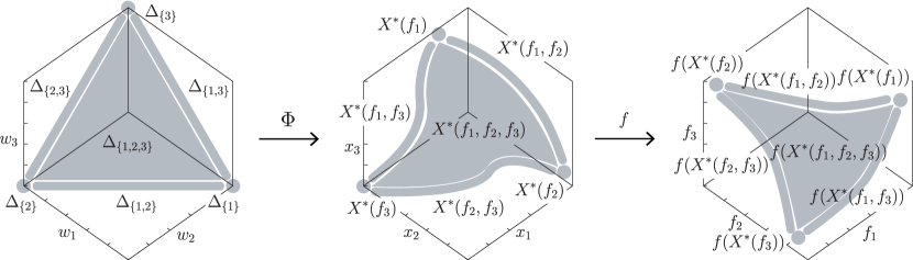
Figure 1. The Pareto set $X^{*}(f)$ (middle) and front $f(X^{*}(f))$ (right) of a simplicial problem $f=(f_{1},f_{2},f_{3})$. There exists a homeomorphism $\Phi$ from a simplex $\Delta^{2}$ to $X^{*}(f)$, sending each face to the Pareto set of a subproblem. The composite $f\circ\Phi:\Delta^{2}\to f(X^{*}(f))$ is also a homeomorphism.

Theorem 1.1.

Let $f:\mathbb{R}^{n}\to\mathbb{R}^{m}$ be a strongly convex $C^{r}$–mapping $(2\leq r\leq\infty)$. The multiobjective optimization problem minimizing $f$ is $C^{r-1}$–weakly simplicial. Furthermore, this problem is $C^{r-1}$–simplicial if the corank of the differential $df_{x}$ is equal to $1$ for any $x\in X^{*}(f)$.

For the definitions of strong convexity and weak simpliciality, see section 2. Under the assumptions of theorem 1.1, the weighted-sum scalarization gives an instance of the aforementioned homeomorphism $\Phi$, that is, the mapping $x^{*}:\Delta^{m-1}\to X^{*}(f)$ defined by

$$x^{*}(w)=\arg\min_{x\in\mathbb{R}^{n}}\left(\sum_{i=1}^{m}w_{i}f_{i}(x)\right)$$

is a homeomorphism. Since the scalarized function $\sum_{i=1}^{m}w_{i}f_{i}:\mathbb{R}^{n}\to\mathbb{R}$ is strongly convex (see section 2.3), the mapping $x^{*}$ is well-defined and can be efficiently computed by, e.g., gradient methods. By this property, scalarization-based subdivision methods [3, 17, 6, 23] are able to provide solutions for parametric-surface approximation methods in [12, 24] to build an approximation of $\Phi$.

Note that (strict) convexity of a mapping does not necessarily imply that the corresponding problem is simplicial. For example, the single objective problem minimizing the function $\exp(x)$ (defined on $\mathbb{R}$) does not have a Pareto solution (i.e. a minimizer), in particular it is not simplicial, although $\exp(x)$ is strictly convex.

As the example given in example 3.5 indicates, we cannot drop the assumption on the corank in theorem 1.1. Nevertheless, one can make any strongly convex mapping satisfy the corank assumption by a generic linear perturbation, provided that the dimension of the source is sufficiently larger than that of the target. See theorem 4.1 for details. We will further observe that theorem 4.1 would not hold without the assumption on the dimensions (cf. remark 4.4). Note that a small linear perturbation of a strongly convex problem does not cause substantial changes of the Pareto set (see remark 4.5 for details).

Applying theorem 1.1, we can show that several problems appearing in practical situations are simplicial. In 1967, Kuhn [13] showed that the Pareto set of a location problem under the Euclidean norm is the convex hull of demand points, which becomes a simplex when the demand points are in general position. We will observe in section 5 that this problem can be made strongly convex by suitable transformations on the target space preserving the Pareto ordering. In particular, our theorem gives an alternative proof of Kuhn’s result. Shoval et al. [22] proposed a multiobjective model for phenotypic divergence of species in evolutionary biology and indicated that its Pareto set is a curved simplex. Again, this problem becomes strongly convex after suitable transformations (see section 5). We can thus give a rigorous proof for the observation in [22].

The paper is organized as follows: After preliminaries in section 2, the proof of the main theorem will be given in section 3. In section 4, we will show that, under some assumption on the dimensions of the source and the target, any strongly convex problem becomes simplicial after a generic linear perturbation. Section 5 will be devoted to discussing practical problems.

2. Preliminaries

We introduce the definition of strongly convex problems and their properties and define $C^{r}$–(weakly) simplicial problems. Throughout the paper, we denote the index set $\Set{1,\dots,m}$ by $M$.

2.1. Multiobjective optimization

A multiobjective optimization problem is a problem minimizing objective functions $f_{1},\dots,f_{m}:X\to\mathbb{R}$ over a subset $X\subseteq\mathbb{R}^{n}$:

minimize $$f(x)=(f_{1}(x),\dots,f_{m}(x))$$

subject to $$x\in X(\subseteq\mathbb{R}^{n}).$$

According to the Pareto ordering, i.e.,

$$f(x)\prec f(y)\xLeftrightarrow{\text{def}}f_{i}(x)\leq f_{i}(y)\text{ for all }i\in M\text{ and }f_{j}(x)<f_{j}(y)\text{ for some }j\in M$$

we basically would like to obtain the Pareto set

$$X^{*}(f)=\Set{x\in X}{\forall y\in X,\ f(y)\not\prec f(x)}$$

and the Pareto front

$$f(X^{*}(f))=\Set{f(x)\in\mathbb{R}^{m}}{x\in X^{*}(f)}.$$

2.2. Simplicial problems

Here, we explain the definition of $C^{r}$–(weakly) simplicial problems for $0\leq r\leq\infty$. For $\varepsilon\geq 0$, we define the subset $\Delta_{\varepsilon}^{m-1}\varsubsetneq\mathbb{R}^{m}$ as follows:

$$\Delta_{\varepsilon}^{m-1}=\Set{(w_{1},\dots,w_{m})\in\mathbb{R}^{m}}{\sum_{i=1}^{m}w_{i}=1,\ w_{i}>-\varepsilon}\varsubsetneq\mathbb{R}^{m}.$$

Note that the closure $\overline{\Delta_{0}^{m-1}}$ is the standard simplex, which we will denote by

$$\Delta^{m-1}=\Set{(w_{1},\dots,w_{m})\in\mathbb{R}^{m}}{\sum_{i=1}^{m}w_{i}=1,\ w_{i}\geq 0}\varsubsetneq\mathbb{R}^{m}.$$

We also denote a face of $\Delta^{m-1}$ for $I\subseteq M$ by

$$\Delta_{I}=\Set{(w_{1},\dots,w_{m})\in\Delta^{m-1}}{w_{i}=0\ (i\not\in I)}\varsubsetneq\mathbb{R}^{m}.$$

For a subset $U\subseteq\mathbb{R}^{m}$, a continuous mapping $f:\Delta^{m-1}\to U$ is a $C^{r}$–mapping if there exist $\varepsilon>0$ and a $C^{r}$–mapping $\tilde{f}:\Delta^{m-1}_{\varepsilon}\to\mathbb{R}^{m}$ satisfying $\tilde{f}|_{\Delta^{m-1}}=f.$ A subspace $X\subseteq\mathbb{R}^{n}$ is $C^{r}$–diffeomorphic to the simplex $\Delta^{m-1}$ if there exist $\varepsilon>0$ and a $C^{r}$–immersion $\phi:\Delta_{\varepsilon}^{m-1}\to\mathbb{R}^{n}$ such that $\phi|_{\Delta^{m-1}}:\Delta^{m-1}\to X$ is a homeomorphism. The reader can refer to [15, §.2] for more general definition of diffeomorphisms between manifolds with corners.

Definition 2.1.

Let $X$ be a subset of $\mathbb{R}^{n}$ and $f=(f_{1},\dots,f_{m})$ be a mapping from $X$ to $\mathbb{R}^{m}$. For $I=\Set{i_{1},\dots,i_{k}}\subseteq M$ such that $i_{1}<\dots<i_{k}$, we put $f_{I}=(f_{i_{1}},\dots,f_{i_{k}})$. The problem minimizing $f$ is $C^{r}$–simplicial if there exists a $C^{r}$–mapping $\Phi:\Delta^{m-1}\to X^{*}(f)$ such that both of the restrictions $\Phi|_{\Delta_{I}}:\Delta_{I}\to X^{*}(f_{I})$ and $f|_{X^{*}(f_{I})}$ are $C^{r}$–diffeomorphisms for any $I\subseteq M$. The problem minimizing $f$ is $C^{r}$–weakly simplicial if there exists a $C^{r}$–mapping $\phi:\Delta^{m-1}\to f(X^{*}(f))$ satisfying $\phi(\Delta_{I})=f(X^{*}(f_{I}))$ for any $I\subseteq M$.

2.3. Pareto solutions of strongly convex mappings

In this subsection, a characterization of Pareto solutions of strongly convex $C^{1}$–mappings is given (see proposition 2.5). We begin this subsection with quickly reviewing the definition of (strong) convexity. A subset $X$ of $\mathbb{R}^{n}$ is convex if $tx+(1-t)y\in X$ for all $x,y\in X$ and all $t\in[0,1]$. Let $X$ be a convex set in $\mathbb{R}^{n}$. A function $f:X\to\mathbb{R}$ is convex if

$$f(tx+(1-t)y)\leq tf(x)+(1-t)f(y)$$

for all $x,y\in X$ and all $t\in[0,1]$. A function $f:X\to\mathbb{R}$ is strongly convex if there exists $\alpha>0$ such that

$$f(tx+(1-t)y)\leq tf(x)+(1-t)f(y)-\frac{1}{2}\alpha t(1-t)\left\|x-y\right\|^{2}$$

for all $x,y\in X$ and all $t\in[0,1]$, where $\left\|x-y\right\|$ denotes the Euclidean norm of $x-y$. A mapping $f=(f_{1},\dots,f_{m}):X\to\mathbb{R}^{m}$ is (strongly) convex if every $f_{i}$ is (strongly) convex. A problem minimizing a strongly convex mapping is called a strongly convex problem. The followings are basic properties of (strongly) convex mappings which will be needed later on:

Lemma 2.2 ([20, Theorem 2.1.2 (p. 54)]).

Let $X\subseteq\mathbb{R}^{n}$ be a convex open subset. A $C^{1}$–function $f:X\to\mathbb{R}$ is convex if and only if $f(x)+df_{x}\cdot(y-x)\leq f(y)$ for any $x,y\in X$.

Lemma 2.3 ([20, Theorem 2.1.11 (p. 65)]).

Let $X\subseteq\mathbb{R}^{n}$ be a convex open subset. A $C^{2}$–function $f:X\to\mathbb{R}$ is strongly convex if and only if there exists $\beta>0$ such that $m(f)_{x}\geq\beta$ for any $x\in X$, where $m(f)_{x}$ is the minimal eigenvalue of the Hessian matrix of $f$ at $x$.

Lemma 2.4 ([20, Theorem 2.2.6 (p. 85)]).

Let $f:\mathbb{R}^{n}\to\mathbb{R}$ be a strongly convex $C^{1}$–function. Then, there exists a unique point such that the function $f$ is minimized.

In the rest of this subsection we will prove the following proposition:

Proposition 2.5.

Let $f=(f_{1},\dots,f_{m}):\mathbb{R}^{n}\to\mathbb{R}^{m}$ be a strongly convex $C^{1}$–mapping. Then, $x\in X^{*}(f)$ if and only if there exists an element $(w_{1},\dots,w_{m})\in\Delta^{m-1}$ such that $f$ satisfies one (and hence both) of the following equivalent conditions:

1. $\sum_{i=1}^{m}w_{i}(df_{i})_{x}=0$.

2. The point $x\in\mathbb{R}^{n}$ is a unique element such that the function $\sum_{i=1}^{m}w_{i}f_{i}$ is minimized.

For the proof, we prepare some lemmas.

Lemma 2.6 ([16, Theorem 3.1.3 (p. 79)]).

Let $f=(f_{1},\dots,f_{m}):\mathbb{R}^{n}\to\mathbb{R}^{m}$ be a mapping and let $(w_{1},\dots,w_{m})\in\Delta^{m-1}$ be an element. If $x\in\mathbb{R}^{n}$ is a unique element such that the function $\sum_{i=1}^{m}w_{i}f_{i}$ is minimized, then $x\in X^{*}(f)$.

The following is a special case of the Karush-Kuhn-Tucker necessary condition for Pareto optimality.

Lemma 2.7 ([16, Theorem 3.1.5 (p. 39)]).

Let $f=(f_{1},\dots,f_{m}):\mathbb{R}^{n}\to\mathbb{R}^{m}$ be a $C^{1}$–mapping. If $x\in X^{*}(f)$, then there exists an element $(w_{1},\dots,w_{m})\in\Delta^{m-1}$ satisfying $\sum_{i=1}^{m}w_{i}(df_{i})_{x}=0$.

Lemma 2.8.

Let $f=(f_{1},\dots,f_{m}):\mathbb{R}^{n}\to\mathbb{R}^{m}$ be a convex $C^{1}$–mapping. Let $(w_{1},\dots,w_{m})\in\Delta^{m-1}$ be an element. Then, the following conditions for $x\in\mathbb{R}^{n}$ are equivalent.

1. $\sum_{i=1}^{m}w_{i}(df_{i})_{x}=0$.

2. The function $\sum_{i=1}^{m}w_{i}f_{i}:\mathbb{R}^{n}\to\mathbb{R}$ attains its minimum at $x$.

Proof of lemma 2.8.

Set $g=\sum_{i=1}^{m}w_{i}f_{i}$. Then, for any $x\in\mathbb{R}^{n}$, we have

(1) $$\sum_{i=1}^{m}w_{i}(df_{i})_{x}=dg_{x}.$$

Since $g$ is convex, we can deduce from lemma 2.2 that the following inequality holds for any $y\in\mathbb{R}^{n}$:

(2) $$g(x)+dg_{x}\cdot(y-x)\leq g(y).$$

Suppose that $\sum_{i=1}^{m}w_{i}(df_{i})_{x}=0$. We can easily deduce the assertion 2 from eq. 1 and eq. 2. Suppose that $\sum_{i=1}^{m}w_{i}f_{i}:\mathbb{R}^{n}\to\mathbb{R}$ attains its minimum at $x$. Since $dg_{x}$ is equal to $0$ and the equality eq. 1 holds, we have the assertion 1. ∎

Proof of proposition 2.5.

Suppose that $x\in X^{*}(f)$. Using lemma 2.7, we can verify that there exists an element $(w_{1},\dots,w_{m})\in\Delta^{m-1}$ satisfying $\sum_{i=1}^{m}w_{i}(df_{i})_{x}=0$. From lemma 2.8, the point $x\in\mathbb{R}^{n}$ is an element such that $\sum_{i=1}^{m}w_{i}f_{i}$ is minimized. Since $\sum_{i=1}^{m}w_{i}f_{i}$ is strongly convex $C^{1}$–function, by lemma 2.4, we have the assertion 2. Finally, suppose the assertion 2. Then, from lemma 2.6, we get $x\in X^{*}(f)$. ∎

2.4. Fold singularities

In this subsection we will briefly review the definition and basic properties of fold singularities (for details, see [5]). For $0\leq k\leq\min\Set{n,m}$, we define a subset $S_{k}\varsubsetneq J^{1}(\mathbb{R}^{n},\mathbb{R}^{m})$ as follows:

$$S_{k}=\Set{j^{1}g(x)\in J^{1}(\mathbb{R}^{n},\mathbb{R}^{m})}{\begin{minipage}[c]{159.33542pt} $x\in\mathbb{R}^{n}$, $g:\mathbb{R}^{n}\to\mathbb{R}^{m}$~{}:~{}$C^{2}$--mapping, $\min\Set{n,m}-\operatorname{rank}(dg_{x})=k$ \end{minipage}},$$

where $j^{1}g:\mathbb{R}^{n}\to J^{1}(\mathbb{R}^{n},\mathbb{R}^{m})$ is the $1$–jet extension of $g$. Let $g:\mathbb{R}^{n}\to\mathbb{R}^{m}$ be a $C^{2}$–mapping, $S\subseteq J^{1}(\mathbb{R}^{n},\mathbb{R}^{m})$ be a submanifold, and $x\in\mathbb{R}^{n}$. The mapping $j^{1}g$ is transverse to $S$ at $x$ if either of the following conditions holds:

• $j^{1}g(x)$ is not contained in $S$,

• $j^{1}g(x)\in S$ and $d(j^{1}g)_{x}(T_{x}\mathbb{R}^{n})+T_{j^{1}g(x)}S=T_{j^{1}g(x)}J^{1}(\mathbb{R}^{n},\mathbb{R}^{m})$.

The mapping $j^{1}g$ is transverse to $S$ if it is transverse to $S$ at any point in $\mathbb{R}^{n}$.

Suppose that $n$ is greater than or equal to $m$. For a $C^{2}$–mapping $f:\mathbb{R}^{n}\to\mathbb{R}^{m}$, we denote the critical point set of $f$ by $\mathrm{Crit}(f)\subseteq\mathbb{R}^{n}$. A point $x\in\mathrm{Crit}(f)$ is called a fold if the following conditions hold:

1. $j^{1}f$ is transverse to $S_{1}$ at $x_{0}$.

2. $T_{x_{0}}S_{1}(f)\oplus\ker df_{x_{0}}=T_{x_{0}}\mathbb{R}^{n}$, where $S_{1}(f)=(j^{1}f)^{-1}(S_{1})$.

Note that we can easily deduce from the condition 2 that the restriction $f|_{\mathrm{Crit}(f)}$ is an immersion around a fold.

Remark 2.9.

Let $f:\mathbb{R}^{n}\to\mathbb{R}^{m}$ be a $C^{\infty}$–mapping and $x\in\mathrm{Crit}(f)$ be a fold. One can take coordinate neighborhoods $(U,\varphi)$ and $(V,\psi)$ at $x$ and $f(x)$, respectively, so that they satisfy:

$$\psi\circ f\circ\varphi^{-1}(x_{1},\dots,x_{n})=\left(x_{1},\dots,x_{m-1},\sum_{k=m}^{n}\pm x_{k}^{2}\right).$$

In what follows we will give a useful criterion for detecting fold singularities. Let $f=(f_{1},\dots,f_{m}):\mathbb{R}^{n}\to\mathbb{R}^{m}$ be a $C^{2}$–mapping and $x_{0}\in\mathrm{Crit}(f)$. Suppose that the corank of $df_{x_{0}}$ is $1$ and the matrix $\left(\frac{\partial f_{i}}{\partial x_{j}}(x_{0})\right)_{1\leq i,j\leq m-1}$ is regular. We define the function $\lambda_{f}:\mathbb{R}^{n}\to\mathbb{R}^{n-m+1}$ as follows:

$$\lambda_{f}(x)=(J_{1}(x),\dots,J_{n-m+1}(x)),$$

where

$$J_{i}(x)=\det\begin{pmatrix}\dfrac{\partial f_{1}}{\partial x_{1}}(x)&\cdots&\dfrac{\partial f_{m}}{\partial x_{1}}(x)\\ \vdots&\ddots&\vdots\\ \dfrac{\partial f_{1}}{\partial x_{m-1}}(x)&\cdots&\dfrac{\partial f_{m}}{\partial x_{m-1}}(x)\\ \dfrac{\partial f_{1}}{\partial x_{m-1+i}}(x)&\cdots&\dfrac{\partial f_{m}}{\partial x_{m-1+i}}(x)\end{pmatrix}.$$

Lemma 2.10.

Under the situation above, $x_{0}$ is a fold if and only if the following conditions hold:

1. the differential $(d\lambda_{f})_{x_{0}}$ has rank $n-m+1$,

2. $\ker(d\lambda_{f})_{x_{0}}\oplus\ker df_{x_{0}}=T_{x_{0}}\mathbb{R}^{n}$.

Remark 2.11.

The two conditions in lemma 2.10 are equivalent to those in the original definition above. Indeed, the first condition is equivalent to the condition that $j^{1}f$ is transverse to $S_{1}$ at $x_{0}$, and $T_{x_{0}}S_{1}(f)$ is equal to $\ker(d\lambda_{f})_{x_{0}}$.

3. Proof of the main result

In this section we will show that strongly convex problems are simplicial. Let $f=(f_{1},\dots,f_{m}):\mathbb{R}^{n}\to\mathbb{R}^{m}$ be a strongly convex $C^{r}$–mapping $(2\leq r\leq\infty)$. Since $\sum_{i=1}^{m}w_{i}f_{i}$ is strongly convex for any $(w_{1},\dots,w_{m})\in\Delta^{m-1}$, there exists a unique point $x\in\mathbb{R}^{n}$ such that $\sum_{i=1}^{m}w_{i}f_{i}$ is minimized (see lemma 2.4). We denote this minimizing point by $\arg\min_{x\in\mathbb{R}^{n}}\left(\sum_{i=1}^{m}w_{i}f_{i}(x)\right)\in\mathbb{R}^{n}$, which is contained in $X^{*}(f)$ by lemma 2.6. We can thus define a mapping $x^{*}:\Delta^{m-1}\to X^{*}(f)$ as follows:

$$x^{*}(w)=\arg\min_{x\in\mathbb{R}^{n}}\left(\sum_{i=1}^{m}w_{i}f_{i}(x)\right).$$

Theorem 3.1.

Let $f=(f_{1},\dots,f_{m}):\mathbb{R}^{n}\to\mathbb{R}^{m}$ be a strongly convex $C^{r}$–mapping $(2\leq r\leq\infty)$.

1. The mapping $x^{*}:\Delta^{m-1}\to X^{*}(f)$ (and thus $f\circ x^{*}:\Delta^{m-1}\to f(X^{*}(f))$) is a surjective mapping of class $C^{r-1}$.

2. Suppose that the corank of $df_{x}$ is equal to $1$ for any $x\in X^{*}(f)$.

   1. The mapping $x^{*}:\Delta^{m-1}\to X^{*}(f)$ is a $C^{r-1}$–diffeomorphism.

   2. The restriction $f|_{X^{*}(f)}:X^{*}(f)\to\mathbb{R}^{m}$ is a $C^{r-1}$–embedding.

Note that this theorem obviously holds for $m=1$. For this reason, in the rest of this section we will assume $m\geq 2$.

theorem 1.1 follows from this theorem as follows: It is easy to see that any subproblem of a strongly convex problem is again strongly convex. In particular, by applying theorem 3.1 to each subproblem, we can show that the image of the restriction $x^{*}$ on $\Delta_{I}$ is equal to $X^{*}(f_{I})$ for any $I\subseteq M$. Thus a strongly convex problem is weakly simplicial. We can further deduce from the assertion 2 of theorem 3.1 that a strongly convex problem is simplicial under the assumption on the coranks of differentials.

Remark 3.2.

The corank assumption in 2 implies that $n$ is greater than or equal to $m-1$. As we will show in the proof, under this assumption any point in $X^{*}(f)$ for a mapping $f$ is a fold if $n\geq m$.

Remark 3.3.

In general, the mapping $x^{*}$ for a strongly convex problem (without the corank assumption) is not necessarily a diffeomorphism. We will give an explicit example of such a problem with a non-injective $x^{*}$ in example 3.4.

Proof of 1 in theorem 3.1.

First of all, we can immediately deduce from proposition 2.5 that $x^{*}$ is surjective. Let $\delta^{\prime}>0$ be a positive number and $g:\Delta_{\delta^{\prime}}^{m-1}\times\mathbb{R}^{n}\to\mathbb{R}^{n}$ be a $C^{r-1}$–mapping defined by $g(w,x)=\sum_{k=1}^{m}w_{k}(df_{k})_{x}$. We can easily deduce from lemma 2.8 that $x^{*}$ is an implicit function of the equation $g(w,x)=0$ defined on $\Delta^{m-1}$. Differentiating $g$, we have $\frac{\partial g_{i}}{\partial x_{j}}=\sum_{k=1}^{m}w_{k}\frac{\partial f_{k}}{\partial x_{i}\partial x_{j}}$. Thus the matrix $\left(\frac{\partial g_{i}}{\partial x_{j}}\right)_{1\leq i,j\leq n}$ is equal to $\sum_{k=1}^{m}w_{k}H(f_{k})_{x}$, where $H(f_{k})_{x}$ is the Hessian matrix of $f_{k}$ at $x$. Since $f_{k}$ is strongly convex, the Hessian matrix $H(f_{k})_{x}$ is positive definite (see lemma 2.3). Thus, the matrix $\left(\frac{\partial g_{i}}{\partial x_{j}}\right)_{1\leq i,j\leq n}$ is regular on $\Delta^{m-1}$. By the implicit function theorem, for any $y\in\Delta^{m-1}$ there exists an open neighborhood $U_{y}\subseteq\Delta_{\delta^{\prime}}^{m-1}$ and a (unique) $C^{r-1}$–mapping $x^{*}_{y}:U_{y}\to\mathbb{R}^{n}$ such that $x^{*}_{y}(y)=x^{*}(y)$ and $g(w,x^{*}_{y}(w))=0$ for any $w\in U_{y}$. We can further deduce from uniqueness of an implicit function that $x^{*}_{y}$ coincides with $x^{*}_{y^{\prime}}$ on $U_{y}\cap U_{y^{\prime}}$ for distinct $y,y^{\prime}\in\Delta^{m-1}$. Since $U=\bigcup_{y\in\Delta^{m-1}}U_{y}$ is an open neighborhood of $\Delta^{m-1}$, one can take $\delta<\delta^{\prime}$ so that $\Delta^{m-1}_{\delta}$ is contained in $U$. We can define $\widetilde{x^{*}}:\Delta_{\delta}^{m-1}\to\mathbb{R}^{n}$ by $\widetilde{x^{*}}(w)=x^{*}_{y}(w)$ for $w\in U_{y}$. It is easy to see that $\widetilde{x^{*}}$ is a $C^{r-1}$–mapping and is an extension of $x^{*}$. Thus $x^{*}$ is a $C^{r-1}$–mapping. ∎

Proof of 2.A in theorem 3.1.

For $\varepsilon\geq 0$, we define a subset $D^{m-1}_{\varepsilon}\varsubsetneq\mathbb{R}^{m-1}$ by

$$D^{m-1}_{\varepsilon}=\Set{(z_{1},\dots,z_{m-1})\in\mathbb{R}^{m-1}}{\sum_{i}z_{i}<1+\varepsilon,\hskip 3.00003ptz_{i}>-\varepsilon}.$$

We denote the closure $\overline{D_{0}^{m-1}}$ by $D^{m-1}$. It is easy to check that the projection $p:\Delta_{\varepsilon}^{m-1}\to D_{\varepsilon}^{m-1}$ defined by $p(w_{1},\dots,w_{m})=(w_{1},\dots,w_{m-1})$ is a diffeomorphism. In what follows we will identify $\Delta_{\varepsilon}^{m-1}$ with $D_{\varepsilon}^{m-1}$ by $p$.

Since $\widetilde{x^{*}}$ constructed in the proof above is an implicit function of the equation $g(w,x)=0$, the following equality holds:

$$0=\sum_{k=1}^{m}w_{k}(df_{k})_{\widetilde{x^{*}}(w)}=\sum_{k=1}^{m-1}z_{k}(df_{k})_{\widetilde{x^{*}}(z)}+\left(1-\sum_{k=1}^{m-1}z_{k}\right)(df_{m})_{\widetilde{x^{*}}(z)},$$

where $(z_{1},\dots,z_{m-1})\in D_{\delta}^{m-1}$ is a point corresponding to $w\in\Delta^{m-1}_{\delta}$. Differentiating the both sides of the equation above by $z_{j}$ $(j=1,\dots,m-1)$, we obtain the following equality:

$$0= \sum_{k=1}^{m-1}z_{k}\left(H(f_{k})_{\widetilde{x^{*}}(z)}\frac{\partial\widetilde{x^{*}}}{\partial z_{j}}\right)+(df_{j})_{\widetilde{x^{*}}(z)}$$

$$+\left(1-\sum_{k=1}^{m-1}z_{k}\right)\left(H(f_{m})_{\widetilde{x^{*}}(z)}\frac{\partial\widetilde{x^{*}}}{\partial z_{j}}\right)-(df_{m})_{\widetilde{x^{*}}(z)}.$$

We thus obtain:

$$\frac{\partial\widetilde{x^{*}}}{\partial z_{j}} =-\left(\sum_{k=1}^{m-1}z_{k}H(f_{k})_{\widetilde{x^{*}}(z)}+\left(1-\sum_{k=1}^{m-1}z_{k}\right)H(f_{m})_{\widetilde{x^{*}}(z)}\right)^{-1}\left((df_{j})_{\widetilde{x^{*}}(z)}-(df_{m})_{\widetilde{x^{*}}(z)}\right)$$

$$=-A(z)\left((df_{j})_{\widetilde{x^{*}}(z)}-(df_{m})_{\widetilde{x^{*}}(z)}\right),$$

where we denote the matrix $\left(\sum_{k=1}^{m-1}z_{k}H(f_{k})_{\widetilde{x^{*}}(z)}+\left(1-\sum_{k=1}^{m-1}z_{k}\right)H(f_{m})_{\widetilde{x^{*}}(z)}\right)^{-1}$ by $A(z)$, which is positive definite for $z\in D^{m-1}$. Since $D^{m-1}$ is compact and the corank of $df_{\widetilde{x^{*}}(z)}$ is equal to $1$ for any $z\in D^{m-1}$, by retaking $\delta$ if necessary, we can assume that the corank of $df_{\widetilde{x^{*}}(z)}$ is equal to $1$ and $A(z)$ is positive definite, and thus regular, for any $z\in D_{\delta}^{m-1}$. (Note that the condition $\operatorname{corank}(df_{x})=1$ is an open condition in $\mathrm{Crit}(f)$.)

We will show that the matrix

(3) $$\begin{pmatrix}(df_{1})_{\widetilde{x^{*}}(z)}-(df_{m})_{\widetilde{x^{*}}(z)}&\cdots&(df_{m-1})_{\widetilde{x^{*}}(z)}-(df_{m})_{\widetilde{x^{*}}(z)}\end{pmatrix}$$

has rank $m-1$ for any $z\in D^{m-1}$. If not so, there exists $a_{i}\in\mathbb{R}$ with $(a_{1},\dots,a_{m-1})\neq 0$ such that

$$\sum_{i=1}^{m-1}a_{i}\left((df_{i})_{\widetilde{x^{*}}(z)}-(df_{m})_{\widetilde{x^{*}}(z)}\right)=0.$$

On the other hand, by the definition of $\widetilde{x^{*}}$, we obtain

$$\sum_{j=1}^{m-1}z_{j}(df_{j})_{\widetilde{x^{*}}(z)}+\left(1-\sum_{i=1}^{m-1}z_{i}\right)(df_{m})_{\widetilde{x^{*}}(z)}=0.$$

Thus, two vectors $\left(z_{1},\dots,z_{m-1},1-\sum_{i=1}^{m-1}z_{i}\right)$ and $\left(a_{1},\dots,a_{m-1},-\sum_{i=1}^{m-1}a_{i}\right)$ are contained in $\ker df_{\widetilde{x^{*}}(z)}$. However, these are linearly independent and contradict the assumption $\operatorname{corank}\left(df_{\widetilde{x^{*}}(z)}\right)=1$. Therefore, the matrix in eq. 3 has rank $m-1$ for any $z\in D^{m-1}$. Since the condition that the matrix in eq. 3 has rank $m-1$ is an open condition for $z$, we can assume that this condition holds for any $D_{\delta}^{m-1}$ by making $\delta$ sufficiently small. The differential

$$d\widetilde{x^{*}}_{z}=-A(z)\left((df_{1})_{\widetilde{x^{*}}(z)}-(df_{m})_{\widetilde{x^{*}}(z)},\dots,(df_{m-1})_{\widetilde{x^{*}}(z)}-(df_{m})_{\widetilde{x^{*}}(z)}\right)$$

also has rank $m-1$ since $A(z)$ is regular for any $z\in D_{\delta}^{m-1}$.

We next show that the mapping $x^{*}$ is injective. Assume that $x^{*}(w)$ is equal to $x^{*}(w^{\prime})$ for $w,w^{\prime}\in\Delta^{m-1}$. Since the corank of $df_{x^{*}(w)}$ is $1$ and $\sum_{j=1}^{m}w_{j}(df_{j})_{x^{*}(w)}=0$, we can obtain $\operatorname{Im}(df_{x^{*}(w)})=\left\langle w\right\rangle^{\perp}$. In the same way, we can also prove that $\operatorname{Im}(df_{x^{*}(w^{\prime})})$ is equal to $\left\langle w^{\prime}\right\rangle^{\perp}$. From the assumption, we can deduce that $\left\langle w\right\rangle^{\perp}$ is equal to $\left\langle w^{\prime}\right\rangle^{\perp}$ and thus $w=w^{\prime}$.

We have shown that $x^{*}$ is an injective immersion. Since $\Delta^{m-1}$ is compact, $x^{*}$ is a homeomorphism and thus a diffeomorphism to its image, which is equal to $X^{*}(f)$. ∎

Proof of 2.B in theorem 3.1.

We first prove that $f|_{X^{*}(f)}$ is injective. Let $w,z\in\Delta^{m-1}$, $x=x^{*}(w)$ and $y=x^{*}(z)$. Suppose that $f(x)$ is equal to $f(y)$. Then $\left(\sum_{i=1}^{m}w_{i}f_{i}\right)(x)$ is also equal to $\left(\sum_{i=1}^{m}w_{i}f_{i}\right)(y)$. Since the function $\sum_{i=1}^{m}w_{i}f_{i}$ is strongly convex, the point minimizing $\sum_{i=1}^{m}w_{i}f_{i}$ is unique (see lemma 2.4). Thus, $x$ is equal to $y$.

As we noted in remark 3.2, the corank assumption implies that $n$ is greater than or equal to $m-1$. If $n=m-1$, this assumption further implies that $f$ is an immersion at any point in $X^{*}(f)$. The restriction $f|_{X^{*}(f)}$ is thus an embedding since any injective immersion on a compact manifold is an embedding. In what follows we will assume $n\geq m$.

We next show that any point $x\in X^{*}(f)$ is a fold of $f$. The following transformations preserve strong convexity of $f$:

• $(f_{1},\dots,f_{m})\mapsto(f_{\sigma(1)},\dots,f_{\sigma(m)})\quad(\sigma\in\mathfrak{S}_{m})$,

• $(f_{1},\dots,f_{m})\mapsto(f_{1},\dots,f_{m}+\alpha f_{i})\quad(\alpha>0,i=1,\dots,m-1)$, and

• linear transformations of the source of $f$,

where $\mathfrak{S}_{m}$ is the symmetric group of degree $m$. By applying these transformations if necessary, we can assume the followings:

$$(df_{m})_{x}=0,\quad\left(\frac{\partial f_{i}}{\partial x_{j}}(x)\right)_{1\leq i,j\leq m-1}=I_{m-1},\quad\frac{\partial f_{i}}{\partial x_{j}}(x)=0\ \begin{pmatrix}i=1,\dots,m\\ j=m,\dots,n\end{pmatrix}.$$

Let $\lambda_{f}:\mathbb{R}^{n}\to\mathbb{R}^{n-m+1}$ be the mapping defined in section 2.4. By lemma 2.10, it suffices to show the followings:

1. the rank of $(d\lambda_{f})_{x}$ is $n-m+1$,

2. $\ker(d\lambda_{f})_{x}\oplus\ker df_{x}=T_{x}\mathbb{R}^{n}$.

By the assumptions above, we can calculate $(d\lambda_{f})_{x}$ as follows:

$$(d\lambda_{f})_{x} =\pm\left(\dfrac{\partial^{2}f_{m}}{\partial x_{j}\partial x_{m-1+i}}(x)\right)_{1\leq i\leq n-m+1,1\leq j\leq n}$$

$$=\pm\left(\begin{array}[]{c|c}\text{\rule{0.0pt}{15.0pt} \Large{0}}_{(n-m+1)\times(m-1)}&\emph{\Large{I}}_{n-m+1}\end{array}\right)H(f_{m})_{x}.$$

Since $f_{m}$ is strongly convex, the Hessian matrix $H(f_{m})_{x}$ is positive definite, in particular regular by lemma 2.3. Thus, the condition (A) holds. The above calculation also implies the following equality:

$$\ker(d\lambda_{f})_{x}=\left\langle H(f_{m})_{x}^{-1}e_{1},\dots,H(f_{m})_{x}^{-1}e_{m-1}\right\rangle.$$

Let $v\in\ker(d\lambda_{f})_{x}\cap\ker(df)_{x}$. From the equality above, we can find $w\in\mathbb{R}^{m-1}\times\Set{0}\varsubsetneq\mathbb{R}^{m}$ such that $v=H(f_{m})_{x}^{-1}w$. Thus the following holds:

$$0=df_{x}(v)=\begin{pmatrix}I_{m-1}&0\\ 0&0\end{pmatrix}H(f_{m})_{x}^{-1}w.$$

We can deduce the following from this equality:

$${}^{t}wH(f_{m})^{-1}_{x}w=0.$$

Since $H(f_{m})$ is positive definite by lemma 2.3, $w$ is equal to $0$. Since the corank of $df_{x}$ is equal to $1$, we can deduce the following from the condition (A):

$$\dim\ker(d\lambda_{f})_{x}+\dim\ker(df_{x})=n.$$

Thus the condition (B) also holds. We can eventually conclude that $f|_{X^{*}(f)}$ is an immersion. ∎

3.1. Examples

One of the most simple and representative instances of strongly convex problem is the multiobjective location problem under the Euclidean norm. It is well known that the Pareto set (resp. the Pareto front) of this problem is a convex hull of minimizing points (resp. their values) of individual objective functions [13]. Thus, if these minimizing points are in general position, then the convex hull becomes a simplex and this problem is a $C^{0}$–simplicial problem.

In this section we will show that in the strongly convex case, the condition that minimizing points are in general position is no longer necessary nor sufficient to ensure $C^{r}$–simpliciality, and the corank assumption is still essential to determine the topology of the Pareto set and the Pareto front. To this end, we will give two examples of strongly convex mappings from $\mathbb{R}^{3}$ to $\mathbb{R}^{3}$, and discuss the configurations of Pareto sets of them. As we mentioned in the beginning of section 3, for any strongly convex mapping $f:\mathbb{R}^{3}\to\mathbb{R}^{3}$ we can define a mapping $x^{*}:\Delta^{2}\to X^{*}(f)$. The first example (given in example 3.4) has a corank $2$ differential at a point in the Pareto set, and the corresponding $x^{*}$ is not a diffeomorphism (despite the fact that the minimizing points of the three component functions are in general position). This example implies that we cannot drop the corank assumption in the assertion 2 of theorem 3.1. The second example (given in example 3.5) satisfies the corank assumption, and thus the corresponding $x^{*}$ is a diffeomorphism (although the minimizing points of the three component functions are not in general position).

Example 3.4 (general position with corank $2$).

Define a mapping $f=(f_{1},f_{2},f_{3}):\mathbb{R}^{3}\to\mathbb{R}^{3}$ as follows:

$$f_{1}(x,y,z) =x^{2}+y^{2}+z^{2},$$

$$f_{2}(x,y,z) =x+y+x^{2}+y^{2}+z^{2},$$

$$f_{3}(x,y,z) =-(x+y)+x^{2}+2y^{2}+z^{2}.$$

The mapping $f$ is strongly convex. We will check that $X^{*}(f)$ contains a singularity of corank $2$, and is not diffeomorphic to $\Delta^{2}$. The differentials at $p=(x,y,z)\in\mathbb{R}^{3}$ are

$$df_{1,p} =(2x,2y,2z)$$

$$df_{2,p} =(1+2x,1+2y,2z)$$

$$df_{3,p} =(-1+2x,-1+4y,2z),$$

and thus the corank of $df_{\boldsymbol{0}}$ is $2$. Since $f$ is strongly convex, the mapping $x^{*}:\Delta^{2}\to X^{*}(f)$ is surjective by the assertion 1 of theorem 3.1. Regarding $\Delta^{2}$ as $D^{2}=\Set{(w_{2},w_{3})}{w_{2},w_{3}\geq 0,w_{2}+w_{3}\leq 1}$, we obtain

$$x^{*}(w_{2},w_{3})=\left(-\frac{w_{2}-w_{3}}{2},-\frac{w_{2}-w_{3}}{2(1+w_{3})},0\right).$$

Obviously $x^{*}$ maps the line defined by $w_{2}-w_{3}=0$ in $\Delta^{2}=D^{2}$ into single point (the origin), while it is injective at points outside the above line. Thus $X^{*}(f)(=x^{*}(\Delta^{2}))$ is not diffeomorphic to $\Delta^{2}$. Figure 2 describes the Pareto set of $f$, together with the contours of the functions $f_{1}$ (red), $f_{2}$ (blue) and $f_{3}$ (green).

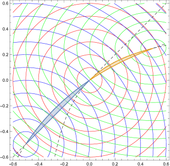
Figure 2. The Pareto set of $f$. The union of two domains colored with orange and blue is the Pareto set.

For $\varepsilon\in\mathbb{R}-\Set{0}$, we define another mapping $h_{\varepsilon}:\mathbb{R}^{3}\to\mathbb{R}^{3}$ as follows:

$$h_{\varepsilon}(x,y,z)=(f_{1}(x,y,z)+\varepsilon z,f_{2}(x,y,z),f_{3}(x,y,z)).$$

Note that the mapping $h_{\varepsilon}$ is a linear perturbation of $f$. It is easy to verify that the mapping $h_{\varepsilon}$ is strongly convex and never has corank $2$ critical points. Thus the problem minimizing $h_{\varepsilon}$ is simplicial. We will see in section 4 that in general any strongly convex problem becomes simplicial after a generic linear perturbation (see theorem 4.1).

Example 3.5 (non-general position without corank $2$).

We define a mapping $f=(f_{1},f_{2},f_{3}):\mathbb{R}^{3}\to\mathbb{R}^{3}$ as follows:

$$f_{1}(x,y,z) =x^{2}+(-y+x)^{2}+z^{2},$$

$$f_{2}(x,y,z) =2(x-1)^{2}+(-y+x-1)^{2}+z^{2},$$

$$f_{3}(x,y,z) =(x-2)^{2}+(y+x-2)^{2}+z^{2}.$$

The mapping $f$ is strongly convex. We will check that $f$ satisfies the assumption in the assertion 2 of theorem 3.1 (although the minimizing points of $f_{1},f_{2},f_{3}$ are not in general position). Let $p=(x,y,z)$ be a point in $X^{*}(f)$. It is easy to see that $z$ is equal to $0$. Thus the differentials at $p$ are calculated as follows:

$$\left(df_{1}\right)_{p} =(4x-2y,-2x+2y,0),$$

$$\left(df_{2}\right)_{p} =(6x-2y-6,-2x+2y+2,0),$$

$$\left(df_{3}\right)_{p} =(4x+2y-8,2x+2y-4,0).$$

Suppose that the corank of $df_{p}$ is greater than or equal to $2$. Then the following equalities hold:

(4) $$0=\det\begin{pmatrix}4x-2y&-2x+2y\\ 6x-2y-6&-2x+2y+2\end{pmatrix}=4\left(x-\frac{y}{2}-\frac{1}{2}\right)^{2}-\left(y-3\right)^{2}+8,$$

(5) $$0=\det\begin{pmatrix}4x-2y&-2x+2y\\ 4x+2y-8&2x+2y-4\end{pmatrix}=2\left(8\left(x-1\right)^{2}-4\left(y-\frac{3}{2}\right)^{2}+1\right).$$

These equalities give rise to two hyperbolas given in fig. 3(a) (the red hyperbola is defined by eq. 4, while the blue one is defined by eq. 5). As shown in fig. 3(a), the two hyperbolas intersect at two points. One is the origin $\boldsymbol{0}$ and let $q=(x^{\prime},y^{\prime})$ be the other. Since the rank of $\left((df_{1})_{\boldsymbol{0}},(df_{2})_{\boldsymbol{0}},(df_{3})_{\boldsymbol{0}}\right)$ is $2$, $(x,y)$ is not equal to $(0,0)$. Thus we obtain $(x,y)=(x^{\prime},y^{\prime})$. However, since $y^{\prime}-x^{\prime}>1$ and $x^{\prime},y^{\prime}>1$, all of the three values $-2x^{\prime}+2y^{\prime},-2x^{\prime}+2y^{\prime}+2$ and $2x^{\prime}+2y^{\prime}-4$ are greater than $0$, contradicting proposition 2.5. Hence we can conclude that there is no point $p\in X^{*}(f)$ with $\operatorname{corank}(df_{p})\geq 2$. Figure 3(b) describes the Pareto set of $f$, together with the contours of the functions $f_{1}$ (red), $f_{2}$ (blue) and $f_{3}$ (green).

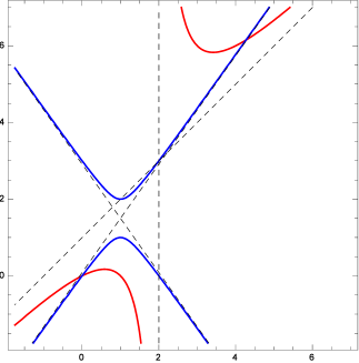
(a) Two hyperbolas.

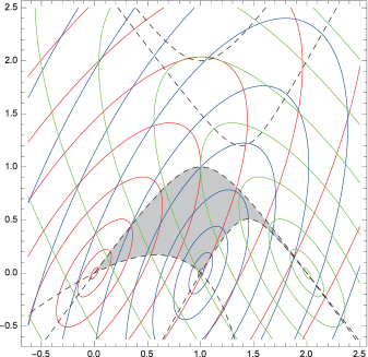
(b) The Pareto set of $f$ (projected on the $xy$–plane).

Figure 3. The dotted lines in fig. 3(a) are asymptotes of the hyperbolas.

4. Generic linear perturbations of strongly convex mappings

In this section, we will investigate the multiobjective optimization problem minimizing a generically linearly perturbed strongly convex mapping. Let $\mathcal{L}(\mathbb{R}^{n},\mathbb{R}^{m})$ be the space consisting of all linear mappings from $\mathbb{R}^{n}$ into $\mathbb{R}^{m}$. In what follows we will regard $\mathcal{L}(\mathbb{R}^{n},\mathbb{R}^{m})$ as the Euclidean space $(\mathbb{R}^{n})^{m}$ in the obvious way. The purpose of this section is to show the following theorem:

Theorem 4.1.

Let $f:\mathbb{R}^{n}\to\mathbb{R}^{m}$ $(n\geq m)$ be a strongly convex $C^{r}$–mapping $(2\leq r\leq\infty)$. If $n-2m+4>0$, then there exists a subset $\Sigma\varsubsetneq\mathcal{L}(\mathbb{R}^{n},\mathbb{R}^{m})$ with Lebesgue measure zero such that for any $\pi\in\mathcal{L}(\mathbb{R}^{n},\mathbb{R}^{m})-\Sigma$ the mapping $f+\pi$ never has differential with corank greater than $1$ on its Pareto set. In particular, the multiobjective optimization problem minimizing $f+\pi:\mathbb{R}^{n}\to\mathbb{R}^{m}$ is $C^{r-1}$–simplicial.

We begin with observing that strong convexity is preserved under linear perturbations.

Lemma 4.2.

Let $f:\mathbb{R}^{n}\to\mathbb{R}^{m}$ be a strongly convex mapping. Then, for any $\pi\in\mathcal{L}(\mathbb{R}^{n},\mathbb{R}^{m})$, the mapping $f+\pi:\mathbb{R}^{n}\to\mathbb{R}^{m}$ is also a strongly convex mapping.

Proof of lemma 4.2.

Obviously, it is sufficient to show the statement under the assumption that $f$ is a function (i.e. $m=1$). For $x,y\in\mathbb{R}^{n}$ and $t\in[0,1]$, the following holds:

$$t\left((f+\pi)(x)\right)+(1-t)\left((f+\pi)(y)\right)-(f+\pi)(tx+(1-t)y)$$

$$=t\left(f(x)+\pi(x)\right)+(1-t)\left(f(y)+\pi(y)\right)-f(tx+(1-t)y)-\pi(tx+(1-t)y)$$

$$=tf(x)+(1-t)f(y)-f(tx+(1-t)y),$$

where the last equality holds since $\pi$ is linear. Since $f$ is strongly convex, there exists $\alpha>0$ satisfying the following inequality for any $x,y\in\mathbb{R}^{n}$ and $t\in[0,1]$:

$$tf(x)+(1-t)f(y)-f(tx+(1-t)y)\geq\frac{1}{2}\alpha t(1-t)\left\|x-y\right\|^{2}.$$

Hence, the mapping $f+\pi$ is also strongly convex. ∎

Before proving theorem 4.1, we will briefly review the result in [10] needed here. Let $S_{k}\varsubsetneq J^{1}(\mathbb{R}^{n},\mathbb{R}^{m})$ be the subset defined in section 2.4. It is known that $S_{k}$ is a submanifold of $J^{1}(\mathbb{R}^{n},\mathbb{R}^{m})$ satisfying the following (see [5]):

$$\operatorname{codim}S_{k}=(n-v+k)(m-v+k)$$

where $\operatorname{codim}S_{k}=\dim J^{1}(\mathbb{R}^{n},\mathbb{R}^{m})-\dim S_{k}$ and $v=\min\Set{n,m}$. The following lemma is merely a special case of [10, Theorem 1]:

Lemma 4.3 (cf. [10]).

Let $f:\mathbb{R}^{n}\to\mathbb{R}^{m}$ be a $C^{r}$–mapping. Let $k$ be an integer satisfying $1\leq k\leq\min\Set{n,m}$. If $r>\max\Set{n-\operatorname{codim}S_{k},0}+1$, then there exists a subset $\Sigma\varsubsetneq\mathcal{L}(\mathbb{R}^{n},\mathbb{R}^{m})$ with Lebesgue measure zero such that for any $\pi\in\mathcal{L}(\mathbb{R}^{n},\mathbb{R}^{m})-\Sigma$, the mapping $j^{1}(f+\pi):\mathbb{R}^{n}\to J^{1}(\mathbb{R}^{n},\mathbb{R}^{m})$ is transverse to $S_{k}$.

Proof of theorem 4.1.

In the case $m=1$, it is clearly seen that theorem 4.1 holds. Hence, we will consider the case $m\geq 2$. Since $n\geq m$, the codimension of $S_{2}$ is equal to $2(n-m+2)$. By the assumption $n-2m+4>0$, we can obtain the inequality $\operatorname{codim}S_{2}>n$. Let $k$ be an integer with $2\leq k\leq m$. It follows that

$$n-\operatorname{codim}S_{k}\leq n-\operatorname{codim}S_{2}<0.$$

In particular, for a mapping $g:\mathbb{R}^{n}\to\mathbb{R}^{m}$, transversality of $j^{1}g$ to $S_{k}$ is equivalent to the condition that $j^{1}g(\mathbb{R}^{n})\cap S_{k}=\emptyset$, that is, $g$ has no corank $k$ critical points (see [5, Ch. II, Proposition 4.2]). Furthermore, the following inequality holds:

$$r\geq 2>\max\Set{n-\operatorname{codim}S_{k},0}+1.$$

We can deduce from lemma 4.3, together with the observations above, that there exists $\Sigma_{k}\varsubsetneq\mathcal{L}(\mathbb{R}^{n},\mathbb{R}^{m})$ with Lebesgue measure zero such that the mapping $f+\pi$ has no corank $k$ critical points for any $\pi\in\mathcal{L}(\mathbb{R}^{n},\mathbb{R}^{m})-\Sigma_{k}$. Set $\Sigma=\bigcup_{l=2}^{m}\Sigma_{l}\varsubsetneq\mathcal{L}(\mathbb{R}^{n},\mathbb{R}^{m})$, which also has Lebesgue measure zero. Lastly, we can easily verify that $\Sigma$ satisfies the conditions in theorem 4.1. ∎

Remark 4.4.

We cannot drop the assumption $n-2m+4>0$ in theorem 4.1. Let $G(x)=\left(g_{1}(x)-x_{3},g_{2}(x)-x_{4},g_{1}(x)+x_{3},g_{2}(x)+x_{4}\right)$ be a map from $\mathbb{R}^{4}$ to $\mathbb{R}^{4}$, where

$$g_{1}(x) =x_{1}^{2}+x_{3}x_{2}+\frac{1}{2}\left(x_{2}^{2}+x_{4}x_{1}\right)+x_{3}^{2}+x_{4}^{2},$$

$$g_{2}(x) =x_{2}^{2}+x_{4}x_{1}+\frac{1}{2}\left(x_{1}^{2}+x_{3}x_{2}\right)+x_{3}^{2}+x_{4}^{2}.$$

The mapping $G$ is strongly convex and has a corank $2$ critical point at the origin. In what follows, we will see that the Pareto set of any small linear perturbation of $G$ contains a corank $2$ critical point. (Note that the inequality $n-2m+4>0$ does not hold when $n=m=4$.)

The Jacobi matrix of $G$ at the origin is $dG_{0}=\left(\begin{smallmatrix}O&O\\ -I&I\end{smallmatrix}\right)$, where $I$ and $O$ are $2\times 2$ unit matrix and zero matrix, respectively. Define the cokernel of $dG_{0}$ as

$$\operatorname{coker}dG_{0}=\Set{\left(v_{1},v_{2},v_{3},v_{4}\right)\in\mathbb{R}^{4}}{\sum_{i=1}^{4}v_{i}\left(dG_{i}\right)_{0}=0},$$

then, the subspace $\operatorname{coker}dG_{0}$ is equal to $\left\langle(1,0,1,0),\ (0,1,0,1)\right\rangle$. In particular, the subspace $\operatorname{coker}dG_{0}$ intersects with the interior of $\Delta^{3}$.

For $(x,\pi)\in\mathbb{R}^{4}\times\mathcal{L}(\mathbb{R}^{4},\mathbb{R}^{4})$, put $d(G+\pi)_{x}=\left(\begin{smallmatrix}A(x,\pi)&B(x,\pi)\\ C(x,\pi)&D(x,\pi)\end{smallmatrix}\right)$ where $A(x,\pi)$, $B(x,\pi)$, $C(x,\pi)$, and $D(x,\pi)$ are $2\times 2$ matrices. We can take an open neighborhood $U$ of $(0,0)\in\mathbb{R}^{4}\times\mathcal{L}(\mathbb{R}^{4},\mathbb{R}^{4})$ so that the matrix $D(x,\pi)$ is invertible for any $(x,\pi)\in U$. By multiplying the matrix $\left(\begin{smallmatrix}I&O\\ -D^{-1}(x,\pi)C(x,\pi)&I\end{smallmatrix}\right)$ to $d(G+\pi)_{x}$ from the right, we obtain the matrix $\left(\begin{smallmatrix}A(x,\pi)-B(x,\pi)D^{-1}(x,\pi)C(x,\pi)&B(x,\pi)\\ O&D(x,\pi)\end{smallmatrix}\right)$. Put $E(x,\pi)=A(x,\pi)-B(x,\pi)D^{-1}(x,\pi)C(x,\pi)$. The matrix $E(0,0)$ is the zero matrix, and

$$\left.\frac{\partial E(x,\pi)}{\partial x_{1}}\right|_{(x,\pi)=(0,0)}=\begin{pmatrix}4&2\\ 0&0\end{pmatrix}, \quad\left.\frac{\partial E(x,\pi)}{\partial x_{2}}\right|_{(x,\pi)=(0,0)}=\begin{pmatrix}0&0\\ 2&4\end{pmatrix},$$

$$\left.\frac{\partial E(x,\pi)}{\partial x_{3}}\right|_{(x,\pi)=(0,0)}=\begin{pmatrix}0&0\\ 2&1\end{pmatrix}, \quad\left.\frac{\partial E(x,\pi)}{\partial x_{4}}\right|_{(x,\pi)=(0,0)}=\begin{pmatrix}1&2\\ 0&0\end{pmatrix}$$

hold. These equalities imply that the rank of the Jacobi matrix of $E$ with respect to $x$ is $4$. Therefore, applying the implicit function theorem we can obtain $\hat{x}:V\to\mathbb{R}^{4}$, where $V$ is an open neighborhood of $0\in\mathcal{L}(\mathbb{R}^{4},\mathbb{R}^{4})$, such that the equality $E\left(\hat{x}(\pi),\pi\right)=O$ holds for any $\pi\in V$. Note that $\hat{x}(\pi)$ is continuous with respect to $\pi$. Then, we can define a continuous mapping $\operatorname{coker}d(G+\cdot)_{\hat{x}(\cdot)}:V\to Gr(2,\mathbb{R}^{4})$ where $Gr(2,\mathbb{R}^{4})$ is all $2$-dimensional linear subspaces of $\mathbb{R}^{4}$. Since $\operatorname{coker}dG_{0}$ intersects with the interior of $\Delta^{3}$, so does $\operatorname{coker}d(G+\pi)_{\hat{x}(\pi)}$ if $\pi$ is sufficiently small. This proves that $\hat{x}(\pi)$ is a Pareto solution to $G+\pi$ with corank $2$ differential for a sufficiently small $\pi$.

Remark 4.5.

Let $f=(f_{1},\dots,f_{m}):\mathbb{R}^{n}\to\mathbb{R}^{m}$ be a strongly convex $C^{r}$–mapping $(2\leq r\leq\infty)$. We can deduce from lemma 4.2 that the mapping $\sum_{i=1}^{m}w_{i}(f_{i}+\pi_{i})$ is strongly convex for any $(w,\pi)\in\Delta^{m-1}\times\mathcal{L}(\mathbb{R}^{n},\mathbb{R}^{m})$, where $\pi=(\pi_{1},\dots,\pi_{m})$. By the same argument as in section 3, we can define a mapping $\Gamma:\Delta^{m-1}\times\mathcal{L}(\mathbb{R}^{n},\mathbb{R}^{m})\to\mathbb{R}^{n}$ as follows:

$$\Gamma(w,\pi)=\arg\min_{x\in\mathbb{R}^{n}}\left(\sum_{i=1}^{m}w_{i}(f_{i}+\pi_{i})(x)\right).$$

Then the mapping $\Gamma$ is continuous, and thus, for any $\varepsilon>0$ there exists an open neighborhood $U$ of $0\in\mathcal{L}(\mathbb{R}^{n},\mathbb{R}^{m})$ satisfying the following inequality for any $(w,\pi)\in\Delta^{m-1}\times U$:

$$\left\|\Gamma(w,\pi)-\Gamma(w,0)\right\|<\varepsilon.$$

This inequality implies that the Pareto set of a linearly perturbed mapping is close to that of the original one. For the proof of the statement here, see appendix A.

5. Applications

As we have seen, strongly convex problems have a variety of desirable properties which make their Pareto sets easy to understand. Although lots of practical problems are not necessarily strongly convex, we can apply suitable “structure-preserving” transformations to some of these problems so that they become strongly convex. In this section, we will give several examples of such problems.

5.1. Location problems

One of the most traditional examples is the location problem, which requires to find the best place $x\in\mathbb{R}^{n}$ for a facility so that the weighted sum $\sum_{i=1}^{m}w_{i}\left\|x-p_{i}\right\|$ (for given $w\in\Delta^{m-1}$) of distances from demand points $p_{1},\dots,p_{m}\in\mathbb{R}^{n}$ is minimized. Its multiobjective version [13] is the following problem:

(6) $$\begin{split}\text{minimize }&f(x)=(f_{1}(x),\dots,f_{m}(x))\text{ subject to }x\in\mathbb{R}^{n}\\ \text{where }&f_{i}(x)=\left\|x-p_{i}\right\|\quad(i=1,\dots,m).\end{split}$$

The mapping $f$ is called a distance mapping [11], which is not differentiable. Each $f_{i}$ is convex but not strongly convex, and thus so is the problem eq. 6.

Let us consider the transformation of the target $T:[0,\infty)^{m}\to[0,\infty)^{m}$ defined by $T(y_{1},\dots,y_{m})=(y_{1}^{2},\dots,y_{m}^{2})$, which preserves the Pareto ordering of $[0,\infty)^{m}$. We have a transformed problem

(7) $$\text{minimize }T\circ f(x)\text{ subject to }x\in\mathbb{R}^{n}.$$

The mapping $T\circ f$ (called a distance-squared mapping [11]) is differentiable and strongly convex, in particular the problem eq. 7 is strongly convex. Since $T$ preserves the Pareto ordering, the Pareto sets of eqs. 6 and 7 are identical and the Pareto fronts are homeomorphic.

For the original problem eq. 6, there is a weight with which the weighted sum scalarization has non-unique solutions (e.g. the problem minimizing $\sum_{i=1}^{m}w_{i}\left\|x-p_{i}\right\|$ with $w_{1}=w_{2}=1/2$, $w_{3}=\dots=w_{m}=0$ has solutions $tp_{1}+(1-t)p_{2}$ for $t\in[0,1]$), in particular we cannot define a mapping $x^{*}$ given in section 3. On the other hand, for the transformed problem eq. 7, every scalarized problem has a unique solution and the entire Pareto set consists of such elements by the assertion 1 of theorem 3.1. It is further easy to verify that the corank of $d(T\circ f)_{x}$ is $1$ for any $x\in X^{*}(T\circ f)$, provided that $n\geq m-1$ and $p_{1},\dots,p_{m}$ are in general position. Thus, the assertion 2 of theorem 3.1 guarantees that the problem eq. 7 is ($C^{\infty}$–)simplicial. Since $T$ preserves the Pareto ordering, one can easily see that the problem eq. 6 is also ($C^{0}$–)simplicial.

5.2. Phenotypic divergence model

Another example minimizing distances from points arises in evolutionary biology. Let $A_{i}$ be a symmetric, positive definite matrix of size $n$ and $p_{i}\in\mathbb{R}^{n}$ ($i=1,\dots,m$). Shoval et al. [22] provided a model for describing phenotypic divergence of species, which is an extension of the location problem:

(8) $$\begin{split}\text{minimize }f(x)&=(f_{1}(x),\dots,f_{m}(x))\text{ subject to }x\in\mathbb{R}^{n}\\ \text{where }f_{i}(x)&=\left\|A_{i}(x-p_{i})\right\|\quad(i=1,\dots,m)\end{split}$$

As before, the problem minimizing eq. 8 is convex but not strongly convex. We can again apply the transformation $T$ used in the previous subsection and obtain

(9) $$\text{minimize }T\circ f(x)\text{ subject to }x\in\mathbb{R}^{n}.$$

Since affine transformations of the source space preserve strong convexity of a problem, each component of $T\circ f$ (and thus the problem eq. 9) is strongly convex. Applying the assertion 1 of theorem 3.1 we can conclude that both of the problems eqs. 8 and 9 are weakly simplicial. In order to further show that these problems are simplicial, we have to check the corank condition in the assertion 2 of theorem 3.1, which would be a hard task, even if the demand points $p_{1},\dots,p_{m}$ are in general position. Indeed, problems appearing in section 3.1 are special cases of the problems we are dealing with here. As discussed in section 3.1, generality of the configuration of demand points does not necessarily imply the corank condition.

5.3. Ridge regression

The ridge regression [9] can be reformulated as a multiobjective strongly convex problem. Let us consider a linear regression model

$$y=\theta_{1}x_{1}+\theta_{2}x_{2}+\dots+\theta_{p}x_{p}+\varepsilon$$

where $x_{1},\dots,x_{p}$ are predictor variables, $y$ is a response variable, $\varepsilon$ is a Gaussian random variable expressing noise, and $\theta_{1},\dots,\theta_{p}$ are the predictors’ coefficients to be estimated from observations. Given $n$ observations of $x_{1},\dots,x_{p}$ and $y$, which are denoted by $\overline{x}_{i1},\ldots,\overline{x}_{ip}$ and $\overline{y}_{i}$ ($i=1,\ldots,n$), an observation matrix and a response vector are formed as

$$\overline{X}=\begin{pmatrix}\overline{x}_{11}&\dots&\overline{x}_{1p}\\ \vdots&\ddots&\vdots\\ \overline{x}_{n1}&\dots&\overline{x}_{np}\end{pmatrix},\quad\overline{y}=\begin{pmatrix}\overline{y}_{1}\\ \vdots\\ \overline{y}_{n}\end{pmatrix}.$$

The ridge regressor is the solution to the following problem:

(10) $$\text{minimize }g^{\lambda}(\theta)=\left\|\overline{X}\theta-\overline{y}\right\|^{2}+\lambda\left\|\theta\right\|^{2}\text{ subject to }\theta\in\mathbb{R}^{p}$$

where $\left\|\cdot\right\|$ is the Euclidean norm and $\lambda$ is a positive number predetermined by users. To obtain a good regressor, users have to find an appropriate value of $\lambda$ by repeatedly solving the problem eq. 10 with various candidates of $\lambda$.

We consider the following multiobjective reformulation of the eq. 10:

(11) $$\begin{split}\text{minimize }&f^{\mu}(\theta)=(f_{1}^{\mu}(\theta),f_{2}(\theta))\text{ subject to }\theta\in\mathbb{R}^{p}\\ \text{where }&f_{1}^{\mu}(\theta)=\left\|\overline{X}\theta-\overline{y}\right\|^{2}+\mu\left\|\theta\right\|^{2}\quad(\mu>0),\\ &f_{2}(\theta)=\left\|\theta\right\|^{2}.\end{split}$$

Notice that $\left\|\overline{X}\theta-\overline{y}\right\|^{2}$ is convex but not ensured to be strongly convex. We thus add $\mu\left\|\theta\right\|^{2}$ to guarantee strong convexity of $f_{1}^{\mu}$. By theorems 1.1 and 3.1, this problem is weakly simplicial and the mapping

(12) $$\theta^{*}(w)=\arg\min_{\theta}\left(w_{1}f_{1}^{\mu}(\theta)+w_{2}f_{2}(\theta)\right)$$

is well-defined and continuous on $\Delta^{1}$, satisfying $\theta^{*}(\Delta_{I})=X^{*}(f^{\mu}_{I})$ for all $I\subseteq\set{1,2}$.

Note that for $w=(w_{1},w_{2})\in\Delta^{1}-\set{(0,1)}$, the point $\theta^{*}(w)$ is the minimizer of the function $g^{\lambda(w)}$, where $\lambda(w)=\mu+\frac{w_{2}}{w_{1}}$. In particular, we can obtain the solutions to the original problems eq. 10 for any hyper-parameter $\lambda\geq\mu$ by solving the multiobjective problem eq. 11. Since the problem eq. 11 is weakly simplicial, the mapping $\theta^{*}:\Delta^{1}\to\mathbb{R}^{p}$ in eq. 12 can be approximated by a Bézier simplex with small samples (see [24, Section 4]).

Remark 5.1.

As the ridge regression problem is a special case of $\ell_{p}$–regularized regression problems, it is quite natural to expect that one can apply the same idea to solve various sparse modeling problems, including the lasso [26], the group lasso [30], the fused lasso [27], the smooth lasso [7], and the elastic net [33]. For example, the group lasso [30]

$$\text{minimize }\left\|\overline{X}\theta-\overline{y}\right\|^{2}+\lambda\sum_{i=1}^{m}\left\|\theta_{(i)}\right\|\text{ subject to }\theta\in\mathbb{R}^{p}$$

is reformulated as

$$\begin{split}\text{minimize }&f(\theta)=(f_{0}(\theta),\dots,f_{m}(\theta))\text{ subject to }\theta\in\mathbb{R}^{p}\\ \text{where }&f_{0}(\theta)=\left\|\overline{X}\theta-\overline{y}\right\|^{2},\\ &f_{i}(\theta)=\left\|\theta_{(i)}\right\|^{2}\quad(i=1,\dots,m).\end{split}$$

Here, $\theta_{(i)}$ is a coefficient vector corresponding to the $i$-th group of variables. Each group-wise regularization term is squared to be a $C^{2}$–function without changing the Pareto ordering. Note that the original formulation uses the single regularization constant $\lambda$ for all the groups but our reformulation makes us possible to use different regularization constants for different groups and investigate their consequences. Unfortunately, the functions $f_{0},\ldots,f_{m}$ appearing in the reformulated problem are not always strongly convex. In order to apply our technique, we have to take other strongly convex functions $\tilde{f}_{0},\ldots,\tilde{f}_{m}$ approximating to the original ones (say, $\tilde{f}_{i}=f_{i}+\mu\left\|\theta\right\|^{2}$ for small $\mu>0$) so that the resulting Pareto set and front are close to those for the original problem. The issue arising here will be addressed in a forthcoming project.

6. Conclusions

In this paper, we have shown that $C^{r}$–strongly convex problems are $C^{r-1}$–weakly simplicial. We have further proved that they are $C^{r-1}$–simplicial under some mild assumption on the coranks of the differentials of the objective mappings. The example given after the proof has illustrated the necessity of the corank assumption.

We have also shown that one can always make any strongly convex problem satisfy the corank assumption by a generic linear perturbation, provided that the dimension of the decision space is sufficiently larger than that of the objective space. Note that this theorem would not hold without the assumption on the dimension pair. We have proved that a small linear perturbation does not change the Pareto set considerably.

While lots of multiobjective optimization problems appearing in practice are not strongly convex, we have demonstrated that several examples of such problems can be reduced to strongly convex problems via transformations preserving the Pareto ordering and the topology. The location problems, a phenotypic divergence model, and the ridge regression have been reformulated into multiobjective strongly convex problems and shown to be (weakly) simplicial.

We plan to extend the theorems to those for $C^{1}$–mappings. To do this, we will require different techniques since one cannot define the Hessian matrices for $C^{1}$–mappings. Another interesting research project is to find a transformation that makes problems strongly convex without causing substantial changes of the Pareto set.

Appendix A The effect of linear perturbations on the Pareto sets

In this appendix we will show the following statement mentioned in remark 4.5:

Proposition A.1.

The mapping $\Gamma$ defined in remark 4.5 is continuous. Moreover, for any $\varepsilon>0$, there exists an open neighborhood $U$ of $0\in\mathcal{L}(\mathbb{R}^{n},\mathbb{R}^{m})$ satisfying the following inequality for any $(w,\pi)\in\Delta^{m-1}\times U$:

$$\left\|\Gamma(w,\pi)-\Gamma(w,0)\right\|<\varepsilon.$$

Proof of proposition A.1.

Let $(\widetilde{w},\widetilde{\pi})\in\Delta^{m-1}\times\mathcal{L}(\mathbb{R}^{n},\mathbb{R}^{m})$ be an arbitrary element. We will show that $\Gamma$ is continuous at the point $(\widetilde{w},\widetilde{\pi})$.

Now, let $\gamma:\mathbb{R}^{m-1}\times\mathcal{L}(\mathbb{R}^{n},\mathbb{R}^{m})\times\mathbb{R}^{n}\to\mathbb{R}^{n}$ be the mapping defined by

$$\gamma(w_{1},\ldots,w_{m-1},\pi,x)=d\left(\sum_{i=1}^{m-1}w_{i}(f_{i}+\pi_{i})+\left(1-\sum_{i=1}^{m-1}w_{i}\right)(f_{m}+\pi_{m})\right)_{x}.$$

Then, $\gamma$ is a $C^{r-1}$–mapping. Set $\widetilde{x}=\Gamma(\widetilde{w},\widetilde{\pi})$. By the definition of $\Gamma$, we have

$$d\left(\sum_{i=1}^{m}\widetilde{w}_{i}(f_{i}+\widetilde{\pi}_{i})\right)_{\widetilde{x}}=0,$$

where $\widetilde{w}=(\widetilde{w}_{1},\ldots,\widetilde{w}_{m})$ and $\widetilde{\pi}=(\widetilde{\pi}_{1},\ldots,\widetilde{\pi}_{m})$. Since $\widetilde{w}_{m}=1-\sum_{i=1}^{m-1}\widetilde{w}_{i}$, we get $\gamma\left(p(\widetilde{w}),\widetilde{\pi},\widetilde{x}\right)=0$, where $p:\Delta^{m-1}\to\mathbb{R}^{m-1}$ is the mapping defined by

$$p(w_{1},\ldots,w_{m})=(w_{1},\ldots,w_{m-1}).$$

Let $\gamma_{(p(\widetilde{w}),\widetilde{\pi})}:\mathbb{R}^{n}\to\mathbb{R}^{n}$ be the mapping defined by $\gamma_{(p(\widetilde{w}),\widetilde{\pi})}(x)=\gamma(p(\widetilde{w}),\widetilde{\pi},x)$. It is easy to verify that the following equality holds:

$$d(\gamma_{(p(\widetilde{w}),\widetilde{\pi})})_{\widetilde{x}}=H\left(\sum_{i=1}^{m}\widetilde{w}_{i}(f_{i}+\widetilde{\pi}_{i})\right)_{\widetilde{x}},$$

where $H\left(\sum_{i=1}^{m}\widetilde{w}_{i}(f_{i}+\widetilde{\pi}_{i})\right)_{\widetilde{x}}$ is the Hessian matrix of $\sum_{i=1}^{m}\widetilde{w}_{i}(f_{i}+\widetilde{\pi}_{i})$ at $\widetilde{x}$. Since the function $\sum_{i=1}^{m}\widetilde{w}_{i}(f_{i}+\widetilde{\pi}_{i})$ is strongly convex, we can deduce from lemma 2.3 that the determinant $\det d(\gamma_{(p(\widetilde{w}),\widetilde{\pi})})_{\widetilde{x}}$ is not equal to $0$. Therefore, by the implicit function theorem, there exist an open neighborhood $W$ of $(p(\widetilde{w}),\widetilde{\pi})\in\mathbb{R}^{m-1}\times\mathcal{L}(\mathbb{R}^{n},\mathbb{R}^{m})$ and a mapping $\varphi:W\to\mathbb{R}^{n}$ satisfying

$$\gamma(z,\pi,\varphi(z,\pi))=0$$

for any $(z,\pi)\in W\subseteq\mathbb{R}^{m-1}\times\mathcal{L}(\mathbb{R}^{n},\mathbb{R}^{m})$. Thus the mapping $\Gamma$ is continuous at $(\widetilde{w},\widetilde{\pi})$ since $\Gamma(w,\pi)$ is equal to $\varphi(p(w),\pi)$ for any $(w,\pi)\in(p\times\mathrm{id})^{-1}(W)$.

Let $\varepsilon>0$ be an arbitrary real number. Since $\Gamma$ is continuous and $\Delta^{m-1}$ is compact, there exist an open covering $\set{V_{i}}_{i=1}^{l}$ of $\Delta^{m-1}$ and open neighborhoods $U_{1},\ldots,U_{l}$ of $0\in\mathcal{L}(\mathbb{R}^{n},\mathbb{R}^{m})$ satisfying

$$\left\|\Gamma(w,\pi)-\Gamma(w,0)\right\|<\varepsilon$$

for any $(w,\pi)\in V_{i}\times U_{i}$ $(1\leq i\leq l)$. The intersection $U=\bigcap_{i=1}^{l}U_{i}$ is an open neighborhood of $0\in\mathcal{L}(\mathbb{R}^{n},\mathbb{R}^{m})$ with the desired property. ∎

References

- [1] K. Deb and H. Jain. An evolutionary many-objective optimization algorithm using reference-point-based nondominated sorting approach, part I: Solving problems with box constraints. IEEE Transactions on Evolutionary Computation, 18(4):577–601, Aug 2014.
- [2] Matthias Ehrgott. Multicriteria Optimization. Springer-Verlag, Berlin, Heidelberg, 2nd edition, 2005.
- [3] G. Eichfelder. Adaptive Scalarization Methods in Multiobjective Optimization. Springer-Verlag, Berlin, Heidelberg, 2008.
- [4] Bennet Gebken, Sebastian Peitz, and Michael Dellnitz. On the hierarchical structure of pareto critical sets. Journal of Global Optimization, 73(4):891–913, Apr 2019.
- [5] M. Golubitsky and V. Guillemin. Stable Mappings and Their Singularities, volume 14 of Graduate Texts in Mathematics. Springer New York, 1974.
- [6] Naoki Hamada, Yuichi Nagata, Shigenobu Kobayashi, and Isao Ono. Adaptive weighted aggregation: A multiobjective function optimization framework taking account of spread and evenness of approximate solutions. In Proceedings of the 2010 IEEE Congress on Evolutionary Computation (CEC 2010), pages 787–794, 2010.
- [7] Mohamed Hebiri and Sara van de Geer. The smooth-lasso and other -penalized methods. Electron. J. Statist., 5:1184–1226, 2011.
- [8] C. Hillermeier. Nonlinear Multiobjective Optimization: A Generalized Homotopy Approach, volume 25 of International Series of Numerical Mathematics. Birkhäuser Verlag, Basel, Boston, Berlin, 2001.
- [9] Arthur E. Hoerl and Robert W. Kennard. Ridge regression: Biased estimation for nonorthogonal problems. Technometrics, 12(1):55–67, 1970.
- [10] Shunsuke Ichiki. Transversality theorems on generic linearly perturbed mappings. Methods and Applications of Analysis special volume in memory of John Mather, to appear.
- [11] Shunsuke Ichiki and Takashi Nishimura. Distance-squared mappings. Topology Appl., 160(8):1005–1016, 2013.
- [12] Ken Kobayashi, Naoki Hamada, Akiyoshi Sannai, Akinori Tanaka, Kenichi Bannai, and Masashi Sugiyama. Bézier simplex fitting: Describing Pareto fronts of simplicial problems with small samples in multi-objective optimization. In Proceedings of the Thirty-Third AAAI Conference on Artificial Intelligence (AAAI-19), to appear.
- [13] Harold W Kuhn. On a pair of dual nonlinear programs. Nonlinear Programming, 1:38–45, 1967.
- [14] A. Lovison and F. Pecci. Hierarchical stratification of Pareto sets. ArXiv e-prints, 2014.
- [15] P. W. Michor. Manifolds of Differentiable Mappings, volume 3 of Shiva mathematics series. Birkhauser, 1980.
- [16] Kaisa M. Miettinen. Nonlinear Multiobjective Optimization, volume 12 of International Series in Operations Research & Management Science. Springer-Verlag, GmbH, 1999.
- [17] D. Mueller-Gritschneder, H. Graeb, and U. Schlichtmann. A successive approach to compute the bounded Pareto front of practical multiobjective optimization problems. SIAM Journal on Optimization, 20(2):915–934, 2009.
- [18] A. Mukhopadhyay, U. Maulik, S. Bandyopadhyay, and C. A. C. Coello. A survey of multiobjective evolutionary algorithms for data mining: Part I. IEEE Transactions on Evolutionary Computation, 18(1):4–19, Feb 2014.
- [19] A. Mukhopadhyay, U. Maulik, S. Bandyopadhyay, and C. A. C. Coello. Survey of multiobjective evolutionary algorithms for data mining: Part II. IEEE Transactions on Evolutionary Computation, 18(1):20–35, Feb 2014.
- [20] Yurii Nesterov. Introductory Lectures on Convex Optimization: A Basic Course. Kluwer Academic Publishers, 2004.
- [21] A. Ponsich, A. L. Jaimes, and C. A. C. Coello. A survey on multiobjective evolutionary algorithms for the solution of the portfolio optimization problem and other finance and economics applications. IEEE Transactions on Evolutionary Computation, 17(3):321–344, June 2013.
- [22] O. Shoval, H. Sheftel, G. Shinar, Y. Hart, O. Ramote, A. Mayo, E. Dekel, K. Kavanagh, and U. Alon. Evolutionary trade-offs, Pareto optimality, and the geometry of phenotype space. Science, 336(6085):1157–1160, 2012.
- [23] H. K. Singh, A. Isaacs, and T. Ray. A Pareto corner search evolutionary algorithm and dimensionality reduction in many-objective optimization problems. IEEE Transactions on Evolutionary Computation, 15(4):539–556, 2011.
- [24] Akinori Tanaka, Akiyoshi Sannai, Ken Kobayashi, and Naoki Hamada. Asymptotic risk of Bézier simplex fitting. arXiv e-prints, Jun 2019.
- [25] M. Tayarani-N., X. Yao, and H. Xu. Meta-heuristic algorithms in car engine design: A literature survey. IEEE Transactions on Evolutionary Computation, 19(5):609–629, Oct 2015.
- [26] Robert Tibshirani. Regression shrinkage and selection via the lasso. Journal of the Royal Statistical Society. Series B (Methodological), 58(1):267–288, 1996.
- [27] Robert Tibshirani, Michael Saunders, Saharon Rosset, Ji Zhu, and Keith Knight. Sparsity and smoothness via the fused lasso. Journal of the Royal Statistical Society: Series B (Statistical Methodology), 67(1):91–108, 2005.
- [28] Yieh-Hei Wan. On local Pareto optima. Journal of Mathematical Economics, 2(1):35–42, 1975.
- [29] Yieh-Hei Wan. On the algebraic criteria for local Pareto optima–I. Topology, 16(1):113–117, 1977.
- [30] Ming Yuan and Yi Lin. Model selection and estimation in regression with grouped variables. Journal of the Royal Statistical Society: Series B (Statistical Methodology), 68(1):49–67, 2006.
- [31] Q. Zhang and H. Li. MOEA/D: A multiobjective evolutionary algorithm based on decomposition. IEEE Transactions on Evolutionary Computation, 11(6):712–731, December 2007.
- [32] Aimin Zhou, Bo-Yang Qu, Hui Li, Shi-Zheng Zhao, Ponnuthurai Nagaratnam Suganthan, and Qingfu Zhang. Multiobjective evolutionary algorithms: A survey of the state of the art. Swarm and Evolutionary Computation, 1(1):32–49, 2011.
- [33] Hui Zou and Trevor Hastie. Regularization and variable selection via the elastic net. Journal of the Royal Statistical Society. Series B (Statistical Methodology), 67(2):301–320, 2005.