Markov Processes in Blockchain Systems

Abstract

In this paper, we develop a more general framework of block-structured Markov processes in the queueing study of blockchain systems, which can provide analysis both for the stationary performance measures and for the sojourn times of any transaction or block. Note that an original aim of this paper is to generalize the two-stage batch-service queueing model studied in Li et al. [56] both “from exponential to phase-type” service times and “from Poisson to MAP” transaction arrivals. In general, the MAP transaction arrivals and the two stages of PH service times make our blockchain queue more suitable to various practical conditions of blockchain systems with crucial factors, for example, the mining processes, the block-generations, the blockchain-building and so forth. For such a more general blockchain queueing model, we focus on two basic research aspects: (1) By using the matrix-geometric solution, we first obtain a sufficient stable condition of the blockchain system. Then we provide simple expressions for the average stationary number of transactions in the queueing waiting room, and the average stationary number of transactions in the block. (2) However, comparing with Li et al. [56], analysis of the transaction-confirmation time becomes very difficult and challenging due to the complicated blockchain structure. To overcome the difficulties, we develop a computational technique of the first passage times by means of both the PH distributions of infinite sizes and the $RG$-factorizations. Finally, we hope that the methodology and results given in this paper will open a new avenue to queueing analysis of more general blockchain systems in practice, and can motivate a series of promising future research on development of blockchain technologies.

Keywords: Blockchain; Bitcoin; Markovian arrival process; Phase type distribution; Matrix-geometric solutions; The first passage time; Block-structured Markov process; $RG$-factorization.

1 Introduction

Background and Motivation. Blockchain is one of the most popular issues discussed extensively in recent years, and it has already changed people’s lifestyle in some real areas due to its great impact on finance, business, industry, transportation, heathcare and so forth. Since the introduction of Bitcoin by Nakamoto [65], blockchain technologies has obtained many important advances in basic theory and real applications up to now. Readers may refer to, for example, excellent books by Wattenhofer [95], Prusty [79], Drescher [29], Bashir [9] and Parker [73]; and survey papers by Zheng et al. [100], Constantinides et al. [22], Yli-Huumo et al. [98], Lindman et al. [58] and Risius and Spohrer [83].

It may be necessary and useful to further remark several important directions and key research as follows: (1) Smart contracts by Reed [81], Bartoletti and Pompianu [8], Alharby and van Moorsel [3] and Magazzeni et al. [59]. (2) Ethereum by Diedrich [27], Dannen [23], Atzei et al. [5] and Antonopoulos and Wood [4]. (3) Consensus mechanisms by Wang et al. [93], Debus [26], Pass et al. [74], Pass and Shi [75] and Cachin and Vukolić [16]. (4) Blockchain security by Karame and Androulaki [46], Lin and Liao [57] and Joshi et al. [44]. (5) Blockchain economics by Swan [88], Catalini and Gans [19], Davidson et al. [24], Bheemaiah [12], Becket al. [11] and Abadi and Brunnermeier [1]. In addition, there are still some important topics including the mining management, the double spending, PoW, PoS, PBFT, withholding attacks, pegged sidechains and so on, and also their investigations may be well understood from the references listed above.

Recently, blockchain has become widely adopted in many real applications. Readers may refer to, for example, Foroglou and Tsilidou [33], Bahga and Madisetti [7] and Xu et al. [97]. At the same time, we also provide a detailed observation on some specific perspectives, for instance, (1) blockchain finance by Tsai et al. [92], Nguyen [68], Tapscott and Tapscott [90], Treleaven et al. [91] and Casey et al. [18]; (2) blockchain business by Mougayar [64], Morabito [63], Fleming [32], Beck et al. [10], Nowiński and Kozma [70] and Mendling et al. [61]; (3) supply chains under blockchain by Hofmann et al. [40], Korpela et al. [53], Kim and Laskowski [51], Saberi et al. [84], Petersen et al. [77], Sternberg and Baruffaldi [87] and Dujak and Sajter [30]; (4) internet of things under blockchain by Conoscenti et al. [21], Bahga and Madisetti [6], Dorri et al. [28], Christidis and Devetsikiotis [20] and Zhang and Wen [99]; (5) sharing economy under blockchain by Huckle et al. [42], Hawlitschek et al. [39], De Filippi [25] and Pazaitis et al. [76]; (6) healthcare under blockchain by Mettler [62], Rabah [80], Griggs et al. [38] and Wang et al. [94]; (7) energy under blockchain by Oh et al. [71], Aitzhan and Svetinovic [2], Noor et al. [69] and Wu and Tran [96].

Based on the above discussions, whether it is theoretical research or real applications, we always hope to know how performance of the blockchain system are obtained, and wheth there is still some room to be able to further improve performance of the blockchain system. Based on this, it is a key to find solution of such a performance issue in the study of blockchain systems. Thus we need to provide mathemtical modeling and analysis for blockchain performance evaluation by means of, for example, Markov processes, Markov decision processes, queueing networks, Petri networks, game models and so on. Unfortunately, so far only a little work has been on performance modeling of blockchain systems. Therefore, this motivates us in this paper to develop Markov processes and queueing models for a more general blockchain system. We hope that the methodology and results given in this paper will open a new avenue to Markov processes of blockchain systems, and can motivate a series of promising future research on development of blockchain technologies.

Related Work. Now, we provide several different classes of related work for Markov processes in blockchain systems, for example, queueing models, Markov processes, Markov decision processes, random walks, fluid limit and so on.

Queueing models: To use queueing theory to model a blockchain system, we need to observer some key factors, for example, transaction arrivals, block-generation, block size, transaction fee, mining pools, mining reward, solving difficulty of crypto mathematical puzzle, blockchain-building, throughput and so forth. As sketched in Figure 1, we design a two stage, Service-In-Random-Order and batch service queueing system by means of two stages of asynchronous processes: Block-generation and blockchain-building. Li et al. [56] is the first one to provide a detailed analysis for such a blockchain queue by means of the matrix-geometric solution. Kasahara and Kawahara [47] and Kawase and Kasahara [48] discussed the blockchain queue with general service times through an incompletely solving idea for dealing with an interesting open problem. In addition, they also gave some useful numerical experiments for performance observation. Ricci et al. [82] proposed a framework encompassing machine learning and a queueing model, which is used to identify which transactions will be confirmed, and to characterize the confirmation time of confirmed transactions. Memon et al. [60] proposed a simulation model for the blockchain systems by means of queuing theory.

Bowden et al. [15] discussed time-inhomogeneous behavior of the block arrivals in the bitcoin blockchain because the block-generation process is influenced by multiple key factors such as the solving difficulty level of crypto mathematical puzzle, transaction fee, mining reward, mining pools and so on. Papadis et al. [72] applied the time-inhomogeneous block arrivals to set up some Markov processes to study evolution and dynamics of blockchain networks, and discussed key blockchain characteristics such as the number of miners, the hashing power (block completion rates), block dissemination delays, and block confirmation rules. Further, Jourdan et al. [45] proposed a probabilistic model of the bitcoin blockchain by means of a transaction and block graph, formulated some conditional dependencies induced by the bitcoin protocol at the block level. Based on this, it is clear that when the block-generation arrivals are a time-inhomogeneous Poisson process, we believe that the blockchain queue analyzed in this paper will become very difficult and challenging, thus it will be an interesting topic in our future study.

Markov processes: To evaluate performance of a blockchain system, Markov processes are a basic mathematical tool, e.g., see Bolch et al. [14] for more details. As an early key work to apply Markov processes to blockchain performance issues, Eyal and Sirer [31] established a simple Markov process to analyze the vulnerability of Nakamoto Protocols through studying the block-forking behavior of blockchain. Note that some selfish miners may get higher payoffs by violating the information propagation protocols and postponing their mined blocks so that such selfish miners exploits the inherent block forking phenomenon of Nakamoto protocols. Nayak et al. [66] extended the work by Eyal and Sirer [31] through introducing a new mining strategy: Stubborn mining strategy. They used three improved Markov processes to further study the stubborn mining strategy and two extensions: the Equal-Fork Stubborn (EFS) and the Trail Stubborn (TS) mining strategies. Carlsten [17] used the Markov process to study the impact of transaction fees on the selfish mining strategies in the bitcoin network. Göbel et al. [36] further considered the mining competition between a selfish mining pool and the honest community by means of a two-dimensional Markov process, in which they extended the Markov model of selfish mining by considering the propagation delay between the selfish mining pool and the honest community.

Kiffer and Rajaraman [50] provided a simple framework of Markov processes for analyzing consistency properties of the blockchain protocols, and used some numerical experiments to check the consensus bounds for network delay parameters and adversarial computing percentages. Huang et al. [41] set up a Markov process with an absorbing state to analyze performance measures of the Raft consensus algorithm for a private blockchain.

Markov decision processes: Note that the selfish miner may adopt different mining policies to release some blocks under the longest-chain rule for controling the block-forking structure, thus it is interesting to find an optimal mining policy in the blockchain system. To do this, Sapirshtein et al. [85], Sompolinsky and Zohar [86] and Gervais et al. [35] applied the Markov decision processes to find the optimal selfish-mining strategy, in which four actions: adopt, override, match and wait, are introduced in order to control the state transitions of the Markov decision process.

Random walks: Goffard [37] proposed a random walk method to study the double-spending attack problems in the blockchin system, and focused on how to evaluate the probability of the double-spending attack ever being successful. Jang and Lee [43] discussed profitability of the double-spending attacks in the blockchain systems through using the random walk of two independent Poisson counting processes.

Fluid limit: Frolkova and Mandjes [34] considered a bitcoin-inspired infinite-server model with a random fluid limit. King [52] developed the fluid limit of a random graph model to discuss the shared ledger and the distributed ledger technologies in the blockchain systems.

Contributions. The main contributions of this paper are twofold. The first contribution is to develop a more general framework of block-structured Markov processes in the study of blockchain systems. We design a two stage, Service-In-Random-Order and batch service queueing system, whose original aim is to generalize the blockchain queue studied in Li et al. [56] both “from exponential to phase-type” service times and “from Poisson to MAP” transaction arrivals. Note that the transaction MAP arrivals and two stages of PH service times make our new blockchain queueing model more suitable to various practical conditions of blockchain systems. By using the matrix-geometric solution, we obtain a sufficient stable condition of the more general blockchain system, and provide simple expressions for two key performance measures: The average stationary number of transactions in the queueing waiting room, the average stationary number of transactions in the block.

The second contribution of this paper is to provide an effective method for computing the average transaction-confirmation time of any transaction in a more general blockchain system. In general, it is always very difficult and challenging to analyze the transaction-confirmation time in the blockchain system with MAP inputs and PH service times, because the service discipline of the blockchain system is new from two key points: (1) The “block service” is a class of batch service; and (2) some transactions are chosen into a block through Service-In-Random-Order. In addition, the MAP inputs and PH service times also make analysis of the blockchain queue more complicated. To study the transaction-confirmation time, we set up a Markov process with an absorbing state (see Figure 4) according to the blockchain system (see Figures 1 and 2). Based on this, we show that the transaction-confirmation time of any transaction is the first passage time of the Markov process with an absorbing state, hence we can discuss the transaction-confirmation time (or the first passage time) by means of both the PH distributions of infinite sizes and the $RG$-factorizations. Further, we propose an effective algorithm for computing the average transaction-confirmation time of any transaction. We hope that our approach given in this paper can be applicable to deal with the transaction-confirmation times in more general blockchain systems.

The structure of this paper is organized as follows. Section 2 describes a two stage, Service-In-Random-Order and batch service queueing system, where the transactions arrive at the blockchain system according to a Markovian arrival process (MAP), the block-generation and blockchain-building times are all of phase type (PH). Section 3 establishes a continuous-time Markov process of GI/M/1 type, derives a sufficient stable condition of the blockchain system, and expresses the stationary probability vector of the blockchain system by means of the matrix-geometric solution. Section 4 provides simple expressions for the average stationary number of transactions in the queueing waiting room, the average stationary number of transactions in the block; and uses some numerical examples to verify computability of our theoretical results. To compute the average transaction-confirmation time of any transaction, Section 5 develops a computational technique of the first passage times by means of both the PH distributions of infinite sizes and the $RG$-factorizations. Finally, some concluding remarks are given in Section 6.

2 Model Description

In this section, from a more general point of view of blockchain, we design an interesting and practical blockchain queueing system, where the transactions arrive at the blockchain system according to a Markovian arrival process (MAP), while the block-generation and blockchain-building times are all of phase type (PH).

From a more practical background of blockchain, it is necessary to extend and generalize the blockchain queueing model, given in Li et al. [56], to a more general case not only with non-Poisson transaction inputs but also with non-exponential block-generation and blockchain-building times. Based on this, we further abstract the block-generation and blockchain-building processes as a queue of batch service, Service-In-Random-Order input and two different service stages by means of the MAP and the PH distribution. Such a blockchain queueing system is depicted in Figure 1.

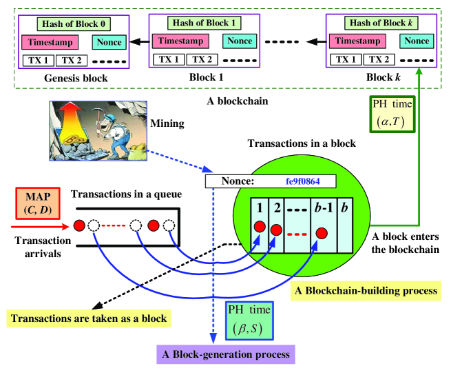
Figure 1: A blockchain queueing system under Markovian environment

From Figure 1, now we provide some model descriptions as follows:

Arrival process: Transactions arrive at the blockchain system according to a Markovian arrival process (MAP) with representation $\left(C,D\right)$ of order $m_{0}$, where the matrix $C+D$ is the infinitesimal generator of an irreducible Markov process; $C$ indicates the state transition rates that only the random environment changes without any transaction arrival, $D$ denotes the arrival rates of transactions under the random environment $C$; $\left(C+D\right)e=0$, and $e$ is a column vector of suitable size in which each element is one. Obviously, the Markov process $C+D$ with finite states is irreducible and positive recurrent. Let $\mathbf{\omega}$ be the stationary probability vector of the Markov process $C+D$, it is clear that $\omega\left(C+D\right)=0$ and $\omega e=1$. Also, the stationary arrival rate of the MAP is given by $\lambda=\omega De$.

In addition, we assume that each arriving transaction must first enter a queueing waiting room of infinite size. See the lower left part corner of Figure 1.

A block-generation process: Each arriving transaction first needs to queue in a waiting room. Then it is possibly chosen into a block of the maximal size $b$. This is regarded as the first stage of service, called block-generation process. Note that the arriving transactions will be continually chosen into the block until the block-generation process is over under which a nonce is appended to the block by a mining winner. See the lower middle part of Figure 1 for more details.

The block-generation time begins the initial epoch of a mining process until a nonce of the block is found (i.e., the cryptographic mathematical puzzle is solved for sending a nonce to the block), then the mining process is terminated immediately. We assume that all the block-generation times are i.i.d., and are of phase type with an irreducible representation $\left(\beta,S\right)$ of order $m_{2}$, where $\beta e=1$, the expected blockchain-building time is given by $1/\mu_{2}=-\beta S^{-1}e$.

The block-generation discipline: A block can consist of some transactions but at most $b$ transactions. Once the mining process begins, the transactions are chosen into a block, in which they are not completely based on the First Come First Service (FCFS) from the order of transaction arrivals. In this case, several transactions in the back of this queue may also be preferentially chosen into the block. When the block is formed, it will not receive any new arriving transaction. See the lower middle part of Figure 1.

A blockchain-building process: Once the mining process is over, the block with a group of transactions will be pegged to a blockchain. This is regarded as the second stage of service due to the network latency, called blockchain-building process, see the lower right corner of Figure 1. In addition, the upper part of Figure 1 also outlines the blockchain and the internal structure of every block.

In the blockchain system, we assume that the blockchain-building times are i.i.d, and have a common PH-distribution with an irreducible representation $\left(\alpha,T\right)$ of order $m_{1}$, where $\alpha e=1$, and the expected block-generation time is given by $1/\mu_{1}=-\alpha T^{-1}e$.

The maximum block size: To avoid the spam attacks, the maximum size of each block is limited. We assume that there are at most $b$ transactions in each block. If there are more than $b$ transactions in the queueing waiting room, then the $b$ transactions are chosen into a full block so that those redundant transactions are left in the queueing waiting room in order to set up another possible block. In addition, the block size $b$ maximizes the batch service ability in the blockchain system.

Independence: We assume that all the random variables defined above are independent of each other.

Remark 1

This paper is the first one to consider a blockchain system with non-Poisson transaction arrivals (MAPs) and with non-exponential block-generation and blockchain-building times (PH distributions), and it also provides a detailed analysis for the blockchain queueing model by means of the block-structured Markov processes and the $RG$-factorizations. However, so far analysis of the blockchain queues with renewal arrival process or with general service time distributions has still been an interesting open problem in queueing research of blockchain systems.

Remark 2

In the blockchain system, there are some key factors including the maximum block size, mining reward, transaction fee, mining strategy, security of blockchain and so on. Based on this, we may develop reward queueing models, decision queueing models, and game queueing models in the study of blockchain systems. Therefore, analysis for the key factors will be not only theoretically necessary but also practically important in development of blockchain technologies.

3 A Markov Process of GI/M/1 Type

In this section, to analyze the blockchain queueing system, we first establish a continuous-time Markov process of GI/M/1 type. Then we derive a system stable condition and express the stationary probability vector of the blockchain queueing system by means of the matrix-geometric solution.

Let $N_{1}\left(t\right),N_{2}\left(t\right),I\left(t\right),J_{1}\left(t\right)$ and$\ J_{2}\left(t\right)$ be the number of transactions in the queueing waiting room, the number of transactions in the block, the phase of the MAP, the phase of a blockchain-building PH time, and the phase of a block-generation PH time at time $t$, respectively. We write $\mathbf{X}=\left\{\left(N_{1}\left(t\right),N_{2}\left(t\right),I\left(t\right),J_{1}\left(t\right),J_{2}\left(t\right)\right),t\geq 0\right\}$. Then it is easy to see that $\mathbf{X}$ is a continuous-time Markov process with block structure whose state space is given by

$$\mathbf{\Omega}= \left\{\left(0,0;i\right),1\leq i\leq m_{0}\right\}$$

$$\cup\left\{\left(0,l;i,j\right),1\leq l\leq b,1\leq i\leq m_{0},1\leq j\leq m_{1}\right\}$$

$$\cup\left\{\left(k,0;i,r\right),k\geq 1,1\leq i\leq m_{0},1\leq r\leq m_{2}\right\}$$

$$\cup\left\{\left(k,l;i,j\right),k\geq 1,1\leq l\leq b,1\leq i\leq m_{0},1\leq j\leq m_{1}\right\}.$$

From Figure 1, it is easy to set up the state transition relation of the Markov process $\mathbf{X}$, see Figure 2 for more details. It is a key in understanding of Figure 2 that there is a different transition between State $\left(k,0\right)$ for the block-generation and State $\left(k,l\right)$ for the blockchain-building with $1\leq l\leq b$ because the block-generation and blockchain-building processes can not simultaneously exist at a time, and specifically, a block must first be generated, then it can enter the blockchain-building process.

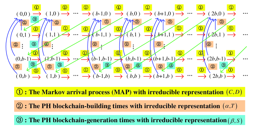
Figure 2: State transition relation of the Markov process

By using Figure 2, the infinitesimal generator of the Markov process $\mathbf{X}$ is given by

$$\mathbf{Q}=\left(\begin{array}[c]{ccccccccc}B_{1}&B_{0}&&&&&&&\\ B_{2}&A_{1}&A_{0}&&&&&&\\ B_{3}&&A_{1}&A_{0}&&&&&\\ \vdots&&&\ddots&\ddots&&&&\\ B_{b+1}&&&&A_{1}&A_{0}&&&\\ &A_{b+1}&&&&A_{1}&A_{0}&&\\ &&A_{b+1}&&&&A_{1}&A_{0}&\\ &&&\ddots&&&&\ddots&\ddots\end{array}\right),$$ (1)

where $\otimes$ and $\oplus$ are the Kronecker product and the Kronecker sum of two matrices, respectively,

$$A_{0}=\left(\begin{array}[c]{cccc}D\otimes I&&&\\ &D\otimes I&&\\ &&\ddots&\\ &&&D\otimes I\end{array}\right),\text{ }A_{1}=\left(\begin{array}[c]{cccc}C\oplus S&&&\\ I\otimes\left(T^{0}\beta\right)&C\oplus T&&\\ \vdots&&\ddots&\\ I\otimes\left(T^{0}\beta\right)&&&C\oplus T\end{array}\right),$$

$$A_{b+1}=\left(\begin{array}[c]{cccc}0&\cdots&0&I\otimes\left(S^{0}\alpha\right)\\ &&&\\ &&&\\ &&&\end{array}\right),$$

and

$$B_{0}=\left(\begin{array}[c]{cccc}D\otimes\beta&&&\\ &D\otimes I&&\\ &&\ddots&\\ &&&D\otimes I\end{array}\right),\text{ }B_{1}=\left(\begin{array}[c]{cccc}C&&&\\ I\otimes T^{0}&C\oplus T&&\\ \vdots&&\ddots&\\ I\otimes T^{0}&&&C\oplus T\end{array}\right),$$

$$B_{2}=\left(\begin{array}[c]{ccccc}0&I\otimes\left(S^{0}\alpha\right)&0&\cdots&0\\ &&&&\\ &&&&\\ &&&&\end{array}\right),\text{ \ }\ldots,\text{ \ }B_{b+1}=\left(\begin{array}[c]{cccc}0&\cdots&0&I\otimes\left(S^{0}\alpha\right)\\ &&&\\ &&&\\ &&&\end{array}\right).$$

Clearly, the continuous-time Markov process $\mathbf{X}$ is of GI/M/1 type.

Now, we use the mean drift method to discuss the system stable condition of the continuous-time Markov process $\mathbf{X}$ of GI/M/1 type. Note that the mean drift method for checking system stability is given a detailed introduction in Chapter 3 of Li [54].

From Chapter 1 of Neuts [67] or Chapter 3 of Li [54], for the Markov process of GI/M/1 type, we write

$$\mathbf{A} =A_{0}+A_{1}+A_{b+1}$$

$$=\left(\begin{array}[c]{ccccc}D\otimes I+C\oplus S&&&&I\otimes\left(S^{0}\alpha\right)\\ I\otimes\left(T^{0}\beta\right)&D\otimes I+C\oplus T&&&\\ \vdots&&\ddots&&\\ I\otimes\left(T^{0}\beta\right)&&&D\otimes I+C\oplus T&\\ I\otimes\left(T^{0}\beta\right)&&&&D\otimes I+C\oplus T\end{array}\right).$$

Clearly, the matrix $\mathbf{A}$ is the infinitesimal generator of an irreducible, aperiodic and positive recurrent Markov process with two levels (i.e., Levels $0$ and $b$), together with $b-1$ instantaneous levels (i.e., Levels $1,2,...,b-1$) which will vanish as the time $t$ goes to infinity. On the other hand, such a special Markov process $\mathbf{A}$ will not influence applications of the matrix-geometric solution because it is only related to the mean drift method for establishing system stable conditions.

The following theorem discusses the invariant measure $\theta$ of the Markov process $\mathbf{A}$, that is, the vector $\theta$ satisfies the system of linear equations $\theta\mathbf{A}=0$ and $\theta e=1$.

Theorem 1

There exists the unique invariant measure $\theta=\left(\theta_{0},0,\ldots,0,\theta_{b}\right)$ of the Markov process $\mathbf{A}$, where $\left(\theta_{0},\theta_{b}\right)$ is the stationary probability vector of the irreducible positive-recurrent Markov process whose infinitesimal generator

$$\Re=\left(\begin{array}[c]{cc}D\otimes I+C\oplus S&I\otimes\left(S^{0}\alpha\right)\\ I\otimes\left(T^{0}\beta\right)&D\otimes I+C\oplus T\end{array}\right).$$

Proof: It follows from $\theta\mathbf{A}=0$ that

$$\theta_{1}\left(D\otimes I+C\oplus S\right)+\sum_{k=1}^{b-1}\theta_{k}\left[I\otimes\left(T^{0}\beta\right)\right]+\theta_{b}\left[I\otimes\left(T^{0}\beta\right)\right]=0\mathbf{,}$$ (2)

$$\theta_{k}\left[D\otimes I+C\oplus T\right]=0,\text{ \ }1\leq k\leq b-1,$$ (3)

$$\theta_{1}\left[I\otimes\left(S^{0}\alpha\right)\right]+\theta_{b}\left(D\otimes I+C\oplus T\right)=0.$$ (4)

For Equation (3), note that

$$D\otimes I+C\oplus T =D\otimes I+C\otimes I+I\otimes T$$

$$=\left(C+D\right)\otimes I+I\otimes T$$

$$=\left(C+D\right)\oplus T,$$

where $C+D$ is the infinitesimal generator of an irreducible and a positive-recurrent Markov process, thus its eigenvalue of the maximal real part is zero so that all the other eigenvalues have a negative real part; while $T$, coming from the PH distribution with irreducible representation $\left(\alpha,T\right)$, is invertible with the real part of each eigenvalue be negative due to the fact that $Te\lvertneqq 0$, and the matrix $T$ has the properties that all diagonal elements are negative, and all off-diagonal elements are nonnegative. Note that each eigenvalue of the matrix $\left(C+D\right)\oplus T$ are the sum of an eigenvalue of the matrix $C+D$ and an eigenvalue of the matrix $T$, thus each eigenvalue of the matrix $\left(C+D\right)\oplus T$ has a negative real part (i.e., it is non-zero). This shows that the matrix $\left(C+D\right)\oplus T$ is invertible by means of det$\left(\left(C+D\right)\oplus T\right)\neq 0$, which is the product of all the eigenvalues of $\left(C+D\right)\oplus T$. Hence, from Equation $\theta_{k}\left[D\otimes I+C\oplus T\right]=0$ for $1\leq k\leq b-1$, we obtain

$$\theta_{1}=\theta_{2}=\cdots=\theta_{b-1}=0.$$

This gives

$$\theta=\left(\theta_{0},0,\ldots,0,\theta_{b}\right).$$

It follows from (2) and (4) that

$$\left\{\begin{array}[c]{c}\theta_{0}\left(D\otimes I+C\oplus S\right)+\theta_{b}\left[I\otimes\left(T^{0}\beta\right)\right]=0\mathbf{,}\\ \theta_{0}\left[I\otimes\left(S^{0}\alpha\right)\right]+\theta_{b}\left(D\otimes I+C\oplus T\right)=0\mathbf{.}\end{array}\right.$$

Thus we have

$$\left(\theta_{0},\theta_{b}\right)\left(\begin{array}[c]{cc}D\otimes I+C\oplus S&I\otimes\left(S^{0}\alpha\right)\\ I\otimes\left(T^{0}\beta\right)&D\otimes I+C\oplus T\end{array}\right)=\left(0,0\right).$$

Let

$$\Re=\left(\begin{array}[c]{cc}D\otimes I+C\oplus S&I\otimes\left(S^{0}\alpha\right)\\ I\otimes\left(T^{0}\beta\right)&D\otimes I+C\oplus T\end{array}\right).$$

Then the matrix $\Re$ is the infinitesimal generator of an irreducible positive-recurrent Markov process. Thus the Markov process $\Re$ exists the stationary probability vector $\left(\theta_{0},\theta_{b}\right)$, that is, there exists the unique solution to the system of linear equations: $\left(\theta_{0},\theta_{b}\right)\Re=0$ and $\theta_{0}e+\theta_{b}e=1$. This completes the proof.  

The following theorem provides a necessary and sufficient conditions under which the Markov process $\mathbf{Q}$ is positive recurrence.

Theorem 2

The Markv process $\mathbf{Q}$ of GI/M/1 type is positive recurrent if and only if

$$\left(\theta_{0}+\theta_{b}\right)\left(D\otimes I\right)e<b\theta_{0}\left[I\otimes\left(S^{0}\alpha\right)\right]e.$$ (5)

Proof: By using the mean drift method given in Chapter 3 of Li [18] (e.g., Theorem 3.19 and the continuous-time case in Page 172), it is easy to see that the Markv process $\mathbf{Q}$ of GI/M/1 type is positive recurrent if and only if

$$\theta A_{0}e<b\theta A_{b+1}e.$$ (6)

Note that

$$\theta A_{0}e =\theta_{0}\left(D\otimes I\right)e+\theta_{b}\left(D\otimes I\right)e$$

$$=\left(\theta_{0}+\theta_{b}\right)\left(D\otimes I\right)e$$ (7)

and

$$b\theta A_{b+1}e=b\theta_{0}\left[I\otimes\left(S^{0}\alpha\right)\right]e,$$ (8)

thus we obtain

$$\left(\theta_{0}+\theta_{b}\right)\left(D\otimes I\right)e<b\theta_{0}\left[I\otimes\left(S^{0}\alpha\right)\right]e.$$

This completes the proof.  

It is necessary to consider a special case in which the transaction inputs are Poisson with arrival rate $\lambda$, and the blockchain-building and block-generation times are exponential with service rates $\mu_{1}$ and $\mu_{2}$, respectively. Note that this special case was studied in Li et al. [56], here we only restate the stable condition as the following corollary.

Corollary 3

The Markov process $\mathbf{Q}$ of GI/M/1 type is positive recurrent if and only if

$$\frac{b\mu_{1}\mu_{2}}{\mu_{1}+\mu_{2}}>\lambda.$$ (9)

By observing (9), it is easy to see that $1/\left(b\mu_{1}\right)+$ $1/\left(b\mu_{2}\right)<1/\lambda$, that is, the complicated service speed of transactions is faster than the transaction arrival speed, under which the Markov process $\mathbf{Q}$ of GI/M/1 type is positive recurrent. However, it is not easy to understood from (5).

If the Markv process $\mathbf{Q}$ of GI/M/1 type is positive recurrent, we write its stationary probability vector as

$$\mathbf{\pi}=\left(\mathbf{\pi}_{0},\mathbf{\pi}_{1},\mathbf{\pi}_{2},\ldots\right),$$

where for $k=0$

$$\mathbf{\pi}_{0}=\left(\pi_{0,0},\pi_{0,1},\ldots,\pi_{0,b}\right),$$

$$\pi_{0,0}=\left(\pi_{0,0}^{\left(i\right)}:1\leq i\leq m_{0}\right),$$

and for $1\leq l\leq b$

$$\pi_{0,l}=\left(\pi_{0,l}^{\left(i,j\right)}:1\leq i\leq m_{0},1\leq j\leq m_{1}\right);$$

for $k\geq 1$

$$\mathbf{\pi}_{k}=\left(\pi_{k,0},\pi_{k,1},\ldots,\pi_{k,b}\right),$$

$$\pi_{k,0}=\left(\pi_{k,0}^{\left(i,r\right)}:1\leq i\leq m_{0},1\leq r\leq m_{2}\right),$$

and for $1\leq l\leq b$

$$\pi_{k,l}=\left(\pi_{k,l}^{\left(i,j\right)}:1\leq i\leq m_{0},1\leq j\leq m_{1}\right).$$

Note that in the above expressions, the vector $\mathbf{a}=\left(a^{\left(i,j\right)}:1\leq i\leq I,1\leq j\leq J\right)$ is based on the lexicographical order of the elements, that is,

$$\mathbf{a}=\left(a^{\left(1,1\right)},a^{\left(1,2\right)},\ldots,a^{\left(1,J\right)};a^{\left(2,1\right)},a^{\left(2,2\right)},\ldots,a^{\left(2,J\right)};\ldots;a^{\left(I,1\right)},a^{\left(I,2\right)},\ldots,a^{\left(I,J\right)}\right).$$

If $\left(\theta_{0}+\theta_{b}\right)\left(D\otimes I\right)e<b\theta_{0}\left[I\otimes\left(S^{0}\alpha\right)\right]e$, then the Markv process $\mathbf{Q}$ of GI/M/1 type is irreducible and positive recurrent. Thus the Markov process $\mathbf{Q}$ exists a unique stationary probability vector, which is also matrix-geometric. Thus, to express the matrix-geometric stationary probability vector, we need to first obtain the rate matrix $R$, which is the minimal nonnegative solution to the following nonlinear matrix equation

$$R^{b+1}A_{b+1}+RA_{1}+A_{0}=0.$$ (10)

In general, it is very complicated to solve this nonlinear matrix equation (10) due to the term $R^{b+1}A_{b+1}$ of size $b+1$. In fact, for the blockchain queueing system, here we can not provide an explicit expression for the rate matrix $R$ yet. In this case, we can use some iterative algorithms, given in Neuts [67], to give its numerical solution. For example, an effective iterative algorithm given in Neuts [67] is described as

$$R_{0} =0\mathbf{,}$$

$$R_{N+1} =\left(R_{N}^{b+1}A_{b+1}+A_{0}\right)\left(-A_{1}\right)^{-1}.$$

Note that this algorithm is fast convergent, that is, after a finite number of iterative steps, we can numerically obtain a solution of higher precision which is used to approximate the rate matrix $R$.

The following theorem directly comes from Theorem 1.2.1 of Chapter 1 in Neuts [67]. Here, we restate it without a proof.

Theorem 4

If the Markv process $\mathbf{Q}$ of GI/M/1 type is positive recurrent, then the stationary probability vector $\mathbf{\pi}=\left(\mathbf{\pi}_{0},\mathbf{\pi}_{1},\mathbf{\pi}_{2},\ldots\right)$ is given by

$$\mathbf{\pi}_{k}=\mathbf{\pi}_{1}R^{k-1},\ \ \ k\geq 2.$$ (11)

where the vector $\left(\mathbf{\pi}_{0},\mathbf{\pi}_{1}\right)$ is the stationary probability vector of the censoring Markov process $\mathbf{Q}^{\left(1,2\right)}$ of levels $0$ and $1$ which is irreducible and positive recurrent. Thus it is the unique solution to the following system of linear equations:

$$\left\{\begin{array}[c]{c}\left(\mathbf{\pi}_{0},\mathbf{\pi}_{1}\right)\mathbf{Q}^{\left(1,2\right)}=\left(\mathbf{\pi}_{0},\mathbf{\pi}_{1}\right),\\ \mathbf{\pi}_{0}e+\mathbf{\pi}_{1}\left(I-R\right)^{-1}e=1,\end{array}\right.$$ (12)

where

$$\mathbf{Q}^{\left(1,2\right)}=\left(\begin{array}[c]{cc}B_{1}&B_{0}\\ \sum\limits_{k=2}^{b+1}R^{k-2}B_{k}&A_{1}+R^{b}A_{b+1}\end{array}\right).$$

Proof: Here, we only derive the boundary condition (12). It follows from $\mathbf{\pi Q}=0$ that

$$\left\{\begin{array}[c]{l}\pi_{0}B_{1}+\pi_{1}B_{2}+\cdots+\pi_{b}B_{b+1}=0,\\ \pi_{0}B_{0}+\pi_{1}A_{1}+\pi_{b+1}A_{b+1}=0.\end{array}\right.$$

By using the matrix-geometric solution $\mathbf{\pi}_{k}=\mathbf{\pi}_{1}R^{k-1}$ for $k\geq 2$, we have

$$\left\{\begin{array}[c]{l}\pi_{0}B_{1}+\pi_{1}\left(B_{2}+RB_{3}+\cdots+R^{b-1}B_{b+1}\right)=0,\\ \pi_{0}B_{0}+\pi_{1}\left(A_{1}+R^{b}A_{b+1}\right)=0.\end{array}\right.$$

This gives the desired result, and completes the proof.  

4 The Stationary Transaction Numbers

In this section, we discuss two key performance measures: The average stationary numbers of transactions both in the queueing waiting room and in the block, and give their simple expressions by means of the vectors $\mathbf{\pi}_{0}$ and $\mathbf{\pi}_{1}$, and the rate matrix $R$. Finally, we use numerical examples to verify computability of our theoretical results, and show how the performance measures depend on the main parameters of this system.

If $\left(\theta_{0}+\theta_{b}\right)\left(D\otimes I\right)e<b\theta_{0}\left[I\otimes\left(S^{0}\alpha\right)\right]e$, then the blockchain system is stable. In this case, we write that w.p.1,

$$N_{1}=lim_{t\rightarrow+\infty}N_{1}\left(t\right),\ \ \ N_{2}=lim_{t\rightarrow+\infty}N_{2}\left(t\right),$$

where $N_{1}\left(t\right)$ and $N_{2}\left(t\right)$ are the numbers of transactions in the queueing waiting room and of transactions in the block at time $t\geq 0$, respectively.

(a) The average stationary number of transactions in the queueing waiting room

It follows from (11) and (12) that

$$E\left[N_{1}\right] =\overset{\infty}{\underset{k=1}{\sum}}k\overset{m_{0}}{\underset{i=1}{\sum}}\overset{m_{2}}{\underset{r=1}{\sum}}\pi_{k,0}^{\left(i,r\right)}+\overset{\infty}{\underset{k=1}{\sum}}k\underset{l=1}{\overset{b}{\sum}}\overset{m_{0}}{\underset{i=1}{\sum}}\overset{m_{1}}{\underset{j=1}{\sum}}\pi_{k,l}^{\left(i,j\right)}$$

$$=\overset{\infty}{\underset{k=1}{\sum}}k\underset{l=0}{\overset{b}{\sum}}\mathbf{\pi}_{k,l}\text{ }e$$

$$=\overset{\infty}{\underset{k=1}{\sum}}k\text{ }\mathbf{\pi}_{k}\text{ }e=\mathbf{\pi}_{1}R\left(I-R\right)^{-2}e.$$

Note that the above three vectors $e$ has different sizes, for example, the size of the first one is $m_{0}\times m_{2}$ for $l=0$ and $m_{0}\times m_{1}$ for $1\leq l\leq b$; while the sizes of the second and third are $m_{0}\times\left(m_{2}+bm_{1}\right)$. For simplicity of description, here we use only a vector $e$ whose size can easily be inferred by the context.

(b) The average stationary number of transactions in the block

Let $\mathbf{h}=\left(0,e,2e,\ldots,be\right)^{T}$. Then

$$E\left[N_{2}\right] =\underset{l=0}{\overset{b}{\sum}}l\overset{\infty}{\underset{k=0}{\sum}}\overset{m_{0}}{\underset{i=1}{\sum}}\overset{m_{1}}{\underset{j=1}{\sum}}\pi_{k,l}^{\left(i,j\right)}$$

$$=\underset{l=0}{\overset{b}{\sum}}l\overset{\infty}{\underset{k=0}{\sum}}\mathbf{\pi}_{k,l}\text{ }e$$

$$=\overset{\infty}{\underset{k=0}{\sum}}\mathbf{\pi}_{k}\text{ }\mathbf{h}$$

$$=\left[\mathbf{\mathbf{\pi}_{0}+\pi}_{1}\left(I-R\right)^{-1}\right]\text{ }\mathbf{h}.$$

In the remainder of this section, we provide some numerical examples to verify computability of our theoretical results, and to analyze how the two performance measures $E\left[N_{1}\right]$ and $E\left[N_{2}\right]$ depend on some crucial parameters of the blockchain queueing system.

In the two numerical examples, we take some common parameters: The block-building service rate $\mu_{1}\in\left[0.05,1.5\right]$, the block-generation service rate $\mu_{2}=2$, the arrival rate $\lambda=0.3$, the maximum block size $b=40,320,1000$, respectively.

From Figure 3, it is seen that $E\left[N_{1}\right]$ and $E\left[N_{2}\right]$ decrease, as $\mu_{1}$ increases. At the same time, $E\left[N_{1}\right]$ decreases as $b$ increases, but $E\left[N_{2}\right]$ increases as $b$ increases.

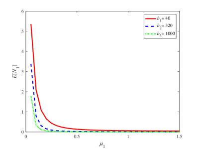
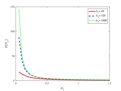
Figure 3: $E\left[N_{1}\right]$, $E\left[N_{2}\right]$ vs. $\mu_{1}$ under three different values of $b$

5 The Transaction-Confirmation Time

In this section, we provide a matrix-analytic method based on the $RG$-factorizations for computing the average transaction-confirmation time of any transaction, which is always an interesting but difficult topic because of the batch service for a block of transactions, and the Service-In-Random-Order for choosing some transactions into a block.

In the blockchain system, the transaction-confirmation time is the time interval from the time epoch that a transaction arrives at the queueing waiting room to the time point that the block including the transaction is first confirmed and then it is built in the blockchain. Obviously, the transaction-confirmation time is the sojourn time of the transaction in the blockchain system, and it is the sum of the block-generation and blockchain-building times of a transaction taken in the block. Let $\Im$ denote the transaction-confirmation time of any transaction when the blockchain system is stable.

To study the transaction-confirmation time $\Im$, we need to introduce the stationary life time $\Gamma_{s}$ of the PH blockchain-building time $\Gamma$ with an irreducible representation $\left(\alpha,T\right)$. Let $\varpi$ be the stationary probability vector of the Markov process $T+T^{0}\alpha$. Then the stationary life time $\Gamma_{s}$ is also a PH distribution with an irreducible representation $\left(\varpi,T\right)$, e.g., see Property 1.5 in Chapter 1 of Li [54]. Clearly, $E\left[\Gamma_{s}\right]=-\varpi T^{-1}e.$

Now, we introduce a Markov process $\left\{Y\left(t\right):t\geq 0\right\}$ with an absorbing state, whose state transition relation given in Figure 4 according to Figures 1 and 2. At the same time, we define the first passage time as

$$\xi=\inf\left\{t:Y\left(t\right)=\text{the absorbing state, }t\geq 0\right\}.$$

For $k\geq 0,1\leq i\leq m_{0}$ and $1\leq r\leq m_{2}$, if $Y\left(0\right)=$ $\left(k,0;i,r\right)$, then we write the first passage time as $\xi_{|\left(k,0;i,r\right)}$.

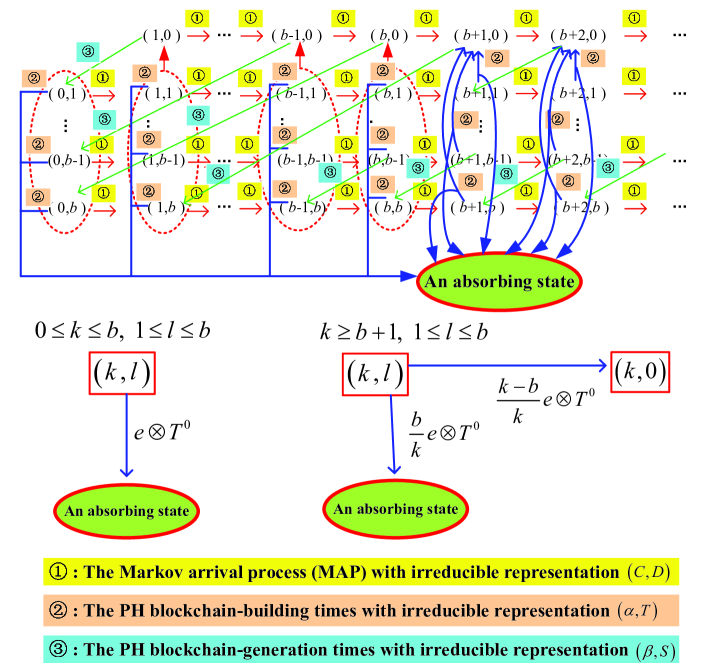
Figure 4: State transition relation of the Markov process with an absorbing state

Remark 3

It is necessary to explain the absorbing rates in the below part of Figure 4.

(1) If $Y\left(0\right)=\left(k,l\right)$ for $1\leq k\leq b$ and $0\leq l\leq b$, then the $k$ transactions can be chosen into a block once the previous block is pegged to the blockchain, a tagged transaction of the $k$ transactions is chosen into the block with probability $1$.

(2) If $Y\left(0\right)=\left(k,l\right)$ for $k\geq b+1$ and $0\leq l\leq b$, then any $b$ transactions of the $k$ transactions can randomly be chosen into a block once the previous block is pegged to the blockchain, thus a tagged transaction of the $k$ transactions is chosen into the block of the maximal size $b$ with probability $b/k$.

When a transaction arrives at the queueing waiting room, it can observes the states of the blockchain system having two different cases:

Case one: State $\left(k,0;i,r\right)$ for $k\geq 1;1\leq i\leq m_{0}$ and $1\leq r\leq m_{2}$. In this case, with the initial probability $\pi_{k,0}^{\left(i,r\right)}$, the transaction-confirmation time $\Im$ is the first passage time $\xi_{|\left(k,0;i,r\right)}$ of the Markov process with an absorbing state, whose state transition relation given in Figure 4.

Case two: State $\left(k,l;i,r\right)$ for $k\geq 1,1\leq l\leq b;1\leq i\leq m_{0}$ and $1\leq j\leq m_{1}$. In this case, with the initial probability $\pi_{k,l}^{\left(i,j\right)}$, the transaction-confirmation time $\Im$ is decomposed into the sum of the random variable $\Gamma_{s}$ and the first passage time $\xi_{|\left(k,0;i,r\right)}$ given in Case one. It is easy to see Figure 4 that there exists a stochastic decomposition: $\Im=\Gamma_{s}+\xi_{|\left(k,0;i,r\right)}$.

For the above analysis, it is easy to see that computation of the first passage time $\xi_{|\left(k,0;i,r\right)}$ is a key in analyzing the transaction-confirmation time.

Based on the state transition relation given in Figure 4, now we write the infinitesimal generator of the Markov process $\left\{Y\left(t\right):t\geq 0\right\}$ as

$$\mathbf{H}=\left(\begin{array}[c]{ccccccccc}\widetilde{B}_{1}&\widetilde{B}_{0}&&&&&&&\\ \widetilde{B}_{2}&\widetilde{A}_{1}&A_{0}&&&&&&\\ \widetilde{B}_{3}&&\widetilde{A}_{1}&A_{0}&&&&&\\ \vdots&&&\ddots&\ddots&&&&\\ \widetilde{B}_{b+1}&&&&\widetilde{A}_{1}&A_{0}&&&\\ &A_{b+1}&&&&\widetilde{A}_{1}^{\left(b+1\right)}&A_{0}&&\\ &&A_{b+1}&&&&\widetilde{A}_{1}^{\left(b+2\right)}&A_{0}&\\ &&&\ddots&&&&\ddots&\ddots\end{array}\right),$$ (13)

where

$$A_{0}=\left(\begin{array}[c]{cccc}D\otimes I&&&\\ &D\otimes I&&\\ &&\ddots&\\ &&&D\otimes I\end{array}\right),\text{ }A_{b+1}=\left(\begin{array}[c]{cccc}0&\cdots&0&I\otimes\left(S^{0}\alpha\right)\\ &&&\\ &&&\\ &&&\end{array}\right),$$

$$\widetilde{A}_{1}=\left(\begin{array}[c]{cccc}C\oplus S&&&\\ &C\oplus T&&\\ &&\ddots&\\ &&&C\oplus T\end{array}\right),$$

for $k\geq b+1$

$$\widetilde{A}_{1}^{\left(k\right)}=\left(\begin{array}[c]{cccc}C\oplus S&&&\\ I\otimes\left(\frac{k-b}{k}T^{0}\beta\right)&C\oplus T&&\\ \vdots&&\ddots&\\ I\otimes\left(\frac{k-b}{k}T^{0}\beta\right)&&&C\oplus T\end{array}\right);$$

$$\widetilde{B}_{0}=\left(\begin{array}[c]{ccccc}0&D\otimes I&&&\\ &&D\otimes I&&\\ &&&\ddots&\\ &&&&D\otimes I\end{array}\right),\text{ }\widetilde{B}_{1}=\left(\begin{array}[c]{cccc}C\otimes I&&&\\ &C\oplus T&&\\ &&\ddots&\\ &&&C\oplus T\end{array}\right),$$

$$\widetilde{B}_{2}=\left(\begin{array}[c]{ccccc}I\otimes\left(S^{0}\alpha\right)&0&0&\cdots&0\\ &&&&\\ &&&&\\ &&&&\end{array}\right),\text{ \ }\ldots,\text{ \ }\widetilde{B}_{b+1}=\left(\begin{array}[c]{cccc}0&\cdots&0&I\otimes\left(S^{0}\alpha\right)\\ &&&\\ &&&\\ &&&\end{array}\right).$$

If the blockchain system is stable, then the probability that a transaction observes State $\left(0,0;i\right)$ only after arrived at the instant is $\pi_{1,0}^{\left(i,r\right)}$; for $1\leq l\leq b$, the probability that a transaction observes State $\left(0,l;i,j\right)$ only after arrived at the instant is $\pi_{1,l}^{\left(i,j\right)}$; for $k\geq 2$, the probability that a transaction observes State $\left(k-1,0;i,r\right)$ only after arrived at the instant is $\pi_{k,0}^{\left(i,r\right)}$; for $k\geq 2,1\leq l\leq b$, the probability that a transaction observes State $\left(k-1,l;i,j\right)$ only after arrived at the instant is $\pi_{k,l}^{\left(i,j\right)}$. Obviously, for $0\leq l\leq b$, States $\left(0,0;i\right)$ and $\left(0,l;i,j\right)$ will not be encountered by the transaction only after arrived at the instant, thus the stationary probabilities $\pi_{0,0}^{\left(i\right)}$ and $\pi_{0,l}^{\left(i,j\right)}$ should be omitted by the observation of any arriving transaction. Based on this, we introduce a new initial probability vector for the observation of any transaction only after arrived at the instant as follows:

$$\mathbf{\gamma}=\left(\mathbf{\gamma}_{1},\mathbf{\gamma}_{2},\mathbf{\gamma}_{3},\ldots\right),$$

where for $k\geq 1$

$$\mathbf{\gamma}_{k}=\left(\gamma_{k,0},\gamma_{k,1},\ldots,\gamma_{k,b}\right),$$

$$\gamma_{k,0}=\left(\frac{1}{1-\mathbf{\pi}_{0}e}\pi_{k,0}^{\left(i,r\right)}:1\leq i\leq m_{0},1\leq r\leq m_{2}\right)$$

and for $1\leq l\leq b$

$$\gamma_{k,l}=\left(\frac{1}{1-\mathbf{\pi}_{0}e}\pi_{k,l}^{\left(i,j\right)}:1\leq i\leq m_{0},1\leq j\leq m_{1}\right).$$

To emphasize on the event that the transaction observes State $\left(k-1,0;i,r\right)$ only after arrived at the instant, we introduce a new initial probability vector

$$\mathbf{\varphi}=\left(\mathbf{\varphi}_{1},\mathbf{\varphi}_{2},\mathbf{\varphi}_{3},\ldots\right),$$

where for $k\geq 1$

$$\mathbf{\varphi}_{k}=\left(\gamma_{k,0},0,0,\ldots,0\right).$$

In addition, we take

$$\mathbf{\psi}=\mathbf{\gamma-\varphi.}$$

Theorem 5

If the blockchain system is stable, then the first passage time $\xi_{|\left(k,0;i,r\right)}$ is a PH distribution of infinite size with an irreducible representation $\left(\eta\left(k,0;i,r\right),\mathbf{H}\right)$, where $\mathbf{H}$ is given in (13), and

$$\eta\left(k,0;i,r\right)=\left(0,0,\ldots,0,\frac{1}{1-\mathbf{\pi}_{0}e}\pi_{k,0}^{\left(i,r\right)},0,0,\ldots,0\right).$$

Also, we have

$$\mathbf{H}^{0} =-\mathbf{H}e$$

$$=\left(e\otimes T^{0},e\otimes T^{0},\ldots,e\otimes T^{0};\frac{b}{b+1}e\otimes T^{0},\frac{b}{b+2}e\otimes T^{0},\ldots\right).$$

Proof: If the blockchain system is stable, then $\xi_{|\left(k,0;i,r\right)}$ is the first passage time of the Markov process $\mathbf{H}$ (or $\left\{Y\left(t\right):t\geq 0\right\}$) with an absorbing state and under the initial state $Y\left(0\right)=$ $\left(k,0;i,r\right)$. Note that the original Markov process $\mathbf{Q}$ given in (1) is irreducible and positive recurrent, thus $\xi_{|\left(k,0;i,r\right)}$ is a PH distribution of infinite size with an irreducible representation $\left(\eta\left(k,0;i,r\right),\mathbf{H}\right)$. At the same time, a simple computation gives

$$\mathbf{H}^{0}=\left(e\otimes T^{0},e\otimes T^{0},\ldots,e\otimes T^{0};\frac{b}{b+1}e\otimes T^{0},\frac{b}{b+2}e\otimes T^{0},\ldots\right).$$

This completes the proof.  

Based on Theorem 5, now we extend the first passage time $\xi_{|\left(k,0;i,r\right)}$ to $\xi_{|\left(\mathbf{0},\mathbf{\varphi}\right)}$, which is the first passage time of the Markov process $\mathbf{H}$ with an initial probability vector $\left(\mathbf{0},\mathbf{\varphi}\right)$. The following corollary shows that $\xi_{|\left(\mathbf{0},\mathbf{\varphi}\right)}$ is PH distribution of infinite size, while its proof is easy and is omitted here.

Corollary 6

If the blockchain system is stable, then the first passage time $\xi_{|\left(\mathbf{0},\mathbf{\varphi}\right)}$ is a PH distribution of infinite size with an irreducible representation $\left(\left(\mathbf{0},\mathbf{\varphi}\right),\mathbf{H}\right)$, and

$$E\left[\xi_{|\left(\mathbf{0},\mathbf{\varphi}\right)}\right]=-\left(\mathbf{0},\mathbf{\varphi}\right)\mathbf{H}^{-1}e,$$

$$Var\left[\xi_{|\left(\mathbf{0},\mathbf{\varphi}\right)}\right]=\left(\mathbf{0},\mathbf{\varphi}\right)\mathbf{H}^{-2}e-\left[\left(\mathbf{0},\mathbf{\varphi}\right)\mathbf{H}^{-1}e\right]^{2}.$$

The following theorem provides a simple expression for the average transaction-confirmation time $E[\Im]$ by means of Corollary 6.

Theorem 7

If the blockchain queueing system is stable, then the average transaction-confirmation time $E[\Im]$ is given by

$$E\left[\Im\right]=E\left[\xi_{|\left(\mathbf{0},\mathbf{\varphi}\right)}\right]+\left(1-\mathbf{\varphi}e\right)E\left[\Gamma_{s}\right],$$

where $\Gamma_{s}$ is the stationary life time of the PH blockchain-building time with an irreducible representation $\left(\alpha,T\right)$. Further, we have

$$E\left[\Im\right]=-\left(\mathbf{0},\mathbf{\varphi}\right)\mathbf{H}^{-1}e-\left(1-\mathbf{\varphi}e\right)\varpi T^{-1}e,$$

where $\varpi$ is the stationary probability vector of the Markov process $T+T^{0}\alpha$.

Proof: We first introduce two basic events

$$\Theta= \left\{\text{The transaction observes States }\left(0,0;i\right)\text{ and }\left(k,0;i,r\right)\right.\text{\ }$$

$$\text{ }\left.\text{for }1\leq i\leq m_{0},k\geq 1,1\leq r\leq m_{2}\right.\text{ }$$

$$\left.\text{only after arrived at the instant}\right\}$$

and

$$\Theta^{c}= \left\{\text{The transaction observes States }\left(k,l;i,j\right)\right.\text{\ }$$

$$\text{ }\left.\text{for }k\geq 1,1\leq l\leq b,1\leq i\leq m_{0},1\leq j\leq m_{1}\right.\text{ }$$

$$\left.\text{only after arrived at the instant}\right\}.$$

It is easy to see that $\Theta\cup\Theta^{c}=\Omega$. Thus the two events is complementary according to the fact that the transaction can observe all the states of the Markov process $\mathbf{Q}$ only after arrived at the instant. If the blockchain system is stable, then it is easy to compute the probabilities of the two events as follows:

$$P\left\{\Theta\right\}=\left(\mathbf{0},\mathbf{\varphi}\right)e=\mathbf{\varphi}e$$

and

$$P\left\{\Theta^{c}\right\}=1-P\left\{\Theta\right\}=1-\mathbf{\varphi}e.$$

By using the law of total probability, we obtain

$$E\left[\Im\right] =P\left\{\Theta\right\}E\left[\Im\text{ }|\text{ }\Theta\right]+P\left\{\Theta^{c}\right\}E\left[\Im\text{ }|\text{ }\Theta^{c}\right]$$

$$=\mathbf{\varphi}e\text{ }E\left[\xi_{|\left(\mathbf{0},\mathbf{\varphi}\right)}\right]+\left(1-\mathbf{\varphi}e\right)E\left[\Gamma_{s}+\xi_{|\left(\mathbf{0},\mathbf{\varphi}\right)}\right]$$

$$=E\left[\xi_{|\left(\mathbf{0},\mathbf{\varphi}\right)}\right]+\left(1-\mathbf{\varphi}e\right)E\left[\Gamma_{s}\right]$$

$$=-\left(\mathbf{0},\mathbf{\varphi}\right)\mathbf{H}^{-1}e-\left(1-\mathbf{\varphi}e\right)\varpi T^{-1}e.$$

The proof is completed.  

As shown in Theorem 7, it is a key in the study of PH distributions of infinite sizes whether or not we can compute the inverse matrix $\mathbf{H}^{-1}$ of infinite size. To this end, we need to use the $RG$-factorizations, given in Li [54], to provide such a computable path. In what follows we provide only a simple interpretation on the computation, while some detailed discussions will be left in our another paper in the future.

In fact, it is often very difficult and challenging to compute the inverse of a matrix of infinite size only except for the triangular matrices. Fortunately, by using the $RG$-factorizations, the infinitesimal generator $\mathbf{H}$ can be decomposed into a product of three matrices: Two block-triangular matrices and a block-diagonal matrix. Therefore, the $RG$-factorizations play a key role to generalizing the PH distributions from finite dimensions to infinite dimensions.

By using Subsection 2.2.3 in Chapter 2 of Li [54] (see Pages 88 to 89), now we provide the UL-type $RG$-factorization of the infinitesimal generator $\mathbf{H}$. It will be seen that the $RG$-factorization of $\mathbf{H}$ has a beautiful block structure, which is well related to the special block characteristics of $\mathbf{H}$ corresponding to the blockchain system. To this end, we need to define and compute the $R$-, $U$- and $G$-measures as follows.

The $R$-measure. Let $R_{k}$ for $k\geq 0$ be the minimal nonnegative solution to the system of nonlinear matrix equations:

$$R_{0} =\widetilde{B}_{0}+R_{0}\widetilde{A}_{1}+R_{0}R_{1}\cdots R_{b-1}R_{b}A_{b+1},$$

$$R_{1} =A_{0}+R_{1}\widetilde{A}_{1}+R_{1}R_{2}\cdots R_{b}R_{b+1}A_{b+1},$$

$$R_{2} =A_{0}+R_{2}\widetilde{A}_{1}+R_{2}R_{3}\cdots R_{b+1}R_{b+2}A_{b+1},$$

$$\vdots$$

$$R_{b-1} =A_{0}+R_{b-1}\widetilde{A}_{1}+R_{b-1}R_{b}\cdots R_{2b-2}R_{2b-1}A_{b+1},$$

and

$$R_{b} =A_{0}+R_{b}\widetilde{A}_{1}^{\left(b+1\right)}+R_{b}R_{b+1}\cdots R_{2b-1}R_{2b}A_{b+1},$$

$$R_{b+1} =A_{0}+R_{b+1}\widetilde{A}_{1}^{\left(b+2\right)}+R_{b+1}R_{b+2}\cdots R_{2b}R_{2b+1}A_{b+1},$$

$$R_{b+2} =A_{0}+R_{b+2}\widetilde{A}_{1}^{\left(b+3\right)}+R_{b+2}R_{b+3}\cdots R_{2b+1}R_{2b+2}A_{b+1},$$

$$\vdots$$

The $U$-measure. Based on the $R$-measure $R_{k}$ for $k\geq 0$, we have

$$U_{0} =\widetilde{B}_{1}+R_{0}\widetilde{B}_{2}+R_{0}R_{1}\widetilde{B}_{3}+\cdots+R_{0}R_{1}\cdots R_{b-2}R_{b-1}\widetilde{B}_{b+1},$$

$$U_{1} =\widetilde{A}_{1}+R_{1}R_{2}\cdots R_{b-1}R_{b}A_{b+1},$$

$$U_{2} =\widetilde{A}_{1}+R_{2}R_{3}\cdots R_{b}R_{b+1}A_{b+1},$$

$$\vdots$$

$$U_{b} =\widetilde{A}_{1}+R_{b}R_{b+1}\cdots R_{2b-2}R_{2b-1}A_{b+1},$$

and

$$U_{b+1} =\widetilde{A}_{1}^{\left(b+1\right)}+R_{b+1}R_{b+2}\cdots R_{2b-1}R_{2b}A_{b+1},$$

$$U_{b+2} =\widetilde{A}_{1}^{\left(b+2\right)}+R_{b+2}R_{b+3}\cdots R_{2b}R_{2b+1}A_{b+1},$$

$$U_{b+3} =\widetilde{A}_{1}^{\left(b+3\right)}+R_{b+3}R_{b+4}\cdots R_{2b+1}R_{2b+2}A_{b+1},$$

$$\vdots$$

The $G$-measure. Based on the $R$-measure $R_{k}$ for $k\geq 0$ and the $U$-measure $U_{k}$ for $k\geq 0$, we have

$$G_{1,0} =\left(-U_{1}\right)^{-1}\left(\widetilde{B}_{2}+R_{1}\widetilde{B}_{3}+R_{1}R_{2}\widetilde{B}_{4}+\cdots+R_{1}R_{2}\cdots R_{b-2}R_{b-1}\widetilde{B}_{b+1}\right),$$

$$G_{2,0} =\left(-U_{2}\right)^{-1}\left(\widetilde{B}_{3}+R_{2}\widetilde{B}_{4}+R_{2}R_{3}\widetilde{B}_{5}+\cdots+R_{2}R_{3}\cdots R_{b-2}R_{b-1}\widetilde{B}_{b+1}\right),$$

$$\vdots$$

$$G_{b-1,0} =\left(-U_{b-1}\right)^{-1}\left(\widetilde{B}_{b}+R_{b-1}\widetilde{B}_{b+1}\right),$$

$$G_{b,0} =\left(-U_{b}\right)^{-1}\widetilde{B}_{b+1},$$

$$G_{2,1} =\left(-U_{2}\right)^{-1}R_{2}R_{3}\cdots R_{b-1}R_{b}A_{b+1},$$

$$G_{3,1} =\left(-U_{3}\right)^{-1}R_{3}R_{4}\cdots R_{b-1}R_{b}A_{b+1},$$

$$\vdots$$

$$G_{b,1} =\left(-U_{b}\right)^{-1}R_{b}A_{b+1},$$

$$G_{b+1,1} =\left(-U_{b+1}\right)^{-1}A_{b+1},$$

and for $k\geq 3$

$$G_{k,k-1} =\left(-U_{k}\right)^{-1}R_{k}R_{k+1}\cdots R_{k+b-3}R_{k+b-2}A_{b+1},$$

$$G_{k+1,k-1} =\left(-U_{k+1}\right)^{-1}R_{k+1}R_{k+2}\cdots R_{k+b-3}R_{k+b-2}A_{b+1},$$

$$\vdots$$

$$G_{k+b-2,k-1} =\left(-U_{k+b-2}\right)^{-1}R_{k+b-2}A_{b+1},$$

$$G_{k+b-1,k-1} =\left(-U_{k+b-1}\right)^{-1}A_{b+1}.$$

Based on the $R$-, $U$- and $G$-measures, we provide the UL-type $RG$-factorization of the infinitesimal generator $\mathbf{H}$ as follows:

$$\mathbf{H=}\left(I-\mathbf{R}_{U}\right)\mathbf{U}\left(I-\mathbf{G}_{L}\right),$$

where

$$\mathbf{R}_{U}=\left(\begin{array}[c]{cccccc}0&R_{0}&&&&\\ &0&R_{1}&&&\\ &&0&R_{2}&&\\ &&&0&R_{3}&\\ &&&&\ddots&\ddots\end{array}\right),$$

$$\mathbf{U}=\text{diag}\left(U_{0},U_{1},U_{2},U_{3},\ldots\right)$$

and

$$\mathbf{G}_{L}=\left(\begin{array}[c]{ccccccccc}0&&&&&&&&\\ G_{1,0}&0&&&&&&&\\ G_{2,0}&G_{2,1}&0&&&&&&\\ \vdots&\vdots&\vdots&\ddots&&&&&\\ G_{b-1,0}&G_{b-1,1}&G_{b-1,b-2}&\cdots&0&&&&\\ G_{b,0}&G_{b,1}&G_{b,b-2}&\cdots&G_{b,k}&0&&&\\ &G_{b+1,1}&G_{b+1,b-2}&\cdots&G_{b+1,k}&G_{b+1,k+1}&0&&\\ &&G_{b+2,b-2}&\cdots&G_{b+2,k}&G_{b+2,k+1}&G_{b+2,k+2}&0&\\ &&&\ddots&\vdots&\vdots&\vdots&\vdots&\ddots\end{array}\right).$$

Based on the UL-type $RG$-factorization $\mathbf{H=}\left(I-\mathbf{R}_{U}\right)\mathbf{U}\left(I-\mathbf{G}_{L}\right)$, we obtain

$$\mathbf{H}^{-1}\mathbf{=}\left(I-\mathbf{G}_{L}\right)^{-1}\mathbf{U}^{-1}\left(I-\mathbf{R}_{U}\right)^{-1},$$

where the inverse matrices $\left(I-\mathbf{G}_{L}\right)^{-1}$, $\mathbf{U}^{-1}$ and $\left(I-\mathbf{R}_{U}\right)^{-1}$ are given some expressions in Appendix A.3 of Li [54]: Inverses of Matrices of Infinite Size (see Pages 654 to 658). Once the inverse of matrix $\mathbf{H}$ of infinite size is given, the PH distribution of infinite size can be constructed under a computable and feasible framework. In fact, this is very important in the study of stochastic models. Also see Li et al. [55] and Takine [89] for more details.

Remark 4

In general, it is always very difficult and challenging to discuss the transaction-confirmation time of any transaction in a blockchain system due to two key points: The block service is a class of batch service, and some transactions are chosen into a block by means of the Service-In-Random-Order. For a more general blockchain system, this paper sets up a Markov process with an absorbing state, and shows that the transaction-confirmation time is the first passage time of the Markov process with an absorbing state. Therefore, this paper can discuss the transaction-confirmation time by means of the PH distribution of infinite size (corresponding to the first passage time), and provides an effective algorithm for computing the average transaction-confirmation time by using the $RG$-factorizations of block-structured Markov processes of infinite levels. We believe that the $RG$-factorizations of block-structured Markov processes will play a key role in the queueing study of blockchain systems.

6 Concluding Remarks

In this paper, we develop a more general framework of block-structured Markov processes in the queueing study of blockchain systems. To do this, we design a two stage, Service-In-Random-Order and batch service queueing system with MAP transaction arrivals and two-stages of PH service times, and discuss some key performance measures such as the stationary average number of transactions in the queueing waiting room, the stationary average number of transactions in the block, and the average transaction-confirmation time of any transaction. Note that the study of performance measures is a key to improve blockchain technologies sufficiently. On the other hand, an original aim of this paper is to generalize the two-stage batch-service queueing model studied in Li et al. [56] both “from exponential to phase-type” service times and “from Poisson to MAP” transaction arrivals. Note that the MAP transaction arrivals and the two stages of PH service times make our queueing model more suitable to various practical conditions of blockchain systems with key factors, for example, the mining processes, the reward incentive, the consensus mechanism, the block-generation, the blockchain-building and so forth.

By using the matrix-geometric solution, we first obtain a sufficient stable condition of the blockchain system. Then we provide simple expressions for two key performance measures: The stationary average number of transactions in the queueing waiting room, and the stationary average number of transactions in the block. Finally, to deal with the transaction-confirmation time, we develop a computational technique of the first passage times by means of both the PH distributions of infinite sizes and the $RG$-factorizations. In addition, we use numerical examples to verify computability of our theoretical results. Along these lines, we will continue our future research on several interesting directions as follows:

– Developing effective algorithms for computing the average transaction-confirmation times in terms of the $RG$-factorizations.

– Analyzing multiple classes of transactions in the blockchain systems, in which the transactions are processed in the block-generation and blockchain-building processes according to a priority service discipline.

– When the arrivals of transactions are a renewal process, and/or the block-generation times and/or the blockchain-building times follow general probability distributions, an interesting future research is to focus on fluid and diffusion approximations of blockchain systems.

– Setting up reward function with respect to cost structures, transaction fees, mining reward, consensus mechanism, security and so forth. It is very interesting in our future study to develop stochastic optimization, Markov decision processes and stochastic game models in the study of blockchain systems.

References

- [1] Abadi, J, Brunnermeier, M: Blockchain economics. National Bureau of Economic Research, No. w25407, 1–82 (2018).
- [2] Aitzhan, NZ, Svetinovic, D: Security and privacy in decentralized energy trading through multi-signatures, blockchain and anonymous messaging streams. IEEE Transactions on Dependable and Secure Computing 15(5), 840–852 (2018).
- [3] Alharby, M, van Moorsel, A: Blockchain-based smart contracts: A systematic mapping study. arXiv preprint arXiv:1710.06372, pp. 1–16 (2017).
- [4] Antonopoulos, AM, Wood, G: Mastering Ethereum: Building Smart Contracts and Dapps. O’Reilly Media (2018).
- [5] Atzei, N, Bartoletti, M, Cimoli, T: A survey of attacks on ethereum smart contracts (sok). In: International Conference on Principles of Security and Trust, pp. 164–186. Springer (2017).
- [6] Bahga, A, Madisetti, VK: Blockchain platform for industrial internet of things. Journal of Software Engineering and Applications 9(10), 533–546 (2016).
- [7] Bahga, A, Madisetti, VK: Blockchain Applications: A Hands-On Approach. VPT (2017).
- [8] Bartoletti, M, Pompianu, L: An empirical analysis of smart contracts: Platforms, applications, and design patterns. In: International Conference on Financial Cryptography and Data Security, pp. 494–509. Springer (2017).
- [9] Bashir, I: Mastering Blockchain: Distributed Ledger Technology, Decentralization, and Smart Contracts Explained. Packt Publishing Ltd. (2018).
- [10] Beck, R, Avital, M, Rossi, M, Thatcher, JB: Blockchain technology in business and information systems research. Business & Information Systems Engineering 59(6), 381–384 (2017).
- [11] Beck, R, Müller-Bloch, C, King, JL: Governance in the blockchain economy: A framework and research agenda. Journal of the Association for Information Systems 19(10), 1020–1034 (2018).
- [12] Bheemaiah K: The Blockchain Alternative: Rethinking Macroeconomic Policy and Economic Theory. Apress (2017).
- [13] Biais, B, Bisiere, C, Bouvard, M, Casamatta, C: The blockchain folk theorem. Working paper, Toulouse School of Economics, Université Toulouse Capitole, pp. 1–71 (2018).
- [14] Bolch, G, Greiner, S, De Meer, H, Trivedi, KS: Queueing Networks and Markov Chains: Modeling and Performance Evaluation with Computer Science Applications. John Wiley & Sons (2006).
- [15] Bowden, R, Keeler, HP, Krzesinski, AE, Taylor, PG: Block arrivals in the bitcoin blockchain. arXiv preprint arXiv:1801.07447, 1–23 (2018).
- [16] Cachin, C, Vukolić, M: Blockchain consensus protocols in the wild. arXiv preprint arXiv:1707.01873, pp. 1–24 (2017).
- [17] Carlsten, M: The impact of transaction fees on bitcoin mining strategies. Master’s Thesis, Princeton University (2016).
- [18] Casey, M, Crane, J, Gensler, G, Johnson, S, Narula, N: The Impact of Blockchain Technology on Finance: A Catalyst for Change. International Center for Monetary and Banking Studies (2018).
- [19] Catalini, C, Gans, JS: Some simple economics of the blockchain. National Bureau of Economic Research, No. w22952, pp. 1–29 (2016).
- [20] Christidis, K, Devetsikiotis, M: Blockchains and smart contracts for the internet of things. IEEE Access 4, 2292–2303 (2016).
- [21] Conoscenti, M, Vetro, A, De Martin, JC: Blockchain for the internet of things: A systematic literature review. In: IEEE/ACS 13th International Conference of Computer Systems and Applications, 1–6. IEEE (2016).
- [22] Constantinides, P, Henfridsson, O, Parker, GG: Introduction — platforms and infrastructures in the digital age. Information Systems Research 29(2), 381–400 (2018).
- [23] Dannen, C: Introducing Ethereum and Solidity. Berkeley: Apress (2017).
- [24] Davidson, S, De Filippi, P, Potts, J: Economics of blockchain. HAL Id: hal-01382002, pp. 1–23 (2016).
- [25] De Filippi, P: What blockchain means for the sharing economy. Harvard Business Review, 1–6 (2017).
- [26] Debus, J: Consensus methods in blockchain systems. Frankfurt School of Finance & Management, Blockchain Center, Technical Report, pp. 1–58 (2017).
- [27] Diedrich, H: Ethereum: Blockchains, Digital Assets, Smart Contracts, Decentralized Autonomous Organizations. Sydney: Wildfire Publishing (2016).
- [28] Dorri, A, Kanhere, SS, Jurdak, R: Blockchain in internet of things: Challenges and solutions. arXiv preprint arXiv:1608.05187, pp. 1–13 (2016).
- [29] Drescher, D: Blockchain Basics. Berkeley: Apress (2017).
- [30] Dujak, D, Sajter, D: Blockchain applications in supply chain. In: SMART Supply Network, pp. 21–46. Springer (2019).
- [31] Eyal, I, Sirer, EG: Majority is not enough: Bitcoin mining is vulnerable. Communications of the ACM 61(7), 95–102 (2018). An early version was published in the 18th International Conference on Financial Cryptography and Data Security, pp. 436–454 2014.
- [32] Fleming, S: Blockchain Technology and DevOps: Introduction and Impact on Business Ecosystem. Stephen Fleming via PublishDrive (2017).
- [33] Foroglou, G, Tsilidou, AL: Further applications of the blockchain. Abgerufen Am 3, 1–9 (2015).
- [34] Frolkova, M, Mandjes, M: A bitcoin-inspired infinite-server model with a random fluid limit. Stochastic Models, 1–32 (2019).
- [35] Gervais, A, Karame, GO, Wüst, K, Glykantzis, V, Ritzdorf, H, Capkun, S: On the security and performance of proof of work blockchains. In: Proceedings of the ACM SIGSAC Conference on Computer and Communications Security, pp. 3–16. ACM (2016).
- [36] Göbel, J, Keeler, HP, Krzesinski, AE, Taylor, PG: Bitcoin blockchain dynamics: The selfish-mine strategy in the presence of propagation delay. Performance Evaluation 104, 23–41 (2016).
- [37] Goffard, PO: Fraud risk assessment within blockchain transactions. HAL Id: hal-01716687, pp. 1–28 (2019).
- [38] Griggs, KN, Ossipova, O, Kohlios, CP, Baccarini, AN, Howson, EA, Hayajneh, T: Healthcare blockchain system using smart contracts for secure automated remote patient monitoring. Journal of Medical Systems 42(7), 130 (Pages 1–7) (2018).
- [39] Hawlitschek, F, Notheisen, B, Teubner, T: The limits of trust-free systems: A literature review on blockchain technology and trust in the sharing economy. Electronic Commerce Research and Applications 29, 50–63 (2018).
- [40] Hofmann, E, Strewe, UM, Bosia, N: Supply Chain Finance and Blockchain Technology: The Case of Reverse Securitisation. Springer (2017).
- [41] Huang, D, Ma, X, Zhang, S: Performance analysis of the Raft consensus algorithm for private blockchains. IEEE Transactions on Systems, Man, and Cybernetics: Systems, 1–10 (2019).
- [42] Huckle, S, Bhattacharya, R, White, M, Beloff, N: Internet of things, blockchain and shared economy applications. Procedia Computer Science 98, 461–466 (2016).
- [43] Jang, J, Lee, HN: Profitable double-spending attacks. arXiv preprint arXiv:1903.01711, 1–13 (2019).
- [44] Joshi, AP, Han, M, Wang, Y: A survey on security and privacy issues of blockchain technology. Mathematical Foundations of Computing 1(2), 121–147 (2018).
- [45] Jourdan, M, Blandin, S, Wynter, L, Deshpande, P: A probabilistic model of the bitcoin blockchain. arXiv preprint arXiv:1812.05451, 1–18 (2018).
- [46] Karame, GO, Androulaki, E: Bitcoin and Blockchain Security. Artech House (2016).
- [47] Kasahara, S, Kawahara, J: Effect of bitcoin fee on transaction-confirmation process. arXiv preprint arXiv:1604.00103, pp. 1–24 (2016).
- [48] Kawase, Y, Kasahara, S: Transaction-confirmation time for Bitcoin: A queueing analytical approach to blockchain mechanism. In: International Conference on Queueing Theory and Network Applications, pp. 75–88. Springer (2017).
- [49] Kiayias, A, Koutsoupias, E, Kyropoulou, M, Tselekounis, Y; Blockchain mining games. In: Proceedings of the 2016 ACM Conference on Economics and Computation, pp. 365–382. ACM (2016).
- [50] Kiffer, L, Rajaraman, R: A better method to analyze blockchain consistency. In: Proceedings of the ACM SIGSAC Conference on Computer and Communications Security, pp. 729–744. ACM (2018).
- [51] Kim, HM, Laskowski, M: Toward an ontology-driven blockchain design for supply-chain provenance. Intelligent Systems in Accounting, Finance and Management 25(1), 18–27 (2018).
- [52] King, C: The fluid limit of a random graph model for a shared ledger. arXiv preprint arXiv:1902.05050, 1–21 (2019).
- [53] Korpela, K, Hallikas, J, Dahlberg, T: Digital supply chain transformation toward blockchain integration. In: Proceedings of the 50th Hawaii International Conference on System Sciences, pp. 4182–4191 (2017).
- [54] Li, QL: Constructive Computation in Stochastic Models with Applications: The RG-Factorizations. Springer (2010).
- [55] Li, QL, Lian, Z, Liu, L: An RG-factorization approach for a BMAP/M/1 generalized processor-sharing queue. Stochastic models 21(2-3), 507–530 (2005).
- [56] Li, QL, Ma, JY, Chang, YX: Blockchain queue theory. In: Computational Data and Social Networks, Lecture Notes in Computer Science book series (LNCS, volume 11280), pp. 25–40. Springer (2018).
- [57] Lin, IC, Liao, TC: A survey of blockchain security issues and challenges. International Journal of Network Security 19(5), 653–659 (2017).
- [58] Lindman, J, Tuunainen, VK, Rossi, M: Opportunities and risks of blockchain technologies — A research agenda. In: Proceedings of the 50th Hawaii International Conference on System Sciences, pp. 1533–1542 (2017).
- [59] Magazzeni, D, McBurney, P, Nash, W: Validation and verification of smart contracts: A research agenda. Computer 50(9), 50–57 (2017).
- [60] Memon, RA, Li, JP, Ahmed, J: Simulation model for blockchain systems using queuing theory. Electronics 8, 234 (Pages 1–19) (2019).
- [61] Mendling, J, Weber, I, Aalst, WVD, et al.: Blockchains for business process management-challenges and opportunities. ACM Transactions on Management Information Systems 9(1), 1–16 (2018).
- [62] Mettler, M: Blockchain technology in healthcare: The revolution starts here. In: The 18th International IEEE Conference on e-Health Networking, Applications and Services, pp. 1–3. IEEE (2016).
- [63] Morabito, V: Business Innovation through Blockchain. Springer (2017).
- [64] Mougayar, W: The Business Blockchain: Promise, Practice, and Application of the Next Internet Technology. John Wiley & Sons (2016).
- [65] Nakamoto, S: Bitcoin: A peer-to-peer electronic cash system. Pages 1–9 (2008). Online Available: https://bitcoin.org/bitcoin.pdf
- [66] Nayak, K, Kumar, S, Miller, A, Shi, E: Stubborn mining: Generalizing selfish mining and combining with an eclipse attack. In: the IEEE European Symposium on Security and Privacy, pp. 305–320. IEEE (2016).
- [67] Neuts, MF: Matrix-Geometric Solutions in Stochastic Models. Johns Hopkins University Press (1981).
- [68] Nguyen, QK: Blockchain — A financial technology for future sustainable development. In: The 3rd International Conference on Green Technology and Sustainable Development, pp. 51–54. IEEE (2016).
- [69] Noor, S, Yang, W, Guo, M, van Dam, KH, Wang, X: Energy demand side management within micro-grid networks enhanced by blockchain. Applied energy 228, 1385–1398 (2018).
- [70] Nowiński, W, Kozma, M: How can blockchain technology disrupt the existing business models? Entrepreneurial Business and Economics Review 5(3), 173–188 (2017).
- [71] Oh, SC, Kim, MS, Park, Y, Roh, GT, Lee, CW: Implementation of blockchain-based energy trading system. Asia Pacific Journal of Innovation and Entrepreneurship 11(3), 322–334 (2017).
- [72] Papadis, N, Borst, S, Walid, A, Grissa, M, Tassiulas, L: Stochastic models and wide-area network measurements for blockchain design and analysis. In: IEEE INFOCOM Conference on Computer Communications, pp. 2546–2554. IEEE (2018).
- [73] Parker, JF: Blockchain Technology Simplified: The Complete Guide to Blockchain Management, Mining, Trading and Investing Cryptocurrency. CreateSpace Independent Publishing Platform (2018).
- [74] Pass, R, Seeman, L, Shelat, A: Analysis of the blockchain protocol in asynchronous networks. In: Annual International Conference on the Theory and Applications of Cryptographic Techniques, pp. 643–673. Springer (2017).
- [75] Pass, R, Shi, E: Hybrid consensus: Efficient consensus in the permissionless model. In: The 31st International Symposium on Distributed Computing, pp. 1–16. Schloss Dagstuhl-Leibniz-Zentrum fuer Informatik (2017).
- [76] Pazaitis, A, De Filippi, P, Kostakis, V: Blockchain and value systems in the sharing economy: The illustrative case of backfeed. Technological Forecasting and Social Change 125, 105–115 (2017).
- [77] Petersen, M, Hackius, N, von See, B: Mapping the sea of opportunities: Blockchain in supply chain and logistics. Information Technology 60(5-6), 263–271 (2018).
- [78] Plansky, J, O’Donnell, T, Richards, K: A strategist’s guide to blockchain. Strategy + Business Magazine 82, 1–12 (2016).
- [79] Prusty, N: Building Blockchain Projects. Packt Publishing Ltd. (2017).
- [80] Rabah, K: Challenges & opportunities for blockchain powered healthcare systems: A review. Mara Research Journal of Medicine & Health Sciences 1(1), 45–52 (2017).
- [81] Reed, J: Smart Contracts: The Essential Guide to Using Blockchain Smart Contracts for Cryptocurrency Exchange. CreateSpace Independent Publishing Platform (2016).
- [82] Ricci, S, Ferreira, E, Menasche, DS, Ziviani, A, Souza, JE, Vieira, AB: Learning blockchain delays: A queueing theory Approach. ACM SIGMETRICS Performance Evaluation Review 46(3), 122–125 (2019).
- [83] Risius, M, Spohrer, K: A blockchain research framework. Business & Information Systems Engineering 59(6), 385–409 (2017).
- [84] Saberi, S, Kouhizadeh, M, Sarkis, J, Shen, L: Blockchain technology and its relationships to sustainable supply chain management. International Journal of Production Research, 1–19 (2018).
- [85] Sapirshtein, A, Sompolinsky, Y, Zohar, A: Optimal selfish mining strategies in bitcoin. In: International Conference on Financial Cryptography and Data Security, pp. 515–532. Springer (2016).
- [86] Sompolinsky, Y, Zohar, A: Bitcoin’s security model revisited. arXiv preprint arXiv:1605.09193, pp. 1–26 (2016).
- [87] Sternberg, H, Baruffaldi, G: Chains in chains–logic and challenges of blockchains in supply chains. In: Proceedings of the 51st Annual Hawaii International Conference on System Sciences, pp. 3936–3943 (2018).
- [88] Swan, M: Blockchain: Blueprint for a New Economy. O’Reilly Media, Inc. (2015).
- [89] Takine, T: Analysis and computation of the stationary distribution in a special class of Markov chains of level-dependent M/G/1-type and its application to BMAP/M/ and BMAP/M/ queues. Queueing Systems 84(1-2), 49–77 (2016).
- [90] Tapscott, A, Tapscott, D: How blockchain is changing finance. Harvard Business Review 1(9), 1–5 (2017).
- [91] Treleaven, P, Brown, RG, Yang, D: Blockchain technology in finance. Computer 50(9), 14–17 (2017).
- [92] Tsai, WT, Blower, R, Zhu, Y, Yu, L: A system view of financial blockchains. In: The IEEE Symposium on Service-Oriented System Engineering, pp. 450–457. IEEE (2016).
- [93] Wang, W, Hoang, DT, Xiong, Z, Niyato, D, Wang, P, Hu, P, Wen, Y: A survey on consensus mechanisms and mining management in blockchain networks. arXiv preprint arXiv:1805.02707, pp. 1–33 (2018).
- [94] Wang, S, Wang, J, Wang, X et al.: Blockchain-powered parallel healthcare systems based on the ACP approach. IEEE Transactions on Computational Social Systems (99), 1–9 (2018).
- [95] Wattenhofer, R: The Science of the Blockchain. CreateSpace Independent Publishing Platform (2016).
- [96] Wu, J, Tran, N: Application of blockchain technology in sustainable energy systems: An overview. Sustainability 10(3067), 1–22 (2018).
- [97] Xu, X, Weber, I, Staples, M: Architecture for Blockchain Applications. Springer (2019).
- [98] Yli-Huumo, J, Ko, D, Choi, S, Park, S, Smolander, K: Where is current research on blockchain technology? — A systematic review. PloS one 11(10), 1–27 (2016).
- [99] Zhang, Y, Wen, J: The IoT electric business model: Using blockchain technology for the internet of things. Peer-to-Peer Networking and Applications 10(4), 983–994 (2017).
- [100] Zheng, Z, Xie, S, Dai, HN, Wang, H: Blockchain challenges and opportunities: A survey. International Journal of Web and Grid Services 13(2), 1–25 (2017).