Joint Learning of Pre-Trained and Random Units for Domain Adaptation in Part-of-Speech Tagging

Abstract

Fine-tuning neural networks is widely used to transfer valuable knowledge from high-resource to low-resource domains. In a standard fine-tuning scheme, source and target problems are trained using the same architecture. Although capable of adapting to new domains, pre-trained units struggle with learning uncommon target-specific patterns. In this paper, we propose to augment the target-network with normalised, weighted and randomly initialised units that beget a better adaptation while maintaining the valuable source knowledge. Our experiments on POS tagging of social media texts (Tweets domain) demonstrate that our method achieves state-of-the-art performances on 3 commonly used datasets.

1 Introduction

POS tagging is a sequence labelling problem, that consists on assigning to each sentence’ word, its disambiguated POS tag (e.g., Pronoun, Noun) in the phrasal context in which the word is used. Such information is useful for higher-level applications, such as machine-translation Niehues and Cho (2017) or cross-lingual information retrieval Semmar et al. (2008).

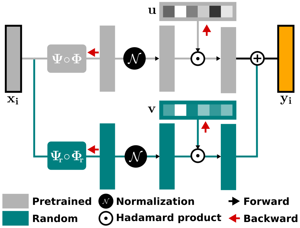
Figure 1: Given a word representation $x_{i}$, a BiLSTM ($\mathbf{\Phi}$) models the sequence, and a FC layer ($\bf\Psi$) performs classification. In standard fine-tuning, the units are pre-trained on a large source-dataset then adapted to the target one. In this work, we propose to add randomly initialised units (green branch) and jointly adapt them with pre-trained ones (gray branch). An element-wise sum is further applied to merge the two branches. Before merging, we balance the different behaviours of pre-trained and random units, using an independent normalisation ($\mathbfcal{N}$). Finally we let the network learn which of pre-trained or random neurons are more suited for every class, by adding learnable weighting vectors ($u$ and $v$ initialised with 1-values) on the FC layers.

One of the best approaches for POS tagging of social media text Meftah et al. (2018a), is transfer-learning, which relies on a neural-network learned on a source-dataset with sufficient annotated data, then further adapted to the problem of interest (target-dataset). While this approach is known to be very effective Zennaki et al. (2019), because it takes benefit from pre-trained neurons, it has one main drawback by design. Indeed, it has been shown in computer-vision Zhou et al. (2018a) that, when fine-tuning on scenes a model pre-trained on objects, it is the neuron firing on the white dog object that became highly sensitive to the white waterfall scene. Simply said, pre-trained neurons are biased by what they have learned in the source-dataset. This is also the case on NLP (see experiments). Consequently, pre-trained units struggle with learning patterns specific to the target-dataset (e.g., “wanna” or “gonna” in the Tweets domain). This last is non-desirable, since it has been shown recently Zhou et al. (2018b) that such specific units are important for performance. To overcome this drawback, one can propose to take benefit from randomly initialised units, that are by design non-biased. However, it is common to face small target-datasets that contain too few data to learn such neurons from scratch. Hence, in such setting, it is hard to learn random units that fire on specific patterns and generalise well.

In this article, we propose a hybrid method that takes benefit from both worlds, without their drawbacks. It consists in augmenting the source-network (set of pre-trained units) with randomly initialised units and jointly learn them. We call our method PretRand (Pretrained and Random units) and illustrate it in Fig. 1. The main difficulty is forcing the network to consider random units, because they have different behaviours than pre-trained ones. Indeed, while these last strongly fire discriminatively on many words, these first do not fire on any word at the initial stage of fine-tuning. Therefore, random units do not significantly contribute to the computation of gradients and are thus slowly updated. To overcome this problem, we proposed to independently normalise pre-trained and random layers. This last balances their range of activations and thus forces the network to consider them, both. Last but not least, we do not know which of pre-trained and random units are the best for every class-predictor, thus we propose to learn weighting vectors on top of each branch.

Evaluation was carried on 3 POS tagging Tweets datasets in a transfer-learning setting. Our method outperforms SOTA methods and significantly surpasses fairly comparable baselines.

2 Proposed Method: PretRand

2.1 Base Model

Given an input sentence $S$ $=$ $[w_{1},\ldots,w_{n}]$ of $n$ successive tokens $w_{i}$, the goal of a POS tagger is to predict the POS-tag $c_{i}$ $\in$ $\mathcal{C}$ of every $w_{i}$, with $\mathcal{C}$ $\in$ $\mathbb{R}^{C}$ being the tag-set. Hence, for our base model, we used a common sequence labelling model which first, computes for each token $w_{i}$, a word-level embedding (denoted $\mathbf{\Upsilon_{w}}$) and character-level embedding using biLSTM encoder ($\mathbf{\Upsilon_{c}}$), and concatenates them to get a final representation $x_{i}$. Second, it feeds the later representation into a biLSTM features extractor (denoted $\mathbf{\Phi}$) that outputs a hidden representation, that is itself fed into a fully-connected (FC) layer (denoted $\mathbf{\Psi}$) for classification. Formally, given $w_{i}$, the logits are obtained using: $\hat{y}_{w_{i}}=\mathbf{\Psi}\circ\mathbf{\Phi}\circ\mathbf{\Upsilon}(w_{i})$, with $\mathbf{\Upsilon}$ being the concatenation of the output of $\mathbf{\Upsilon_{c}}$ and $\mathbf{\Upsilon_{w}}$ for $w_{i}$. In a standard fine-tuning scheme Meftah et al. (2018b), $\mathbf{\Upsilon}$ and $\mathbf{\Phi}$ are pre-trained on the source-task and $\mathbf{\Psi}$ is randomly initialised. Then, the three modules are further jointly trained on the target-task by minimising a Softmax Cross-Entropy (SCE) loss using the SGD algorithm.

2.2 Adding Random Branch

As mentioned in the introduction, pre-trained neurons are biased by design, thus limited. This motivated our proposal to augment the pre-trained branch with additional random units (as illustrated in Fig. 1). To do so, theoretically one can add the new units in any layer of the base model. However in practice, we have to make a trade-off between performances and the number of parameters (model complexity). Thus, given that deep layers are more task-specific than shallow ones Peters et al. (2018); Mou et al. (2016), and that word embeddings (shallow layers) contain the majority of parameters, we choose to expand only the top layers. With this choice, we desirably increase the complexity of the model only by $1.02\times$ compared to the base one. In terms of the layers expanded, we specifically add $k$ units to $\mathbf{\Phi}$ resulting in an extra biLSTM layer: $\mathbf{\Phi_{r}}$ ($r$ for rand); and $C$ units in $\mathbf{\Psi}$ resulting in an extra FC layer: $\mathbf{\Psi_{r}}$. Hence, for every $w_{i}$, the additional random branch predicts class-probabilities following: $\hat{y}^{r}_{w_{i}}=\mathbf{\Psi_{r}}\circ\mathbf{\Phi_{r}}(x_{i})$ (with $x_{i}=\mathbf{\Upsilon}(w_{i})$). Note that, having two FC layers obviously outputs two predictions per class (one from the pre-trained FC $\hat{y}_{w_{i}}^{p}$ and one from the random $\hat{y}_{w_{i}}^{r}$), that thus need to be merged. Hence, to get the final predictions, we simply apply an element-wise sum between the output of both branches: $\hat{y}_{w_{i}}=\hat{y}_{w_{i}}^{p}\oplus\hat{y}_{w_{i}}^{r}$. As in the classical scheme, SCE is minimised but here, both branches are trained jointly.

2.3 Independent Normalisation

Nevertheless, while at the initial stage of fine-tuning, the pre-trained units are strongly firing on many words, the random ones are firing very weakly. As stated in some computer-vision works (Liu et al., 2015; Tamaazousti et al., 2018), the later setting causes an absorption of the weights, outputs and thus gradients of the random units by the pre-trained ones, which thus makes them useless at the end. We encountered the same problem with textual data on the POS-tagging problem. Indeed, as illustrated in the left plot of Fig.2, at the end of training, the distribution of the random units’ weights is still absorbed (closer to zero) by that of the pre-trained ones.

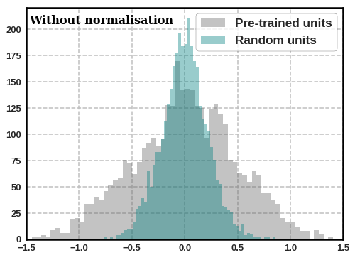
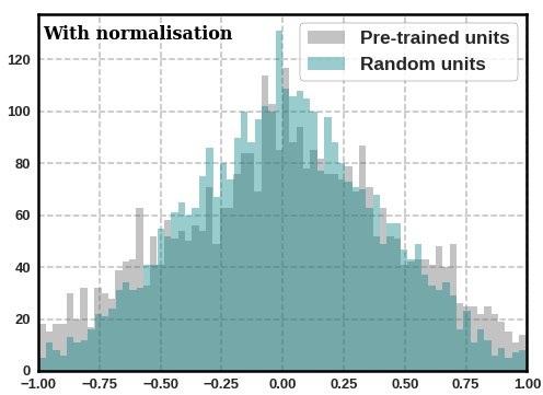
Figure 2: Distributions of learned weight-values for the randomly initialised (green) and pre-trained (gray) fully-connected layers after joint training. Left: without normalisation, right: with normalisation.

To prompt the two classifiers to work cooperatively, we normalise (using an $\ell_{p}$-norm) both of them independently before merging them. Formally, we apply $\mathbfcal{N}_{p}(x)$ $=$ $\frac{x}{||x||_{p}}$ on $\hat{y}_{w_{i}}^{p}$ and $\hat{y}_{w_{i}}^{r}$. The normalisation is desirably solving the weights absorption problem since at the end of the training, the distributions of the pre-trained and random weights become very similar (right of Fig. 2).

Furthermore, we have observed that despite the normalisation, the performances of the pre-trained classifiers were still much better than the randomly initialised ones. Thus, to make them more competitive, we propose to start with optimising only the randomly initialised units while freezing the pre-trained ones, then, launch the joint training. This is called random++ in the following.

2.4 Learnable Weighting Vectors

Back to the extra predictor (FC layer of random branch), it is important to note that both branches are equally important for making a decision for every class, i.e., no weight is applied on the dimensions of $\hat{y}_{w_{i}}^{p}$ and $\hat{y}_{w_{i}}^{r}$. However, this latter is sub-optimal since we, a priori, do not know which kind of units (random or pre-trained) is better for making a decision. Consequently, we propose to weight the contribution of the predictions for each class. For this end, instead of simply performing an element-wise sum between the random and pre-trained predictions, we first weight each of them with learnable weighting vectors, then compute a Hadamard product with their associated normalised predictions; the learnable vectors $u\in\mathbb{R}^{C}$ and $v\in\mathbb{R}^{C}$, respectively corresponding to the pre-trained and random branch, are initialised with 1-values and are learned by SGD. Formally, the final predictions are computed following: $\hat{y}_{w_{i}}=u\odot\mathbfcal{N}_{p}(\hat{y}_{w_{i}}^{p})\oplus v\odot\mathbfcal{N}_{p}(\hat{y}_{w_{i}}^{r})$.

3 Experiments

3.1 Implementation Details

In the word-level embeddings, tokens are lower-cased while the character-level component still retains access to the capitalisation information. We set the character embedding dimension at 50, the dimension of hidden states of the character-level biLSTM at 100 and used 300-dimensional word-level embeddings. The latter were pre-loaded from publicly available Glove pre-trained vectors on 42 billions words from a web crawling and containing 1.9M words Pennington et al. (2014). Note that, these embeddings are also updated during fine-tuning. For biLSTM (token-level feature extractor), we set the number of units of the pre-trained branch to 200 and experimented our approach with $k$ added random-units, with $k\in\{50,100,150,200\}$. For the normalisation, we used $\ell_{2}$-norm. Finally, in all experiments, training was performed using SGD with momentum and mini-batches of 8 sentences. Evidently, all the hyperparameters have been cross-validated.

3.2 Datasets

For the source-dataset, we used the Penn-Tree-Bank (PTB) of Wall Street Journal (WSJ), a large English dataset containing 1.2M+ tokens from the newswire domain annotated with the PTB tag-set. Regarding the target-datasets, we used three datasets in the Tweets domain: TPoS (Ritter et al., 2011), annotated with 40 tags ; ARK Owoputi et al. (2013) containing 25 coarse tags; and the recent TweeBank Liu et al. (2018) containing 17 tags (PTB universal tag-set). The number of tokens in the datasets are given in Table 1.

Corpus	TPoS	Ark	TweeBank
Train	10,652	26,594	24,753
Dev	2,242	n/a	11,742
Test	2,291	7,707	19,112

Table 1: Number of tokens in every used dataset.

Method	#params	TPoS		ArK	TweeBank
		Dev	Test	Test	Dev	Test	Avg
GATE (Derczynski et al., 2013)	n/a	89.37	88.69	n/a	n/a	n/a	n/a
GATE-bootstrap (Derczynski et al., 2013)	n/a	n/a	90.54	n/a	n/a	n/a	n/a
ARK (Owoputi et al., 2013)	n/a	n/a	90.40	93.2	n/a	94.6	n/a
TPANN (Gui et al., 2017)	n/a	91.08	90.92	92.8	n/a	n/a	n/a
Random-200	$1\times$	88.32	87.76	90.67	91.20	91.56	89.90
Random-400	$1.03\times$	89.01	88.89	90.99	91.38	91.63	90.38
Standard fine-tuning	$1\times$	90.96	90.7	91.72	92.59	92.99	91.79
Ensemble Model (2 rand)	$2\times$	89.20	88.8	91.36	91.73	92.05	90.62
Ensemble Model (1 pret + 1 rand)	$2\times$	89.77	88.61	91.41	92.57	92.85	91.04
PretRand (Ours)	$1.02\times$	91.56	91.46	93.77	94.51	94.95	93.24

Table 2: Comparison of our method to state-of-the-art (top) and baselines (bottom) in terms of token-level accuracy (in %) on 3 Tweets datasets. Note that, baselines are more fairly comparable to our method. In the second and last columns, we respectively highlighted the number of parameters and the average performance on the 3 datasets.

3.3 Comparison Methods

To assess the POS tagging performances of our PretRand model, we compared it to 5 baselines: Random-200 and Random-400: randomly initialised neural model with 200 and 400 biLSTM’s units; Fine-tuning: pre-trained neural model, fine-tuned with the standard scheme; Ensemble (2 rand): averaging the predictions of two base models randomly initialised and learned independently (with different random initialisation) on Tweets datasets; and Ensemble (1 pret + 1 rand): same as the previous but with one pre-trained on WSJ and the other randomly initialised.

We also compared it to the 3 best SOTA methods: Derczynski et al. (2013) (GATE) is a model based on HMMs with a set of normalisation rules, external dictionaries and lexical features. They experiment it on TPoS, with WSJ and 32K tokens from the NPS IRC corpus. They also used 1.5M additional training tokens annotated by vote-constrained bootstrapping (GATE-bootstrap). Owoputi et al. (2013) proposed a model based on first-order Maximum Entropy Markov Model (MEMM) with greedy decoding and using brown clustering and careful hand-engineered features. Recently, Gui et al. (2017) proposed TPANN that uses adversarial training to leverage huge amounts of unlabelled Tweets.

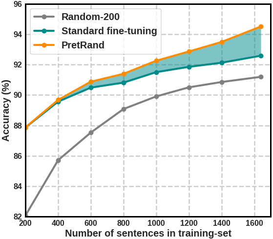
Figure 3: Performances (on dev-set of TweeBank) according different training-set sizes for the target-dataset. Transparent green highlights the difference between our PretRand and standard fine-tuning.

Method	TPoS	ArK	TweeBank	Avg
PretRand	91.46	93.77	94.95	93.39
-learnVect	91.25	93.46	94.59	93.10
-random++	90.97	93.11	94.13	92.73
-l2 norm	90.76	92.11	93.38	92.08

Table 3: Ablation study, Token level accuracy (in %) when progressively ablating PretRand components.

3.4 Results

From the results given in Table 2, one can first see that our approach outperforms the SOTA and baseline methods on all the datasets. More interestingly, PretRand significantly outperforms the popular fine-tuning baseline by +1.4% absolute point on average and is better on all classes (see per-class improvement on Fig. 4). PretRand also outperforms the challenging Ensemble Model by a large margin (+2.2%), while using much less parameters. This clearly highlights the difference of our method with ensemble methods and the importance of having a shared word representation as well as our normalisation and weighting learnable vectors during training. A key asset of PretRand, is that it uses only 0.02% more parameters compared to the fine-tuning baseline.

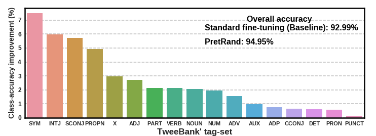
Figure 4: Sorted class-accuracy improvement (%) on TweeBank of PretRand compared to fine-tuning.

An interesting experiment is to evaluate the gain of performance of PretRand compared to fine-tuning, according different target-datasets’ sizes. From the results in Fig. 3, PretRand has desirably a bigger gain with bigger target-task datasets, which clearly means that the more target training-data, the more interesting our method will be.

To assess the contribution of different components of PretRand, we performed an ablation study. Specifically, we successively ablated the main components of PretRand, namely, the learnable vectors (learnVect), the longer training for random units (random++) and the normalisation ($\ell_{2}$-norm). From the results in Table 3, we can observe that the performances are only marginally better than standard fine-tuning when ablating the three components from PretRand. More importantly, adding each of them successively, makes the performances significantly better, which highlights the importance of every component.

4 Analysis

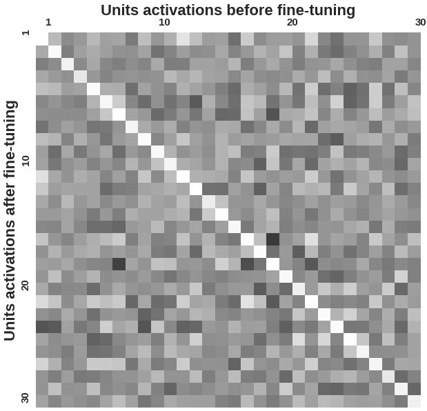
Figure 5: Correlation between units’ activations before fine-tuning (columns) and after fine-tuning (rows).

Bias when fine-tuning pre-trained units
Here our goal is to highlight that as in Zhou et al. (2018a), pre-trained units can be biased in the standard fine-tuning scheme. To do so, we follow Tamaazousti et al. (2017) and analyse the units of $\mathbf{\Phi}$ (biLSTM layer) before and after fine-tuning. Specifically, we compute the Pearson’s correlation between all the units of the layer before and after fine-tuning. Here, a unit is represented by the random variable being the concatenation of its output activations from all the validation samples of the TweeBank dataset. From the resulting correlation matrix illustrated in Fig. 5, one can clearly observe the white diagonal, highlighting the fact that, every unit after fine-tuning is more correlated with itself before fine-tuning than with any other unit. This clearly confirms our initial motivation that pre-trained units are highly biased to what they have learned in the source-dataset, making them limited to learn patterns specific to the target-dataset.

Additionally, we visualise in Fig. 6 a concrete example of a biased neuron when transferring from newswire to Tweets domain. Specifically, we show the top-10 words activating unit-169 of $\mathbf{\Phi}$ (from the standard fine-tuning baseline), before fine-tuning (at this stage, the model is trained on the source-dataset WSJ) and during fine-tuning on the TweeBank dataset. We can observe that this unit is highly sensitive to proper nouns (e.g., George and Washington) before fine-tuning, and to words with capitalised first-letter whether the word is a proper noun or not (e.g., Man and Father) during fine-tuning on TweeBank dataset. Indeed, we found that most of tokens with upper-cased first letter are mistakenly predicted as proper nouns (PROPN) in the standard fine-tuning scheme. In fact, in standard English, inside sentences, only proper nouns start with upper-cased letter thus fine-tuning the pre-trained model fails to slough this pattern which is not always respected in Tweets.

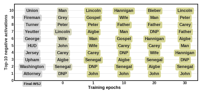
Figure 6: Top-10 words activating unit-169 of standard fine-tuning scheme, before fine-tuning (Final-WSJ) and during fine-tuning on TweeBank.

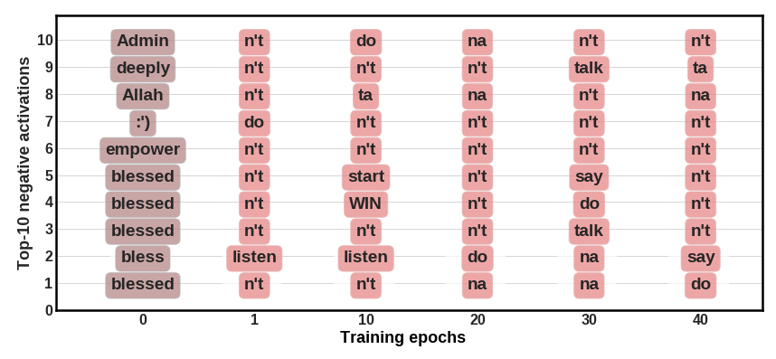
Figure 7: Top-10 words activating unit-99 of the random branch of PretRand, before and during training.

Unique units emerge in random branch
Finally, we highlight the ability of randomly initialised units to learn patterns specific to the target-dataset and not learned by the pre-trained ones because of their bias problem. To do so, we visualise unique units – i.e., random units having a correlation lower than 0.4 with pre-trained ones – emerging in the random branch. While only one shown in Fig. 7, many unique units have been learned by the random branch of our PretRand model: 37.5% of the 200 random units have correlation lower than 0.4 with the pre-trained ones. Regarding unit-99, it is highly discriminative to tokens ”na”, ”ta” and ”n’t”. Indeed, in TweeBank, words like ”gonna” (going to) are tokenized into two tokens: ”gon” and ”na”, with the later annotated as a particle and the former as a verb. Importantly, not even one unit from the standard fine-tuning scheme has been found firing on the same important and target-dataset specific pattern.

5 Conclusion

In this paper, we introduced a method to improve fine-tuning using 3 main ideas: adding random units and jointly learn them with pre-trained ones; normalising the activations of both to balance their different behaviours; applying learnable weights on both predictors to let the network learn which of random or pre-trained one is better for every class. We have demonstrated its effectiveness on domain adaptation from newswire domain to three commonly used Tweets-datasets for POS tagging.

References

- Derczynski et al. (2013) Leon Derczynski, Alan Ritter, Sam Clark, and Kalina Bontcheva. 2013. Twitter part-of-speech tagging for all: Overcoming sparse and noisy data. In RANLP 2013, pages 198–206.
- Gui et al. (2017) Tao Gui, Qi Zhang, Haoran Huang, Minlong Peng, and Xuanjing Huang. 2017. Part-of-speech tagging for twitter with adversarial neural networks. In EMNLP, pages 2411–2420.
- Liu et al. (2015) Wei Liu, Andrew Rabinovich, and Alexander C Berg. 2015. Parsenet: Looking wider to see better. arXiv preprint arXiv:1506.04579.
- Liu et al. (2018) Yijia Liu, Yi Zhu, Wanxiang Che, Bing Qin, Nathan Schneider, and Noah A Smith. 2018. Parsing tweets into universal dependencies. In NAACL, volume 1, pages 965–975.
- Meftah et al. (2018a) Sara Meftah, Nasredine Semmar, and Fatiha Sadat. 2018a. A neural network model for part-of-speech tagging of social media texts. In LREC.
- Meftah et al. (2018b) Sara Meftah, Nasredine Semmar, Fatiha Sadat, and Stephan Raaijmakers. 2018b. Using neural transfer learning for morpho-syntactic tagging of south-slavic languages tweets. In VarDial 2018, pages 235–243.
- Mou et al. (2016) Lili Mou, Zhao Meng, Rui Yan, Ge Li, Yan Xu, Lu Zhang, and Zhi Jin. 2016. How transferable are neural networks in nlp applications? In EMNLP, pages 479–489.
- Niehues and Cho (2017) Jan Niehues and Eunah Cho. 2017. Exploiting linguistic resources for neural machine translation using multi-task learning. In Proceedings of the Second Conference on Machine Translation, pages 80–89.
- Owoputi et al. (2013) Olutobi Owoputi, Brendan O’Connor, Chris Dyer, Kevin Gimpel, Nathan Schneider, and Noah A Smith. 2013. Improved part-of-speech tagging for online conversational text with word clusters. In NAACL, pages 380–390.
- Pennington et al. (2014) Jeffrey Pennington, Richard Socher, and Christopher Manning. 2014. Glove: Global vectors for word representation. In Proceedings of the 2014 conference on empirical methods in natural language processing (EMNLP), pages 1532–1543.
- Peters et al. (2018) Matthew Peters, Mark Neumann, Mohit Iyyer, Matt Gardner, Christopher Clark, Kenton Lee, and Luke Zettlemoyer. 2018. Deep contextualized word representations. In NAACL, volume 1, pages 2227–2237.
- Ritter et al. (2011) Alan Ritter, Sam Clark, Oren Etzioni, et al. 2011. Named entity recognition in tweets: an experimental study. In EMNLP, pages 1524–1534. Association for Computational Linguistics.
- Semmar et al. (2008) Nasredine Semmar, Laib Meriama, and Christian Fluhr. 2008. Evaluating a natural language processing approach in arabic information retrieval. In ELRA Workshop on Evaluation Looking into the Future of Evaluation: When automatic metrics meet task-based and performance-based approaches, page 24.
- Tamaazousti et al. (2017) Youssef Tamaazousti, Hervé Le Borgne, and Céline Hudelot. 2017. Mucale-net: Multi categorical-level networks to generate more discriminating features. In CVPR.
- Tamaazousti et al. (2018) Youssef Tamaazousti, Hervé Le Borgne, Céline Hudelot, Mohamed El Amine Seddik, and Mohamed Tamaazousti. 2018. Learning more universal representations for transfer-learning. arXiv:1712.09708.
- Zennaki et al. (2019) O Zennaki, N Semmar, and Laurent Besacier. 2019. A neural approach for inducing multilingual resources and natural language processing tools for low-resource languages. Natural Language Engineering, 25(1):43–67.
- Zhou et al. (2018a) Bolei Zhou, David Bau, Aude Oliva, and Antonio Torralba. 2018a. Interpreting deep visual representations via network dissection. IEEE Transactions on Pattern Analysis and Machine Intelligence.
- Zhou et al. (2018b) Bolei Zhou, Yiyou Sun, David Bau, and Antonio Torralba. 2018b. Revisiting the importance of individual units in cnns via ablation. arXiv preprint arXiv:1806.02891.