Skewness of nuclear matter and three-particle correlations

Abstract

We present a study of the skewness of nuclear matter, which is proportional to the third derivative of the energy per nucleon with respect to the baryon density at the saturation point, in the framework of the Landau-Migdal theory. We derive an exact relation between the skewness, the nucleon effective mass, and two-particle and three-particle interaction parameters. We also present qualitative estimates, which indicate that three-particle correlations play an important role for the skewness.

PhySH: Nuclear matter; Nuclear forces; Nuclear many-body theory.

I INTRODUCTION

The properties of infinite nuclear matter have been the subject of intensive investigations for many decades, mainly because of the wide range of applications, including the properties of heavy nuclei and their excitation modes Blaizot (1980); Mahaux et al. (1985), heavy ion collisions Danielewicz et al. (2002), the physics of supernova explosions Bethe (1990); Lattimer (2012), and neutron stars Baym et al. (2018). Besides the binding energy per nucleon and the saturation density, other basic properties of nuclear matter like the effective mass of nucleons and its momentum dependence Li et al. (2018), the incompressibility Piekarewicz (2010), the symmetry energy and its density dependence Zhang and Chen (2013), and recently the skewness Cai and Chen (2017), provide basic information on the effective interaction between nucleons in the medium. Theoretical descriptions of those and other important properties of nuclear matter have been based on Brückner’s G-matrix approach Bethe et al. (1963); Rajaraman (1963); Brown (1971), relativistic theories based on meson exchange Serot and Walecka (1986); Müller and Serot (1995); Meng et al. (2016), effective interactions of the Skyrme Zhang and Chen (2016) and Landau-Migdal type Speth et al. (2014), and effective field theories Kaplan et al. (1998); Hammer and Furnstahl (2000); Steele (2000); Bogner et al. (2010); Holt et al. (2018).

In this article we focus our attention on the skewness of nuclear matter and its implication for three-particle correlations. Skewness is defined as $J=27\rho^{3}\left({\rm d}^{3}E_{A}/{\rm d}\rho^{3}\right)$ at $\rho=\rho_{0}$, where $E_{A}$ is the energy per nucleon in isospin symmetric nuclear matter, $\rho$ is the baryon density, and $\rho_{0}$ is the saturation density ($\rho_{0}=0.15$ fm^-3). This physical quantity has been receiving interest in connection to phenomenological applications of the liquid drop model to heavy nuclei Pearson (1991), and relativistic approaches to nuclear matter Kouno et al. (1995); Frohlich et al. (1998). Recently, empirical values have been extracted in Refs. Steiner et al. (2010); Cai and Chen (2017) from flow data in heavy ion collisions and neutron star observations. Based on the analogy to the incompressibility, which is defined as $K=9\rho^{2}\left({\rm d}^{2}E_{A}/{\rm d}\rho^{2}\right)$ at $\rho=\rho_{0}$, and which is known to be related to the spin-isospin averaged two-particle interaction in the medium Migdal (1967); Migdal et al. (1990); Kamerdzhiev et al. (2004), one may expect that $J$ is related to the spin-isospin averaged three-particle interaction. The aim of this paper is to work out this relation in detail and to discuss the result in connection to empirical values. To achieve this we will use the framework of the Landau-Migdal theory of nuclear matter Migdal (1967); Migdal et al. (1990), which is based on Landau’s Fermi liquid theory Landau (1956, 1957, 1959); Baym and Pethick (2004). The main advantage of this theory is that symmetries, like gauge invariance and Galilei invariance (or Lorentz invariance in its relativistic extension Baym and Chin (1976)) are incorporated rigorously, and that the description of collective excitations of the system is physically very appealing Nozières (1964); Negele and Orland (1998). However, to the best of our knowledge, the theory has not yet been applied to directly relate the skewness of nuclear matter to three-particle interactions. It is well known that the effects of three-particle interactions can be incorporated by using effective density-dependent two-particle interactions Ring and Schuck (1980), and this approach has been used in many recent studies with Skyrme-type interactions Chen et al. (2009). However, in view of the long history of studies on three-particle correlations in nuclear matter Bethe (1965); Day (1981); Fritsch et al. (2005), it is desirable to know a more direct relation of a physical quantity, which is connected to observables, to three-particle interaction parameters.

In Sec. II we derive the relation between the skewness of nuclear matter and the three-particle Landau-Migdal parameters, which are defined in a similar way as the familiar two-particle parameters. In Sec. III we discuss this relation in connection to empirical values, and in Sec. IV we present further qualitative discussions, which indicate that three-particle correlations play an important role for the skewness. A summary is presented in Sec. V, and additional details are collected in the Appendices.

II THEORETICAL FRAMEWORK

Here we discuss the form of the first three derivatives of the energy density, $E(\rho)$, of spin saturated isospin symmetric nuclear matter w.r.t. the baryon density $\rho=2\,p_{F}^{3}/(3\pi^{2})$, where $p_{F}$ is the Fermi momentum. Extending Landau’s formula Landau (1956, 1957, 1959); Baym and Pethick (2004) for the variation of $E$ w.r.t. spin-isospin independent deviations of the quasiparticle occupation numbers from a reference Fermi distribution (corresponding to a density $\rho_{0}=2\,p_{F0}^{3}/(3\pi^{2})>0$) to include the third order term, we can write

$$\delta E(\rho) =4\int\frac{{\rm d}^{3}k}{(2\pi)^{3}}\ \varepsilon(\bm{k};\rho_{0})\,\delta n_{\bm{k}}$$

$$+\frac{1}{2}\left(\prod_{i=1}^{2}\,4\int\frac{{\rm d}^{3}k_{i}}{(2\pi)^{3}}\,\delta n_{\bm{k}_{i}}\right)\,f(\bm{k}_{1},\bm{k}_{2};\rho_{0})$$

$$+\frac{1}{6}\left(\prod_{i=1}^{3}\,4\int\frac{{\rm d}^{3}k_{i}}{(2\pi)^{3}}\,\delta n_{\bm{k}_{i}}\right)\,h(\bm{k}_{1},\bm{k}_{2};\bm{k}_{3};\rho_{0}).$$ (1)

Here $\varepsilon(\bm{k};\rho)$ is the energy of a quasiparticle with momentum $\bm{k}$; $f(\bm{k}_{1},\bm{k}_{2};\rho)$ is the spin-isospin averaged forward scattering amplitude of two quasiparticles with momenta $\bm{k}_{1},\bm{k}_{2}$; and $h(\bm{k}_{1},\bm{k}_{2};\bm{k}_{3};\rho)$ is the spin-isospin averaged three-particle forward scattering amplitude. The amplitudes $f$ and $h$ are totally symmetric with respect to interchanges of the momentum variables, and can be represented by a set of connected diagrams with four and six external nucleon lines, respectively. Besides the momentum variables, we also indicate the dependence on the background density explicitly.

The form of $\delta n_{\bm{k}}$ corresponding to a change of the Fermi momentum ($p_{F0}\rightarrow p_{F}$) is independent of the direction of $\bm{k}$ and given, to first order in $(p_{F}-p_{F0})$, by

$$\delta n_{k}=\left(p_{F}-p_{F0}\right)\,\delta(p_{F0}-k)\,.$$ (2)

The corresponding first order variation of $E$ is given by

$$\delta E=4\int\frac{{\rm d}^{3}k}{(2\pi)^{3}}\varepsilon(\bm{k};\rho_{0})\,\delta n_{k}=\varepsilon(p_{F0};\rho_{0})\,\cdot\,\delta\rho\,,$$ (3)

where $\delta\rho=\frac{2p_{F0}^{2}}{\pi^{2}}\cdot(p_{F}-p_{F0})$. Because the reference density $\rho_{0}>0$ is arbitrary, we get the well known result Hugenholtz and van Hove (1958)

$$\frac{{\rm d}E(\rho)}{{\rm d}\rho}=\varepsilon(p_{F};\rho)\,.$$ (4)

Next we consider the first order variation of the quasiparticle energy:

$$\delta\varepsilon({k}_{1};\rho) =4\int\frac{{\rm d}^{3}k_{2}}{(2\pi)^{3}}\,f(\bm{k}_{1},\bm{k}_{2};\rho_{0})\,\delta n_{{k}_{2}}$$

$$=f_{0}(k_{1},p_{F0};\rho_{0})\,\cdot\,\delta\rho\,,$$ (5)

where the $\ell=0$ two-particle forward scattering amplitude, which is proportional to the $s$-wave scattering length in the medium, is the angular average of $f({\bm{k}_{1}},{\bm{k}_{2}};\rho)$. The definition, together with the $\ell=1$ amplitude which will be used below, is

$$\frac{1}{2\ell+1}\,f_{\ell}(k_{1},k_{2};\rho)=\int\frac{{\rm d}\Omega_{2}}{4\pi}\,\left({\bm{\hat{k}}}_{1}\cdot{\bm{\hat{k}}}_{2}\right)^{\ell}\,f({\bm{k}_{1}},{\bm{k}_{2}};\rho),$$ (6)

where $\ell=0,1$, and we use the notation ${{\rm d}\Omega_{i}\equiv{\rm d}\Omega_{\bm{k}_{i}}}$. From Eq. (5) we obtain the partial derivative of the quasiparticle energy w.r.t. the density as

$$\frac{\partial\varepsilon(k_{1};\rho)}{\partial\rho}=f_{0}(k_{1},k_{2}=p_{F};\rho)\,.$$ (7)

For the total derivative of the Fermi energy (chemical potential) w.r.t. the density we then obtain the well known result Negele and Orland (1998)

$$\frac{{\rm d}\varepsilon(p_{F};\rho)}{{\rm d}\rho}=\frac{{\rm d}^{2}E}{{\rm d}\rho^{2}}=v(p_{F};\rho)\,\frac{\pi^{2}}{2p_{F}^{2}}+f_{0}(p_{F},p_{F};\rho)$$

$$\equiv\frac{\pi^{2}}{2p_{F}M^{*}(p_{F};\rho)}+f_{0}(p_{F},p_{F};\rho)\equiv\frac{\pi^{2}}{2p_{F}M^{*}}\left(1+F_{0}\right).$$ (8)

Here $v(k;\rho)={\rm\partial}\varepsilon(k;\rho)/{\rm\partial}k$ is the magnitude of the velocity of the quasiparticle, and we introduced the momentum dependent effective nucleon mass (Landau effective mass) $M^{*}(k;\rho)$ by

$$v(k;\rho)\equiv\frac{k}{M^{*}(k;\rho)}\,.$$ (9)

In the last relation of Eq. (8) we defined the dimensionless Landau-Migdal parameters as

$$F_{\ell}=\frac{2p_{F}M^{*}}{\pi^{2}}\,f_{\ell}\,.$$ (10)

Before proceeding to the third order derivative, we note that the effective mass is related to the $\ell=1$ two-particle forward scattering amplitude by

$$\frac{k}{M^{*}(k;\rho)}+\frac{2p_{F}^{2}}{3\pi^{2}}f_{1}(k,p_{F};\rho)=\frac{k}{M}\,,$$ (11)

which for $k=p_{F}$ becomes the familiar Landau effective mass relation Landau (1956, 1957, 1959); Nozières (1964).

Next we consider the derivative of Eq. (8) w.r.t. the density, which gives

$$\frac{{\rm d}^{3}E}{{\rm d}\rho^{3}}=-\frac{\pi^{4}}{4p_{F}^{4}M^{*}}-\frac{\pi^{2}}{2p_{F}M^{*2}}\frac{{\rm d}M^{*}}{{\rm d}\rho}+\frac{{\rm d}f_{0}}{{\rm d}\rho}\,.$$ (12)

By using the derivative of Eq. (7) w.r.t. $k_{1}$, we can write

$$\frac{\partial M^{*}}{\partial\rho}=-\frac{M^{*2}}{2p_{F}}\frac{\partial f_{0}}{\partial p_{F}}\,.$$ (13)

Recall (see footnote 1) that the quantity $\partial f_{\ell}/\partial p_{F}$ actually means

$$\frac{\partial f_{\ell}}{\partial p_{F}}\equiv\left[\left(\frac{\partial}{\partial k_{1}}+\frac{\partial}{\partial k_{2}}\right)f_{\ell}(k_{1},k_{2};\rho)\right]_{k_{1}=k_{2}=p_{F}}\,,$$

and because of the symmetry of the 2-particle amplitude this is the same as the derivative w.r.t. only one momentum variable, multiplied by $2$. Further we note that, from Eq. (1), a change of the Fermi momentum leads to the following first order variation of the two-particle scattering amplitude:

$$\delta f(\bm{k}_{1},\bm{k}_{2};\rho) =4\int\frac{{\rm d}^{3}k_{3}}{(2\pi)^{3}}\,h(\bm{k}_{1},\bm{k}_{2},\bm{k}_{3};\rho_{0})\,\delta n_{{k}_{3}}$$

$$=\delta\rho\,\cdot\,\int\frac{{\rm d}\Omega_{3}}{4\pi}\,h(\bm{k}_{1},\bm{k}_{2},\bm{k}_{3};\rho_{0})|_{k_{3}=p_{F0}}\,.$$ (14)

By taking the $\ell=0,1$ moments of this relation, we obtain

$$\frac{\partial}{\partial\rho}\,f_{\ell}(k_{1},k_{2};\rho)=h_{\ell}(k_{1},k_{2},k_{3}=p_{F};\rho)\,,$$ (15)

where the $\ell=0,1$ three-particle amplitudes are defined by

$$\frac{1}{2\ell+1}h_{\ell}(k_{1},k_{2},k_{3};\rho)$$

$$\hskip 28.45274pt=\int\frac{{\rm d}\Omega_{2}}{4\pi}\,\int\frac{{\rm d}\Omega_{3}}{4\pi}\,\left(\bm{\hat{k}}_{1}\cdot\bm{\hat{k}}_{2}\right)^{\ell}h(\bm{k}_{1},\bm{k}_{2},\bm{k}_{3};\rho)\,.$$ (16)

Substituting Eqs. (13) and (15) into Eq. (12) gives

$$\frac{{\rm d}^{3}E}{{\rm d}\rho^{3}}=-\frac{\pi^{4}}{4p_{F}^{4}M^{*}}+\frac{3\pi^{2}}{4p_{F}^{2}}\frac{\partial f_{0}}{\partial p_{F}}-\frac{\pi^{4}}{4p_{F}^{3}M^{*2}}\frac{\partial M^{*}}{\partial p_{F}}+h_{0}\,.$$ (17)

In order to eliminate the derivative of $f_{0}$ from this equation, we take the partial derivative w.r.t. the density on both sides of Eq. (11), and then set $k=p_{F}$. Using again Eq. (13) we obtain

$$p_{F}\,\frac{\partial}{\partial p_{F}}\left(f_{0}+\frac{1}{3}f_{1}\right)+\frac{4}{3}f_{1}+\frac{4p_{F}^{3}}{3\pi^{2}}\,h_{1}=0\,.$$ (18)

As explained in App. A, this relation can also be derived directly from the Galilei invariance of the two-particle scattering amplitude. The $f_{1}$ terms in Eq. (18) can be expressed by the effective mass, by using Eq. (11) and its derivative w.r.t. $k$ at the Fermi surface. In this way we can rewrite Eq. (18) as

$$p_{F}\frac{\partial f_{0}}{\partial p_{F}}-\frac{3\pi^{2}}{p_{F}}\frac{M-M^{*}}{MM^{*}}+\frac{\pi^{2}}{M^{*2}}\frac{\partial M^{*}}{\partial p_{F}}+\frac{4p_{F}^{3}}{3\pi^{2}}\,h_{1}=0\,.$$ (19)

Using this relation to eliminate the derivative of $f_{0}$ from Eq. (17) we finally obtain

$$\frac{{\rm d}^{3}E}{{\rm d}\rho^{3}}=\frac{3\pi^{4}}{4p_{F}^{4}M^{*}}$$

$$\hskip 14.22636pt\times\left(-\frac{1}{3}+3\frac{M-M^{*}}{M}-\frac{4}{3}\frac{p_{F}}{M^{*}}\,\frac{\partial M^{*}}{\partial p_{F}}+\left(H_{0}-H_{1}\right)\right)\,.$$ (20)

Here we have defined the dimensionless three-particle interaction parameters by

$$H_{\ell} =\left(\frac{2p_{F}M^{*}}{\pi^{2}}\rho\right)\,h_{\ell}=\frac{4p_{F}^{4}M^{*}}{3\pi^{4}}\,h_{\ell}\,.$$ (21)

One should note that Eq. (20) is an exact relation.

III DISCUSSION ON EMPIRICAL VALUES

In order to connect the relations of Sec. II to empirical values, we note that the energy per nucleon ($E_{A}$) is related to the energy density ($E$) by

$$E_{A}(\rho)=E(\rho)/\rho\,.$$ (22)

All the relations which follow will be given for $\rho=\rho_{0}$, where $\rho_{0}$ is the saturation density defined by $\left.{\rm d}E_{A}/{\rm d}\rho\right|_{\rho=\rho_{0}}=0$.

Taking the first derivative of Eq. (22) and using Eq. (4) we obtain the well known relation $E_{A}(\rho)=\varepsilon(p_{F};\rho)$ Hugenholtz and van Hove (1958). The second derivative of Eq. (22) and its relation to the incompressibility ($K$) of nuclear matter is given by Cai and Chen (2017); Li et al. (2018)

$$\frac{{\rm d}^{2}E_{A}}{{\rm d}\rho^{2}}=\frac{1}{\rho}\frac{{\rm d}^{2}E}{{\rm d}\rho^{2}}\equiv\frac{K}{9\rho^{2}}\,.$$ (23)

The third derivative of Eq. (22) and its relation to the skewness ($J$) of nuclear matter is given by Cai and Chen (2017); Li et al. (2018)

$$\frac{{\rm d}^{3}E_{A}}{{\rm d}\rho^{3}}=-\frac{3}{\rho^{2}}\frac{{\rm d}^{2}E}{{\rm d}\rho^{2}}+\frac{1}{\rho}\frac{{\rm d}^{3}E}{{\rm d}\rho^{3}}\equiv\frac{J}{27\rho^{3}}\,.$$ (24)

By using Eqs. (8) and (20), the incompressibility and the skewness can be expressed as

$$K =\frac{3p_{F}^{2}}{M^{*}}\,\left(1+F_{0}\right)\,,$$ (25)

$$J =-9K+\frac{9p_{F}^{2}}{M^{*}}$$

$$\times\left(-\frac{1}{3}+3\frac{M-M^{*}}{M}-\frac{4}{3}\,\frac{p_{F}}{M^{*}}\,\frac{\partial M^{*}}{\partial p_{F}}+\left(H_{0}-H_{1}\right)\right)\,.$$ (26)

Recent analyses Cai and Chen (2017); Li et al. (2018) which take into account constraints from heavy ion collisions and astrophysical observations, suggest the following ranges of $K$ and $J$ at the saturation density $\rho_{0}=0.15$ fm^-3:

$$0.20\,[{\rm GeV}]\,<\,\, K\,<\,\,0.30\,[{\rm GeV}],$$ (27)

$$-0.50\,[{\rm GeV}]\,<\,\, J\,<\,\,-0.01\,[{\rm GeV}].$$ (28)

From these values and Eqs. (25) and (26) we can make a few observations: First, the Fermi gas value of the incompressibility $K_{\rm free}=3\frac{p_{F}^{2}}{M}\simeq 0.22$ GeV is inside the range of Eq. (27), i.e., the detailed values of $M^{*}$ and $F_{0}$ result in fine-tuning of $K$ but do not lead to order of magnitude changes. On the other hand, the Fermi gas value for the skewness $J_{\rm free}=-10K_{\rm free}\simeq-2.2$ GeV is very large in magnitude compared to the empirical values of Eq. (28), indicating that some of the correction terms in Eq. (26) must be large and positive. In fact, by using the lower limits of Eqs. (27) and (28), we see that Eq. (26) implies

$$\frac{8}{3}\,\frac{M-M^{*}}{M^{*}}-\frac{4}{3}\frac{p_{F}M}{M^{*2}}\frac{\partial M^{*}}{\partial p_{F}}+\frac{M}{M^{*}}\left(H_{0}-H_{1}\right)>2.38.$$ (29)

The value of the effective mass at the saturation density of symmetric nuclear matter has been the subject of intensive investigations during the last decades Mahaux et al. (1985); Li et al. (2018), and most of them are consistent with the range

$$0.7\,<\,\frac{M^{*}}{M}\,<\,\,1.0.$$ (30)

The momentum dependence of the effective mass has been intensively studied by Mahaux et al. Mahaux et al. (1985). Their studies, as well as subsequent work of Blaizot et al. Blaizot and Friman (1981), indicate that $M^{*}(k;\rho)$ has a pronounced peak very close to the Fermi surface (i.e., $\partial M^{*}/\partial p_{F}\simeq 0$), and it was shown that this behavior comes mainly from the same polarization effects which cause an imaginary part of the single particle energy away from the Fermi surface. More recent studies van Dalen et al. (2005) indicate that this peak of the effective mass may be slightly above the Fermi surface, i.e., $M^{*}(k;\rho)$ is still increasing at $k=p_{F}$ before it reaches a maximum. In our subsequent estimates we will therefore assume that $\partial M^{*}/\partial p_{F}>0$. We then obtain an upper limit for the first two terms in Eq. (29):

$$\frac{8}{3}\,\frac{M-M^{*}}{M^{*}}-\frac{4}{3}\frac{p_{F}M}{M^{*2}}\frac{\partial M^{*}}{\partial p_{F}}<1.14.$$ (31)

By comparing Eqs. (29) and (31) we clearly see that one needs a large positive contribution from the three-body terms in order to explain the empirical values:

$$\frac{M}{M^{*}}\left(H_{0}-H_{1}\right)>1.24.$$ (32)

IV QUALITATIVE DISCUSSIONS ON THE THREE-PARTICLE AMPLITUDE

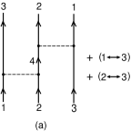
Figure 1: (a) Lowest order diagram contributing to the two-particle correlation piece $h^{\rm(2pc)}$. (b) An example of a contribution to the three-particle correlation piece $h^{\rm(3pc)}$. In each case the solid lines are nucleons, and the dashed lines denote the nuclear potential, which is assumed to be antisymmetrized according to Eq. (35).

The three-particle amplitude $h(\bm{k}_{1},\bm{k}_{2},\bm{k}_{3};\rho)$ contains 1-particle reducible pieces, i.e., diagrams which can be made disconnected by cutting a single intermediate nucleon line, and 1-particle irreducible pieces. In perturbation theory, the former ones start with terms of second order in the nuclear potential, see Fig. 1(a). We will refer to them as the “two-particle correlation” (2pc) contributions to the three-particle amplitude. On the other hand, the 1-particle irreducible pieces start with third order perturbation theory, and involve interactions between all three pairs of the particles. (See Fig. 1(b) for an example.) We will call them the “three-particle correlations” (3pc). We therefore split the three-particle amplitude as follows:

$$h=h^{(\rm 2pc)}+h^{(\rm 3pc)}\,.$$ (33)

The expression for the lowest order process shown in Fig. 1(a) can be derived from the definition given in Eq. (1) by taking the second functional derivative of the energy density in second order perturbation theory. Those familiar relations Brown (1971); Negele and Orland (1998) are summarized in App. B, and the second (2nd) order result for $h$ is

$$h^{(\rm 2nd)}(\bm{k}_{1},\bm{k}_{2},\bm{k}_{3};\rho)=\sum_{4}\delta_{\bm{k}_{1}+\bm{k}_{2},\bm{k}_{3}+\bm{k}_{4}}$$

$$\hskip 36.98857pt\times P\,\frac{|\langle 12|\,\hat{v}\,|34\rangle_{a}|^{2}}{\epsilon_{3}+\epsilon_{4}-\epsilon_{1}-\epsilon_{2}}+\left(1\leftrightarrow 3\right)+\left(2\leftrightarrow 3\right)\,.$$ (34)

In this schematic notation, $1\sim 4$ represent the momenta $\bm{k}_{1}\sim\bm{k}_{4}$ as well as the associated spin and isospin components, though an average over the spin and isospin components of $1$, $2$, $3$ is assumed implicitly. The sum represents momentum integration and summation over spin and isospin components, the $\delta$ symbol represents a momentum conserving $\delta$-function, $P$ denotes the principal value, and the $\epsilon$’s represent the free nucleon kinetic energies $\epsilon_{i}=k_{i}^{2}/(2M)$. The antisymmetrized matrix elements of the nuclear potential ($\hat{v}$) are defined by

$$\langle 12|\,\hat{v}\,|34\rangle_{a}=\langle 12|\,\hat{v}\,|34\rangle-\langle 12|\,\hat{v}\,|43\rangle\,.$$ (35)

The fact that there is no Fermi step-function $n_{4}$ associated with the intermediate nucleon 4 in Eq. (34) is consistent with the 1-particle reducible character: If there were a dependence on $n_{4}$, one further variation could be carried out to derive a connected four-particle amplitude. This, however, is not possible for the process shown in Fig. 1(a), because cutting the intermediate nucleon line gives a disconnected diagram.

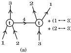
Figure 2: (a) The two-particle correlation piece $h^{\rm(2pc)}$ of Eq. (36). (b) An example of the three-particle correlation contribution $h^{\rm(3pc)}$. In each case the solid lines are nucleons, and $t$ represents a 2-body off-forward scattering matrix. The two diagrams actually represent the first two terms in the Faddeev series.

A few points of this simple perturbative example can be generalized (see also App. B for examples): According to the definition given in Eq. (1), the function $h$ can be obtained from a given diagram for the energy density (effective potential) by successively cutting three intermediate nucleon lines which we denote by 1, 2, and 3. If the cuts are taken in such a way that, among the remaining lines, there is one (we denote it by 4) whose momentum is fixed by momentum conservation, then the four lines 1, 2, 3, 4 constitute the external legs of a two-particle scattering amplitude (matrix elements of an operator $\hat{t}$), which is the off-forward generalization of the function $f$ defined by Eq. (1). In this case, the resulting diagram can be made disconnected by cutting the line 4, i.e., this line must connect two 2-particle irreducible $t$-blocks, as shown in Fig. 2(a). The expression for this process is then obtained by a generalization of Eq. (34), i.e., replacing $\hat{v}\rightarrow\hat{t}$ and $\epsilon_{i}\rightarrow\varepsilon_{i}$, where the $\varepsilon_{i}$’s are the quasiparticle energies:

$$h^{(\rm 2pc)}(\bm{k}_{1},\bm{k}_{2},\bm{k}_{3};\rho)=\sum_{4}\delta_{\bm{k}_{1}+\bm{k}_{2},\bm{k}_{3}+\bm{k}_{4}}$$

$$\hskip 34.1433pt\times P\,\frac{|\langle 12|\,\hat{t}\,|34\rangle_{a}|^{2}}{\varepsilon_{3}+\varepsilon_{4}-\varepsilon_{1}-\varepsilon_{2}}+\left(1\leftrightarrow 3\right)+\left(2\leftrightarrow 3\right).$$ (36)

The energy denominator in this expression comes from the intermediate state where only the particles 1, 2, 3, 4 are “in the air”, and is the same irrespective of whether particle 4 propagates forward or backward in time. Hence, there is no dependence on the Fermi step function $n_{4}$ of particle 4, which is consistent with the 1-particle reducible character of the process, as explained above for the lowest order case. On the other hand, if the cuts in the diagram for the energy density are taken in any other way, the resulting diagram for $h$ is 1-particle irreducible, and the example shown in Fig. 2(b) is a generalization of the lowest order process of Fig. 1(b). We see that actually the process of Fig. 2(a) is the driving term of the Faddeev equation (one particle is exchanged between an interacting pair and the third particle), and Fig. 2(b) appears in the first iteration of the Faddeev equation Bethe (1965); Day (1981); Fritsch et al. (2005).

In order to get a rough estimate of the two-particle correlation piece $h^{\rm(2pc)}$ and its contribution to the inequality given in Eq. (32), we assume that the 2-particle $t$-matrix in Eq. (36) can be represented by an effective contact interaction, i.e., by the in-medium scattering length Fetter and Walecka (2003). In this case, the angular averages of Eq. (16) concern only the energy denominator of Eq. (36), and with the further assumption that the latter can be obtained from the free expression in Eq. (34) by the replacement $M\rightarrow M^{*}$, assuming an average value of the effective mass in the range given in Eq. (30), the angular integrals can be done analytically (see App. C):

$$\int\frac{{\rm d}\Omega_{2}}{4\pi}\,\int\frac{{\rm d}\Omega_{3}}{4\pi}\left(\frac{P}{\varepsilon_{3}+\varepsilon_{4}-\varepsilon_{1}-\varepsilon_{2}}+(1\leftrightarrow 3)+(2\leftrightarrow 3)\right)$$

$$=\frac{M^{*}}{p_{F}^{2}}\,\left(3\ln 2\right)\,,$$ (37)

$$3\,\int\frac{{\rm d}\Omega_{2}}{4\pi}\,\int\frac{{\rm d}\Omega_{3}}{4\pi}\,\left(\bm{\hat{k}}_{1}\cdot\bm{\hat{k}}_{2}\right)$$

$$\hskip 56.9055pt\times\left(\frac{P}{\varepsilon_{3}+\varepsilon_{4}-\varepsilon_{1}-\varepsilon_{2}}+(1\leftrightarrow 3)+(2\leftrightarrow 3)\right)$$

$$=-\frac{M^{*}}{p_{F}^{2}}\,\left(1-\ln 2\right)\,.$$ (38)

Because these simple expressions indicate that $\ell=1$ contributions are suppressed by large factors compared to the $\ell=0$ contributions, we neglect the $\ell=1$ terms in the following. To be specific, we assume that the matrix elements ${}_{a}\langle 34|\,\hat{t}\,|12\rangle$ can be replaced by the $\ell=0$ part of an effective interaction of the Landau-Migdal type Migdal (1967); Migdal et al. (1990); Kamerdzhiev et al. (2004):

$${}_{a}\langle 34|\,\hat{t}\,|12\rangle=f_{0}\,\left(\delta_{31}\cdot\delta_{42}\right)+f_{0}^{\prime}\,\left(\bm{\tau}_{31}\cdot\bm{\tau}_{42}\right)$$

$$\hskip 34.1433pt+g_{0}\,\left(\bm{\sigma}_{31}\cdot\bm{\sigma}_{42}\right)+g_{0}^{\prime}\,\left(\bm{\sigma}_{31}\cdot\bm{\sigma}_{42}\right)\,\left(\bm{\tau}_{31}\cdot\bm{\tau}_{42}\right),$$ (39)

where the notation indicates that the spin and isospin operators are defined to act in the particle-hole channel. As usual, the effect of exchange terms is assumed to be included in the interaction parameters. Performing then the spin-isospin sum over 4 as well as the spin-isospin averages over 1, 2, 3 in Eq. (36), we obtain

$$h_{0}^{\rm(2pc)}=\frac{M^{*}}{p_{F}^{2}}\cdot\left(3\ln 2\right)\cdot\frac{1}{4}\left(f_{0}^{2}+3f_{0}^{{}^{\prime}2}+3g_{0}^{2}+9g_{0}^{{}^{\prime}2}\right)\,.$$ (40)

In terms of the dimensionless interaction parameters of Eqs. (10) and (21), this can be expressed as

$$H_{0}^{\rm(2pc)}=\ln 2\cdot\frac{1}{4}\left(F_{0}^{2}+3F_{0}^{{}^{\prime}2}+3G_{0}^{2}+9G_{0}^{{}^{\prime}2}\right).$$ (41)

In order to estimate the 2pc contributions to the inequality given in Eq. (32), we refer to recent calculations done by using several parameter sets of the extended Skyrme interaction Zhang and Chen (2016) and chiral effective field theory Holt et al. (2018). (Both calculations are consistent with the ranges given in Eq. (27) for the incompressibility and Eq. (30) for the effective mass.) Using the values for the Landau-Migdal parameters given in Table IV of Ref. Zhang and Chen (2016), and in Figs. 9 and 10 of Ref. Holt et al. (2018) at the saturation density, we see that the values for the quantity $\frac{M}{M^{*}}\,H_{0}^{\rm(2pc)}$ are between $0.75$ and $1.23$. Comparison with Eq. (32) then indicates that the 2pc piece alone is too small to reproduce the empirical results. This gives us a hint that the three-particle correlation term in Eq. (33) plays an important role for the skewness of nuclear matter.

V SUMMARY

In this paper we used the framework of the Landau-Migdal theory to express the skewness of nuclear matter in terms of the effective nucleon mass, its slope as a function of momentum, and two-body as well as three-body interaction parameters. Our main result is summarized by the formula given in Eq. (26), where $H_{0}$ and $H_{1}$ are the dimensionless three-body Landau-Migdal parameters, which we defined in Eq. (21) via the $\ell=0$ and $\ell=1$ moments of the three-body forward scattering amplitude $h$. We pointed out that, in order to explain the range of empirical values for $J$ given in Eq. (28), one needs a large positive contribution from the three-body interaction terms, as expressed by Eq. (32). We attempted to make a rough estimate of the contributions of two-nucleon correlations [see Figs. 1(a) and 2(a)] to those three-body parameters, and found that they are of the right sign but very likely too small to explain the empirical values of $J$. We find this to be an important hint that three-particle correlation processes, like those shown in Figs. 1(b) and 2(b), play an important role for the skewness of nuclear matter.

Usually the effect of three-particle interactions are incorporated by using effective density-dependent two-particle interactions. In view of the long and important history of studies on three-particle correlations in nuclear matter, however, it would be interesting to assess our results more quantitatively, by using for example the Faddeev method in the framework of effective field theories.

Appendix A GALILEI INVARIANCE

For completeness we review here the derivation of the Landau relation between $M^{*}$ and $f_{1}$: One considers the variation of the quasiparticle energy which arises from the change of the distribution function due to a Galilei transformation from the rest system of nuclear matter to a system which moves with velocity $\bm{u}\equiv\bm{p}/M$, where $M$ is the free nucleon mass. To first order in $p$ these variations are given by

$$\delta n_{\bm{k}} =-(\bm{\hat{k}}\cdot\bm{p})\,\delta(p_{F}-k)\,,$$ (42)

$$\delta\varepsilon(\bm{k};\rho) =4\int\frac{{\rm d}^{3}k_{2}}{(2\pi)^{3}}\,f(\bm{k},\bm{k}_{2};\rho)\,\delta n_{\bm{k}_{2}}$$

$$=-\frac{2p_{F}^{2}}{3\pi^{2}}\left(\bm{\hat{k}}\cdot\bm{p}\right)\,f_{1}(k,p_{F};\rho)\,.$$ (43)

On the other hand, the quasiparticle energy should transform in the same way as a Hamiltonian in classical mechanics, i.e; $\varepsilon^{\prime}(\bm{k}^{\prime};\rho)=\varepsilon(\bm{k};\rho)-\frac{\bm{k}\cdot\bm{p}}{M}+\frac{p^{2}}{2M}$, where $\bm{k}^{\prime}=\bm{k}-\bm{p}$. From this it follows that $\varepsilon^{\prime}(\bm{k};\rho)=\varepsilon(\bm{k}+\bm{p};\rho)-\frac{\bm{k}\cdot\bm{p}}{M}-\frac{p^{2}}{2M}$, and to first order in $p$,

$$\delta\varepsilon(\bm{k};\rho)=\left(\bm{k}\cdot\bm{p}\right)\left(\frac{1}{M^{*}(k,\rho)}-\frac{1}{M}\right)\,,$$ (44)

where we used the definition given in Eq. (9). The requirement that Eqs. (43) and (44) are identical leads to the desired relation of Eq. (11) in the main text:

$$\frac{k}{M^{*}(k;\rho)}+\frac{2p_{F}^{2}}{3\pi^{2}}f_{1}(k,p_{F};\rho)=\frac{k}{M}\,,$$ (45)

which holds for any values of $k$ and $\rho$. For the case $k=p_{F}$, this becomes the familiar Landau effective mass relation.

As explained in the main text, by taking derivatives of Eqs. (7) and (11) one can derive Eq. (18). Here we show that this relation can also be derived by the requirement of Galilei invariance of the 2-particle forward scattering amplitude: Under the change given by Eq. (42) of the quasiparticle distribution function, the scattering amplitude changes according to

$$\delta f(\bm{k}_{1},\bm{k}_{2};\rho)=-4\int\frac{{\rm d}^{3}k_{3}}{(2\pi)^{3}}$$

$$\hskip 68.2866pt\,h(\bm{k}_{1},\bm{k}_{2},\bm{k}_{3};\rho)\left(\bm{p}\cdot\bm{\hat{k}}_{3}\right)\delta(p_{F}-k_{3})\,.$$ (46)

On the other hand, the Galilei invariance of the scattering amplitude is expressed as $f^{\prime}(\bm{k}^{\prime}_{1},\bm{k}^{\prime}_{2};\rho)=f(\bm{k}_{1},\bm{k}_{2};\rho)$, where $\bm{k}_{i}^{\prime}=\bm{k}_{i}-\bm{p}$. From this it follows, to first order in $p$, that $\delta f(\bm{k}_{1},\bm{k}_{2};\rho)=\bm{p}\cdot\left({\bm{\nabla}}_{k_{1}}+{\bm{\nabla}}_{k_{2}}\right)\,f(\bm{k}_{1},\bm{k}_{2};\rho)$. The requirement that this change is the same as Eq. (46) gives

$$\left({\bm{\nabla}}_{k_{1}}+{\bm{\nabla}}_{k_{2}}\right)\,f(\bm{k}_{1},\bm{k}_{2};\rho)$$

$$\hskip 28.45274pt=-4\int\frac{{\rm d}^{3}k_{3}}{(2\pi)^{3}}\,h(\bm{k}_{1},\bm{k}_{2},\bm{k}_{3};\rho)\,\bm{\hat{k}}_{3}\,\delta(p_{F}-k_{3})\,.$$ (47)

Multiplying this relation by $\bm{\hat{k}}_{1}$ and integrating over the directions of $\bm{k}_{2}$ this becomes

$$\int\frac{{\rm d}\Omega_{2}}{4\pi}\left(\bm{\hat{k}}_{1}\cdot{\bm{\nabla}}_{k_{1}}+\bm{\hat{k}}_{1}\cdot{\bm{\nabla}}_{k_{2}}\right)f(\bm{k}_{1},\bm{k}_{2};\rho)$$

$$=-\frac{2p_{F}^{2}}{\pi^{2}}\int\frac{{\rm d}\Omega_{2}}{4\pi}\int\frac{{\rm d}\Omega_{3}}{4\pi}\left(\bm{\hat{k}}_{1}\cdot\bm{\hat{k}}_{3}\right)h(\bm{k}_{1},\bm{k}_{2},\bm{k}_{3};\rho)|_{k_{3}=p_{F}}\,.$$

We consider this relation for the case $k_{1}=k_{2}=p_{F}$. In the first term on the l.h.s. we simply have $\bm{\hat{k}}_{1}\cdot{\bm{\nabla}}_{k_{1}}=\partial/\partial k_{1}$. For the second term, we can use a partial integration in $\bm{k}_{2}$ to show that

$$\int\frac{{\rm d}\Omega_{2}}{4\pi}\left(\bm{\hat{k}}_{1}\cdot{\bm{\nabla}}_{k_{2}}\right)f(\bm{k}_{1},\bm{k}_{2};\rho)$$

$$=\int\frac{{\rm d}\Omega_{2}}{4\pi}\left(\hat{\bm{k}_{1}}\cdot\hat{\bm{k}_{2}}\right)\left(\frac{2}{p_{F}}+\frac{\partial}{\partial k_{2}}\right)f(\bm{k}_{1},\bm{k}_{2};\rho)$$

$$=\frac{1}{3}\left(\frac{2}{p_{F}}+\frac{\partial}{\partial k_{2}}\right)f_{1}(k_{1},k_{2};\rho).$$

Substituting this for the second term on the l.h.s. of Eq. (LABEL:s), and using the definition given in Eq. (16) as well as the symmetry of $h$ in the momentum variables, leads to Eq. (18).

Appendix B PERTURBATION THEORY

Figure 3: Hugenholtz diagram for the second order contribution to the energy density. The solid lines represent nucleons, and the black circles represent the antisymmetrized nuclear potential.

For illustration of the discussions in Sec. IV, we summarize the familiar expressions for the energy density and the two- and three-particle forward scattering amplitudes in second order perturbation theory Brown (1971); Negele and Orland (1998). The expression for the energy density is

$$E^{(2)} =-\frac{1}{4}\sum_{1234}\,\delta_{\bm{k}_{1}+\bm{k}_{2},\bm{k}_{3}+\bm{k}_{4}}\,\frac{|\langle 12|\hat{v}|34\rangle_{a}|^{2}}{\epsilon_{3}+\epsilon_{4}-\epsilon_{1}-\epsilon_{2}}$$

$$\times n_{1}\,n_{2}\,\left(1-n_{3}\right)\,\left(1-n_{4}\right)\,.$$ (49)

Here we use the schematic notations explained in Sec. IV, and $n_{i}\equiv n_{k_{i}}=\theta(p_{F}-k_{i})$ is the Fermi step function. The corresponding Hugenholtz diagram Negele and Orland (1998) is shown in Fig. 3. The second order contribution to the two-particle forward scattering amplitude obtained from Eq. (49) is given by

$$f^{(2)}(\bm{k}_{1},\bm{k}_{2};\rho)=\frac{\delta^{2}E^{(2)}}{\delta n_{1}\,\delta n_{2}}$$

$$=\frac{1}{2}\sum_{34}\,\delta_{\bm{k}_{1}+\bm{k}_{2},\bm{k}_{3}+\bm{k}_{4}}\,\frac{|\langle 12|\hat{v}|34\rangle_{a}|^{2}}{\epsilon_{3}+\epsilon_{4}-\epsilon_{1}-\epsilon_{2}}\,\left(n_{3}+n_{4}-1\right)$$ (50)

$$+\sum_{34}\,\delta_{\bm{k}_{1}+\bm{k}_{3},\bm{k}_{2}+\bm{k}_{4}}\,\,\frac{|\langle 13|\hat{v}|24\rangle_{a}|^{2}}{\epsilon_{2}+\epsilon_{4}-\epsilon_{1}-\epsilon_{3}}\,\left(n_{3}-n_{4}\right)\,.$$ (51)

The corresponding Hugenholtz diagrams are shown in Fig. 4. The term Eq. (50) is represented by the left diagram, where the bubble graph has two possible time orderings corresponding to two particles or two holes in the intermediate state. The term Eq. (51) is represented by the right diagram, where again the bubble graph has two possible time orderings, corresponding to forward and backward propagating particle-hole intermediate states. An average over the spin and isospin components of particles 1, 2 are implicitly assumed in the above schematic notations.

Figure 4: Hugenholtz diagrams for the two-particle forward scattering amplitude. The left diagram represents Eq. (50), and the right diagram represents Eq. (51). The solid lines represent nucleons, and the black circles represent the nuclear potential.

By relabeling indices, it is easy to verify that

$$f^{(2)}(\bm{k}_{1},\bm{k}_{2};\rho)=f^{(2)}(\bm{k}_{1},\bm{k}_{2};\rho=0)+\sum_{3}\,n_{3}$$

$$\times\left[\sum_{4}\delta_{\bm{k}_{1}+\bm{k}_{2},\bm{k}_{3}+\bm{k}_{4}}\,\frac{|\langle 12|\,\hat{v}\,|34\rangle_{a}|^{2}}{\epsilon_{3}+\epsilon_{4}-\epsilon_{1}-\epsilon_{2}}+\left(2\leftrightarrow 3\right)+\left(1\leftrightarrow 3\right)\right]\,.$$ (52)

From this expression it is clear that the second order contribution to the three-particle forward scattering amplitude:

$$h^{(2)}(\bm{k}_{1},\bm{k}_{2},\bm{k}_{3};\rho)=\frac{\delta f^{(2)}(\bm{k}_{1},\bm{k}_{2};\rho)}{\delta n_{3}},$$

is given by Eq. (34). The only non-trivial point to note is how the principal value emerges. To see this, one has to go back to Eq. (49) and add the infinitesimal $-i\delta$ in the denominator, although this is irrelevant for the energy density and the two-particle scattering amplitude, which are automatically real. Going through the derivation, one finds Eq. (34), but with an additional contribution

$$\sum_{4}\delta_{\bm{k}_{1}+\bm{k}_{2},\bm{k}_{3}+\bm{k}_{4}}\,|\langle 12|\hat{v}|34\rangle_{a}|^{2}\,i\pi\delta\left(\epsilon_{3}+\epsilon_{4}-\epsilon_{1}-\epsilon_{2}\right)(1-2n_{4})$$

$$+\left(2\leftrightarrow 3\right)+\left(1\leftrightarrow 3\right)\,.$$ (53)

Because $k_{i}=p_{F}$ for $i=1,2,3$, the energy conserving delta function in Eq. (53) requires that also $k_{4}=p_{F}$. In order to avoid such an unphysical imaginary part, one therefore has to define the step function $\theta(x)$ so that $\theta(x=0)=\frac{1}{2}$, which is also suggested by the finite temperature form of $n_{4}$, taking the limit $\epsilon_{4}\rightarrow\epsilon_{F}$ before the limit $T\rightarrow 0$.

We note that Eq. (52), which reads symbolically as $f(1,2)=f_{\rm vac}(1,2)+\sum_{3}h(1,2,3)\,n_{3}$, does not hold in the general case, only its differential form is general. This indicates that some care should be taken in a direct comparison of magnitudes of the dimensionless two-body [Eq. (10)] and three-body [Eq. (21)] parameters.

The discussions given above may be extended to higher orders in perturbation theory, and we just give the relevant Hugenholtz diagrams for the energy density in third and fourth order in Fig. 5 Hammer and Furnstahl (2000); Steele (2000); Bogner et al. (2010). One may use those figures to follow the line of arguments in Sec. IV, leading from the second order result, Eq. (34), to its extension given by Eq. (36).

Figure 5: Top panel: Hugenholtz diagram for the third order contribution to the energy density. Bottom panel: Hugenholtz diagram for the fourth order contribution to the energy density. In both cases the solid lines represent nucleons, and the black circles represent the antisymmetrized nuclear potential.

Appendix C ANGULAR INTEGRALS

If we chose a coordinate system where $\bm{k}_{1}$ points along the $z$ axis, the energy denominator of the first term in Eq. (37) can be expressed as

$$\frac{1}{\epsilon_{3}+\epsilon_{4}-\epsilon_{1}-\epsilon_{2}}\equiv\frac{1}{\epsilon_{\bm{k}_{3}}+\epsilon_{\bm{k}_{1}+\bm{k}_{2}-\bm{k}_{3}}-\epsilon_{\bm{k}_{1}}-\epsilon_{\bm{k}_{2}}}$$

$$\hskip 14.22636pt=\frac{M}{p_{F}^{2}}\frac{1}{(1+z_{2})(1-z_{3})-\sqrt{(1-z_{2}^{2})(1-z_{3}^{2})}\,\cos\phi}\,.$$ (54)

Here $z_{2},\,z_{3}$ are the polar angles of $\bm{k}_{2},\bm{k}_{3}$, and $\phi$ is the relative azimuthal angle between $\bm{k}_{2}$ and $\bm{k}_{3}$. The principal value integration over $\phi$ can be performed by using the formula

$$P\,\int_{0}^{2\pi}\frac{{\rm d}\phi}{a+b\cos\phi}=\frac{2\pi}{\sqrt{a^{2}-b^{2}}}\,\theta(a^{2}-b^{2}),$$ (55)

where $a>0$. This gives

$$\int\frac{{\rm d}\Omega_{2}}{4\pi}\,\int\frac{{\rm d}\Omega_{3}}{4\pi}\,P\,\frac{1}{\epsilon_{3}+\epsilon_{4}-\epsilon_{1}-\epsilon_{2}} =\frac{M}{p_{F}^{2}}\,\frac{\sqrt{2}}{8}\,I_{0}\,,$$ (56)

$$\int\frac{{\rm d}\Omega_{2}}{4\pi}\,\int\frac{{\rm d}\Omega_{3}}{4\pi}\,P\,\frac{\bm{\hat{k}}_{1}\cdot\bm{\hat{k}}_{2}}{\epsilon_{3}+\epsilon_{4}-\epsilon_{1}-\epsilon_{2}} =\frac{M}{p_{F}^{2}}\,\frac{\sqrt{2}}{8}\,I_{1}\,,$$ (57)

where the integrals $I_{0}$ and $I_{1}$ over the polar angles are evaluated as

$$I_{0} =\int_{-1}^{1}{\rm d}z_{2}\,\int_{-1}^{z_{2}}{\rm d}z_{3}\,\frac{1}{\sqrt{(1+z_{2})(1-z_{3})(z_{2}-z_{3})}}$$

$$=4\sqrt{2}\,\ln 2\,,$$ (58)

$$I_{1} =\int_{-1}^{1}z_{2}\,{\rm d}z_{2}\,\int_{-1}^{z_{2}}{\rm d}z_{3}\,\frac{1}{\sqrt{(1+z_{2})(1-z_{3})(z_{2}-z_{3})}}$$

$$=\frac{4}{3}\sqrt{2}\,(1-\ln 2)\,.$$ (59)

The remaining two terms in Eq. (37) can be obtained from the above integrals by a redefinition of integration variables, and the results are

$$\int\frac{{\rm d}\Omega_{2}}{4\pi}\,\int\frac{{\rm d}\Omega_{3}}{4\pi}\left(\frac{P}{\epsilon_{3}+\epsilon_{4}-\epsilon_{1}-\epsilon_{2}}+(1\leftrightarrow 3)+(2\leftrightarrow 3)\right)$$

$$=\frac{M}{p_{F}^{2}}\frac{3\sqrt{2}}{8}I_{0}\,,$$ (60)

$$3\,\int\frac{{\rm d}\Omega_{2}}{4\pi}\,\int\frac{{\rm d}\Omega_{3}}{4\pi}\,\left(\bm{\hat{k}}_{1}\cdot\bm{\hat{k}}_{2}\right)$$

$$\hskip 56.9055pt\times\left(\frac{P}{\epsilon_{3}+\epsilon_{4}-\epsilon_{1}-\epsilon_{2}}+(1\leftrightarrow 3)+(2\leftrightarrow 3)\right)$$

$$=-\frac{M}{p_{F}^{2}}\frac{3\sqrt{2}}{8}I_{1}\,,$$ (61)

which gives Eqs. (37) and (38) of the main text.

References

- Blaizot (1980) J. P. Blaizot, Phys. Rept. 64, 171 (1980).
- Mahaux et al. (1985) C. Mahaux, P. F. Bortignon, R. A. Broglia and C. H. Dasso, Phys. Rept. 120, 1 (1985).
- Danielewicz et al. (2002) P. Danielewicz, R. Lacey and W. G. Lynch, Science 298, 1592 (2002) [arXiv:0208016 [nucl-th]].
- Bethe (1990) H. A. Bethe, Rev. Mod. Phys. 62, 801 (1990).
- Lattimer (2012) J. M. Lattimer, Ann. Rev. Nucl. Part. Sci. 62, 485 (2012) [arXiv:1305.3510 [nucl-th]].
- Baym et al. (2018) G. Baym, T. Hatsuda, T. Kojo, P. D. Powell, Y. Song and T. Takatsuka, Rept. Prog. Phys. 81, 056902 (2018) [arXiv:1707.04966 [astro-ph.HE]].
- Li et al. (2018) B.-A. Li, B.-J. Cai, L.-W. Chen and J. Xu, Prog. Part. Nucl. Phys. 99, 29 (2018) [arXiv:1801.01213 [nucl-th]].
- Piekarewicz (2010) J. Piekarewicz, J. Phys. G37, 064038 (2010) [arXiv:0912.5103 [nucl-th]].
- Zhang and Chen (2013) Z. Zhang and L.-W. Chen, Phys. Lett. B726, 234 (2013) [arXiv:1302.5327 [nucl-th]].
- Cai and Chen (2017) B.-J. Cai and L.-W. Chen, Nucl. Sci. Tech. 28, 185 (2017) [arXiv:1402.4242 [nucl-th]].
- Bethe et al. (1963) H. A. Bethe, B. H. Brandow and A. G. Petschek, Phys. Rev. 129, 225 (1963).
- Rajaraman (1963) R. Rajaraman, Phys. Rev. 129, 265 (1963).
- Brown (1971) G. E. Brown, Rev. Mod. Phys. 43, 1 (1971).
- Serot and Walecka (1986) B. D. Serot and J. D. Walecka, Adv. Nucl. Phys. 16, 1 (1986).
- Müller and Serot (1995) H. Müller and B. D. Serot, Phys. Rev. C52, 2072 (1995) [arXiv:nucl-th/9505013 [nucl-th]].
- Meng et al. (2016) J. Meng, P. Ring and P. Zhao, Int. Rev. Nucl. Phys. 10, 21 (2016).
- Zhang and Chen (2016) Z. Zhang and L.-W. Chen, Phys. Rev. C 94, 064326 (2016).
- Speth et al. (2014) J. Speth, S. Krewald, F. Grümmer, P. G. Reinhard, N. Lyutorovich and V. Tselyaev, Nucl. Phys. A928, 17 (2014) [arXiv:1402.3249 [nucl-th]].
- Kaplan et al. (1998) D. B. Kaplan, M. J. Savage and M. B. Wise, Nucl. Phys. B534, 329 (1998) [arXiv:9802075 [nucl-th]].
- Hammer and Furnstahl (2000) H. W. Hammer and R. J. Furnstahl, Nucl. Phys. A678, 277 (2000) [arXiv:0004043 [nucl-th]].
- Steele (2000) J. V. Steele, arXiv:0010066 [nucl-th].
- Bogner et al. (2010) S. K. Bogner, R. J. Furnstahl and A. Schwenk, Prog. Part. Nucl. Phys. 65, 94 (2010) [arXiv:0912.3688 [nucl-th]].
- Holt et al. (2018) J. W. Holt, N. Kaiser and T. R. Whitehead, Phys. Rev. C97, 054325 (2018) [arXiv:1712.05013 [nucl-th]].
- Pearson (1991) J. M. Pearson, Phys. Lett. B271, 12 (1991).
- Kouno et al. (1995) H. Kouno, K. Koide, T. Mitsumori, N. Noda, A. Hasegawa and M. Nakano, Phys. Rev. C52, 135 (1995).
- Frohlich et al. (1998) N. Frohlich, H. Baier and W. Bentz, Phys. Rev. C57, 3447 (1998).
- Steiner et al. (2010) A. W. Steiner, J. M. Lattimer and E. F. Brown, Astrophys. J. 722, 33 (2010) [arXiv:1005.0811 [astro-ph.HE]].
- Migdal (1967) A. B. Migdal, Theory of finite Fermi systems and applications to atomic nuclei (New York, Wiley, 1967) p. 319.
- Migdal et al. (1990) A. B. Migdal, E. E. Saperstein, M. A. Troitsky and D. N. Voskresensky, Phys. Rept. 192, 179 (1990).
- Kamerdzhiev et al. (2004) S. Kamerdzhiev, J. Speth and G. Tertychny, Phys. Rept. 393, 1 (2004) [arXiv:nucl-th/0311058 [nucl-th]].
- Landau (1956) L. D. Landau, Sov. Phys. JETP 3, 920 (1956).
- Landau (1957) L. D. Landau, Sov. Phys. JETP 5, 101 (1957).
- Landau (1959) L. D. Landau, Sov. Phys. JETP 8, 70 (1959).
- Baym and Pethick (2004) G. Baym and C. Pethick, Landau Fermi-Liquid Theory: Concepts and Applications (WILEY-VCH Verlag, 2004).
- Baym and Chin (1976) G. Baym and S. A. Chin, Nucl. Phys. A262, 527 (1976).
- Nozières (1964) P. Nozières, Theory of interacting Fermi systems (W.A. Benjamin, New York, 1964).
- Negele and Orland (1998) J. Negele and H. Orland, Quantum Many-particle Systems (Westview Press, 1998).
- Ring and Schuck (1980) P. Ring and P. Schuck, The nuclear many-body problem (Springer-Verlag, New York, 1980).
- Chen et al. (2009) L.-W. Chen, B.-J. Cai, C. M. Ko, B.-A. Li, C. Shen and J. Xu, Phys. Rev. C80, 014322 (2009) [arXiv:0905.4323 [nucl-th]].
- Bethe (1965) H. A. Bethe, Phys. Rev. 138, B804 (1965).
- Day (1981) B. D. Day, Phys. Rev. C24, 1203 (1981).
- Fritsch et al. (2005) S. Fritsch, N. Kaiser and W. Weise, Nucl. Phys. A750, 259 (2005) [arXiv:nucl-th/0406038 [nucl-th]].
- Hugenholtz and van Hove (1958) N. M. Hugenholtz and L. van Hove, Physica 24, 363 (1958).
- Blaizot and Friman (1981) J. P. Blaizot and B. L. Friman, Nucl. Phys. A372, 69 (1981).
- van Dalen et al. (2005) E. N. E. van Dalen, C. Fuchs and A. Faessler, Phys. Rev. C72, 065803 (2005) [arXiv:nucl-th/0511040 [nucl-th]].
- Fetter and Walecka (2003) A. L. Fetter and J. D. Walecka, Quantum Theory of Many-Particle Systems (Dover Publications, 2003).