ES2019-001

Reframing Threat Detection: Inside esINSIDER

1 Introduction

Organizations are spending millions of dollars a year on computer and network security products, yet we continue to see growing numbers of large-scale compromises by persistent threats and insider threats. When an industry throws more resources at a problem, but the situation continues to worsen, it behooves us to step back and understand what is missing. Ignoring this new risk used to be a rational business decision because only governments and large corporations needed to worry about being targeted by persistent threats and insider threats. Today, they are tangible risks for practically every business.

Current security approaches struggle to detect ongoing threat campaigns because 1) they focus on individual events and alerts, 2) they tend to overemphasize preventing (or detecting) initial access and misuse, and 3) significant data storage, processing, and analytics are required to aggregate and correlate events over weeks. When security analysts review individual alerts, they are reviewing isolated information tidbits; it is exceedingly hard to see if they fit into a larger story of a serious threat. As a result, serious threats are lost in the stream of false positives and low priority problems [35]. The intense focus on stopping initial access is problematic because the threat actor only needs to succeed once, and they get an unlimited number of tries. A well-resourced threat actor will eventually get in; if defenders ignore internal network patterns, the threat actor can operate inside the network—the bulk of their campaign—with impunity. In our experience, only a minority of organizations watch for suspicious internal network actions, and virtually nobody connects events and alerts together over weeks to detect an ongoing campaign. As a result, network defenders lack the information to form a clear picture of the long-term threats unfolding in their networks.

To better defend against persistent and insider threats, defenders need to start thinking like a threat actor to understand what they must do to complete their campaign. The threat actor, whether an external actor or a malicious insider, has a goal of identifying, collecting, and stealing data of value to their mission. The specific techniques used to gain initial access and to maintain a persistent foothold within a network change based upon a number of variables. Hunting for evidence of tools and tactics that change so frequently is doomed to be a game of catch up (e.g., [9]). In contrast, the adversary campaign behaviors inside a compromised organization, abstracted from the specifics of the techniques used, remain consistent across campaigns and across a wide range of threat actors. We can reduce the detection challenge by focusing on the required meta-goals of the threat actor and how they differ from data flows and movements in legitimate business operations. Regardless of the actor’s specific choices—how to move laterally, which exploit to throw, which credential to use, etc.—the majority of their campaign focuses on identifying, collecting, and extracting as much information of value (to the threat actor) from the target organization as possible. These campaign behaviors—internal reconnaissance, collection, and exfiltration—are required and occur repeatedly, creating multiple opportunities for the threat actor to be detected.

In this paper we describe esINSIDER, an automated tool that detects potential adversary campaigns. esINSIDER aggregates clues from log data, over extended time periods, and proposes a small number of ThreatCase^® results for human experts to review. The core ideas are to 1) detect fundamental campaign behaviors by following data movements over extended time periods, 2) link together behaviors associated with different meta-goals, and 3) use machine learning to understand what activities are expected and consistent for each individual network. We call this approach campaign analytics because it focuses on the threat actor’s campaign goals and the intrinsic steps to achieve them. Cases package together related information so the analyst can see a bigger picture of what is happening, and their evidence includes internal network activity resembling reconnaissance and data collection. Linking different campaign behaviors (internal reconnaissance, collection, exfiltration) reduces false positives from business-as-usual activities and creates opportunities to detect threats before a large exfiltration occurs. Machine learning makes it practical to deploy this approach by reducing the amount of tuning needed.

It is important to understand how this approach fits into a complete cybersecurity portfolio. We can organize cybersecurity into four broad strategies: 1) prevention, 2) rapid intrusion detection and response, 3) threat hunting, and 4) proactive closing of gaps (not discussed in this paper).

Prevention is all about preventing problems from starting, and it includes all the best practices learned over decades: end-point defenses, strong passwords, appropriately configured firewalls, least privilege, two factor authentication, user training, reducing the organization’s threat surface, segmented networks, etc. Organizations obviously should invest in prevention: it stops many problems before they become problems. At the same time, prevention will never be 100% effective because network defenders cannot achieve perfection. The threat actor only needs to find one gap, only needs to find one user who clicks on a phishing link, only needs to get lucky once.

Rapid intrusion detection and response acknowledges prevention will sometimes fail and then tries to detect intrusions after they have started. It includes network intrusion detection (e.g., Snort, Bro), endpoint detection, and log analysis. Naturally, one wants to detect intrusions as fast as possible, before a small problem becomes a large problem. Intrusion detection raises the bar and improves a network’s security, but the game is still asymmetric. A sophisticated threat actor with enough time and resources will find a way to avoid intrusion detection systems.

Threat hunting proactively searches for undetected threats that are already in the network and have avoided detection by front line security tools. esINSIDER is an automated tool to assist with the discovery of these threats. Unlike user entity behavior analysis (UEBA), esINSIDER uses campaign analytics. This perspective is a paradigm shift in detecting persistent and insider threats:

• These campaign steps are almost always required for the campaign to succeed. Skipping a step, to avoid detection, makes it harder for the threat actor to complete the mission.

• Campaign detection can focus on many fewer activities: just the ones that would directly execute campaign steps. In a nutshell, we need to follow the data. It almost does not matter if the threat actor invents a new technique; they still need to find, access, and attempt to exfiltrate the data.

• It inverts the asymmetry. The threat actor needs to execute their whole campaign. Defenders only need to identify enough of a subset of the campaign to catch them.

As a result, defenders can have the advantage and stop playing catch up.

All of these approaches contribute to the same end goal: protect the organization’s digital and physical assets. They are also complementary. E.g., discoveries from campaign analytics can improve prevention and rapid intrustion detection & response. You should use all of them, and they are all on-going, parallel programs.

The rest of the paper is organized as follows. First, we present a hypothetical interview with a sophisticated threat actor to help explain the threat actor’s perspective and how they operate (Section 2). Next, we describe the fundamental requirements for effective detection of sophisticated threat actors (Section 3). Section 4 explains the basic design of esINSIDER, and Section 5 concludes. For information about the automated machine learning used in esINSIDER, see Appendix A.

2 Hypothetical Interview with an Operator

The Operator has executed campaigns for state actors and various other entities. She has been a member of and managed the teams responsible for executing these campaigns, in addition to directing other teams of engineers and developers responsible for the tools and infrastructure required to execute threat actor campaigns. She is also experienced with operations based on human access, i.e. insider threat.

• There is a ton of activity in the security industry. E.g., every year, thousands of CVEs are disclosed, and millions of new malware are found. It seems like you need to move fast in security to keep up with the latest developments. How much does this constant flurry of activity disrupt your operations?

• This may be surprising, but not very much, which is good news for me and my teams. The focus on initial access, signatures, etc. misses the majority of where I spend my time, focus, and energy during operations. The perimeter is important, and high walls with barbed wire on them is something that I have to defeat. But I really only have to defeat it once, and I get, essentially, an unlimited number of attempts to do so. By focusing on signatures and CVEs, the defender is overlooking the majority of where I spend my time and effort. They essentially overlook my campaign.

• Can you clarify what you mean by “campaign”?

• The campaign is maintaining covert and/or clandestine access to a targeted network and repeatedly finding information of value over time. This isn’t a singular act or one-time event; instead, I, or my team, spend time finding, collecting, exfiltrating, evaluating the exfiltrated data, and then possibly modifying or re-tasking the mission based on what was learned from the information we obtained.

• Can you give an example?

• Think about the OPM “hack”, the large healthcare and medical compromises, the “Panama Papers”, or even how an insider may identify, collect, and abscond with sensitive documents when they leave to go work for a competitor. Everyone talks about what was lost and the way I got in, but nobody talks about the main effort of my job which is what I was doing for days, months, sometimes years, while I’m inside.

  The initial access is just the first of many steps, several of which can happen simultaneously. I’m looking for things like running services and open ports, in order to figure out what kind of hardware and software is deployed on the network (since this then largely dictates the types of tools and tradecraft I will use). This internal network reconnaissance helps illuminate the network for me. In particular, I want to know where the different repositories of data are and how this target information is accessed within the environment. It’s all about the data that I’m looking for. Once I start to locate and collect data that I want to get out, I need to move that data from wherever I found it to somewhere from which I can safely exfiltrate it. Because look, I’d love to simply throw the data from where it lives internally to my server externally, but Murphy is always around. Inevitably, I can’t just exfiltrate it from where I found it—or at least not without drawing a big bullseye on myself. So now I’m moving sometimes small, sometimes large volumes of data around the network at a particular point in time. However, over the duration of my operation this is almost always a large amount of data. And finally, I’ll exfiltrate this data out to a system I control. The key, though, is that this isn’t a serial process, or a process that occurs only once. It happens multiple times, sometimes in various orders, and because nobody is looking for me doing this, I do it for as long as I can, which sometimes goes on for years.

• OK, what does a campaign look like from your perspective?

• There can be a lot of complexity in it, to be honest. From start to finish, there is sometimes enormous technical and tradecraft issues to be discussed and decided. Networks are so dynamic day over day that my own tool and tradecraft choices aren’t even remotely static, which works to my advantage if defenders are just looking for a particular tool’s signature.

  But looking at everything I and/or my team does, you can really bucket it all into some key areas. First, let’s ignore the initial intrusion because—let’s be honest—eventually I get in.

  So, once I’m in, the first thing to consider is internal network reconnaissance [stage 3]. As I said before, this is where we’re discovering things about the network in order to figure out where the different repositories of data are and how we will need to access them.

  As we start to find data that we want to get out, we start moving it around so that we can eventually get it out. This internal data movement [stage 4] is where I am probably the most exposed but also the least concerned, since no one really watches the east-west data flow very closely. Also, at this point, I’m using legitimate credentials that I’ve obtained to get the data. If the defenders looked for one of their own systems hoovering up information from a range of internal servers, rather than trying to figure out when or how I stole Joe-the-admin’s credentials, I’d have a really hard time.

  At some point I’ll start exfiltrating data [stage 5], both the “operational intelligence” sort of data (low volumes, but things like screenshots, keylogs, etc.), and the big fish collections like the massive, sensitive database dumps. This is where some people are starting to look, since it’s at the perimeter. But most of the time companies are blacklisting the exfil destinations that I used in the past—not the new ones I’m using.

  All of this data comes out and enters into an analytics and evaluations stage [stage 6], where I, my team, or others evaluate it, make some decisions, and sort of re-task or redirect based on what we’ve found and learned.

  That’s what my life is, and you will notice that I didn’t talk at all about my tools or exploits, because I can change them up easily.

• Why don’t the networks and companies see you doing this reconnaissance, collection, and exfiltration?

• First, they aren’t looking. Everyone is very focused on the perimeter. But it’s not where the treasure is for me. The treasure is on the inside; the treasure is the data inside the target. That’s where I’m focused, not the perimeter other than initially and for minor things here and there. Once I’ve established persistent clandestine access to the network, I’m easily traversing the perimeter, in both directions as needed.

  Second, when they do look, my victims aren’t thinking like an operator running a campaign. They’re looking for point-in-time alerts, or a proverbial needle in a haystack. They’re not looking across various data sources, they’re not linking these things together to see what kind of campaign narrative comes out of it.

• OK, let’s go through these different activities inside your targets in a bit more detail. Walk me through your day to day after you’re already inside your target, from the perspective of the operator. Talk about the initial, and any ongoing, reconnaissance activities.

• I’m spending a significant amount of time doing reconnaissance [stage 3]. There’s a lot for me to discover and figure out about this network: the hardware, the software, the users, the security posture, etc. All of this is in support of my goal, which is to find the large repositories of data that I want. I’m sort of always looking over my shoulder and both ways before I cross the proverbial street. Luckily most modern enterprise networks are super noisy, allowing me to be relatively blatant in how I look around and discover stuff.

• You said “blatant”, but the industry talks about sophisticated threat actors using low-and-slow attacks. How often are you doing this? Could it be easily detected?

• Well that’s the thing, I get to conduct this sort of behavior based on how I perceive the threat environment. Sometimes I need to go low and slow, other times I can be a bit more blatant. I don’t need to do active reconnaissance too frequently, I just need to get a good map to work with that is relevant to finding, getting, and exfiltrating the various data stores. I’m looking for all sorts of things; probably 75% of what I discover isn’t necessarily of interest to me specifically, but the data goes back for others to look at and evaluate. Sort of over everything is that there’s a cost associated with what I do and how I do it. For example, walking up and down a /24 with a noisy scan is quick and effective, but leaves more of a “signature” than if I scanned just small clusters of workstations across a few days or a few weeks—or more. Same deal with individual hosts: I can learn a lot at the network level, but often I need to get a bit deeper on the individual hosts to gain a better understanding of the what and the how. But there’s an obvious risk to this. This is what most network defenders tend to forget: every decision I make is a trade-off that has been considered and decided, before I ever hit the enter key.

• You’ve done or are doing this reconnaissance, and I presume that you start to identify where the data lives and what types of protocols and credentials access it. What happens then?

• This is the collection/staging [stage 4], that I mentioned before. And to be clear, as I just talked about for reconnaissance: every decision I make about how I execute my op has some type of cost associated to me. So, let’s say I find the database with the data that I care about, and it’s 50GBs of data. The database is internal only, so I have to take that data and put it onto a host that has Internet access. Moving 50GBs around the network might seem blatant, but people are almost never looking at this east-west flow from internal system to internal system. As a result, I can generally move my data around inside the network with relative ease. It gets a bit more complicated in networks that are segmented and have internal controls like firewalls and enclaves and other such things, but these harder target environments are actually exceedingly rare.

  By this time, my risk profile is considerably lower. I can start to mimic legitimate users, for example. This may not seem important, but it means that I often don’t have to exploit and/or even implant machines inside the network. I can use legitimate creds and/or legitimate access paths to interact with internal resources and extract the data that I care about. What this means from a practical standpoint is that all those end-point security tools and such that are looking for malware/implants and all sorts of bad stuff on the inside—I blow right past those.

• So where does that leave the defenders?

• Well, at this point in my campaign I’m pretty well entrenched. I likely understand your network and security posture at least as well as you [the defenders] do. I’ve probably captured a bunch of legitimate creds, I might even be logged into your security interface watching you create and respond to tickets. But even with legitimate credentials that work, it’s not as if the behavior itself is legitimate. Do Claude’s credentials get me access to the database? Sure do! Do I want to ensure I only access the database with Claude’s credentials when Claude is in the office and at his computer? Well, maybe …but that’s a cost to me that I have to consider depending on the operation. So, whatever workstation I am using as my base of operations, from which I will interact with the database (using Claude’s creds), has a behavioral aspect to it that is almost certainly anomalous compared to how data is accessed and moved around the company in support of legitimate business. And that’s the real kicker: creds or no creds, day or night, or whatever other environmental variable is at play: it’s how, when, which direction, and at what volume, and the frequency I interact with the data in the environment that is important—and how that looks and compares to legitimate data accesses, flows, and uses.

• Ok so you’ve done the recon, you’ve found and moved and staged the data; what’s next? I assume you get the data out?

• Of course, [stage 5] exfiltration is key. I have to get the information out before we perform the in-depth analysis on it.

• Why don’t you pre-filter and only take out the things you need? That would reduce the amount you have to exfiltrate, no?

• Actually, there are several reasons why I generally won’t pre-filter the data in the compromised environment. First, maybe there’s good information in the volumes of data that I’ve identified that someone on the back end will find valuable and that I don’t know is interesting ahead of time. I don’t want to leave data on the table; it’s opportunistic. Second, if my scripts and tools are compromised—which happens from time to time—I don’t want the victim to know what I was looking for. If I give that away it can point back to me or my teams, which I don’t want. Not giving away what I find most valuable in their data prevents the organizations from isolating that type of information and making it more difficult for me to get in the future.

• Are you exfiltrating information constantly?

• For the larger throws, it’s not always a constant stream of data, but it isn’t a one-time thing either. I’m usually exfiltrating some pretty decent chunks of data aperiodically over the course of the compromise. Things like screenshots of workstations and keylogs are going to come out relatively frequently if I’m trying to watch and identify a particular person, although these are at a pretty low volume. I see people try to identify the C2 channels or these other small keylogger throws but the defenders are buried in false positives when they look for such small amounts of data. Things like massive database dumps generally come out at higher volume but with less frequency. This is where network defenders could figure out what I’m doing, but the current focus is misplaced, in my opinion. There is a lot of reliance on discovering known bad IPs/domains and then blacklisting them. And everyone celebrates when they discover that a particular IP is a C2 server for some implant in some network. But that external infrastructure, that I control, is incredibly fluid. Not only do I setup new malicious infrastructure to use, but I can also do clever things like take over a legitimate site and use it maliciously, or create fake but real looking domains. Or, use legitimate services like cloud or social media. Bottom line is that I can get around basically all the things you use to try to stop me from getting data in and out. What’s far more relevant is the nature of the behavior itself: what does the internal to external data flow look like, at what volume and what day/time, and how does that compare to how that host—and all other internal hosts—talk to various external sites.

• Now that you’ve exfiltrated the data out, what happens?

• Well that’s the consumption and processing of the data [stage 6], the part that no one on the operations team wants to talk about because it’s not so glamorous, but the analysts love it. Sure, I exfiltrate all this data. But now someone needs to go through that data and derive meaning from it. And from my perspective, some of that meaning is critical because the information gleaned from the exfiltrated data will be used to create additional requirements for me, to do new things or keep doing the same things or to stop doing something.

• Are you always active in a target?

• No, not at all. There’s dozens of factors that dictate how often I’m active inside a target network. Some of them are sexy and interesting, like, in the somewhat uncommon case where the network’s security team is good so I want to minimize my chances of getting caught. Some of them are not so sexy, like, my team is mostly out sick this week, which means no one to catch beacons and no one to pull data. Or that I’m running a lot of operations simultaneously, and I can only light up a few at a time to give them the appropriate attention and care they need. It’s also incredibly variable day over day, week over week. There is rarely as much pattern or automation as people imagine. This is important because a lot of network defenders use time and patterns to try to discover malicious behavior.

  I have to balance my risk of being detected against doing my job. Every time I’m interactive on the network there’s the chance that Murphy will pop up and something will go wrong and I risk being discovered, so I do what I need to do and then stop.

• What do you worry about? What could your targets do that would make your job more difficult?

• Look at each of the stages from my perspective, identify activities that fit my work in each, and then connect across those stages. Understand how I do what I do, abstract the specifics away from the detection—like signatures and tools and exploits and known bad infrastructure—and instead focus on the behaviors within the network.

3 Fundamental Requirements

We believe this difficult problem—detecting threat actors inside a network—is solvable. There are four fundamental requirements to achieve effective detection with a reasonable, practical amount of resources:

1. Focus on the threat actor campaign goals—not tools or artifacts of a single aspect (e.g., do not focus on zero day exploits, specific failed logins, etc.).

2. Automation, machine learning, and interpretability.

3. Adapt to an ever-changing environment.

4. Hard for threat actor to avoid.

Any approach that lacks these necessary pieces will not scale to large networks or will lag behind evolving threat actors.

3.1 Focus on Threat Actor Campaign and Data Movement

Focusing on the threat actor campaign, in a holistic way, is essential to finding the threats that matter. This is a monumental shift in focus away from identifying and alerting on discrete anomalies. Instead, the solution must synthesize and make sense of activity across the campaign lifecycle.

This is important because behaviors are most meaningful in the context of the larger campaign. For example, if a computer:

• maps all the IP addresses in an environment,

• or downloads 250 MB from an internal server it never communicated with before,

• or uploads 15 MB to an external file server,

that could be mildly interesting. Realistically, there is a high chance each of these anomalies, individually, is benign. But if the same computer performed all three activities, that is much more interesting. It is especially interesting if this is not consistent with the computer’s historical activity. The facts start to point more towards threat actor goals than legitimate business functions: it is unlikely that all three anomalies co-occur for the same computer by random chance.

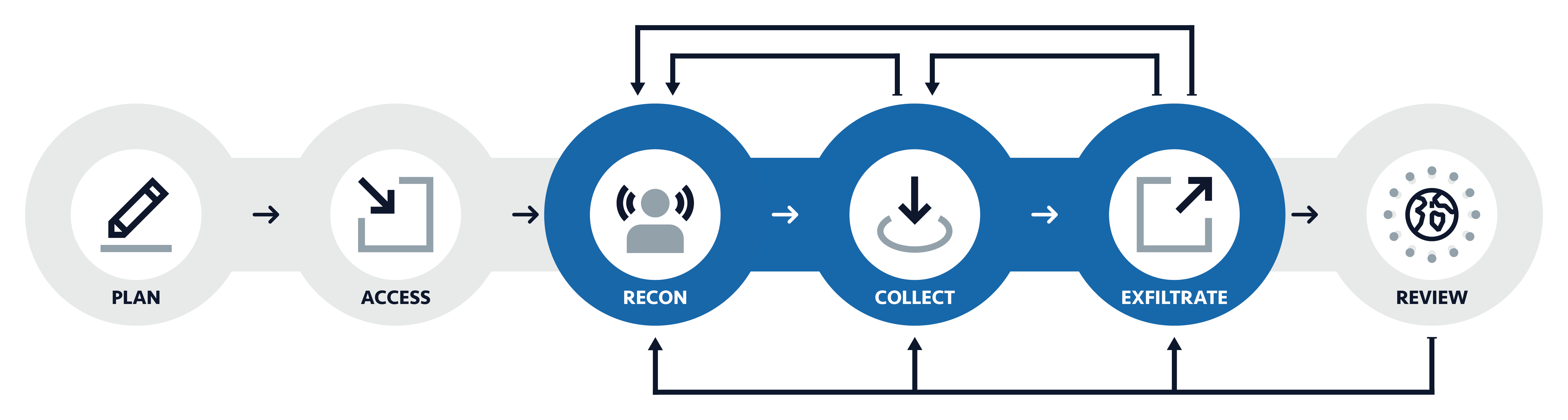
Figure 1: Campaign lifecycle for significant compromises. The blue stages occur inside the target network and therefore can be observed by network defenders. Recon, collection, and exfiltration will repeat during a long campaign, as the campaign proceeds through multiple cycles. Note also that the order of the stages is not fixed. E.g., after exfiltration, the threat actor may collect more data due to information learned in stage 6 (review). See text for more details.

Using a campaign-oriented framework for detection also simplifies what needs to be monitored. You only monitor for behaviors the threat actor must perform, the ones they cannot avoid, to succeed in their mission. Non-essential behaviors (e.g., beaconing) can be changed by a committed threat actor—often at little or no cost—while core behaviors cannot be easily changed. Further, non-essential behaviors are often a source of false positives.

There are several stages in adversary campaigns [44]:

Stage 1: Planning

The threat actor campaign starts with up front planning to figure out how to get access and the initial targeting. This occurs outside the network, involving both public and private sources, and many of the tactics never need to touch the target network itself. As a result, defenders usually cannot detect this activity.

Stage 2: Initial Access

Next, the threat actor gains initial access on the target network using any of a broad arsenal of tools (e.g., phishing, exploiting unpatched software on Internet facing infrastructure, zero day exploits, etc.).

Perhaps surprisingly, monitoring for initial access helps very little with finding an active campaign in the network. The set of tools is highly variable (with threat actors constantly finding new ways in), and typically threat actors remove evidence of the initial access. Failed attempts potentially can be seen by defenders in logs, but this information is not really actionable for detecting if a threat actor later succeeded.

Stage 3: Reconnaissance

After penetrating the network, the malicious actor works to improve their understanding of the network: typical hardware and software configurations, locating key data stores, what endpoint protection is deployed, etc. Reconaissance activities include enumerating and scanning computers on the network, finding new treasure-troves of data, going through local logs, and identifying high-value targets. Legitimate users and systems do not exhibit the same type of uninformed searching and learning the environment.

Stage 4: Collection and Staging

During collection and staging, the threat actor gets access to the data and prepares to exfiltrate it. Sometimes the data can be exfiltrated directly from the computer storing it, but other times it is collected and staged on a different machine. There are many reasons why a threat actor might move the data before exfiltrating it, including:

• Move it to a machine that is always on so that the data can be exfiltrated at chosen times (when defenders are less likely to notice).

• Avoid drawing attention on a computer that administrators or users watch.

• Avoid any risk of crashing an essential server.

The volume and/or breadth of these data movements usually stands out as atypical compared to data accesses triggered by business activities.

Stage 5: Data Exfiltration

Finally, the captured data is moved out of the network to infrastructure the threat actor controls. The particular exfiltration method(s) used are largely determined by the services and pathways permitted on the target network and by the organization’s overall security posture. Regardless of the method, the large-scale, aperiodic movement of data to an external network is a measureable activity that can be detected.

Stage 6: Review

After a threat actor exfiltrates data from a network, their next steps are to review this information and determine how to use it to further their goals. Threat actors do not leave a network after data exfiltration when new data of interest are discovered in review. They will perform additional reconnaissance, collection, and/or exfiltration activity as part of that effort.

See Zatko [44] for a complete discussion of the campaign stages and mission-focused threat detection.

Because stage 1 is almost impossible to observe, and because threat actors use highly customized, variable, tactics for stage 2, we believe these stages will not play a significant role in finding active campaigns after an intrusion. But during stages 3-5, threat actor behavior is visible to network defenders and is sufficiently predictable that we can build effective detection.

3.2 Automation, Machine Learning, and Transparency

The detection solution needs to be automated, with computer programs doing the vast majority of the work. To find campaigns, we need to look at, detect, and cross-correlate relevant campaign behavior. Further, the detection and analysis should be able to look over a period of time to identify spread out campaign movements whose aggregate volumes are large. Even with the savings of only monitoring for the behaviors that are intrinsic and unavoidable, there are still hundreds of outliers every day on a network. It is not practical for a human expert to comb through and assimilate weeks of outliers to detect a campaign. This is a machine-scale problem.

A long term solution will necessarily use machine learning to discover, from data, how to define which activities are benign and which are part of an adversary’s campaign. Within a network, what is considered normal and appropriate depends on many things, like the role of the computer: client, server, infrastructure, etc. Further, what is normal varies across networks and over time. It is not practical or sustainable to manually write high precision, nuanced rules to define “normal” in a program—the program needs to be different for every network, and it likely needs to be updated as the organization evolves. Luckily, we can use machine learning tools to learn what is normal from historical data.

We need to clarify what we mean by anomalies, how they relate to core business functions on the network, and how finding them relates to the campaign focus in Section 3.1. General purpose anomaly detection is probably not a sufficient solution to defining normal vs. abnormal. It finds too many benign anomalies, despite decades of research going back to the 1980’s [8, 36, 14, 32, 30]. Instead of looking for any unusual activity, the solution needs to be purpose driven: look for unusual activities that align with the core campaign behaviors (Section 3.1). In other words, would the anomaly directly move an adversary campaign closer to its mission goals? An anomaly can either be an inappropriate action (not part of the computer’s core business function), or it can be a legitimate action (part of the computer’s core business function) but taken to an extreme.

Abnormal activity is not automatically malicious, and normal activity is not automatically benign. This is why an effective solution needs to automatically correlate anomalies and connect them—sometimes with normal behaviors that might have served the campaign—so that they make sense and show the big picture of a potential campaign.

Figure 2 illustrates how the correlation across campaign stages weeds out most of the benign anomalies, and creates an opportunity to discover masked behaviors that are superficially normal. While it is common to detect scans at the network perimeter, detect viruses, rely on data loss prevention tools, it is not common to stitch the various pieces of information together. If this is not automated, human experts would need to manually correlate the anomalies and piece together the clues—and this is not a scalable approach.

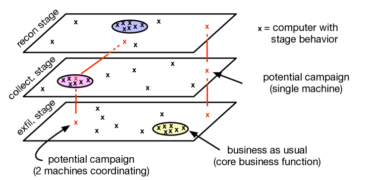
Figure 2: A threat actor’s campaign is often a mix of normal and abnormal activities, and it stands out from benign anomalies if you connect the related risky behaviors. We can view every computer on the network from three perspectives simultaneously: their reconnaissance-like, collection-like, and exfiltration-like behaviors. The points mark computers performing recon-like, or collection-like, or exfil-like actions. In each plane there is a cluster of computers whose core business function, their business-as-usual activities, is to scan, or to collect, or to publish data externally (respectively).

Finally, the solution needs to be transparent so that security analysts can understand what the detection system is doing and the information it surfaces. They need to understand what the big picture is, what the individual activities are that make up the big picture, and why the sets of activity should be considered unusual. Further, automated systems are rarely perfect. Network defenders need to be able to sanity check and verify any potential campaigns before starting mitigation. Verification is much simpler and faster if the system clearly communicates the clues and how they fit together.

3.3 Adapt to an Ever-Changing Environment

In addition to being automated, the solution must be designed to adapt to changing network environments without grandfathering in pre-existing campaigns. A static solution will quickly become stale and ineffective. This has several implications:

• The solution should support using a variety of raw data sources to get visibility into as much of the network as possible. This is necessary to adapt to changing networks. For example, a company that starts running servers on cloud infrastructure (in addition to running servers on premises) will want to extend monitoring to include unusual traffic for those servers. This is straightforward if new data sources, like cloud flow logs, can be added to the system.

• The machine learning components must train on data in situ, to understand what is expected and consistent for each individual network.

• Machine learning models must be retrained and updated frequently to stay relevant. E.g., daily. Otherwise the understanding of what is normal can become outdated as the network evolves in response to organizational requirements.

• Therefore, the training of models must be automatic and not require human intervention. Nobody wants to babysit the system.

• Because the system is trained on data in situ, and because a threat actor may already be in the network, the machine learning models must not grandfather malicious activity as normal. This was a shortcoming of learning systems in the past.

3.4 Hard for Threat Actor to Avoid

It should be hard for a threat actor to avoid detection.

The system should support using multiple log data sources when they are available. Using multiple data sources makes it hard to hide. The more data sources across and within each campaign stage, the greater the ability to detect insiders and persistent threats. It also significantly increases the cost for a threat actor to hide, alter, or remove evidence of activities—particularly when they vary per organization. And threat actors have finite resources.

Similarly, the solution should prefer to use network and server logs when possible. It is harder to avoid leaving clues in network logs and server logs than in client logs. Network and server logs tend to be stored on well-secured devices that are further from the perimeter. Accessing these logs for deletion or modification is trickier.

The system, as a whole, must understand that the majority of individual anomalies are benign and avoid presenting all of them to security analysts. Otherwise a threat actor can hide in the flood of false alarms.

Finally, it should be hard (time consuming and/or expensive) for the threat actor to influence what the machine learning models learn. If the threat actor can manipulate the analysis, they can create blind spots to hide in.

4 How esINSIDER Works

esINSIDER focuses on your data, specifically detecting discovery, access, and movement behaviors that fit the model of a threat actor’s campaign.

4.1 Overview

esINSIDER is a data processing and analysis engine that detects potential adversary campaigns. It is a software-only product that consumes log data, from multiple data sources, that is stored in a data lake [41]. Every day, esINSIDER ingests raw information from the data lake, updates activity profiles for each host on the network, and updates machine learning models of normal activity levels. The activity profile is a set of statistics that summarize the host’s activities over days or weeks. The machine learning models monitor the profiles for anomalies related to reconnaissance, collection, or exfiltration. esINSIDER surfaces relationships in the data that match multiple stages of the adversary campaign lifecycle. To do this, it correlates anomalies across campaign stages and across associated computers to produce cases. Each case summarizes the potential campaign and explains why the hosts and traffic are of interest and add up to a risky narrative.

Before we describe esINSIDER in more detail, we first summarize how the design meets the requirements from Section 3:

• The system is built on top of existing log data sources, with a flexible data pipeline. This makes it easy to incorporate new log sources, as network configuration changes (adaptable). It makes hiding in the network harder and a unique challenge for each site (hard to avoid).

• Monitoring targets, that embody unavoidable adversary campaign behaviors, are derived from log data (mission focus).

• Activities are monitored over long time windows because sophisticated campaigns unfold over weeks or months (mission focus). This increases the cost for the threat actor to avoid detection (hard to avoid).

• Monitoring models are built and updated using machine learning every day. They are learned from the organization’s data so that they are customized to that network and represent what is normal for that network (automated, adaptable, hard to avoid).

• The monitoring models take as inputs contextual information about the host and its activity so that the definition of normal is context-aware (automated). For example, esINSIDER tracks the size of typical data transfers to common external destinations (based on how most computers on the network interact with the destination). This information adjusts the definition for what is a normal data transfer size—per destination.

• The system uses white box machine learning models so we can include reason codes in cases that help explain why an activity is considered anomalous (automated).

• Hierarchical models synthesize anomalous activities to find hosts exhibiting reconnaissance, collection, or data exfiltration behavior (mission focus, automated). Few normal systems in an environment do all of these.

• Cases are generated only when host(s) exhibit high risk for multiple campaign stages (mission focus, automated).

• Cases include the suspicious hosts, their high risk activities, what other computers were involved, and details on the activities (automated).

Now let us examine each part of esINSIDER in more detail.

4.2 From Log Data to Monitoring Targets

The first step in monitoring a network is deciding what is worth measuring. esINSIDER derives monitoring targets from the log data that embody core campaign behaviors.

A monitoring target is a column in a database table that quantifies how much (or how little) each host performed an activity we want to monitor. The concept is easiest to understand by looking at some examples (Table 1). For example, esINSIDER measures the neighborhood of how many internal destinations a host contacted over a month-long time window. This variable aligns with system reconnaissance: small neighborhoods mean low recon risk, and large neighborhoods mean higher recon risk. esINSIDER measures all the monitoring targets (variables) and assesses how unusual and risky each measured value is (see § 4.3). We call the variables targets because of how they are used in the machine learning models (§ 4.3).

Table 1: Example Monitoring Targets

Monitoring Target(s)	Log Source	Visibility Into
How many distinct, internal IP addresses did the host touch over the last month? (via ICMP, SNMP, TCP, UDP)	Flow	Recon (System)
How many distinct, internal IP addresses did the host touch over the last month via dataa, serviceb, and generalc ports?	Flow	Recon (System)
How many distinct, internal reverse DNS lookups (aka, PTR requests) did the host make over the last month?	DNS	Recon (System)
For internal addresses, how many distinct dataa, serviceb, and generalc ports did the host try to connect over (last month)?	Flow	Recon (Service)
How many total bytes did the host consume from every internal address over the last month?	Flow	Collection
How many total bytes did the host publish to every external address over the last month?	Proxy or Flow	Exfiltration
$a$: Data-related ports can be queried for data. E.g., 21 (FTP), 80 (HTTP), and 156 (SQL).
$b$: Service ports are used by well-known services. E.g., 6660-6670 (IRC).
$c$: General ports are everything else.

Said differently, monitoring targets are signals that can be used to detect signs of a campaign using reconnaissance, collection, and exfiltration. Unlike most network security approaches, we deliberately use a small number of monitoring targets (less than 25). Each monitoring target should measure activities that embody fundamental campaign behaviors.

It is worthy clarifying the relationship between behaviors and activities (and therefore, monitoring targets) in esINSIDER. A behavior is an abstraction, a category, that maps to high-level step(s) in a threat actor’s mission plan. In contrast, an activity is something that actually happened on the network. It is concrete and observable. A behavior can be exhibited through different types of activities. For example, there are many ways to exfiltrate data, including: upload files via HTTP/POST, and a DNS covert channel [31]. Each monitoring target summarizes one kind of activity. As a result, esINSIDER typically uses multiple monitoring targets per campaign stage (behavior). This is especially true for reconnaissance because there are sub-behaviors that reflect sub-goals:

• System reconnaissance: discovering what devices are on the network.

• Service reconnaissance: discovering what services target computer(s) are running.

• Data reconnaissance: discovering what information is available in a data store, like the local file system or a SharePoint site.

and because there are multiple good tactics to use for those sub-goals.

Computing the monitoring target values is a large scale data processing problem. Log data can be huge for large organizations. For example, one of our customers generates 12 TB of logs per day (600 GB compressed). Suppose we wanted esINSIDER to analyze the last four weeks of activity and compare it to the preceding four weeks of historical data (to get a better baseline for activities). That means ingesting, distilling, correlating, and making sense of 56 days of data, or 672 TB for this customer.

To handle this scale of data, esINSIDER is built on top of Apache Spark [43] and runs on a distributed compute cluster. The required data transformations distribute well, allowing esINSIDER to scale horizontally. To handle larger log data, just run esINSIDER on a larger cluster. The compute cluster can either run on hardware the customer owns (on prem) or on cloud infrastructure (e.g., Amazon’s Elastic Cloud Computing). To access the log data, esINSIDER reads in raw log data from a data lake in HDFS or in Amazon’s cloud storage (S3). Log files are expected to be organized into date-partitioned folders. E.g.,

    flow/20180520/00.txt.gz
    flow/20180520/01.txt.gz
    flow/20180521/00.txt.gz
    flow/20180521/01.txt.gz
    flow/20180521/02.txt.gz
    flow/20180521/03.txt.gz

A multi-step data pipeline turns the log data into the desired monitoring targets. The log files are parsed to extract fields and create a structured, tabular data set. Next, fields are standardized, to ensure things like consistent casing and timestamp formats. Importantly, this includes mapping dynamic IP addresses to consistent, stable machine names—a requirement for reliably tying together activities that span weeks. After standardization, data are transformed to get them ready for aggregation. This includes many things, but generally the purpose is to label the records with various categories that are used to divide the data during aggregation. For example, flow records are labeled as traffic to internal vs. external destinations and categorized into semantic port groups. (The port groups are defined based on their value to the threat actor: what data can be accessed; what network information can be learned; or system liveness. All of this is reconnaissance but differing in intention, effort, and the value returned to the threat actor. See also Table 1.)

Aggregation happens in two steps. The initial aggregation computes activity statistics that summarize the latest day of records. The final aggregation combines the single day aggregates to get aggregate statistics over a window of days. With some care in the implementation, the windowed aggregates can be computed in time that is independent of the window duration. These multi-day statistics, computed for every device on the network, are the monitoring targets.

There are several benefits from aggregating, with little downside for the use case of detecting campaigns. Aggregation provides a smoothing effect that gets rid of noise: instead of seeing every random spike as an anomaly, esINSIDER detects aggregate outliers. This makes it easier to see the trends that matter. Further, while low-and-slow campaigns [38] are hard to observe over an hour or a day, over time the activities accumulate and become increasingly obvious and anomalous. And of course, the scalability benefits from data reduction are massive. The aggregated data are smaller and easier to do advanced analysis on. For the customer mentioned above, the single day aggregates are 1% the size of the raw logs (7 GB vs. 600 GB, both compressed). The main downside to aggregation is losing fine-grained information about when activities happened. Instead of pinpointing the minute when a campaign action occurred, esINSIDER identifies the host(s) and the day(s). This is enough information to pivot to a SIEM or system of record for the relevant raw logs, and esINSIDER can generate the appropriate queries to drill into findings and submit them to these systems. A second drawback to this aggregation strategy is a longer delay between when the anomaly happens and when it is detected and shown to security analysts. This is because monitoring targets are updated on a daily cadence. Given our focus on campaigns that span weeks or months, a 24 hour delay seems acceptable.

Finally, integrating new data sources is straightforward. (See § 3.4 for why using multiple data sources is valuable.) Data pipelines are specified as graphs of data flowing between reusable transformation blocks. The graphs are defined using a domain-specific language. The block-based data processing is a kind of flow-based programming [42]. esINSIDER can be extended both by defining new processing blocks and by defining new data pipelines.

4.3 Using Machine Learning to Understand Normal

Once we have a monitoring target, we need to decide which of the values are unusual and are worth highlighting as more likely to belong to an adversary campaign than a benign business function. Our approach is to build a monitoring model using machine learning; this model predicts the expected values for a monitoring target. Then we compare the predicted values with the actual values to identify surprising activities. If there is a large discrepancy between predicted and actual values, that means the actual value is unexpected according to the definition embodied in the model. In order to make accurate predictions that account for nuances of the host and its activity, the models use context as inputs to reduce false positives.

A key benefit of this approach is that we can leverage supervised machine learning to solve an anomaly detection problem. Supervised learning simply means that the correct answer is provided to the algorithm that builds the model. Specifically, the learning algorithm looks at labeled example records—with input values and the correct output (target) value—and estimates a function that maps from inputs to the output. The estimated function is the learned model that can be used for predicting target values.

Normally a lot of work is required to label data with the correct answers, but in this application we get them for free. The correct answer—what actually happened—is right there in the logs. We just need to transform and aggregate the logs into the measurements we care about monitoring. Then, every day, esINSIDER analyzes the previous day’s monitoring target values to detect surprising values. The models to do that are learned using the monitoring target values from the day before that.

4.3.1 Digression: What if the Labeled Data are Dirty?

When we learn these models, we must assume that the labels are imperfect, aka dirty. We expect to find benign, one-off outliers in network data that cannot be predicted. Even more concerning, a threat actor may already be in the network, and some labels reflect their campaign actions from the previous days, weeks, or months. The models of normal need to be constructed in a way that avoids treating pre-existing, active campaigns as legitimate, normal network behavior.

Our primary strategy for solving this challenge is to setup the machine learning problems in a way that prevents the model from memorizing the patterns of individual computers. First, there is a single shared model per monitoring target (vs. one model per computer on the network); model learning gets low error by producing accurate predictions for the whole network, not just individual machines. Second, we avoid model inputs (context) that are unique identifiers for machines because they would give the shared model enough degrees of freedom to memorize each device separately. For example, esINSIDER never uses the name or IP address of the device as a model input. Instead, inputs are selected that might be useful for predicting the activity of multiple machines. Third, the automatic feature engineering in esINSIDER (see Appendix A) uses minimum sample sizes to ensure each derived feature is relevant for predicting how a pool of machines behave.

Another way to think about this is that we always want to compare a machine $M$’s activities to a group of computers. Sometimes the comparison group is the whole network (if none of the model inputs provide useful context), and sometimes the group is the set of computers that share some property with $M$ (see § 4.3.2 for examples).

4.3.2 Building Contextualized Monitoring Models

Because the goal is to predict a numeric value, like the expected number of bytes collected, esINSIDER uses non-parametric regression learning. A regression model predicts a numeric value, as a function of some inputs. There are dozens of ways to learn simple or complex regression models from data, including linear regression and neural network algorithms. esINSIDER uses a sophisticated non-parametric learning algorithm that is fast, scalable, transparent, and able to learn non-linear relationships. It includes automated feature engineering for finding informative representations of numeric and string-valued inputs (context). Appendix A describes this learning algorithm in more detail.

After a monitoring model is learned, it is used to predict the target values (aka, activity levels) for all devices on the network and score their risk. For example, the collection model predicts how many total bytes each host consumed from every internal device during the last month. Each prediction sets the expected (normal) value, and this in turn determines the probability of seeing a value as large as the actual target value (see Figure 3). esINSIDER then scales the probability to improve robustness and to better focus on the activities subject matter experts consider most relevant to detecting adversary campaigns.

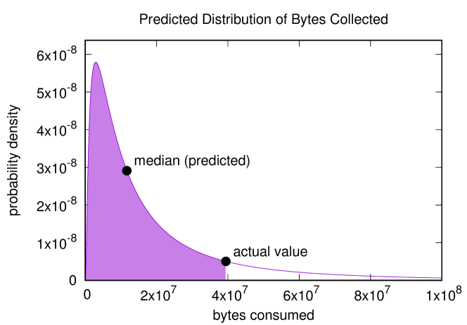
Figure 3: Actual values for a monitoring target are compared to the expected (aka, predicted) distribution to determine how surprising they are. The further right the value lies in the distribution, the more surprising it is. For example, the distribution above corresponds to the stage 4 collection model predicting 11.7MB collected, compared to 39.4MB actually collected. The probability of seeing a more extreme value than 39.4MB is 0.15 (the unshaded area of the distribution). The location (median) and shape of the predicted distribution depend on the contextual inputs.

Accounting for context, in the form of model inputs, is critical for understanding what is normal for approved business functions. A model using context has a more nuanced and multi-faceted view of business-as-usual. Figure 4 shows two examples resulting from running esINSIDER internally on eSentire’s network.

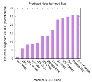
(a) Stage 3 example.

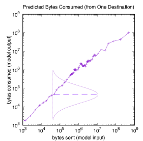
(b) Stage 4 example.

Figure 4: The expected activity (model output) changes based on context (model inputs). These graphs show how the expected activity changes as a function of one particular input, after marginalizing over all other model inputs [10, p. 359]. (4(a)) The expected neighborhood size ranges from 1 neighbor to 20+, depending on the computer’s CIDR block (network segment). (4(b)) The expected bytes collected by a computer varies greatly based on the number of bytes sent. At 40 KB sent, the model predicts 50KB consumed. Overlaid is the predicted distribution (see Figure 3). It would be suprising if the computer collected 10MB while sending 40KB in response. In contrast, 10MB collected would be expected if 10MB had been sent.

On the left, Figure 4(a) shows how many internal neighbors a computer $M$ is expected to talk to as a function of $M$’s CIDR block (network segment). At the low end, computers in Dev AWS typically communicate with a single neighbor; this is because our software development process involves engineers allocating a development machine in EC2 and then tunneling into it. Computers in other CIDR blocks communicate with more neighbors, with the most connected computers performing infrastructure and server roles (e.g., Services, Test, etc.). On the right, Figure 4(b) shows how the expected bytes collected by a computer $M$ from another computer changes based on the traffic going in the other direction (bytes sent). This is because most network traffic involves two-way communications. In all cases, context can change the location and shape of the predicted distribution (recall Figure 3), which leads to different actual values being considered surprising. One example distribution is overlaid in Figure 4(b).

Context is also a way to explain evidence to analysts reviewing a case. For each predicted value, esINSIDER generates reason codes that explain which inputs most strongly influenced the prediction. For example, Figure 5 shows one piece of evidence from testing esINSIDER internally with a simulated campaign. The list of reason codes enumerate the factors driving the prediction and tell users some context supporting why the actual value was surprising.

10.42.28.17 collected $\underbrace{\text{3.20 GB}}_{\text{actual value}}$ from 10.42.24.15. esINSIDER predicted $\underbrace{\text{10.10 MB}}_{\text{expected value}}$ because: 1. baseline prediction was 338.22 KB without context, 2. 15.03 MB were sent to 10.42.24.15 [26.27x multiplier] 3. 10.42.28.17 is in the Users CIDR block (10.42.28.0/22) [1.83x multiplier] 4. collected from 10.42.24.* [0.62x multiplier]

Figure 5: Example evidence with reason codes.

Many kinds of contextual information are useful for understanding what are expected business activities, including:

• Attributes about the device, or its role in the network. E.g., CIDR block labels as in Figure 4(a) (for segmented networks), or the security groups a cloud instance belongs to. These help define peer groups, that is, sets of devices that should behave in similar ways due to similar functions (DB clusters, ETL systems, mail servers, clients, etc.).

• Symmetric byte flow volumes, as shown in Figure 4(b).

• The historical activity for the device. E.g., to predict the number of internal PTR requests (reverse DNS lookups) made over a month, look back at how many were made during the previous month. The historical time window and monitoring time window do not overlap.

• How other computers in the network tend to communicate with a common destination. A common destination is an internal or external server (or cluster of servers with similar network addresses) to which many computers on the network talk. For example, if a company used CrashPlan for offsite backups, uploading large data volumes to code42.com could be normal and expected—and that can be discovered as a pattern because there is a peer group of computers using that external service in similar ways.

Some context comes from joining in extra data sets, while other context inputs need to be computed from the raw logs using the same kinds of data pipelines that compute the monitoring targets.

4.4 From Evidence to Cases

At this point, we have monitoring models and can use them to score activities, for every device. The remaining work is to synthesize this information and build cases.

esINSIDER first computes the stage-level risk scores for each individual device to get an aggregated picture of campaign stage behaviors. The stage risk scores quantify the total reconnaissance, collection, and exfiltration risk for each device, accumulated from the scored activities in each stage. For each stage, esINSIDER builds a stage-level risk model, called a ComboModel, that synthesizes the outputs of the relevant monitoring models. The ComboModel is a kind of hierarchical mixture of experts ensemble model [34]. The current ComboModels are simple by design, using one or two layers of addition and expert-defined weights to compose the monitoring models (Figure 6).

(a) Reconnaissance ComboModel

(b) Collection or exfiltration ComboModel

Figure 6: ComboModels combine outputs from monitoring models into stage risk scores for a computer $X$. The monitoring models $M_{i}$ output the surprise scores $s_{i}$. (6(a)) The reconnaissance ComboModel performs a weighted addition of the surprise scores to get the total stage 3 risk. (6(b)) The collection and exfiltration ComboModels apply two levels of weighted addition to get the stage 4 and 5 risk scores. In the first level, monitoring models score the data flow for each destination (remote) device that $X$ talked to. These are combined to get a risk $R()$ for the destination across all the monitored targets. (Typically, there is one target per data source that captures flow information.) The second level synthesizes the risk across all destinations, to get a total stage 4 or 5 risk for $X$.

Recall that high risk for a single campaign stage is insufficient for detecting potential campaigns with low false positives. Network devices often rank high on risk for a single stage. esINSIDER should not be surprised, for example, if a backup server scored high for data collection. This is normal behavior for a backup server, and it should be ignored. It is much less common for a machine to rank high for two campaign stages, and it is exceedingly rare to score high for all three. When that happens, we have high confidence that the machine is acting suspiciously and should be investigated. Conversely, threat actors need to execute most or all of the recon, collection, and exfiltration stages to complete their campaign mission (§ 3.1), and it is costly for threat actors to hide from detection in all campaign stages.

Consequently, esINSIDER integrates the stage-level rankings to get a single ranking, with the highest risk devices at the top of the ranking. esINSIDER uses the top-ranked devices as the starting points for building candidate cases (see below). Internally, the total ranking score is computed as the geometric mean of the device’s stage-level rankings. Let $r_{i}$ be the rank position for campaign stage $i$. Then:

total ranking score $$=\mathrm{geomean}(r_{3},r_{4},r_{5})=\left(\prod_{i=3}^{5}r_{i}\right)^{\frac{1}{3}}=\sqrt[3]{r_{3}r_{4}r_{5}}$$ (1)

and ranking scores are sorted in ascending order.

We use the geometric mean because it is robust to a small number of large values. We want to ensure any devices with high risk in two campaign stages are ranked high overall. For example, if a computer had the first, tenth, and thousandth highest stage risk scores, its stage rank positions would be 1, 10, and 1000, and its total ranking score would be 21.54. In comparison, the normal arithmetic mean of 1, 10, and 1000 is 337. The single stage with low ranking (1000) dominates the result and obscures the fact that the device ranked high in risk for two stages (1 and 10).

At this point we have a ranked list of all the devices based on the accumulated evidence of all their monitored activities. You could make simple cases from this ranking, where each case consists of a single machine. Frequently though, more than one machine is involved. Threat actors have become increasingly adept in recent years at mounting campaigns that coordinate multiple machines, with some used for recon, others for collection, and a third group for exfil. Therefore, when considering a high ranked device $M$, esINSIDER also examines the risk profile of other machines with interesting relationships to $M$.

Multi-machine threat linking works as follows. Starting from the highest ranked computer, esINSIDER builds a candidate case where that machine is the seed, or starting point, for the case. esINSIDER then adds other computers to the candidate case, where:

• those computers received high or medium risk stage scores, and

• the computers are immediate neighbors, reachable from the seed computer in the association graph.

The association graph contains one vertex per machine, and each edge connects machines where there is an interesting relationship that might indicate campaign coordination (e.g., Figure 7). Like the monitoring targets, the association graph summarizes activity over a window of time. The candidate case includes all the suspicous activities (as determined by the monitoring models) for all the machines in the case. This process is repeated for the second, third, fourth, etc. ranked computers, using each as a seed for generating a candidate case.

The definition for association / coordination is flexible, and this is one of the extension points for esINSIDER. The default functionality is to add a directed edge when there is a surprisingly large data movement between the machines (i.e., the communication between them gets high risk for data collection). The edge points in the direction of the data movement.

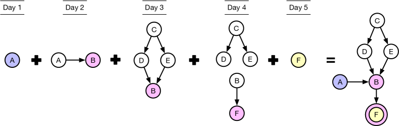
Anomalies
Day Host Stage Activity 1 A 3 laptop $A$ contacts 73 machines on ports 22 (ssh), 110 (pop3), 139 (smb), 143 (imap), & 445 (smb) 2 B 4 server $B$ consumes 50 MB from $A$ 3 B 4 server $B$ consumes 600 MB from $D$ and 3 GB from $E$ 4 F 4 HR workstation $F$ consumes 120 MB from $B$ 5 F 5 uploads 120 MB to external server

Figure 7: esINSIDER links together related suspicious computers to build holistic cases. This example shows five anomalies and the building of the related association graph (top right). Colored circles represent computers showing anomalous activity on the given day. On days 3 and 4, there are large-but-expected data movements from $C$ to $D$ and $E$. The final case would contain $A$, $B$, and $F$ as suspicious computers.

For example, in Figure 7 there are three suspicious computers to use as seeds for threat linking: $A,B,$ and $F$. These result in candidate cases that contain $\{A,B,F\}$, $\{B,F\}$, and $\{F\}$, respectively.

The candidate cases have high total risk—potentially accumulated from risky behaviors on multiple machines—but they are not guaranteed to include high risk for multiple campaign stages. Therefore, in the final step esINSIDER filters the candidate cases, keeping those that contain high risk activities for at least two campaign stages.

5 Conclusion

To detect persistent and insider threats, with a reasonable amount of resources, there are four fundamental requirements:

• Focus on the threat actor campaign goals. Adopting a threat-actor-centric approach clarifies what the core campaign behaviors are, making it easier to see past the tremendous variations in tools and techniques.

• Automate as much as possible, including cross-correlating signals and behaviors, but also make the solution transparent to help security analysts separate persistent and insider threats from business-as-usual and acceptable noise.

• Adapt gracefully to an ever-changing environment and be robust to changes in threat actor tools and techniques to accomplish their campaign mission.

• The detection system needs to be hard for a threat actor to avoid. This includes: using as many reliable, complementary data sources as possible; only showing analysts a small number of high confidence detections; and ensuring threat actors cannot easily influence what the machine learning models learn.

esINSIDER is designed from first principles to meet these requirements. Whereas other tools generate hundreds or thousands of individual alerts per day with arbitrary weighting for risk, esINSIDER’s goal is to track multiple events across multiple adversary campaign behaviors and surface just a handful of cases per week. These cases should be high value because it is unlikely for a correctly behaving system to exhibit multiple campaign behaviors by accident.

To build a case, esINSIDER correlates anomalies across campaign stages and links together associated, suspicious computers—without requiring input from a security analyst. The solution is dynamic and adapted to the network being monitored: machine learning models are learned from the network data (vs. pretrained and shipped with the software), and are updated daily. The case summarizes the findings so that a security analyst can triage, verify, and launch a deeper investigation quickly.

This approach is an important addition to a cybersecurity portfolio, complementing prevention and rapid intrusion detection & response.

Appendix A Automated Learning of Expressive, Transparent Models

The eSentire learning library (esLL) takes labeled, tabular data and returns a model that can predict what labels should be for future data records. The data table contains a target column (the labels, aka, correct answer) and columns to use as model inputs. The inputs can be, and usually are, a mixture of numeric and string-valued columns. The data table can be large and stored in a distributed data structure in the memory of multiple computers in a compute cluster.

A.1 Terminology

This appendix uses the following terminology.

Input

An input signal to a esLL model (Figure 9). A column from a data table that contains potentially useful information for predicting the modeling target.

Feature

A column in a matrix that is used as an input signal for a linear model.

Sparse Matrix

A data matrix that stores the non-zero values only. When most of the values in a matrix are zero, using a sparse representation results in significant memory, and sometimes computational, savings. For example, this matrix with three data records and five features:

$$\begin{bmatrix}1&0&0&0&0.5\\ 0&0&-2&0&0\\ 0&-1&1&0&0\end{bmatrix}$$

can be compactly represented by storing the indices and values of non-zero entries:

1:1 5:0.5
3:–2
2:–1 3:1

A.2 Background

Before we can summarize the underlying learning algorithm, we need to first review linear regression models and their limitations. A linear regression model is a function of the $p$ input features $\vec{x}=x_{1},x_{2},\ldots,x_{p}$, where each feature is multiplied by a weight coefficient $\beta_{j}$:

$$y =f(\vec{x})=\beta_{0}+\beta_{1}x_{1}+\beta_{2}x_{2}+\cdots+\beta_{p}x_{p}=\beta_{0}+\sum_{j=1}^{p}\beta_{j}x_{j}$$ (2)

For the simple case of $p=1$, we end up with

$$y =f(x_{1})=\beta_{0}+\beta_{1}x_{1}$$ (3)

which is the equation for a line with slope $\beta_{1}$ and intercept $\beta_{0}$. These models are called linear because the function is linear in the parameters: increase (or decrease) $x_{j}$, and $y$ changes by a proportional, linear amount.

Linear models have much to recommend them. There are multiple, well-studied methods for estimating (aka, learning) the weight coefficients $\vec{\beta}$ from data [20, 19, 25, 29, 11], including large scale data (large in terms of number of rows $n$ and number of features $p$) [1, 3, 7]. For truly massive data, there are good algorithms for distributing the learning computation across a compute cluster to parallelize the work and achieve nearly ideal scaling [6, 22, 28]. These models are also wonderfully transparent: the model’s equation can be printed out and studied [17]. Further, individual predictions can be understood by inspecting the input values $\vec{x}$ and the weights $\vec{\beta}$, and looking for the largest factors (aka, terms) in the equation [26].

The main limitation of standard linear models is lack of expressiveness: there are many functional relationships $y=f(\vec{x})$ we would like to learn that are not linear. For example, what if the input is a string and not a number: we cannot multiply a string-valued $x_{j}$ by a weight coefficient. What if the relationship between $x_{j}$ and $y$ is quadratic, logarithmic, or a step function? What if the true, unknown relationship is defined by two inputs interacting with each other? The assumption of a linear relationship leads to inaccurate models in these kinds of situations.

However, there is a well known solution to extend the expressiveness of linear models. If we preprocess the data, we can change the representation of the functional relationship into one that does have a linear structure. All of the examples above can be modeled well with a combination of data preprocessing and linear regression (see Table 2).

Table 2: Standard Preprocessing Tricks

Scenario	Strategy
String Input	Encode the string values as a set of binary indicator features, with one feature per string value. For example, if the input is network protocol with possible values of TCP, UDP, and ICMP, then create three features where $(x_{1},x_{2},x_{3})=(1,0,0)$ when the value is TCP, $(0,1,0)$ for UDP, and $(0,0,1)$ for ICMP.
Logarithmic Function	If the relationship between $y$ and $x_{1}$ is logarithmic, add feature $z_{1}=\log(x_{1})$ to get model $y=\beta_{0}+\beta_{1}x_{1}+\beta_{2}z_{1}$.
Polynomial Function	If the target is not a linear function of $x_{1}$ but instead a polynomial function, define appropriate features that are polynomial expansions of $x_{1}$. For example, let $z_{1}=x_{1}^{2}$, $z_{2}=x_{1}^{3}$, and $z_{3}=x_{1}^{4}$. Then the expanded linear model would be $y=\beta_{0}+\beta_{1}x_{1}+\beta_{2}z_{1}+\beta_{3}z_{2}+\beta_{4}z_{3}$.
Interacting Inputs	Add interaction features to the data set. For example, the XOR function can be learned if we add feature $z=x_{1}x_{2}$ to the data set and say the model’s output is 1 when $y>0$ and 0 otherwise. Specifically, it can be solved by $y=0.5x_{1}+0.5x_{2}-1.0z_{1}$.

A.3 The Learning Pipeline

We are now ready to describe the learning algorithm in the esLL. The algorithm combines smart data preprocessing (sometimes called feature engineering) with a core that learns generalized linear models. This combination can learn non-linear models from large scale data containing both numeric and string inputs. Because the data transformations are explicit and the core linear model is transparent, these models can be inspected, and we can generate reason codes that explain the factors that underlie any given prediction (e.g., Figure 5). Importantly, many decisions about data preprocessing can be decided automatically by the esLL.

Figure 8 illustrates the steps in the learning pipeline. Beforehand, the labeled data are split into two subsets, a training data set and a tuning data set. The training data are used to learn model weights, and the tuning data are used to choose which model, out of many possible variations, is the best.

Figure 8: The learning pipeline in esINSIDER is a combination of smart data pre-processing and learning linear models. Many variations are possible at each stage, resulting in many possible branches. See sections A.3 and A.4 for details.

The dense transform pipeline transforms the data using a series of table transforms. These are operations that take a data table as input and produce a new data table with new or modified columns. Unlike the matrix transforms (see below), this part of the pipeline has maximum flexibility for massaging the data. For example,

• String and timestamp columns can be manipulated directly, without special encoding. For example, a transform could extract the day of week and whether that day was a holiday from a timestamp column, creating two new inputs for the model.

• Transforms can compute new columns based on multiple rows. For example, for input data with one row per day per computer, a rolling window transform can compute each computer’s median bytes sent for the previous two months.

• Transform the target column to improve learnability. In esINSIDER, for example, we add a replacement target column that is the $\log()$ of the original target column. (The reason why this helps is technical and outside the scope of this paper.)

In our experience, the table transforms are usually chosen based on subject matter expertise and domain knowledge. Some transforms have parameters that can be tuned automatically based on how it affects model accuracy (e.g., how long should the window be in a rolling window transform).

Next, the learning pipeline encodes the data table into a sparse feature matrix. The goal is to represent all the valuable information in the data table as purely numeric values that are ready for building linear models. This is broken down by input column in the table; for each input, an encoder function is applied to produce a set of sparse features. For example, a simple encoding strategy for string inputs is to generate binary indicator features with one feature per string value (see Table 2). The snippets of features are pasted together to get the full matrix.

Encoding is special in the learning pipeline because a) it always happens, and b) it almost always needs to learn the encoding functions from data. For the example of encoding a string input as a set of indicator features, the esLL collects the set of possible values from the train and tune data and then builds the encoding function from that set. As a second example, a useful encoding strategy for numeric inputs is to sort the values and divide them into equal volume bins, and then have one feature per bin that indicates if the input value was in the bin’s range. The fence posts that set the bin boundaries are function parameters that are learned from the data. How many bins to use can be specified by the library caller, or it can be learned from the data.

There are multiple choices for how to encode each type of input column, and the best encoding strategy depends on the problem and can be different for each input column. The esLL includes the following strategies:

Passthrough Encoder (numeric)

Copy the numeric input values, unmodified, into a single feature column.

Quantile Binning Encoder (numeric)

Compute the quantile statistics (aka, fenceposts) for the input and create one binary feature for each of the discretized ranges (aka, bins).

Tree Encoder (numeric)

Learn a classification or regression tree [4, 33] to predict the target, using only a single numeric input column. The leaves in the tree divide the numeric values into discrete ranges; create one binary feature per tree leaf [15]. This strategy is self-tuning: it learns both the number of bins and the location of bin fence posts automatically.

One-Hot Encoder (string)

See description in Table 2. This works well when the set of possible values is finite and relatively small; e.g., a set of department names or CIDR block labels.

Cluster String Encoder (string)

This is useful when the number of unique string values is large. E.g., the input is the domain on the Internet where data was uploaded. It is a simplified variation of target statistics [24], where smoothing with a prior probability is avoided by requiring a minimum sample size. Target statistics have been used in click prediction problems under the names counting features and historical counts [5, 16, 12, 18].

Cluster the data rows by the string values (one cluster per unique value) and compute the size and average target value for each cluster. The averages represent the typical target value for data belonging to the cluster; intuitively, this should be very informative for predicting the target value. The frequency (cluster size) summarizes how reliable the average is (more frequent observations equals more confidence that the sample average is representative of future observations).

Next, apply the quantile binning encoder twice, once to the set of average values, and once to the frequency values, to generate indicator features that represent ranges of averages and ranges of frequencies. Finally, generate interaction features between the average and frequency features.

esINSIDER uses all of these encoding strategies.

After encoding, the final preprocessing step is applying an optional pipeline of matrix transforms. A matrix transform operates on a sparse matrix to produce a new sparse matrix. The most important matrix transform is the interaction transform, which derives new features by multiplying all pairs of existing features together. Because this includes multiplying a feature by itself, the interaction transform implements both the polynomial and interaction strategies from Table 2. The interaction transform can be applied multiple times to get third, fourth, etc., order polynomials and interactions. E.g., $x_{1}^{2}x_{2}$ would be a third order term generated after two applications of the transform.

The last stage in the learning pipeline is fitting a linear model to predict the target values from the given features. The software uses best practices for fitting robust models:

• Use ridge [23] or LASSO [40] regularization to control overfitting. The regularization hyperparameter is chosen automatically by fitting models with different regularization strengths and keeping the variation with the best accuracy on the tuning data.

• Standardize each feature column in the matrix to have mean zero and standard deviation of 1.

The esLL uses the L-BFGS optimization algorithm [29] when fitting the model coefficients.

Figure 9: Anatomy of a esLL prediction model.

The output of this learning pipeline is a prediction model that is a non-linear function of the inputs (Figure 9). Internally, this model encapsulates all the transformations and encoders that were used during the learning pipeline plus the linear model that operates on the expanded feature space. In contrast to the learning pipeline (Figure 8), all of the processing steps in the model are fixed functions with fixed parameter values. All choices about which encoders and transforms to use, how to parameterize them, and the best model weight coefficients are decided during learning.

The model internally stores the derivation for each feature. This is used to describe the model’s logic and to generate reason codes explaining how the top features influenced a given prediction.

A.4 Automated Exploration

In the learning pipeline there are many modeling decisions to make. Which, if any, table transforms to use? Which encoding strategies to use? What hyperparameter values, e.g., number of bins, should be used? Should feature interactions be added during the sparse pipeline; second order, third order, etc.? Which of the derived features should be kept (because they improve accuracy) and which should be discarded? This section describes how this learning pipeline is setup and controlled to produce good models with minimal human effort.

Traditionally, a modeling expert and/or domain expert would spend weeks experimenting with different pipeline variations, looking for the combination that produced the best result. Even with that time investment, only a small fraction of the possible combinations would be tried. From a usability standpoint, specifying all of the minute controls for the learning pipeline would be tedious and error prone.

The esLL automates the trial-and-error search for a good model while also allowing experts to control as much, or as little, of the learning pipeline as they want. To learn a model, the library is called with a model blueprint, train data, and tune data. The model blueprint is a configuration object that specifies the instructions for defining the learning pipeline and building a model from the data. Many instructions for a model can be left unspecified, and the esLL will fill in the missing instructions using a combination of heuristics and automated exploration to find good fill-in values.

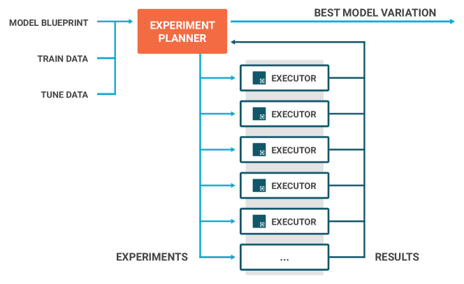
Figure 10: Flow chart for automated exploration.

Figure 10 shows the control flow for this process. An experiment planner takes the incomplete blueprint, generates a set of experiments to run, and schedules them on a pool of executors. Each experiment is a full set of instructions for a learning pipeline: which table transforms, which encoding strategies, which matrix transforms, whether to use ridge or LASSO regularization, and the generalized linear model family to use. In other words, each experiment asks the question of how good the model produced by the particular learning pipeline will be. An executor picks up an experiment, runs the learning pipeline to produce a model, and then evaluates the model’s error rate on the tuning data. The experiment results (the error rates) are sent back to the planner. The planner records the best model found so far (and the instructions used to learn it). Based on the results, it generates new experiments to explore new refinements. This continues until the best model is good enough, the budgeted learning time has expired, every allowed model variation has been tried, or progress stops being made.

Users control the extent of exploration with the time_tradeoff and explorations instructions in the blueprint. The time_tradeoff instruction tells the planner how much time should be spent exploring after learning a first quick-and-dirty model. For greater control, the explorations instruction can be set to define the space of allowed explorations for different part(s) of the learning pipeline. For example, this is used to instruct the experiment planner to try adding interaction features during the sparse pipeline, and how many times to apply the interaction transform.

In summary, the esLL learns quality models by automating the brute force, trial-and-error work that used to be done by human experts. Thousands of variations are tried and evaluated. The net effect of automating the learning pipeline is to automate formulaic feature engineering and allow the human expert to focus on the domain and business problem.

References

- Andrew and Gao [2007] G. Andrew and J. Gao. Scalable training of -regularized log-linear models. In Proceedings of the 24th International Conference on Machine Learning, pages 33–40, 2007.
- Axelsson [2000] S. Axelsson. The base-rate fallacy and the difficulty of intrusion detection. ACM Trans. on Information and System Security, 3(3):186–205, Aug. 2000. ISSN 1094-9224. 10.1145/357830.357849. URL http://doi.acm.org/10.1145/357830.357849.
- Bottou [2010] L. Bottou. Large-scale machine learning with stochastic gradient descent. In Proceedings of COMPSTAT’2010, pages 177–186, 2010.
- Breiman et al. [1984] L. Breiman, J. Friedman, C. J. Stone, and R. A. Olshen. Classification and Regression Trees. Chapman & Hall/CRC, 1984.
- Chen et al. [2009] Y. Chen, D. Pavlov, and J. F. Canny. Large-scale behavioral targeting. In Proceedings of the 15th ACM SIGKDD International Conference on Knowledge Discovery and Data Mining, pages 209–218, New York, NY, USA, 2009. ACM. 10.1145/1557019.1557048.
- Chu et al. [2006] C.-T. Chu, S. K. Kim, Y.-A. Lin, Y. Yu, G. R. Bradski, A. Y. Ng, and K. Olukotun. Map-Reduce for machine learning on multicore. In Advances in Neural Information Processing Systems 19, pages 281–288, 2006.
- Crammer et al. [2012] K. Crammer, M. Dredze, and F. Pereira. Confidence-weighted linear classification for text categorization. Journal of Machine Learning Research, 13:1891–1926, 2012.
- Denning [1987] D. E. Denning. An intrusion-detection model. IEEE Transactions on Software Engineering, SE-13(2):222–232, Feb. 1987. ISSN 0098-5589. 10.1109/TSE.1987.232894.
- Dunwoody and Carr [2016] M. Dunwoody and N. Carr. No easy breach. Presented at DerbyCon 2016 in Louisville, KY, USA., Sept. 2016. Accessed: 2019-02-12. Slides downloaded from https://www.slideshare.net/MatthewDunwoody1/no-easy-breach-derby-con-2016.
- Hastie et al. [2009] T. Hastie, R. Tibshirani, and J. Friedman. The Elements of Statistical Learning. Springer Science+Business Media, New York, NY, USA, second edition, 2009. 12th printing with corrections, Jan 2017.
- Hesterberg et al. [2008] T. Hesterberg, N. H. Choi, L. Meier, and C. Fraley. Least angle and penalized regression: A review. Statistics Surveys, 2:61–93, 2008.
- Hillard et al. [2011] D. Hillard, E. Manavoglu, H. Raghavan, C. Leggetter, E. Cantú-Paz, and R. Iyer. The sum of its parts: Reducing sparsity in click estimation with query segments. Information Retrieval, 14(3):315–336, June 2011. 10.1007/s10791-010-9152-6.
- Hutchins et al. [2011] E. M. Hutchins, M. J. Cloppert, and R. M. Amin. Intelligence-driven computer network defense informed by analysis of adversary campaigns and intrusion kill chains. Leading Issues in Information Warfare & Security Research, 1(1):80–106, 2011.
- Javitz and Valdes [1991] H. S. Javitz and A. Valdes. The SRI IDES statistical anomaly detector. In IEEE Computer Society Symposium on Research in Security and Privacy, pages 316–326, May 1991. 10.1109/RISP.1991.130799.
- Kohavi and Sahami [1996] R. Kohavi and M. Sahami. Error-based and entropy-based discretization of continuous features. In Proceedings of the 2nd International Conference on Knowledge Discovery and Data Mining, pages 114–119, Menlo Park, CA, USA, 1996. AAAI Press.
- Li et al. [2010] W. Li, X. Wang, R. Zhang, Y. Cui, J. Mao, and R. Jin. Exploitation and exploration in a performance based contextual advertising system. In Proceedings of the 16th ACM SIGKDD International Conference on Knowledge Discovery and Data Mining, pages 27–36, New York, NY, USA, 2010. ACM.
- Liao [1994] T. F. Liao. Interpreting Probability Models: Logit, Probit, and Other Generalized Linear Models. Number 101 in Quantitative Applications in the Social Sciences. Sage Publications, 1994.
- Ling et al. [2017] X. Ling, W. Deng, C. Gu, H. Zhou, C. Li, and F. Sun. Model ensemble for click prediction in Bing search ads. In Proceedings of the 26th International Conference on World Wide Web Companion, pages 689–698, Republic and Canton of Geneva, Switzerland, 2017. International World Wide Web Conferences Steering Committee. ISBN 978-1-4503-4914-7. 10.1145/3041021.3054192.
- Malouf [2002] R. Malouf. A comparison of algorithms for maximum entropy parameter estimation. In Proceedings of the 6th Conference on Natural Language Learning, pages 1–7, Stroudsburg, PA, USA, 2002. Association for Computational Linguistics. 10.3115/1118853.1118871. URL https://doi.org/10.3115/1118853.1118871.
- Mandel [1982] J. Mandel. Use of the singular value decomposition in regression analysis. The American Statistician, 36(1):15–24, Feb. 1982.
- Mandiant [2013] Mandiant. APT1: Exposing one of China’s cyber espionage units. Technical report, Mandiant, 2013.
- Mann et al. [2009] G. Mann, R. McDonald, M. Mohri, N. Silberman, and D. D. Walker. Efficient large-scale distributed training of conditional maximum entropy models. In Advances in Neural Information Processing Systems, pages 1231–1239, 2009.
- Marquardt and Snee [1975] D. W. Marquardt and R. D. Snee. Ridge regression in practice. The American Statistician, 29(1):3–20, 1975. 10.1080/00031305.1975.10479105.
- Micci-Barreca [2001] D. Micci-Barreca. A preprocessing scheme for high-cardinality categorical attributes in classification and prediction problems. SIGKDD Explorations Newsletter, 3(1):27–32, July 2001. 10.1145/507533.507538.
- Minka [2003] T. P. Minka. A comparison of numerical optimizers for logistic regression. Technical report, Microsoft, Oct. 2003. Revised March 26, 2007.
- Molnar [2018] C. Molnar. Interpretable Machine Learning. Lean Publishing, 2018.
- Newman et al. [2002] D. Newman, J. Snyder, and R. Thayer. Crying wolf: False alarms hide attacks. http://www.networkworld.com/techinsider/2002/0624security1.html, June 2002. Accessed: 2013-09-29.
- Niu et al. [2011] F. Niu, B. Recht, C. Ré, and S. J. Wright. Hogwild!: A lock-free approach to parallelizing stochastic gradient descent. In Advances in Neural Information Processing Systems, pages 693–701, 2011.
- Nocedal and Wright [2006] J. Nocedal and S. J. Wright. Numerical Optimization. Springer Science+Business Media, New York, NY, USA, second edition, 2006.
- Patcha and Park [2007] A. Patcha and J.-M. Park. An overview of anomaly detection techniques: Existing solutions and latest technological trends. Computer Networks, 51(12):3448–3470, 2007. https://doi.org/10.1016/j.comnet.2007.02.001.
- Piscitello [2016] D. Piscitello. What is a DNS covert channel? https://www.icann.org/news/blog/what-is-a-dns-covert-channel, Dec. 2016. Accessed: 2018-05-21.
- Porras and Neumann [1997] P. A. Porras and P. G. Neumann. EMERALD: Event monitoring enabling responses to anomalous live disturbances. In 1997 National Information Systems Security Conference, Oct. 1997.
- Quinlan [1993] J. Quinlan. C4.5: Programs for Machine Learning. Morgan Kaufmann, 1993. ISBN 1558602380.
- Ruta and Gabrys [2000] D. Ruta and B. Gabrys. An overview of classifier fusion methods. Computing and Information Systems, 7(1):1–10, 2000. URL http://decweb.bournemouth.ac.uk/staff/bgabrys/publications/CIS˙2000˙Ruta˙Gabrys˙fusion˙methods˙overview.pdf.
- Schwartz [2014] M. J. Schwartz. Target ignored data breach alarms. https://www.darkreading.com/attacks-and-breaches/target-ignored-data-breach-alarms/d/d-id/1127712, Mar. 2014. Accessed: 2019-02-12.
- Smaha [1988] S. E. Smaha. Haystack: An intrusion detection system. In Fourth Aerospace Computer Security Applications, pages 37–44, Sept 1988. 10.1109/ACSAC.1988.113412.
- Strom et al. [2017] B. E. Strom, J. A. Battaglia, M. S. Kemmerer, W. Kupersanin, D. P. Miller, C. Wampler, S. M. Whitley, and R. D. Wolf. Finding cyber threats with ATT&CK™-based analytics. Technical Report MTR170202, MITRE, June 2017.
- Symantec [2011] Symantec. Advanced persistent threats: A Symantec perspective. Preparing the right defense for the new threat landscape. Technical report, Symantec, 2011. URL https://www.symantec.com/content/en/us/enterprise/white˙papers/b-advanced˙persistent˙threats˙WP˙21215957.en-us.pdf. https://www.symantec.com/content/en/us/enterprise/white˙papers/b-advanced˙persistent˙threats˙WP˙21215957.en-us.pdf.
- Tavallaee et al. [2010] M. Tavallaee, N. Stakhanova, and A. A. Ghorbani. Towards credible evaluation of anomaly-based intrusion-detection methods. IEEE Trans. on Systems, Man and Cybernetics—Part C: Applications and Reviews, 40(5), Sept. 2010.
- Tibshirani [1996] R. Tibshirani. Regression shrinkage and selection via the lasso. Journal of the Royal Statistical Society. Series B (Methodological), 58(1):267–288, 1996.
- Viswanathan and Hillard [2017] V. Viswanathan and D. R. Hillard. A CISO’s approach to building a successful data lake for cybersecurity and beyond. Technical report, Versive, May 2017. URL https://go.versive.com/versivedatalakewp. https://go.versive.com/versivedatalakewp.
- Wikipedia [2006] Wikipedia. Flow-based programming. https://en.wikipedia.org/wiki/Flow-based˙programming, 2006. Accessed: 2018-05-25.
- Zaharia et al. [2016] M. Zaharia, R. S. Xin, P. Wendell, T. Das, M. Armbrust, A. Dave, X. Meng, J. Rosen, S. Venkataraman, M. J. Franklin, A. Ghodsi, J. Gonzalez, S. Shenker, and I. Stoica. Apache Spark: A unified engine for big data processing. Communications of the ACM, 59(11):56–65, Oct. 2016. ISSN 0001-0782. 10.1145/2934664. URL http://doi.acm.org/10.1145/2934664.
- Zatko [2018] P. Zatko. Artificial intelligence meets mission-focused adversary detection. Technical report, Versive, 2018. URL https://go.versive.com/mudgewp. https://go.versive.com/mudgewp.