Place-specific Background Modeling Using Recursive Autoencoders

Abstract

Image change detection (ICD) to detect changed objects in front of a vehicle with respect to a place-specific background model using an on-board monocular vision system is a fundamental problem in intelligent vehicle (IV). From the perspective of recent large-scale IV applications, it can be impractical in terms of space/time efficiency to train place-specific background models for every possible place. To address these issues, we introduce a new autoencoder (AE) based efficient ICD framework that combines the advantages of AE-based anomaly detection (AD) and AE-based image compression (IC). We propose a method that uses AE reconstruction errors as a single unified measure for training a minimal set of place-specific AEs and maintains detection accuracy. We introduce an efficient incremental recursive AE (rAE) training framework that recursively summarizes a large collection of background images into the AE set. The results of experiments on challenging cross-season ICD tasks validate the efficacy of the proposed approach.

I Introduction

Image change detection (ICD) for detecting changed objects in front of a vehicle as compared with a place-specific background model using an on-board monocular vision system is a fundamental problem in intelligent vehicle (IV). Many researchers recently addressed IV applications in large-scale real-world scenarios (e.g., intelligent transportation systems) rather than small laboratory scenarios [1]. For these scenarios, to train place-specific background models for every possible place can be impractical. It requires very considerable space/time costs proportional to the environment size. The motivation of this study was to enhance model compactness while maintaining the effectiveness of the ICD system.

As a primary contribution, we introduce a new autoencoder (AE) based efficient ICD framework that combines the advantages of AE-based anomaly detection (AD) and AE-based image compression (IC). An AE is an unsupervised neural network that takes an input image and maps it to a hidden representation using an encoder network and then uses a decoder network to reconstruct the input from the hidden representation. Our AE-based approach is motivated by recent successes in two independent research fields: AD [2] and IC [3]. (1) In the field of learning-based AD, it has recently been reported that the reconstruction error of an AE is a very good indicator of anomalous or changed objects [4]. (2) In the field of learning-based IC, the employment of an AE as a compressor/decompressor of input/output images has become a de facto standard [5].

We were particularly interested in the use of place-specific AEs as a basis of ICD and explored their use in this study. Suppose a given sequence of place-specific background images acquired by a vehicle along a known trajectory in the target environment. We aim to partition the background image collection into $N$ disjoint clusters and train a minimal collection of $N$ place-specific AEs $\{c_{1}$, $\cdots$, $c_{N}\}$ from individual clusters. A naive solution would be to partition the image sequence into equal-length subsequences and then train each AE using each subsequence. However, this solution ignores the appearance of background images and their semantic similarity, which may lead to a suboptimal detection/compression performance.

Figure 1: Recursive background modeling. Each panel shows from left to right, viewpoints of all background images, viewpoints of background images that are not well explained by the first, second, and third autoencoder (AE), respectively. Colored horizontal line segments connect the viewpoints explained by each AE.

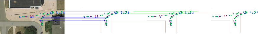
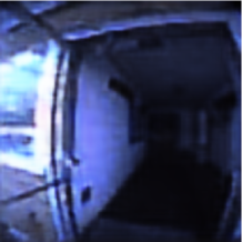
To address the above issues, we propose a novel recursive AE (rAE) training method that exploits the reconstruction error (RE) of AEs as a key measure (Fig. 1). That is, we perform virtual AD using the background image as input to the current AE set. This virtual AD provides two important cues (Fig. 2). (1) If the RE is larger than the allowable error, it is likely that the background image cannot be modeled by the current AE set, indicating the necessity of adding a new AE (i.e., $N_{i+1}$$\leftarrow$$N_{i}+1$). (2) If the RE is sufficiently small for an existing member $c_{j}$$(j\in[1,N_{i}])$ of the current AE set, it can then be used as training data to update the binary normal/anomalous decision boundary of that AE $c_{j}$ (i.e., $N_{i+1}$$\leftarrow$$N_{i}$). Thus, our approach exploits the RE as a single unified measure for minimizing the number of AEs while maintaining the detection accuracy of individual AEs. After the $i$-th AE $c_{i}$ has been trained from a training image set $T_{i}^{+}$, the training set is classified by the current AE set $\{c_{j}\}_{j=1}^{i}$ into a normal subset $T_{i+1}^{-}$ and an anomalous subset $T_{i+1}^{+}$, and then the latter set is used to train the next generation AE $c_{i+1}$ recursively. We implemented the proposed algorithm and verified its effectiveness in a challenging scenario of cross-season ICD using the publicly available North Campus Long-Term (NCLT) dataset [1].

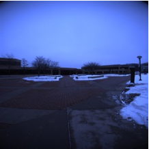
(a) RE = 1.2907

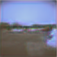
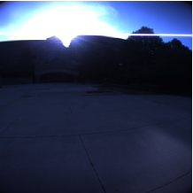
(b) RE = -0.0335

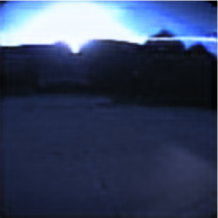
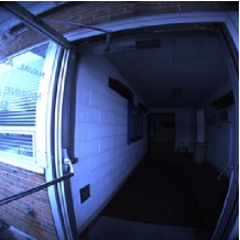
(c) RE = -0.5431

Figure 2: Examples of input and reconstructed image pairs and the normalized reconstruction errors.

II Approach

II-A Problem Formulation

We consider a two stage offline-online framework, where the offline process is responsible for training a minimal set of AEs from a collection of background images, and the online process is aimed to evaluate the likelihood of changes (LoC) for each test image and finally determine whether each test image is change or no-change. We assume that every query live image is correctly paired with a background image beforehand by using a global viewpoint information system such as GPS. We do not assume background images contain only stationary objects, but that dynamic objects may exist even in the background images. We also do not assume the query-background image pair is perfectly registered, but that a non-negligible number of registration errors may exist.

It is noteworthy that the objective of our method is different from and orthogonal to that of ensemble learning (EL) [6]. EL techniques, such as bagging and boosting, have been studied mainly in the context of alternative tasks of classification and clustering to reduce the dependence of the model on the specific dataset or data locality. As compared with that of these classical applications, the effective use of EL in AD is not straightforward because of (1) the unavailability of ground-truth training data and (2) the small sample space problem [7]. The recently developed method presented in [8] is one of very few EL methods in which a set of AEs is employed for AD. However, the paper addressed a single AD problem, not multiple place-specific AD problems, as this paper does.

II-B Evaluating Likelihood of Change

The basic idea of the online ICD process is to reconstruct a query live image $I$ by using its counterpart (or linked) background model (i.e., AE) $c_{j}$, as shown in Fig. 2. The AE is designed to extract the common factors of variation from normal samples and reconstruct them accurately. However, anomalous samples do not contain these common factors of variation and thus cannot be reconstructed accurately. Therefore, the region-level LoC $V_{RE}$ for a given image region $P$ can be evaluated by the RE at each pixel $p$:

$$V_{RE}(P)=\sum_{p\in P}|I(p)-I^{\prime}(p)|,$$ (1)

where the images $I$ and $I^{\prime}$ are the input image and the image reconstructed by the AE that is linked to the corresponding background image, respectively, and $|\cdot|$ is an absolute value operator. If $V_{RE}$ exceeds a pre-defined threshold $V_{RE}^{*}$ (Section II-E), the interest region $P$ is determined as an anomalous object.

II-C Training Autoencoders

The rAE training procedure is described as follows. We first initialize the training set $T_{1}$ with all the available training sets, and set $i=1$. Then, we iterate a process that consists of the following three steps.

Step 1: Given a training set $T_{i}$ we evaluate the RE (i.e., Eq. 1) for each training image $I\in T_{i}$ using the current AE set $\{c_{j}\}_{j=1}^{N_{i}}$.

Step 2: The ID $j^{*}$ of the best AE that gives the minimum RE (i.e., Eq. 1) is assigned to each training image $I$.

Step 3: If the RE value $V_{RE}$ is equal to or smaller than a pre-set threshold $V_{RE}^{*}$ for all the training images $T_{i}^{+}$, the approximation accuracy is considered satisfactory and the iteration is terminated. Otherwise, we return to the Step-1, by setting $i\leftarrow i+1$ and $T\leftarrow T_{i}^{+}$, where $T_{i}^{+}$ is a subset of $T_{i}$ where the RE is greater than $V_{RE}^{*}$.

Our training procedure is partially similar to that of OUTRES [9] in its recursive nature. Whereas most existing EL-based AD methods construct a set of independent models from training data, OUTRES is one of a very few methods that construct models that are interdependent. However, our approach is different from OUTRES in terms of its objective. Whereas OUTRES uses the previous models for refining the current model, we use them for virtual AD to determine whether a new object is well explained by the previous model.

II-D Accelerating Compression

The proposed approach allows accelerated compression of AEs. Suppose we are given two independent AE sets $S$=$\{c_{j}\}_{j=1}^{N}$ and our objective is to obtain a more compressed AE set $S^{\prime}$=$\{c_{j}^{\prime}\}_{j=1}^{N^{\prime}}$, where $N\geq N^{\prime}$. Our approach allows us to use the first $N^{\prime}$ AEs in the sequence $S$ (i.e., $\{c_{j}\}_{j=1}^{N^{\prime}}$) in place of the $N^{\prime}$ AEs in $S^{\prime}$. As a result, when we have a large AE set, we can obtain a smaller AE set, without training a new AE. This property is important in space limited systems, such as archiving and streaming applications.

II-E Normalizing Reconstruction Errors

One design issue of the above training procedure is the determination of the threshold $V_{RE}^{*}$ on $V_{RE}$ for different AEs. Because individual AEs are trained using different training sets, the RE outputs by different AEs are not comparable. To address this issue, we propose normalizing each RE value by the AE-specific normalizer constant.

For the normalization, we approximate the probability distribution function (PDF) of the REs simply by a Gaussian distribution, and normalize the RE value by subtracting the mean value $\mu$ and dividing by its standard deviation (SD) $\sigma$ and by a normalizer coefficient $c$ set at $c=0.8$ in default. This normalization allows outputs from different AEs to be compared and allows their direct comparison.

One desirable property of the SD-based normalizer is that it can be updated incrementally by incorporating new RE value $V_{i}$: $\mu=N^{-1}\sum_{i=1}^{N}V_{i}$, $\sigma^{2}=(N^{-1}\sum_{i=1}^{N}V_{i}^{2})-(N^{-1}\sum_{i=1}^{N}V_{i})^{2}$. This allows us the normal/anomalous decision boundary to be updated incrementally by incorporating new training images.

II-F Ranking Pixels

We now consider the binary decision problem, which takes the list of pixels from all the test query images with their LoC values, and classifies each pixel as either change or no-change. To achieve this, we simply sort the pixels in descending order of the normalized LoC values: the top-$X$ ranked pixels are output as anomalous pixels.

III Experiments and Discussions

We evaluated the proposed rAE-based ICD approach in terms of detection accuracy.

III-A Dataset

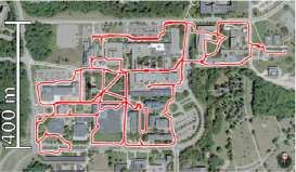
We used the NCLT dataset [1]. This dataset is a large-scale, long-term autonomy dataset for robotics research collected at the University of Michigan’s North Campus by using a Segway vehicle platform (Fig. 3). The data used in our study include view image sequences along the vehicle’s trajectories acquired by the front facing camera of the Ladybug3.

Figure 3: Experimental environment and vehicle trajectories.

From the viewpoint of the ICD benchmark, the NCLT dataset has desirable properties. It includes various types of changing images such as those of cars, pedestrians, building construction, construction machines, posters, and tables and whiteboards with wheels, from seamless indoor and outdoor navigations of the Segway vehicle. Moreover, it has recently gained significant popularity as a benchmark in the robotics community [10].

In the current study, we used four datasets “2012/1/22,” “2012/3/31,” “2012/8/4,” and “2012/11/17” (hereafter, referred to as WI, SP, SU, and AU, respectively) collected across four different seasons, and annotated in the form of bounding boxes (BBs) 986 different changed objects in total that are found in all the possible 12 pairings of query and database seasons (i.e., $\{(i,j)|$$i,j\in\{WI,SP,SU,AU\},i\neq j$$\}$). In addition, we prepared a collection of 1,973 random destructor images that do not contain changed objects and are independent of the 986 annotated images. Then, we merged these 1,973 destructor images and 986 annotated images to obtain a database of 2,959 images.

III-B Performance Metric

Performance on the ICD task was evaluated in terms of top-$X$ accuracy. First, we estimated the LoC image by applying an ICD algorithm. We then impose a 2D grid with $10\times 10$ pixel sized cells on the query image and estimated the LoC for each cell by max-pooling the pixel-wise LoC values from all pixels that belong to that cell. Next, all the cells from all query images were sorted in descending order of LoC value, and the accuracies of the top-$X$ items in the list were evaluated. We evaluated the top-$X$ accuracy for different $X$ thresholds in consideration of the intersection-over-union (IoU) criterion [11]. For a specific $X$ threshold, a successful detection was defined as a changed object, the annotated BB of which was sufficiently covered (IoU $\geq$ 50% or 25%) by the top-$X$ percent of cells.

III-C Comparing Methods

We also compared the performance of the proposed method with that of two benchmark methods: nearest neighbor anomaly detection (NN) [12], and AE with k-means -based place clustering (k-means) [13].

The NN method measures the LoC of a query feature by its dissimilarity to the most similar background feature. First, every query/background image is represented by a collection of SIFT features with Harris-Laplace keypoints [14]. Then, the LoC at each keypoint in the query image is measured by the L2 distance between a SIFT descriptor at that keypoint and its nearest-neighbor-SIFT in the database image.

The k-means method is different from the proposed method (AE) only in that it employs k-means clustering in the space of CNN features instead of the proposed clustering method. Each of the $k$ trained AEs was used as the background model of the background images that belong to the cluster.

III-D Performance Results

Table I shows the performance results for IoU$\geq 25$ and IoU$\geq 50$. We can see that the proposed method outperforms both the k-means and the NN methods in almost all the considered cases. Among the compared methods, the performance of the k-means’s method was the second best. NN showed the poorest performance. One reason for this is that it produced a number of small region proposals and tended to be affected by minor appearance changes between the query and background scenes. In contrast, the proposed method succeeded in producing a precise pixel-wise anomaly score by using the AE set was trained to cover the collection of background images.

TABLE I: Performance results in Top-$X$ accuracy [%].

$X$	rAE		k-means		NN
	$\geq$25	$\geq$50	$\geq$25	$\geq$50	$\geq$25	$\geq$50
5	7.5	2.4	7.3	1.9	0.0	0
10	17.8	5.5	17.1	3.7	3.2	0
15	29.3	10.5	28.6	8.3	22.0	0
20	41.3	14.7	40.3	13.2	46.0	1.0

References

- [1] N. Carlevaris-Bianco, A. K. Ushani, and R. M. Eustice, “University of michigan north campus long-term vision and lidar dataset,” The International Journal of Robotics Research, pp. 1023–1035, 2015.
- [2] V. Chandola, A. Banerjee, and V. Kumar, “Anomaly detection: A survey,” ACM computing surveys (CSUR), vol. 41, no. 3, p. 15, 2009.
- [3] J. Ballé, V. Laparra, and E. P. Simoncelli, “End-to-end optimized image compression,” arXiv preprint arXiv:1611.01704, 2016.
- [4] G. Hinton and R. Salakhutdinov, “Reducing the dimensionality of data with neural networks,” Science, vol. 313, no. 5786, pp. 504 – 507, 2006.
- [5] R. Torfason, F. Mentzer, E. Agustsson, M. Tschannen, R. Timofte, and L. Van Gool, “Towards image understanding from deep compression without decoding,” arXiv preprint arXiv:1803.06131, 2018.
- [6] D. Opitz and R. Maclin, “Popular ensemble methods: An empirical study,” Journal of artificial intelligence research, vol. 11, pp. 169–198, 1999.
- [7] C. C. Aggarwal and S. Sathe, Outlier ensembles: An introduction, 2017.
- [8] M. Sabokrou, M. Fayyaz, M. Fathy, and R. Klette, “Fully convolutional neural network for fast anomaly detection in crowded scenes,” CoRR, vol. abs/1609.00866, 2016.
- [9] E. Müller, M. Schiffer, and T. Seidl, “Statistical selection of relevant subspace projections for outlier ranking,” in Proceedings of the 27th International Conference on Data Engineering, ICDE 2011, April 11-16, 2011, Hannover, Germany, 2011, pp. 434–445.
- [10] J. G. Mangelson, D. Dominic, R. M. Eustice, and R. Vasudevan, “Pairwise consistent measurement set maximization for robust multi-robot map merging,” in Proceedings of the IEEE International Conference on Robotics and Automation, 2018, pp. 1–8.
- [11] J. Redmon and A. Farhadi, “YOLO9000: better, faster, stronger,” CoRR, vol. abs/1612.08242, 2016.
- [12] J. Košecka, “Detecting changes in images of street scenes,” in Asian Conference on Computer Vision. Springer, 2012, pp. 590–601.
- [13] M. Sabokrou, M. Fathy, and M. Hoseini, “Video anomaly detection and localisation based on the sparsity and reconstruction error of auto-encoder,” Electronics Letters, vol. 52, no. 13, pp. 1122–1124, 2016.
- [14] D. G. Lowe, “Object recognition from local scale-invariant features,” in Computer vision, 1999. The proceedings of the seventh IEEE international conference on, vol. 2. Ieee, 1999, pp. 1150–1157.